Accruals, Cash Flows, and Equity Values

Mary E. BarthWilliam H. Beaver

Graduate School of BusinessStanford University

John R. M. HandWayne R. Landsman

Kenan-Flagler Business SchoolUniversity of North Carolina at Chapel Hill

July 1999

Corresponding author:

Mary E. Barth

Graduate School of Business

Stanford University

518 Memorial Way

Stanford, CA 94305-5015

fbarth@leland.stanford.edu

(650) 723-8536

2

Abstract

We find, as predicted, that the differential ability of accrual and cash flow components of

earnings to help forecast future abnormal earnings and the persistence of the components results

in the components having different valuation implications. We base our tests on Ohlson (1999)

applied to fourteen industries. We find: (1) Accruals and cash flows aid in forecasting future

abnormal earnings incremental to abnormal earnings and equity book value. (2) Accruals and

cash flows provide explanatory power for equity market value incremental to equity book value

and abnormal earnings. (3) There is evidence that accruals and cash flows valuation coefficients

are consistent with the Ohlson model.

3

Accrual accounting is at the heart of earnings measurement and financial reporting. The

basic premise of accrual accounting is that earnings, which is cash flows from operations plus

accruals, is a better indicator of future earnings, dividends, and cash flows than current and past

cash flows (e.g., Barth, Cram, and Nelson, (1998)).1 If this premise is correct and if equity value

reflects expected future earnings, then accruals will be priced in equity valuation, i.e., they will

be valuation relevant. Surprisingly, the valuation implications of the accrual and cash flow

components of earnings are largely unexplored.2 The objective of this study is to provide

insights into the characteristics of the accrual and cash flow components of earnings that affect

their relation with firm value.

We achieve our objective by utilizing the framework in Ohlson (1999), which extends

Ohlson (1995) by modeling earnings components. The modeling extension suggests that the

value relevance of an earnings component depends on its ability to predict future abnormal

earnings incremental to abnormal earnings and on the persistence of the component. This

framework leads us to address three research questions relating to the accrual and cash flow

components of earnings. One, do the accrual and cash flow components of earnings aid in

forecasting future abnormal earnings incremental to abnormal earnings? Two, do the accrual and

cash flow components of earnings have incremental explanatory power in a valuation model that

also includes equity book value and abnormal earnings? Three, do the valuation multiples on

accruals and cash flows vary as predicted by the Ohlson model based on the persistence of the

components and their ability to predict future abnormal earnings?

We address these questions using separate industry estimation equations based on a

sample of Compustat firms between 1987-1996 with available annual data. We implement the

4

model by estimating two sets of four jointly estimated equations, one set each for accruals and

cash flows.

We address our first research question by estimating the relation between future abnormal

earnings and current abnormal earnings and, separately, each earnings component. Finding a

significant relation for the accrual or cash flow earnings component indicates the component is

incrementally informative in predicting future abnormal earnings. We address our second

research question by estimating the relation between equity market value and equity book value,

abnormal earnings, and the earnings component. Finding a significant relation for the earnings

component indicates it is incrementally informative in explaining market value of equity. We

address our third research question by comparing the valuation multiples on each earnings

component obtained from this equity market value relation to those obtained from estimating the

relation after constraining the valuation multiples to be equal to those implied by the Ohlson

model. In addressing our research questions, we also estimate the relation between future and

current realizations of the earnings component, i.e., estimate the component’s persistence or its

“predictability” (Ohlson (1999)).

Regarding our first research question, because accruals are more affected by the

estimation procedures of Generally Accepted Accounting Principles and, therefore, managerial

discretion, we expect accruals and cash flows to have different abnormal earnings forecasting

ability. Consistent with this prediction, we find that for all industries accruals and cash flows

each have significant explanatory power in forecasting future abnormal earnings incremental to

abnormal earnings. In particular, we find that the relation is negative and positive for accruals

and cash flows, respectively, indicating abnormal earnings is less persistent when accruals

comprise a larger proportion of current earnings. We also find considerable cross-industry

5

variation in the magnitude of the estimated coefficients. Findings from estimating the

persistence equations indicate that both earnings components have significant predictability that

varies by industry. Regarding our second research question, we find that for all industries

accruals and cash flows each have significant incremental explanatory power in the valuation

relation that also includes equity book value and abnormal earnings. There is considerable cross-

industry variation in the valuation multiples, although they are predominantly negative for

accruals and positive for cash flows.

Regarding our third research question, we find that the constraints on the components’

valuation multiples implied by the Ohlson model are binding for most industries. In addition, the

correlations between the valuation coefficient implied by the autoregressive equations and the

constrained and unconstrained valuation coefficients are not consistently positive. We consider

several possible explanations for this result. However, there is substantial agreement between

the signs of the implied valuation coefficient and the unconstrained coefficient estimate.

Moreover, the correlations across industries between the constrained and unconstrained valuation

multiple estimates are high.

Taken together, the findings suggest that the interaction between two key characteristics

of the components, their ability to aid in forecasting future abnormal earnings and the persistence

of the components themselves, results in different valuation implications for the accrual and cash

flow components of earnings.

The remainder of the paper is organized as follows. Section 1 motivates the study and

describes the research design. Section 2 describes the sample and data, and section 3 presents

the results. Section 4 summarizes and concludes the study.

6

1. Hypotheses and Research Design

1.1. Model development

In developing our predictions of how the accrual and cash flow components of earnings

relate to equity value, we utilize a generalized version of the Ohlson (1999) model. The model

comprises four equations:3

1113212111 ++ +++= tttat

at bvxxx εωωω (1)

122322212 ++ ++= tttt bvxx εωω (2)

13331 ++ ++= ttt bvbv εω (3)

ttattt uxxbvMVE +++= 221 αα (4)

1.1.1. Abnormal earnings equation

Equation (1) is the abnormal earnings prediction equation, where abnormal earnings, atx ,

is defined in the usual way as earnings less a normal return on equity book value. Although x2 in

Ohlson (1999) is modeled as transitory earnings, the model applies to any component of

earnings. In our context, x2 is either accruals or cash flows.

The coefficient on the earnings component x2, ω12, reflects the incremental effect on the

forecast of abnormal earnings of knowing x2. If all earnings components have the same ability to

forecast abnormal earnings, ω12 will equal zero, and thus knowing that component of earnings

does not aid in forecasting abnormal earnings. As a result, to address our first research question,

we test the null hypothesis that ω12 = 0 against the alternative that ω12 ≠ 0. We test the null

hypothesis that ω12 = 0 because a central premise of the accrual accounting system is that

7

earnings components are additive, i.e., various revenues are added to obtain total revenues,

individual expenses are added to obtain total expenses, and expenses are subtracted from

revenues to obtain net income. Thus, there is no distinction among earnings components. Most

importantly for our study, there is no distinction between accruals and cash flows.4

We predict neither the sign nor magnitude of ω12, for either accruals or cash flows,

because they depend on the accounting and economic environments in which a firm operates.

For example, with respect to accruals, an increase in inventories could be an indication of

unexpectedly low demand. On the other hand, an increase in inventories could result from

higher expected future sales. It is also possible that a fluctuation in accruals merely represents

compensation for temporary changes in cash flows with no implications for future abnormal

earnings. Therefore, it is difficult to categorize accruals as good news, bad news, or no news vis-

à-vis future abnormal earnings. The relation between future abnormal earnings and cash flows is

equally ambiguous. High current cash flows can indicate a successful firm with high future

abnormal earnings. Conversely, low current cash flows could be indicative of high future

abnormal earnings associated with future economic rents from items currently expensed, e.g.,

current research and development expenditures. Because firms within a given industry are likely

to be affected similarly by economic and accounting factors, we test the null hypothesis that ω12

= 0 separately by industry. If ω12 = 0, then the composition of earnings, at least with respect to

accruals and cash flows, does not matter for purposes of forecasting future abnormal earnings.

Even though our alternative hypothesis for ω12 is two-sided, Sloan (1996) suggests a one-

sided alternative. Citing the financial statement analysis literature, he argues that accruals

possess less predictive ability with respect to future earnings. The reason is that accruals involve

a higher degree of subjectivity than cash flows, are more likely the object of management

8

discretion, and are more apt to contain unusual accruals that are less likely to recur in future

periods. Sloan’s (1996) evidence supports lower predictability of accruals with respect to future

earnings. If accruals also have lower predictability for future abnormal earnings, then the

alternative hypotheses are one-sided. In particular, we would predict ω12 < 0 for accruals and

ω12 > 0 for cash flows.

In equation (1), ω11 reflects the persistence of abnormal earnings. Prior research (e.g.,

Dechow, Hutton, and Sloan (1999), Hand and Landsman (1999)) leads us to predict that ω11 is

positive. Note that because net income is a component of atx , the total coefficient on x2, the

earnings component of interest, equals ω11 + ω12. Thus, if ω11 + ω12 = 0, x2 is irrelevant for

forecasting abnormal earnings. Ohlson labels this condition abnormal earnings “forecasting

irrelevancy.” Conversely, if ω11 + ω12 ≠ 0, then x2 is said to have abnormal earnings

“forecasting relevance.” Because we do not expect that either accruals or cash flows are entirely

transitory, we predict that each component has forecasting relevance. Thus, we test the null

hypothesis that ω11 + ω12 = 0 against the alternative that ω11 + ω12 ≠ 0.

1.1.2. Earnings Component and Equity Book Value Autoregressive Equations

Equation (2) describes the autocorrelation, or persistence, of each earnings component,

which Ohlson labels “predictability.” Transitory earnings can be characterized as a process in

which ω22 = 0. For earnings components that are not entirely transitory, the higher is ω22 the

more predictable is the component. Because we expect accruals and cash flows to be positively

autocorrelated, we predict ω22 > 0 for each component. Because we expect predictability to vary

by industry, as with equation (1), we estimate equation (2) separately by industry.

9

Note that equations (1) and (2) include equity book value. Including equity book value

allows for the effects of conservatism to manifest themselves (Feltham and Ohlson (1995, 1996))

and partially relaxes the assumption that the cost of capital associated with calculating abnormal

earnings is a predetermined cross-sectional constant. Separate industry estimation of all

equations permits the level of conservatism and, at least partially, the cost of capital associated

with abnormal earnings to vary by industry. Equation (3) preserves the triangular information

structure of the generalized version of Ohlson’s (1999) model. This triangular structure ensures

that, in theory, parameters relating to equity book value have no effect on the valuation multiples

on abnormal earnings and the earnings components in equation (4).

1.1.3. Equity Market Value Equation

Finally, equation (4) is the valuation equation based on the information dynamics in

equations (1) through (3). α2 is the valuation multiple on x2, i.e., accruals or cash flows.

Analogous to the interpretation of ω12 in equation (1), α2 reflects the incremental effect on

valuation from knowing x2. If both earnings components have the same relation with equity

value, α2 will equal zero, and knowing that component of earnings does not aid in explaining

equity value. Thus, to address our second research question, we test the null hypothesis that α2 =

0 against the alternative that α2 ≠ 0. Also analogous to equation (1), note that the total valuation

coefficient on x2 equals α1 + α2. Thus, if α1 + α2 = 0, x2 is irrelevant for valuation. Ohlson

labels this condition “value irrelevance.” Conversely, if α1 + α2 ≠ 0, then x2 is “value relevant.”

Thus, we test the null hypothesis that α1 + α2 = 0 against the alternative that α1 + α2 ≠ 0.

Equations (1) and (2) provide a model of the link between forecasting relevance,

predictability, and value relevance for x2. In particular,

10

])1[(])1[(

)1(

2211

122 ωω

ωα

−+×−++

=rr

r(5)

where r is the discount rate applied to equity capital.

To address our third research question relating to the model’s descriptive validity, we test

whether equation (5) holds for our sample. There are several things to note about equation (5).

First, because we expect each expression in square brackets in the denominator to be positive,

the sign of ω12 determines the sign of α2. Also, the higher is the predictive ability of the

component for future abnormal earnings, the larger, in absolute value, is α2. Second, all else

equal, the higher is the persistence parameter, ω22, the higher is α2. This positive relation

between persistence and value relevance is consistent with predictions made and tested in prior

research (e.g., Lipe (1986), Kormendi and Lipe (1987), Barth, Beaver and Wolfson (1990),

Barth, Beaver and Landsman (1992)). Third, α2 is similarly dependent on the persistence of

abnormal earnings, ω11, i.e., the higher is the persistence of abnormal earnings, the higher is α2.

Fourth, the triangular structure of equations (1) through (3) results in ω33 not appearing in

equation (5).

1.2. Estimating Equations

For each earnings component separately, accruals and cash flows, we estimate equations

(1) through (4) as a system using seemingly unrelated regressions, permitting regression errors to

be correlated across equations. We estimate the system industry by industry, pooling available

firm-year observations from the ten sample years, with untabulated year-specific intercepts. The

two systems of equations are:5

Accruals system

itititait

ait BVACCNINI 111311211110 εωωωω ++++= −−− (1a)

11

itititit BVACCACC 212312220 εωωω +++= −− (2a)

ititit BVBV 313330 εωω ++= − (3a)

ititaititit uACCNIBViiMVE ++++= 2110 αα (4a)

Cash flows system

itititait

ait BVCFONINI 111311211110 εωωωω ++++= −−− (1b)

itititit BVCFOCFO 212312220 εωωω +++= −− (2b)

ititit BVBV 313330 εωω ++= − (3b)

ititaititit uCFONIBViiMVE ++++= 2110 αα (4b)

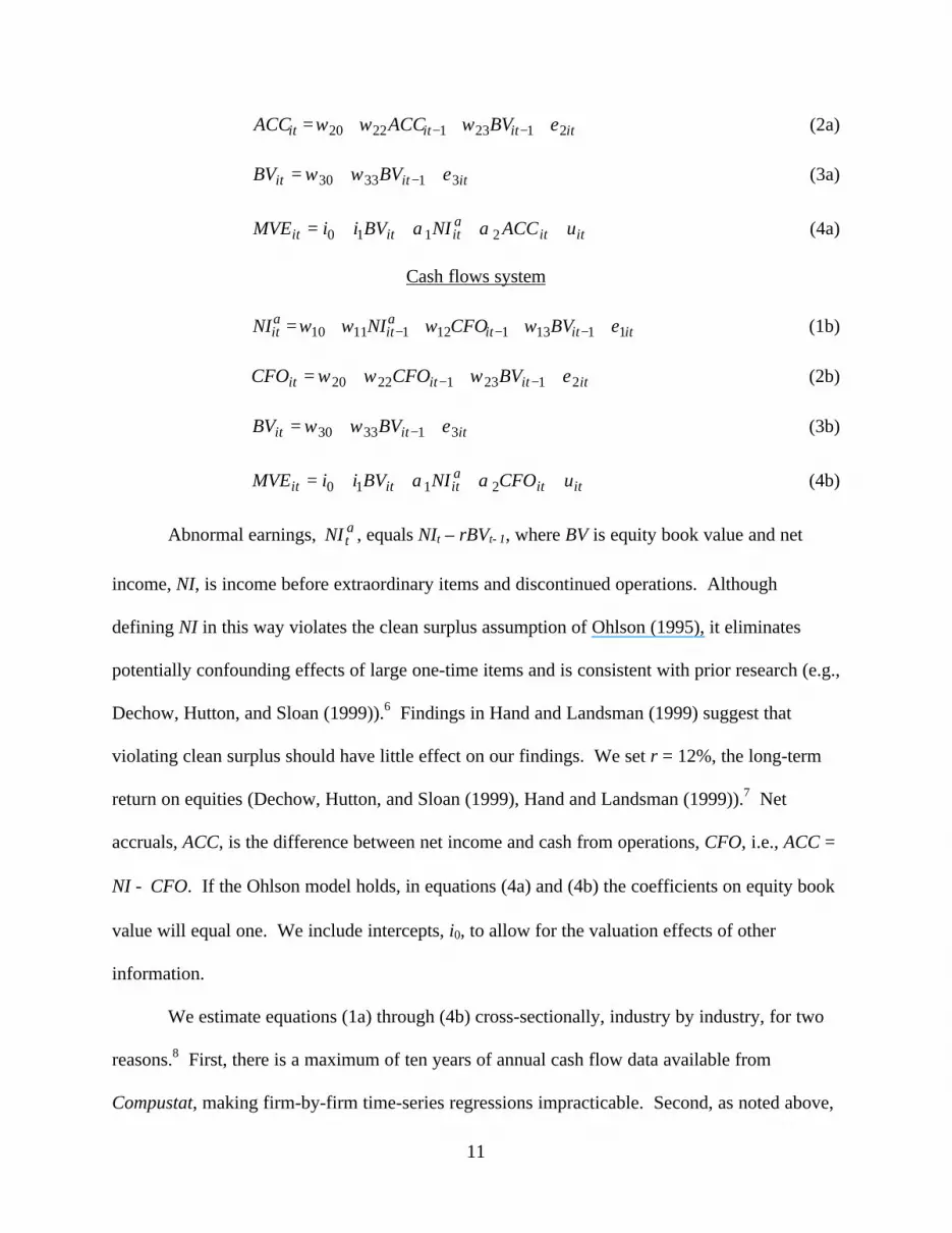
Abnormal earnings, atNI , equals NIt – rBVt−1, where BV is equity book value and net

income, NI, is income before extraordinary items and discontinued operations. Although

defining NI in this way violates the clean surplus assumption of Ohlson (1995), it eliminates

potentially confounding effects of large one-time items and is consistent with prior research (e.g.,

Dechow, Hutton, and Sloan (1999)).6 Findings in Hand and Landsman (1999) suggest that

violating clean surplus should have little effect on our findings. We set r = 12%, the long-term

return on equities (Dechow, Hutton, and Sloan (1999), Hand and Landsman (1999)).7 Net

accruals, ACC, is the difference between net income and cash from operations, CFO, i.e., ACC =

NI − CFO. If the Ohlson model holds, in equations (4a) and (4b) the coefficients on equity book

value will equal one. We include intercepts, i0, to allow for the valuation effects of other

information.

We estimate equations (1a) through (4b) cross-sectionally, industry by industry, for two

reasons.8 First, there is a maximum of ten years of annual cash flow data available from

Compustat, making firm-by-firm time-series regressions impracticable. Second, as noted above,

12

separate industry estimation permits the coefficients to reflect systematic variation in economic

and accounting environments across industries; we view industry membership as a proxy for

these factors. We use the same industry classifications as in Barth, Beaver, and Landsman

(1998).9 All equations are estimated using unscaled data (Barth and Kallapur (1996)).

Because by definition net income equals accruals plus cash flows, one would expect the

findings relating to accruals in equations (1a) and (4a) to be “mirror images” of the findings

relating to cash flows in equations (1b) and (4b). For example, if ω12 is significantly negative in

equation (1a), one would expect ω12 to be significantly positive in equation (1b). Equations (1a)

and (1b) are not econometrically equivalent, however, because each equation contains abnormal

earnings, not net income.10 This also is the case for equations (4a) and (4b). Thus, we report

findings for both the accruals and cash flows systems.

2. Sample Selection and Descriptive Statistics

We obtain data for 1987−1996 from the Compustat Primary, Secondary, and Tertiary,

Full Coverage, and Research Annual Industrial Files. Our sample period begins in 1987

because prior to that date cash flow from operations disclosed under Statement of Financial

Accounting Standards No. 95 (FASB (1987)) is unavailable. To mitigate the effects of outliers,

for each variable, by year and within each industry, we treat as missing observations that are in

the extreme top and bottom one percentile (Kothari and Zimmerman (1995), Collins, Maydew

and Weiss (1997), Fama and French (1998)). We also restrict the sample to firms with full data

to estimate the system of equations and total assets in excess of $10 million to avoid the

influence of small firms. All variables are measured as of fiscal year end, including equity

market value, and are expressed in millions of dollars.

13

Table 1 presents descriptive statistics for each of the variables used in the estimating

equations. Panel A reports distributional statistics, panel B contains Pearson and Spearman

correlations, and panel C describes the industry composition of the sample. Panel A reveals that,

on average, the market value of equity exceeds the book value of equity, indicating that equity

book value alone is insufficient to explain equity market value. Panel A also reveals that, on

average, accruals are negative and cash flows are positive. This is consistent with prior research

(Sloan (1996), Barth, Cram, and Nelson (1998)) and with depreciation expense being included in

accruals but capital expenditures being included in investing cash flows. Panel A also reveals

that mean abnormal earnings is negative, which could be attributable to the cost of capital being

less than 12%.11 Panel B reveals that most of the variables are highly correlated with each other.

Panel C reports the industry breakdown of our sample. Industries with the largest concentrations

of firm-year observations are Durable Manufacturers, 27.3%, and Retail firms, 13.3%.

3. Results

3.1. Abnormal Earnings Equations

Table 2, panels A and B, present regression summary statistics corresponding to the

abnormal earnings equations (1a) and (1b) for each of the fourteen industries. Mean parameter

estimates, t-statistics, and adjusted R2 values across industries are summarized at the bottom of

each panel of table 2 and all subsequent tables in which industry results are presented.

Regarding our first research question, panel A reveals that, as predicted, accruals are

incrementally informative regarding future abnormal earnings for each of the fourteen industries.

Moreover, consistent with predictions based on Sloan (1996), ω12 is significantly negative in all

industries, suggesting that the lower is the proportion of current earnings attributable to accruals,

the higher is future abnormal earnings. Panel A also reveals that ω12 varies substantially across

14

industries. The coefficient estimates (t-statistics) range from −0.75 to −0.02 (−22.51 to −1.67).

The industries with the most extreme coefficients are Pharmaceuticals and Financial institutions.

Because of the link between ω12 in the abnormal earnings equation and α2 in the valuation

equation, these two industries also stand out as exceptions in the valuation equation findings

reported below. In addition, we reject forecasting irrelevance of accruals in each industry, i.e.,

we reject the null hypothesis that ω11 + ω12 = 0.

Consistent with prior research (Dechow, Hutton, and Sloan (1999), Hand and Landsman

(1999)), the coefficient on lagged abnormal earnings, ω11, is positive and significant for all

industries. Although the mean of 0.62 is similar to that reported in prior research, the

coefficients range from 0.27 to 0.94, indicating substantial cross-industry variation in the

persistence of abnormal earnings. Finally, ω13 is always significantly negative, which is

inconsistent with conservatism, but consistent with the cost of capital being less than 12%. In

addition, the cross-industry variation in ω13 suggests that there is inter-industry variation in the

cost of capital and/or the level of conservatism.

The findings relating to cash flows in table 2, panel B, reveal inferences consistent with

those in panel A for accruals. In particular, panel B reveals that, as predicted, cash flows are

significantly incrementally informative regarding future abnormal earnings for all fourteen

industries. The findings also reveal that the sign of ω12 for cash flows is opposite that for

accruals, as expected, i.e., the findings relating to accruals and cash flows in the abnormal

earnings equations are “mirror images” of each other. As with accruals, the ω12 estimates (t-

statistics) vary across industries from 0.02 to 0.66 (2.13 to 23.87), and the industries with the

most extreme coefficients are Pharmaceuticals and Financial institutions. Also, consistent with

the accruals findings, ω12 is significantly positive for all industries, suggesting that the higher is

15

the proportion of current earnings attributable to cash flows, the higher is future abnormal

earnings. Finally, as predicted, we reject forecasting irrelevance for cash flows in each industry,

i.e., we reject the null hypothesis that ω11 + ω12 = 0.

Panel B also reveals that the mean estimated persistence of abnormal earnings, ω11, is

0.37, which is lower than the mean relating to the accruals equation. As with the accruals

equation, there is substantial cross-industry variation in estimates of ω11, 0.16 to 0.76. The

coefficient on lagged equity book value, ω13, is significantly negative in all industries, with

cross-industry variation again suggesting that there is inter-industry variation in the cost of

capital and the level of conservatism.

3.2. Accruals and Cash Flows Autogression Results

Table 3 presents regression summary statistics corresponding to the earnings component

autoregression equations (2a) and (2b). The accruals autoregressions reveal that ω22 is less than

1.00 in all industries, ranging from 0.19 for Utilities to 0.92 for Transportation firms, indicating

stationary autoregressive processes for accruals in all industries. The cash flows autoregressions

indicate that ω22 ranges from 0.31 for Utilities to 1.03 for firms in the Food industry. For all but

two industries, Food and Transportation, ω22 is less than 1.00, indicating, as with accruals, that

the cash flows autoregressive process generally is stationary.12 Comparison of the autoregressive

parameter estimates across industries shows that accruals are less persistent than cash flows for

all but two industries, Mining + construction and Textiles + printing/publishing. The coefficient

on lagged equity book value, ω23, is significantly negative (positive) for accruals (cash flows) in

all industries.

16

3.3. Valuation Equations

Table 4, panels A and B, present regression summary statistics corresponding to the

valuation equations (4a) and (4b). Regarding our second research question, panel A reveals that,

as predicted, α2, the coefficient on accruals, is significantly different from zero in all industries.

This indicates that the accrual component of earnings is incrementally valuation relevant, i.e., the

coefficient on accruals differs from that on abnormal earnings. In addition, α2 is negative for all

industries except Pharmaceuticals and Financial institutions, the two industries with extreme

values for ω12 in table 2, and ranges from –8.34 to 10.89. Also as predicted, we reject the null

hypothesis that α1 + α2 = 0 for every industry, indicating that accruals are valuation relevant,

i.e., their total coefficient in each industry differs from zero.

Recall from equation (5) that the Ohlson model indicates the sign of α2 depends on the

sign of ω12. However, all coefficients in tables 2 through 4 are estimated without imposing the

coefficient restrictions implied by the Ohlson model. Thus, agreement of the signs of ω12 and α2

is initial evidence consistent with predictions relating to our third research question, regarding

whether the valuation multiples on accruals and cash flows vary as predicted by the Ohlson

model. In table 5, below, we provide additional evidence on this question by comparing the α2

estimates in table 4 to those estimated after imposing the coefficient restrictions in equation (5).

Comparing the signs of ω12 in table 2, panel A, and the signs of α2 in table 4, panel A, indicates

they are consistent for all but the two extreme industries in table 2, Pharmaceuticals and

Financial institutions, both of which have positive α2 estimates.

Table 4, panel A, also reveals substantial cross-industry variation in the valuation

coefficients on equity book value and abnormal earnings.13 Although it is significantly positive

17

for all industries, the coefficient on equity book value ranges from 0.99 to 2.91. We reject the

null hypothesis that the coefficient on equity book value equals one in all but one industry,

Extractive industries. These findings suggest that the extent of accounting conservatism varies

across industries. Similarly, the coefficient on abnormal earnings is significantly positive in all

industries and ranges from 4.89 to 21.67.

Turning to the valuation equations for cash flows, the findings in table 4, panel B, also

reveal that, as predicted, α2 is significantly different from zero in all industries. This indicates

that the cash flow component of earnings is incrementally valuation relevant, i.e., the coefficient

on cash flows differs from that on abnormal earnings. In addition, α2 is positive for all

industries, except Pharmaceuticals and Financial institutions, and ranges from –11.25 to 8.05.

As with accruals, we reject the null hypothesis that α1 + α2 = 0 for every industry, indicating that

cash flows are valuation relevant, i.e., their total coefficient differs from zero. As with ω12 in the

abnormal earnings equation, the reversal of signs of α2 between accruals and cash flows in the

valuation equations is consistent with accruals and cash flows being mirror images of each other.

As with accruals, comparing the signs of ω12 in table 2, panel B, and the signs of α2 in table 4,

panel B, indicate they are consistent for all but the same two industries, Pharmaceuticals and

Financial institutions.

Panel B also reveals substantial cross-industry variation in the valuation coefficients on

equity book value and abnormal earnings. The coefficient on equity book value ranges from

0.40 to 3.99, and we reject that it equals one in all industries. As in panel A, the coefficient on

abnormal earnings is significantly positive in all industries and ranges from 1.30 to 33.60.

18

3.4. Estimation of Restricted System of Equations

We now turn to findings relating to our third research question. To test directly

predictions of the Ohlson model, we estimate the accruals system, equations (1a) through (4a),

and the cash flows system, equations (1b) through (4b), but imposing the constraint specified in

equation (5).

Table 5 presents a comparison of the constrained α2 estimates and the unconstrained α2

estimates reported in table 4. As an additional test, table 5 also presents estimates of α2

calculated using the unconstrained estimates of ω11, ω12, and ω22, which we refer to as calculated

α2. Panel A presents the unconstrained, constrained, and calculated α2 estimates, and p-values

from the Wald χ2 statistic corresponding to a test of whether the restriction relating to the

constrained α2 estimate is binding. Panel B presents Pearson and Spearman correlations among

the unconstrained, constrained, and calculated α2 estimates. Note there is no constrained α2

estimate for Pharmaceuticals firms, one of the two extreme industries; convergence failed to

occur during system estimation.

The findings in panel A indicate that the constrained and unconstrained α2 estimates

differ for both accruals and cash flows, and the Wald test indicates that the coefficient constraint

in equation (5) is binding for all but Durable manufacturers in both the accruals and cash flows

systems. However, for both accruals and cash flows, the correlations in panel B indicate that

imposing the constraint results in α2 estimates that are highly positively correlated with

unconstrained α2 estimates. For accruals, the Pearson and Spearman correlations are 0.92 and

0.77; for cash flows, the correlations are 0.91 and 0.94. However, for both accruals and cash

19

flows, panel B indicates no consistent positive correlation between the calculated α2 estimates

and either the constrained or unconstrained α2 estimates.14

Finding that the constrained and unconstrained α2 estimates correlate highly but no

consistent positive association between the calculated and the constrained and unconstrained

estimates suggests the possibility that, for the constrained accruals and cash flows systems, the

valuation regressions “dominate” the autoregressive equations in minimizing the system

weighted sum of squared residuals. If this is the case, then the constrained and unconstrained ωs

should not be significantly correlated. However, table 5, panel C, which presents Pearson and

Spearman correlations between constrained and unconstrained estimates for ω11, ω12, and ω22,

indicates high correlation between the estimates for both accruals and cash flows. The Pearson

(Spearman) correlations range from 0.81 to 0.99 (0.66 to 0.99). Hence, the lack of consistent

positive correlation between the calculated α2 and the unconstrained and constrained α2

estimates appears to be the result of other factors.

One possible explanation is that, although the Ohlson model provides a parsimonious

description of the mapping from accounting data into equity value, the model may not be entirely

descriptively valid. For example, our empirical estimations exclude consideration of “other

information,” because, if the model holds, it has no bearing on parameters relating to accounting

data, abnormal earnings, equity book value, and the accrual and cash flow earnings components.

However, evidence presented in tables 2, 4, and 5 indicates the model performs particularly

poorly for Pharmaceuticals and Financial institutions, two industries for which other information

could be significant in determining future abnormal earnings and current equity value. Thus, if

other information and accounting data are not unrelated, i.e., the model does not literally hold,

20

parameter estimates for accounting amounts could be affected by omitting consideration of other

information in the estimating equations.

A second possible explanation is that even if the model is descriptively valid, it relates to

a particular firm as of a particular date. Even though we permit coefficients to vary across

industries, we constrain them to be cross-sectional constants within industries. In addition,

although we allow for year-specific intercepts, all other coefficients are intertemporal constants.

Relatedly, Collins, Pincus, and Xie (1998) and Hand and Landsman (1999) find that Ohlson

model valuation estimates differ for positive and negative earnings firms. We examine below

whether pooling positive and negative earnings firms affects our inferences. Finally, it is

possible that prices do not reflect fully differences in valuation implications for accruals and cash

flows (Sloan (1996), Barth and Hutton (1999), Frankel and Lee (1999), Dechow, Hutton and

Sloan (1999), Lee, Myers, and Swaminathan (1999)).15

Nonetheless, taken together, the findings in tables 2 through 5 provide support for the

prediction that accruals and cash flows are incrementally informative in predicting future

abnormal earnings and in explaining current equity market values. In addition, accruals and cash

flows have forecasting and valuation relevancy in all industries. Moreover, correspondence in

sign between α2 and ω12 for all but two industries for both accruals and cash flows confirms the

link between forecasting relevancy and valuation relevancy.16

3.5. Positive Earnings Sample

As noted above, prior research finds that Ohlson model valuation estimates differ for

positive and negative earnings firms. This is predictable from the Ohlson model given that

negative earnings is less persistent than positive earnings (Hayn (1995), Collins, Maydew and

Weiss (1997), Collins, Pincus, and Xie (1999)). The findings presented in tables 2 through 4 are

21

based on all firm-years without regard to the sign of earnings. Thus, we reestimate the

unconstrained and constrained accruals and cash flows systems, limiting the samples to positive

earnings firm-years. Table 6, panels A and B, present the findings for accruals and cash flows.

Panel C presents the correlations among the unconstrained, constrained, and calculated α2

estimates.

Although the positive earnings sample comprises only approximately 60% of the full

sample, the findings in table 6 largely support those presented for the full sample. As expected,

the persistence of abnormal earnings as measured by ω11 is higher for the positive earnings

subsample, with means of 0.68 and 0.41 for accruals and cash flows versus 0.62 and 0.37 for the

full sample. With the exception of one industry, Mining + construction, the abnormal earnings

forecasting coefficients on accruals and cash flows, ω12, are comparable to those based on the

full sample. Also as expected, estimates of the earnings components’ persistence parameters,

ω22, are higher than those based on the full sample.

Turning to the valuation equations, the signs of α2 generally are the same as those based

on the full sample. The p-values in panels A and B indicate that the equation (5) constraint is

binding in fewer industries for positive earnings firms than is the case for the full sample. Panel

C reveals that the correlations between the constrained and unconstrained estimates of α2 are

similar to those based on the full sample reported in table 5. However, the correlations between

the calculated α2 and the constrained and unconstrained α2 estimates generally are higher than

those reported in table 5. Taken together, the findings in table 6 suggest that inferences relating

to the full sample are largely unaffected by constraining coefficients to be the same for negative

and positive earnings firms.

22

4. Summary and Concluding Remarks

This study provides insights into the characteristics of the accrual and cash flow

components of earnings that affect their relation with firm value. We base our analysis on the

valuation framework in Ohlson (1999), in which the value relevance of an earnings component

depends on its ability to predict future abnormal earnings incremental to abnormal earnings and

the persistence of the component. Using a sample of Compustat firms with available annual data

between 1987-1996, we implement the Ohlson (1999) model by estimating two sets of four

jointly estimated equations, one set each for accruals and cash flows. Based on these estimating

equations, we address three research questions relating to the accrual and cash flow components

of earnings.

Relating to our first research question, as predicted, we find that for all industries,

accruals and cash flows each have significant explanatory power in forecasting future abnormal

earnings incremental to abnormal earnings. That is, the two components do not have the same

ability to predict future abnormal earnings. In particular, the coefficients on accruals and cash

flows are negative and positive, indicating abnormal earnings is less persistent when accruals

comprise a larger proportion of current earnings. We also find that accruals and cash flows have

forecasting relevance in that each has a significant relation with future abnormal earnings. There

is considerable cross-industry variation in the magnitude of the coefficients on the components in

the abnormal earnings forecasting equation.

Relating to our second research question, we find that for all industries, as predicted,

accruals and cash flows each have significant incremental explanatory power in the relations

between market value of equity and equity book value, abnormal earnings, and each earnings

component. That is, knowing the accrual and cash flow components of earnings helps explain

23

market value of equity, incremental to knowing equity book value and abnormal earnings. In

particular, as predicted based on the findings of the abnormal earnings forecasting analysis and

the Ohlson model, the coefficients are predominantly negative for accruals and positive for cash

flows. We also find, as predicted, that both components have value relevance in that their

estimated total valuation coefficients differ from zero, indicating they each have a significant

relation with equity market value. As with abnormal earnings prediction equations, there is

considerable cross-industry variation in the valuation coefficients on the earnings components.

Relating to our third research question, we find evidence that the valuation coefficients

on accruals and cash flows vary as predicted by the Ohlson model based on the persistence of the

components and their ability to predict future abnormal earnings. In particular, as noted above,

there is considerable agreement between the signs of the valuation and abnormal earnings

equations coefficients on accruals and cash flows. However, we find that the correlations

between the estimated component valuation coefficients and those calculated from the abnormal

earnings and component autoregressive equations and implied by the Ohlson model are not

consistently positive. We also find that the constraint on the accruals and cash flows valuation

coefficients implied by the Ohlson model is binding for most industries. Yet, the correlations

across industries between the constrained and unconstrained valuation coefficient estimates are

high.

Prior accruals and cash flows research investigating potential differences in value

relevance for the two components focuses primarily on the persistence of the components in

predicting future earnings and cash flows. Taken together, our findings suggest that, consistent

with the accounting-based valuation model of Ohlson (1999), the interaction between two key

characteristics of the components, their ability to aid in forecasting future abnormal earnings and

24

the persistence of the components themselves, results in different valuation implications of the

accrual and cash flow components of earnings.

25

Acknowledgements

We thank Ed Maydew, James Myers, Jim Ohlson, Stephen Penman (editor), an anonymous

reviewer, and workshop participants at UCLA, University of Colorado, University of Michigan

1999 Spring Training, University of North Carolina, University of Oregon, University of

Washington, and the 1999 Review of Accounting Studies Conference, especially discussant

Richard Sloan, for helpful comments. We appreciate funding from the Financial Research

Initiative, Graduate School of Business, Stanford University, the Center for Finance and

Accounting Research at UNC-Chapel Hill, and NationsBank Research Fellowships.

26

References

Ali, A. (1994). The Incremental Information Content of Earnings, Working Capital from

Operations, and Cash Flow.” Journal of Accounting Research 32, 61–74.

Barth, M.E., W.H. Beaver and W.R. Landsman. (1992). “The Market Valuation Implications of

Net Periodic Pension Cost.” Journal of Accounting and Economics 15, 27–62.

Barth, M.E., W.H. Beaver and W.R. Landsman (1998). “Relative Valuation Roles of Equity

Book Value and Net Income as a Function of Financial Health.” Journal of Accounting and

Economics 25, 1–34.

Barth, M.E., W.H. Beaver, and M.A. Wolfson. (1990). “Components of Bank Earnings and the

Structure of Bank Share Prices.” Financial Analysts Journal, May/June, 53-60.

Barth, M.E., D.P. Cram, and K.K. Nelson. (1998). “Accruals and the Prediction of Future Cash

Flow.” working paper, Stanford University.

Barth, M.E. and A.P. Hutton. (1999). “Information Intermediaries and the Pricing of Accruals.”

working paper, Stanford University.

Barth, M.E, and S. Kallapur (1996). “Effects of Cross-Sectional Scale Differences on Regression

Results in Empirical Accounting Research.” Contemporary Accounting Research 13, 527-

567.

Bernard, V.L., and T.L. Stober. (1989). “The Nature and Amount of Information in Cash Flows

and Accruals.” The Accounting Review 64, 624–652.

Bowen, M., D. Burgstahler, and L.A. Daley. (1987). “The Incremental Information Content of

Accrual Versus Cash Flows.” The Accounting Review 62, 723–747.

Collins, D.W., Maydew, E.L., and I.S. Weiss. (1997). “Changes in the Value-Relevance of

Earnings & Equity Book Values Over The Past Forty Years.” Journal of Accounting and

27

Economics 24, 39-67.

Collins, D.W., M. Pincus, and H. Xie. (1999). “Equity Valuation and Negative Earnings: The Role

of Negative Earnings.” Accounting Review 74, 29-61.

Dechow, P.M. (1994). “Accounting Earnings and Cash Flows as Measures of Firm Performance:

the Role Accounting Accruals.” Journal of Accounting and Economic 18, 3-42.

Dechow, P.M., Hutton, A.P., and R.G. Sloan. (1999). “An Empirical Assessment of the Residual

Income Valuation Model.” Journal of Accounting and Economics 26, 1-34.

Fama, E.F., and K.R. French. (1998). “Taxes, Financing Decisions, and Firm Value.” Journal of

Finance 53, June.

Feltham, G.A., and J.A. Ohlson. (1995). “Valuation and Clean Surplus Accounting for Operating

and Financial Activities.” Contemporary Accounting Research 11, 689-732.

Feltham, G.A., and J.A. Ohlson. (1996). “Uncertainty Resolution and the Theory of Depreciation

Measurement.” Journal of Accounting Research 34, 209-234.

Financial Accounting Standards Board. (1987). Statement of Financial Accounting Standards

No. 95: Statement of Cash Flows (FASB, Stamford, CT).

Frankel, R., and C. Lee. (1998). “Accounting Valuation, Market Expectation, and the Book-to-

Market Effect.” Journal of Accounting and Economics 25, 283-319.

Hand, J.R.M., and W. Landsman. (1999). “The Pricing of Dividends and Equity Valuation.”

working paper, University of North Carolina.

Hayn, C. (1995). “The Information Content of Losses.” Journal of Accounting and Economics

20, 125-133.

Kormendi, R., and R. Lipe. (1987). “Earnings Innovations, Earnings Persistence and Stock

Returns.” Journal of Business July, 323-345.

28

Kothari, S.P., and J. Zimmerman. (1995). “Price and Return Models.” Journal of Accounting and

Economics 20, 155-192.

Lee, C., J. Myers, and B. Swaminathan. (1999). “What is the Intrinsic Value of the Dow?”

Journal of Finance, Forthcoming.

Lipe, R.C. (1986). “The Information Contained in the Components of Earnings.” Journal Of

Accounting Research 24, 37–64.

Myers, J. (1999). “Implementing Residual Income Valuation with Linear Information

Dynamics.” The Accounting Review 74, 1-28.

Ohlson, J.A. (1995). “Earnings, Equity Book Values, and Dividends in Equity Valuation.”

Contemporary Accounting Research, 66-687.

Ohlson, J.A. (1999). “On Transitory Earnings.” Review of Accounting Studies, This Issue.

Ohlson, J.A., And X. Zhang. (1998). “Accrual Accounting And Equity Valuation.” Journal of

Accounting Research 36, 85-115.

Rayburn, J. (1986). “The Association of Operating Cash Flow and Accruals with Security

Returns.” Journal Of Accounting Research (Supplement): 112-133.

Sloan, R.G. (1996). “Do Stock Prices Fully Reflect Information in Accruals and Cash Flows

About Future Earnings?” The Accounting Review 71, 289-315.

Wilson, G.P. (1986). “The Relative Information Content of Accruals and Cash Flows: Combined

Evidence at the Earnings Announcement and Annual Report Release Date.” Journal of

Accounting Research 24 (Suppl.): 165-200.

Wilson, G.P. (1987). “The Incremental Information Content of the Accrual and Funds

Components of Earnings After Controlling for Earnings.” The Accounting Review 62: 293-

322.

29

Table 1

Descriptive statistics for the sample of 15,405 Compustat firm year observations, 1987 – 1996.

Panel A: Distributional statistics (in $ millions)

Description Variable Mean Median Std dev Market value of equity MVE 506.18 94.37 1,511.74

Book value of equity BV 231.05 54.74 637.09

Market-to-book ratio MB 2.19 1.58 18.27

Abnormal earnings NIa –0.79 –0.80 57.63

Accruals ACC –33.75 –4.70 128.06

Cash flows CFO 58.54 8.16 199.49

Panel B: Correlations, with Pearson (Spearman) correlations above (below) the diagonal

Variable MVE BV NIa ACC CFO MVE 0.85 0.39 –0.65 0.83

BV 0.88 0.12 –0.78 0.89

NIa 0.30 0.16 0.02 0.30

ACC –0.41 –0.45 0.16 –0.71

CFO 0.71 0.73 0.29 –0.92

30

Table 1 (continued)

Descriptive statistics for the sample of 15,405 Compustat firm year observations, 1987 – 1996.

Panel C: Industry composition

Ιndustry Primary SIC codes # firm- years

% of obs.

1 Mining + construction 1000 − 1999, excluding 1300 – 1399 401 2.62 Food 2000 − 2111 420 2.33 Textiles + printg/pubg 2200 – 2780 1,018 6.64 Chemicals 2800 – 2824, 2840 – 2899 341 2.15 Pharmaceuticals 2830 – 2836 410 2.66 Extractive industries 2900 – 2999, 1300 – 1399 628 4.17 Durable manufacturers 3000 – 3999, excluding 3570 – 3579

and 3670 – 36794,079 27.3

8 Computers 7370 – 7379, 3570 – 3579, 3670 – 3679 911 6.59 Transportation 4000 – 4899 862 4.810 Utilities 4900 – 4999 1,109 6.811 Retail 5000 – 5999 2,027 13.312 Financial institutions 6000 – 6411 1,017 5.313 Insurance + real estate 6500 – 6999 893 6.114 Services 7000 – 8999, excluding 7370 – 7379 1,289 8.9

Total 15,405 100.0

Mean 1,100 7.1 Abnormal earnings NIa is net income before extraordinary items and discontinued operations, NI,minus 0.12 â book value of equity, BV, lagged one year. Accruals, ACC, is NI minus cash flowsfrom operations, CFO, disclosed under SFAS 95. MVE is market value of equity at fiscal yearend.

31

Table 2

Summary statistics from regressions of abnormal earnings on lagged abnormal earnings and accruals or cash flows.Sample of 15,405 Compustat firm year observations, 1987 – 1996.

Panel A: Accruals: itititait

ait BVACCNINI 111311211110 εωωωω ++++= −−−

ω11 ω12 ω13 ω11+ω12=0

Industry coef t-stat coef t-stat coef t-stat p-value Adj.R2 Mining + construction 0.40 9.82 –0.06 –1.67 –0.47 –7.20 < 0.01 0.40

Food 0.86 28.25 –0.45 –11.85 –0.03 –6.41 < 0.01 0.76

Textiles + printg/pubg 0.27 11.82 –0.11 –4.07 –0.05 –11.05 < 0.01 0.28

Chemicals 0.63 15.44 –0.22 –4.38 –0.06 –6.59 < 0.01 0.29

Pharmaceuticals 0.94 28.74 –0.75 –12.20 –0.02 –1.90 < 0.01 0.89

Extractive industries 0.59 16.59 –0.26 –10.68 –0.06 –12.38 < 0.01 0.33

Durable manufacturers 0.55 50.58 –0.24 –22.51 –0.05 –24.72 < 0.01 0.41

Computers 0.38 10.00 –0.10 –2.72 –0.07 –7.99 < 0.01 0.14

Transportation 0.88 37.73 –0.17 –8.82 –0.03 –6.03 < 0.01 0.65

Utilities 0.36 16.18 –0.04 –3.15 –0.01 –4.13 < 0.01 0.15

Retail 0.67 36.22 –0.11 –8.86 –0.01 –4.23 < 0.01 0.43

Financial institutions 0.69 26.11 –0.02 –2.58 –0.01 –5.06 < 0.01 0.36

Insurance + real estate 0.83 39.27 –0.29 –8.94 –0.01 –4.22 < 0.01 0.43

Services 0.69 32.31 –0.10 –7.07 –0.03 –7.49 < 0.01 0.41

Mean 0.62 25.65 −0.25 −7.82 −0.07 −7.81 0.42

32

Table 2 (continued)

Summary statistics from regressions of abnormal earnings on lagged abnormal earnings and accruals or cash flows.Sample of 15,405 Compustat firm year observations, 1987 – 1996.

Panel B: itititait

ait BVCFONINI 111311211110 εωωωω ++++= −−−

ω11 ω12 ω13 ω11+ω12=0

Industry coef t-stat coef t-stat coef t-stat p-value Adj R2 Mining + construction 0.43 10.82 0.10 2.86 –0.06 –7.14 < 0.01 0.42

Food 0.16 3.49 0.52 15.92 –0.09 –10.72 < 0.01 0.76

Textiles + printg/pubg. 0.23 9.54 0.10 3.87 –0.06 –8.85 < 0.01 0.29

Chemicals 0.18 4.12 0.27 5.89 –0.10 –7.28 < 0.01 0.26

Pharmaceuticals 0.26 6.19 0.66 13.67 –0.07 –5.58 < 0.01 0.90

Extractive industries 0.19 4.89 0.26 11.49 –0.09 –12.77 < 0.01 0.32

Durable manufacturers 0.26 20.68 0.25 23.87 –0.07 –28.24 < 0.01 0.40

Computers 0.21 6.65 0.08 2.13 –0.07 –5.90 < 0.01 0.13

Transportation 0.76 34.87 0.16 9.38 –0.05 –7.40 < 0.01 0.66

Utilities 0.25 11.76 0.03 2.50 –0.01 –3.39 < 0.01 0.14

Retail 0.57 31.08 0.12 9.83 –0.02 –7.47 < 0.01 0.43

Financial institutions 0.65 24.48 0.02 2.85 –0.01 –5.03 < 0.01 0.36

Insurance + real estate 0.47 16.81 0.31 8.57 –0.05 –8.09 < 0.01 0.43

Services 0.53 22.62 0.10 7.28 –0.04 –8.09 < 0.01 0.41

Mean 0.37 14.86 0.21 8.58 –0.06 –9.00 0.42 Variable definitions and number of observations by industry are per table 1. Tables 2, 3, and 4 estimates are based on SeeminglyUnrelated Regression estimation of the system of equations.

33

Table 3

Summary statistics from first-order autoregressions of accruals and cash flows.Sample of 15,405 Compustat firm year observations from 1987 to 1996.

itititit BVACCACC 212312220 εωωω +++= −− itititit BVCFOCFO 212312220 εωωω +++= −−

ω22 ω23 ω22 ω23

Industry coef t-stat coef t-stat Adj.R2 coef t-stat coef t-stat Adj.R2 Mining + construction 0.47 9.19 −0.04 –3.57 0.40 0.38 7.00 0.07 6.18 0.39

Food 0.58 13.03 −0.06 –10.82 0.74 1.03 44.91 0.02 2.52 0.97

Textiles + printg/pubg 0.42 11.02 −0.09 –14.89 0.68 0.41 11.94 0.13 14.95 0.76

Chemicals 0.23 5.24 −0.11 –14.81 0.84 0.69 16.98 0.06 4.55 0.89

Pharmaceuticals 0.28 3.87 −0.04 –5.00 0.51 0.99 22.03 0.04 2.63 0.96

Extractive industries 0.50 15.40 −0.11 –16.33 0.89 0.79 28.14 0.07 7.79 0.95

Durable manufacturers 0.42 25.56 −0.08 –31.94 0.57 0.75 53.53 0.07 19.42 0.82

Computers 0.45 10.77 −0.06 –7.86 0.52 0.64 14.85 0.03 1.86 0.59

Transportation 0.92 43.98 −0.03 –5.44 0.90 1.02 48.58 0.02 2.75 0.94

Utilities 0.19 7.20 −0.14 –26.85 0.82 0.31 11.04 0.20 24.03 0.93

Retail 0.46 22.33 −0.04 –13.58 0.40 0.58 27.82 0.10 18.40 0.77

Financial institutions 0.48 21.42 −0.09 –13.47 0.53 0.52 22.80 0.15 17.61 0.72

Insurance + real estate 0.53 16.35 −0.03 –8.26 0.39 0.88 34.08 0.05 11.15 0.89

Services 0.79 35.11 −0.06 –9.85 0.63 0.89 44.29 0.06 9.03 0.79

Mean 0.48 17.18 –0.07 –13.05 0.63 0.71 27.71 0.08 10.21 0.81 Variable definitions and number of observations by industry are per table 1. Tables 2, 3, and 4 estimates are based on SeeminglyUnrelated Regression estimation of the system of equations.

34

Table 4

Summary statistics from regressions of market value of equity on book value of equity, abnormal earnings, and accruals or cash flows.Sample of 15,405 Compustat firm year observations, 1987 – 1996.

Panel A: Accruals: ititaititit uACCNIBViiMVE ++++= 2110 αα

i1 α1 α2 p-values

Industry coef t-stat coef t-stat coef t-stat i1 = 1 α1+α2=0 Adj.R2 Mining + construction 1.83 23.11 6.14 9.85 –4.89 –11.37 < 0.01 0.01 0.63

Food 2.10 26.46 7.64 14.47 –1.83 –3.10 < 0.01 < 0.01 0.87

Textiles + printg/pubg 1.67 39.48 4.89 18.27 –0.65 –2.65 < 0.01 < 0.01 0.79

Chemicals 1.24 12.85 7.05 16.06 –4.97 –8.26 0.01 < 0.01 0.83

Pharmaceuticals 2.91 16.60 21.67 23.30 10.89 7.21 < 0.01 < 0.01 0.92

Extractive industries 0.99 26.01 5.74 28.61 –4.52 –24.61 0.79 < 0.01 0.96

Durable manufacturers 2.09 90.73 6.66 40.86 –0.52 –3.72 < 0.01 < 0.01 0.80

Computers 2.67 32.48 12.39 29.73 –6.57 –12.60 < 0.01 < 0.01 0.78

Transportation 2.03 26.36 5.30 15.04 –1.57 –5.72 < 0.01 < 0.01 0.76

Utilities 1.39 57.92 5.37 20.84 –0.44 –3.30 < 0.01 < 0.01 0.94

Retail 2.03 59.18 13.05 39.58 –1.86 –8.15 < 0.01 < 0.01 0.81

Financial institutions 1.59 60.69 9.62 28.43 0.32 3.08 < 0.01 < 0.01 0.84

Insurance + real estate 1.43 40.10 10.19 24.21 –8.34 –18.41 < 0.01 < 0.01 0.82

Services 2.25 35.77 9.55 22.35 –2.18 –8.93 < 0.01 < 0.01 0.68

Mean 1.87 39.12 8.95 23.69 –1.94 –7.18 0.82

35

Table 4 (continued)

Summary statistics from regressions of market value of equity on book value of equity, abnormal earnings, and accruals or cash flows.Sample of 15,405 Compustat firm year observations, 1987 – 1996.

Panel B: ititaititit uCFONIBViiMVE ++++= 2110 αα

i1 α1 α2 p-values

Industry coef t-stat coef t-stat coef t-stat i1 = 1 α1+α2=0 Adj.R2 Mining + construction 1.28 13.10 1.43 2.84 4.66 10.58 < 0.01 < 0.01 0.62

Food 1.70 14.04 3.95 4.73 2.96 5.53 < 0.01 < 0.01 0.87

Textiles + printg/pubg 1.49 23.08 3.96 12.90 1.10 4.56 < 0.01 < 0.01 0.79

Chemicals 0.55 3.69 2.11 4.03 5.26 9.72 < 0.01 < 0.01 0.84

Pharmaceuticals 3.99 14.18 33.60 21.28 −11.25 –7.87 < 0.01 < 0.01 0.92

Extractive industries 0.40 7.18 1.30 5.69 4.73 26.90 < 0.01 < 0.01 0.96

Durable manufacturers 2.01 57.84 6.22 36.10 0.62 4.53 < 0.01 < 0.01 0.80

Computers 1.86 15.13 6.14 11.27 7.06 13.74 < 0.01 < 0.01 0.78

Transportation 1.81 18.13 3.63 8.96 1.72 6.44 < 0.01 < 0.01 0.77

Utilities 1.33 34.88 4.99 19.47 0.47 3.55 < 0.01 < 0.01 0.94

Retail 1.90 37.78 11.43 35.38 1.50 6.78 < 0.01 < 0.01 0.81

Financial institutions 1.64 49.48 9.90 29.65 −0.36 −3.55 < 0.01 < 0.01 0.84

Insurance + real estate 0.65 9.72 2.96 8.34 8.05 18.26 < 0.01 < 0.01 0.81

Services 2.03 27.18 7.63 17.74 2.17 9.24 < 0.01 < 0.01 0.68

Mean 1.62 23.24 7.09 15.60 2.05 7.74 0.82

Variable definitions and number of observations by industry are per table 1. Tables 2, 3, and 4 estimates are based on SeeminglyUnrelated Regression estimation of the system of equations.

36

Table 5

Comparisons between unconstrained estimates of valuation coefficients on accruals and cash flows, estimates constrained by model ofassumed information dynamics, and estimates calculated from unconstrained parameters.

Sample of 15,405 Compustat firm year observations, 1987 – 1996.

Panel A: Comparison of unconstrained, constrained, and calculated α2 estimates.

Accruals Cash Flows

Industry Unconst. Constr. Calcd. p-value Unconst. Constr. Calcd. p-value Mining + construction –4.89 –0.85 –0.14 < 0.01 4.66 0.99 0.22 < 0.01

Food –1.83 –3.12 –3.65 0.02 2.96 3.88 6.94 0.06

Textiles + printg/pubg –0.65 –0.23 –0.21 0.08 1.10 0.21 0.17 < 0.01

Chemicals –4.97 –2.85 –0.56 < 0.01 5.26 3.91 0.74 < 0.01

Pharmaceuticals 10.89 13.65 –5.78 < 0.01 –11.25 n.a. 6.59 < 0.01

Extractive industries –4.52 –4.22 –0.88 < 0.01 4.73 4.35 0.93 < 0.01

Durable manufacturers –0.52 –0.67 –0.69 0.25 0.62 0.82 0.87 0.10

Computers –6.57 –1.04 –0.23 < 0.01 7.06 6.46 0.20 < 0.01

Transportation –1.57 –2.17 –4.05 < 0.01 1.72 2.16 4.97 0.02

Utilities –0.44 –0.08 –0.06 < 0.01 0.47 0.07 0.05 < 0.01

Retail –1.86 –0.56 –0.43 < 0.01 1.50 0.55 0.45 < 0.01

Financial institutions 0.32 –0.03 –0.07 < 0.01 –0.36 0.03 0.07 < 0.01

Insurance + real estate –8.34 –7.43 –1.91 < 0.01 8.05 7.43 2.31 < 0.01

Services –2.18 –1.19 –0.81 < 0.01 2.17 1.46 0.83 < 0.01

Mean –1.94 –0.77 –1.39 2.05 2.31 1.81

37

Table 5 (continued)

Comparisons between unconstrained estimates of valuation coefficients on accruals and cash flows, estimates constrained by model ofassumed information dynamics, and estimates calculated from unconstrained parameters.

Sample of 15,405 Compustat firm year observations, 1987 – 1996.

Panel B: Correlations across industries between unconstrained, constrained, and calculated α2 estimates. Pearson (Spearman)correlations are above (below) the diagonal.

Accruals

Unconstr. Constr. Calcd.Unconstr. – 0.92 –0.57

– (< 0.01) (0.03)

Constr. 0.77 – –0.48(< 0.01) – (0.08)

Calcd. 0.05 0.46 –(0.85) (0.10) –

Cash Flows

Unconstr. Constr. Calcd.Unconstr. – 0.91 –0.44

– (< 0.01) (0.12)

Constr. 0.94 – 0.30(< 0.01) – (0.32)

Calcd. 0.19 0.63 –(0.51) (0.02) –

38

Table 5 (continued)Comparisons between unconstrained estimates of valuation coefficients on cash from operations and net accruals, estimates

constrained by assumed model of information dynamics, and estimates calculated from unconstrained parameters.Sample of 15,405 Compustat firm year observations, 1987 – 1996.

Panel C: Correlations across industries between unconstrained and constrained estimates of ω11, ω12, and ω22 (p-values).

Accruals Cash Flows Pearson Spearman Pearson Spearman

ω11 0.82 0.79 0.99 0.97(< 0.01) (< 0.01) (< 0.01) (< 0.01)

ω12 0.91 0.82 0.81 0.81(< 0.01) (< 0.01) (< 0.01) (< 0.01)

ω22 1.00 0.99 0.83 0.66(< 0.01) (< 0.01) (< 0.01) 0.01

Variable definitions and number of observations by industry are per table 1. Parameter estimates are based on Seemingly Unrelated

Regression estimation of the following systems of equations: [1] itititait

ait BVACCNINI 111311211110 εωωωω ++++= −−− ,

itititit BVACCACC 212312220 εωωω +++= −− , ititit BVBV 313330 εωω ++= − , and ititaititit uACCNIBViiMVE ++++= 2110 αα for

accruals, and [2] itititait

ait BVCFONINI 111311211110 εωωωω ++++= −−− , itititit BVCFOCFO 212312220 εωωω +++= −− ,

ititit BVBV 313330 εωω ++= − , and ititaititit uCFONIBViiMVE ++++= 2110 αα for cash flows. The autoregressive equation for BV

is estimated but not tabulated. Constrained α2 is the estimate of α2 estimated from the system of equations in which α2 is constrainedto equal ω12 / [(1.12 – ω11)(1.12 – ω22), as predicted by the model’s information dynamics. The p-value in panel A refers to a Waldχ2

test of whether the constraint on α2 is binding. Calculated α2 equals ω12 / [(1.12 – ω11)(1.12 – ω22)], where the ωs are estimated inan unconstrained system.

39

Table 6

Summary statistics from system of equations including market value of equity, book value of equity, abnormal earnings, and accrualsand cash flows. Subsample of 9,369 Compustat firms with NI > 0 in any firm-years 1987 – 1996.

Panel A: Accruals system itititait

ait BVACCNINI 111311211110 εωωωω ++++= −−− itititit BVACCACC 212312220 εωωω +++= −−

ititaititit uACCNIBViiMVE ++++= 2110 αα

ω11 ω12 ω22 α2

Industry coef t-stat coef t-stat coef t-stat coef t-stat α2 constr α2 calcd. p-value N Mining + construction 0.40 4.63 0.01 0.21 0.62 7.13 –4.53 –6.51 –4.00 0.03 < 0.01 179

Food 0.88 23.37 –0.43 –8.93 0.64 11.23 –1.49 –2.10 –3.10 –3.93 0.01 309

Textiles + printg/pubg. 0.37 10.66 –0.11 –2.91 0.59 10.38 –0.86 –2.77 –0.37 –0.30 0.09 686

Chemicals 0.67 15.81 0.30 –5.93 0.25 5.31 –4.86 –6.81 –1.98 –0.86 < 0.01 252

Pharmaceuticals 0.93 14.70 –0.73 –5.62 0.32 2.03 13.41 5.94 n.a. –5.35 < 0.01 117

Extractive industries 0.61 11.43 –0.23 –7.04 0.50 10.83 –4.64 –17.74 –4.46 –0.83 < 0.01 318

Durable manufacturers 0.36 20.25 –0.19 –14.71 0.46 18.95 0.72 3.39 –0.40 –0.43 < 0.01 2,306

Computers 0.86 20.68 –0.13 –2.62 0.48 7.67 –3.63 –3.94 –1.43 –0.87 < 0.01 506

Transportation 0.88 25.93 –0.16 –7.23 0.90 31.51 1.41 4.87 0.82 –3.31 < 0.01 480

Utilities 0.40 16.46 –0.03 –2.82 0.18 6.40 –0.09 –0.62 –0.06 –0.06 0.83 956

Retail 0.74 30.27 –0.09 –6.24 0.48 16.45 –1.10 –4.10 –0.49 –0.43 0.02 1,239

Financial institutions 0.75 27.42 –0.02 –3.63 0.48 18.93 0.50 4.54 –0.02 –0.11 < 0.01 816

Insurance + real estate 0.88 29.20 –0.16 –3.20 0.82 14.79 –8.78 –13.18 –7.95 –2.40 < 0.11 511

Services 0.81 23.99 –0.06 –3.65 0.86 28.15 –1.12 –3.54 –0.92 –0.79 0.41 694

Mean 0.68 19.63 –0.19 0.02 0.54 13.55 –1.08 –3.04 –1.87 –1.40 669

40

Table 6 (continued)

Summary statistics from system of equations including market value of equity, book value of equity, abnormal earnings, and accrualsand cash flows. Subsample of 9,369 Compustat firms with NI > 0 in any firm-years 1987 – 1996.

Panel B: Cash Flows system itititait

ait BVCFONINI 111311211110 εωωωω ++++= −−−

itititit BVCFOCFO 212312220 εωωω +++= −− ititaititit uCFONIBViiMVE ++++= 2110 αα

ω11 ω12 ω22 α2

Industry coef t-stat coef t-stat coef t-stat coef t-stat α2 constr α2 calcd. p-value N Mining + construction 0.47 5.31 –0.02 –0.39 0.53 6.86 4.25 5.94 4.54 –0.05 < 0.01 179

Food 0.17 2.93 0.52 13.02 1.04 36.71 2.66 4.10 3.71 7.17 0.11 309

Textiles + printg/pubg. 0.34 9.42 0.09 2.75 0.61 12.70 1.27 4.16 0.40 0.26 < 0.01 686

Chemicals 0.19 4.17 0.35 7.75 0.77 17.33 4.92 7.67 3.61 1.20 < 0.01 252

Pharmaceuticals 0.26 3.24 0.57 5.78 0.91 9.35 –13.02 –6.02 n.a. 3.65 < 0.01 117

Extractive industries 0.16 2.76 0.25 8.04 0.78 19.73 5.00 20.10 4.63 0.84 < 0.01 318

Durable manufacturers 0.21 11.24 0.19 15.12 0.63 27.48 -0.42 –2.02 0.44 0.49 < 0.01 2,306

Computers 0.45 9.39 0.25 5.86 0.76 15.75 2.23 2.56 1.32 1.16 0.25 506

Transportation 0.62 17.28 0.18 8.94 1.02 42.11 –1.34 –4.65 0.38 3.89 < 0.01 480

Utilities 0.29 12.35 0.03 2.13 0.29 9.47 0.10 0.70 0.05 0.04 0.70 956

Retail 0.62 23.69 0.10 7.17 0.61 22.83 0.66 2.57 0.47 0.45 0.45 1,239

Financial institutions 0.71 26.20 0.03 4.05 0.52 20.40 –0.54 –5.04 0.03 0.12 < 0.01 816

Insurance + real estate 0.58 10.91 0.28 5.93 1.01 28.90 8.55 13.33 8.37 5.14 0.11 511

Services 0.71 20.87 0.07 5.02 0.90 31.21 1.14 3.75 0.99 0.87 0.49 694

Mean 0.41 11.41 0.21 6.54 0.74 21.49 1.10 3.37 2.23 1.80 669

41

Table 6 (continued)

Summary statistics from system of equations including market value of equity, book value of equity, abnormal earnings, and accrualsand cash flows. Subsample of 9,369 Compustat firms with NI > 0 in any firm-years 1987 – 1996.

Panel C: Correlations across industries between unconstrained, constrained, and calculated α2 estimates. Pearson(Spearman)correlations are shown above (below) the diagonal.

Accruals

Unconstr. Constr. Calcd.Unconstr. – 0.91 –0.53

– (< 0.01) (0.05)

Constr. 0.92 – 0.25(< 0.01) – (0.40)

Calcd. 0.00 0.29 –(0.99) (0.33) –

Cash Flows

Unconstr. Constr. Calcd.Unconstr. – 0.95 –0.03

– (< 0.01) (0.93)

Constr. 0.92 – 0.49(< 0.01) – (0.09)

Calcd. 0.15 0.43 –(0.62) (0.14) –

Variable definitions and number of observations by industry are per table 1. Parameter estimates are based on Seemingly UnrelatedRegression estimation. The autoregressive equation for BV is estimated but not tabulated. Constrained α2 is the estimate of α2

estimated from the system of equations in which α2 is constrained to equal ω12 / [(1.12 – ω11)(1.12 – ω22), as predicted by the model’sinformation dynamics. The p-value in panel A refers to a Wald χ2

test of whether the constraint on α2 is binding. Calculated α2

equals ω12 / [(1.12 – ω11)(1.12 – ω22)], where the ωs are estimated in an unconstrained system.

42

1 We define cash flows as cash flows from operations, and use the terms interchangeably.

2 Extant literature includes Rayburn (1986), Wilson (1986, 1987), Bowen, Burgstahler, and Daley

(1987), Bernard and Stober (1989), Ali (1994), Dechow (1994), and Sloan (1996). Prior empirical

research on components of earnings other than specifically accruals and cash flows indicate that

earnings components can differ in valuation relevance (e.g., Lipe (1986), Barth, Beaver, and

Wolfson (1990), Barth, Beaver, and Landsman (1992), Hayn (1995), Collins, Maydew and Weiss

(1997), and Collins, Pincus, and Xie (1999)).

3 The basic structure of this model is analogous to the “other information” model of Ohlson (1995)

and the LIM2 information dynamic of Myers (1999). One can interpret x2 as Ohlson’s other

information, ν, in those models.

4 Ohlson and Zhang (1998) explores aggregation and its importance in enabling the accounting

system to provide summary performance measures, such as earnings, return on equity, and

leverage ratios.

5 We use the same notation for coefficients across the two systems to facilitate exposition. They

likely differ.

6 This also is consistent with one-time items having zero persistence with respect to future

abnormal earnings (Ohlson (1999)).

7 We estimated the equations assuming several alternative values for r, with no change in our

inferences.

8 We estimate equations (3a) and (3b) and use the residuals in estimating each system’s

parameters. However, we do not tabulate findings for these equations because the parameter

43

estimates do not affect the predictions or inferences regarding coefficients in the other three

equations, which are the equations of interest in this study.

9 Our study eliminates industry #15, “all other,” in Barth, Beaver, and Landsman (1998) because it

has too few observations to estimate reliably regression equations.

10 That is, equations (1a) and (1b) place different implicit restrictions on the coefficient on the

portion of abnormal earnings that comprises the normal return on equity book value, rBV. In

equations (1a) and (1b), it is restricted to be the coefficient on the cash flow and accrual

components of earnings, respectively.

11 The finding of a negative ω13, reported below, also is consistent with 12% being too high.

However, as discussed in footnote 7, or inferences are unaffected by assuming alternative values

for r. Also, as explained above, including BV in the abnormal earnings equation partially relaxes

the assumption of r being a fixed cross-sectional constant.

12 Nonstationarity of the earnings components is a concern for two reasons. First, autoregressive

parameters in excess of one imply that future realizations increase without bound. Second, as ω22

approaches (1 + r), which we set equal to 1.12, α2 also increases without bound. Fortunately,

nonstationarity is the exception and not the rule, and ω22 is well below 1.12 even for the two

industries for which ω22 for cash flows exceeds one.

13 Using a somewhat different specification and sample period, Barth, Beaver, and Landsman

(1998) also document variation in equity book value and income coefficients across industries.

14 As expected, the correlations computed without Pharmaceuticals and Financial institutions

generally are higher than those reported in table 5. In particular, the Pearson (Spearman)

correlation between the calculated and unconstrained α2 estimates for accruals is −−0.07 (0.14) with

a p-value of 0.84 (0.16) compared with −−0.57 (0.05) with a p-value of 0.03 (0.85) reported in table

44

5. For cash flows, the correlation is −0.02 (0.30) with a p-value of 0.95 (0.34) compared with

−0.44 (0.19) with a p-value of 0.12 (0.51). Similarly, the Pearson (Spearman) correlation between

the calculated and constrained α2 estimates for accruals is 0.44 (0.78) with a p-value of 0.15 (0.01)

compared with −−0.48 (0.46) with a p-value of 0.08 (0.10). For cash flows, the correlation is 0.25

(0.54) with a p-value of 0.43 (0.07) compared with 0.30 (0.63) with a p-value of 0.32 (0.02).

15 Stated another way, our tests represent joint tests of the Ohlson model and the mispricing of

accruals. To determine whether the lack of consistent positive correlation between the calculated

α2 and the unconstrained and constrained α2 estimates is attributable in part to mispricing of

accruals, following Sloan (1996), one could form hedge portfolios based on the difference

between α2 implied by the ωs and the unconstrained α2. This would involve taking a long (short)

position in industries for which the difference between α2 implied by the ωs and the unconstrained

α2 is positive (negative). We leave this for future research.

16 Based on a binomial test, assuming independence, this sign agreement is significant. The test

indicates there is less than a 1% probability of observing by chance the same sign for twelve of

fourteen industries.