Journal of Computational and Applied Mathematics 124 (2000) 155–170www.elsevier.nl/locate/cam

ABS algorithms for linear equations and optimizationEmilio Spedicatoa ; ∗, Zunquan Xiab, Liwei Zhangb

aDepartment of Mathematics, University of Bergamo, 24129 Bergamo, ItalybDepartment of Applied Mathematics, Dalian University of Technology, Dalian, China

Received 20 May 1999; received in revised form 18 November 1999

Abstract

In this paper we review basic properties and the main achievements obtained by the class of ABS methods, developedsince 1981 to solve linear and nonlinear algebraic equations and optimization problems. c© 2000 Elsevier Science B.V.All rights reserved.

Keywords: Linear equations; Optimization; ABS methods; Quasi-Newton methods; Linear programming; Feasibledirection methods; KT equations; Interior point methods

1. The scaled ABS class: general properties

ABS methods were introduced by Aba�y et al. [2], in a paper considering the solution of linearequations via what is now called the basic or unscaled ABS class. The basic ABS class waslater generalized to the so-called scaled ABS class and subsequently applied to linear least-squares,nonlinear equations and optimization problems, as described by Aba�y and Spedicato [4] and Zhanget al. [43]. Recent work has also extended ABS methods to the solution of diophantine equations,with possible applications to combinatorial optimization. There are presently over 350 papers in theABS �eld, see the bibliography by Spedicato and Nicolai [24]. In this paper we review the basicproperties of ABS methods for solving linear determined or underdetermined systems and some oftheir applications to optimization problems.Let us consider the general linear (determined or underdetermined) system, where rank(A) is

arbitrary,

Ax = b; x ∈ Rn; b ∈ Rm; m6n (1)

∗ Corresponding author.E-mail address: emilio@unibg.it (E. Spedicato).

0377-0427/00/$ - see front matter c© 2000 Elsevier Science B.V. All rights reserved.PII: S 0377-0427(00)00419-2

156 E. Spedicato et al. / Journal of Computational and Applied Mathematics 124 (2000) 155–170

or

aTi x − bi = 0; i = 1; : : : ; m; (2)

where

A=

a

T1

· · ·aTm

: (3)

The steps of the scaled ABS class algorithms are the following:

(A) Let x1 ∈ Rn be arbitrary, H1 ∈ Rn;n be nonsingular arbitrary, v1 be an arbitrary nonzero vectorin Rm. Set i = 1.

(B) Compute the residual ri = Axi − b. If ri = 0 stop (xi solves the problem.) Otherwise computesi = HiATvi. If si 6= 0, then go to (C). If si = 0 and � = vTi ri = 0, then set xi+1 = xi; Hi+1 = Hiand go to (F). Otherwise stop (the system has no solution).

(C) Compute the search vector pi by

pi = H Ti zi; (4)

where zi ∈ Rn is arbitrary save for the conditionvTi AH

Ti zi 6= 0: (5)

(D) Update the estimate of the solution by

xi+1 = xi − �ipi; (6)

where the stepsize �i is given by

�i = vTi ri=rTi Api: (7)

(E) Update the matrix Hi by

Hi+1 = Hi − HiATviwTi Hi=wTi HiATvi; (8)

where wi ∈ Rn is arbitrary save for the conditionwTi HiA

Tvi 6= 0: (9)

(F) If i=m, then stop (xm+1 solves the system). Otherwise de�ne vi+1 as an arbitrary vector in Rmbut linearly independent of v1; : : : ; vi. Increment i by one and go to (B).

The matrices Hi appearing in step (E) are generalizations of (oblique) projection matrices. Theyprobably �rst appeared in a book by Wedderburn [34]. They have been named Aba�ans sincethe First International Conference on ABS methods (Luoyang, China, 1991) and this name will beused here. It should be noted that there are several alternative formulations of the linear algebra ofthe above process, using, e.g., vectors instead of the square matrix Hi (see [4]). Such alternativeformulations di�er in storage requirement and arithmetic cost and the choice for the most convenientformulation may depend on the relative values of m and n.The above recursion de�nes a class of algorithms, each particular method being determined by the

choice of the parameters H1; vi; zi; wi. The basic ABS class is obtained by taking vi = ei; ei being

E. Spedicato et al. / Journal of Computational and Applied Mathematics 124 (2000) 155–170 157

the ith unitary vector in Rm. Parameters wi; zi; H1 have been introduced, respectively, by Aba�y,Broyden and Spedicato, whose initials are referred to in the name of the class. It is possible to showthat the scaled ABS class is a complete realization of the so-called Petrov–Galerkin iteration forsolving a linear system, where the iteration has the form xi+1 = xi − �ipi with �i; pi chosen so thatrTi+1vj = 0; j = 1; : : : ; i, holds, the vectors vj being arbitrary and linearly independent. It appears thatall deterministic algorithms in the literature having �nite termination on a linear system are membersof the scaled ABS class. Moreover, the quasi-Newton methods of the Broyden class, which (undersome conditions) are known to have termination in at most 2n steps, can be embedded in the ABSclass. The iterate of index 2i − 1 generated by Broyden’s iteration corresponds to the ith iterate ofa certain algorithm in the scaled ABS class.Referring to the monograph of Aba�y and Spedicato [4] for proofs, we give some properties of

methods of the scaled ABS class, assuming, for simplicity, that A has full rank:

• De�ne Vi = (v1; : : : ; vi); Wi = (w1; : : : ; wi). Then Hi+1ATVi = 0; H Ti+1Wi = 0, meaning that vectors

ATvj; wj; j = 1; : : : ; i; span the null spaces of Hi+1 and its transpose, respectively.• The vectors HiATvi; H T

i wi are nonzero if and only if ai; wi are linearly independent of a1; : : : ; ai−1;w1; : : : ; wi−1, respectively.

• De�ne Pi=(p1; : : : ; pi). Then the implicit factorization V Ti ATi Pi=Li holds, where Li is nonsingularlower triangular. From this relation, if m= n, one obtains the following semiexplicit factorizationof the inverse, with P = Pn; V = Vn; L= Ln:

A−1 = PL−1V T: (10)

For several choices of the matrix V the matrix L is diagonal, hence formula (10) gives a fullyexplicit factorization of the inverse as a byproduct of the ABS solution of a linear system, aproperty that does not hold for the classical solvers. It can also be shown that all possible fac-torizations of form (10) can be obtained by proper parameter choices in the scaled ABS class,another completeness result.

• De�ne Si and Ri by Si = (s1; : : : ; si); Ri = (r1; : : : ; ri), where si = HiATvi; ri = H Ti wi. Then the

Aba�an can be written in the form Hi+1 = H1 − SiRTi and the vectors si, ri can be built via aGram–Schmidt-type iteration involving the previous vectors (the search vector pi can be builtin a similar way). This representation of the Aba�an in terms of 2i vectors is computationallyconvenient when the number of equations is much less than the number of variables. Notice thatthere is also a representation in terms of n− i vectors.

• A compact formula for the Aba�an in terms of the parameter matrices is the following:Hi+1 = H1 − H1ATVi(W T

i H1ATVi)−1W T

i H1: (11)

Letting V =Vm; W =Wm, one can show that the parameter matrices H1; V; W are admissible (i.e.are such that condition (9) is satis�ed) i� the matrix Q = V TAH T

1W is strongly nonsingular (i.e.,is LU factorizable). Notice that this condition can always be satis�ed by suitable exchanges of thecolumns of V or W , equivalent to a row or a column pivoting on the matrix Q. If Q is stronglynonsingular and we take, as is done in all algorithms so far considered, zi = wi, then condition(5) is also satis�ed.

It can be shown that the scaled ABS class corresponds to applying (implicitly) the unscaled ABSalgorithm to the scaled (or preconditioned) system V TAx=V Tb, where V is an arbitrary nonsingular

158 E. Spedicato et al. / Journal of Computational and Applied Mathematics 124 (2000) 155–170

matrix of order m. Therefore, the scaled ABS class is also complete with respect to all possible leftpreconditioning matrices, which in the ABS context are de�ned implicitly and dynamically (only theith column of V is needed at the ith iteration, and it can also be a function of the previous columnchoices).

2. Subclasses of the ABS class

In the monograph of Aba�y and Spedicato [4] nine subclasses are considered of the scaled ABSclass. Here we mention only two of them.

(a) The conjugate direction subclass. This class is obtained by setting vi = pi. It is well de�nedunder the condition (su�cient but not necessary) that A is symmetric and positive de�nite.It contains the implicit Choleski algorithm and the ABS versions of the Hestenes–Stiefel andthe Lanczos algorithms (i.e., algorithms that generate the same sequence xi as these classicalmethods in exact arithmetic). This class generates all possible algorithms whose search directionsare A-conjugate. The vector xi+1 minimizes the energy or A-weighted Euclidean norm of the errorover x1 + Span(p1; : : : ; pi). If x1 = 0 then the solution is approached monotonically from belowin the energy norm.

(b) The orthogonally scaled subclass. This class is obtained by setting vi = Api . It is well de�nedif A has full column rank and remains well de�ned even if m is greater than n. It containsthe ABS formulation of the QR algorithm (the so-called implicit QR algorithm), the GMRESand the conjugate residual algorithms. The scaling vectors are orthogonal and the search vectorsare AAT-conjugate. The vector xi+1 minimizes the Euclidean norm of the residual over x1 +Span(p1; : : : ; pi). It can be shown that the methods in this class can be applied to overdeterminedsystems of m¿n equations, where in n steps they obtain the solution in the least-squares sense.

3. The Huang algorithm, the implicit LU and the implicit LX algorithms

Speci�c algorithms of the scaled ABS class are obtained by choosing the parameters. Here weconsider three important particular algorithms in the basic ABS class.The Huang algorithm is obtained by the parameter choices H1= I , zi=wi=ai; vi=ei. This method

was initially proposed by Huang [21], who claimed that it was very accurate on ill conditioned prob-lems. It is this method whose generalization has led to the ABS class. A mathematically equivalent,but numerically more stable, see Broyden [8], formulation of this algorithm is the so-called modi�edHuang algorithm where the search vectors and the Aba�ans are given by formulas pi = Hi(Hiai)and Hi+1 = Hi − pipTi =pTi pi. Some properties of this algorithm follow.

(a) The search vectors are orthogonal and are the same as would be obtained by applying theclassical Gram–Schmidt orthogonalization procedure to the rows of A. The modi�ed Huangalgorithm is related to, but is not numerically identical with, the reorthogonalized Gram–Schmidtalgorithm of Daniel et al. [9].

E. Spedicato et al. / Journal of Computational and Applied Mathematics 124 (2000) 155–170 159

(b) If x1 is the zero vector, then the vector xi+1 is the solution with least Euclidean norm of the�rst i equations. The solution x+ with least Euclidean norm of the whole system is approachedmonotonically and from below by the sequence xi. Zhang [38] has shown that the Huang al-gorithm can be applied, via the active set strategy of Goldfarb and Idnani [19], to systems oflinear inequalities. The process in a �nite number of steps either �nds the solution with leastEuclidean norm or determines that the system has no solution.

(c) While the error growth in the Huang algorithm is governed by the square of the number �i =‖ai‖=‖Hiai‖, which is certainly large for some i if A is ill conditioned, the error growth dependsonly on �i if pi or Hi are de�ned as in the modi�ed Huang algorithm and, to �rst order, thereis no error growth for the modi�ed Huang algorithm.

(d) Numerical experiments (see [30]), have shown that the modi�ed Huang algorithm is very stable,usually giving better accuracy in the computed solution than both the implicit LU algorithm andthe classical LU factorization method. The modi�ed Huang algorithm has a higher operationcount, varying between 1:5n3 and 2:5n3, depending on which formulation of the ABS algorithmis used (the count for the Huang algorithm varies between n3 and 1:5n3).

The implicit LU algorithm is given by the choices H1 = I; zi=wi= vi= ei. Some of its propertiesare

(a) The algorithm is well de�ned i� A is regular (i.e., all principal submatrices are nonsingular).Otherwise column pivoting has to be performed (or, if m= n, equation pivoting).

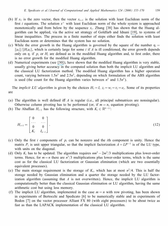
(b) The Aba�an Hi+1 has the following structure, with Ki ∈ Rn−i; i:

Hi+1 =

0 0· · · · · ·0 0Ki In−i

: (12)

(c) Only the �rst i components of pi can be nonzero and the ith component is unity. Hence thematrix Pi is unit upper triangular, so that the implicit factorization A= LP−1 is of the LU type,with units on the diagonal.

(d) Only Ki has to be updated. The algorithm requires nm2−2m3=3 multiplications plus lower-orderterms. Hence, for m=n there are n3=3 multiplications plus lower-order terms, which is the samecost as for the classical LU factorization or Gaussian elimination (which are two essentiallyequivalent processes).

(e) The main storage requirement is the storage of Ki, which has at most n2=4. This is half thestorage needed by Gaussian elimination and a quarter the storage needed by the LU factor-ization algorithm (assuming that A is not overwritten). Hence, the implicit LU algorithm iscomputationally better than the classical Gaussian elimination or LU algorithm, having the samearithmetic cost but using less memory.

(f) The implicit LU algorithm, implemented in the case m= n with row pivoting, has been shownin experiments of Bertocchi and Spedicato [6] to be numerically stable and in experiments ofBodon [7] on the vector processor Alliant FX 80 (with eight processors) to be about twice asfast as than the LAPACK implementation of the classical LU algorithm.

160 E. Spedicato et al. / Journal of Computational and Applied Mathematics 124 (2000) 155–170

The implicit LX algorithm is de�ned by the choices H1 = I; vi = ei; zi =wi = eki , where ki is aninteger, 16ki6n, such that

eTkiHiai 6= 0: (13)

Notice that by a general property of the ABS class for A with full rank there is at least one indexki such that (13) is satis�ed. For stability reasons it may be recommended to select ki such that�i = |eTkiHiai| is maximized. The following properties are valid for the implicit LX algorithm. Let Nbe the set of integers from 1 to n; N =(1; 2; : : : ; n). Let Bi be the set of indices k1; : : : ; ki chosen forthe parameters of the implicit LX algorithm up to the step i. Let Ni be the set N\Bi. Then

(a) The index ki is selected from Ni−1.(b) The rows of Hi+1 of index k ∈ Bi are null rows.(c) The vector pi has n− i zero components; its kith component is equal to one.(d) If x1 = 0, then xi+1 is a basic type solution of the �rst i equations, whose nonzero components

may lie only in the positions corresponding to the indices k ∈ Bi.(e) The columns of Hi+1 of index k ∈ Ni are the unit vectors ek , while the columns of Hi+1 of

index k ∈ Bi have zero components in the jth position, with j ∈ Bi, implying that only i(n− i)elements of such columns have to be computed.

(f) At the ith step i(n − i) multiplications are needed to compute Hiai and i(n − i) to update thenontrivial part of Hi. Hence the total number of multiplications is the same as for the implicitLU algorithm (i.e., n3=3), but no pivoting is necessary, re ecting the fact that no condition isrequired on the matrix A.

(g) The storage requirement is the same as for the implicit LU algorithm, i.e., at most n2=4. Hencethe implicit LX algorithm shares the same storage advantage of the implicit LU algorithm overthe classical LU algorithm, with the additional advantage of not requiring pivoting.

(h) Numerical experiments by Mirnia [23] have shown that the implicit LX method gives usuallybetter accuracy, in terms of error in the computed solution, than the implicit LU algorithm andoften even than the modi�ed Huang algorithm. In terms of size of the �nal residual, its accuracyis comparable to that of the LU algorithm as implemented (with row pivoting) in the MATLABor LAPACK libraries, but it is better again in terms of error in the solution.

4. Other ABS linear solvers and implementational details

ABS reformulations have been obtained for most algorithms proposed in the literature. The avail-ability of several formulations of the linear algebra of the ABS process allows alternative formulationsof each method, with possibly di�erent values of overhead, storage and di�erent properties of numer-ical stability, vectorization and parallelization. The reprojection technique, already seen in the caseof the modi�ed Huang algorithm and based upon the identities Hiq=Hi(Hiq); H T

i =HTi (H

Ti q), valid

for any vector q if H1 = I , remarkably improves the stability of the algorithm, the increase in thenumber of operations depending on the algorithm and the number of reprojections made. The ABSversions of the Hestenes–Stiefel and the Craig algorithms for instance are very stable under the abovereprojection. The implicit QR algorithm, de�ned by the choices H1 = I; vi=Api; zi=wi= ei can beimplemented in a very stable way using the reprojection in both the de�nition of the search vector

E. Spedicato et al. / Journal of Computational and Applied Mathematics 124 (2000) 155–170 161

and the scaling vector. It should also be noticed that the classical iterative re�nement procedure,which amounts to a Newton iteration on the system Ax− b= 0 using the approximate factors of A,can be reformulated in the ABS context using the previously de�ned search vectors pi. Experimentsof Mirnia [23] have shown that ABS re�nement works excellently.For problems with special structure ABS methods can often be implemented taking into account

the e�ect of the structure on the Aba�an matrix, which often tends to re ect the structure of thematrix A. Several cases of structured problems are discussed by Aba�y and Spedicato [4] and inlater papers. As an example, one can show that if A has a banded structure, the same is true forthe Aba�an matrix generated by the implicit LU, the implicit QR and the Huang algorithm, albeitthe band size is increased. If A is symmetric positive de�nite (SPD) and has a so-called nesteddissection (ND) structure, the same is true for the Aba�an matrix. In this case the implementationof the implicit LU algorithm uses much less storage, for large n, than the Choleski algorithm. Formatrices having the Kuhn–Tucker (KT) structure large classes of ABS methods have been developed,many of them better either in storage or in arithmetic cost than classical methods. For matrices withgeneral sparsity patterns little is presently known about minimizing the �ll-in in the Aba�an matrix.Careful use of BLAS4 routines can however substantially reduce the number of operations and makethe ABS implementation competitive with a sparse implementation of say the LU factorization (e.g.,by the code MA28) for values of n up to about 1000.It is possible to implement the ABS process also in block form, where several equations, instead

of just one, are dealt with at each step. The block formulation does not damage the numericalaccuracy and can lead to reduction of overhead on special problems or to faster implementations onvector or parallel computers.Finally, in�nite iterative methods can be obtained by the �nite ABS methods via two ways. The

�rst one involves restarting the iteration after k ¡m steps, so that the storage will be of order 2knif the representation of the Aba�an in terms of 2i vectors is used. The second approach uses only alimited number of terms in the Gram–Schmidt-type processes that are alternative formulations of theABS procedure. For both cases convergence at a linear rate has been established using the techniquedeveloped by Dennis and Turner [10]. The in�nite iteration methods obtained by these approachesde�ne a very large class of methods, that contains not only all Krylov-space-type methods of theliterature, but also non-Krylov-type methods such as the Gauss–Seidel, the De La Garza and theKackmartz methods, with their generalizations.

5. Applications to optimization; the unconstrained optimization case

We will now present some applications of ABS methods to optimization problems. In this sectionwe describe a class of ABS related methods for unconstrained optimization. In Section 6 we showhow ABS methods provide the general solution of the quasi-Newton equation, with sparsity andsymmetry conditions and we discuss how SPD solutions can be obtained. In Section 7 we presentseveral special ABS methods for solving the Kuhn–Tucker equations. In Section 8 we consider theapplication of the implicit LX algorithm to the linear programming (LP) problem. In Section 9 wepresent ABS approaches to the general linearly constrained optimization problem, which unify linearand nonlinear problems.

162 E. Spedicato et al. / Journal of Computational and Applied Mathematics 124 (2000) 155–170

ABS methods can be applied directly to the unconstrained minimization of a function f(x). Theyuse the iteration xi+1 = xi−�iH T

i zi, where Hi is reset after n or less steps and zi is chosen so that thedescent condition holds, i.e., gTi H

Ti zi ¿ 0, with gi = 3f(xi). If f(x) is quadratic, one can identify

the matrix A in the Aba�an update formula with the Hessian of f(x). De�ning a perturbed point x′

by x′ = xi − �vi one has on quadratic functions g′ = g− �Avi, and hence the update of the Aba�antakes the form Hi+1 = Hi − HiyiwTi Hi=wTi Hiyi, where yi = g′ − gi, so that no information is neededabout second derivatives. The above-de�ned class has termination on quadratic functions and localsuperlinear (n-step Q-quadratic) rate of convergence on general functions. It is a special case of aclass of projection methods developed by Psenichny and Danilin [25]. Almost no numerical resultsare available about the performance of the methods in this class.

6. Applications to quasi-Newton updates

ABS methods have been used to provide the general solution of the quasi-Newton equation, withthe additional conditions of symmetry, sparsity and positive de�niteness. While the general solutionof only the quasi-Newton equation has already been given by Adachi [5], the explicit formulasobtained for the sparse symmetric case are new, and so is the way of constructing sparse SPDupdates.Let us consider the transpose form of the quasi-Newton equation de�ning the new approximation

to a Jacobian or a Hessian

dTB′ = yT; (14)

where d= x′ − x; y= g′ − g. We observe that (14) can be seen as a set of n linear underdeterminedsystems, each one having just one equation and di�ering only on the right-hand side. Hence, thegeneral solution can be obtained by one step of the ABS method. It can be written in the followingway:

B′ = B− s(BTd− y)T=dTs+ (I − sdT=dTs)Q; (15)

where Q ∈ Rn;n is arbitrary, and s ∈ Rn is arbitrary subject to sTd 6= 0. Formula (15), derived bySpedicato and Xia [31], is equivalent to a formula of Adachi [5].Now the conditions that some elements of B′ should be zero, or have constant value or that B′

should be symmetric can be written as additional linear constraints. This if b′i is the ith column ofB′, we require

(b′i)Tek = �ij; (16)

where �ij = 0 implies sparsity, �ij = constant implies that some elements do not change their valueand �ij = �ji implies symmetry. The ABS algorithm can deal with these extra conditions. Spedicatoand Zhao [33] give the solution in explicit form, columnwise in presence of symmetry. By addingthe condition that the diagonal elements be su�ciently large, it is possible to obtain formulas whereB′ is quasi-positive de�nite or quasi-diagonally dominant, in the sense that the principal submatrixof order n − 1 is positive de�nite or diagonally dominant. It is not possible in general to forceB′ to be SPD, since SPD solutions may not exist, which is re ected in the fact that no additionalconditions can be put on the last diagonal element, since the last column is fully determined by then − 1 symmetry conditions and the quasi-Newton equation. This result can however be exploited

E. Spedicato et al. / Journal of Computational and Applied Mathematics 124 (2000) 155–170 163

to provide SPD approximations by imbedding the original minimization problem of n variables ina problem of n + 1 variables, whose solution with respect to the �rst n variables is the originalsolution. This imbedding modi�es the quasi-Newton equation so that SPD solutions exist. Numericalresults on the performance of the proposed sparse quasi-Newton methods are not yet available.

7. ABS methods for KT equations

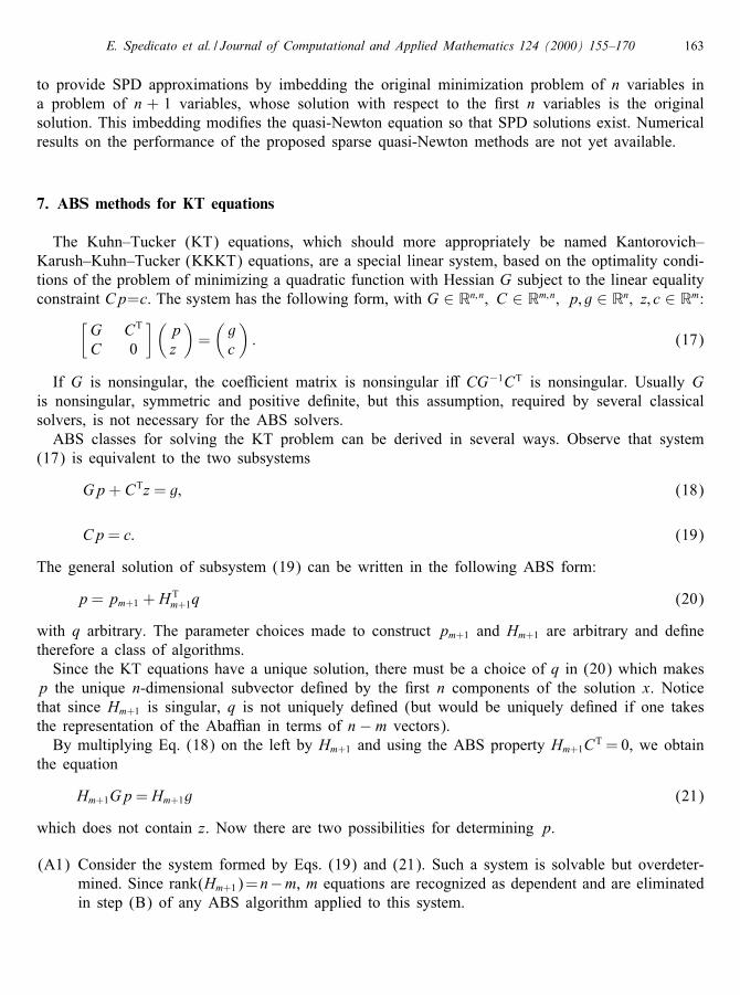
The Kuhn–Tucker (KT) equations, which should more appropriately be named Kantorovich–Karush–Kuhn–Tucker (KKKT) equations, are a special linear system, based on the optimality condi-tions of the problem of minimizing a quadratic function with Hessian G subject to the linear equalityconstraint Cp=c. The system has the following form, with G ∈ Rn;n; C ∈ Rm;n; p; g ∈ Rn; z; c ∈ Rm:

[G CT

C 0

](pz

)=

(gc

): (17)

If G is nonsingular, the coe�cient matrix is nonsingular i� CG−1CT is nonsingular. Usually Gis nonsingular, symmetric and positive de�nite, but this assumption, required by several classicalsolvers, is not necessary for the ABS solvers.ABS classes for solving the KT problem can be derived in several ways. Observe that system

(17) is equivalent to the two subsystems

Gp+ CTz = g; (18)

Cp= c: (19)

The general solution of subsystem (19) can be written in the following ABS form:

p= pm+1 + H Tm+1q (20)

with q arbitrary. The parameter choices made to construct pm+1 and Hm+1 are arbitrary and de�netherefore a class of algorithms.Since the KT equations have a unique solution, there must be a choice of q in (20) which makes

p the unique n-dimensional subvector de�ned by the �rst n components of the solution x. Noticethat since Hm+1 is singular, q is not uniquely de�ned (but would be uniquely de�ned if one takesthe representation of the Aba�an in terms of n− m vectors).By multiplying Eq. (18) on the left by Hm+1 and using the ABS property Hm+1CT = 0, we obtain

the equation

Hm+1Gp= Hm+1g (21)

which does not contain z. Now there are two possibilities for determining p.

(A1) Consider the system formed by Eqs. (19) and (21). Such a system is solvable but overdeter-mined. Since rank(Hm+1)=n−m, m equations are recognized as dependent and are eliminatedin step (B) of any ABS algorithm applied to this system.

164 E. Spedicato et al. / Journal of Computational and Applied Mathematics 124 (2000) 155–170

(A2) In Eq. (21) replace p by the general solution (20) to give

Hm+1GH Tm+1q= Hm+1g− Hm+1Gpm+1: (22)

The above system can be solved by any ABS method for a particular solution q, m equationsbeing again removed at step (B) of the ABS algorithm as linearly dependent.

Once p is determined, one can determine z in two ways, namely,

(B1) Solve by any ABS method the overdetermined compatible system

CTz = g− Gp (23)

by removing at step (B) of the ABS algorithm the (n− m)-dependent equations.(B2) Let P = (p1; : : : ; pm) be the matrix whose columns are the search vectors generated on the

system Cp= c. Now CP=L, with L nonsingular lower diagonal. Multiplying Eq. (23) on theleft by PT we obtain a triangular system, de�ning z uniquely as

LTz = PTg− PTGp: (24)

Extensive numerical testing has evaluated the accuracy of the above ABS algorithms for KT equationsfor certain choices of the ABS parameters (corresponding to the implicit LU algorithm with rowpivoting and the modi�ed Huang algorithm). The methods have been tested against classical methods,in particular the method of Aasen and methods using the QR factorization. The experiments haveshown that some ABS methods are the most accurate, in both residual and solution error; moreoversome ABS algorithms are cheaper in storage and in overhead, up to one order, especially for thecase when m is close to n. In particular, two methods based upon the implicit LU algorithm notonly have turned out to be more accurate, especially in residual error, than the method of Aasen andthe method using QR factorization via Houselder matrices, but they are also cheaper in number ofoperations (the method of Aasen has a lower storage for small m but a higher storage for large m).In many interior point methods the main computational cost is to compute the solution for a

sequence of KT problems where only G, which is diagonal, changes. In such a case the ABSmethods, which initially work on the matrix C, which is unchanged, have an advantage, particularlywhen m is large, where the dominant cubic term decreases with m and disappears for m = n, sothat the overhead is dominated by second-order terms. Again numerical experiments show that someABS methods are more accurate than the classical ones (for details see [28]).

8. Reformulation of the simplex method via the implicit LX algorithm

The implicit LX algorithm has a natural application to a reformulation of the simplex method forthe LP problem in standard form, i.e., the problem of minimizing cTx, subject to Ax = b; x¿0.The applicability of the implicit LX method is a consequence of the fact that the iterate xi+1

generated by the method, started from the zero vector, is a basic type vector, with a unit componentin the position ki. Nonidentically zero components correspond to indices j ∈ Bi, where Bi is theset of indices of the unit vectors chosen as the zi; wi parameters, i.e., the set Bi = (k1; : : : ; ki), whilethe components of xi+1 with indices in the set Ni = N=Bi are identically zero, where N = (1; : : : ; n).Therefore if the nonzero components are nonnegative, the point de�nes a vertex of the polytopecontaining the feasible points de�ned by the constraints of the LP problem.

E. Spedicato et al. / Journal of Computational and Applied Mathematics 124 (2000) 155–170 165

In the simplex method one moves from one vertex to another, according to some rules and usuallyreducing at each step the value of the function cTx. The direction along which one moves from onevertex to another is an edge direction of the polytope and is determined by solving a linear system,whose coe�cient matrix AB, the basic matrix, is de�ned by m linearly independent columns ofthe matrix A, called the basic columns. Usually such a system is solved by LU factorization oroccasionally by the QR method (see [14]). The new vertex is associated with a new basic matrixA′B, which is obtained by replacing one of the columns in AB by a column of the matrix AN , whichcomprises the columns of A that do not belong to AB. The most e�cient algorithm for solving themodi�ed system, after the column interchange, is the method of Forrest and Goldfarb [15], requiringm2 multiplications. Notice that the classical simplex method requires m2 storage for the matrix ABplus mn storage for the matrix A, which must be kept in general to provide the columns for theexchange.The application of the implicit LX method to the simplex method, developed by Xia [35], Zhang

and Xia [42], Spedicato et al. [32], Feng et al. [13], exploits the fact that in the implicit LX algorithmthe interchange of a jth column in AB with a kth column in AN corresponds to the interchange of apreviously chosen parameter vector zj=wj= ej with a new parameter zk =wk = ek . This operation isa special case of the perturbation of the Aba�an after a change in the parameters and can be doneusing a general formula of Zhang [39], without explicit use of the kth column in AN . Moreover,all quantities needed for the construction of the search direction (the edge direction) and for theinterchange criteria can as well be obtained without explicit use of the columns of A. Hence itfollows that the ABS approach needs only the storage of the matrix Hm+1, which, in the case ofthe implicit LX algorithm, is of size at most n2=4. Therefore, for values of m close to n the storagerequired by the ABS formulation is about 8 times less than for the classical simplex method.Here we give the basic formulae of the simplex method in both the classical and the ABS

formulation. The column in AN replacing an old column in AB is often taken as the column withminimal relative cost. In terms of the ABS formulation this is equivalent to minimizing the scalar�i = cTH Tei with respect to i ∈ Nm. Let N ∗ be the index chosen in this way. The column in ABto be exchanged is usually chosen with the criterion of the maximum displacement along an edgewhich keeps the basic variables nonnegative. De�ne !i= xTei=eTi H

TeN∗ , where x is the current basicfeasible solution. Then the above criterion is equivalent to minimizing !i with respect the set ofindices i ∈ Bm such that

eTi HTeN∗ ¿ 0: (25)

Notice that H TeN∗ 6= 0 and that an index i such that (25) is satis�ed always exists, unless x is asolution of the LP problem.The update of the Aba�an after the interchange of the unit vectors, which corresponds to the

update of the LU or QR factors after the interchange of the basic with the nonbasic column, is givenby the following formula:

H ′ = H − (HeB∗ − eB∗)eTN∗H=eTN∗HeB∗ : (26)

The search direction d, which in the classical formulation is obtained by solving the system ABd=−AeN∗ , is given by d = H T

m+1eN∗ , hence at no cost. Finally, the relative cost vector r, classicallygiven by r = c− ATA−1

B cB, where cB consists of the components of c with indices corresponding tothose of the basic columns, is simply given by r = Hm+1c.

166 E. Spedicato et al. / Journal of Computational and Applied Mathematics 124 (2000) 155–170

Let us now consider the computational cost of update (26). Since HeB∗ has at most n−m nonzerocomponents, while H TeN∗ has at most m, no more than m(n− m) multiplications are required. Theupdate is most expensive for m= n=2 and gets cheaper the smaller m is or the closer it is to n. Inthe dual steepest edge method of Forrest and Goldfarb [15] the overhead for replacing a column ism2, hence formula (26) is faster for m¿n=2 and is recommended on overhead considerations for msu�ciently large. However we notice that ABS updates having a O(m2) cost can also be obtainedby using the representation of the Aba�an in terms of 2m vectors. No computational experience hasbeen obtained till now on the new ABS formulation of the simplex method.Finally, a generalization of the simplex method, based upon the use of the Huang algorithm started

with a suitable singular matrix, has been developed by Zhang [40]. In this formulation the solution isapproached by points lying on a face of the polytope. Whenever the point hits a vertex the remainingiterates move among vertices and the method is reduced to the simplex method.

9. ABS uni�cation of feasible direction methods for minimization with linear constraints

ABS algorithms can be used to provide a uni�cation of feasible point methods for nonlinearminimization with linear constraints, including as a special case the LP problem. Let us �rst considerthe problem minf(x); x ∈ Rn, subject to Ax = b; A ∈ Rm;n; m6n; rank(A) = m.Let x1 be a feasible starting point. An iteration of the form xi+1 = xi − �idi, the search direction

will generate feasible points i�

Adi = 0: (27)

Solving the underdetermined system (27) for di by the ABS algorithm, the solution can be writtenin the following form, taking, without loss of generality, the zero vector as a special solution

di = H Tm+1q: (28)

Here the matrix Hm+1 depends on the arbitrary choice of the parameters H1, wi and vi used in solving(27) and q ∈ Rn is arbitrary. Hence the general feasible direction iteration has the form

xi+1 = xi − �iH Tm+1q: (29)

The search direction is a descent direction i� dT3f(x) = qTHm+13f(x)¿ 0. Such a condition canalways be satis�ed by choice of q unless Hm+13f(x)=0, which implies, from the null space structureof Hm+1, that 3f(x) = AT� for some �. In this case xi+1 is a KT point and � is the vector of theLagrange multipliers. When xi+1 is not a KT point, it is easy to see that the search direction is adescent directions if we select q by formula

q=WHm+13f(x)m; (30)

where W is a symmetric and positive-de�nite matrix.Particular well-known algorithms from the literature are obtained by the following choices of q,

with W = I :

(a) The reduced gradient method of Wolfe. Here Hm+1 is constructed by the implicit LU (or theimplicit LX) algorithm.

(b) The gradient projection method of Rosen. Here Hm+1 is built using the Huang algorithm.

E. Spedicato et al. / Journal of Computational and Applied Mathematics 124 (2000) 155–170 167

(c) The method of Goldfarb and Idnani. Here Hm+1 is built via the modi�cation of the Huangalgorithm where H1 is a symmetric positive de�nite matrix approximating the inverse Hessianof f(x).

Using the above ABS representations several formulations can be obtained of these classical algo-rithms, each one having in general di�erent storage requirements or arithmetic costs. No numericalexperience with such ABS methods is yet available but is expected that, similar to the case ofmethods for KKT equations, some of these formulations are better than the classical ones.If there are inequalities two approaches are possible.

(A) The active set approach. In this approach the set of linear equality constraints is modi�ed atevery iteration by adding and=or dropping some of the linear inequality constraints. Adding ordeleting a single constraint can be done, for every ABS algorithm, in order O(nm) operations(see [39]). In the ABS reformulation of the method of Goldfarb and Idnani [19] the initialmatrix is related to a quasi-Newton approximation of the Hessian and an e�cient update of theAba�an after a change in the initial matrix is discussed by Xia et al. [37].

(B) The standard form approach. In this approach, by introducing slack variables, the problemwith both types of linear constraints is written in the equivalent form minf(x), subject toAx = b; x¿0.

The following general iteration, started with a feasible point x1, generates a sequence of feasiblepoints for the problem in standard form

xi+1 = xi − �i�iHm+13f(x): (31)

In (30) the parameter �i can be chosen by a line search along the vector Hm+13f(x), while therelaxation parameter �i ¿ 0 is selected to prevent the new point having negative components.If f(x) is nonlinear, then Hm+1 can usually be determined once and for all at the �rst step, since

3f(x) generally changes from iteration to iteration and this will modify the search direction in (31)(unless the change in the gradient happens to be in the null space of Hm+1). If however f(x)=cTx islinear we must change Hm+1 in order to modify the search direction used in (31). As observed before,the simplex method is obtained by constructing Hm+1 with the implicit LX algorithm, every step ofthe method corresponding to a change of the parameters eki . It can be shown (see [36]), that themethod of Karmarkar (equivalent to an earlier method of Evtushenko [12]) corresponds to using thegeneralized Huang algorithm, with initial matrix H1 = Diag(xi) changing from iteration to iteration.Another method, faster than Karmarkar’s having superlinear against linear rate of convergence andO(

√n) against O(n) complexity, again �rst proposed by Evtushenko, is obtained by the generalized

Huang algorithm with initial matrix H1 = Diag(x2i ).

10. Final remarks and conclusions

In the above review we have given a partial presentation of the many results in the �eld of ABSmethods, documented in more than 350 papers. We have completely skipped the following topicswhere ABS methods have provided important results.

168 E. Spedicato et al. / Journal of Computational and Applied Mathematics 124 (2000) 155–170

(1) For linear least squares large classes of algorithms have been obtained; extensive numericalexperiments have shown that several ABS methods are more accurate than the QR-based codesavailable in standard libraries (see [26,27]).(2) For nonlinear algebraic equations ABS methods provide a generalization and include as special

cases both Newton and Brent methods (see [3]); they can be implemented using only, about halfof the Jacobian matrix, as is the case for Brent method (see [22,29]). Some of these methods havebetter global convergence properties than Newton method (see [16]), and they can keep a quadraticrate of convergence even if the Jacobian is singular at the solution (see [17]).(3) ABS methods have potential applications to the computation of eigenvalues (see [1]). Zhang

[41] particular deals with the computation of the inertia in KKT matrices, an important problem foralgorithms for the general quadratic programming problem using the active set strategy proposed byGould [20] and Gill et al. [18].(4) ABS methods can �nd a special integer solution and provide the set of all integer solutions

of a general Diophantine linear system (see [11]). The ABS approach to this problem providesinter alia an elegant characterization of the integer solvability of such a system that is a naturalgeneralization of the classical result well known for a single Diophantine equation in n variables.Work is on progress on using the ABS approach for 0–1 problems and integer solution of systemsof integer inequalities and integer LP.(5) Finally, work is in progress to develop and document ABSPACK, a package of ABS algorithms

for linear systems, linear least squares, nonlinear systems and several optimization problems. A �rstrelease of the package is expected in 2002.We think that the ABS approach, for reasons not to be discussed here still little known by

mathematicians, deserves to be more widely known and to be further developed in view of thefollowing undisputable achievements.(6) It provides a unifying framework for a large �eld of numerical methods, by itself an important

philosophical attainement.(7) Due to alternative formulations of the linear algebra of the ABS process, several implementa-

tions are possible of a given algorithm (here we identify an algorithm with the sequence of approx-imations to the solution that it generates in exact arithmetic), each one with possible advantages incertain circumstances.(8) Considerable numerical testing has shown many ABS methods to be preferable to more clas-

sical algorithms, justifying the interest in ABSPACK. We have solved real industrial problems usingABS methods where all other methods from commercial codes had failed.(9) It has led to the solution of some open problems in the literature, e.g., the explicit formulation

of sparse symmetric quasi-Newton updates. The implicit LX algorithm provides a general solver oflinear equations that is better than Gaussian elimination (same arithmetic cost, less intrinsic storage,regularity not needed) and that provides a much better implementation of the simplex method thanvia LU factorization for problems where the number of constraints is greater than half the numberof variables.The most interesting challenge to the power of ABS methods is whether by suitable choice of the

available parameters an elementary proof could be provided of Fermat’s last theorem in the contextof linear Diophantine systems.

E. Spedicato et al. / Journal of Computational and Applied Mathematics 124 (2000) 155–170 169

Acknowledgements

Work performed in the framework of a research supported partially by MURST Programma Co-�nanziato 1997.

References

[1] J. Aba�y, An ABS algorithm for general computation of eigenvalues, Communication, Second InternationalConference of ABS Methods, Beijing, June 1995.

[2] J. Aba�y, C.G. Broyden, E. Spedicato, A class of direct methods for linear systems, Numer. Math. 45 (1984)361–376.

[3] J. Aba�y, A. Galantai, E. Spedicato, The local convergence of ABS methods for non linear algebraic equations,Numer. Math. 51 (1987) 429–439.

[4] J. Aba�y, E. Spedicato, ABS Projection Algorithms: Mathematical Techniques for Linear and Nonlinear Equations,Ellis Horwood, Chichester, 1989.

[5] N. Adachi, On variable metric algorithms, J. Optim. Theory Appl. 7 (1971) 391–409.[6] M. Bertocchi, E. Spedicato, Performance of the implicit Gauss–Choleski algorithm of the ABS class on the IBM

3090 VF, Proceedings of the 10th Symposium on Algorithms, Strbske Pleso, 1989, pp. 30–40.[7] E. Bodon, Numerical experiments on the ABS algorithms for linear systems of equations, Report DMSIA 93=17,

University of Bergamo, 1993.[8] C.G. Broyden, On the numerical stability of Huang’s and related methods, J. Optim. Theory Appl. 47 (1985)

401–412.[9] J. Daniel, W.B. Gragg, L. Kaufman, G.W. Stewart, Reorthogonalized and stable algorithms for updating the Gram–

Schmidt QR factorization, Math. Comput. 30 (1976) 772–795.[10] J. Dennis, K. Turner, Generalized conjugate directions, Linear Algebra Appl. 88=89 (1987) 187–209.[11] H. Esmaeili, N. Mahdavi-Amiri, E. Spedicvato, Solution of Diophantine linear systems via the ABS methods, Report

DMSIA 99=29, University of Bergamo, 1999.[12] Y. Evtushenko, Two numerical methods of solving nonlinear programming problems, Sov. Dok. Akad. Nauk 251

(1974) 420–423.[13] E. Feng, X.M. Wang, X.L. Wang, On the application of the ABS algorithm to linear programming and linear

complementarity, Optim. Meth. Software 8 (1997) 133–142.[14] R. Fletcher, Dense factors of sparse matrices, in: A. Iserles, M.D. Buhmann (Eds.), Approximation Theory and

Optimization, Cambridge University Press, Cambridge, 1997, pp. 145–166.[15] J.J.H. Forrest, D. Goldfarb, Steepest edge simplex algorithms for linear programming, Math. Programming 57 (1992)

341–374.[16] A. Galantai, The global convergence of ABS methods for a class of nonlinear problems, Optim. Methods Software

4 (1995) 283–295.[17] R. Ge, Z. Xia, An ABS algorithm for solving singular nonlinear systems, Report DMSIA 36=96, University of

Bergamo, 1996.[18] P.E. Gill, W. Murray, M.A. Saunders, M.H. Wright, Inertia controlling methods for general quadratic programming,

SIAM Rev. 33 (1991) 1–36.[19] D. Goldfarb, A. Idnani, A numerically stable dual method for solving strictly convex quadratic programming, Math.

Program. 27 (1983) 1–33.[20] N.I.M. Gould, On practical conditions for the existence and uniqueness of solutions to the general equality quadratic

programming problem, Math. Programming 32 (1985) 90–99.[21] H.Y. Huang, A direct method for the general solution of a system of linear equations, J. Optim. Theory Appl. 16

(1975) 429–445.[22] A. Jeney, Discretization of a subclass of ABS methods for solving nonlinear systems of equations, Alkalmazott Mat.

Lapok 15 (1990) 353–364 (in Hungarian).

170 E. Spedicato et al. / Journal of Computational and Applied Mathematics 124 (2000) 155–170

[23] K. Mirnia, Numerical experiments with iterative re�nement of solutions of linear equations by ABS methods, ReportDMSIA 32=96, University of Bergamo, 1996.

[24] S. Nicolai, E. Spedicato, A bibliography of the ABS methods, Optim. Methods Software 8 (1997) 171–183.[25] B.N. Psenichny, Y.M. Danilin, Numerical Methods in Extremal Problems, MIR, Moscow, 1978.[26] E. Spedicato, E. Bodon, Numerical behaviour of the implicit QR algorithm in the ABS class for linear least squares,

Ric. Oper. 22 (1992) 43–55.[27] E. Spedicato, E. Bodon, Solution of linear least squares via the ABS algorithm, Math. Programming 58 (1993)

111–136.[28] E. Spedicato, Z. Chen, E. Bodon, ABS methods for KT equations, in: G. Di Pillo, F. Giannessi (Eds.), Nonlinear

Optimization and Applications, Plenum Press, New York, 1996, pp. 345–359.[29] E. Spedicato, Z. Chen, N. Deng, A class of di�erence ABS-type algorithms for a nonlinear system of equations,

Numer. Linear Algebra Appl. 13 (1994) 313–329.[30] E. Spedicato, M.T. Vespucci, Variations on the Gram–Schmidt and the Huang algorithms for linear systems: a

numerical study, Appl. Math. 2 (1993) 81–100.[31] E. Spedicato, Z. Xia, Finding general solutions of the quasi-Newton equation in the ABS approach, Optim. Methods

Software 1 (1992) 273–281.[32] E. Spedicato, Z. Xia, L. Zhang, Reformulation of the simplex algorithm via the ABS algorithm, preprint, University

of Bergamo, 1995.[33] E. Spedicato, J. Zhao, Explicit general solution of the quasi-Newton equation with sparsity and symmetry, Optim.

Methods Software 2 (1993) 311–319.[34] J.H.M. Wedderburn, Lectures on Matrices, Colloquium Publications, American Mathematical Society, New York,

1934.[35] Z. Xia, ABS reformulation of some versions of the simplex method for linear programming, Report DMSIA 10=95,

University of Bergamo, 1995.[36] Z. Xia, ABS generalization and formulation of the interior point method, preprint, University of Bergamo, 1995.[37] Z. Xia, Y. Liu, L. Zhang, Application of a representation of ABS updating matrices to linearly constrained

optimization, Northeast Oper. Res. 7 (1992) 1–9.[38] L. Zhang, An algorithm for the least Euclidean norm solution of a linear system of inequalities via the Huang ABS

algorithm and the Goldfarb–Idnani strategy, Report DMSIA 95=2, University of Bergamo, 1995.[39] L. Zhang, Updating of Aba�an matrices under perturbation in W and A, Report DMSIA 95=16, University of

Bergamo, 1995.[40] L. Zhang, On the ABS algorithm with singular initial matrix and its application to linear programming, Optim. Meth.

Software 8 (1997) 143–156.[41] L. Zhang, Computing inertias of KKT matrix and reduced Hessian via the ABS algorithm for applications to quadratic

programming, Report DMSIA 99=7, University of Bergamo, 1999.[42] L. Zhang, Z.H. Xia, Application of the implicit LX algorithm to the simplex method, Report DMSIA 9=95, University

of Bergamo, 1995.[43] L. Zhang, Z. Xia, E. Feng, Introduction to ABS Methods in Optimization, Dalian University of Technology Press,

Dalian, 1999 (in Chinese).