A NEW MARTIAN PALAEOPRESSURE CONSTRAINT

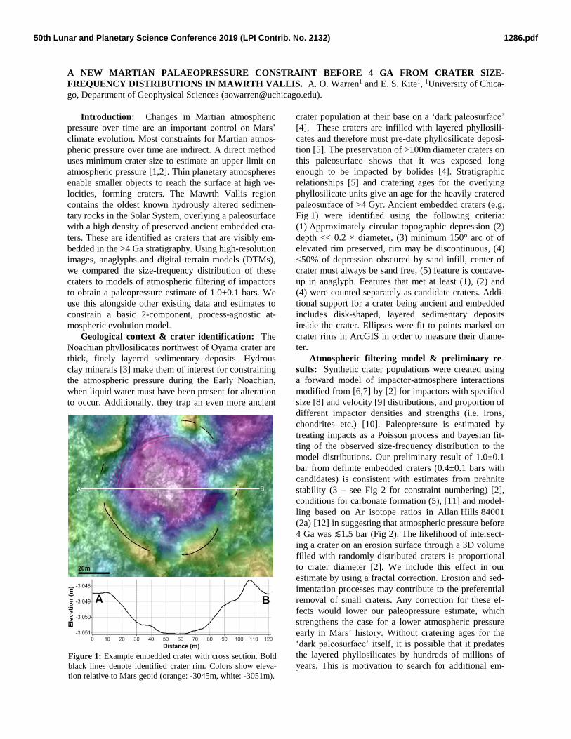
Figure 1: Example embedded crater with cross section. Bold

black lines denote identified crater rim. Colors show eleva-

tion relative to Mars geoid (orange: -3045m, white: -3051m).

B A

A NEW MARTIAN PALAEOPRESSURE CONSTRAINT BEFORE 4 GA FROM CRATER SIZE-

FREQUENCY DISTRIBUTIONS IN MAWRTH VALLIS. A. O. Warren1 and E. S. Kite1, 1University of Chica-

go, Department of Geophysical Sciences ([email protected]).

Introduction: Changes in Martian atmospheric

pressure over time are an important control on Mars’

climate evolution. Most constraints for Martian atmos-

pheric pressure over time are indirect. A direct method

uses minimum crater size to estimate an upper limit on

atmospheric pressure [1,2]. Thin planetary atmospheres

enable smaller objects to reach the surface at high ve-

locities, forming craters. The Mawrth Vallis region

contains the oldest known hydrously altered sedimen-

tary rocks in the Solar System, overlying a paleosurface

with a high density of preserved ancient embedded cra-

ters. These are identified as craters that are visibly em-

bedded in the >4 Ga stratigraphy. Using high-resolution

images, anaglyphs and digital terrain models (DTMs),

we compared the size-frequency distribution of these

craters to models of atmospheric filtering of impactors

to obtain a paleopressure estimate of 1.0±0.1 bars. We

use this alongside other existing data and estimates to

constrain a basic 2-component, process-agnostic at-

mospheric evolution model.

Geological context & crater identification: The

Noachian phyllosilicates northwest of Oyama crater are

thick, finely layered sedimentary deposits. Hydrous

clay minerals [3] make them of interest for constraining

the atmospheric pressure during the Early Noachian,

when liquid water must have been present for alteration

to occur. Additionally, they trap an even more ancient

crater population at their base on a ‘dark paleosurface’

[4]. These craters are infilled with layered phyllosili-

cates and therefore must pre-date phyllosilicate deposi-

tion [5]. The preservation of >100m diameter craters on

this paleosurface shows that it was exposed long

enough to be impacted by bolides [4]. Stratigraphic

relationships [5] and cratering ages for the overlying

phyllosilicate units give an age for the heavily cratered

paleosurface of >4 Gyr. Ancient embedded craters (e.g.

Fig 1) were identified using the following criteria:

(1) Approximately circular topographic depression (2)

depth << 0.2 × diameter, (3) minimum 150° arc of of

elevated rim preserved, rim may be discontinuous, (4)

<50% of depression obscured by sand infill, center of

crater must always be sand free, (5) feature is concave-

up in anaglyph. Features that met at least (1), (2) and

(4) were counted separately as candidate craters. Addi-

tional support for a crater being ancient and embedded

includes disk-shaped, layered sedimentary deposits

inside the crater. Ellipses were fit to points marked on

crater rims in ArcGIS in order to measure their diame-

ter.

Atmospheric filtering model & preliminary re-

sults: Synthetic crater populations were created using

a forward model of impactor-atmosphere interactions

modified from [6,7] by [2] for impactors with specified

size [8] and velocity [9] distributions, and proportion of

different impactor densities and strengths (i.e. irons,

chondrites etc.) [10]. Paleopressure is estimated by

treating impacts as a Poisson process and bayesian fit-

ting of the observed size-frequency distribution to the

model distributions. Our preliminary result of 1.0±0.1

bar from definite embedded craters (0.4±0.1 bars with

candidates) is consistent with estimates from prehnite

stability (3 – see Fig 2 for constraint numbering) [2],

conditions for carbonate formation (5), [11] and model-

ling based on Ar isotope ratios in Allan Hills 84001

(2a) [12] in suggesting that atmospheric pressure before

4 Ga was ≲1.5 bar (Fig 2). The likelihood of intersect-

ing a crater on an erosion surface through a 3D volume

filled with randomly distributed craters is proportional

to crater diameter [2]. We include this effect in our

estimate by using a fractal correction. Erosion and sed-

imentation processes may contribute to the preferential

removal of small craters. Any correction for these ef-

fects would lower our paleopressure estimate, which

strengthens the case for a lower atmospheric pressure

early in Mars’ history. Without cratering ages for the

‘dark paleosurface’ itself, it is possible that it predates

the layered phyllosilicates by hundreds of millions of

years. This is motivation to search for additional em-

1286.pdf50th Lunar and Planetary Science Conference 2019 (LPI Contrib. No. 2132)

Figure 3: Density of possible pressure evolution tracks for

four possible 2 component set-ups (constraints correspond

to Fig 2, red ‘x’ – this study). a) exponential source, expo-

nential sink, b) powerlaw source, exponential sink, c)

exponential source, powerlaw sink, d) powerlaw source,

powerlaw sink.

Figure 2: Mars paleopressure constraints (modified from

[2]). Direction of triangles indicates upper/lower bound. 1 –

cosmochemical estimate [13]. Black symbols – this study,

light blue - isotope-based models (2 [12], 4 [14], 6 [15])

yellow – mineralogical/thermodynamic constraints (3 [2], 5

[11]), grey – crater counting studies (8 [2]), orange - Gusev

bomb sag (7 [16]. 9 & 10 are modern CO2 inventory with

and without contributions from CO2 icecaps respectively.

bedded crater populations higher in the Mawrth stratig-

raphy. Our estimate suggests that at some point earlier

than 4 Ga Mars’ atmospheric pressure must have fallen

to 1.0±0.1 bar or below for long enough to accumulate

the observed embedded crater population. This could

be evidence for early escape of much of Mars’ primary

atmosphere, as suggested by the high 129Xe/132Xe ratio

of the present atmosphere [17]. This is evidence against

the hypothesis that a warm and wet early Mars can be

explained by retention of a thick, H2-rich proto-

atmosphere[18].

2-component atmospheric evolution model: The

atmospheric evolution of Mars depends on the relative

contributions of source and sink terms over time. De-

tailed evolution models rely on balancing fluxes from

processes such as impact delivery/erosion, outgassing,

and loss to space, for which many assumptions are nec-

essary. We used a basic 2-component model working

backwards from observed modern atmospheric pressure

(12 mbar if CO2 ice caps are included [19]) and meas-

ured MAVEN loss rates [20], gathering sources and

sinks into 1 term each. We choose to express these

terms as either a powerlaw (ΔPsource/sink = k1/3*t^(−k2/4))

or an exponential (ΔPsource/sink = k1/3*exp(−t/k2/4)) with

free parameters k1, k2 (sinks), k3 & k4 (sources), giving

4 possible source-sink set-ups (Fig 3). The parameters

{k1, k2,… k4} are found using the upper limits of exist-

ing paleopressure estimates (excluding 2b, 4 & 8b – Fig

2) as hard constraints to limit permitted pressure histo-

ries. The values of the parameters themselves are per-

haps less important than the array of possible pressure

evolutions (Fig 3). Existing data – including this study

– cannot rule out pressure histories that start with neg-

ligible atmospheres as late as 4.1 Ga, nor those that

experience atmospheric collapse (i.e. have permanent

ice caps) between ~3.6 Ga and just before present . Acknowledgements: J.-P. Williams wrote the

model of impactor-atmosphere interactions. J. Sneed

produced the HiRISE DTMs using the pipeline of [21].

Grants: NASA (NNX16AJ38G).

References: [1] Vasavada A. R. et al. (1993) JGR

Planets, 98, 3469-3479. [2] Kite E. et al. (2014) Nature

Geoscience, 7, 335-339. [3] Bishop J. L. et al. (2008)

Science, 321(5890), 830-833. [4] Loizeau D. et al.

(2010) Icarus, 205, 396-418. [5] Loizeau D. et al.

(2012) Planet. Space Sci. , 72(1), 31-43. [6] Williams

J. P. et al. (2014) Icarus, 235, 23-36. [7] Williams J. P.

& Pathare A. V. (2017) Meteoritics & Planetary Sci.,

53(4), 554-582. [8] Brown P. et al. (2002) Nature, 420,

294-296. [9] Davis P. (1993) Icarus, 225, 506-516.

[10] Ceplecha Z. et al. (1998) Space Sci Rev., 84, 327-

341 [11] Van Berk W. et al. (2012) J. Geophys. Res.,

117. [12] Cassata W. (2012) Earth and Planet. Sci.

Letters, 479, 322-329. [13] Lammer et al. (2013) Space

Sci. Rev., 174(1-4), 113-154. [14] Kurokawa et al.

(2018) Icarus, 299, 443-459. [15] Hu et al. (2015) Na-

ture Comm., 6:10003 [16] Manga et al. (2012) Ge-

ophys. Res. Lett., 39. [17] Conrad P. (2016) Earth

Planet. Sci. Lett., 454, 1-9. [18] Saito H. & Kuramoto

K. (2018) Monthly Notices of the Royal Astronomical

Soc., 475(1), 1274-1287. [19] Bierson C.J. et al. (2016)

Geophys. Res. Lett., 9, 4172-4179. [20] Lillis R. et al.

2017 Space Sci. Rev., 195, 357-422. [21] Mayer D.P.

& Kite E.S. (2016) LPSC XLVII, abstract #1241.


Can a Model of the Formation of the Solar System by Triggered Star Formation Within the Dense Shell of a Wolf-Rayet Bubble Explain the Initial Abundance of all Short-lived Radionuclides in the Early Solar System? V. V. Dwarkadas1, 1Department of Astronomy and Astrophysics, University of Chicago ([email protected]), N. Dauphas (University of Chicago), Meyer, B. (Clemson University).

Introduction: The early Solar System (ESS) was

characterized by a value of 26Al that exceeded the Ga-lactic average [1,2,3,4], while 60Fe in the ESS was about an order of magnitude less than the Galactic value [4,5]. These results disputed the existence of a supernova near the solar system at the time of formation. An alternative source of 26Al that has been suggested in the past is Wolf-Rayet (W-R) stars [5,6,7,8,9,10,11]. Aluminium-26 is carried out in the winds of these stars. No 60Fe is ejected in the wind, thus providing the necessary condi-tions for early solar system formation. In a recent paper, [12] showed that a single W-R star above about 50 M¤ could be sufficient to provide the measured amount of 26Al in the ESS. W-R stars have strong winds that sweep up the surrounding medium to form wind bubbles bor-dered by a dense shell. The 26Al is carried out by dust grains in the wind from the star to the dense shell, where it is released. The solar system could be formed by trig-gered star formation in the dense shell.

Besides 26Al and 60Fe, many other short-lived radio-nuclides (SLRs) were present in the ESS, including 10Be, 36Cl, 41Ca, 53Mn, 107Pd, 129I, and 182Hf [13,14]. In this paper, we investigate whether the triggered star-for-mation model can account for the abundance of all the short-lived radionuclides. In this model, the SLRs could be (1) emitted by the star, carried out in the wind (via dust grains in this model) and injected into the dense shell, (2) be already prevalent in the local interstellar medium that was swept-up to form the dense shell or (3) be due to irradiation, from the SN following the W-R star if a SN explosion occurs, or from the early Sun.

Short-lived radionuclides: A listing of short-lived radionuclides (SLRs) found in meteorites is given in [13, 14]. We investigate each SLR in turn.

10Be The abundance of this SLR is found to have a large range of values in meteorites. It also does not cor-relate with 26Al, which suggests a different source. It is most likely due to cosmic ray irradiation.

26Al Different stellar models provide varying amounts of 26Al. This can also vary depending on vari-ous factors such as stellar rotation, which are not in-cluded in all models. However, as was shown in [12], most stars above 50 M¤ can provide the level of 26Al seen in the ESS, even accounting for the fact that only 10% of the 26Al may eventually reach the dense shell.

36Cl Among the SLRs, this has a small half-life of about 300,000 yr. A recent estimate of 36Cl in the Al-lende CAI Curious Marie gives the ESS ratio of

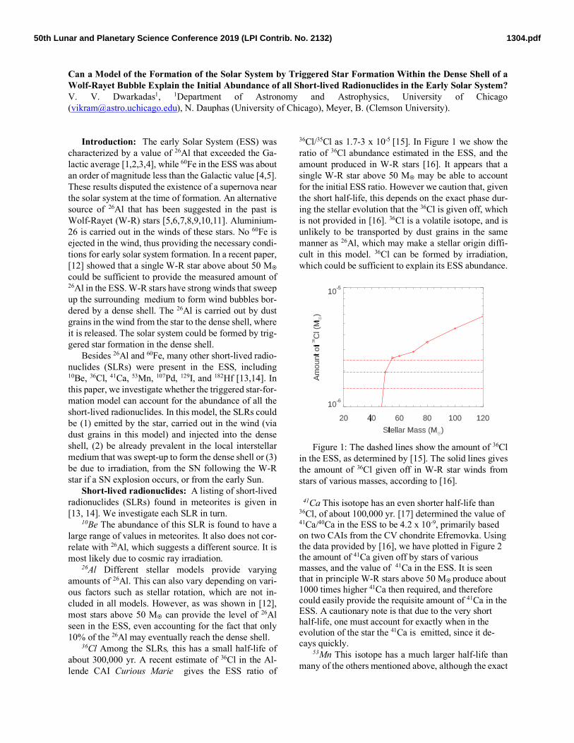
36Cl/35Cl as 1.7-3 x 10-5 [15]. In Figure 1 we show the ratio of 36Cl abundance estimated in the ESS, and the amount produced in W-R stars [16]. It appears that a single W-R star above 50 M¤ may be able to account for the initial ESS ratio. However we caution that, given the short half-life, this depends on the exact phase dur-ing the stellar evolution that the 36Cl is given off, which is not provided in [16]. 36Cl is a volatile isotope, and is unlikely to be transported by dust grains in the same manner as 26Al, which may make a stellar origin diffi-cult in this model. 36Cl can be formed by irradiation, which could be sufficient to explain its ESS abundance.

Figure 1: The dashed lines show the amount of 36Cl

in the ESS, as determined by [15]. The solid lines gives the amount of 36Cl given off in W-R star winds from stars of various masses, according to [16].

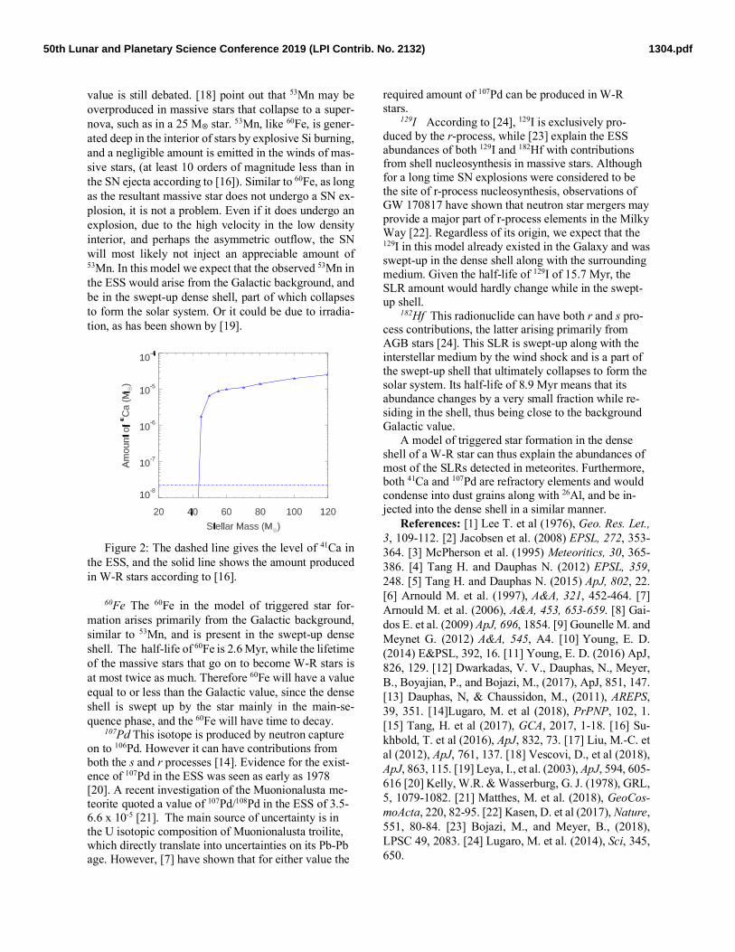
41Ca This isotope has an even shorter half-life than 36Cl, of about 100,000 yr. [17] determined the value of 41Ca/40Ca in the ESS to be 4.2 x 10-9, primarily based on two CAIs from the CV chondrite Efremovka. Using the data provided by [16], we have plotted in Figure 2 the amount of 41Ca given off by stars of various masses, and the value of 41Ca in the ESS. It is seen that in principle W-R stars above 50 M¤ produce about 1000 times higher 41Ca then required, and therefore could easily provide the requisite amount of 41Ca in the ESS. A cautionary note is that due to the very short half-life, one must account for exactly when in the evolution of the star the 41Ca is emitted, since it de-cays quickly.

53Mn This isotope has a much larger half-life than many of the others mentioned above, although the exact


value is still debated. [18] point out that 53Mn may be overproduced in massive stars that collapse to a super-nova, such as in a 25 M¤ star. 53Mn, like 60Fe, is gener-ated deep in the interior of stars by explosive Si burning, and a negligible amount is emitted in the winds of mas-sive stars, (at least 10 orders of magnitude less than in the SN ejecta according to [16]). Similar to 60Fe, as long as the resultant massive star does not undergo a SN ex-plosion, it is not a problem. Even if it does undergo an explosion, due to the high velocity in the low density interior, and perhaps the asymmetric outflow, the SN will most likely not inject an appreciable amount of 53Mn. In this model we expect that the observed 53Mn in the ESS would arise from the Galactic background, and be in the swept-up dense shell, part of which collapses to form the solar system. Or it could be due to irradia-tion, as has been shown by [19].

Figure 2: The dashed line gives the level of 41Ca in

the ESS, and the solid line shows the amount produced in W-R stars according to [16].

60Fe The 60Fe in the model of triggered star for-

mation arises primarily from the Galactic background, similar to 53Mn, and is present in the swept-up dense shell. The half-life of 60Fe is 2.6 Myr, while the lifetime of the massive stars that go on to become W-R stars is at most twice as much. Therefore 60Fe will have a value equal to or less than the Galactic value, since the dense shell is swept up by the star mainly in the main-se-quence phase, and the 60Fe will have time to decay.

107Pd This isotope is produced by neutron capture on to 106Pd. However it can have contributions from both the s and r processes [14]. Evidence for the exist-ence of 107Pd in the ESS was seen as early as 1978 [20]. A recent investigation of the Muonionalusta me-teorite quoted a value of 107Pd/108Pd in the ESS of 3.5-6.6 x 10-5 [21]. The main source of uncertainty is in the U isotopic composition of Muonionalusta troilite, which directly translate into uncertainties on its Pb-Pb age. However, [7] have shown that for either value the

required amount of 107Pd can be produced in W-R stars.

129I According to [24], 129I is exclusively pro-duced by the r-process, while [23] explain the ESS abundances of both 129I and 182Hf with contributions from shell nucleosynthesis in massive stars. Although for a long time SN explosions were considered to be the site of r-process nucleosynthesis, observations of GW 170817 have shown that neutron star mergers may provide a major part of r-process elements in the Milky Way [22]. Regardless of its origin, we expect that the 129I in this model already existed in the Galaxy and was swept-up in the dense shell along with the surrounding medium. Given the half-life of 129I of 15.7 Myr, the SLR amount would hardly change while in the swept-up shell.

182Hf This radionuclide can have both r and s pro-cess contributions, the latter arising primarily from AGB stars [24]. This SLR is swept-up along with the interstellar medium by the wind shock and is a part of the swept-up shell that ultimately collapses to form the solar system. Its half-life of 8.9 Myr means that its abundance changes by a very small fraction while re-siding in the shell, thus being close to the background Galactic value.

A model of triggered star formation in the dense shell of a W-R star can thus explain the abundances of most of the SLRs detected in meteorites. Furthermore, both 41Ca and 107Pd are refractory elements and would condense into dust grains along with 26Al, and be in-jected into the dense shell in a similar manner.

References: [1] Lee T. et al (1976), Geo. Res. Let., 3, 109-112. [2] Jacobsen et al. (2008) EPSL, 272, 353-364. [3] McPherson et al. (1995) Meteoritics, 30, 365-386. [4] Tang H. and Dauphas N. (2012) EPSL, 359, 248. [5] Tang H. and Dauphas N. (2015) ApJ, 802, 22. [6] Arnould M. et al. (1997), A&A, 321, 452-464. [7] Arnould M. et al. (2006), A&A, 453, 653-659. [8] Gai-dos E. et al. (2009) ApJ, 696, 1854. [9] Gounelle M. and Meynet G. (2012) A&A, 545, A4. [10] Young, E. D. (2014) E&PSL, 392, 16. [11] Young, E. D. (2016) ApJ, 826, 129. [12] Dwarkadas, V. V., Dauphas, N., Meyer, B., Boyajian, P., and Bojazi, M., (2017), ApJ, 851, 147. [13] Dauphas, N, & Chaussidon, M., (2011), AREPS, 39, 351. [14]Lugaro, M. et al (2018), PrPNP, 102, 1. [15] Tang, H. et al (2017), GCA, 2017, 1-18. [16] Su-khbold, T. et al (2016), ApJ, 832, 73. [17] Liu, M.-C. et al (2012), ApJ, 761, 137. [18] Vescovi, D., et al (2018), ApJ, 863, 115. [19] Leya, I., et al. (2003), ApJ, 594, 605-616 [20] Kelly, W.R. & Wasserburg, G. J. (1978), GRL, 5, 1079-1082. [21] Matthes, M. et al. (2018), GeoCos-moActa, 220, 82-95. [22] Kasen, D. et al (2017), Nature, 551, 80-84. [23] Bojazi, M., and Meyer, B., (2018), LPSC 49, 2083. [24] Lugaro, M. et al. (2014), Sci, 345, 650.


PRESOLAR SILICON CARBIDE GRAINS OF GROUPS Y AND Z: THEIR STRONTIUM AND BARIUM ISOTOPIC COMPOSITIONS AND STELLAR ORIGINS. N. Liu1,2, T. Stephan3, S. Cristallo4, R. Gallino5, P. Boehnke3, L. R. Nittler2, C. M. O’D. Alexander2, A. M. Davis3, R. Trappitsch6, and M. J. Pellin3,7, 1Department of Physics, Washington University in St. Louis, St. Louis, MO 63130, USA, [email protected], 2Department of Terrestrial Magnetism, Carnegie Institution for Science, Washington, DC 20015, USA, 3The University of Chicago, Chicago, IL 60637, USA, 4INAF-Osservatorio Astronomico d’Abruzzo, Teramo 64100, Italy, 5Dipartimento di Fisi-ca, Università di Torino, Torino 10125, Italy, 6Lawrence Livermore National Laboratory, CA 94550, USA, 7Argonne National Laboratory, Argonne, IL 60439, USA.

Introduction: Presolar Y and Z grains, ~1% each of the whole presolar SiC population, are believed to have come from asymptotic giant branch (AGB) stars with lower metallicities and perhaps larger masses with respect to mainstream (MS) grains, the dominant popu-lation of presolar SiC grains [1,2]. Type Y grains have 12C/13C>100 and are more 30Si-rich and 29Si-poor than MS grains. Z grains have 10<12C/13C<100, similar to MS grains, and are more 30Si-rich and 29Si-poor than Y grains. The definitions of these two rare groups are somewhat arbitrary, and there is considerable isotopic overlap between them and MS grains. In fact, the three groups of grains are indistinguishable in their 14N/15N and inferred 26Al/27Al ratios [3]. The conclusion that Y and Z grains came from AGB stars of about ½ Z

¤ and ⅓

Z¤

, respectively, relied mainly upon comparison with AGB model predictions to explain their large 30Si ex-cesses [2]. However, it was shown later that these low-metallicity models fail to consistently explain the Si and Ti isotope ratios of Y and Z grains [3]. Thus, the pro-posed low-metallicity stellar origin of Y and Z grains remains debatable.

To better understand the stellar origins of Y and Z grains, we obtained Sr, Mo, and Ba isotope data in a large number of new Y and Z grains with the Chicago Instrument for Laser Ionization (CHILI) [4]. Strontium, Mo, and Ba are significantly overproduced during the s-process, unlike Si; as a result, contributions from the initial abundances incorporated from the interstellar medium barely affect their s-process isotopic signatures generated during the AGB phase. Thus, the heavy-element isotope data from this study allow, for the first time, independent investigation of the s-process in the parent stars of Y and Z grains. The Mo isotope data [5,6] showed that the three groups of grains share com-parable Mo isotope ratios that are linearly correlated in the Mo 3-isotope plots, thus implying that the 95Zr branch remained inactive in their parent stars. Detailed data-model comparisons for Mo isotopes constrained the maximal temperature (TMAX) to lie below 3×108 K. Here we report the simultaneously obtained Sr and Ba isotope data, based on which we further discuss the s-process efficiency in their parent AGB stars.

Experiments & Models: We analyzed 37 sub-µm- to µm-sized Y and Z grains for their Sr, Mo, and Ba

isotopic compositions with CHILI [4]; 15 MS grains were also measured during the same session. These grains had been measured with the Carnegie NanoSIMS 50L ion microprobe for their C, N, and Si isotope ratios prior to the CHILI analyses. Molybdenum isotope ratios were obtained in all the 52 grains, while Sr and Ba iso-tope ratios were obtained in 36 and 22 out of the 52 grains, respectively.

Updated Torino models for AGB stars with metallic-ities between 0.5 Z

¤ to 1.5 Z

¤ have been recently pre-

sented [7,8]. In this study, we extend the metallicity down to 0.22 Z

¤. The updated nucleosynthesis calcula-

tions were conducted based on physical quantities ex-tracted from new FRUITY stellar models [9,10]. Com-pared to the FRANEC stellar models adopted in previ-ous Torino model calculations, the FRUITY stellar models predict higher third dredge-up efficiencies, low-er TMAX values, and higher mass-loss rates.

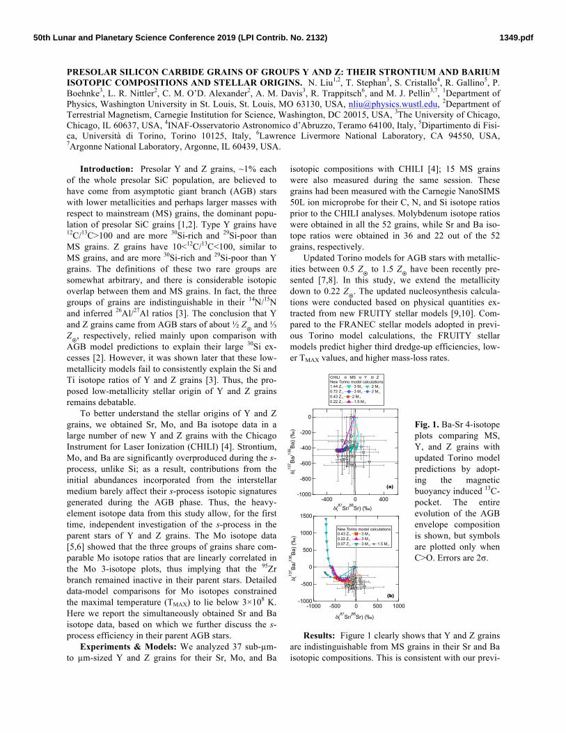
Fig. 1. Ba-Sr 4-isotope plots comparing MS, Y, and Z grains with updated Torino model predictions by adopt-ing the magnetic buoyancy induced 13C-pocket. The entire evolution of the AGB envelope composition is shown, but symbols are plotted only when C>O. Errors are 2σ.

Results: Figure 1 clearly shows that Y and Z grains are indistinguishable from MS grains in their Sr and Ba isotopic compositions. This is consistent with our previ-

-1000

-800

-600

-400

-200

0

δ(13

7 Ba/

136 B

a) (‰

)

-400 0 400δ(87Sr/88Sr) (‰)

1500

1000

500

0

-500

-1000

δ(13

7 Ba/

136 B

a) (‰

)

-1000 -500 0 500 1000

δ(87Sr/88Sr) (‰)

New Torino model calculations0.43 Z! 3 M!

0.22 Z! 3 M!

0.07 Z! 3 M! 1.5 M!

(a)

(b)

CHILI MS Y ZNew Torino model calculations1.44 Z! 3 M! 2 M!

0.72 Z! 3 M! 2 M!

0.43 Z! 2 M!

0.22 Z! 1.5 M!


ous observation that the three groups of grains share comparable Mo isotopic compositions [5,6]. Thus, our and literature data have shown that Y and Z grains over-lap with MS grains in the isotope ratios of N, Al, Ni [9], Sr, Zr [11], Mo, Ba and mainly show differences in Si and Ti [2,3].

Discussion: Figure 1b indicates large discrepancies in δ137Ba between the grain data and model predictions for AGB stars of high-mass and low-metallicity. This is because TMAX increases with both decreasing stellar metallicity and increasing stellar mass so that the 22Ne(α,n)25Mg reaction, the minor neutron source for the s-process in AGB stars, operates more efficiently to activate the branch point at 136Cs, thus resulting in en-hanced 137Ba production. The fact that TMAX values in all the models shown in Fig. 1b exceed 3×108 K further strengthens our previous constraint on TMAX (<3×108 K) based on the Mo isotope data, thus pointing to the low-mass and/or close-to-solar metallicity stellar origins of Y and Z grains.

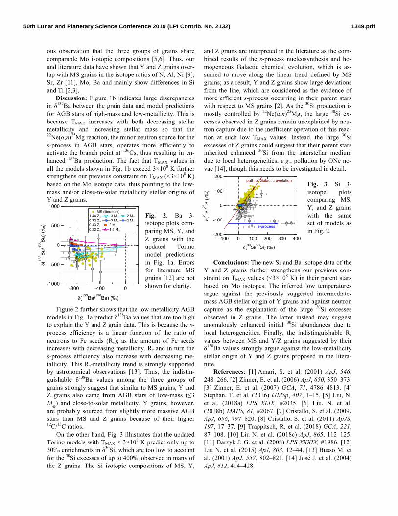
Fig. 2. Ba 3-isotope plots com-paring MS, Y, and Z grains with the updated Torino model predictions in Fig. 1a. Errors for literature MS grains [12] are not shown for clarity.

Figure 2 further shows that the low-metallicity AGB models in Fig. 1a predict δ138Ba values that are too high to explain the Y and Z grain data. This is because the s-process efficiency is a linear function of the ratio of neutrons to Fe seeds (Rs); as the amount of Fe seeds increases with decreasing metallicity, Rs and in turn the s-process efficiency also increase with decreasing me-tallicity. This Rs-metallicity trend is strongly supported by astronomical observations [13]. Thus, the indistin-guishable δ138Ba values among the three groups of grains strongly suggest that similar to MS grains, Y and Z grains also came from AGB stars of low-mass (≤3 M

¤) and close-to-solar metallicity. Y grains, however,

are probably sourced from slightly more massive AGB stars than MS and Z grains because of their higher 12C/13C ratios.

On the other hand, Fig. 3 illustrates that the updated Torino models with TMAX < 3×108 K predict only up to 30‰ enrichments in δ30Si, which are too low to account for the 30Si excesses of up to 400‰ observed in many of the Z grains. The Si isotopic compositions of MS, Y,

and Z grains are interpreted in the literature as the com-bined results of the s-process nucleosynthesis and ho-mogeneous Galactic chemical evolution, which is as-sumed to move along the linear trend defined by MS grains; as a result, Y and Z grains show large deviations from the line, which are considered as the evidence of more efficient s-process occurring in their parent stars with respect to MS grains [2]. As the 30Si production is mostly controlled by 22Ne(α,n)25Mg, the large 30Si ex-cesses observed in Z grains remain unexplained by neu-tron capture due to the inefficient operation of this reac-tion at such low TMAX values. Instead, the large 30Si excesses of Z grains could suggest that their parent stars inherited enhanced 30Si from the interstellar medium due to local heterogeneities, e.g., pollution by ONe no-vae [14], though this needs to be investigated in detail.

Fig. 3. Si 3-isotope plots comparing MS, Y, and Z grains with the same set of models as in Fig. 2.

Conclusions: The new Sr and Ba isotope data of the Y and Z grains further strengthens our previous con-straint on TMAX values (<3×108 K) in their parent stars based on Mo isotopes. The inferred low temperatures argue against the previously suggested intermediate-mass AGB stellar origin of Y grains and against neutron capture as the explanation of the large 30Si excesses observed in Z grains. The latter instead may suggest anomalously enhanced initial 30Si abundances due to local heterogeneities. Finally, the indistinguishable Rs values between MS and Y/Z grains suggested by their δ138Ba values strongly argue against the low-metallicity stellar origin of Y and Z grains proposed in the litera-ture.

References: [1] Amari, S. et al. (2001) ApJ, 546, 248–266. [2] Zinner, E. et al. (2006) ApJ, 650, 350–373. [3] Zinner, E. et al. (2007) GCA, 71, 4786–4813. [4] Stephan, T. et al. (2016) IJMSp, 407, 1–15. [5] Liu, N. et al. (2018a) LPS XLIX, #2035. [6] Liu, N. et al. (2018b) MAPS, 81, #2067. [7] Cristallo, S. et al. (2009) ApJ, 696, 797–820. [8] Cristallo, S. et al. (2011) ApJS, 197, 17–37. [9] Trappitsch, R. et al. (2018) GCA, 221, 87–108. [10] Liu N. et al. (2018c) ApJ, 865, 112–125. [11] Barzyk J. G. et al. (2008) LPS XXXIX, #1986. [12] Liu N. et al. (2015) ApJ, 803, 12–44. [13] Busso M. et al. (2001) ApJ, 557, 802–821. [14] José J. et al. (2004) ApJ, 612, 414–428.

-200

-100

0

100

200

δ(29

Si/28

Si)

(‰)

4003002001000-100

δ(30

Si/28

Si) (‰)

s-process

path of Galactic evolution

-1000

-500

0

500

1000

δ (13

8 Ba/

136 B

a) (‰

)

-800 -400 0

δ(135Ba/136Ba) (‰)

MS (literature)1.44 Z! 3 M! 2 M!

0.72 Z! 3 M! 2 M!

0.43 Z! 2 M!

0.22 Z! 1.5 M!


ARIDITY ENABLES WARM CLIMATES ON MARS.

Edwin S. Kite1 ([email protected]), Liam J. Steele

1,2, Michael A. Mischna

2

1. University of Chicago. 2. Jet Propulsion Laboratory, NASA/Caltech.

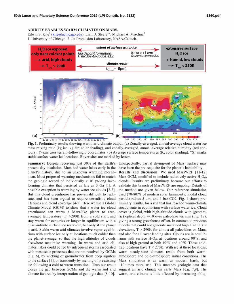
Fig. 1. Preliminary results showing warm, arid climate output. (a) Zonally-averaged, annual-average cloud water ice

mass mixing ratio (kg ice: kg air; color shading), and zonally-averaged, annual-average relative humidity (red con-

tours). Y-axis uses terrain-following σ coordinates. (b) Average surface temperatures (K; color shading). “X” marks

stable surface water ice locations. Rover sites are marked by letters.

Summary: Despite receiving just 30% of the Earth’s

present-day insolation, Mars had water lakes early in the

planet‘s history, due to an unknown warming mecha-

nism. Most proposed warming mechanisms fail to match

the geologic record of individually >102 yr-long lake-

forming climates that persisted as late as 3 Ga [1]. A

possible exception is warming by water ice clouds [2-3].

But this cloud greenhouse has proven difficult to repli-

cate, and has been argued to require unrealistic cloud

lifetimes and cloud coverage [4-5]. Here we use a Global

Climate Model (GCM) to show that a water ice cloud

greenhouse can warm a Mars-like planet to area-

averaged temperature (T) >290K from a cold start, and

stay warm for centuries or longer in equilibrium with a

quasi-infinite surface ice reservoir, but only if the planet

is arid. Stable warm arid climates involve vapor equilib-

rium with surface ice only at locations much colder than

the planet-average, so that the high altitudes of clouds

elsewhere maximize warming. In warm and arid cli-

mates, lakes could be fed by infrequent storms associated

with mesoscale processes that are not resolved by GCMs

(e.g. 6), by wicking of groundwater from deep aquifers

to the surface [7], or transiently by melting of preexisting

ice following a cold-to-warm transition. Thus our result

closes the gap between GCMs and the warm and arid

climate favored by interpretation of geologic data [8-10].

Unexpectedly, partial drying-out of Mars’ surface may

have been the pre-requisite for the planet’s habitability.

Results and discussion: We used MarsWRF [11-12]

Mars GCM, modified to include radiatively-active H2O(i)

clouds. Results are preliminary because our efforts to

validate this branch of MarsWRF are ongoing. Details of

the method are given below. Our reference simulation

used (70-80)% of modern solar luminosity, modal cloud

particle radius 5 µm, and 1 bar CO2. Fig. 1 shows pre-

liminary results, for a run that has reached warm-climate

steady-state in equilibrium with surface water ice. Cloud

cover is global, with high-altitude clouds with (geomet-

ric) optical depth 4-10 over paleolake terrains (Fig. 1a),

giving a strong greenhouse effect. In contrast to previous

models that could not generate sustained high T at +1 km

elevations, T > 290K for almost all paleolakes on Mars,

and also for all rover landing sites. Clouds are in equilib-

rium with surface H2O(i) at locations around 90°S, and

also at high ground at both 40°N and 40°S. These cold-

trap locations have T < 270K. With ice at these locations,

warm steady-state climates result from both warm-

atmosphere and cold-atmosphere initial conditions. The

Mars simulation is as warm as modern Earth, but

~10 times more arid. This matches geologic data that

suggest an arid climate on early Mars [e.g. 7,9]. The

warm, arid climate is little-affected by increasing obliq-


uity from 0° to 25°, increasing eccentricity to 0.1, or

removing Olympus Mons.

Aridity is set by the distribution of perennial surface-

exposed H2O (water or ice). H2O is a greenhouse gas,

and H2O(i) clouds provide strong warming in Fig. 1.

Thus it is surprising that more extensive initial surface

H2O(i) distributions lead to <235K (Fig. 2). This is not a

surface albedo effect. Instead, cold-start runs initialized

with water ice in higher-T locations (e.g. S pole ice ex-

tending to 60°S, frozen Northern Ocean, or ice at >1 km

elevation) yield low-lying clouds that (for 70% of mod-

ern solar luminosity) produce net cooling. Thus, steady-

state climate warmth depends on aridity. Aridity increas-

es as the temperature difference (ΔTa-c) between typical

surface temperature Ta and cold trap surface temperature

Tc increases. This is because, for lower surface relative

humidity (at fixed surface temperature), moisture must

be lifted higher to condense and form clouds. As a result,

total cloud optical depth is less, and more sunlight reach-

es the surface. However, so long as the cloud has IR op-

tical depth τIR > 1, the greenhouse effect remains strong.

(An idealized MATLAB model of the cloud greenhouse

– with all atmospheric constituents radiatively inert ex-

cept for clouds – allows us to explore the control of

aridity, surface temperature, cloud structure, e.t.c. on the

strength of the cloud greenhouse effect.) Aridity is set by

the temperature difference (ΔTa-c) between typical sur-

face temperature Ta and the surface temperature of cold-

traps, Tc. What sets ΔTa-c? Growth of a tall mountain will

create cold ground at high elevation, which may increase

ΔTa-c. A thinner atmosphere, or a fall in obliquity, will

lead to a steeper equator-to-pole temperature gradient,

which can also increase ΔTa-c. Loss of surface H2O (e.g.

escape-to-space, hydration reactions, loss to deep aqui-

fers, or formation of lag deposits) will reduce the tenden-

cy of surface ice to be found away from the cold-trap

location. Each effect can make the planet more arid, and

thus bring a potential for warmer climate.

Details of method: We ran MarsWRF at 5.625° x 3.75°

horizontal resolution (40 vertical resolution levels). CO2

radiative transfer uses the Hadley model modified to use

a correlated-k scheme. H2O(i) particle radii are affected

by the number density (n) of cloud condensation nuclei

(CCN). Early Mars ‘n’ depends on the relative efficiency

of dust aerosol production by wind erosion versus dust

aerosol consumption via sediment induration, and is un-

known. To take account of this unknown, we considered

modal water ice cloud particle radii of 2.5 µm, 5 µm, and

10 µm. (Current low-latitude Mars H2O(i) particle radii

are 3-4 µm). Particles undergo slip-corrected Stokes set-

tling. To represent mass transfer from slow-settling cloud

particles to fast-settling snow (autoconversion), we in-

crease settling rate to 1 m/s when cloud particle density

exceeds 3 × 10-5

kg/kg. In our runs, cloud particles are

destroyed by downwards advection and particle settling

that leads to the particles re-evaporating as fall streaks,

typically 30 km above the surface. Surface thermal iner-

tia is constant (250 J m-2

K-1

s-1/2

) and surface albedo is

set to 0.2, except where substantial water ice exists, for

which surface albedo is set to 0.45. During the run,

which can last for ~102 simulated years (for cold-start

runs), the location of the surface H2O(i) can shift. A large

surface H2O(i) source is prescribed at t=0; its location

varies between runs and is a major control on the climate

outcome. Such equilibrium with a quasi-infinite surface

water source is a requirement for any habitable warm-

Mars climate mechanism.

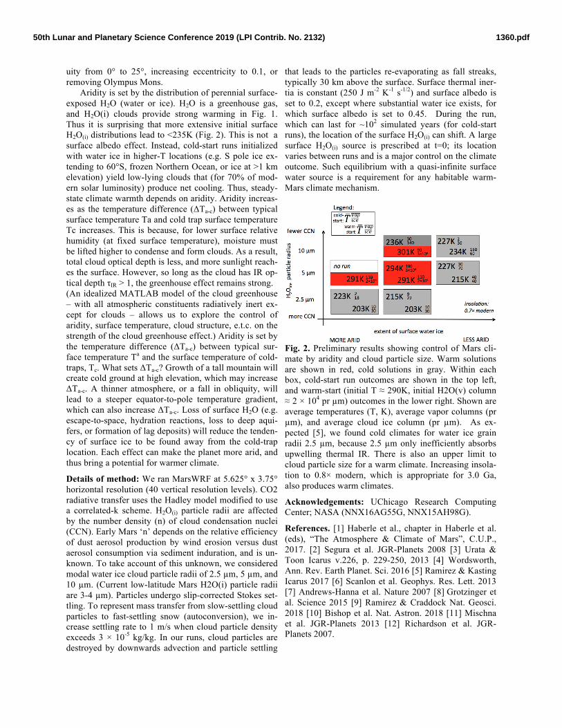
Fig. 2. Preliminary results showing control of Mars cli-

mate by aridity and cloud particle size. Warm solutions

are shown in red, cold solutions in gray. Within each

box, cold-start run outcomes are shown in the top left,

and warm-start (initial T ≈ 290K, initial H2O(v) column

≈ 2 × 104 pr µm) outcomes in the lower right. Shown are

average temperatures (T, K), average vapor columns (pr

µm), and average cloud ice column (pr µm). As ex-

pected [5], we found cold climates for water ice grain

radii 2.5 µm, because 2.5 µm only inefficiently absorbs

upwelling thermal IR. There is also an upper limit to

cloud particle size for a warm climate. Increasing insola-

tion to 0.8× modern, which is appropriate for 3.0 Ga,

also produces warm climates.

Acknowledgements: UChicago Research Computing

Center; NASA (NNX16AG55G, NNX15AH98G).

References. [1] Haberle et al., chapter in Haberle et al.

(eds), “The Atmosphere & Climate of Mars”, C.U.P.,

2017. [2] Segura et al. JGR-Planets 2008 [3] Urata &

Toon Icarus v.226, p. 229-250, 2013 [4] Wordsworth,

Ann. Rev. Earth Planet. Sci. 2016 [5] Ramirez & Kasting

Icarus 2017 [6] Scanlon et al. Geophys. Res. Lett. 2013

[7] Andrews-Hanna et al. Nature 2007 [8] Grotzinger et

al. Science 2015 [9] Ramirez & Craddock Nat. Geosci.

2018 [10] Bishop et al. Nat. Astron. 2018 [11] Mischna

et al. JGR-Planets 2013 [12] Richardson et al. JGR-

Planets 2007.


REASSESSING THE DEPLETIONS IN K AND Rb OF PLANETARY BODIES. N. Dauphas1. 1Origins La-boratory, Department of the Geophysical Sciences and Enrico Fermi Institute, The University of Chicago, Chicago IL, USA ([email protected]).

Introduction: Planetary bodies are variably de-

pleted in moderately volatile elements (MVE), includ-ing K and Rb [1-3]. The extent to which those depletions reflect nebular (incomplete condensation or evapora-tion) or planetary processes (impact-induced evapora-tion) is uncertain. Isotopic analyses of K and Rb have provided new insights into the processes that controlled the depletions in those elements [4-6] but significant questions remain. The degree of depletion for these ele-ments in large planetary bodies such as Earth, Moon, Mars, or Vesta, is not straightforward to assess because these bodies have experienced magmatic differentiation and the compositions of the rocks exposed at the surface of a planetary body are not necessarily representative its bulk composition. The degree of depletion in moder-ately volatile elements K and Rb is traditionally as-sessed by taking the ratio of those elements to another lithophile element of similar incompatibility but which is refractory rather than volatile [3 and references therein]. Uranium has been used for K normalization be-cause both elements are often reported in rock analyses and those two elements can be measured remotely by space probes. For example, the MESSENGER mission constrained the K/U ratio of the surface of Mercury to a value that is ~4.4 times lower than CI chondrites [7]. Strontium has been used for Rb normalization because those two elements are part of a radioactive decay sys-tem (87Rb-87Sr; t1/2=49 Gyr) and high-precision Rb/Sr ratios are available in the literature. By examining K/U and Rb/Sr ratios, Davis [3] established a relative scale of MVE depletion among planetary bodies. Knowing precisely the level of depletions in K and Rb, and the K/Rb ratios of planetary bodies is critical to develop a quantitative understanding of the processes that gave rise to those fractionations. For this reason, I have reas-sessed the abundances of K and Rb in planetary bodies, taking advantage of the large amount of concentration data available in the literature. Below, I focus on the de-pletions of K and Rb in the Moon relative to the Earth, as they are key constraints to scenarios of lunar for-mation [8-10].

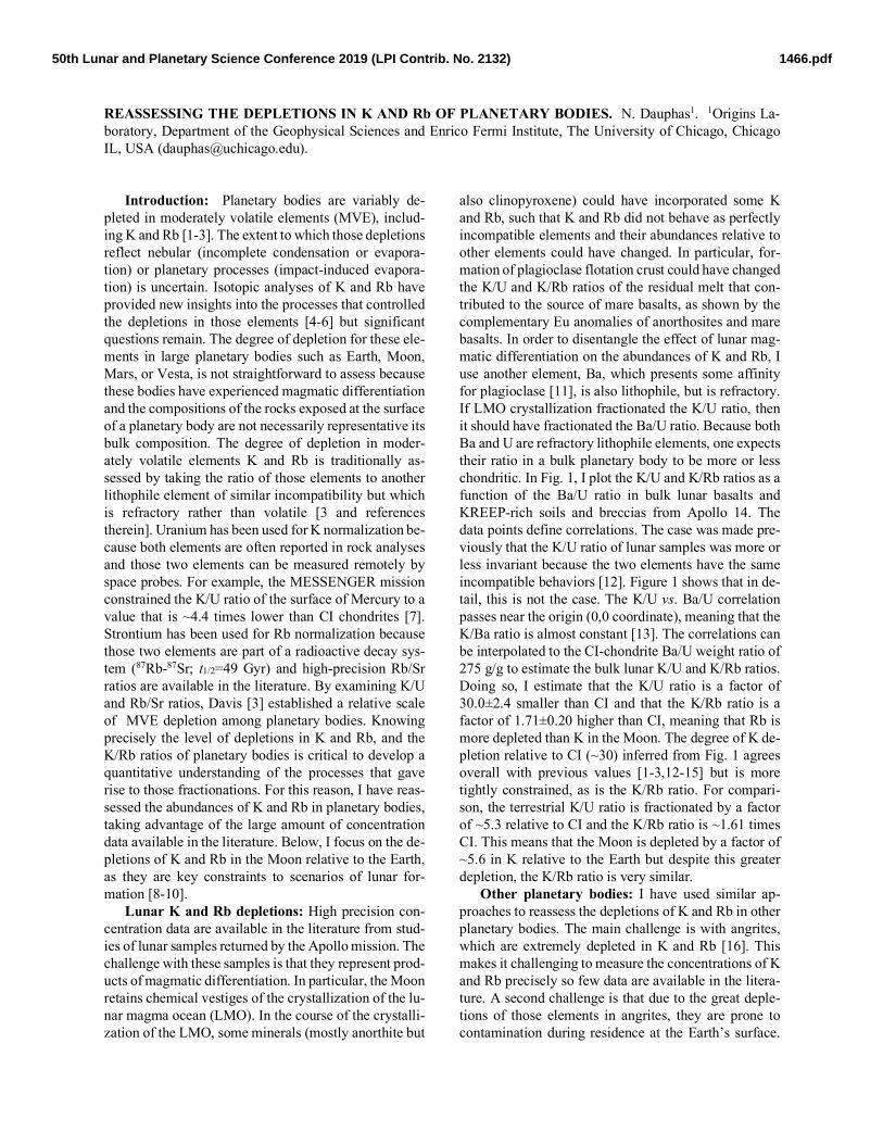
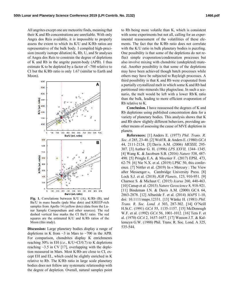
Lunar K and Rb depletions: High precision con-centration data are available in the literature from stud-ies of lunar samples returned by the Apollo mission. The challenge with these samples is that they represent prod-ucts of magmatic differentiation. In particular, the Moon retains chemical vestiges of the crystallization of the lu-nar magma ocean (LMO). In the course of the crystalli-zation of the LMO, some minerals (mostly anorthite but

also clinopyroxene) could have incorporated some K and Rb, such that K and Rb did not behave as perfectly incompatible elements and their abundances relative to other elements could have changed. In particular, for-mation of plagioclase flotation crust could have changed the K/U and K/Rb ratios of the residual melt that con-tributed to the source of mare basalts, as shown by the complementary Eu anomalies of anorthosites and mare basalts. In order to disentangle the effect of lunar mag-matic differentiation on the abundances of K and Rb, I use another element, Ba, which presents some affinity for plagioclase [11], is also lithophile, but is refractory. If LMO crystallization fractionated the K/U ratio, then it should have fractionated the Ba/U ratio. Because both Ba and U are refractory lithophile elements, one expects their ratio in a bulk planetary body to be more or less chondritic. In Fig. 1, I plot the K/U and K/Rb ratios as a function of the Ba/U ratio in bulk lunar basalts and KREEP-rich soils and breccias from Apollo 14. The data points define correlations. The case was made pre-viously that the K/U ratio of lunar samples was more or less invariant because the two elements have the same incompatible behaviors [12]. Figure 1 shows that in de-tail, this is not the case. The K/U vs. Ba/U correlation passes near the origin (0,0 coordinate), meaning that the K/Ba ratio is almost constant [13]. The correlations can be interpolated to the CI-chondrite Ba/U weight ratio of 275 g/g to estimate the bulk lunar K/U and K/Rb ratios. Doing so, I estimate that the K/U ratio is a factor of 30.0±2.4 smaller than CI and that the K/Rb ratio is a factor of 1.71±0.20 higher than CI, meaning that Rb is more depleted than K in the Moon. The degree of K de-pletion relative to CI (~30) inferred from Fig. 1 agrees overall with previous values [1-3,12-15] but is more tightly constrained, as is the K/Rb ratio. For compari-son, the terrestrial K/U ratio is fractionated by a factor of ~5.3 relative to CI and the K/Rb ratio is ~1.61 times CI. This means that the Moon is depleted by a factor of ~5.6 in K relative to the Earth but despite this greater depletion, the K/Rb ratio is very similar.

Other planetary bodies: I have used similar ap-proaches to reassess the depletions of K and Rb in other planetary bodies. The main challenge is with angrites, which are extremely depleted in K and Rb [16]. This makes it challenging to measure the concentrations of K and Rb precisely so few data are available in the litera-ture. A second challenge is that due to the great deple-tions of those elements in angrites, they are prone to contamination during residence at the Earth’s surface.


All angrites except one are meteorite finds, meaning that their K and Rb concentrations are unreliable. With only Angra dos Reis available, it is impossible to properly assess the extent to which its K/U and K/Rb ratios are representative of the bulk body. I compiled high-preci-sion (mostly isotope dilution) K, Rb, U, and Sr analyses of Angra dos Reis to constrain the degree of depletions of K and Rb in the angrite parent-body (APB). I thus estimate K to be depleted by a factor of ~700 relative to CI but the K/Rb ratio is only 1.67 (similar to Earth and Moon).

Discussion: Large planetary bodies display a range of depletions in K from ~3 in Mars to ~700 in the APB. For comparison, chondrites display K enrichments reaching 30% in EH (i.e., K/U=CI/0.7) to K depletions reaching ~3.5 in CV [17], overlapping with the deple-tion measured in Mars. Most K/Rb are close to CI, ex-cept EH and EL, which could be slightly enriched in K relative to Rb. The K/Rb ratio in large scale planetary bodies does not follow any systematic relationship with the degree of depletion. Overall, natural samples point

to Rb being more volatile than K, which is consistent with some experiments but not all, calling for an exper-imental reassessment of the volatilities of these ele-ments. The fact that the K/Rb ratio does not correlate with the K/U ratio in bulk planetary bodies is puzzling. One possibility is that some of the depletions do not re-flect simple evaporation/condensation processes but also involve mixing with chondritic (undepleted) mate-rial. Another possibility is that some of the depletions may have been achieved though batch processes while others may have be subjected to Rayleigh processes. A third possibility is that K and Rb were evaporated from a partially crystallized melt in which some K and Rb had partitioned into minerals like plagioclase. In such a sce-nario, the melt would be left with a lower Rb/K ratio than the bulk, leading to more efficient evaporation of Rb relative to K.

Conclusion. I have reassessed the degrees of K and Rb depletions using published concentration data for a variety of planetary bodies. This analysis shows that K and Rb show slightly different behaviors, providing an-other means of assessing the cause of MVE depletion in planets.

References: [1] Anders E. (1977) Phil. Trans. R. Soc. A 285, 23-40. [2] Wolf R. & Anders E. (1980) GCA 44, 2111-2124. [3] Davis A.M. (2006) MESSII, 295-307. [3] Author G. H. (1996) LPS XXVII, 1344–1345. [4] Wang K. & Jacobsen S.B. (2016) Nature 538, 487-490. [5] Pringle E.A. & Moynier F. (2017) EPSL 473, 62-79. [6] Nie N.X. et al. (2019) LPSC 50, this confer-ence. [7] Nittler et al. (2019) In « Mercury : The View after Messenger », Cambridge University Press. [8] Lock S.J. et al. (2018) JGR Planets, 123, 910-951. [9] Charnoz S. & Michaut C. (2015) Icarus 260, 440-463. [10] Canup et al. (2015) Nature Geoscience 8, 918-921. [11] Bindeman I.N. & Davis A.M. (2000) GCA 64, 2863-2878. [12] Albarède F. et al. (2014) MAPS 1-10, doi: 10.1111/maps.12331. [13] Wänke H. (1981) Phil. Trans. R. Soc. Lond. A 303, 287-302. [14] O’Neill H.St.C. (1991) GCA 55, 1135-1157. [15] McDonough W.F. et al. (1992) GCA 56, 1001-1012. [16] Tera F. et al. (1970) GCA 2, 1637-1657. [17] Wasson J.T. & Kal-lemeyn G.W. (1988) Phil. Trans. R. Soc. Lond. A 325, 535-544.

Fig. 1. Correlations between K/U (A), K/Rb (B), and Ba/U in mare basalts (pale blue dots) and KREEP-rich samples from Apollo 14 (yellow dots) (data from the Lu-nar Sample Compendium and other sources). The red dashed vertical line marks the CI Ba/U ratio. The red squares are the estimated K/U and K/Rb ratios of the Moon (this study).


REDETERMINING THE KINETICS OF FERROUS IRON PHOTO-OXIDATION UNDER UV FLUXES

RELEVANT TO EARLY MARS AND EARTH. A. W. Heard1, and N. Dauphas1. 1Origins Laboratory, Depart-

ment of the Geophysical Sciences and Enrico Fermi Institute, The University of Chicago, 5734 South Ellis Avenue,

Chicago, IL 60637, United States ([email protected]).

Introduction: Iron (Fe) plays an important role in

regulating the oxidation state of planetary surfaces be-

cause of its multiple redox states. On Mars, and Earth,

igneous rocks contain mostly reduced, ferrous Fe

(Fe2+). During weathering of the Fe-rich igneous crust,

Fe2+ is soluble, and if the surface environment is suffi-

ciently reducing, this Fe2+ can accumulate in standing

water bodies and aquifers. Evidence for these Fe-rich

and reducing – ‘ferruginous’ – conditions is common

through early Earth history, and they have also been

inferred for deeper facies of a redox-stratified Gale

Crater Lake on Mars [1]. Dissolved Fe2+ can be oxi-

dized to ferric iron (Fe3+), which tends to form insolu-

ble minerals that deposit as chemical sediments. When

Fe2+ oxidation is not coupled to any form of biological

carbon fixation, net oxidation of surface Fe is most

often balanced, directly or indirectly, by the formation

of H2 from water, and this H2 can subsequently be lost

to space [2]. Nonbiological Fe2+ on Mars has been

linked to the release of H2 to the atmosphere, with po-

tential greenhouse warming consequences, and its sub-

sequent loss to space that has caused net oxidation and

desiccation of the planet’s surface [3]. Therefore, un-

derstanding the kinetics of abiotic Fe2+ oxidation on

Mars is critical to place time constraints on local and

global Martian geochemical evolution.

Iron Oxidation Kinetics On Mars: Assuming an

absence of life on ancient Mars, Fe3+ minerals in Mar-

tian sediments must indicate oxidation occurred either

by interaction with free oxygen (O2), produced by at-

mospheric photochemistry, or by UV photo-oxidation,

the process by which Fe2+ in solution absorbs solar UV

radiation and a proportion of the resulting excited ions

lose an electron, to give Fe3+ [1,4-5]. The kinetics of

O2 oxidation of Fe2+ are well constrained, but past O2

levels on Mars are poorly constrained, though they

were likely low for most of Mars’ history. By contrast,

Mars lacks an ozone layer so that UV radiation, which

was enhanced when the Sun was younger, could reach

the surface and promote UV photo-oxidation of Fe2+

dissolved in subaerial water bodies. The kinetic rates of

Fe2+ photo-oxidation are calibrated based on experi-

ments which had light sources that did not match well

the solar spectrum, making it difficult to model this

process [5-7]. Though these kinetics are poorly con-

strained, photo-oxidation is particularly appealing as a

means of oxidizing Fe2+ in sites such the Burns For-

mation on Meridiani Planum, where the mineral jaro-

site indicates very acidic paleo-pH; conditions which

do not favor efficient oxidation of Fe2+ by O2 even

when it is abundant [4-5,8-9]. We are conducting ex-

periments to re-determine the kinetic rates of Fe2+ pho-

to-oxidation by a UV radiation source with a radiation

spectrum similar to the Sun. The specific, poorly-

known parameter of interest is the quantum yield, ϕ,

which is the efficiency with which absorbed UV pho-

tons cause ferrous Fe ions to lose an electron and be-

come ferric Fe. Better determination of the kinetics of

UV photo-oxidation will enable future geochemical

models to place more accurate time constraints on the

deposition of Fe-rich chemical sediments on Mars and

thus the minimum lifetime of standing water bodies

such as Gale Crater Lake and the playas of Meridiani

Planum [5,11].

Experimental Improvements: In earlier Fe2+ pho-

to-oxidation studies, experiments made use of medium-

pressure mercury (Hg) vapor lamps, which have high

intensity in the UV but very sharp spectral lines [5-7].

This makes them an efficient photo-oxidation light

source but a poor solar simulator for geoscience-

relevant kinetic experiments. The new experiments

reported here make use of a xenon (Xe) arc lamp,

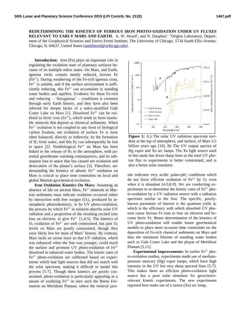
Figure 1: A.) The solar UV radiation spectrum inci-

dent at the top of atmosphere, and surface, of Mars 3.5

billion years ago [10]. B) The UV output spectra of

Hg vapor and Xe arc lamps. The Xe light source used

in this study has fewer sharp lines so the total UV pho-

ton flux to experiments is better constrained, and is

also a better solar simulator.


mailto:[email protected]

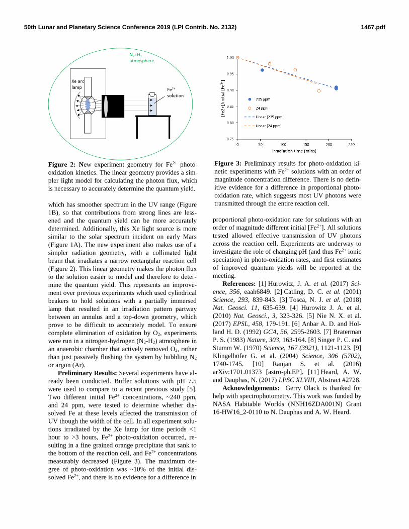
Figure 2: New experiment geometry for Fe2+ photo-

oxidation kinetics. The linear geometry provides a sim-

pler light model for calculating the photon flux, which

is necessary to accurately determine the quantum yield.

which has smoother spectrum in the UV range (Figure

1B), so that contributions from strong lines are less-

ened and the quantum yield can be more accurately

determined. Additionally, this Xe light source is more

similar to the solar spectrum incident on early Mars

(Figure 1A). The new experiment also makes use of a

simpler radiation geometry, with a collimated light

beam that irradiates a narrow rectangular reaction cell

(Figure 2). This linear geometry makes the photon flux

to the solution easier to model and therefore to deter-

mine the quantum yield. This represents an improve-

ment over previous experiments which used cylindrical

beakers to hold solutions with a partially immersed

lamp that resulted in an irradiation pattern partway

between an annulus and a top-down geometry, which

prove to be difficult to accurately model. To ensure

complete elimination of oxidation by O2, experiments

were run in a nitrogen-hydrogen (N2-H2) atmosphere in

an anaerobic chamber that actively removed O2, rather

than just passively flushing the system by bubbling N2

or argon (Ar).

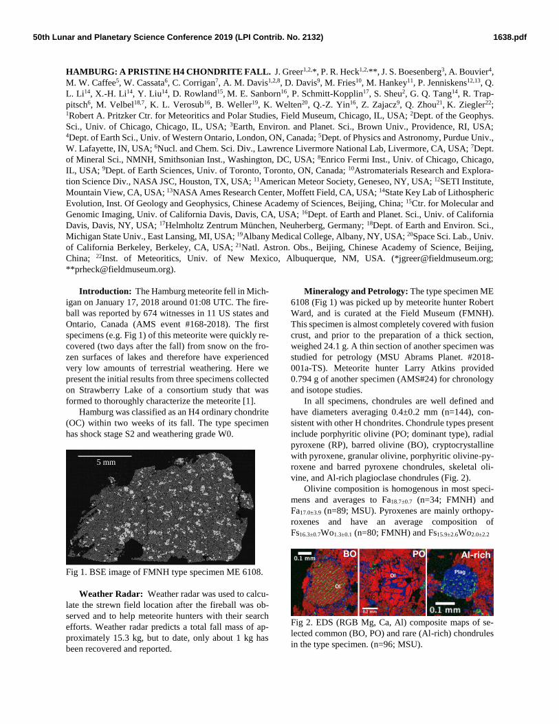
Preliminary Results: Several experiments have al-

ready been conducted. Buffer solutions with pH 7.5

were used to compare to a recent previous study [5].

Two different initial Fe2+ concentrations, ~240 ppm,

and 24 ppm, were tested to determine whether dis-

solved Fe at these levels affected the transmission of

UV though the width of the cell. In all experiment solu-

tions irradiated by the Xe lamp for time periods <1

hour to >3 hours, Fe2+ photo-oxidation occurred, re-

sulting in a fine grained orange precipitate that sank to

the bottom of the reaction cell, and Fe2+ concentrations

measurably decreased (Figure 3). The maximum de-

gree of photo-oxidation was ~10% of the initial dis-

solved Fe2+, and there is no evidence for a difference in

proportional photo-oxidation rate for solutions with an

order of magnitude different initial [Fe2+]. All solutions

tested allowed effective transmission of UV photons

across the reaction cell. Experiments are underway to

investigate the role of changing pH (and thus Fe2+ ionic

speciation) in photo-oxidation rates, and first estimates

of improved quantum yields will be reported at the

meeting.

References: [1] Hurowitz, J. A. et al. (2017) Sci-

ence, 356, eaah6849. [2] Catling, D. C. et al. (2001)

Science, 293, 839-843. [3] Tosca, N. J. et al. (2018)

Nat. Geosci. 11, 635-639. [4] Hurowitz J. A. et al.

(2010) Nat. Geosci., 3, 323-326. [5] Nie N. X. et al.

(2017) EPSL, 458, 179-191. [6] Anbar A. D. and Hol-

land H. D. (1992) GCA, 56, 2595-2603. [7] Braterman

P. S. (1983) Nature, 303, 163-164. [8] Singer P. C. and

Stumm W. (1970) Science, 167 (3921), 1121-1123. [9]

Klingelhöfer G. et al. (2004) Science, 306 (5702),

1740-1745. [10] Ranjan S. et al. (2016)

arXiv:1701.01373 [astro-ph.EP]. [11] Heard, A. W.

and Dauphas, N. (2017) LPSC XLVIII, Abstract #2728.

Acknowledgements: Gerry Olack is thanked for

help with spectrophotometry. This work was funded by

NASA Habitable Worlds (NNH16ZDA001N) Grant

16-HW16_2-0110 to N. Dauphas and A. W. Heard.

Figure 3: Preliminary results for photo-oxidation ki-

netic experiments with Fe2+ solutions with an order of

magnitude concentration difference. There is no defin-

itive evidence for a difference in proportional photo-

oxidation rate, which suggests most UV photons were

transmitted through the entire reaction cell.


HAMBURG: A PRISTINE H4 CHONDRITE FALL. J. Greer1,2,*, P. R. Heck1,2,**, J. S. Boesenberg3, A. Bouvier4,

M. W. Caffee5, W. Cassata6, C. Corrigan7, A. M. Davis1,2,8, D. Davis9, M. Fries10, M. Hankey11, P. Jenniskens12,13, Q.

L. Li14, X.-H. Li14, Y. Liu14, D. Rowland15, M. E. Sanborn16, P. Schmitt-Kopplin17, S. Sheu2, G. Q. Tang14, R. Trap-

pitsch6, M. Velbel18,7, K. L. Verosub16, B. Weller19, K. Welten20, Q.-Z. Yin16, Z. Zajacz9, Q. Zhou21, K. Ziegler22; 1Robert A. Pritzker Ctr. for Meteoritics and Polar Studies, Field Museum, Chicago, IL, USA; 2Dept. of the Geophys.

Sci., Univ. of Chicago, Chicago, IL, USA; 3Earth, Environ. and Planet. Sci., Brown Univ., Providence, RI, USA; 4Dept. of Earth Sci., Univ. of Western Ontario, London, ON, Canada; 5Dept. of Physics and Astronomy, Purdue Univ.,

W. Lafayette, IN, USA; 6Nucl. and Chem. Sci. Div., Lawrence Livermore National Lab, Livermore, CA, USA; 7Dept.

of Mineral Sci., NMNH, Smithsonian Inst., Washington, DC, USA; 8Enrico Fermi Inst., Univ. of Chicago, Chicago,

IL, USA; 9Dept. of Earth Sciences, Univ. of Toronto, Toronto, ON, Canada; 10Astromaterials Research and Explora-

tion Science Div., NASA JSC, Houston, TX, USA; 11American Meteor Society, Geneseo, NY, USA; 12SETI Institute,

Mountain View, CA, USA; 13NASA Ames Research Center, Moffett Field, CA, USA; 14State Key Lab of Lithospheric

Evolution, Inst. Of Geology and Geophysics, Chinese Academy of Sciences, Beijing, China; 15Ctr. for Molecular and

Genomic Imaging, Univ. of California Davis, Davis, CA, USA; 16Dept. of Earth and Planet. Sci., Univ. of California

Davis, Davis, NY, USA; 17Helmholtz Zentrum München, Neuherberg, Germany; 18Dept. of Earth and Environ. Sci.,

Michigan State Univ., East Lansing, MI, USA; 19Albany Medical College, Albany, NY, USA; 20Space Sci. Lab., Univ.

of California Berkeley, Berkeley, CA, USA; 21Natl. Astron. Obs., Beijing, Chinese Academy of Science, Beijing,

China; 22Inst. of Meteoritics, Univ. of New Mexico, Albuquerque, NM, USA. (*[email protected];

**[email protected]).

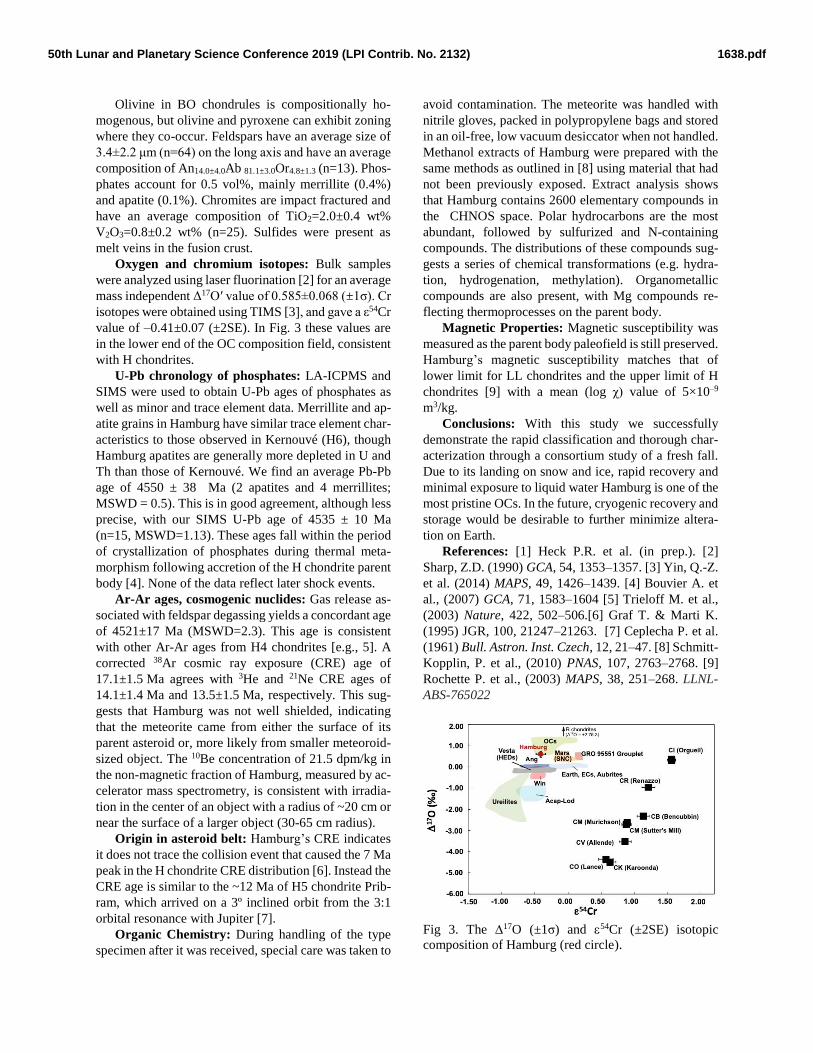
Introduction: The Hamburg meteorite fell in Mich-

igan on January 17, 2018 around 01:08 UTC. The fire-

ball was reported by 674 witnesses in 11 US states and

Ontario, Canada (AMS event #168-2018). The first

specimens (e.g. Fig 1) of this meteorite were quickly re-

covered (two days after the fall) from snow on the fro-

zen surfaces of lakes and therefore have experienced

very low amounts of terrestrial weathering. Here we

present the initial results from three specimens collected

on Strawberry Lake of a consortium study that was

formed to thoroughly characterize the meteorite [1].

Hamburg was classified as an H4 ordinary chondrite

(OC) within two weeks of its fall. The type specimen

has shock stage S2 and weathering grade W0.

Fig 1. BSE image of FMNH type specimen ME 6108.

Weather Radar: Weather radar was used to calcu-

late the strewn field location after the fireball was ob-

served and to help meteorite hunters with their search

efforts. Weather radar predicts a total fall mass of ap-

proximately 15.3 kg, but to date, only about 1 kg has

been recovered and reported.

Mineralogy and Petrology: The type specimen ME

6108 (Fig 1) was picked up by meteorite hunter Robert

Ward, and is curated at the Field Museum (FMNH).

This specimen is almost completely covered with fusion

crust, and prior to the preparation of a thick section,

weighed 24.1 g. A thin section of another specimen was

studied for petrology (MSU Abrams Planet. #2018-

001a-TS). Meteorite hunter Larry Atkins provided

0.794 g of another specimen (AMS#24) for chronology

and isotope studies.

In all specimens, chondrules are well defined and

have diameters averaging 0.4±0.2 mm (n=144), con-

sistent with other H chondrites. Chondrule types present

include porphyritic olivine (PO; dominant type), radial

pyroxene (RP), barred olivine (BO), cryptocrystalline

with pyroxene, granular olivine, porphyritic olivine-py-

roxene and barred pyroxene chondrules, skeletal oli-

vine, and Al-rich plagioclase chondrules (Fig. 2).

Olivine composition is homogenous in most speci-

mens and averages to Fa18.7±0.7 (n=34; FMNH) and

Fa17.0±3.9 (n=89; MSU). Pyroxenes are mainly orthopy-

roxenes and have an average composition of

Fs16.3±0.7Wo1.3±0.1 (n=80; FMNH) and Fs15.9±2.6Wo2.0±2.2

Fig 2. EDS (RGB Mg, Ca, Al) composite maps of se-

lected common (BO, PO) and rare (Al-rich) chondrules

in the type specimen. (n=96; MSU).

5 mm


Olivine in BO chondrules is compositionally ho-

mogenous, but olivine and pyroxene can exhibit zoning

where they co-occur. Feldspars have an average size of

3.4±2.2 μm (n=64) on the long axis and have an average

composition of An14.0±4.0Ab 81.1±3.0Or4.8±1.3 (n=13). Phos-

phates account for 0.5 vol%, mainly merrillite (0.4%)

and apatite (0.1%). Chromites are impact fractured and

have an average composition of TiO2=2.0±0.4 wt%

V2O3=0.8±0.2 wt% (n=25). Sulfides were present as

melt veins in the fusion crust.

Oxygen and chromium isotopes: Bulk samples

were analyzed using laser fluorination [2] for an average

mass independent Δ17O′ value of 0.585±0.068 (±1σ). Cr

isotopes were obtained using TIMS [3], and gave a ε54Cr

value of –0.41±0.07 (±2SE). In Fig. 3 these values are

in the lower end of the OC composition field, consistent

with H chondrites.

U-Pb chronology of phosphates: LA-ICPMS and

SIMS were used to obtain U-Pb ages of phosphates as

well as minor and trace element data. Merrillite and ap-

atite grains in Hamburg have similar trace element char-

acteristics to those observed in Kernouvé (H6), though

Hamburg apatites are generally more depleted in U and

Th than those of Kernouvé. We find an average Pb-Pb

age of 4550 ± 38 Ma (2 apatites and 4 merrillites;

MSWD = 0.5). This is in good agreement, although less

precise, with our SIMS U-Pb age of 4535 ± 10 Ma

(n=15, MSWD=1.13). These ages fall within the period

of crystallization of phosphates during thermal meta-

morphism following accretion of the H chondrite parent

body [4]. None of the data reflect later shock events.

Ar-Ar ages, cosmogenic nuclides: Gas release as-

sociated with feldspar degassing yields a concordant age

of 4521±17 Ma (MSWD=2.3). This age is consistent

with other Ar-Ar ages from H4 chondrites [e.g., 5]. A

corrected 38Ar cosmic ray exposure (CRE) age of

17.1±1.5 Ma agrees with 3He and 21Ne CRE ages of

14.1±1.4 Ma and 13.5±1.5 Ma, respectively. This sug-

gests that Hamburg was not well shielded, indicating

that the meteorite came from either the surface of its

parent asteroid or, more likely from smaller meteoroid-

sized object. The 10Be concentration of 21.5 dpm/kg in

the non-magnetic fraction of Hamburg, measured by ac-

celerator mass spectrometry, is consistent with irradia-

tion in the center of an object with a radius of ~20 cm or

near the surface of a larger object (30-65 cm radius).

Origin in asteroid belt: Hamburg’s CRE indicates

it does not trace the collision event that caused the 7 Ma

peak in the H chondrite CRE distribution [6]. Instead the

CRE age is similar to the ~12 Ma of H5 chondrite Prib-

ram, which arrived on a 3º inclined orbit from the 3:1

orbital resonance with Jupiter [7].

Organic Chemistry: During handling of the type

specimen after it was received, special care was taken to

avoid contamination. The meteorite was handled with

nitrile gloves, packed in polypropylene bags and stored

in an oil-free, low vacuum desiccator when not handled.

Methanol extracts of Hamburg were prepared with the

same methods as outlined in [8] using material that had

not been previously exposed. Extract analysis shows

that Hamburg contains 2600 elementary compounds in

the CHNOS space. Polar hydrocarbons are the most

abundant, followed by sulfurized and N-containing

compounds. The distributions of these compounds sug-

gests a series of chemical transformations (e.g. hydra-

tion, hydrogenation, methylation). Organometallic

compounds are also present, with Mg compounds re-

flecting thermoprocesses on the parent body.

Magnetic Properties: Magnetic susceptibility was

measured as the parent body paleofield is still preserved.

Hamburg’s magnetic susceptibility matches that of

lower limit for LL chondrites and the upper limit of H

chondrites [9] with a mean (log χ) value of 5×10–9

m3/kg.

Conclusions: With this study we successfully

demonstrate the rapid classification and thorough char-

acterization through a consortium study of a fresh fall.

Due to its landing on snow and ice, rapid recovery and

minimal exposure to liquid water Hamburg is one of the

most pristine OCs. In the future, cryogenic recovery and

storage would be desirable to further minimize altera-

tion on Earth.

References: [1] Heck P.R. et al. (in prep.). [2]

Sharp, Z.D. (1990) GCA, 54, 1353–1357. [3] Yin, Q.-Z.

et al. (2014) MAPS, 49, 1426–1439. [4] Bouvier A. et

al., (2007) GCA, 71, 1583–1604 [5] Trieloff M. et al.,

(2003) Nature, 422, 502–506.[6] Graf T. & Marti K.

(1995) JGR, 100, 21247–21263. [7] Ceplecha P. et al.

(1961) Bull. Astron. Inst. Czech, 12, 21–47. [8] Schmitt-

Kopplin, P. et al., (2010) PNAS, 107, 2763–2768. [9]

Rochette P. et al., (2003) MAPS, 38, 251–268. LLNL-

ABS-765022

Fig 3. The 17O (±1σ) and 54Cr (±2SE) isotopic

composition of Hamburg (red circle).


New Insights into Crater Obliteration in the Noachian Highlands of Mars. Samuel J. Holo and Edwin S. Kite University of Chicago, Department of Geophysical Sciences, Chicago, IL, 60637 – [email protected]

Introduction: The Noachian highlands of Mars are

heavily-cratered terrain that, in their geology, record pre-valley-network Mars, the climate of which remains enigmatic (e.g. [1]). The majority of craters on Noa-chian terrain are degraded (e.g. [2]), and several aspects of the Noachian highland landscape can be explained by the interplay of impact cratering and erosion of crater rims by fluvial erosion [3,4]. Further, examination of the latitudinal/elevational trends in crater density and mor-phometric properties has prompted studies on the his-tory of climatic forcing on crater modification and deg-radation (e.g. [2,5]).

The size-frequency distribution (SFD) of craters in the Noachian highlands exhibits a paucity of craters < ~32 km in diameter, relative to extrapolation from isochron fits to larger craters (e.g. [6,7]). This is com-monly interpreted to result from the obliteration of cra-ters by the same surface processes that cause the afore-mentioned crater modification (e.g. [1,2]). However, the observed crater SFD may also be explained by an im-pactor size-frequency distribution that has changed through time, rather than crater obliteration (e.g. [8]).

If caused by crater obliteration, the Noachian crater size-frequency distribution implies ~1 km of terrain-av-eraged erosion [4,6]. This estimate exceeds the implied amount of erosion by valley networks by several orders of magnitude [9]. Thus, the pre-valley-network era may represent the period of Mars’ history with the most flu-vial erosion. In this work, we examine the spatial statis-tics of craters to assess the link between crater degrada-tion and crater obliteration on the Noachian highlands.

Datasets and hypotheses: We used a global geo-logic map of Mars [10] and 2 pixel-per-degree (ppd) gridded MOLA data to generate a 2ppd map of Noa-chian highland units (eNh, mNh and lNh) with their as-sociated elevations (smoothed by nearest-neighbor av-eraging to avoid sampling crater bottoms). Combination of this map with a global database of Martian craters [11] enables us to ask four main questions:

• Is there a signal of a latitude control on crater obliteration?

• Is there a signal of an elevation control on crater obliteration?

• Does the degradation of equatorial craters on Noachian terrain leave a measurable signal of spatial clustering relative to fresh craters?

• Do craters in the 4 km to 32 km range on Noa-chian terrain show a spatial clustering signal more similar to (a) that of the degraded Noa-chian crater population or (b) that of the fresh crater population?

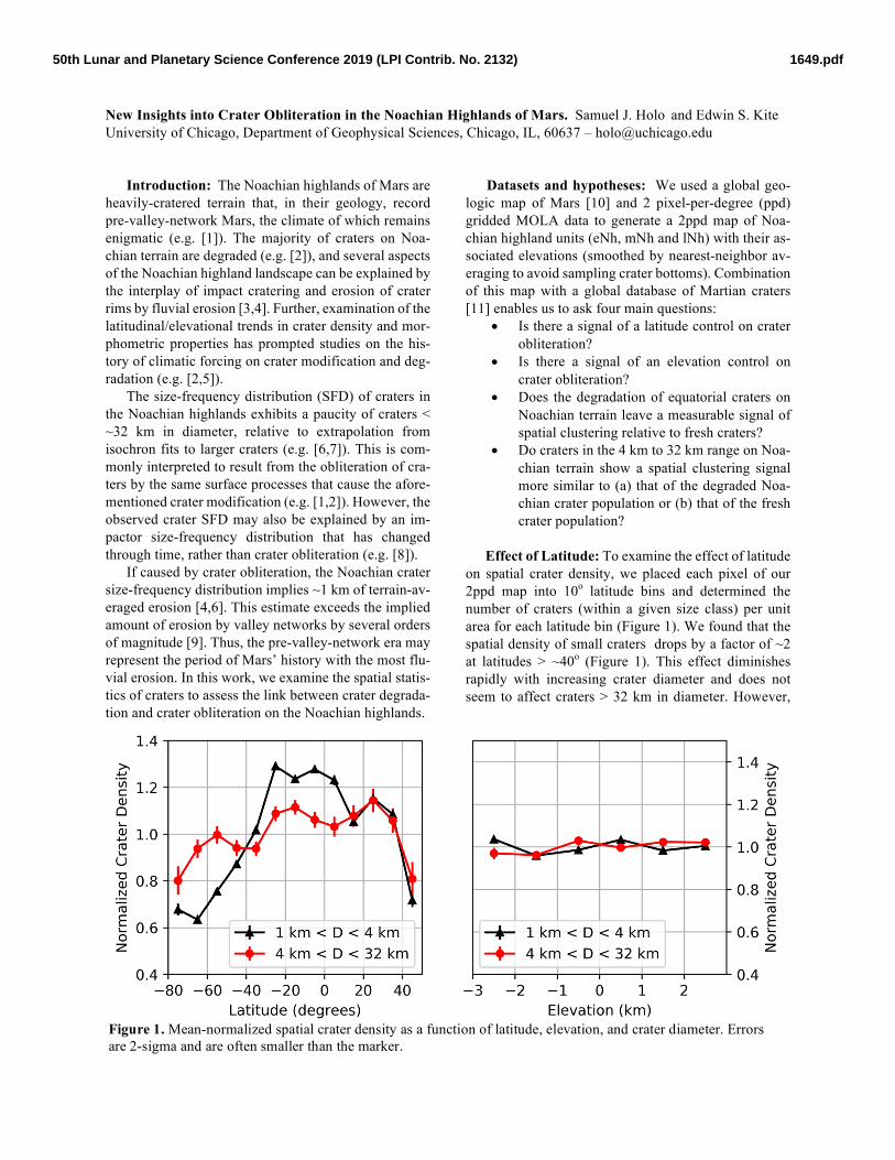
Effect of Latitude: To examine the effect of latitude

on spatial crater density, we placed each pixel of our 2ppd map into 10o latitude bins and determined the number of craters (within a given size class) per unit area for each latitude bin (Figure 1). We found that the spatial density of small craters drops by a factor of ~2 at latitudes > ~40o (Figure 1). This effect diminishes rapidly with increasing crater diameter and does not seem to affect craters > 32 km in diameter. However,

Figure 1. Mean-normalized spatial crater density as a function of latitude, elevation, and crater diameter. Errors are 2-sigma and are often smaller than the marker.


the paucity of small craters that is characteristic of crater SFD’s on Noachian terrains persists at all latitudes.

We interpret our observed signal as Amazonian obliteration of small craters on Noachian terrains in the polar regions. This is consistent with the finding that crater-wall slope degradation (by presumably ice-asso-ciated processes) has continued throughout the Amazo-nian in the polar regions [5]. Our findings suggest that crater degradation can indeed cause crater obliteration but that latitudinally driven processes cannot explain the relative paucity of small craters on Noachian terrain.

Effect of Elevation: Placing our map in 1 km ele-vation bins, we found no significant effect of elevation on crater density in any size bin. This is seemingly at odds with previous observations of degraded crater den-sity [2] and crater-wall slopes [5], which have been used to argue for prolonged crater degradation at low eleva-tions. However, the inferred modification processes need not be responsible for the obliteration of (most of) the craters. The observed degraded Noachian craters could, for example, be the fluvially-modified remnants of a population that was largely obliterated by a second, elevation-insensitive process. Alternatively, the SFD of Mars impactors could have changed since the Noachian.

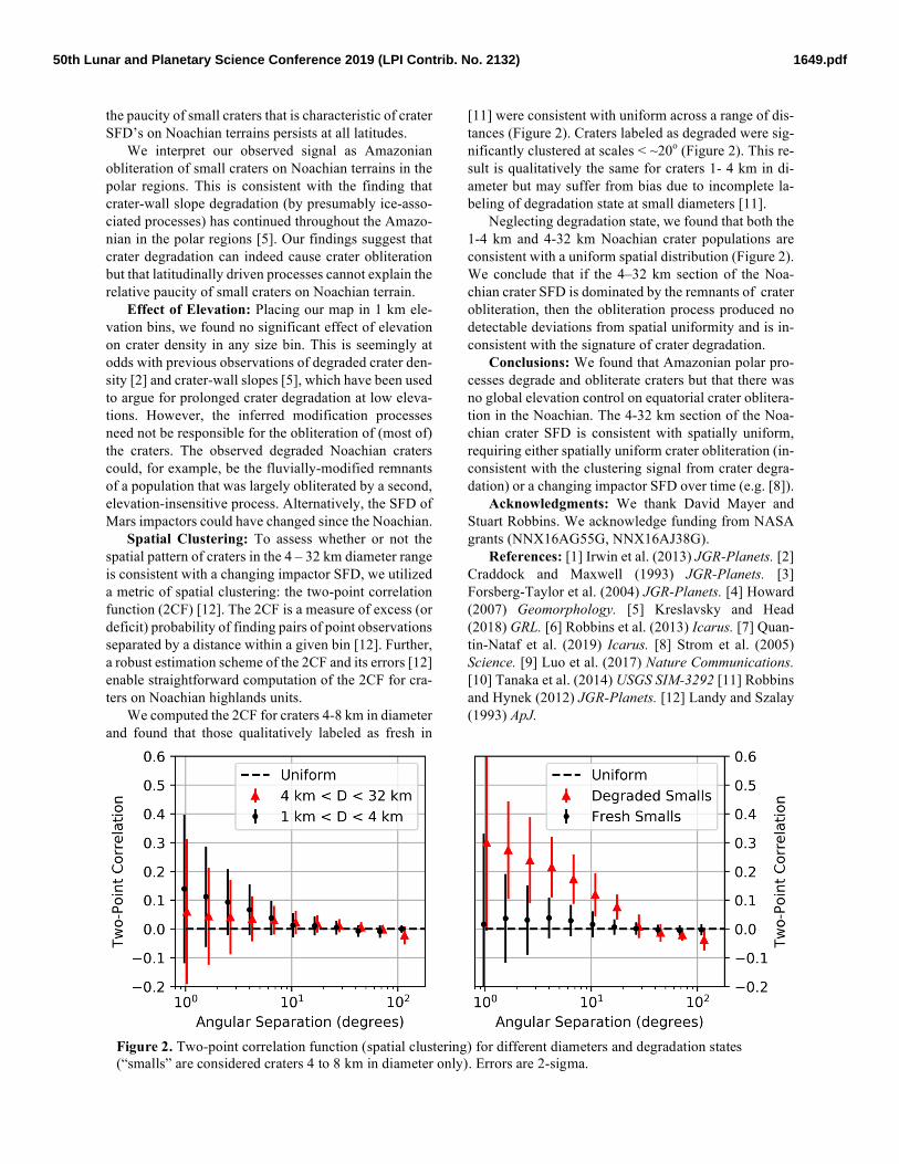
Spatial Clustering: To assess whether or not the spatial pattern of craters in the 4 – 32 km diameter range is consistent with a changing impactor SFD, we utilized a metric of spatial clustering: the two-point correlation function (2CF) [12]. The 2CF is a measure of excess (or deficit) probability of finding pairs of point observations separated by a distance within a given bin [12]. Further, a robust estimation scheme of the 2CF and its errors [12] enable straightforward computation of the 2CF for cra-ters on Noachian highlands units.

We computed the 2CF for craters 4-8 km in diameter and found that those qualitatively labeled as fresh in

[11] were consistent with uniform across a range of dis-tances (Figure 2). Craters labeled as degraded were sig-nificantly clustered at scales < ~20o (Figure 2). This re-sult is qualitatively the same for craters 1- 4 km in di-ameter but may suffer from bias due to incomplete la-beling of degradation state at small diameters [11].

Neglecting degradation state, we found that both the 1-4 km and 4-32 km Noachian crater populations are consistent with a uniform spatial distribution (Figure 2). We conclude that if the 4–32 km section of the Noa-chian crater SFD is dominated by the remnants of crater obliteration, then the obliteration process produced no detectable deviations from spatial uniformity and is in-consistent with the signature of crater degradation.

Conclusions: We found that Amazonian polar pro-cesses degrade and obliterate craters but that there was no global elevation control on equatorial crater oblitera-tion in the Noachian. The 4-32 km section of the Noa-chian crater SFD is consistent with spatially uniform, requiring either spatially uniform crater obliteration (in-consistent with the clustering signal from crater degra-dation) or a changing impactor SFD over time (e.g. [8]).

Acknowledgments: We thank David Mayer and Stuart Robbins. We acknowledge funding from NASA grants (NNX16AG55G, NNX16AJ38G).

References: [1] Irwin et al. (2013) JGR-Planets. [2] Craddock and Maxwell (1993) JGR-Planets. [3] Forsberg-Taylor et al. (2004) JGR-Planets. [4] Howard (2007) Geomorphology. [5] Kreslavsky and Head (2018) GRL. [6] Robbins et al. (2013) Icarus. [7] Quan-tin-Nataf et al. (2019) Icarus. [8] Strom et al. (2005) Science. [9] Luo et al. (2017) Nature Communications. [10] Tanaka et al. (2014) USGS SIM-3292 [11] Robbins and Hynek (2012) JGR-Planets. [12] Landy and Szalay (1993) ApJ.

Figure 2. Two-point correlation function (spatial clustering) for different diameters and degradation states (“smalls” are considered craters 4 to 8 km in diameter only). Errors are 2-sigma.


FORMATION OF LAYERED VS. MIXED ICES IN PROTO-PLANETARY ENVIRONMENTS. M. N. Bar-nett1 and F. J. Ciesla1, 1The University of Chicago, Department of Geophysical Sciences ([email protected])

Introduction: Protoplanetary disks are an initial in-

cubator for complex organic molecules, which can then be incorporated into forming planets and be available for biological processes over time. As more organic molecules are being detected in proto-planetary disks [1-3] it is more important than ever to understand the formation of these organic molecules during the various environments that would exist during planet formation.

Organic molecules can form either in gas phase or grain-surface reactions [4]. In a recent study, CH#CNformation is suggested to be primarily grain-surface reaction based [5] and this may be true for many other organic molecules formed in disks, provided the reactants are able to find one another. As such, under-standing the structures and compositions of the ice man-tles around dust grains is necessary to understanding or-ganic molecule synthesis during planet formation.

Here, we seek to characterize the extent to which mixed ices and layered ices would form in various mo-lecular cloud and protoplanetary disk environments. We focus on studying how simple molecules with a range of volatilities freeze-out and are distributed under a variety of physical environments. We then use this to evaluate which of these environments could support grain-surface reactions or grain-gas reactions which could form organic molecules.

Methods: We use the Astrochem chemical model-ing code [6] to simulate the chemical reactions that would occur at different number densities of hydrogen and temperatures. To start, we use a simplified chemi-cal network selected from the UMIST12 version 2 data-base [7], focusing on thermal desorption off the grain, freeze out, and UV driven photo-desorption. This is so we can isolate only the processes and resulting formula-tion/destruction of ice mantles and their compositions without separate grain surface and gas-grain reactions occurring during model evolution, which we will ex-plore in future studies.

For each set of initial conditions we compare two sets of molecules, N2-CO as examples of species with similar volatilities [8] and H2O-CO as examples of those with very different volatilities. Each species begins en-tirely in the vapor phase at the start of evolution, and the behavior of each molecule in both vapor and ice phase is tracked for 1 million years. We start by exploring the evolution under static conditions holding the gas/grain temperature, optical depth, UV irradiation field (Go), and total abundances of all species and dust grains con-stant throughout evolution.

For each model, during evolution, the ratio of the abundances of each species in the deposited ice is

determined at each time step. We focus on the ratio during the timestep where the greatest increase in the ice layer occurs to determine whether the ice is mixed or layered. The initial ratio of abundances of the species is defined as c& =

()*+,-+).()*+,-+)/

, and the resulting contour

maps of the models display the concentration enrich-ment factor in terms of c&. Ice is considered mixed when the ratio of ice creation of the two species approaches the initial ratio of abundances of the species in the vapor phase. Conversely, ice is considered layered when the ratio of the two species at maximum ice creation is very large compared to the initial vapor abundance ratio, in-dicating that the ice is dominated by one species.

Initial Results and Discussion: For our ice evolu-tion models, we consider a different range of tempera-tures for the N2-CO system vs. the H2O-CO system. For the N2-CO models, we consider a range of temperatures from 14 to 20K, while we consider a temperature range between 8 and 35K for the H2O-CO models. For both sets of models we consider a range of 𝑛1 values between 104 and 105# [cm8#], and we consider a range of UV irradiation values from 0 Go to 100 Go. This range of conditions is meant to simulate all possible conditions seen in molecular clouds and protoplanetary disks.

Figures 1 and 2 show the results of our models for the N2-CO and H2O-CO systems respectively. Not sur-prisingly, the temperature where ices transition from mixed (red) to layered (blue) is a strong function of gas density, and correlates to the freeze-out temperature of the less volatile molecule. In some cases, it is possible that trapping of the less volatile species allows ices to be effectively mixed at conditions where layered ices would form. This would likely be the case at the higher gas densities, where very high deposition rates were possible [9], something we are working to quantify.

These findings show that the formation location or history of ice mantles will play a critical role in deter-mining the structure of the ices and the types of chem-istry that could occur. If mixed ices are needed to allow particular chemical reactions to occur, then these ices must form in conditions where deposition occurs at tem-peratures below the freeze-out temperature of the most volatile species of interest. That is, if interactions be-tween molecules of different volatilities on grain sur-faces are important (such as those that might lead to or-ganic production through UV irradiation [e.g. 10]), then these ices must have formed at very low temperatures. If instead, the ices formed through slow, gradual cooling of a system, the less volatile species would freeze-out first, followed by the freeze-out of the more volatile


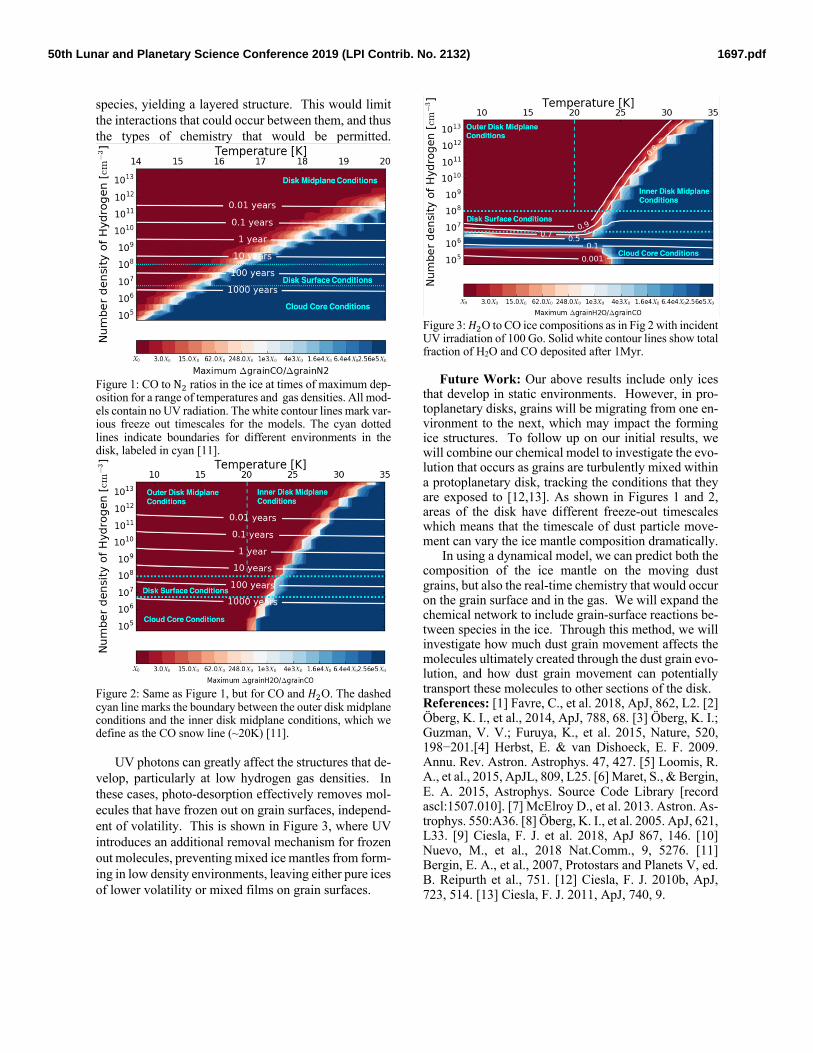
species, yielding a layered structure. This would limit the interactions that could occur between them, and thus the types of chemistry that would be permitted.

Figure 1: CO to N: ratios in the ice at times of maximum dep-osition for a range of temperatures and gas densities. All mod-els contain no UV radiation. The white contour lines mark var-ious freeze out timescales for the models. The cyan dotted lines indicate boundaries for different environments in the disk, labeled in cyan [11].

Figure 2: Same as Figure 1, but for CO and 𝐻:O. The dashed cyan line marks the boundary between the outer disk midplane conditions and the inner disk midplane conditions, which we define as the CO snow line (~20K) [11].

UV photons can greatly affect the structures that de-velop, particularly at low hydrogen gas densities. In these cases, photo-desorption effectively removes mol-ecules that have frozen out on grain surfaces, independ-ent of volatility. This is shown in Figure 3, where UV introduces an additional removal mechanism for frozen out molecules, preventing mixed ice mantles from form-ing in low density environments, leaving either pure ices of lower volatility or mixed films on grain surfaces.

Figure 3: 𝐻:O to CO ice compositions as in Fig 2 with incident UV irradiation of 100 Go. Solid white contour lines show total fraction of H2O and CO deposited after 1Myr.

Future Work: Our above results include only ices that develop in static environments. However, in pro-toplanetary disks, grains will be migrating from one en-vironment to the next, which may impact the forming ice structures. To follow up on our initial results, we will combine our chemical model to investigate the evo-lution that occurs as grains are turbulently mixed within a protoplanetary disk, tracking the conditions that they are exposed to [12,13]. As shown in Figures 1 and 2, areas of the disk have different freeze-out timescales which means that the timescale of dust particle move-ment can vary the ice mantle composition dramatically.

In using a dynamical model, we can predict both the composition of the ice mantle on the moving dust grains, but also the real-time chemistry that would occur on the grain surface and in the gas. We will expand the chemical network to include grain-surface reactions be-tween species in the ice. Through this method, we will investigate how much dust grain movement affects the molecules ultimately created through the dust grain evo-lution, and how dust grain movement can potentially transport these molecules to other sections of the disk. References: [1] Favre, C., et al. 2018, ApJ, 862, L2. [2] Öberg, K. I., et al., 2014, ApJ, 788, 68. [3] Öberg, K. I.; Guzman, V. V.; Furuya, K., et al. 2015, Nature, 520, 198−201.[4] Herbst, E. & van Dishoeck, E. F. 2009. Annu. Rev. Astron. Astrophys. 47, 427. [5] Loomis, R. A., et al., 2015, ApJL, 809, L25. [6] Maret, S., & Bergin, E. A. 2015, Astrophys. Source Code Library [record ascl:1507.010]. [7] McElroy D., et al. 2013. Astron. As-trophys. 550:A36. [8] Öberg, K. I., et al. 2005. ApJ, 621, L33. [9] Ciesla, F. J. et al. 2018, ApJ 867, 146. [10] Nuevo, M., et al., 2018 Nat.Comm., 9, 5276. [11] Bergin, E. A., et al., 2007, Protostars and Planets V, ed. B. Reipurth et al., 751. [12] Ciesla, F. J. 2010b, ApJ, 723, 514. [13] Ciesla, F. J. 2011, ApJ, 740, 9.


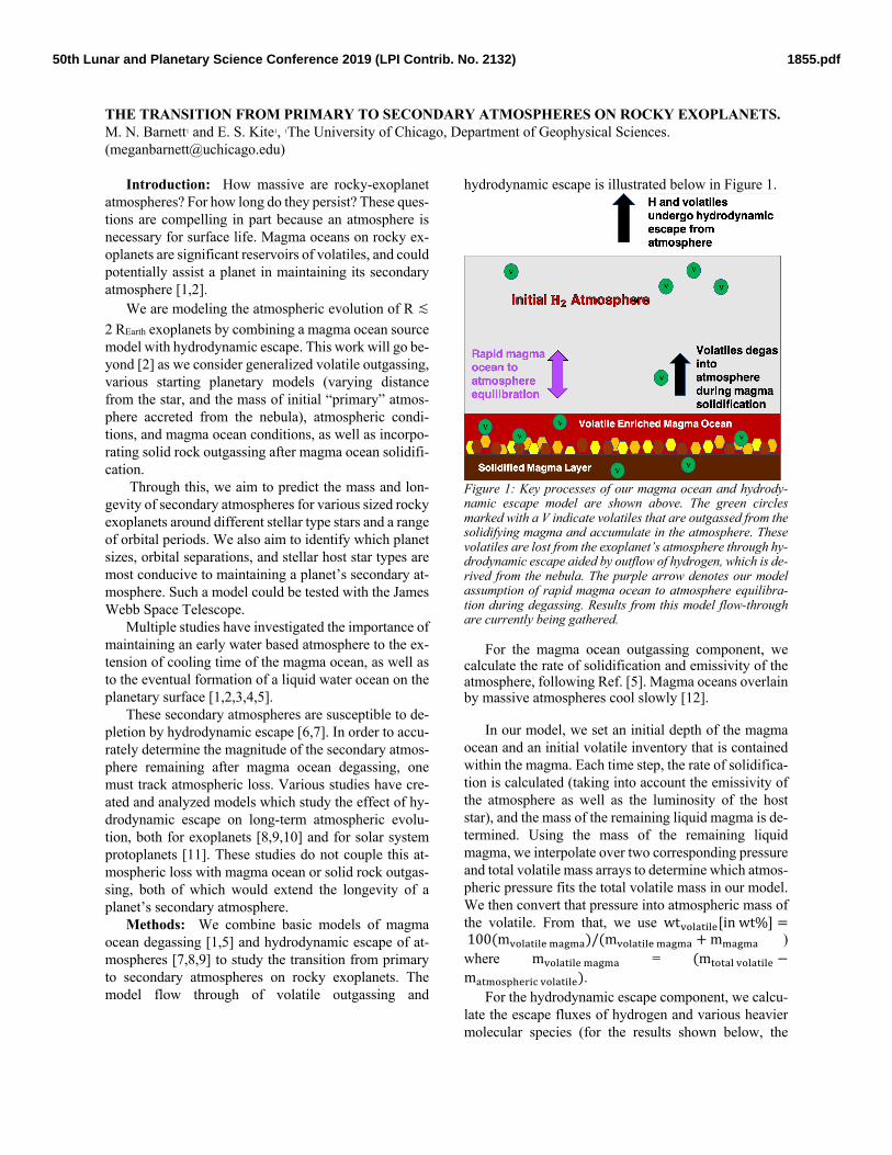
THE TRANSITION FROM PRIMARY TO SECONDARY ATMOSPHERES ON ROCKY EXOPLANETS. M. N. Barnett1 and E. S. Kite1, 1The University of Chicago, Department of Geophysical Sciences. ([email protected])

Introduction: How massive are rocky-exoplanet

atmospheres? For how long do they persist? These ques-tions are compelling in part because an atmosphere is necessary for surface life. Magma oceans on rocky ex-oplanets are significant reservoirs of volatiles, and could potentially assist a planet in maintaining its secondary atmosphere [1,2].

We are modeling the atmospheric evolution of R ≲ 2 REarth exoplanets by combining a magma ocean source model with hydrodynamic escape. This work will go be-yond [2] as we consider generalized volatile outgassing, various starting planetary models (varying distance from the star, and the mass of initial “primary” atmos-phere accreted from the nebula), atmospheric condi-tions, and magma ocean conditions, as well as incorpo-rating solid rock outgassing after magma ocean solidifi-cation.

Through this, we aim to predict the mass and lon-gevity of secondary atmospheres for various sized rocky exoplanets around different stellar type stars and a range of orbital periods. We also aim to identify which planet sizes, orbital separations, and stellar host star types are most conducive to maintaining a planet’s secondary at-mosphere. Such a model could be tested with the James Webb Space Telescope.

Multiple studies have investigated the importance of maintaining an early water based atmosphere to the ex-tension of cooling time of the magma ocean, as well as to the eventual formation of a liquid water ocean on the planetary surface [1,2,3,4,5].

These secondary atmospheres are susceptible to de-pletion by hydrodynamic escape [6,7]. In order to accu-rately determine the magnitude of the secondary atmos-phere remaining after magma ocean degassing, one must track atmospheric loss. Various studies have cre-ated and analyzed models which study the effect of hy-drodynamic escape on long-term atmospheric evolu-tion, both for exoplanets [8,9,10] and for solar system protoplanets [11]. These studies do not couple this at-mospheric loss with magma ocean or solid rock outgas-sing, both of which would extend the longevity of a planet’s secondary atmosphere.

Methods: We combine basic models of magma ocean degassing [1,5] and hydrodynamic escape of at-mospheres [7,8,9] to study the transition from primary to secondary atmospheres on rocky exoplanets. The model flow through of volatile outgassing and

hydrodynamic escape is illustrated below in Figure 1.

Figure 1: Key processes of our magma ocean and hydrody-namic escape model are shown above. The green circles marked with a V indicate volatiles that are outgassed from the solidifying magma and accumulate in the atmosphere. These volatiles are lost from the exoplanet’s atmosphere through hy-drodynamic escape aided by outflow of hydrogen, which is de-rived from the nebula. The purple arrow denotes our model assumption of rapid magma ocean to atmosphere equilibra-tion during degassing. Results from this model flow-through are currently being gathered.

For the magma ocean outgassing component, we calculate the rate of solidification and emissivity of the atmosphere, following Ref. [5]. Magma oceans overlain by massive atmospheres cool slowly [12].

In our model, we set an initial depth of the magma ocean and an initial volatile inventory that is contained within the magma. Each time step, the rate of solidifica-tion is calculated (taking into account the emissivity of the atmosphere as well as the luminosity of the host star), and the mass of the remaining liquid magma is de-termined. Using the mass of the remaining liquid magma, we interpolate over two corresponding pressure and total volatile mass arrays to determine which atmos-pheric pressure fits the total volatile mass in our model. We then convert that pressure into atmospheric mass of the volatile. From that, we use wt#$%&'(%)[inwt%] =100(m#$%&'(%)5&65&)/(m#$%&'(%)5&65& + m5&65& ) where m#$%&'(%)5&65& = (m'$'&%#$%&'(%) −m&'5$;<=)>(?#$%&'(%)).

For the hydrodynamic escape component, we calcu-late the escape fluxes of hydrogen and various heavier molecular species (for the results shown below, the


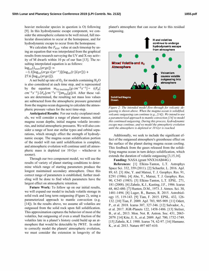
heavier molecular species in question is O) following [9]. In this hydrodynamic escape component, we con-sider the atmospheric column to be well mixed, full mo-lecular dissociation to occur at the homopause, and for hydrodynamic escape to occur from the homopause.

We calculate the 𝐹ABC value at each timestep by us-ing an equation that was interpolated from the graphical results from research surveying the UV and X-ray activ-ity of M dwarfs within 10 pc of our Sun [13]. The re-sulting interpolated equation is as follows: logGH(𝐿ABC[𝑒𝑟𝑔𝑠]) =−1.1[logGH(𝑒𝑟𝑔𝑠𝐺𝑦𝑟QG)](logGH(𝑡[𝐺𝑦𝑟])) +27.6[logGH(𝑒𝑟𝑔𝑠)]).

A net build up rate of OW for models containing HWO is also considered at each time step, and is represented by the equation 𝑚ZW[\]^_\`[𝑔𝑐𝑚QW𝑠QG]= ((𝐹b[ 𝑐𝑚QW𝑠QG]-2𝐹Z[𝑐𝑚QW𝑠QG])𝑚ZW[𝑔])/4. After these val-ues are determined, the resulting net mass loss values are subtracted from the atmospheric pressure generated from the magma ocean degassing to calculate the atmos-pheric pressure values for the next time-step.

Anticipated Results: For our rocky exoplanet mod-els, we will consider a range of planet masses, initial magma ocean depths, initial magma volatile invento-ries, and initial atmospheric pressures. We will also con-sider a range of host star stellar types and orbital sepa-rations, which strongly effect the strength of hydrody-namic escape. The magma ocean solidification portion of the model will run until solidification is complete, and atmospheric evolution will continue until all atmos-pheric mass is depleted (or 10 Gyr – whichever is sooner).

Through our two component model, we will use the results of variety of planet starting conditions to deter-mine which range of starting parameters produce the longest maintained secondary atmosphere. Once this correct range of parameters is established, further mod-eling will be done to find which parameters have the largest effect on atmospheric retention.

Future Work: To follow up on our initial results, we will expand our model to include volatile storage in solid rock and long term outgassing (Figure 2), using a parameterized approach to mantle convection (e.g. [14]). In the results above, we assume all volatiles are outgassed from the solid rock upon full solidification. This approximation captures the behavior of most of the volatiles, but outgassing of even a small fraction of the volatiles late in a planet’s history could build up an at-mosphere that would be detectable by JWST. In order to correctly model the planets' atmospheric evolution, we must consider the extension in longevity of the

planet's atmosphere that can occur due to this residual outgassing.

Figure 2: The intended model flow-through for volcanic de-gassing is shown above. When the magma ocean is solidified, volcanic outgassing can continue (e.g., [14]). We intend to use a parameterized approach to mantle convection [14] to model this continued outgassing. During this process, hydrodynamic escape may continue, and we model the atmospheric evolution until the atmosphere is depleted or 10 Gyr is reached.

Additionally, we seek to include the significant ef-fect of the outgassed atmosphere's greenhouse effect on the surface of the planet during magma ocean cooling. This feedback from the gases released from the solidi-fying magma ocean in turn delays solidification, which extends the duration of volatile outgassing [3,15,16].

Funding: NASA (grant NNX16AB44G.) References: [1] Elkins-Tanton, L.T. Astrophys

Space Sci. 332, 359 (2011). [2] Schaefer, L. 2016. ApJ. 89, 63. [3] Abe, Y. and Matsui, T. J. Geophys. Res. 91, E291 (1986). [4] Abe, Y., Matsui, T. J. Geophys. Res. 90, C545 (1985). [5] Elkins-Tanton, L.T. EPSL. 271, 181 (2008). [6] Zahnle, K.J., Kasting, J.F., 1986. Icarus 68, 462-480. [7] Hunten, D.M., 1973. J. Atmos. Sci. 30, 1481-1494. [8] Luger, R., Barnes, R. 2015. Astrobiol-ogy 15, 119-143. [9] Tian, F. 2015. EPSL. 432, 126-132. [10] Tian, F. 2009. ApJ. 703, 905-909. [11] Odert, P., et al. 2018. Icarus 307, 327-346. [12] Salvador, A., et al. 2017. JGR-Planets 122, 1458-1486. [13] Stelzer, B., et al., 2013. Mon. Not. R. Astron. Soc. 431, 2063-2079. [14] Kite, E. S., et al. 2009. ApJ. 700, 1732-1749. [15] Zahnle, K.J. 1988. Icarus 74, 62-97. [16] Hamano. K., et al. 2013. Nature 497 607-610.


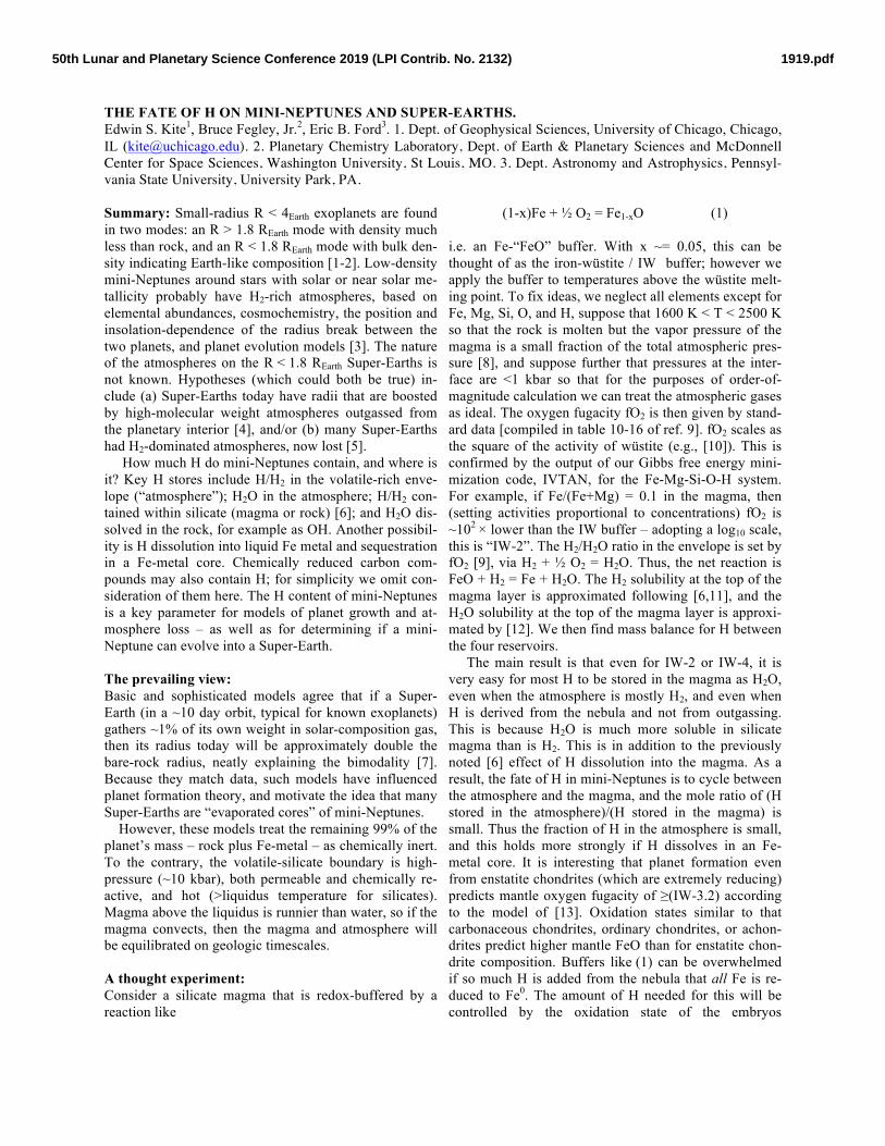
THE FATE OF H ON MINI-NEPTUNES AND SUPER-EARTHS. Edwin S. Kite1, Bruce Fegley, Jr.2, Eric B. Ford3. 1. Dept. of Geophysical Sciences, University of Chicago, Chicago, IL ([email protected]). 2. Planetary Chemistry Laboratory, Dept. of Earth & Planetary Sciences and McDonnell Center for Space Sciences, Washington University, St Louis, MO. 3. Dept. Astronomy and Astrophysics, Pennsyl-vania State University, University Park, PA. Summary: Small-radius R < 4Earth exoplanets are found in two modes: an R > 1.8 REarth mode with density much less than rock, and an R < 1.8 REarth mode with bulk den-sity indicating Earth-like composition [1-2]. Low-density mini-Neptunes around stars with solar or near solar me-tallicity probably have H2-rich atmospheres, based on elemental abundances, cosmochemistry, the position and insolation-dependence of the radius break between the two planets, and planet evolution models [3]. The nature of the atmospheres on the R < 1.8 REarth Super-Earths is not known. Hypotheses (which could both be true) in-clude (a) Super-Earths today have radii that are boosted by high-molecular weight atmospheres outgassed from the planetary interior [4], and/or (b) many Super-Earths had H2-dominated atmospheres, now lost [5]. How much H do mini-Neptunes contain, and where is it? Key H stores include H/H2 in the volatile-rich enve-lope (“atmosphere”); H2O in the atmosphere; H/H2 con-tained within silicate (magma or rock) [6]; and H2O dis-solved in the rock, for example as OH. Another possibil-ity is H dissolution into liquid Fe metal and sequestration in a Fe-metal core. Chemically reduced carbon com-pounds may also contain H; for simplicity we omit con-sideration of them here. The H content of mini-Neptunes is a key parameter for models of planet growth and at-mosphere loss – as well as for determining if a mini-Neptune can evolve into a Super-Earth. The prevailing view: Basic and sophisticated models agree that if a Super-Earth (in a ~10 day orbit, typical for known exoplanets) gathers ~1% of its own weight in solar-composition gas, then its radius today will be approximately double the bare-rock radius, neatly explaining the bimodality [7]. Because they match data, such models have influenced planet formation theory, and motivate the idea that many Super-Earths are “evaporated cores” of mini-Neptunes. However, these models treat the remaining 99% of the planet’s mass – rock plus Fe-metal – as chemically inert. To the contrary, the volatile-silicate boundary is high-pressure (~10 kbar), both permeable and chemically re-active, and hot (>liquidus temperature for silicates). Magma above the liquidus is runnier than water, so if the magma convects, then the magma and atmosphere will be equilibrated on geologic timescales. A thought experiment: Consider a silicate magma that is redox-buffered by a reaction like

(1-x)Fe + ½ O2 = Fe1-xO (1) i.e. an Fe-“FeO” buffer. With x ~= 0.05, this can be thought of as the iron-wüstite / IW buffer; however we apply the buffer to temperatures above the wüstite melt-ing point. To fix ideas, we neglect all elements except for Fe, Mg, Si, O, and H, suppose that 1600 K < T < 2500 K so that the rock is molten but the vapor pressure of the magma is a small fraction of the total atmospheric pres-sure [8], and suppose further that pressures at the inter-face are <1 kbar so that for the purposes of order-of-magnitude calculation we can treat the atmospheric gases as ideal. The oxygen fugacity fO2 is then given by stand-ard data [compiled in table 10-16 of ref. 9]. fO2 scales as the square of the activity of wüstite (e.g., [10]). This is confirmed by the output of our Gibbs free energy mini-mization code, IVTAN, for the Fe-Mg-Si-O-H system. For example, if Fe/(Fe+Mg) = 0.1 in the magma, then (setting activities proportional to concentrations) fO2 is ~102 × lower than the IW buffer – adopting a log10 scale, this is “IW-2”. The H2/H2O ratio in the envelope is set by fO2 [9], via H2 + ½ O2 = H2O. Thus, the net reaction is FeO + H2 = Fe + H2O. The H2 solubility at the top of the magma layer is approximated following [6,11], and the H2O solubility at the top of the magma layer is approxi-mated by [12]. We then find mass balance for H between the four reservoirs. The main result is that even for IW-2 or IW-4, it is very easy for most H to be stored in the magma as H2O, even when the atmosphere is mostly H2, and even when H is derived from the nebula and not from outgassing. This is because H2O is much more soluble in silicate magma than is H2. This is in addition to the previously noted [6] effect of H dissolution into the magma. As a result, the fate of H in mini-Neptunes is to cycle between the atmosphere and the magma, and the mole ratio of (H stored in the atmosphere)/(H stored in the magma) is small. Thus the fraction of H in the atmosphere is small, and this holds more strongly if H dissolves in an Fe-metal core. It is interesting that planet formation even from enstatite chondrites (which are extremely reducing) predicts mantle oxygen fugacity of ≥(IW-3.2) according to the model of [13]. Oxidation states similar to that carbonaceous chondrites, ordinary chondrites, or achon-drites predict higher mantle FeO than for enstatite chon-drite composition. Buffers like (1) can be overwhelmed if so much H is added from the nebula that all Fe is re-duced to Fe0. The amount of H needed for this will be controlled by the oxidation state of the embryos


(±pebbles) that collide to form the rock+metal cores, as reflected by silicate FeO content. Discussion. On Earth, most reducing power is sequestered at the cen-ter of the planet as an Fe core. But this is increasingly difficult at the T > 4000K temperatures predicted by mini-Neptune evolution models [14], because metal and silicate are increasingly miscible at T > 4000K [15]. Open questions include: (1) Can the inflated radii of mini-Neptunes be explained by H2O delivery to Fe-metal-rich worlds, and subsequent outgassing of H2, without accretion of nebular H2? This has been shown to be (just) stochiometrically possible [16]. However, add-ing the requirement of chemical equilibrium, and consid-ering C delivery, strongly supports the prevailing view that the mini-Neptune densities and radii require accre-tion of nebular gas. (2) What is the maximum exoplanet radius boost for outgassing? This is important for inter-preting the densities of short-period Super-Earths detect-ed by Kepler and TESS, and for constraining the origin of the volatile envelopes of small-radius exoplanets clos-er to the habitable zone. At the conference, we will present our answers to these open questions, and discussion of the fate of H on mini-Neptunes and Super-Earths with magma-ocean surfaces at higher T and P. Funding: NASA (grant NNX16AB44G.) References: [1] Fulton, B., et al., 2017, Astron. J. 154, article id 109. [2] Rogers, L., 2015, Astrophys. J. 801, article id. 41. [3] van Eylen, V., et al., 2018, MNRAS 479, 4786-. [4] Tian, F., 2009, Astrophys. J. [5] Owen J. E., Wu Y., 2017, ApJ , 847, 29. [6] Chachan, Y., & Ste-venson, D.J., 2018, Astrophys. J. 854, article id. 21. [7] Lopez, E., & Fortney, J.J., 2014, Astrophys. J., arti-cle id. 1. [8] Fegley, B., et al., 2016, Astrophys. J., arti-cle id. 103. [9] Fegley, B., Practical Chemical Thermo-dynamics for Geoscientists, Elsevier, 2013. [10] Frost, D.J., et al., 2008, Philos. Trans. R. Soc., Math. Phys. Eng. Sci. 366, 4315–4337 [11] Hirschmann, M.M., et al., 2012, EPSL 345, 38–48.. [12] Zahnle, K.J., et al., 1988, Icarus 74, 62-97. [13] Javoy, M., et al., 2010, EPSL 293, 259-268. [14] Howe, A. & Burrows, A., 2015, Astrophys. J. 808, article id. 150. [15] Wahl, S.M., & Militzer, B.. EPSL 410, 25-33. [16] Rogers, L. A., & Seager, S., 2010, Astrophys. J. 716, 1208-1216.


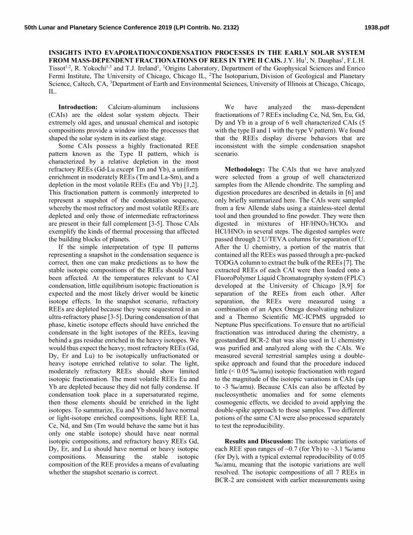
INSIGHTS INTO EVAPORATION/CONDENSATION PROCESSES IN THE EARLY SOLAR SYSTEM FROM MASS-DEPENDENT FRACTIONATIONS OF REES IN TYPE II CAIS. J.Y. Hu1, N. Dauphas1, F.L.H. Tissot1,2, R. Yokochi1,3 and T.J. Ireland1, 1Origins Laboratory, Department of the Geophysical Sciences and Enrico Fermi Institute, The University of Chicago, Chicago IL, 2The Isotoparium, Division of Geological and Planetary Science, Caltech, CA, 3Department of Earth and Environmental Sciences, University of Illinois at Chicago, Chicago, IL.

Introduction: Calcium-aluminum inclusions (CAIs) are the oldest solar system objects. Their extremely old ages, and unusual chemical and isotopic compositions provide a window into the processes that shaped the solar system in its earliest stage.

Some CAIs possess a highly fractionated REE pattern known as the Type II pattern, which is characterized by a relative depletion in the most refractory REEs (Gd-Lu except Tm and Yb), a uniform enrichment in moderately REEs (Tm and La-Sm), and a depletion in the most volatile REEs (Eu and Yb) [1,2]. This fractionation pattern is commonly interpreted to represent a snapshot of the condensation sequence, whereby the most refractory and most volatile REEs are depleted and only those of intermediate refractoriness are present in their full complement [3-5]. Those CAIs exemplify the kinds of thermal processing that affected the building blocks of planets.

If the simple interpretation of type II patterns representing a snapshot in the condensation sequence is correct, then one can make predictions as to how the stable isotopic compositions of the REEs should have been affected. At the temperatures relevant to CAI condensation, little equilibrium isotopic fractionation is expected and the most likely driver would be kinetic isotope effects. In the snapshot scenario, refractory REEs are depleted because they were sequestered in an ultra-refractory phase [3-5]. During condensation of that phase, kinetic isotope effects should have enriched the condensate in the light isotopes of the REEs, leaving behind a gas residue enriched in the heavy isotopes. We would thus expect the heavy, most refractory REEs (Gd, Dy, Er and Lu) to be isotopically unfractionated or heavy isotope enriched relative to solar. The light, moderately refractory REEs should show limited isotopic fractionation. The most volatile REEs Eu and Yb are depleted because they did not fully condense. If condensation took place in a supersaturated regime, then those elements should be enriched in the light isotopes. To summarize, Eu and Yb should have normal or light-isotope enriched compositions, light REE La, Ce, Nd, and Sm (Tm would behave the same but it has only one stable isotope) should have near normal isotopic compositions, and refractory heavy REEs Gd, Dy, Er, and Lu should have normal or heavy isotopic compositions. Measuring the stable isotopic composition of the REE provides a means of evaluating whether the snapshot scenario is correct.

We have analyzed the mass-dependent fractionations of 7 REEs including Ce, Nd, Sm, Eu, Gd, Dy and Yb in a group of 6 well characterized CAIs (5 with the type II and 1 with the type V pattern). We found that the REEs display diverse behaviors that are inconsistent with the simple condensation snapshot scenario.

Methodology: The CAIs that we have analyzed

were selected from a group of well characterized samples from the Allende chondrite. The sampling and digestion procedures are described in details in [6] and only briefly summarized here. The CAIs were sampled from a few Allende slabs using a stainless-steel dental tool and then grounded to fine powder. They were then digested in mixtures of HF/HNO3/HClO4 and HCl/HNO3 in several steps. The digested samples were passed through 2 U/TEVA columns for separation of U. After the U chemistry, a portion of the matrix that contained all the REEs was passed through a pre-packed TODGA column to extract the bulk of the REEs [7]. The extracted REEs of each CAI were then loaded onto a FluoroPolymer Liquid Chromatography system (FPLC) developed at the University of Chicago [8,9] for separation of the REEs from each other. After separation, the REEs were measured using a combination of an Apex Omega desolvating nebulizer and a Thermo Scientific MC-ICPMS upgraded to Neptune Plus specifications. To ensure that no artificial fractionation was introduced during the chemistry, a geostandard BCR-2 that was also used in U chemistry was purified and analyzed along with the CAIs. We measured several terrestrial samples using a double-spike approach and found that the procedure induced little (< 0.05 ‰/amu) isotopic fractionation with regard to the magnitude of the isotopic variations in CAIs (up to -3 ‰/amu). Because CAIs can also be affected by nucleosynthetic anomalies and for some elements cosmogenic effects, we decided to avoid applying the double-spike approach to those samples. Two different potions of the same CAI were also processed separately to test the reproducibility.

Results and Discussion: The isotopic variations of each REE span ranges of ~0.7 (for Yb) to ~3.1 ‰/amu (for Dy), with a typical external reproducibility of 0.05 ‰/amu, meaning that the isotopic variations are well resolved. The isotopic compositions of all 7 REEs in BCR-2 are consistent with earlier measurements using


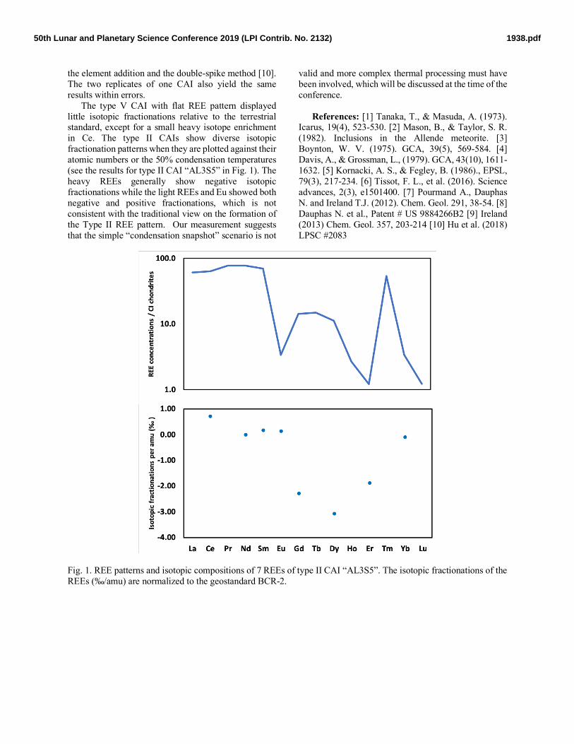
the element addition and the double-spike method [10]. The two replicates of one CAI also yield the same results within errors.

The type V CAI with flat REE pattern displayed little isotopic fractionations relative to the terrestrial standard, except for a small heavy isotope enrichment in Ce. The type II CAIs show diverse isotopic fractionation patterns when they are plotted against their atomic numbers or the 50% condensation temperatures (see the results for type II CAI “AL3S5” in Fig. 1). The heavy REEs generally show negative isotopic fractionations while the light REEs and Eu showed both negative and positive fractionations, which is not consistent with the traditional view on the formation of the Type II REE pattern. Our measurement suggests that the simple “condensation snapshot” scenario is not

valid and more complex thermal processing must have been involved, which will be discussed at the time of the conference.

References: [1] Tanaka, T., & Masuda, A. (1973).

Icarus, 19(4), 523-530. [2] Mason, B., & Taylor, S. R. (1982). Inclusions in the Allende meteorite. [3] Boynton, W. V. (1975). GCA, 39(5), 569-584. [4] Davis, A., & Grossman, L., (1979). GCA, 43(10), 1611-1632. [5] Kornacki, A. S., & Fegley, B. (1986)., EPSL, 79(3), 217-234. [6] Tissot, F. L., et al. (2016). Science advances, 2(3), e1501400. [7] Pourmand A., Dauphas N. and Ireland T.J. (2012). Chem. Geol. 291, 38-54. [8] Dauphas N. et al., Patent # US 9884266B2 [9] Ireland (2013) Chem. Geol. 357, 203-214 [10] Hu et al. (2018) LPSC #2083

Fig. 1. REE patterns and isotopic compositions of 7 REEs of type II CAI “AL3S5”. The isotopic fractionations of the REEs (‰/amu) are normalized to the geostandard BCR-2.


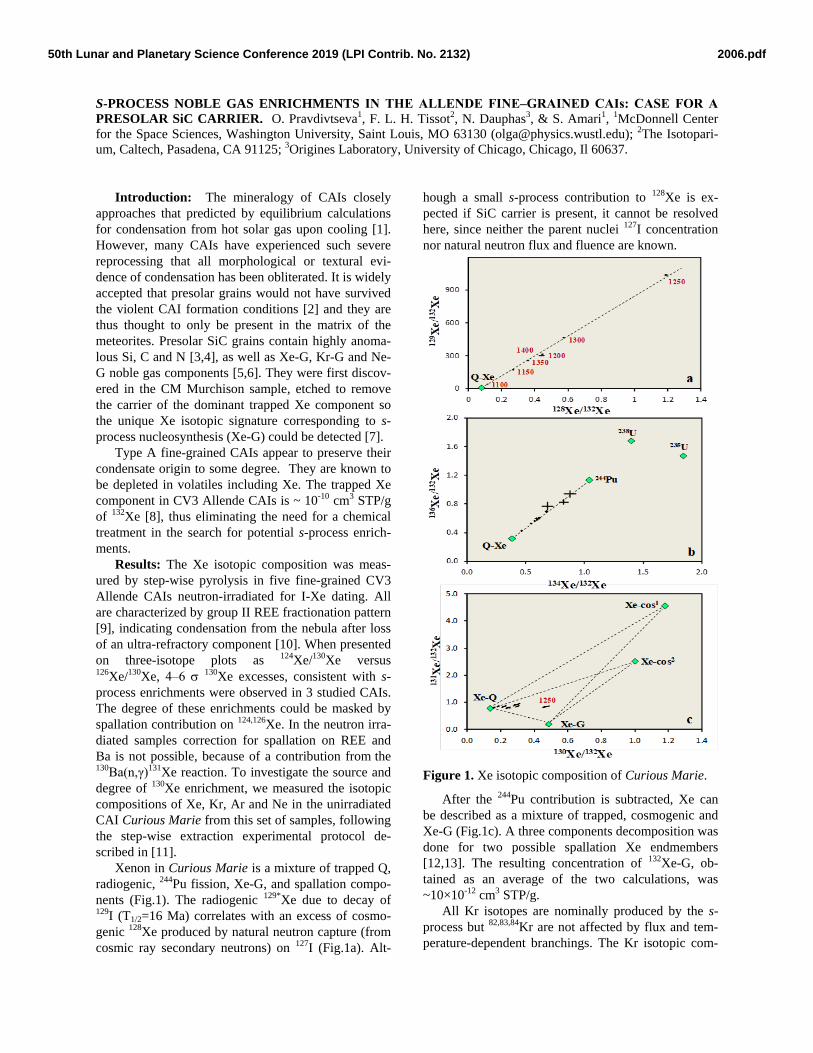
S-PROCESS NOBLE GAS ENRICHMENTS IN THE ALLENDE FINE‒GRAINED CAIs: CASE FOR A

PRESOLAR SiC CARRIER. O. Pravdivtseva1, F. L. H. Tissot2, N. Dauphas3, & S. Amari1, 1McDonnell Center

for the Space Sciences, Washington University, Saint Louis, MO 63130 ([email protected]); 2The Isotopari-

um, Caltech, Pasadena, CA 91125; 3Origines Laboratory, University of Chicago, Chicago, Il 60637.

Introduction: The mineralogy of CAIs closely

approaches that predicted by equilibrium calculations

for condensation from hot solar gas upon cooling [1].

However, many CAIs have experienced such severe

reprocessing that all morphological or textural evi-

dence of condensation has been obliterated. It is widely

accepted that presolar grains would not have survived

the violent CAI formation conditions [2] and they are

thus thought to only be present in the matrix of the

meteorites. Presolar SiC grains contain highly anoma-

lous Si, C and N [3,4], as well as Xe-G, Kr-G and Ne-

G noble gas components [5,6]. They were first discov-

ered in the CM Murchison sample, etched to remove

the carrier of the dominant trapped Xe component so

the unique Xe isotopic signature corresponding to s-

process nucleosynthesis (Xe-G) could be detected [7].

Type A fine-grained CAIs appear to preserve their

condensate origin to some degree. They are known to

be depleted in volatiles including Xe. The trapped Xe

component in CV3 Allende CAIs is ~ 10-10 cm3 STP/g

of 132Xe [8], thus eliminating the need for a chemical

treatment in the search for potential s-process enrich-

ments.

Results: The Xe isotopic composition was meas-

ured by step-wise pyrolysis in five fine-grained CV3

Allende CAIs neutron-irradiated for I-Xe dating. All

are characterized by group II REE fractionation pattern

[9], indicating condensation from the nebula after loss

of an ultra-refractory component [10]. When presented

on three-isotope plots as 124Xe/130Xe versus 126Xe/130Xe, 4‒6 130Xe excesses, consistent with s-

process enrichments were observed in 3 studied CAIs.

The degree of these enrichments could be masked by

spallation contribution on 124,126Xe. In the neutron irra-

diated samples correction for spallation on REE and

Ba is not possible, because of a contribution from the 130Ba(n,γ)131Xe reaction. To investigate the source and

degree of 130Xe enrichment, we measured the isotopic

compositions of Xe, Kr, Ar and Ne in the unirradiated

CAI Curious Marie from this set of samples, following

the step-wise extraction experimental protocol de-

scribed in [11].

Xenon in Curious Marie is a mixture of trapped Q,

radiogenic, 244Pu fission, Xe-G, and spallation compo-

nents (Fig.1). The radiogenic 129*Xe due to decay of 129I (T1/2=16 Ma) correlates with an excess of cosmo-

genic 128Xe produced by natural neutron capture (from

cosmic ray secondary neutrons) on 127I (Fig.1a). Alt-

hough a small s-process contribution to 128Xe is ex-

pected if SiC carrier is present, it cannot be resolved

here, since neither the parent nuclei 127I concentration

nor natural neutron flux and fluence are known.

Figure 1. Xe isotopic composition of Curious Marie.

After the 244Pu contribution is subtracted, Xe can

be described as a mixture of trapped, cosmogenic and

Xe-G (Fig.1c). A three components decomposition was

done for two possible spallation Xe endmembers

[12,13]. The resulting concentration of 132Xe-G, ob-

tained as an average of the two calculations, was

~10×10-12 cm3 STP/g.

All Kr isotopes are nominally produced by the s-

process but 82,83,84Kr are not affected by flux and tem-

perature-dependent branchings. The Kr isotopic com-


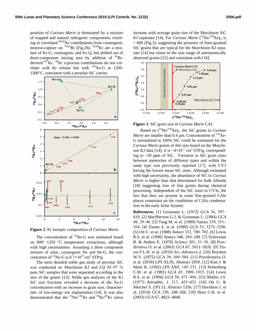
position of Curious Marie is dominated by a mixture

of trapped and natural radiogenic components, result-

ing in correlated 80,82Kr contributions from cosmogenic

neutron-capture on 79,81Br (Fig.2b). 83,84Kr are a mix-

ture of Kr-G, cosmogenic and Kr-Q, but shifted out of

three-component mixing area by addition of 81Br-

derived 82*Kr. 86Kr s-process contributions do not cor-

relate with Kr release but with 130Xe-G at 1200-

1300C, consistent with a presolar SiC carrier.

Figure 2. Kr isotopic composition of Curious Marie.

The concentration of 22Ne-G was estimated based

on 800‒1250 C temperature extractions, although

with high uncertainties. Assuming a three component

mixture of solar, cosmogenic Ne and Ne-G, the con-

centration of 22Ne-G is 0.7×10-8 cm3 STP/g.

The most detailed noble gas study of presolar SiC

was conducted on Murchison KJ and LQ 92‒97 %

pure SiC samples that were separated according to the

size of the grains [13]. Noble gas analyses of the KJ

SiC size fractions revealed a decrease of the Xe-G

concentration with an increase in grain size, character-

istic of low-energy ion implantation [14]. It was also

demonstrated that the 22Ne/130Xe and 86Kr/82Kr ratios

increase with average grain size of the Murchison SiC

KJ separates [14]. For Curious Marie (22Ne/130Xe)G is

~ 600 (Fig.3), suggesting the presence of finer-grained

SiC grains that are typical for the Murchison KJ sepa-

rate [14] but closer to the size range of astronomically

observed grains [15] and consistent with [16].

Figure 3. SiC grain size in Curious Marie CAI.

Based on (22Ne/130Xe)G, the SiC grains in Curious

Marie are smaller than 0.4 µm. Concentration of 132Xe-

G normalized to 100% SiC could be estimated for the

Curious Marie grains of this size based on the Murchi-

son KJ data [14]; it is ~4×10-7 cm3 STP/g, correspond-

ing to ~20 ppm of SiC. Variation in SiC grain sizes

between meteorites of different types and within the

same type was previously reported [17], with CV3

having the lowest mean SiC sizes. Although estimated

with high uncertainty, the abundance of SiC in Curious

Marie is higher than that determined for bulk Allende

[18] suggesting loss of fine grains during chemical

processing. Independent of the SiC sizes in CV3s, the

fact that they are present in some fine-grained CAIs

places constrains on the conditions of CAIs condensa-

tion in the early Solar System.

References: [1] Grossman L. (1972) GCA 36, 597‒

619. [2] MacPherson G.J. & Grossman L. (1984) GCA

48, 29‒46. [3] Tang M. et al. (1989) Nature 339, 351‒

354. [4] Zinner E. et al. (1989) GCA 53, 3273‒3290.

[5] Ott U. et al. (1988) Nature 332, 700‒702. [6] Lewis

R.S. et al. (1990) Nature 348, 293‒298. [7] Srinivasan

B. & Anders E. (1978) Science 201, 51‒56. [8] Prav-

divtseva O. et al. (2003) GCA 67, 5011‒5026. [9] Tis-

sot F.L.H. et al. (2016) Sci. Advances 2. [10] Boynton

W.V. (1975) GCA 39, 569‒584. [11] Pravdivtseva O.

et al. (2018) LPS XLIX, Abstract 2959. [12] Kim J. &

Marti K. (1992) LPS XXII, 145‒151. [13] Hohenberg

C.M. et al. (1981) GCA 45, 1909‒1915. [14] Lewis

R.S. et al. (1994) GCA 58, 471‒494. [15] Mathis J.S.

(1977) Astrophis. J. 217, 425‒433. [16] Ott U. &

Merchel S. LPS LI, Abstract 1356. [17] Davidson J. et

al. (2014) GCA 139, 248‒266. [18] Huss G.R. et al.

(2003) GCA 67, 4823‒4848.

80Kr/84Kr

0.29

0.3

0.31

0.32

0 3 6 9 12 15

86K

r/84

Kr

800

1400

1350

1300

10001100

11501200

1250

0

1

2

3

4

5

6

0 3 6 9 12 15

82K

r/84

Kr

1100

1150

1200

1250

1000

slope = 0.385 0.002

Kr-Q

-0.2

0.1

0.4

0.7

1.0

1.3

-0.5 0.5 1.5 2.5 3.5 4.584Kr/82Kr

83K

r/82

Kr

Kr-Q

Kr-cos

Kr-G1250

1000

1350

800

13001400

1150

1100

c

b

a

0.0

0.5

1.0

1.5

2.0

2.5

3.0

3.5

1.E+01 1.E+02 1.E+03 1.E+04 1.E+05 1.E+06

(22Ne/130Xe)G

(86K

r/8

2K

r)G

0.38 µm0.49 µm

0.67 µm

0.81 µm

1.14 µm

1.86 µm

3.02 µm

Murchison KJ [14]

astr

ono

mic

al o

bse

rvat

ion

s

Curious Marie CAI

& Murchison [16]


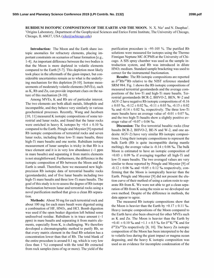
RUBIDIUM ISOTOPIC COMPOSITIONS OF THE EARTH AND THE MOON. N. X. Nie1 and N. Dauphas1. 1Origins Laboratory, Department of the Geophysical Sciences and Enrico Fermi Institute, The University of Chicago, Chicago, IL 60637, USA ([email protected])

Introduction: The Moon and the Earth share iso-

topic anomalies for refractory elements, placing im-portant constraints on scenarios of lunar formation [e.g., 1-4]. An important difference between the two bodies is that the Moon is more depleted in volatile elements compared to the Earth [5-7]. This depletion most likely took place in the aftermath of the giant-impact, but con-siderable uncertainties remain as to what is the underly-ing mechanism for this depletion [8-10]. Isotope meas-urements of moderately volatile elements (MVEs), such as K, Rb and Zn, can provide important clues on the na-ture of this mechanism [8-10].

Among MVEs, K and Rb are of particular interest. The two elements are both alkali metals, lithophile and incompatible, and they behave very similarly in various geochemical processes. Recently, Wang and Jacobsen [10, 11] measured K isotopic compositions of some ter-restrial and lunar rocks, and found that the lunar rocks were enriched in heavy K isotopes by +0.4 ± 0.10 ‰ compared to the Earth. Pringle and Moynier [9] reported Rb isotopic compositions of terrestrial rocks and seven lunar rocks, including three low-Ti mare basalts, three high-Ti mare basalts and one norite. Rubidium isotope measurement of lunar samples is tricky in that Rb is a trace element and it is in very low abundance (~1 ppm in mare basalts) and separating it from matrix elements is not straightforward. Furthermore, the difference in the isotopic composition of Rb between the Moon and the Earth is small. Therefore, here we measured new high-precision Rb isotopic data of terrestrial basaltic rocks (geostandards), and of five lunar basalts including two high-Ti mare basalts and three low-Ti mare basalts. The goal of this study is to re-assess the degree of Rb isotope fractionation between lunar and terrestrial rocks using a novel purification method that gives a clean Rb separa-tion.

Methods: About 50 mg for each terrestrial rock and about 100 mg for each mare basalt were digested using a combination of HF, HNO3, and HCl. Bomb digestion was used if the open beaker digestion left behind some undissolved residue. Rubidium is in trace amount (~1 ppm) in mare basalts and separating it from matrix ele-ments, especially from K, is challenging. We therefore developed a chromatographic method to purify Rb, so that every matrix element in the final Rb solution has a concentration lower than that of Rb. The total blank of the entire procedure is around 0.1 ng, which is very low (less than 1 %) compared with the total Rb extracted from rock samples (tens of ng or more). The yield of the

purification procedure is ~95-105 %. The purified Rb solutions were measured for isotopes using the Thermo Finnigan Neptune MC-ICPMS at the University of Chi-cago. A SIS spray chamber was used as the sample in-troduction system, and Rb was introduced in dilute HNO3 medium. Standard sample bracketing was used to correct for the instrumental fractionation.

Results: The Rb isotopic compositions are reported as d87Rb/85Rb relative to the NIST reference standard SRM 984. Fig. 1 shows the Rb isotopic compositions of measured terrestrial geostandards and the average com-positions of the low-Ti and high-Ti mare basalts. Ter-restrial geostandards BCR-2, BHVO-2, BEN, W-2 and AGV-2 have negative Rb isotopic compositions of -0.16 ± 0.03 ‰, -0.12 ± 0.02 ‰, -0.11 ± 0.03 ‰, -0.15 ± 0.02 ‰ and -0.14 ± 0.02 ‰, respectively. The three low-Ti mare basalts have an average value of -0.01 ± 0.07 ‰, and the two high-Ti basalts show a slightly positive av-erage value of +0.07 ± 0.06 ‰.

Discussion: The five terrestrial basaltic rocks (four basalts BCR-2, BHVO-2, BE-N and W-2, and one an-desite AGV-2) have very similar Rb isotopic composi-tions. Using their isotopic compositions to represent the bulk Earth (Rb is quite incompatible during mantle melting), the average value is -0.14 ± 0.06 ‰. The bulk Moon is estimated to have an isotopic composition of +0.03 ± 0.09 ‰ if averaging together all high-Ti and low-Ti mare basalts. The two averaged values are very similar to those reported by Pringle and Moynier [9] of -0.12 ± 0.06 ‰ and +0.05 ± 0.12 ‰ respectively, con-firming that the Moon is isotopically heavier than the Earth. Pringle and Moynier [9] did not present the elu-tion curve of their method of using a cation resin to sep-arate Rb from K. We were not able to get a clean sepa-ration of Rb from K using the resin so we developed our own method. Despite of the difference in methods, the data appear to agree.

The measured Rb isotopic compositions show that the Moon is heavier than the Earth by +0.17 ± 0.11 ‰. Heavy isotopic compositions of the Moon compared to the Earth have also been observed for other MVEs such as K and Zn. The Moon is heavier than the Earth by +0.41 ± 0.10 ‰ and +1.1 ± 0.5 ‰ for d41K/39K and for d66Zn/64Zn respectively [8, 10]. The heavy Zn isotopic composition of the Moon has been interpreted to be due to volatile loss during the giant impact or magma ocean degassing, and the heavy K isotopic composition was used as an evidence for incomplete condensation of the


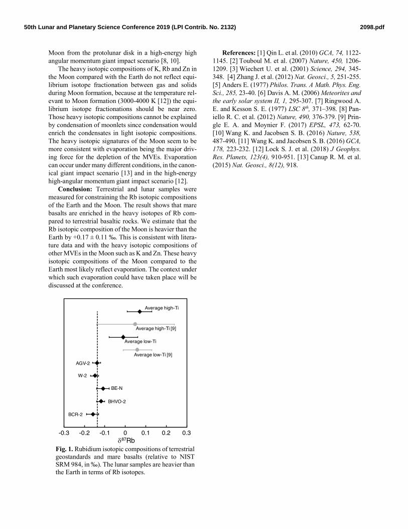
Moon from the protolunar disk in a high-energy high angular momentum giant impact scenario [8, 10].

The heavy isotopic compositions of K, Rb and Zn in the Moon compared with the Earth do not reflect equi-librium isotope fractionation between gas and solids during Moon formation, because at the temperature rel-evant to Moon formation (3000-4000 K [12]) the equi-librium isotope fractionations should be near zero. Those heavy isotopic compositions cannot be explained by condensation of moonlets since condensation would enrich the condensates in light isotopic compositions. The heavy isotopic signatures of the Moon seem to be more consistent with evaporation being the major driv-ing force for the depletion of the MVEs. Evaporation can occur under many different conditions, in the canon-ical giant impact scenario [13] and in the high-energy high-angular momentum giant impact scenario [12].

Conclusion: Terrestrial and lunar samples were measured for constraining the Rb isotopic compositions of the Earth and the Moon. The result shows that mare basalts are enriched in the heavy isotopes of Rb com-pared to terrestrial basaltic rocks. We estimate that the Rb isotopic composition of the Moon is heavier than the Earth by +0.17 ± 0.11 ‰. This is consistent with litera-ture data and with the heavy isotopic compositions of other MVEs in the Moon such as K and Zn. These heavy isotopic compositions of the Moon compared to the Earth most likely reflect evaporation. The context under which such evaporation could have taken place will be discussed at the conference.

References: [1] Qin L. et al. (2010) GCA, 74, 1122-1145. [2] Touboul M. et al. (2007) Nature, 450, 1206-1209. [3] Wiechert U. et al. (2001) Science, 294, 345-348. [4] Zhang J. et al. (2012) Nat. Geosci., 5, 251-255. [5] Anders E. (1977) Philos. Trans. A Math. Phys. Eng. Sci., 285, 23-40. [6] Davis A. M. (2006) Meteorites and the early solar system II, 1, 295-307. [7] Ringwood A. E. and Kesson S. E. (1977) LSC 8th, 371–398. [8] Pan-iello R. C. et al. (2012) Nature, 490, 376-379. [9] Prin-gle E. A. and Moynier F. (2017) EPSL, 473, 62-70. [10] Wang K. and Jacobsen S. B. (2016) Nature, 538, 487-490. [11] Wang K. and Jacobsen S. B. (2016) GCA, 178, 223-232. [12] Lock S. J. et al. (2018) J Geophys. Res. Planets, 123(4), 910-951. [13] Canup R. M. et al. (2015) Nat. Geosci., 8(12), 918.

Fig. 1. Rubidium isotopic compositions of terrestrial geostandards and mare basalts (relative to NIST SRM 984, in ‰). The lunar samples are heavier than the Earth in terms of Rb isotopes.

BCR-2

BHVO-2

BE-N

W-2

AGV-2

Average low-Ti

Average high-Ti

Average low-Ti [9]

Average high-Ti [9]

-0.3 -0.2 -0.1 0 0.1 0.2 0.3d87Rb


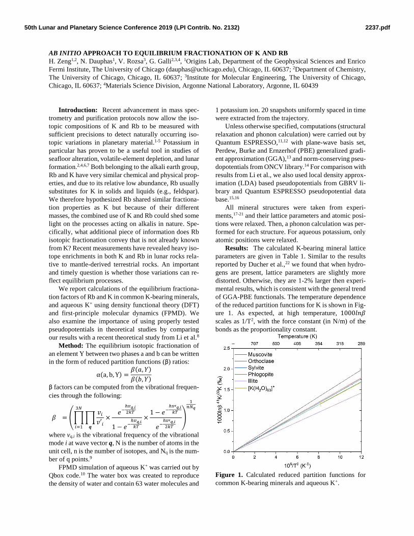
AB INITIO APPROACH TO EQUILIBRIUM FRACTIONATION OF K AND RB

H. Zeng1,2, N. Dauphas1, V. Rozsa3, G. Galli2,3,4, 1Origins Lab, Department of the Geophysical Sciences and Enrico

Fermi Institute, The University of Chicago ([email protected]), Chicago, IL 60637; 2Department of Chemistry,

The University of Chicago, Chicago, IL 60637; 3Institute for Molecular Engineering, The University of Chicago,

Chicago, IL 60637; 4Materials Science Division, Argonne National Laboratory, Argonne, IL 60439

Introduction: Recent advancement in mass spec-

trometry and purification protocols now allow the iso-

topic compositions of K and Rb to be measured with

sufficient precisions to detect naturally occurring iso-

topic variations in planetary material.1-5 Potassium in

particular has proven to be a useful tool in studies of

seafloor alteration, volatile-element depletion, and lunar

formation.2,4,6,7 Both belonging to the alkali earth group,

Rb and K have very similar chemical and physical prop-

erties, and due to its relative low abundance, Rb usually

substitutes for K in solids and liquids (e.g., feldspar).

We therefore hypothesized Rb shared similar fractiona-

tion properties as K but because of their different

masses, the combined use of K and Rb could shed some

light on the processes acting on alkalis in nature. Spe-

cifically, what additional piece of information does Rb

isotopic fractionation convey that is not already known

from K? Recent measurements have revealed heavy iso-

tope enrichments in both K and Rb in lunar rocks rela-

tive to mantle-derived terrestrial rocks. An important

and timely question is whether those variations can re-

flect equilibrium processes.

We report calculations of the equilibrium fractiona-

tion factors of Rb and K in common K-bearing minerals,

and aqueous K+ using density functional theory (DFT)

and first-principle molecular dynamics (FPMD). We

also examine the importance of using properly tested

pseudopotentials in theoretical studies by comparing

our results with a recent theoretical study from Li et al.8

Method: The equilibrium isotopic fractionation of

an element Y between two phases a and b can be written

in the form of reduced partition functions (β) ratios:

α(a, b, Y) =𝛽(𝑎, 𝑌)

𝛽(𝑏, 𝑌)

β factors can be computed from the vibrational frequen-

cies through the following:

𝛽 = (∏∏𝑣𝑖𝑣′𝑖

×𝑒−

ℎ𝑣𝑞,𝑖2𝑘𝑇

1 − 𝑒−ℎ𝑣𝑞,𝑖𝑘𝑇

×1 − 𝑒−

ℎ𝑣′𝑞,𝑖𝑘𝑇

𝑒−ℎ𝑣′𝑞,𝑖2𝑘𝑇𝒒

3𝑁

𝑖=1

)

1𝑛𝑁𝑞

where vq,i is the vibrational frequency of the vibrational

mode i at wave vector q, N is the number of atoms in the

unit cell, n is the number of isotopes, and Nq is the num-

ber of q points.9

FPMD simulation of aqueous K+ was carried out by

Qbox code.10 The water box was created to reproduce

the density of water and contain 63 water molecules and

1 potassium ion. 20 snapshots uniformly spaced in time

were extracted from the trajectory.

Unless otherwise specified, computations (structural

relaxation and phonon calculation) were carried out by

Quantum ESPRESSO,11,12 with plane-wave basis set,

Perdew, Burke and Ernzerhof (PBE) generalized gradi-

ent approximation (GGA),13 and norm-conserving pseu-

dopotentials from ONCV library.14 For comparison with

results from Li et al., we also used local density approx-

imation (LDA) based pseudopotentials from GBRV li-

brary and Quantum ESPRESSO pseudopotential data

base.15,16

All mineral structures were taken from experi-

ments,17-21 and their lattice parameters and atomic posi-

tions were relaxed. Then, a phonon calculation was per-

formed for each structure. For aqueous potassium, only

atomic positions were relaxed.

Results: The calculated K-bearing mineral lattice

parameters are given in Table 1. Similar to the results

reported by Ducher et al.,22 we found that when hydro-

gens are present, lattice parameters are slightly more

distorted. Otherwise, they are 1-2% larger then experi-

mental results, which is consistent with the general trend

of GGA-PBE functionals. The temperature dependence

of the reduced partition functions for K is shown in Fig-

ure 1. As expected, at high temperature, 1000𝑙𝑛𝛽

scales as 1/T2, with the force constant (in N/m) of the

bonds as the proportionality constant.

Figure 1. Calculated reduced partition functions for

common K-bearing minerals and aqueous K+.


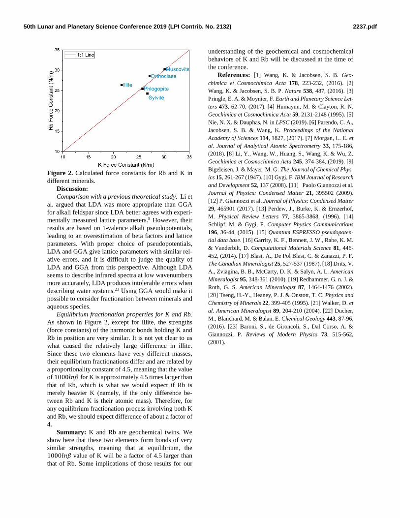
Figure 2. Calculated force constants for Rb and K in

different minerals.

Discussion:

Comparison with a previous theoretical study. Li et

al. argued that LDA was more appropriate than GGA

for alkali feldspar since LDA better agrees with experi-

mentally measured lattice parameters.8 However, their

results are based on 1-valence alkali pseudopotentials,

leading to an overestimation of beta factors and lattice

parameters. With proper choice of pseudopotentials,

LDA and GGA give lattice parameters with similar rel-

ative errors, and it is difficult to judge the quality of

LDA and GGA from this perspective. Although LDA

seems to describe infrared spectra at low wavenumbers

more accurately, LDA produces intolerable errors when

describing water systems.23 Using GGA would make it

possible to consider fractionation between minerals and

aqueous species.

Equilibrium fractionation properties for K and Rb.

As shown in Figure 2, except for illite, the strengths

(force constants) of the harmonic bonds holding K and

Rb in position are very similar. It is not yet clear to us

what caused the relatively large difference in illite.

Since these two elements have very different masses,

their equilibrium fractionations differ and are related by

a proportionality constant of 4.5, meaning that the value

of 1000𝑙𝑛𝛽 for K is approximately 4.5 times larger than

that of Rb, which is what we would expect if Rb is

merely heavier K (namely, if the only difference be-

tween Rb and K is their atomic mass). Therefore, for

any equilibrium fractionation process involving both K

and Rb, we should expect difference of about a factor of

4.

Summary: K and Rb are geochemical twins. We

show here that these two elements form bonds of very

similar strengths, meaning that at equilibrium, the

1000𝑙𝑛𝛽 value of K will be a factor of 4.5 larger than

that of Rb. Some implications of those results for our

understanding of the geochemical and cosmochemical

behaviors of K and Rb will be discussed at the time of

the conference.

References: [1] Wang, K. & Jacobsen, S. B. Geo-

chimica et Cosmochimica Acta 178, 223-232, (2016). [2]

Wang, K. & Jacobsen, S. B. P. Nature 538, 487, (2016). [3]

Pringle, E. A. & Moynier, F. Earth and Planetary Science Let-

ters 473, 62-70, (2017). [4] Humayun, M. & Clayton, R. N.

Geochimica et Cosmochimica Acta 59, 2131-2148 (1995). [5]

Nie, N. X. & Dauphas, N. in LPSC (2019). [6] Parendo, C. A.,

Jacobsen, S. B. & Wang, K. Proceedings of the National

Academy of Sciences 114, 1827, (2017). [7] Morgan, L. E. et

al. Journal of Analytical Atomic Spectrometry 33, 175-186,

(2018). [8] Li, Y., Wang, W., Huang, S., Wang, K. & Wu, Z.

Geochimica et Cosmochimica Acta 245, 374-384, (2019). [9]

Bigeleisen, J. & Mayer, M. G. The Journal of Chemical Phys-

ics 15, 261-267 (1947). [10] Gygi, F. IBM Journal of Research

and Development 52, 137 (2008). [11] Paolo Giannozzi et al.

Journal of Physics: Condensed Matter 21, 395502 (2009).

[12] P. Giannozzi et al. Journal of Physics: Condensed Matter

29, 465901 (2017). [13] Perdew, J., Burke, K. & Ernzerhof,

M. Physical Review Letters 77, 3865-3868, (1996). [14]

Schlipf, M. & Gygi, F. Computer Physics Communications

196, 36-44, (2015). [15] Quantum ESPRESSO pseudopoten-

tial data base. [16] Garrity, K. F., Bennett, J. W., Rabe, K. M.

& Vanderbilt, D. Computational Materials Science 81, 446-

452, (2014). [17] Blasi, A., De Pol Blasi, C. & Zanazzi, P. F.

The Canadian Mineralogist 25, 527-537 (1987). [18] Drits, V.

A., Zviagina, B. B., McCarty, D. K. & Salyn, A. L. American

Mineralogist 95, 348-361 (2010). [19] Redhammer, G. n. J. &

Roth, G. S. American Mineralogist 87, 1464-1476 (2002).

[20] Tseng, H.-Y., Heaney, P. J. & Onstott, T. C. Physics and

Chemistry of Minerals 22, 399-405 (1995). [21] Walker, D. et

al. American Mineralogist 89, 204-210 (2004). [22] Ducher,

M., Blanchard, M. & Balan, E. Chemical Geology 443, 87-96,

(2016). [23] Baroni, S., de Gironcoli, S., Dal Corso, A. &

Giannozzi, P. Reviews of Modern Physics 73, 515-562,

(2001).


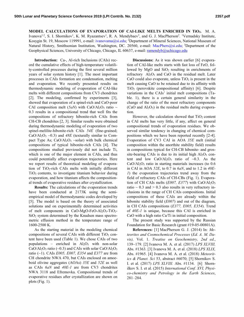
MODEL CALCULATIONS OF EVAPORATION OF CAI-LIKE MELTS ENRICHED IN TiO2. M. A. Ivanova1,2, S. I. Shornikov1, K. M. Ryazantsev1, R. A. Mendybaev3, and G. J. MacPherson2. 1Vernadsky Institute, Kosygin St. 19, Moscow 119991, e-mail: [email protected]; 2Department of Mineral Sciences, National Museum of Natural History, Smithsonian Institution, Washington, DC. 20560, e-mail: [email protected]; 3Department of the Geophysical Sciences, University of Chicago, Chicago, IL 60637, e-mail: [email protected]

Introduction: Ca-, Al-rich Inclusions (CAIs) rec-

ord the cumulative effects of high-temperature volatili-ty-controlled processes during the first several million years of solar system history [1]. The most important processes in CAIs formation are condensation, melting and evaporation. We recently presented results on thermodynamic modeling of evaporation of CAI-like melts with different compositions from CV3 chondrites [2]. The modeling, confirmed by experiments [3], showed that evaporation of a spinel-rich and CaO-poor CAI composition melt (5aN) with CaO/Al2O3 ratio ~ 0.3 results in a compositional trend that well fits the compositions of refractory hibonite-rich CAIs from CH-CB chondrites [2, 3]. Similar results were obtained during thermodynamic modeling of evaporation of two spinel-melilite-hibonite-rich CAIs 54E (fine-grained; CaO/Al2O3 ~0.3) and 48E (texturally similar to Com-pact Type As; CaO/Al2O3 ~solar) with bulk chemical compositions of typical hibonite-rich CAIs [4]. The compositions studied previously did not include Ti, which is one of the major element in CAIs, and thus could potentially affect evaporation trajectories. Here we report results of theoretical modeling of evapora-tion of TiO2-rich CAIs melts with initially different TiO2 contents, to investigate titanium behavior during evaporation, and how titanium affects the composition-al trends of evaporative residues after crystallization.

Results: The calculations of the evaporation trends have been conducted at 2173K using the semi-empirical model of thermodynamic codes developed by [5]. The model is based on the theory of associated solutions and on experimentally determined activities of melt components in CaO-MgO-FeO-Al2O3-TiO2-SiO2 system determined by the Knudsen mass spectro-metric effusion method in the temperature range of 1600-2500 K.

As the starting material in the modeling chemical compositions of several CAIs with different TiO2 con-tent have been used (Table 1). We chose CAIs of two populations – enriched in Al2O3 with non-solar CaO/Al2O3 ratio (~0.3) and CAIs with solar CaO/Al2O3 ratio (~1). CAIs E005, E007, E354 and E377 are from CH chondrite NWA 470, but CAIs enclosed on amoe-boid olivine aggregates (AOAs) 35E and 52E as well as CAIs 6aN and 40E-1 are from CV3 chondrites NWA 3118 and Efremovka. Compositional trends of evaporative residues after crystallization are shown on plots (Fig. 1).

Discussions: As it was shown earlier [6] evapora-tion of CAI-like melts starts with fast loss of FeO, fol-lowed by MgO and SiO2 resulting in enrichments of refractory Al2O3 and CaO in the residual melt. Later CaO could also evaporate, unless TiO2 is present in the melt causing CaO to be retained due to its affinity with TiO2 (perovskite compositional affinity) [6]. Despite variations in the CAIs’ initial melt compositions (Ta-ble. 1), there is a certain general similarity in the change of the ratio of the most refractory components (CaO and Al2O3) in the residual melts during evapora-tion.

However, the calculation showed that TiO2 content in CAI melts has very little, if any, affect on general compositional trends of evaporation residues. We ob-served similar tendency in changing of chemical com-positions which we have been reported recently [2-4]. Evaporation of CV3 CAI in AOA 35E melt (initial composition within the anorthite stability field) results in compositions typical for CH-CB hibonite- and gros-site-bearing CAIs is due to its initial high Al2O3 con-tent and low CaO/Al2O3 ratio of ~0.3. As the CaO/Al2O3 ratio in starting materials increases (to 0.6 in CAI in AOA 52E, to 0.7 in 6aN, and to 1.2 in 40E-1) the evaporation trajectories trend away from the field of refractory CAIs of CH-CBs (Fig. 1). Evapora-tion of CH CAIs melts (E007, E377) with CaO/Al2O3 ratio ~ 0.3 and > 0.3 also results in very refractory in-clusions in the range of CH CAIs compositions. Initial compositions of these CAIs are already within the hibonite stability field (E007) and out of the diagram, in CH CAIs compositions (E377, E005, E354). Trend of 40E-1 is unique, because this CAI is enriched in CaO with a high ratio Ca/Ti in initial composition.

The present study was supported by the Russian Foundation for Basic Research (grant #19-05-00801A).

References: [1] MacPherson G. J. (2014) In: Me-teorites and Cosmochemical Processes (Ed. A. M. Da-vis), Vol. 1. Treatise on Geochemistry, 2nd ed., 139−179. [2] Ivanova M. A. et al. (2017) LPS XLVIII, Abs. #1363. [3] Ivanova M. A. et al. (2018) LPS XLIX, Abs. #1965. [4] Ivanova M. A. et al. (2018) Meteorit-ics & Planet. Sci 53, abstract #6070; [5] Shornikov S. I. et al. (2017) LPS XLVIII. Abs. #1134. [6] Shorn-ilkov S. I. et al. (2015) International Conf. XVI, Physi-co-chemistry and Petrology in the Earth Sciences, 281–284.





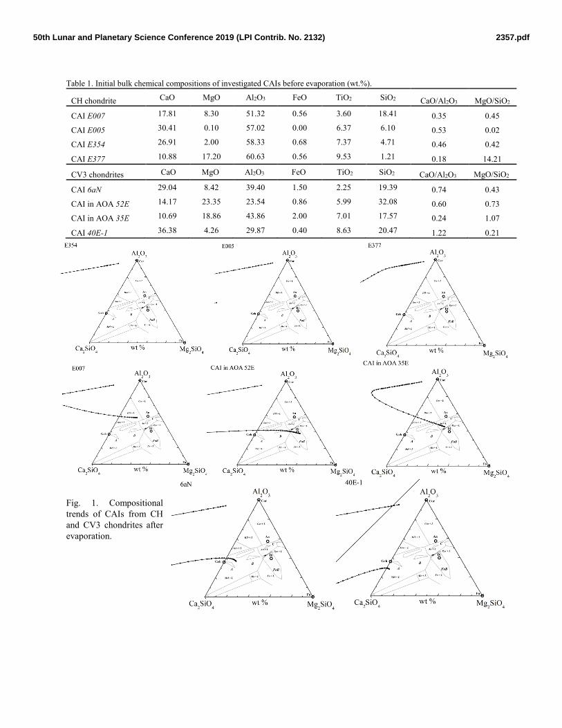
Table 1. Initial bulk chemical compositions of investigated CAIs before evaporation (wt.%).

CH chondrite CaO MgO Al2O3 FeO TiO2 SiO2 CaO/Al2O3 MgO/SiO2

CAI E007 17.81 8.30 51.32 0.56 3.60 18.41 0.35 0.45

CAI E005 30.41 0.10 57.02 0.00 6.37 6.10 0.53 0.02

CAI E354 26.91 2.00 58.33 0.68 7.37 4.71 0.46 0.42

CAI E377 10.88 17.20 60.63 0.56 9.53 1.21 0.18 14.21

CV3 chondrites CaO MgO Al2O3 FeO TiO2 SiO2 CaO/Al2O3 MgO/SiO2

CAI 6aN 29.04 8.42 39.40 1.50 2.25 19.39 0.74 0.43

CAI in AOA 52E 14.17 23.35 23.54 0.86 5.99 32.08 0.60 0.73

CAI in AOA 35E 10.69 18.86 43.86 2.00 7.01 17.57 0.24 1.07

CAI 40E-1 36.38 4.26 29.87 0.40 8.63 20.47 1.22 0.21

Fig. 1. Compositional trends of CAIs from CH and CV3 chondrites after evaporation.


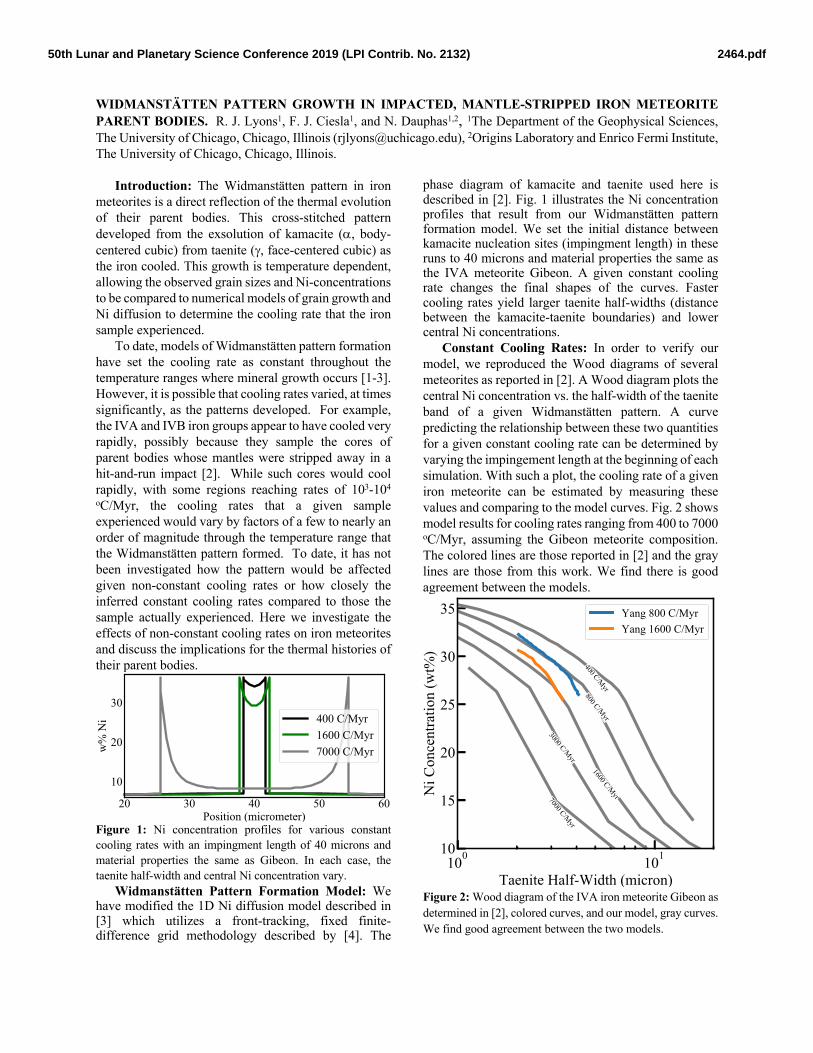
WIDMANSTÄTTEN PATTERN GROWTH IN IMPACTED, MANTLE-STRIPPED IRON METEORITE PARENT BODIES. R. J. Lyons1, F. J. Ciesla1, and N. Dauphas1,2, 1The Department of the Geophysical Sciences, The University of Chicago, Chicago, Illinois ([email protected]), 2Origins Laboratory and Enrico Fermi Institute, The University of Chicago, Chicago, Illinois.

Introduction: The Widmanstätten pattern in iron meteorites is a direct reflection of the thermal evolution of their parent bodies. This cross-stitched pattern developed from the exsolution of kamacite (a, body-centered cubic) from taenite (g, face-centered cubic) as the iron cooled. This growth is temperature dependent, allowing the observed grain sizes and Ni-concentrations to be compared to numerical models of grain growth and Ni diffusion to determine the cooling rate that the iron sample experienced.

To date, models of Widmanstätten pattern formation have set the cooling rate as constant throughout the temperature ranges where mineral growth occurs [1-3]. However, it is possible that cooling rates varied, at times significantly, as the patterns developed. For example, the IVA and IVB iron groups appear to have cooled very rapidly, possibly because they sample the cores of parent bodies whose mantles were stripped away in a hit-and-run impact [2]. While such cores would cool rapidly, with some regions reaching rates of 103-104 oC/Myr, the cooling rates that a given sample experienced would vary by factors of a few to nearly an order of magnitude through the temperature range that the Widmanstätten pattern formed. To date, it has not been investigated how the pattern would be affected given non-constant cooling rates or how closely the inferred constant cooling rates compared to those the sample actually experienced. Here we investigate the effects of non-constant cooling rates on iron meteorites and discuss the implications for the thermal histories of their parent bodies.

Figure 1: Ni concentration profiles for various constant cooling rates with an impingment length of 40 microns and material properties the same as Gibeon. In each case, the taenite half-width and central Ni concentration vary.

Widmanstätten Pattern Formation Model: We have modified the 1D Ni diffusion model described in [3] which utilizes a front-tracking, fixed finite-difference grid methodology described by [4]. The

phase diagram of kamacite and taenite used here is described in [2]. Fig. 1 illustrates the Ni concentration profiles that result from our Widmanstätten pattern formation model. We set the initial distance between kamacite nucleation sites (impingment length) in these runs to 40 microns and material properties the same as the IVA meteorite Gibeon. A given constant cooling rate changes the final shapes of the curves. Faster cooling rates yield larger taenite half-widths (distance between the kamacite-taenite boundaries) and lower central Ni concentrations.

Constant Cooling Rates: In order to verify our model, we reproduced the Wood diagrams of several meteorites as reported in [2]. A Wood diagram plots the central Ni concentration vs. the half-width of the taenite band of a given Widmanstätten pattern. A curve predicting the relationship between these two quantities for a given constant cooling rate can be determined by varying the impingement length at the beginning of each simulation. With such a plot, the cooling rate of a given iron meteorite can be estimated by measuring these values and comparing to the model curves. Fig. 2 shows model results for cooling rates ranging from 400 to 7000 oC/Myr, assuming the Gibeon meteorite composition. The colored lines are those reported in [2] and the gray lines are those from this work. We find there is good agreement between the models.

Figure 2: Wood diagram of the IVA iron meteorite Gibeon as determined in [2], colored curves, and our model, gray curves. We find good agreement between the two models.


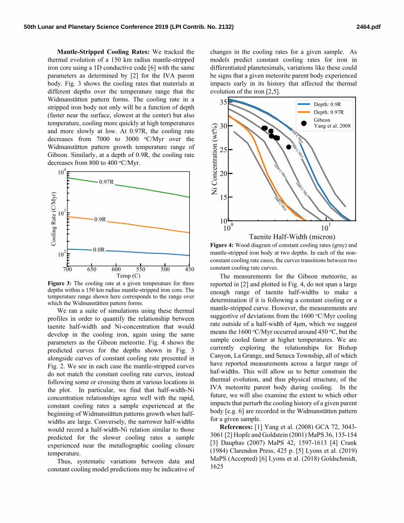
Mantle-Stripped Cooling Rates: We tracked the thermal evolution of a 150 km radius mantle-stripped iron core using a 1D conductive code [6] with the same parameters as determined by [2] for the IVA parent body. Fig. 3 shows the cooling rates that materials at different depths over the temperature range that the Widmanstätten pattern forms. The cooling rate in a stripped iron body not only will be a function of depth (faster near the surface, slowest at the center) but also temperature, cooling more quickly at high temperatures and more slowly at low. At 0.97R, the cooling rate decreases from 7000 to 3000 oC/Myr over the Widmanstätten pattern growth temperature range of Gibeon. Similarly, at a depth of 0.9R, the cooling rate decreases from 800 to 400 oC/Myr.

Figure 3: The cooling rate at a given temperature for three depths within a 150 km radius mantle-stripped iron core. The temperature range shown here corresponds to the range over which the Widmanstätten pattern forms.

We ran a suite of simulations using these thermal profiles in order to quantify the relationship between taenite half-width and Ni-concentration that would develop in the cooling iron, again using the same parameters as the Gibeon meteorite. Fig. 4 shows the predicted curves for the depths shown in Fig. 3 alongside curves of constant cooling rate presented in Fig. 2. We see in each case the mantle-stripped curves do not match the constant cooling rate curves, instead following some or crossing them at various locations in the plot. In particular, we find that half-width-Ni concentration relationships agree well with the rapid, constant cooling rates a sample experienced at the beginning of Widmanstätten patterns growth when half-widths are large. Conversely, the narrower half-widths would record a half-width-Ni relation similar to those predicted for the slower cooling rates a sample experienced near the metallographic cooling closure temperature.

Thus, systematic variations between data and constant cooling model predictions may be indicative of

changes in the cooling rates for a given sample. As models predict constant cooling rates for iron in differentiated planetesimals, variations like these could be signs that a given meteorite parent body experienced impacts early in its history that affected the thermal evolution of the iron [2,5].

Figure 4: Wood diagram of constant cooling rates (gray) and mantle-stripped iron body at two depths. In each of the non-constant cooling rate cases, the curves transitions between two constant cooling rate curves.

The measurements for the Gibeon meteorite, as reported in [2] and plotted in Fig. 4, do not span a large enough range of taenite half-widths to make a determination if it is following a constant cooling or a mantle-stripped curve. However, the measurements are suggestive of deviations from the 1600 oC/Myr cooling rate outside of a half-width of 4μm, which we suggest means the 1600 oC/Myr occurred around 450 oC, but the sample cooled faster at higher temperatures. We are currently exploring the relationships for Bishop Canyon, La Grange, and Seneca Township, all of which have reported measurements across a larger range of haf-widths. This will allow us to better constrain the thermal evolution, and thus physical structure, of the IVA meteorite parent body during cooling. In the future, we will also examine the extent to which other impacts that perturb the cooling history of a given parent body [e.g. 6] are recorded in the Widmanstätten pattern for a given sample.

References: [1] Yang et al. (2008) GCA 72, 3043-3061 [2] Hopfe and Goldstein (2001) MaPS 36, 135-154 [3] Dauphas (2007) MaPS 42, 1597-1613 [4] Crank (1984) Clarendon Press, 425 p. [5] Lyons et al. (2019) MaPS (Accepted) [6] Lyons et al. (2018) Goldschmidt, 1625


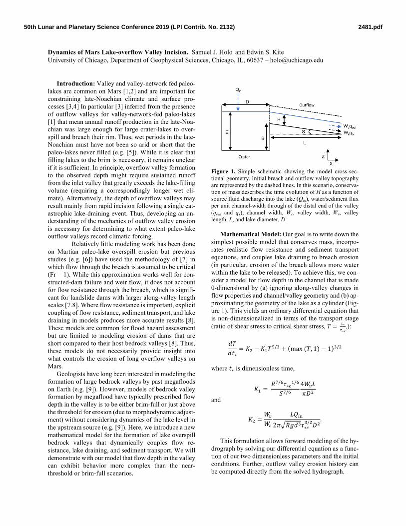
Dynamics of Mars Lake-overflow Valley Incision. Samuel J. Holo and Edwin S. Kite University of Chicago, Department of Geophysical Sciences, Chicago, IL, 60637 – [email protected]

Introduction: Valley and valley-network fed paleo-

lakes are common on Mars [1,2] and are important for constraining late-Noachian climate and surface pro-cesses [3,4] In particular [3] inferred from the presence of outflow valleys for valley-network-fed paleo-lakes [1] that mean annual runoff production in the late-Noa-chian was large enough for large crater-lakes to over-spill and breach their rim. Thus, wet periods in the late-Noachian must have not been so arid or short that the paleo-lakes never filled (e.g. [5]). While it is clear that filling lakes to the brim is necessary, it remains unclear if it is sufficient. In principle, overflow valley formation to the observed depth might require sustained runoff from the inlet valley that greatly exceeds the lake-filling volume (requiring a correspondingly longer wet cli-mate). Alternatively, the depth of overflow valleys may result mainly from rapid incision following a single cat-astrophic lake-draining event. Thus, developing an un-derstanding of the mechanics of outflow valley erosion is necessary for determining to what extent paleo-lake outflow valleys record climatic forcing.

Relatively little modeling work has been done on Martian paleo-lake overspill erosion but previous studies (e.g. [6]) have used the methodology of [7] in which flow through the breach is assumed to be critical (Fr = 1). While this approximation works well for con-structed-dam failure and weir flow, it does not account for flow resistance through the breach, which is signifi-cant for landslide dams with larger along-valley length scales [7.8]. Where flow resistance is important, explicit coupling of flow resistance, sediment transport, and lake draining in models produces more accurate results [8]. These models are common for flood hazard assessment but are limited to modeling erosion of dams that are short compared to their host bedrock valleys [8]. Thus, these models do not necessarily provide insight into what controls the erosion of long overflow valleys on Mars.

Geologists have long been interested in modeling the formation of large bedrock valleys by past megafloods on Earth (e.g. [9]). However, models of bedrock valley formation by megaflood have typically prescribed flow depth in the valley is to be either brim-full or just above the threshold for erosion (due to morphodynamic adjust-ment) without considering dynamics of the lake level in the upstream source (e.g. [9]). Here, we introduce a new mathematical model for the formation of lake overspill bedrock valleys that dynamically couples flow re-sistance, lake draining, and sediment transport. We will demonstrate with our model that flow depth in the valley can exhibit behavior more complex than the near-threshold or brim-full scenarios.

Figure 1. Simple schematic showing the model cross-sec-tional geometry. Initial breach and outflow valley topography are represented by the dashed lines. In this scenario, conserva-tion of mass describes the time evolution of H as a function of source fluid discharge into the lake (Qin), water/sediment flux per unit channel-width through of the distal end of the valley (qout and qs), channel width, Wc, valley width, Wv, valley length, L, and lake diameter, D

Mathematical Model: Our goal is to write down the

simplest possible model that conserves mass, incorpo-rates realistic flow resistance and sediment transport equations, and couples lake draining to breach erosion (in particular, erosion of the breach allows more water within the lake to be released). To achieve this, we con-sider a model for flow depth in the channel that is made 0-dimensional by (a) ignoring along-valley changes in flow properties and channel/valley geometry and (b) ap-proximating the geometry of the lake as a cylinder (Fig-ure 1). This yields an ordinary differential equation that is non-dimensionalized in terms of the transport stage (ratio of shear stress to critical shear stress, 𝑇 = $∗

$∗&,):

𝑑𝑇𝑑𝑡∗

= 𝐾* − 𝐾,𝑇-// + max(𝑇, 1) − 1 //*

where 𝑡∗ is dimensionless time,

𝐾, = 𝑅9/:𝜏∗<,/:

𝑆9/:4𝑊@𝐿𝜋𝐷*

and

𝐾* =𝑊@

𝑊<

𝐿𝑄EF2𝜋 𝑅𝑔𝑑/𝜏∗<

//*𝐷*.

This formulation allows forward modeling of the hy-

drograph by solving our differential equation as a func-tion of our two dimensionless parameters and the initial conditions. Further, outflow valley erosion history can be computed directly from the solved hydrograph.


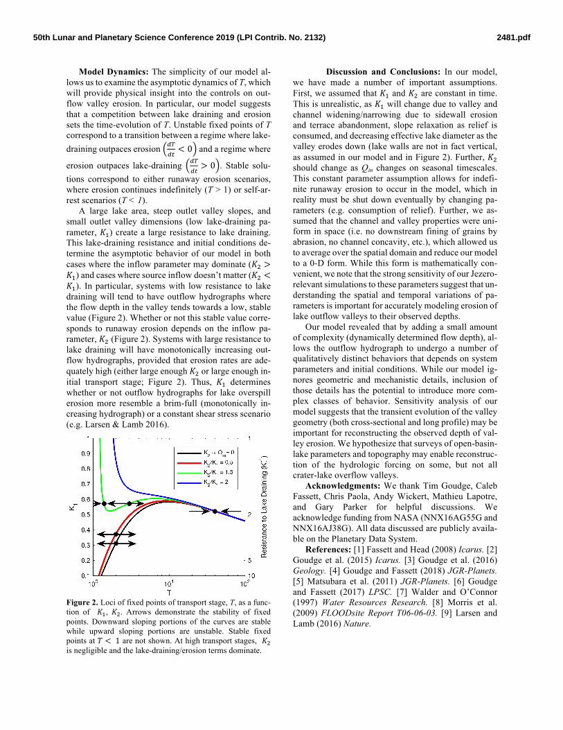
Model Dynamics: The simplicity of our model al-lows us to examine the asymptotic dynamics of T, which will provide physical insight into the controls on out-flow valley erosion. In particular, our model suggests that a competition between lake draining and erosion sets the time-evolution of T. Unstable fixed points of T correspond to a transition between a regime where lake-draining outpaces erosion JK

JL< 0 and a regime where

erosion outpaces lake-draining JKJL> 0 . Stable solu-

tions correspond to either runaway erosion scenarios, where erosion continues indefinitely (T > 1) or self-ar-rest scenarios (T < 1).

A large lake area, steep outlet valley slopes, and small outlet valley dimensions (low lake-draining pa-rameter, 𝐾,) create a large resistance to lake draining. This lake-draining resistance and initial conditions de-termine the asymptotic behavior of our model in both cases where the inflow parameter may dominate (𝐾* >𝐾,) and cases where source inflow doesn’t matter (𝐾* <𝐾,). In particular, systems with low resistance to lake draining will tend to have outflow hydrographs where the flow depth in the valley tends towards a low, stable value (Figure 2). Whether or not this stable value corre-sponds to runaway erosion depends on the inflow pa-rameter, 𝐾* (Figure 2). Systems with large resistance to lake draining will have monotonically increasing out-flow hydrographs, provided that erosion rates are ade-quately high (either large enough 𝐾* or large enough in-itial transport stage; Figure 2). Thus, 𝐾, determines whether or not outflow hydrographs for lake overspill erosion more resemble a brim-full (monotonically in-creasing hydrograph) or a constant shear stress scenario (e.g. Larsen & Lamb 2016).

Figure 2. Loci of fixed points of transport stage, T, as a func-tion of 𝐾,, 𝐾*. Arrows demonstrate the stability of fixed points. Downward sloping portions of the curves are stable while upward sloping portions are unstable. Stable fixed points at 𝑇 < 1 are not shown. At high transport stages, 𝐾* is negligible and the lake-draining/erosion terms dominate.

Discussion and Conclusions: In our model, we have made a number of important assumptions. First, we assumed that 𝐾, and 𝐾* are constant in time. This is unrealistic, as 𝐾, will change due to valley and channel widening/narrowing due to sidewall erosion and terrace abandonment, slope relaxation as relief is consumed, and decreasing effective lake diameter as the valley erodes down (lake walls are not in fact vertical, as assumed in our model and in Figure 2). Further, 𝐾* should change as Qin changes on seasonal timescales. This constant parameter assumption allows for indefi-nite runaway erosion to occur in the model, which in reality must be shut down eventually by changing pa-rameters (e.g. consumption of relief). Further, we as-sumed that the channel and valley properties were uni-form in space (i.e. no downstream fining of grains by abrasion, no channel concavity, etc.), which allowed us to average over the spatial domain and reduce our model to a 0-D form. While this form is mathematically con-venient, we note that the strong sensitivity of our Jezero-relevant simulations to these parameters suggest that un-derstanding the spatial and temporal variations of pa-rameters is important for accurately modeling erosion of lake outflow valleys to their observed depths.

Our model revealed that by adding a small amount of complexity (dynamically determined flow depth), al-lows the outflow hydrograph to undergo a number of qualitatively distinct behaviors that depends on system parameters and initial conditions. While our model ig-nores geometric and mechanistic details, inclusion of those details has the potential to introduce more com-plex classes of behavior. Sensitivity analysis of our model suggests that the transient evolution of the valley geometry (both cross-sectional and long profile) may be important for reconstructing the observed depth of val-ley erosion. We hypothesize that surveys of open-basin-lake parameters and topography may enable reconstruc-tion of the hydrologic forcing on some, but not all crater-lake overflow valleys.

Acknowledgments: We thank Tim Goudge, Caleb Fassett, Chris Paola, Andy Wickert, Mathieu Lapotre, and Gary Parker for helpful discussions. We acknowledge funding from NASA (NNX16AG55G and NNX16AJ38G). All data discussed are publicly availa-ble on the Planetary Data System.

References: [1] Fassett and Head (2008) Icarus. [2] Goudge et al. (2015) Icarus. [3] Goudge et al. (2016) Geology. [4] Goudge and Fassett (2018) JGR-Planets. [5] Matsubara et al. (2011) JGR-Planets. [6] Goudge and Fassett (2017) LPSC. [7] Walder and O’Connor (1997) Water Resources Research. [8] Morris et al. (2009) FLOODsite Report T06-06-03. [9] Larsen and Lamb (2016) Nature.


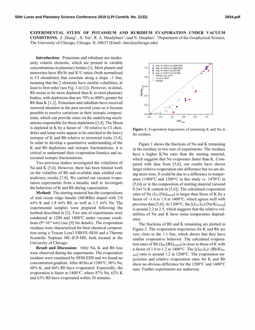
EXPERIMENTAL STUDY OF POTASSIUM AND RUBIDIUM EVAPORATION UNDER VACUUM

CONDITIONS. Z. Zhang1 , X. Nie1, R. A. Mendybaev1, and N. Dauphas1. 1Department of the Geophysical Science,

The University of Chicago, Chicago, IL 60637 (Email: [email protected])

Introduction: Potassium and rubidium are moder-

ately volatile elements, which are present in variable

concentrations in planetary bodies [1]. Most planets and

meteorites have Rb/Sr and K/U ratios (both normalized

to CI chondrites) that correlate along a slope ~1 line,

meaning that the 2 elements have similar volatilities, at

least to first order (see Fig. 3 in [1]). However, in detail,

Rb seems to be more depleted than K in most planetary

bodies, with depletions that are 70% to 400% greater for

Rb than K [1,2]. Potassium and rubidium have received

renewed attention in the past several years as it became

possible to resolve variations in their isotopic composi-

tions, which can provide clues on the underlying mech-

anisms responsible for those depletions [3,4]. The Moon

is depleted in K by a factor of ~30 relative to CI chon-

drites and lunar rocks appear to be enriched in the heavy

isotopes of K and Rb relative to terrestrial rocks [3,4].

In order to develop a quantitative understanding of the

K and Rb depletions and isotopic fractionations, it is

critical to understand their evaporation kinetics and as-

sociated isotopic fractionations.

Two previous studies investigated the volatilities of

Na and K [5,6]. However, there has been limited work

on the volatility of Rb and available data yielded con-

tradictory results [7,8]. We carried out vacuum evapo-

ration experiments from a basaltic melt to investigate

the behaviors of K and Rb during vaporization.

Method: The starting material has the compositions

of mid ocean ridge basalts (MORBs) doped with 2.0

wt% K and 1.8 wt% Rb, as well as 1.3 wt% Na. The

experimental samples were prepared following the

method described in [3]. Two sets of experiments were

conducted at 1200 and 1400°C under vacuum condi-

tions (P=10-6 torr) (see [9] for details). The evaporation

residues were characterized for their chemical composi-

tion using a Tescan Lyra3 FIB/FE-SEM and a Thermo

Scientific Neptune MC-ICP-MS, both located at the

University of Chicago.

Result and Discussion: Only Na, K and Rb loss

were observed during the experiments. The evaporation

residues were examined by SEM-EDS and we found no

concentration gradient. After 40 hrs at 1200°C, 96% Na,

60% K, and 66% Rb have evaporated. Expectedly, the

evaporation is faster at 1400°C, where 87% Na, 62% K

and 63% Rb have evaporated within 30 minutes.

Figure 1. Evaporation trajectories of remaining K and Na in

the residues.

Figure 1 shows the fractions of Na and K remaining

in the residues in two sets of experiments. The residues

have a higher K/Na ratio than the starting material,

which suggests that Na evaporates faster than K. Com-

pared with data from [5,6], our results have shown

larger relative evaporation rate difference but we are do-

ing more tests. It could be due to a difference in temper-

ature (1400°C and 1200°C in this study vs. 1470°C in

[5,6]) or in the composition of starting material (around

0.3wt % K content in [5,6]). The calculated evaporation

rates of Na (JNa/[Na]initial) is larger than those of K by a

factor of ~1.6 to 1.8 at 1400°C, which agrees well with

previous data [5,6]. At 1200°C, the [(JNa/JK)/(Na/K)initial]

is around 2.2 to 2.5, which suggests that the relative vol-

atilities of Na and K have some temperature depend-

ence.

The fractions of Rb and K remaining are plotted in

Figure 2. The evaporation trajectories for K and Rb are

very close to the 1:1 line, which shows that they have

similar evaporative behavior. The calculated evapora-

tion rates of Rb (JRb/[Rb]initial) is close to those of K with

a factor of 1.0 to 1.2 at 1400°C. The [(JRb/JK)/ (Rb/K)in-

itial] ratio is around 1.2 at 1200°C. The evaporation tra-

jectories and relative evaporation rates for K and Rb

show no obvious difference for the 1200°C and 1400°C

runs. Further experiments are underway.

0.0 0.2 0.4 0.6 0.8 1.0

0.0

0.2

0.4

0.6

0.8

1.0

Exp. at 1400°C by ICP-MS

Exp. at 1200°C by ICP-MS

Richter et al. 2011

Yu et al. 2003

Na/Na0

Na

/Na

initia

l

K/Kinitial

Exp. at 1200°C by SEM-EDS

Exp. at 1400°C by SEM-EDS


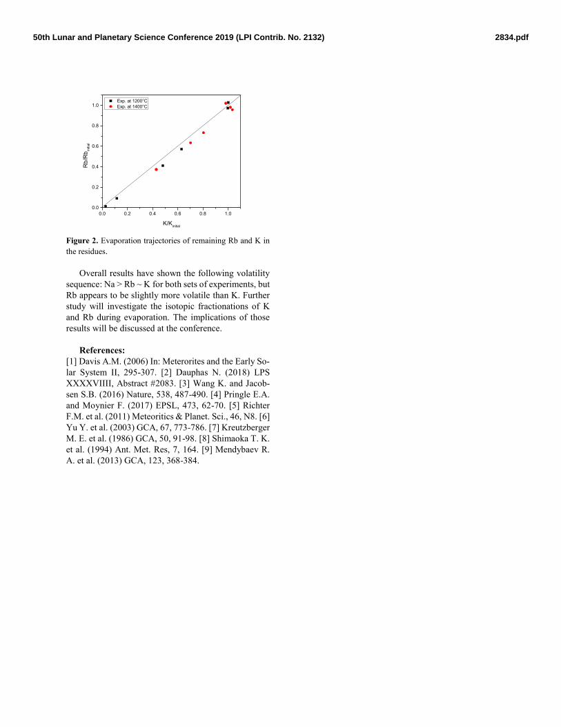
Figure 2. Evaporation trajectories of remaining Rb and K in

the residues.

Overall results have shown the following volatility

sequence: Na > Rb ~ K for both sets of experiments, but

Rb appears to be slightly more volatile than K. Further

study will investigate the isotopic fractionations of K

and Rb during evaporation. The implications of those

results will be discussed at the conference.

References:

[1] Davis A.M. (2006) In: Meterorites and the Early So-

lar System II, 295-307. [2] Dauphas N. (2018) LPS

XXXXVIIII, Abstract #2083. [3] Wang K. and Jacob-

sen S.B. (2016) Nature, 538, 487-490. [4] Pringle E.A.

and Moynier F. (2017) EPSL, 473, 62-70. [5] Richter

F.M. et al. (2011) Meteoritics & Planet. Sci., 46, N8. [6]

Yu Y. et al. (2003) GCA, 67, 773-786. [7] Kreutzberger

M. E. et al. (1986) GCA, 50, 91-98. [8] Shimaoka T. K.

et al. (1994) Ant. Met. Res, 7, 164. [9] Mendybaev R.

A. et al. (2013) GCA, 123, 368-384.

0.0 0.2 0.4 0.6 0.8 1.0

0.0

0.2

0.4

0.6

0.8

1.0

Exp. at 1200°C

Exp. at 1400°C

Rb

/Rb

initia

l

K/Kinitial


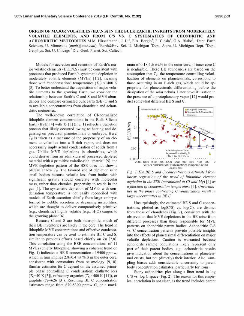
ORIGIN OF MAJOR VOLATILES (H,C,N,S) IN THE BULK EARTH: INSIGHTS FROM MODERATELY VOLATILE ELEMENTS, AND FROM C/S VS. C SYSTEMATICS OF CHONDRITIC AND ACHONDRITIC METEORITES M.M. Hirschmann1, J. Li2, E.A. Bergin3, F. Ciesla4, G.A. Blake5, 1Dept. Earth Sciences, U. Minnesota ([email protected]), 2Earth&Env. Sci. U. Michigan 3Dept. Astro. U. Michigan Dept. 4Dept. Geophys. Sci. U. Chicago 5Div. Geol. Planet. Sci. Caltech.

Models for accretion and retention of Earth’s ma-

jor volatile elements (H,C,N,S) must be consistent with processes that produced Earth’s systematic depletion in moderately volatile elements (MVEs) [1,2], meaning those with “condensation” temperatures (TC) <1400 K [3]. To better understand the acquisition of major vola-tile elements to the growing Earth, we consider the relationship between Earth’s C and S and MVE abun-dances and compare estimated bulk earth (BE) C and S to available concentrations from chondritic and achon-dritic meteorites.

The well-known correlation of CI-normalized lithophile element concentrations in the Bulk Silicate Earth (BSE) [4] with TC [3] (Fig. 1) reflects a depletion process that likely occurred owing to heating and de-gassing on precursor planetesimals or embryos. Here, TC is taken as a measure of the propensity of an ele-ment to volatilize into a H-rich vapor, and does not necessarily imply actual condensation of solids from a gas. Unlike MVE depletions in chondrites, which could derive from an admixture of processed depleted material with a primitive volatile-rich “matrix” [5], the MVE depletion pattern of the BSE does not show a plateau at low TC. The favored site of depletion is in small bodies because volatile loss from bodies with significant gravity should correlate with molecular mass, rather than chemical propensity to reside in the gas [1]. The systematic depletion of MVEs with con-densation temperature is not easily reconciled with models of Earth accretion chiefly from large embryos formed by pebble accretion or streaming instabilities, which are thought to deliver comparatively primitive (e.g., chondritic) highly volatile (e.g,. H2O) cargos to the growing planet [6].

Because C and S are both siderophile, much of their BE inventories are likely in the core. The trend in lithophile MVE concentrations and effective condensa-tion temperature can be used to estimate BE C and S, similar to previous efforts based chiefly on Zn [7,8]. This correlation using the BSE concentrations of 11 MVEs (chiefly lithophile, showing a coherent trend on Fig. 1) indicates a BE S concentration of 9400 ppmw, which in turn implies 2.8±0.4 wt.% S in the outer core, consistent with constraints from seismology [9,10]. Similar estimates for C depend on the assumed princi-ple phase controlling C condensation: clathrate ices (TC=40 K [3]), refractory organics (TC ~400 K [11]), or graphite (TC=626 [3]). Resulting BE C concentration estimates range from 670-5300 ppmw C, or a maxi-

mum of 0.18-1.6 wt.% in the outer core, if inner core C is negligible. These BE abundances are based on the assumption that TC, the temperature controlling volati-lization of elements on planetesimals, correspond to those occurring in an H-rich gas, which could be ap-propriate for planetesimals differentiating before the dissipation of the solar nebula. Later devolatilization in the presence of a protoplanetary vapor [12] would pre-dict somewhat different BE S and C.

Mg

SiLi

NaF

InZn

Cr

Mn KGa B Rb

Sn

Pb

GeCdBi Br

ITl

Cs

Se

Te

N

Cl

Ag

AuPdRh

Pt

Ru

Mo

IrOs

Re

W

Zr Hf ScNb

UV

Eu1

0.1

0.01

0.001

0.0001

AsP

Cu

FeNi

Co

2000 1800 1600 1400 1200 1000 800 600 400 200 0

Sb

Hg

50 % “Condensation” (Sublimation) Temperature (K)Lodders, 2003

Palme & O’Neill, 2014 Lithophile ElementsSiderophile & ChalcophileElementsBe

40 K400 K626 KVolatile Depletion TrendRegressed from Be,Mg,Si,Li, Na, K, Ga, Rb, F, Zn, In

BSE/

CI/M

ginferred bulk Earth

S and C

S

C

Fig. 1 The BE S and C concentrations estimated from linear regression of the trend of lithophile element depletion in the BSE (normalized to CI and Mg) [4] as a function of condensation temperature [3]. Uncertain-ties in the phase controlling C volatilization result in large uncertainties in BE C.

Unsurprisingly, the estimated BE S and C concen-trations, plotted as log(C/S) vs. log(C), are distinct from those of chondrites (Fig. 2), consistent with the observation that MVE depletions in the BE arise from different processes than those responsible for MVE patterns on chondritic parent bodies. Achondritic C/S vs. C concentration patterns provide possible insights into the effects of planetesimal differentiation on major volatile depletions. Caution is warranted because achondrite sample populations likely represent only part of their parent bodies, e.g., achondritic basalts give indication about the concentrations in planetesi-mal crusts, but not (directly) their interior. Also, sam-pling biases adds considerable uncertainty to parent body concentration estimates, particularly for irons.

Stony achondrites plot along a liner trend in log C/S vs. log C space (Fig. 2). The reason for this empir-ical correlation is not clear, as the trend includes parent


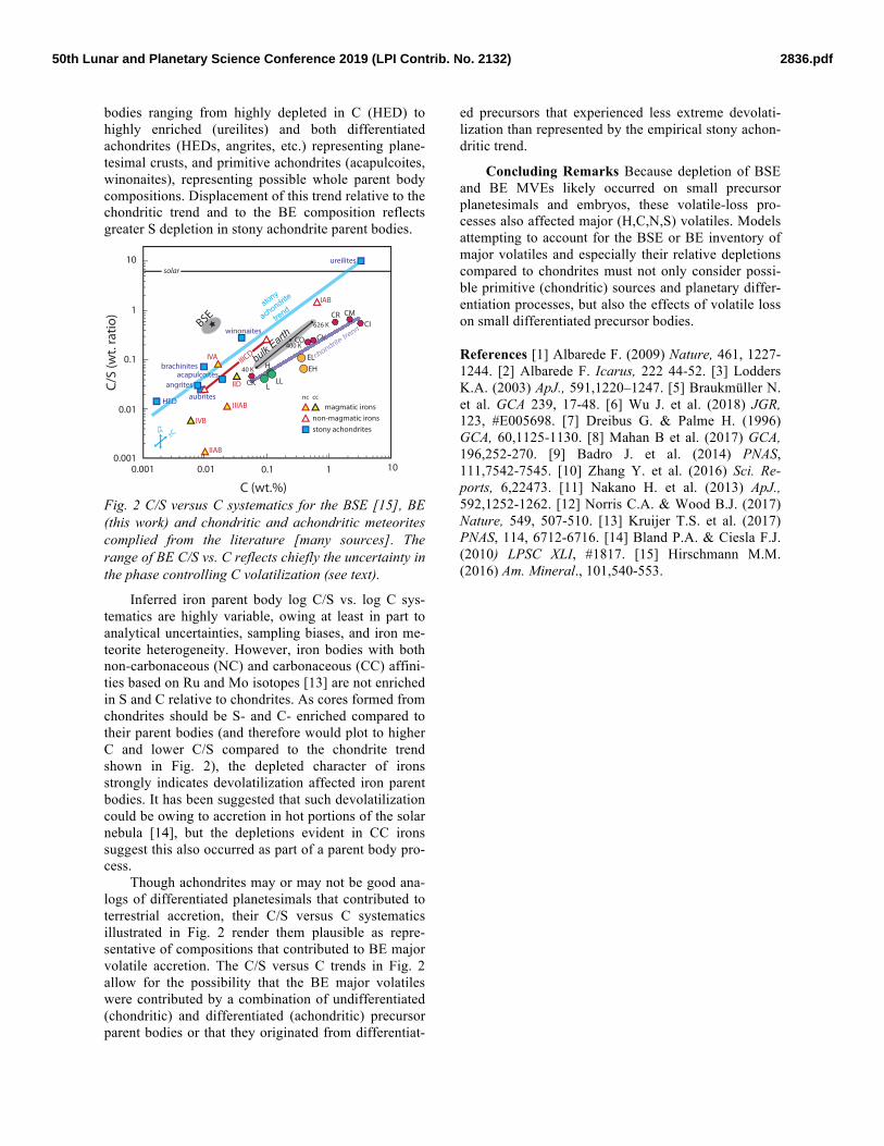
bodies ranging from highly depleted in C (HED) to highly enriched (ureilites) and both differentiated achondrites (HEDs, angrites, etc.) representing plane-tesimal crusts, and primitive achondrites (acapulcoites, winonaites), representing possible whole parent body compositions. Displacement of this trend relative to the chondritic trend and to the BE composition reflects greater S depletion in stony achondrite parent bodies.

LLL

CO CV

CMCI

ELEH

10

1

0.1

0.01

0.0010.001 0.01 0.1 101

C (wt.%)

C/S

(wt.

ratio

)

ureilites

winonaites

HED

acapulcoites

aubrites

IAB

IIAB

IVB

IVA IIICD

IIIAB

BSE

magmatic ironsnon-magmatic ironsstony achondrites

solar

400 K

40 Kbulk E

arth626 K

ccnc

angrites IID

±S

±C

CV

chondrite tre

nd

LL

HED

s

coite

s

tes

stony

achondrite

trend

Hbrachinites

CR

CK

Fig. 2 C/S versus C systematics for the BSE [15], BE (this work) and chondritic and achondritic meteorites complied from the literature [many sources]. The range of BE C/S vs. C reflects chiefly the uncertainty in the phase controlling C volatilization (see text).

Inferred iron parent body log C/S vs. log C sys-tematics are highly variable, owing at least in part to analytical uncertainties, sampling biases, and iron me-teorite heterogeneity. However, iron bodies with both non-carbonaceous (NC) and carbonaceous (CC) affini-ties based on Ru and Mo isotopes [13] are not enriched in S and C relative to chondrites. As cores formed from chondrites should be S- and C- enriched compared to their parent bodies (and therefore would plot to higher C and lower C/S compared to the chondrite trend shown in Fig. 2), the depleted character of irons strongly indicates devolatilization affected iron parent bodies. It has been suggested that such devolatilization could be owing to accretion in hot portions of the solar nebula [14], but the depletions evident in CC irons suggest this also occurred as part of a parent body pro-cess.

Though achondrites may or may not be good ana-logs of differentiated planetesimals that contributed to terrestrial accretion, their C/S versus C systematics illustrated in Fig. 2 render them plausible as repre-sentative of compositions that contributed to BE major volatile accretion. The C/S versus C trends in Fig. 2 allow for the possibility that the BE major volatiles were contributed by a combination of undifferentiated (chondritic) and differentiated (achondritic) precursor parent bodies or that they originated from differentiat-

ed precursors that experienced less extreme devolati-lization than represented by the empirical stony achon-dritic trend.

Concluding Remarks Because depletion of BSE and BE MVEs likely occurred on small precursor planetesimals and embryos, these volatile-loss pro-cesses also affected major (H,C,N,S) volatiles. Models attempting to account for the BSE or BE inventory of major volatiles and especially their relative depletions compared to chondrites must not only consider possi-ble primitive (chondritic) sources and planetary differ-entiation processes, but also the effects of volatile loss on small differentiated precursor bodies. References [1] Albarede F. (2009) Nature, 461, 1227-1244. [2] Albarede F. Icarus, 222 44-52. [3] Lodders K.A. (2003) ApJ., 591,1220–1247. [5] Braukmüller N. et al. GCA 239, 17-48. [6] Wu J. et al. (2018) JGR, 123, #E005698. [7] Dreibus G. & Palme H. (1996) GCA, 60,1125-1130. [8] Mahan B et al. (2017) GCA, 196,252-270. [9] Badro J. et al. (2014) PNAS, 111,7542-7545. [10] Zhang Y. et al. (2016) Sci. Re-ports, 6,22473. [11] Nakano H. et al. (2013) ApJ., 592,1252-1262. [12] Norris C.A. & Wood B.J. (2017) Nature, 549, 507-510. [13] Kruijer T.S. et al. (2017) PNAS, 114, 6712-6716. [14] Bland P.A. & Ciesla F.J. (2010) LPSC XLI, #1817. [15] Hirschmann M.M. (2016) Am. Mineral., 101,540-553.


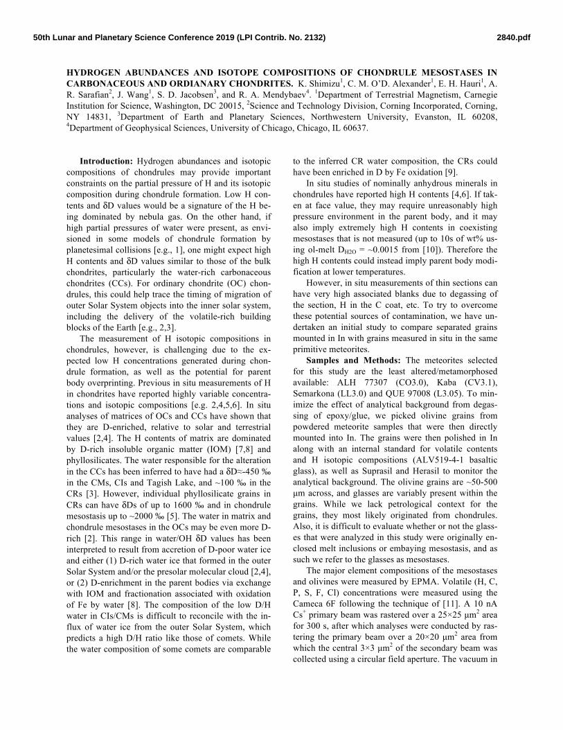
HYDROGEN ABUNDANCES AND ISOTOPE COMPOSITIONS OF CHONDRULE MESOSTASES IN CARBONACEOUS AND ORDIANARY CHONDRITES. K. Shimizu1, C. M. O’D. Alexander1, E. H. Hauri1, A. R. Sarafian2, J. Wang1, S. D. Jacobsen3, and R. A. Mendybaev4. 1Department of Terrestrial Magnetism, Carnegie Institution for Science, Washington, DC 20015, 2Science and Technology Division, Corning Incorporated, Corning, NY 14831, 3Department of Earth and Planetary Sciences, Northwestern University, Evanston, IL 60208, 4Department of Geophysical Sciences, University of Chicago, Chicago, IL 60637.

Introduction: Hydrogen abundances and isotopic

compositions of chondrules may provide important constraints on the partial pressure of H and its isotopic composition during chondrule formation. Low H con-tents and δD values would be a signature of the H be-ing dominated by nebula gas. On the other hand, if high partial pressures of water were present, as envi-sioned in some models of chondrule formation by planetesimal collisions [e.g., 1], one might expect high H contents and δD values similar to those of the bulk chondrites, particularly the water-rich carbonaceous chondrites (CCs). For ordinary chondrite (OC) chon-drules, this could help trace the timing of migration of outer Solar System objects into the inner solar system, including the delivery of the volatile-rich building blocks of the Earth [e.g., 2,3].

The measurement of H isotopic compositions in chondrules, however, is challenging due to the ex-pected low H concentrations generated during chon-drule formation, as well as the potential for parent body overprinting. Previous in situ measurements of H in chondrites have reported highly variable concentra-tions and isotopic compositions [e.g. 2,4,5,6]. In situ analyses of matrices of OCs and CCs have shown that they are D-enriched, relative to solar and terrestrial values [2,4]. The H contents of matrix are dominated by D-rich insoluble organic matter (IOM) [7,8] and phyllosilicates. The water responsible for the alteration in the CCs has been inferred to have had a δD≈-450 ‰ in the CMs, CIs and Tagish Lake, and ~100 ‰ in the CRs [3]. However, individual phyllosilicate grains in CRs can have δDs of up to 1600 ‰ and in chondrule mesostasis up to ~2000 ‰ [5]. The water in matrix and chondrule mesostases in the OCs may be even more D-rich [2]. This range in water/OH δD values has been interpreted to result from accretion of D-poor water ice and either (1) D-rich water ice that formed in the outer Solar System and/or the presolar molecular cloud [2,4], or (2) D-enrichment in the parent bodies via exchange with IOM and fractionation associated with oxidation of Fe by water [8]. The composition of the low D/H water in CIs/CMs is difficult to reconcile with the in-flux of water ice from the outer Solar System, which predicts a high D/H ratio like those of comets. While the water composition of some comets are comparable

to the inferred CR water composition, the CRs could have been enriched in D by Fe oxidation [9].

In situ studies of nominally anhydrous minerals in chondrules have reported high H contents [4,6]. If tak-en at face value, they may require unreasonably high pressure environment in the parent body, and it may also imply extremely high H contents in coexisting mesostases that is not measured (up to 10s of wt% us-ing ol-melt DH2O = ~0.0015 from [10]). Therefore the high H contents could instead imply parent body modi-fication at lower temperatures.

However, in situ measurements of thin sections can have very high associated blanks due to degassing of the section, H in the C coat, etc. To try to overcome these potential sources of contamination, we have un-dertaken an initial study to compare separated grains mounted in In with grains measured in situ in the same primitive meteorites.

Samples and Methods: The meteorites selected for this study are the least altered/metamorphosed available: ALH 77307 (CO3.0), Kaba (CV3.1), Semarkona (LL3.0) and QUE 97008 (L3.05). To min-imize the effect of analytical background from degas-sing of epoxy/glue, we picked olivine grains from powdered meteorite samples that were then directly mounted into In. The grains were then polished in In along with an internal standard for volatile contents and H isotopic compositions (ALV519-4-1 basaltic glass), as well as Suprasil and Herasil to monitor the analytical background. The olivine grains are ~50-500 µm across, and glasses are variably present within the grains. While we lack petrological context for the grains, they most likely originated from chondrules. Also, it is difficult to evaluate whether or not the glass-es that were analyzed in this study were originally en-closed melt inclusions or embaying mesostasis, and as such we refer to the glasses as mesostases.

The major element compositions of the mesostases and olivines were measured by EPMA. Volatile (H, C, P, S, F, Cl) concentrations were measured using the Cameca 6F following the technique of [11]. A 10 nA Cs+ primary beam was rastered over a 25×25 µm2 area for 300 s, after which analyses were conducted by ras-tering the primary beam over a 20×20 µm2 area from which the central 3×3 µm2 of the secondary beam was collected using a circular field aperture. The vacuum in


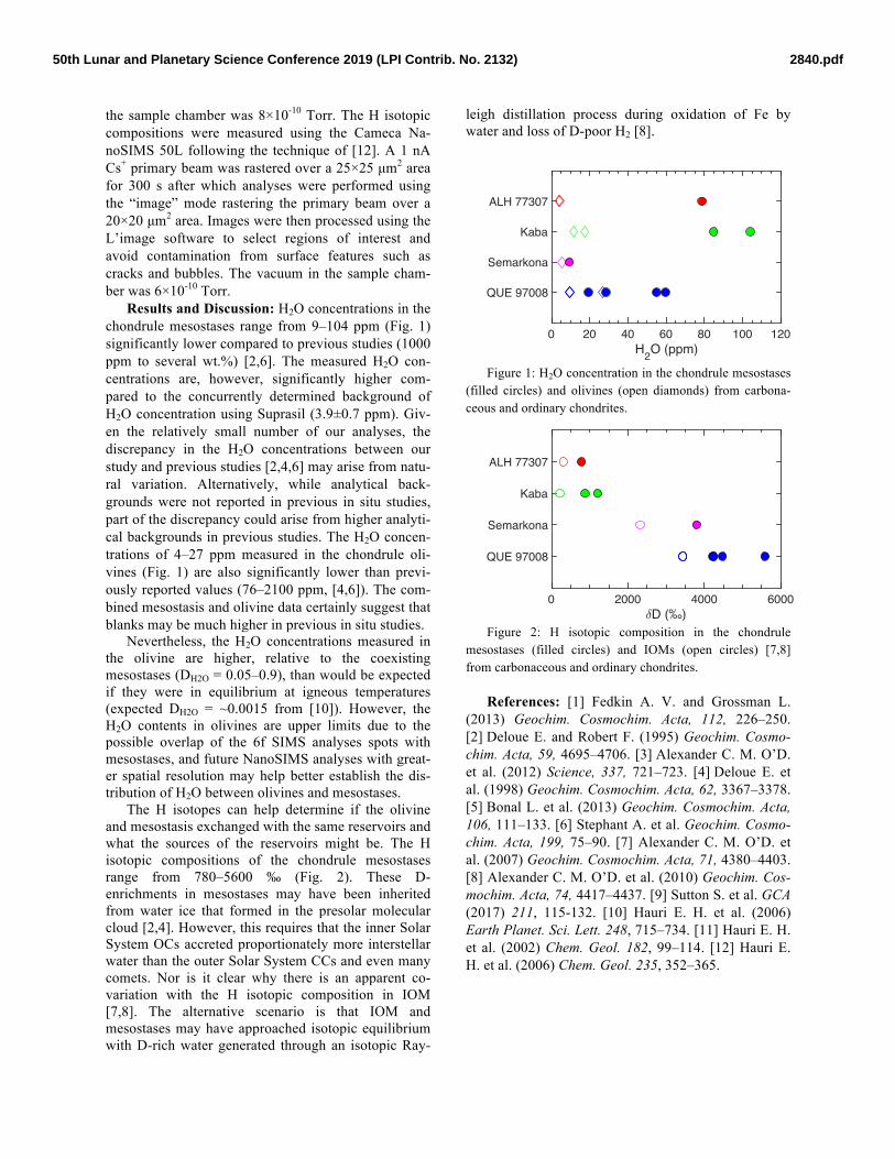
the sample chamber was 8×10-10 Torr. The H isotopic compositions were measured using the Cameca Na-noSIMS 50L following the technique of [12]. A 1 nA Cs+ primary beam was rastered over a 25×25 µm2 area for 300 s after which analyses were performed using the “image” mode rastering the primary beam over a 20×20 µm2 area. Images were then processed using the L’image software to select regions of interest and avoid contamination from surface features such as cracks and bubbles. The vacuum in the sample cham-ber was 6×10-10 Torr.

Results and Discussion: H2O concentrations in the chondrule mesostases range from 9–104 ppm (Fig. 1) significantly lower compared to previous studies (1000 ppm to several wt.%) [2,6]. The measured H2O con-centrations are, however, significantly higher com-pared to the concurrently determined background of H2O concentration using Suprasil (3.9±0.7 ppm). Giv-en the relatively small number of our analyses, the discrepancy in the H2O concentrations between our study and previous studies [2,4,6] may arise from natu-ral variation. Alternatively, while analytical back-grounds were not reported in previous in situ studies, part of the discrepancy could arise from higher analyti-cal backgrounds in previous studies. The H2O concen-trations of 4–27 ppm measured in the chondrule oli-vines (Fig. 1) are also significantly lower than previ-ously reported values (76–2100 ppm, [4,6]). The com-bined mesostasis and olivine data certainly suggest that blanks may be much higher in previous in situ studies.

Nevertheless, the H2O concentrations measured in the olivine are higher, relative to the coexisting mesostases (DH2O = 0.05–0.9), than would be expected if they were in equilibrium at igneous temperatures (expected DH2O = ~0.0015 from [10]). However, the H2O contents in olivines are upper limits due to the possible overlap of the 6f SIMS analyses spots with mesostases, and future NanoSIMS analyses with great-er spatial resolution may help better establish the dis-tribution of H2O between olivines and mesostases.

The H isotopes can help determine if the olivine and mesostasis exchanged with the same reservoirs and what the sources of the reservoirs might be. The H isotopic compositions of the chondrule mesostases range from 780–5600 ‰ (Fig. 2). These D-enrichments in mesostases may have been inherited from water ice that formed in the presolar molecular cloud [2,4]. However, this requires that the inner Solar System OCs accreted proportionately more interstellar water than the outer Solar System CCs and even many comets. Nor is it clear why there is an apparent co-variation with the H isotopic composition in IOM [7,8]. The alternative scenario is that IOM and mesostases may have approached isotopic equilibrium with D-rich water generated through an isotopic Ray-

leigh distillation process during oxidation of Fe by water and loss of D-poor H2 [8].

0 20 40 60 80 100 120H2O (ppm)

QUE 97008

Semarkona

Kaba

ALH 77307

Figure 1: H2O concentration in the chondrule mesostases

(filled circles) and olivines (open diamonds) from carbona-ceous and ordinary chondrites.

0 2000 4000 6000

QUE 97008

Semarkona

Kaba

ALH 77307

Figure 2: H isotopic composition in the chondrule

mesostases (filled circles) and IOMs (open circles) [7,8] from carbonaceous and ordinary chondrites.

References: [1] Fedkin A. V. and Grossman L. (2013) Geochim. Cosmochim. Acta, 112, 226–250. [2] Deloue E. and Robert F. (1995) Geochim. Cosmo-chim. Acta, 59, 4695–4706. [3] Alexander C. M. O’D. et al. (2012) Science, 337, 721–723. [4] Deloue E. et al. (1998) Geochim. Cosmochim. Acta, 62, 3367–3378. [5] Bonal L. et al. (2013) Geochim. Cosmochim. Acta, 106, 111–133. [6] Stephant A. et al. Geochim. Cosmo-chim. Acta, 199, 75–90. [7] Alexander C. M. O’D. et al. (2007) Geochim. Cosmochim. Acta, 71, 4380–4403. [8] Alexander C. M. O’D. et al. (2010) Geochim. Cos-mochim. Acta, 74, 4417–4437. [9] Sutton S. et al. GCA (2017) 211, 115-132. [10] Hauri E. H. et al. (2006) Earth Planet. Sci. Lett. 248, 715–734. [11] Hauri E. H. et al. (2002) Chem. Geol. 182, 99–114. [12] Hauri E. H. et al. (2006) Chem. Geol. 235, 352–365.


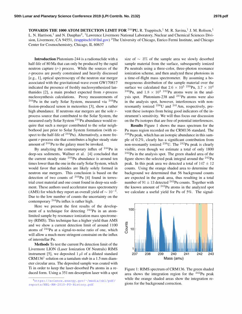
TOWARDS THE 1000 ATOM DETECTION LIMIT FOR 244PU. R. Trappitsch,1 M. R. Savina,1 J. M. Rolison,1

L. N. Harrison,1 and N. Dauphas2, 1Lawrence Livermore National Laboratory, Nuclear and Chemical Sciences Divi-sion, Livermore, CA 94551, ([email protected]) 2The University of Chicago, Enrico Fermi Institute, and ChicagoCenter for Cosmochemistry, Chicago, IL 60637

Introduction Plutonium-244 is a radionuclide with ahalf-life of 80 Ma that can only be produced by the rapidneutron capture (r-) process. While the sources of ther-process are poorly constrained and heavily discussed[e.g., 1], optical spectroscopy of the neutron star mergerassociated with the gravitational-wave event GW170817indicated the presence of freshly nucleosynthesized lan-thanides [2], a main product expected from r-processnucleosynthesis calculations. Proxy measurements of244Pu in the early Solar System, measured via 244Pufission-produced xenon in meteorites [3], show a ratherhigh abundance. If neutrons star mergers are the sole r-process source that contributed to the Solar System, themeasured early Solar System 244Pu abundance would re-quire that such a merger contributed to the solar neigh-borhood just prior to Solar System formation (with re-spect to the half-life of 244Pu). Alternatively, a more fre-quent r-process site that contributes a higher steady stateamount of 244Pu to the galaxy must be invoked.

By analyzing the contemporary influx of 244Pu indeep-sea sediments, Wallner et al. [4] concluded thatthe current steady state 244Pu abundance is around tentimes lower than the one in the early Solar System, whichwould favor that actinides are likely solely formed inneutron star mergers. This conclusion is based on thedetection of two counts of 244Pu [4] found in terres-trial crust material and one count found in deep-sea sedi-ment. These authors used accelerator mass spectrometry(AMS) for which they report an overall yield of ∼ 10−4.Due to the low number of counts the uncertainty on thecontemporary 244Pu influx is rather high.

Here we present the first results of the develop-ment of a technique for detecting 244Pu in an atom-limited sample by resonance ionization mass spectrome-try (RIMS). This technique has a higher yield than AMSand we show a current detection limit of around 1100atoms of 244Pu at a signal-to-noise ratio of one, whichwill allow a much more stringent constraint on the influxof interstellar Pu.

Methods To test the current Pu detection limit of theLivermore LION (Laser Ionization Of Neutrals) RIMSinstrument [5], we deposited 1µl of a diluted standardCRM1361 solution on a tantalum stub in a 1.5 mm diam-eter circular area. The deposited sample was coated withTi in order to keep the laser-desorbed Pu atoms in a re-duced form. Using a 351 nm desorption laser with a spot

1https://science.energy.gov/˜/media/nbl/pdf/reports/NBL-RM-2010-PU-History.pdf

size of ∼ 3% of the sample area we slowly desorbedsample material from the surface, subsequently ionizedPu neutrals using a three-color, three-photon resonanceionization scheme, and then analyzed these photoions ina time-of-flight mass spectrometer. By assuming a ho-mogeneous distribution of the sample material over thesurface we calculated that 2.6 × 105 239Pu, 3.7 × 104240Pu, and 1.8 × 103 242Pu atoms were in the anal-ysis spot. Plutonium-238 and 241Pu atoms were alsoin the analysis spot, however, interferences with non-resonantly ionized 238U and 241Am, respectively, pre-vent these isotopes from being good indicators of the in-strument’s sensitivity. We will thus focus our discussionon the Pu isotopes that are free of potential interferences.

Results Figure 1 shows the mass spectrum for thePu mass region recorded on the CRM136 standard. The238Pu peak, which has an isotopic abundance in this sam-ple of 0.2%, clearly has a significant contribution fromnon-resonantly ionized 238U. The 242Pu peak is clearlyvisible, even though we estimate a total of only 1800242Pu in the analysis spot. The green shaded area of thefigure shows the selected peak integral around the 242Pupeak. In this peak area we detected a total of 147 ± 12counts. Using the orange shaded area to determine thebackground we determined that 56 background countsare expected in the peak area, thus resulting in a totalnumber of 91± 13 detected 242Pu counts. Together withthe known amount of 242Pu atoms in the analyzed spotwe calculate a useful yield for Pu of 5%. The signal-

Cou

nts

1

10

100

Mass (amu)237 238 239 240 241 242 243

Figure 1: RIMS spectrum of CRM136. The green shadedarea shows the integration region for the 242Pu peakwhile the orange shaded areas show the integration re-gions for the background correction.



https://science.energy.gov/~/media/nbl/pdf/reports/NBL-RM-2010-PU-History.pdf

https://science.energy.gov/~/media/nbl/pdf/reports/NBL-RM-2010-PU-History.pdf

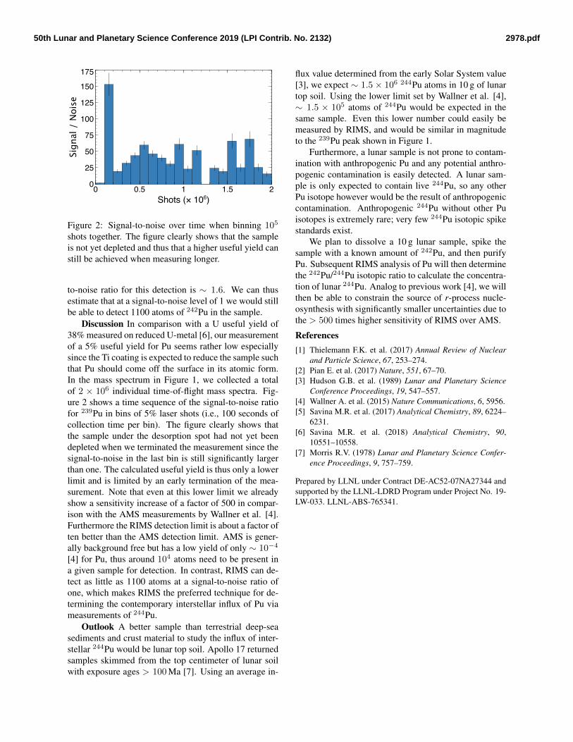
Sign

al /

Noi

se

0

25

50

75

100

125

150

175

Shots (× 106)0 0.5 1 1.5 2

Figure 2: Signal-to-noise over time when binning 105

shots together. The figure clearly shows that the sampleis not yet depleted and thus that a higher useful yield canstill be achieved when measuring longer.

to-noise ratio for this detection is ∼ 1.6. We can thusestimate that at a signal-to-noise level of 1 we would stillbe able to detect 1100 atoms of 242Pu in the sample.

Discussion In comparison with a U useful yield of38% measured on reduced U-metal [6], our measurementof a 5% useful yield for Pu seems rather low especiallysince the Ti coating is expected to reduce the sample suchthat Pu should come off the surface in its atomic form.In the mass spectrum in Figure 1, we collected a totalof 2 × 106 individual time-of-flight mass spectra. Fig-ure 2 shows a time sequence of the signal-to-noise ratiofor 239Pu in bins of 5% laser shots (i.e., 100 seconds ofcollection time per bin). The figure clearly shows thatthe sample under the desorption spot had not yet beendepleted when we terminated the measurement since thesignal-to-noise in the last bin is still significantly largerthan one. The calculated useful yield is thus only a lowerlimit and is limited by an early termination of the mea-surement. Note that even at this lower limit we alreadyshow a sensitivity increase of a factor of 500 in compar-ison with the AMS measurements by Wallner et al. [4].Furthermore the RIMS detection limit is about a factor often better than the AMS detection limit. AMS is gener-ally background free but has a low yield of only ∼ 10−4

[4] for Pu, thus around 104 atoms need to be present ina given sample for detection. In contrast, RIMS can de-tect as little as 1100 atoms at a signal-to-noise ratio ofone, which makes RIMS the preferred technique for de-termining the contemporary interstellar influx of Pu viameasurements of 244Pu.

Outlook A better sample than terrestrial deep-seasediments and crust material to study the influx of inter-stellar 244Pu would be lunar top soil. Apollo 17 returnedsamples skimmed from the top centimeter of lunar soilwith exposure ages > 100Ma [7]. Using an average in-

flux value determined from the early Solar System value[3], we expect ∼ 1.5× 106 244Pu atoms in 10 g of lunartop soil. Using the lower limit set by Wallner et al. [4],∼ 1.5 × 105 atoms of 244Pu would be expected in thesame sample. Even this lower number could easily bemeasured by RIMS, and would be similar in magnitudeto the 239Pu peak shown in Figure 1.

Furthermore, a lunar sample is not prone to contam-ination with anthropogenic Pu and any potential anthro-pogenic contamination is easily detected. A lunar sam-ple is only expected to contain live 244Pu, so any otherPu isotope however would be the result of anthropogeniccontamination. Anthropogenic 244Pu without other Puisotopes is extremely rare; very few 244Pu isotopic spikestandards exist.

We plan to dissolve a 10 g lunar sample, spike thesample with a known amount of 242Pu, and then purifyPu. Subsequent RIMS analysis of Pu will then determinethe 242Pu/244Pu isotopic ratio to calculate the concentra-tion of lunar 244Pu. Analog to previous work [4], we willthen be able to constrain the source of r-process nucle-osynthesis with significantly smaller uncertainties due tothe > 500 times higher sensitivity of RIMS over AMS.

References[1] Thielemann F.K. et al. (2017) Annual Review of Nuclear

and Particle Science, 67, 253–274.[2] Pian E. et al. (2017) Nature, 551, 67–70.[3] Hudson G.B. et al. (1989) Lunar and Planetary Science

Conference Proceedings, 19, 547–557.[4] Wallner A. et al. (2015) Nature Communications, 6, 5956.[5] Savina M.R. et al. (2017) Analytical Chemistry, 89, 6224–

6231.[6] Savina M.R. et al. (2018) Analytical Chemistry, 90,

10551–10558.[7] Morris R.V. (1978) Lunar and Planetary Science Confer-

ence Proceedings, 9, 757–759.

Prepared by LLNL under Contract DE-AC52-07NA27344 andsupported by the LLNL-LDRD Program under Project No. 19-LW-033. LLNL-ABS-765341.


PROGRESS REPORT ON Lu-Hf MEASUREMENTS OF SINGLE ZIRCON GRAINS AT THE UNIVERSITY OF CHICAGO. X.C. Chen1, N. Dauphas1, K.D. McKeegan2, M. Barboni3, B. Schoene4, P. Boehnke1, 1Origins Lab, Department of the Geophysical Sciences, and Enrico Fermi Institute, The University of Chi-cago, Chicago, IL ([email protected]), 2Department of Earth, Planetary and Space Sciences, University of California, Los Angeles, Los Angeles, CA, 3School of Earth and Space Exploration, Arizona State University, Tempe, AZ, 4Department of Geosciences, Princeton University, Princeton, NJ.

Introduction: Previous studies coupled U-Pb and Lu-Hf isotopic

analyses of single lunar zircon grains to derive a mini-mum age for the isolation of the KREEP reservoir; the very last residual melt produced by crystallization of the the Lunar Magma Ocean. The result of those analyses gives an early age of ~4.51 Ga [1,2]. This minimum age for the differentiation of the lunar crust is mostly based on four zircons with the least radiogenic Hf isotopic compositions. The age of KREEP from zircon analyses is ~120 to 150 Myr older than estimates based on Sm-Nd and Pb-Pb isochrons in ferroan anorthosites [3] and dating of Mg suite lunar crustal rocks [4].

There are several potential difficulties associated with the zircon approach. One is that most lunar zircons are small so that the amount of Hf available for isotopic analysis is small, which limits the precision attainable. Another is that it relies on extreme unradiogenic iso-topic analyses of zircons so measurement accuracy of every single data point is critical. Previous lunar zircon εHf results were reported at 1 to 4 epsilon uncertainty (2σ). Higher precision and high-accuracy measure-ments are needed to provide more robust constraints on the minimum age of formation of the Moon and crystal-lization of the LMO. Here, we report our progress to implement the Lu-Hf technique at the University of Chi-cago for measurements of single zircon grains. We use an ion-exchange procedure to purify Zr and Hf from the interfering Yb and Lu elements [e.g. 5-8] in the diges-tion solutions of individual lunar zircons retrieved after U-Pb chemistry. This can potentially give smaller er-rors than applying a peak-stripping method [2]. It also allows us to recover the purified Zr for future isotopic studies.

Method and Discussion: A two-stage procedure (following the modified pro-cedure of [7] and [9]) was developed for separating Zr and Hf. In the first step, TODGA resin is used to collect a zirconium-hafnium cut following the titanium separa-tion methods [10]. In the second step, Ln-Spec resin is used to further separate Zr and Hf. Elution tests were done using a multi-element standard solution containing Zr, Hf and 24 other elements (including all the HFSEs and REEs). The Hf procedural blank was below detec-tion limit and the yield was >80%. We also performed chemical separations on the solutions retrieved after U-

Pb chemistry of some zircon standards (AS3, 91500, and Mudtank).

The Hf isotope analyses were performed on a Nep-tune Plus multi-collector inductively coupled plasma mass spectrometer (ThermoFinnigan) connected to an Aridus II desolvating nebulizer. Matrix purification drastically decreases interferences and permits the use of high-transmission Jet sample and X-skimmer cones, which enhances the sensitivity of the instrument. The purified Hf fractions were dissolved in 0.3 M HNO3 + 0.07 M HF. The achieved sensitivity was 1.5 V/10 ppb for 177Hf (18.60%) at a sample uptake rate of ∼150 µL/min. For isotope ratio measurements of purified Hf fractions, the isotopes 174Hf, 176Hf, 177Hf, 178Hf, 179Hf, and 180Hf as well as 172Yb, 175Lu, and 184W were moni-tored with static mode on nine Faraday cups. We found that the interferences of Yb, Lu, and W on Hf isotopes are negligible due to efficient separation of Hf in the ion exchange chemistry. Each measurement took 30 cycles with each cycle taking 8.389 seconds. Individual sam-ple measurements were bracketed by the analysis of JMC-Hf 475 standard solutions whose concentrations are adjusted to match those of the samples that they bracket. The mass bias factor was calculated by nor-malizing the measured 179Hf/177Hf to 0.7325 [11] with an exponential law. The Hf isotopic ratios of all sam-ples corrected for mass bias were determined relative to the bracketing standard runs and are expressed as ε174,176,178,180Hf, which are the deviations of the 174,176,178,180Hf/177Hf ratios from the standard solution (JMC-Hf 475) in parts per ten thousand. These eHf ra-tios were further normalized to reference values of 180Hf/177Hf = 1.886666, 178Hf/177Hf = 1.467168, and 176Hf/177Hf = 0.282160 for Johnson Matthey Company (JMC)-Hf 475 [6] to allow comparison with literature values. The external reproducibilities were evaluated by repeat analyses of the standard bracketing by itself.

The Hf isotopic compositions of lunar zircons are corrected for radiogenic 176Hf ingrowth by combining TIMS high-precision U-Pb crystallization ages and Lu/Hf ratios in those samples. Each data is also cor-rected for neutron capture effects [2,12,13].

In Figure 1, we show the theoretically achievable precisions on Hf isotopes when measuring Hf isotopic composition bracketing with 1 ml JMC-Hf 475 standard


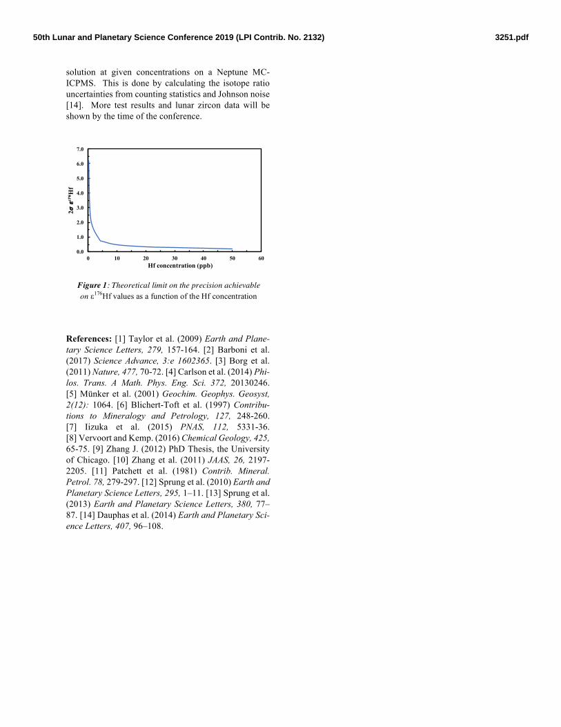
solution at given concentrations on a Neptune MC-ICPMS. This is done by calculating the isotope ratio uncertainties from counting statistics and Johnson noise [14]. More test results and lunar zircon data will be shown by the time of the conference.

References: [1] Taylor et al. (2009) Earth and Plane-tary Science Letters, 279, 157-164. [2] Barboni et al. (2017) Science Advance, 3:e 1602365. [3] Borg et al. (2011) Nature, 477, 70-72. [4] Carlson et al. (2014) Phi-los. Trans. A Math. Phys. Eng. Sci. 372, 20130246. [5] Münker et al. (2001) Geochim. Geophys. Geosyst, 2(12): 1064. [6] Blichert-Toft et al. (1997) Contribu-tions to Mineralogy and Petrology, 127, 248-260. [7] Iizuka et al. (2015) PNAS, 112, 5331-36. [8] Vervoort and Kemp. (2016) Chemical Geology, 425, 65-75. [9] Zhang J. (2012) PhD Thesis, the University of Chicago. [10] Zhang et al. (2011) JAAS, 26, 2197-2205. [11] Patchett et al. (1981) Contrib. Mineral. Petrol. 78, 279-297. [12] Sprung et al. (2010) Earth and Planetary Science Letters, 295, 1–11. [13] Sprung et al. (2013) Earth and Planetary Science Letters, 380, 77–87. [14] Dauphas et al. (2014) Earth and Planetary Sci-ence Letters, 407, 96–108.

0.0

1.0

2.0

3.0

4.0

5.0

6.0

7.0

0 10 20 30 40 50 60

2!" ¹⁷

⁶Hf

Hf concentration (ppb)

Figure 1: Theoretical limit on the precision achievable on ε176Hf values as a function of the Hf concentration


Documents

A NEW MARTIAN PALAEOPRESSURE CONSTRAINT