Embed Size (px)
Citation preview

New Filtering for the cumulative Constraintin the Context of Non-Overlapping Rectangles
Nicolas Beldiceanu1, Mats Carlsson2, and Emmanuel Poder1
1 Ecole des Mines de Nantes, LINA UMR CNRS 6241, FR-44307 Nantes, France{Nicolas.Beldiceanu,Emmanuel.Poder}@emn.fr
2 SICS, P.O. Box 1263, SE-164 29 Kista, [email protected]
Abstract. This paper describes new filtering methods for the cumulative con-straint. The first method introduces bounds for the so called longest cumula-tive hole problem and shows how to use these bounds in the context of thenon-overlapping constraint. The second method introduces balancing knapsackconstraints which relate the total height of the tasks that end at a specific time-point with the total height of the tasks that start at the same time-point. Exper-iments on tight rectangle packing problems show that these methods drasticallyreduce both the time and the number of backtracks for finding all solutions aswell as for finding the first solution. For example, we found without backtrackingall solutions to 66 perfect square instances of order 23-25 and sizes ranging from332 × 332 to 661 × 661.
1 Introduction
The utility of cumulative constraints in the context of non-overlapping rectangles hasbeen advocated for 15 years in the context of constraint programming [1]. The twomain reasons for this utility are: first, it allows to come up with necessary conditions fornon-overlapping which reuse classical filtering algorithms for cumulative like task in-tervals [2, 3] and compulsory parts [4]; second, it reduces in practice the combinatorialaspect by dividing by a factor of two the number of decision variables of the problem.1
More recently, cumulative constraints have been used by OR people [7] in the contextof rectangle packing problems for the reasons we have just mentioned. Knapsack con-straints were also used, by both OR [8, 7] and CP [9] people, to solve the subset-sumproblem in the context of scheduling and packing.
In the context of tight rectangle placement problems one can observe that standardfiltering methods for the cumulative constraint are in fact rather weak. A first reason isthat they do not explicitly completely integrate the slack (i.e., the difference between theavailable place and the total area of the rectangles to place) within the filtering process.A second reason is that they relax too much the cumulative constraint by allowing tosplit the tasks in small squares of size one. Based on these observations, we decided to
1 Experiments have shown [1, 5] that, once all coordinates of the rectangles in one dimensionare fixed, it is usually straightforward to extend the partial solution to a full solution even ifthere exist examples [6] where this is not possible at all.

develop new filtering methods that consider the slack and/or the fact that tasks shouldnot be split in too many small pieces.
The paper is organized as follows. Section 2 recalls the definitions of the cumulative
and the non-overlapping constraints. Section 3 introduces the longest cumulative holeproblem, shows its use in the context of the cumulative constraint, and provides boundsfor this problem. Section 4 presents a new knapsack model of the cumulative con-straint which considers the available slack. Section 5 evaluates the contribution of thetwo methods on two types of tight placement problems. Finally, Section 6 concludes.
2 Background
The cumulative constraint was introduced in [1] in order to model scheduling problemswhere one has to deal with a resource of limited capacity. It has the following definition:
cumulative(T, L)
where for a task t ∈ T , t.s, t.d and t.h denote respectively its start, duration and height.They all correspond to integer variables2, while L is a non-negative integer correspond-ing to the capacity of the resource. The constraint holds if the following condition istrue:
∀i ∈ N,∑
t|t.s≤i≤t.s+t.d−1
t.h ≤ L
In the context of a cumulative constraint, the compulsory part [4] of a task t is theintersection of all feasible instances of t. It can be computed by making the intersectionbetween the task positioned at its earliest start and the task positioned at its latest start.Then the compulsory part profile is the aggregation of all compulsory parts of the differ-ent tasks of a cumulative constraint. When all tasks that have a non-empty compulsorypart are completely fixed, the compulsory part profile is simply called the cumulativeprofile.
The diffn constraint was introduced in [10] in order to handle multi-dimensionalplacement problems. It has the following definition:
diffn(B)
where for a box b ∈ B, b.ok and b.sk (0 ≤ k ≤ n − 1) are integer variables thatrespectively denote the origin and size of b in dimension k. The constraint holds when,for each pair of boxes b, b′, there exist at least one dimension k where their projectionsdo not overlap.
∀b, b′ ∈ B (b 6= b′), ∃k ∈ [0, n− 1] | b.ok ≥ b′.ok + b′.sk ∨ b′.ok ≥ b.ok + b.sk
2 An integer variable V ranges over a finite set of integers denoted by D(V ). The extremalvalues in D(V ) are denoted by V and V .
2

In the context of this paper we focus on the two-dimensional case (n = 2), andassume that all the rectangle sizes are fixed. However note that most of the results ofthis paper can be used when we have more than two dimensions, as it is actually thecase for our current implementation.
3 The Longest Cumulative Hole Problem
This section first introduces the longest cumulative hole problem and then shows how itcan be used in the context of a non-overlapping constraint. Finally, it provides differentways for evaluating an upper bound of the longest cumulative hole.
3.1 Defining the Longest Cumulative Hole
Given a cumulative(T, L) constraint that involves a set of tasks T and a resourcelimit L, let σ denote the difference between the available space and the needed space(i.e., σ = (maxt∈T (t.s + t.d) − mint∈T (t.s)) · L −
∑
t∈T t.d · t.h). Now, given aninteger ε ∈ [1, L] and the subset of tasks T ′ of T for which the resource consumptionis at most ε, the longest hole problem3 is to find the largest integer lmax ε
σ(T ′) such thatthere exist a cumulative placement of maximum height ε involving a subset of tasks ofT ′ where, on one interval [i, i + lmax ε
σ(T ′) − 1] of the cumulative profile, the area ofthe empty space does not exceed σ.4
Example 1. First, consider seven tasks of respective size 11 × 11, 9 × 9, 8 × 8, 7 × 7, 6 × 6,4× 4, 2× 2. Part (A) of Figure 1 provides a cumulative profile corresponding to the longest holeproblem according to ε = 11 and σ = 0. The longest hole lmax 11
0 ({11 × 11, 9 × 9, 8 × 8, 7 ×7, 6 × 6, 4 × 4, 2 × 2}) = 17 since:
– The task 8 × 8 can not contribute since a gap of 3 cannot be filled by the unique candidatethe task 2 × 2.
– The task 6 × 6 can also not contribute since a gap of 5 cannot be completely filled by thecandidates 4 × 4 and 2 × 2.
Second, consider a task of size 3 × 2. Part (B) of Figure 1 provides a cumulative profile cor-responding to the longest hole problem according to ε = 11 and σ = 20. The longest holelmax 11
20({3 × 2}) = 2.
Note that when the gap ε is equal to the resource capacity L, the problem of checkingwhether or not a cumulative constraint has a solution coincides with the longest holeproblem so the longest hole problem is clearly NP-hard. Consequently, our goal is tofind upper bounds for the longest hole problem as well as easy cases which can besolved in polynomial time.
3 A related problem when the slack σ is equal to 0 in the context of rectangles non-overlapping(but not in the context of a cumulative constraint) is called the length of the longest flat surfacein http://www.stetson.edu/%7Eefriedma/mathmagic/1099.html.
4 When the set of tasks T is empty we have that lmax ε
σ(T ) = bσ
εc.
3

17
(B)(A)
2
epsil
on=1
1
epsil
on=1
1
���������������������������� ����������
������������������������������������ !!"""###
$$%%&&&'''
1
4
768
2
911
Fig. 1. Two examples for illustrating the longest hole problem
3.2 Using the Longest Cumulative Hole for FilteringThe main advantage of the longest cumulative hole problem is that it can be used inquite a number of different ways in the context of a two-dimensional non-overlappingconstraint, where the slack σ is the difference between the available and the neededspace:
– First, as depicted by Part (A) of Figure 2, it can be used for making an initial prun-ing of the origin coordinates of the rectangles in order to avoid creating too smallholes that cannot be filled enough, with respect to the slack σ, between the borderof a rectangle R1 and the border of the placement space. For instance, Part (A)illustrates the fact that if, for a given distance ε ∈ N between the lower borderof a rectangle to place and the lower border of the placement space, the quantitylmax ε
σ(R) is strictly less than the width of R1, then R1 cannot start at the corre-sponding position. R corresponds to the set of rectangles for which the height doesnot exceed ε (i.e., the rectangles that can fit within the gap). Finally, doing an initialpruning of the origins of the rectangles is important for the knapsack constraintsthat will be presented in the next section.
– Second, while fixing both origin coordinates of a rectangle R1 during the search, itcan also be used to check that the vis-a-vis between R1 and each rectangle that isalready completely fixed5 can be filled enough with respect to σ. This is illustratedby Part (B) of Figure 2.
– Finally, it can also be directly used within the two cumulative constraints, whichare well-known necessary conditions for a non-overlapping constraint. For this pur-pose, consider the highest peak of the compulsory part profile that does not reachthe resource capacity (i.e., the difference between the resource capacity and theheight of the peak is equal to a strictly positive integer ε). Again, we can use thelongest cumulative hole problem in order to check that we can fill enough the gapon top of the highest peak. This is illustrated by Part (C) of Figure 2.
3.3 Evaluating the Longest Cumulative HoleThis section shows how to evaluate an upper bound of lmax ε
σ(T ). It assumes that wealready know:
5 Two fixed rectangles have a vis-a-vis if and only if (1) they intersect in one dimension, and(2) if there is a non-empty gap between them in the other dimension.
4

()(()(()(()(()(()(*)**)**)**)**)**)*+,
-)-.//////000000
1)11)11)11)11)11)12)22)22)22)22)22)23344
(C)(B)(A)
lmax s0
lmax
epsil
on
peakheighest
R1
R2
R1
d=1
d=0
d=1
d=0
d=1
d=0
with dimension 0cumulative profile associated
lmax
<s0
fill e
noug
h on
top
of h
ighe
st p
eak
infe
asib
le s
ince
can
not
cumulative profile of compulsoryparts in dimension 0
lmax
<s0
betw
een
R1 a
nd R
2in
feas
ible
vis−
à−vis
cumulative profile associatedwith dimension 0
lmax
<l0
for t
he o
rigin
of R
1in
feas
ible
val
ue
with dimension 0cumulative profile associated
)(s
ince
lmax
epsil
on
(sin
ce
s0
)
(sin
ce) l0
epsil
on
Fig. 2. Three ways of using the longest cumulative hole for filtering a two-dimensionalnon-overlapping constraint.
– An upper bound of lmax eσ(T ) for all non-negative integers e that are strictly less
than ε.– An upper bound of lmax e
σ(T \ {t}) for all non-negative integers e that are strictlyless than ε and for all t ∈ T for which t.h ≤ ε.6 This quantity will be used forchecking what can be put on top of a task t without reusing t.
We first present three rules that simplify the problem by removing some tasks, onerule that reduces the length of some tasks7, and a rule that computes an exact valueof lmax e
σ(T ) when a specific condition on the heights of the tasks holds. Finally, wepresent two upper bounds of lmax e
σ(T ) and show that they are incomparable. In thefollowing, a task t of length t.d and height t.h will be denoted by t.d × t.h.
Simplification 1. Let t be a task of T such that t.h > ε. We have that lmax εσ(T ) =
lmaxεσ(T \ {t}).
Proof. By definition of the longest hole problem, a task of height strictly greater than ε cannotbe used.
Example 2. Consider the set of tasks T = {2 × 2, 4 × 4, 6 × 6} and assume that we want tocompute lmax 1
3(T ). Using Simplification 1, we have that lmax 13(T ) = lmax 1
3(∅), which meansthat we can only use the slack of 3 to cover a gap of height 1. Consequently, lmax 1
3(T ) = 3.
Simplification 2. Let Tε denote the set of tasks of T for which the heights are equalto ε. We have that lmax ε
σ(T ) =∑
t∈Tεt.d + lmax ε
σ(T \ Tε).
Proof. Since the tasks of Tε completely fill the height ε, they can be considered separately.
Example 3. Consider the set of tasks T = {2 × 2, 4 × 4, 6 × 6} and assume that we want tocompute lmax 6
0(T ). Using Simplification 2, we have that lmax 60(T ) = 6+ lmax6
0(T \{6×6}).
6 If we don’t want to explicitly evaluate an upper bound of lmax e
σ(T \ {t}), we can take advan-tage of the fact that lmax e
σ(T ) is an upper bound of lmax e
σ(T \ {t}).7 If, as we will see later, a task cannot contribute on its full length to the longest cumulative hole.
5

Simplification 3. Let t be a task of T such that t.h < ε and lmax ε−t.hσ (T \ {t}) = 0.
We have that lmax εσ(T ) = lmax ε
σ(T \ {t}).
Proof. When lmax ε−t.hσ (T \ {t}) is equal to 0, this means that no gap of height ε − t.h can be
filled by the tasks of T \ {t} without creating an empty space greater than the slack σ. Conse-quently, if we use task t, we cannot fill enough any gap on top of task t.
Example 4. Consider the set of tasks T = {2 × 2, 3 × 3} and assume that we want to computelmax 3
0(T ). Assume that we already know that lmax 10(T \ {2 × 2}) = 0. Then, we have that
lmax 30(T ) = lmax 3
0(T \ {2× 2}). In other words, we can eliminate task 2× 2, since we cannotcover any gap of height 1 on top of task 2 × 2.
Shrinking 1. Consider a task t of T such that t.h < ε, t.d > lmax ε−t.hσ (T \ {t}) and
lmax ε−t.hσ (T \ {t}) > 0. We have that lmax ε
σ(T ) ≤ lmax εσ(T \ {t} ∪ {lmax ε−t.h
σ (T \{t}) × t.h}).
Proof. Similar to Simplification 3. We have an inequality since reducing the lengths of more thantwo disjunctive tasks (i.e., two tasks for which the total height is strictly greater than ε) can leadto an overestimation of lmax ε
σ(T ). This stems from the fact that at most two disjunctive taskscan be reduced (and the other disjunctive tasks have to be discarded since they would have to becompletely included within the interval corresponding to the longest cumulative hole).
Example 5. Consider the set of tasks T = {2 × 2, 4 × 4, 6 × 6} and assume that we want tocompute lmax 6
0(T ). Suppose we already know that lmax 20(T \ {4 × 4}) = 2. Then we have
that lmax 60(T ) = lmax 6
0((T \ {4 × 4}) ∪ {2 × 4}). In other words, the length of task 4 × 4is reduced to 2 (i.e., its maximum intersection in time with the longest cumulative hole cannotexceed 2) since, for a gap of 2, we can cover at most a length of 2 without exceeding the slackσ = 0.
In the following, all simplification and shrinking rules previously presented are sys-tematically tried before applying the next rule and before evaluating any upper bound.
Termination rule. Given a set of tasks T = {t1.d× t1.h, t2.d× t2.h, . . . , tn.d× tn.h}such that ti.h ≥ ti+1.h and ti.h = ti+1.h ⇒ ti.d ≥ ti+1.d (1 ≤ i < n), let Tdisj ={t1.d×t1.h, t2.d×t2.h, . . . , tndisj .d×, tndisj .h}, where ndisj is the largest integer thatsatisfies ndisj = 1 or tndisj−1.h + tndisj .h > ε, be the non-empty subset of disjunctivetasks of T . If the total height of the tasks in T \ Tdisj plus the maximum height ofthe tasks in Tdisj (i.e., t1.h) is at most ε, then the quantity lmax ε
σ(T ) can be directlyevaluated by using the construction depicted by Figure 3.8
The intuition of the first upper bound is to consider the total area of the tasks as wellas the slack. However, to get a sharper bound we take into account the fact that at mosttwo disjunctive tasks can partially overlap a given interval.
8 Assuming that the tasks were sorted, a direct algorithm implementing this construction has thecomplexity of O(n) where n is the number of tasks.
6
5657
8689:6::6:;;<6<=>6>?@6@AB6BCD6DD6DEEF6FGH6HI
J6JK6KL6LL6LM6MM6M
N6NO6OP6PP6PQQR6RS6ST6TUV6VV6VWWX6XX6XY6YY6Y Z6ZZ6Z[6[[6[\6\\6\]6]]6]^6^_6_`6`a6a
b6bcd6dd6deef6fg
lmax=8
epsilon=10
65
321
4
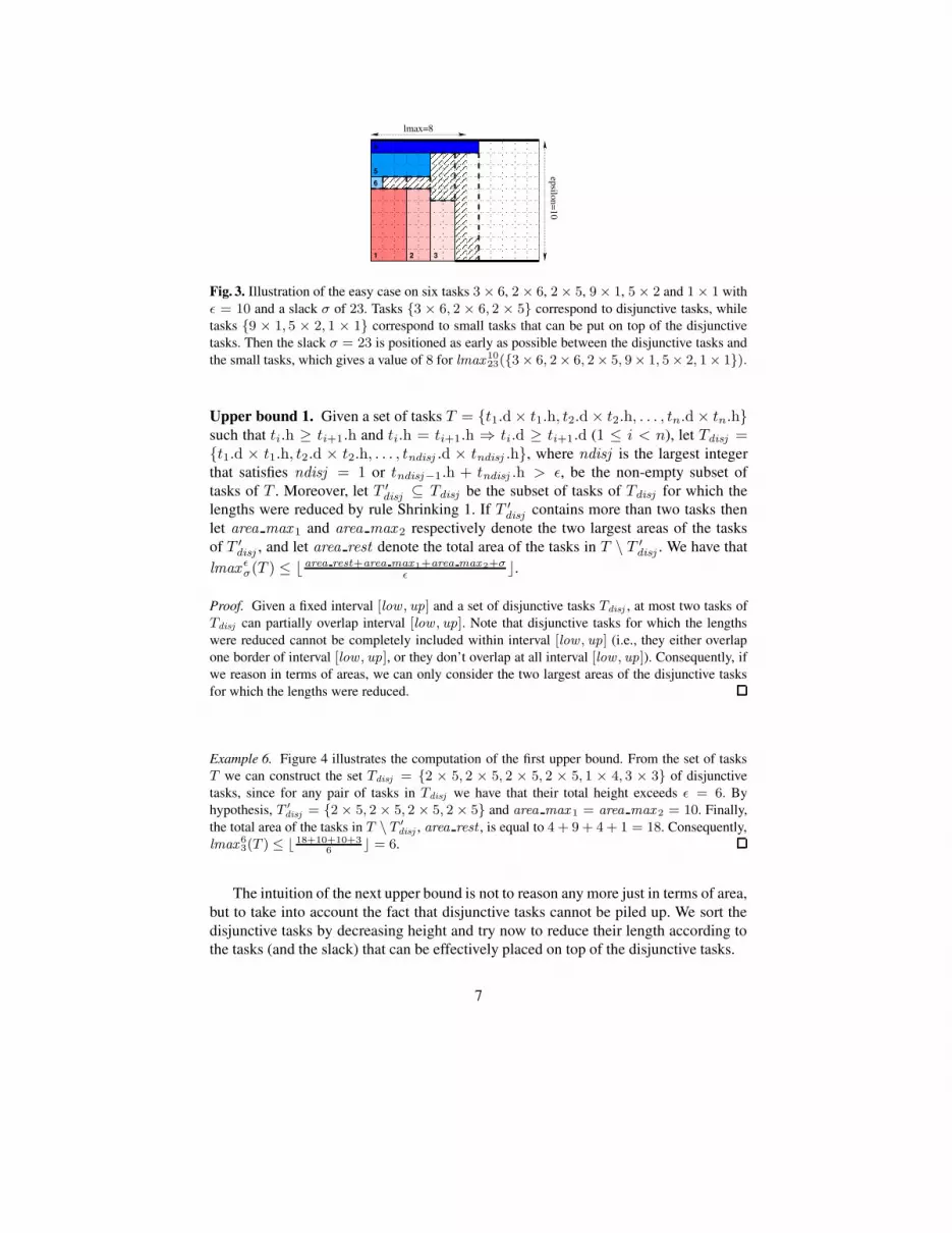
Fig. 3. Illustration of the easy case on six tasks 3 × 6, 2 × 6, 2 × 5, 9 × 1, 5 × 2 and 1 × 1 withε = 10 and a slack σ of 23. Tasks {3 × 6, 2 × 6, 2 × 5} correspond to disjunctive tasks, whiletasks {9 × 1, 5 × 2, 1 × 1} correspond to small tasks that can be put on top of the disjunctivetasks. Then the slack σ = 23 is positioned as early as possible between the disjunctive tasks andthe small tasks, which gives a value of 8 for lmax 10
23({3 × 6, 2× 6, 2× 5, 9× 1, 5× 2, 1× 1}).
Upper bound 1. Given a set of tasks T = {t1.d × t1.h, t2.d × t2.h, . . . , tn.d × tn.h}such that ti.h ≥ ti+1.h and ti.h = ti+1.h ⇒ ti.d ≥ ti+1.d (1 ≤ i < n), let Tdisj ={t1.d × t1.h, t2.d × t2.h, . . . , tndisj .d × tndisj .h}, where ndisj is the largest integerthat satisfies ndisj = 1 or tndisj−1.h + tndisj .h > ε, be the non-empty subset oftasks of T . Moreover, let T ′
disj ⊆ Tdisj be the subset of tasks of Tdisj for which thelengths were reduced by rule Shrinking 1. If T ′
disj contains more than two tasks thenlet area max1 and area max2 respectively denote the two largest areas of the tasksof T ′
disj , and let area rest denote the total area of the tasks in T \ T ′disj . We have that
lmax εσ(T ) ≤ barea rest+area max1+area max2+σ
εc.
Proof. Given a fixed interval [low , up] and a set of disjunctive tasks Tdisj , at most two tasks ofTdisj can partially overlap interval [low , up]. Note that disjunctive tasks for which the lengthswere reduced cannot be completely included within interval [low , up] (i.e., they either overlapone border of interval [low , up], or they don’t overlap at all interval [low , up]). Consequently, ifwe reason in terms of areas, we can only consider the two largest areas of the disjunctive tasksfor which the lengths were reduced.
Example 6. Figure 4 illustrates the computation of the first upper bound. From the set of tasksT we can construct the set Tdisj = {2 × 5, 2 × 5, 2 × 5, 2 × 5, 1 × 4, 3 × 3} of disjunctivetasks, since for any pair of tasks in Tdisj we have that their total height exceeds ε = 6. Byhypothesis, T ′
disj = {2 × 5, 2 × 5, 2 × 5, 2 × 5} and area max 1 = area max 2 = 10. Finally,the total area of the tasks in T \ T ′
disj , area rest , is equal to 4 + 9 + 4 + 1 = 18. Consequently,lmax 6
3(T ) ≤ b 18+10+10+36
c = 6.
The intuition of the next upper bound is not to reason any more just in terms of area,but to take into account the fact that disjunctive tasks cannot be piled up. We sort thedisjunctive tasks by decreasing height and try now to reduce their length according tothe tasks (and the slack) that can be effectively placed on top of the disjunctive tasks.
7

area_max =10
hihhihhihjjj
(C)(B)
(A)
1
2ep
silon
=6lmax<7 lmax=4
epsil
on=6
slack=3 area_rest=18
area_max =10
kikl mn op qiqrir stuiuviv7
65
8
21 1 2
8
1 2 3 4 5 6 7 8
slack=3
Fig. 4. (B) Illustration of the first upper bound on eight tasks (A) T = {2 × 5, 2 × 5, 2 × 5, 2 ×5, 1 × 4, 3 × 3, 2 × 2, 1 × 1}, where the length of the first four tasks was reduced by applyingrule Shrinking 1 (this reduction is depicted by a dashed line along the right border of a task),with ε = 6 and a slack σ of 3. (C) A placement giving the exact value for lmax 6
3(T ). Notethat a task for which the length was reduced can only be put at one of the two extremities of theplacement; consequently, we cannot add task 5 and task 7 to gain an extra unit for lmax 6
3(T )(since the lengths of tasks 1 and 2 were reduced, tasks 1 and 2 have to be kept at one of the twoextremities).
Upper bound 2. Given a set of tasks T = {t1.d × t1.h, t2.d × t2.h, . . . , tn.d × tn.h}such that ti.h ≥ ti+1.h and ti.h = ti+1.h ⇒ ti.d ≥ ti+1.d (1 ≤ i < n), let Tdisj ={t1.d× t1.h, t2.d× t2.h, . . . , tndisj .d× tndisj .h}, where ndisj is the largest integer thatsatisfies ndisj = 1 or tndisj−1.h+ tndisj .h > ε), be the non-empty subset of tasks of T .Let t1, t2, . . . , tndisj denote the tasks of Tdisj sorted by decreasing height and for any h
let areah denote the total area of the tasks of T that have a height less than or equal toh. If there is an i ∈ [1, |Tdisj |] such that:
– ∀j ∈ [1, i− 1],∑j
k=1 tk.d · tk.h + areaε−tj .h + σ ≥∑j
k=1 tk.d · ε,– ∑i
k=1 tk.d · tk.h + areaε−ti.h + σ <∑i
k=1 tk.d · ε,
then the length of task ti can be reduced to bareaε−ti.h+σ−
Pi−1
k=1tk.d·(ε−tk.h)
ε−ti.hc.
Now let T ′disj be the set of tasks derived from Tdisj by considering their reduced
length and by discarding the tasks for which the reduced length is equal to 0. Let area =∑
t∈T−T ′
disjt.d · t.h + σ and let t′1, t
′2, . . . , t
′|T ′
disj|, t
′|T ′
disj|+1 denote the tasks of T ′
disj
sorted by decreasing height, where t′|T ′
disj|+1 stands for an additional task of height 0
and length d areaε
e. In this context, let i be the smallest integer such that∑i
k=1 t′k.d ·
(ε − t′k.h) ≥ area . We have that lmax εσ(T ) ≤
∑i−1k=1 t′k.d + b
area−Pi−1
k=1t′k .d·t′k.h
ε−t′i.h c.
Example 7. Figure 5 provides an example of application of the second upper bound on a set oftasks T = {3 × 5, 2 × 4, 2 × 4, 5 × 3, 3 × 3, 2 × 2, 1 × 1} under the hypothesis that we havea slack σ = 3 and a gap ε = 6. The set of disjunctive tasks Tdisj built from these rectangles is{3 × 5, 2 × 4, 2 × 4, 5 × 3}. The length of task t3 (i.e., i = 3) can be reduced since:
8

– [j = 1]: t1.d · t1.h + area6−5 + σ = 3 · 5 + 1 + 3 = 19 ≥ 3 · 6,– [j = 2]: t1.d · t1.h + t2.d · t2.h + area6−4 + σ = 3 · 5 + 2 · 4 + 5 + 3 = 31 ≥ (3 + 2) · 6,– [i = 3]: t1.d · t1.h+ t2.d · t2.h+ t3.d · t3.h+ area6−4 +σ = 3 · 5+2 · 4+2 · 4+5+3 =
39 < (3 + 2 + 2) · 6.
The length of task t3 = 3 × 4 is reduced to bareaε−t3.h+σ−t1.d·(ε−t1.h)−t2.d·(ε−t2.h)
ε−t3.hc =
b 5+3−3·(6−5)−2·(6−4)6−4
c = 0. Consequently, lmax 63(T ) = 8 (instead of 9 if t3 is not removed).
wxwyzxzzxz{{
|x|}
(B)
slack=3
(D)
slack=3
epsil
on=6
lmax<10
epsil
on=6
epsil
on=6
lmax<5+3+1 lmax=8(C)
(A)
~� �� ��
������
�x���x����
21
56
421
4321
4321
76543
7
7 6
6
5
5
slack=3
Fig. 5. (A) Seven tasks 3×5, 2×4, 2×4, 5×3, 3×3, 2×2 and 1×1 to place with a slack of 3and a gap ε of 6, (B) An upper bound of 9 obtained without shrinking, (C) A tighter upper boundof 8 obtained by removing the third task, (D) An optimal placement which reaches the bound 8.
This second upper bound can be enhanced by trying to compute a bigger list of tasksin disjunction. A task ti cannot overlap a task tj if the sum of their heights, ti.h + tj .h,is greater than ε. But we can also use the fact that we have already computed the longestcumulative hole for smaller values of ε. Tasks ti and tj are also in disjunction if there isa gap g on top of the two tasks (i.e., g = ε− ti.h− tj .h) for which lmax g
σ(T \ {ti, tj})is equal to 0.
3.4 Illustrating the Incomparability of the Two BoundsThis section shows that the two bounds previously described are in fact incomparable.For this purpose, consider the tasks of size 2 × 2, 4 × 4, 6 × 6, 7 × 7, 8 × 8, 9 × 9,11×11 and 15×15. Let B1ε
σ and B2εσ respectively denote the upper bounds for lmax ε
σ
obtained by the first and the second upper bounds previously introduced. On the onehand, we have that B112
0 = 5 and B2120 = 4, while on the other hand we have that
B1150 = 30 and B215
0 = 32.
9

4 Balancing Knapsack ConstraintsIn the context of a cumulative(T, L) constraint with |T | = n and slack σ, let itstimespan be defined as [umin, umax] where umin = min{t.s | t ∈ T} and umax =max{t.s + t.d − 1 | t ∈ T}. If σ = 0, then for every time point b ∈ [umin, umax], thetotal height of tasks intersecting b must equal L. This reasoning can be generalized tonon-zero slack and strengthened by considering adjacent pairs of time points (b − 1, b)into the following proposition.Proposition 1. For a cumulative(T, L) constraint with slack σ and timespan [umin, umax],for every time point b ∈ [umin+1, umax], each of the following conditions is a necessarycondition for the constraint.
– Let Hb−1 denote the total height of tasks intersecting b − 1. Hb−1 ∈ [L − σ, L]must hold.
– Let Hb denote the total height of tasks intersecting b. Hb ∈ [L − σ, L] must hold.– Hb−1 + Hb ∈ [2 · L − σ, 2 · L] must hold.
Let ti denote the ith task of T . For every time point b ∈ [umin + 1, umax] and taskti ∈ T , we have four mutually exclusive possibilities. We encode these possibilities as0-1 variables Sib, Cib, Oib, Nib where Sib + Cib + Oib + Nib = 1 and:
Sib = 1 ⇔ ti intersects b but not b − 1, that is, ti.s = b
Cib = 1 ⇔ ti intersects b − 1 but not b, that is, ti.s = b − ti.dOib = 1 ⇔ ti intersects both b − 1 and b, that is, ti.s ∈ [b − ti.d + 1, b− 1]Nib = 1 ⇔ ti intersects neither b − 1 nor b, that is, ti.s 6∈ [b − ti.d, b]
(1)
For a given time point b, the set of tasks T and the above, we can set up the followingpseudo-boolean equation system, which essentially captures the above proposition.
∀i ∈ [1, n] : Sib + Cib + Oib + Nib = 1Hb−1 =
∑
i∈[1,n] ti.h · (Cib + Oib) ∈ [L − σ, L]
Hb =∑
i∈[1,n] ti.h · (Sib + Oib) ∈ [L − σ, L]
Hb−1 + Hb ∈ [2 · L− σ, 2 · L]
(2)
This equation system can be solved by a dynamic programming method similar tothe one described in [11]. Define a function f(k, l, r) equal to 1 if and only if the derivedequation system (3) has a solution, and define the dynamic programming recursion asin (4).
∀i ∈ [1, k] : Sib + Cib + Oib + Nib = 1∑
i∈[1,k] ti.h · (Cib + Oib) = l∑
i∈[1,k] ti.h · (Sib + Oib) = r
(3)
f(0, l, r) =
{
1 , if l = 0 ∧ r = 00 , otherwise
f(k, l, r) = max
f(k − 1, l, r − tk.h)f(k − 1, l − tk.h, r)f(k − 1, l − tk.h, r − tk.h)f(k − 1, l, r)
, if k > 0(4)
10

Now, intuitively, (2) has a solution if and only if there exist l and r such that l ∈[L−σ, L], r ∈ [L−σ, L], l+r ∈ [2 ·L−σ, 2 ·L], and f(n, l, r) = 1. One can visualizethis as a directed graph with a node for every (k, l, r) for which f(k, l, r) = 1 and arcscorresponding to (4). Also, each arc is annotated with the 0-1 variable that is assumedto take the value 1 in that branch of the recursion:
(k − 1, l, r − tk.h)Skb
// (k, l, r)
(k − 1, l − tk.h, r)Ckb
// (k, l, r)
(k − 1, l − tk.h, r − tk.h)Okb
// (k, l, r)
(k − 1, l, r)Nkb
// (k, l, r)
Among the nodes, let the single source node be (0, 0, 0), and let the sink nodes beall nodes (n, l, r) where l ∈ [L−σ, L], r ∈ [L−σ, L], and l+r ∈ [2 ·L−σ, 2 ·L]. Thena path from the source to some sink corresponds to a solution to (2). By inspecting thearcs of such paths, we can determine for each 0-1 variable whether it takes the value1 in some solution to (2). After computing all paths, we inspect each 0-1 variable: if itdoes not take the value 1 in any solution, the corresponding start time domain is prunedaccording to the equivalences given in (1). The complexity of this algorithm is O(nL2)(space and time).Example 8. Consider a cumulative({t1, t2, t3}, 6) constraint with tasks as defined in Figure 6.Let us apply the method for b = 4 and σ = 4 (the slack has been tightened by other, fixed tasksthat have been omitted in the example). The method explores the digraph shown in Figure 6. Thefour sink nodes are denoted by ellipses. As there is no arc annotated with O3b on a path reachinga sink, we conclude that t3 cannot intersect both 3 and 4, hence the value 3 can be removed fromD(t3.s). In this example, the digraph is a tree, which is not generally the case.
4.1 Strengthening the MethodThe method can be strengthened by adding more knapsack constraints, e.g., constraintsthat capture the fact that the height of the cumulative profile must not exceed L. Thiscan be done as follows:
– Identify subsets Tl ⊆ T and Tr ⊆ T such that the following properties hold:• For each ti ∈ Tl, both 0 and 1 are feasible values for Oib, and Oib = 0 would
create a compulsory part of ti to the left of b.• If Oib = 0 for all ti ∈ Tl, the cumulative profile would exceed L.• For each ti ∈ Tr, both 0 and 1 are feasible values for Oib, and Oib = 0 would
create a compulsory part of ti to the right of b.• If Oib = 0 for all ti ∈ Tr, the cumulative profile would exceed L.
– Add the knapsack constraint∑
ti∈TlOib ≥ 1 for every such subset Tl found.
– Add the knapsack constraint∑
ti∈TrOib ≥ 1 for every such subset Tr found.
Our implementation includes this idea, using at most one subset Tl and at most onesubset Tr.
11

D(t1.s) = {3}, t1.h = 4, t1.d = 3D(t2.s) = {2, 3, 4}, t2.h = 2, t2.d = 2D(t3.s) = {1, 3, 4}, t3.h = 1, t3.d = 2
(0,0,0) (1,4,4)O1b
(2,4,6)S2b
(2,6,6)O2b
(2,6,4)
C2b
(3,4,7)S3b
(3,5,7)O3b
(3,4,6)N3b
(3,6,7)S3b
(3,7,7)O3b
(3,6,6)
N3b
(3,6,5)S3b
(3,7,5)O3b
(3,6,4)
N3b
Fig. 6. Tasks and digraph explored by dynamic programming for b = 4, σ = 4, L = 6.
4.2 Learning Solutions
Let the pre-signature of a cumulative(T, L) constraint and time point b be the set of 0-1variables for which the value 1 is feasible according to (1) prior to solving the equationsystem. Similarly, let its post-signature be the set of 0-1 variables for which the value 1is still feasible after solving the equation system.
It is worth noting that, given fixed T, L, σ, the pseudo-boolean equation systemis totally abstracted away from the chosen b as well as from the variable domains. Itis totally determined by its pre-signature. Thus having solved an equation system, itmakes sense to record its pre- and post-signatures. Later on, if an equation system withthe same pre-signature arises, we can retrieve the associated post-signature instead ofrecomputing it. Experience shows that this idea saves about 75% of the computationaleffort.
5 Performance Evaluation
All the new filtering methods described in this paper were integrated into our geost ker-nel [12] in order to strengthen the sweep-based filtering associated with non-overlappingconstraints. The experiments were run in SICStus Prolog 4 compiled with gcc -02 ver-sion 4.0.2 on a 3GHz Pentium IV with 1MB of cache. All benchmarks were run with thefollowing four phases search procedure, where at each phase, rectangles are consideredby decreasing area. Let o.x denote the X coordinate variable of the rectangle o:
1. For each rectangle o, narrow by binary search the domain of o.x until it has acompulsory part that is at least half the length of o.
2. For each rectangle o, fix o.x by binary search.3. Repeat steps 1-2 for the Y coordinates.
12

Wanting to get an idea of their performance on perfect packing problems (i.e., 0%slack), we considered the perfect square problem [1, 9]. A perfect square of order n isa square that can be tiled with n smaller squares where each of the smaller squares hasa different integer size. We used the data available (i.e., the size of the small squares topack) from the catalogue [13] and tested the corresponding 207 instances. On the onehand, 66 problems were completely solved (i.e., finding all solutions and proving thatno other solution exists) without a single backtrack. On the other hand, 36, 84, 20, resp.1 problems were solved by using 1-10, 11-100, 101-1000, resp. 1001-1438 backtracks.This is an improvement by two orders of magnitude over [12]. From a time point ofview, 35, 169 resp. 3 problems were solved in less than 10, 100 resp. 200 seconds.
In order to evaluate our method on non-perfect packing problems (with non-zeroslack), we took 202 out of the same 207 perfect square instances, removing in each in-stance the smallest square to place. Five instances were excluded because they exceededthe time limit.
To evaluate the effectiveness of the two methods described in this paper, Figure 7summarizes per benchmark set the performance. Square 1 denotes searching for thefirst solution of a perfect square with symmetry breaking, whereas Square N denotessearching for all (8 or 16) solutions of a perfect square instance with no symmetrybreaking, and Butone N denotes searching for all solutions of a perfect square instancewith the smallest square removed, also with no symmetry breaking. The figure alsocontains six scatter plots. Each dot corresponds to a problem instance. Its X coordinateequals the number of backtracks to solve it with both methods enabled. Its Y coordinateequals the number of backtracks to solve it with only one method enabled.
On the perfect square instances, we find that both methods sharply decrease thenumber of backtracks, balancing knapsack constraints having the strongest effect. Onthe non-perfect packing instances, the results suggest that the effectiveness of balancingknapsack constraints degrades somewhat more rapidly with increasing slack than thatof the longest cumulative hole method. In both cases, we find a nice multiplicativeeffect from combining the two methods. However, when we tried the methods on the2D orthogonal packing instances proposed by Clautiaux et al. [7], the two methods didnot significantly decrease the number of backtracks on non-perfect packing instances,whereas on instances with zero slack they did. So the results should be treated withcaution for non-perfect packing problems.9
6 Conclusion
This paper introduces two new filtering methods that can be used in the context of thecumulative as well as the non-overlapping constraints.
1. The longest cumulative hole problem can be used to detect early that some specificspace can not be filled enough.
2. The balancing knapsack constraint relates the total height of the tasks that end at agiven time point to the total height of the tasks that start at the same time point.
9 Unlike the squares instances, it is worth noting that Clautiaux instances contain rectangles thatare long in one dimension and short in the other dimension.
13

Set Ghk Gh Gk G
Butone N 170730 (29637) 275445 (25013) 520050 (94205) 1383888 (107317)Squares N 10043 (4168) 96213 (10951) 17417 (5470) 1006336 (86080)Squares 1 996 (1557) 9730 (1203) 1817 (1840) 151905 (11813)
1
10
100
1000
10000
100000
1 10 100 1000 10000 100000Butone N: Ghk vs. Gh
1
10
100
1000
10000
100000
1 10 100 1000 10000 100000Butone N: Ghk vs. Gk
1
10
100
1000
10000
100000
1 10 100 1000 10000Squares N: Ghk vs. Gh
1
10
100
1000
10000
1 10 100 1000 10000Squares N: Ghk vs. Gk
1
10
100
1000
10000
1 10 100 1000Squares 1: Ghk vs. Gh
1
10
100
1000
1 10 100 1000Squares 1: Ghk vs. Gk
Fig. 7. Top: performance summary as total backtracks (seconds) per benchmark set. Bottom:scatter plots of number of backtracks per instance. X coordinate values correspond to probleminstances with both methods enabled. In the left hand column, balancing knapsack constraintswere knocked out in the Y coordinate values. In the right hand column, the longest cumulativehole method was knocked out in the Y coordinate values. Ghk, Gh, Gk and G denote respectivelythe geost kernel with both methods, with longest cumulative holes only, with balancing knapsackconstraints only, and with neither method added.
14

As demonstrated by our benchmarks, these two methods are complementary, es-pecially when the slack is very small. In such contexts, they reduce significantly thenumber of backtracks and even allow to completely enumerate the search space for asignificant number of instances without any backtrack. An open issue is to come upwith more efficient methods for proving infeasibility when the slack is not so small.
Acknowledgements
This research was conducted under European Union Sixth Framework Programme Con-tract FP6-034691 “Net-WMS”.
References
1. A. Aggoun and N. Beldiceanu. Extending CHIP in order to solve complex scheduling andplacement problems. Mathl. Comput. Modelling, 17(7):57–73, 1993.
2. Y. Caseau and F. Laburthe. Cumulative scheduling with task intervals. In Joint InternationalConference and Symposium on Logic Programming (JICSLP’96). MIT Press, 1996.
3. L. Mercier and P. Van Hentenryck. Edge-finding for cumulative scheduling. INFORMSJournal on Computing, 20(1), 2008.
4. A. Lahrichi. Scheduling: the notions of hump, compulsory parts and their use in cumulativeproblems. C.R. Acad. Sci., Paris, 294:209–211, February 1982.
5. F. Clautiaux, A. Jouglet, J. Carlier, and A. Moukrim. A new constraint programming ap-proach for the orthogonal packing problem. Computers and Operation Research, 35(3):944–959, 2008.
6. M. Biro. Object-oriented interaction in resource constrained scheduling. Information Pro-cessing Letters, 36(2):65–67, 1990.
7. F. Clautiaux, J. Carlier, and A. Moukrim. A new exact method for the two-dimensional or-thogonal packing problem. European Journal of Operational Research, 183(3):1196–1211,2007.
8. N. Lesh, J. Marks, A. McMahon, and M. Mitzenmacher. Exhaustive approaches to 2d rect-angular perfect packings. Information Processing Letters, 90(1):7–14, 2004.
9. P. Van Hentenryck. Scheduling and packing in the constraint language cc(FD). In M. Zwebenand M. Fox, editors, Intelligent Scheduling. Morgan Kaufmann Publishers, 1994.
10. N. Beldiceanu and E. Contejean. Introducing global constraints in CHIP. Mathl. Comput.Modelling, 20(12):97–123, 1994.
11. M. A. Trick. A dynamic programming approach for consistency and propagation for knap-sack constraints. Annals of Operations Research, 118(1–4):73–84, 2003.
12. N. Beldiceanu, M. Carlsson, E. Poder, R. Sadek, and C. Truchet. A generic geometricalconstraint kernel in space and time for handling polymorphic k-dimensional objects. InC. Bessiere, editor, Proc. CP’2007, volume 4741 of LNCS, pages 180–194. Springer-Verlag,2007.
13. C. J. Bouwkamp and A. J. W. Duijvestijn. Catalogue of simple perfect squared squares oforders 21 through 25. Technical Report EUT Report 92-WSK-03, Eindhoven University ofTechnology, The Netherlands, November 1992.
15


