The Martian magnetotail

4d~.Space Res. Vol ~. No. 1. pp 301—314. 1986 073—11~786 S0.l~) .50Pnnted in Gmat Brttain. All rtnhts resersed. Copsnght © COSPAR

THE MARTIAN MAGNETOTAIL

0. VaisbergandV. Smirnov

SpaceResearchinstitute, U.S.S.R.AcademyofSciences,117810Moscow, U.S.S.R.

ABSTRACT

There is evidence of a strong influence of an atmospheric (cometary) interaction on theMartian tail formation: small total magnetic flux in the tail, the existence of plasma flowof apparently planetary origin, interplanetary magnetic field control of magnetic fieldorientation in the tail and other evidence. At the same time the large radius of theMartian magnetotail (about 2 planetary radii) can be considered as a strong evidence forthe existence of a planetary magnetic field. Plasma and magnetic field properties in theMartian tail are in many respects similar to the ones observed in the tail of Venus. Thelimited amount of near-Mars measurements leads to some reservations in coming to definiteconclusions. A combined magnetosphere of Mars is suggested that consists of two polar-tiedmagnetic tubes connected to the tail and an equatorial Venus-type interaction region in-between.

INTRODUCTION

From the study of different magnetospheric systems we know two clear-cut cases: one thatarises from solar wind interaction with (nearly orthogonal to the flow) a magnetic momentof the planet, i.e., terrestrial magnetosphere (see for example /1,2/), and another oneresulting from solar wind interaction with a planetary atmosphere, that, for the case ofVenus, is the limiting case of a cometary type interaction /3,4/. Any obstacle to solarwind flow creating a substantial disturbance in this flow develops the tail or wake withcharacteristics determined both by the nature of obstacle and by parameters of the externalflow. A crucial role in the determination of the topology of the tail is played by themagnetic field. For a strong enough planetary field two lobes of the tail are tied tothe polar regions of the planet while the tail of a field—free planet rotates around thesolar wind flow direction with changes in the IMF direction /3/.

From the point of view of solar—planetary studies, Mars is an unlucky planet. In spite ofthe significant number of spacecraft launched to Mars in the first two decades of thespace era, we do not know very much about the Mars environment. Previous Soviet andAmerican space programs did not provide enough room for measurements of particles and fields.We spent much effort during the preparation of Mars 2-3 /1971-1972/ and Mars 4-7 /1973/programs advocating before the planetary community the importance of studies of the Marsenvironment. There were similar but unsuccessful attempts by American scientists toinclude a magnetometer in the Viking program /1976/.

Nevertheless, one fly—by mission, three orbiters and two landers had instrumentation forthe measurement of particles and fields in the Mars environment. Besides that severalspacecraft were used to investigate the ionosphere of Mars by radio—occultation technique.Yet the data we have are relatively scarce. The orbits of Mars—bound satellites werechosen without allowance for magnetospheric studies. The instrumentation of the seventies wasnot sophisticated enough and the telemetry rate was insufficient. These are the reasonswhy when discussing the Martian tail we are often forced to use indirect arguments. Pri-marily, we do not know much about the magnitude and orientation of Martian magnetic moment.

The plan of this paper is the following. After a brief description of the experiments per-formed we will discuss what we know about the Martian magnetic field. Then in succession,magnetic and plasma measurements in the Martian tail will be considered. Finally, we willdiscuss the present state of knowledge and some speculations about solar wind—Marsinteractions.

301

302 0. Vaisbergand V. Smirnov

tiE

I 1432~10 100

I ___________ _____

MT 1410 1420 1430 1440 1450 1500 100 1000

Rii~~km) 7 ~ I E~/Q 1eV)60 40 2525 40 60

10

/~ 1557

01/08/72 1357 /> ~— MP

Mars 2 )/?~57; ~ hJR0 - 0.2

~ 14~~ 0

X (i0~km)

Fig. 1. Profiles of magnetic field strength (a), electron fluxes (b) and ion fluxes (c)along the orbit of Mars—2 on January 8, 1972. The orbit of the satellite is shown belowin a cylindrical coordinate system with the x—axis directed towards the Sun. HO—analogyshock and magnetopause are adjusted to shock crossing (A) and to ion cushion traversals(B and C). Two panels on the right-hand side show selected electron and ion spectra aboveand inside the obstacle.

A SHORT HISTORY

During the first fly-by mission, of Mariner-4 in 1965, magnetic measurements /5/ revealedtwo crossings of bow shock. Subsequent interpretation of these data in terms of the gasdynamic analogy /6,7/ gave the first estimates of internal magnetic field of Mars.

In 1971-72 two orbiters: Mars-2 and Nlars—3 performed measurements of magnetic field andplasma in the neighbourhood of the planet /8—10/. The spacecraft approached the planet nocloser than ellOO km on the dayside. The permanent existence of the bow shock was firmlyestablished /10,11,12,13/, implying a hard type of solar wind — Mars interaction withessentially a nonabsorbing obstacle /14/. Several passes of the Mars-2 and —3 spacecraftthrough the region of enhanced, up to ‘i~3Oy, magnetic field on the dayside of the planetincluding one pass of Mars-3 in its three—axis stabilized orientation allowed Dolginov andco—workers /8/ to state the existence of Martian magnetic field. A layer of moderate-heated ions on the dayside (plasma cushion) was found /9/ and a similar plasma regime inthe remote night-side region revealed the existence of the Martian tail /15/.

The last Martian orbiter carrying magnetic and plasma experiments - Mars—S - operated inearly 1974. Magnetic measurements allowed Dolginov and co—workers to strengthen theirarguments in favour of the internal origin of Martian field /16/. The plasma populationin the Martian tail was studied in some detail /17—21/ as well as the bow shock and externalflow /14,19,21,22/.

The properties of the ionospheric plasma on the dayside of Mars were measured directly ontwo Viking probes in 1976 /23/. Less direct but more numerous radio-occultation ionosphericprofiles were obtained on Mars and Mariner spacecraft /24-28/. Although these data arenot directly relevant to the topic of the Martian tail they contributed significantly tothe understanding of the Martian environment.

Martian Magnetotail 303

1 5 10 15(a) I I I ,.~_ (b)

B lo c /A

2O~ ~ 2- ~14~

10 _A.f.:~~/_\I~Bxi 1 — 2 16•.15

I S S

_________________ ~ I I 19 18 170 ~ ~ 0 Cos2 0.4 016

-10 — (d) L __________ (e) A

(c) •J’~Z

5~ (lO

3km) ZSE(!O km)101 - 10Um~ e 10 ~ 1 15 t~

3

H io~ 2~1 ~ ~.5 -~ X;E~~51~

Moscow Time

Fig. 2. Summary of January 21, 1972 Mars—3 pass through Martian magnetosphere. Magnitudeand BxcOmponent of magnetic field, b—magnetic field pressure versus quasi—Newtonianpressure approximation, c—curves of soft electron current

1e~ soft ion counting rate Jj,and the difference between straight line approximation of B~/8sr (line “A’) through thepoints 1—7 and the calculated one from measured values at points 8—19, d-orbit of Mars—3in a cylindrical coordinate system and adjusted magnetopause crossings, e—projectionof observed magnetic field vectors on solar-ecliptic XY-plane. Lines B and C “magneto-pause” crossings, line U — separation line between the ‘planetary” and induced parts ofthe magnetosphere.

MAGNETIC FIELD OF MARSAND DAYSIDE PLASMA

The decisive role of the origin of the magnetospheric field in the determination of tailproperties is well known. First we shall discuss the evidence for the internal origin ofthe Martian field. The very close location of the bow shock to Mars shows that, if Marshas a magnetic moment, its magnitude is marginal in terms of sustaining the solar wind rampressure /14,15,29/. The first suggestion of the existence of something additional to theionospheric pressure to standoff the solar wind from the planet using the first determi-nations of bow shock location was made in /9/ as the shock appeared to be standing somewhatfarther from Mars than the ND model with ionospheric obstacle predicted. Since then manyspears have been broken on whether the bow shock location may be used as a firm indicationof the obstacles dimension /21,30,31/. In spite of some success of the HO—analogy in theexplanation of the relative location of the Venusian bow shock and ionopause /32/ manyquestions of the applicability of this approach to such small and complicated systemsseems to remain. They include the existence of the magnetic barrier and-mantle above thei000pause, the pick up of atmospheric ions and, last but not least, the small distancebetween the shock and the obstacle. The large scale of the complete ion thermalizationprocess behind the shock /33/ combined with several possible ways of energy losses in post-shock flow can modify Rankine—Hugoniot conditions and question the applicability of thecommonly used flow models.

Different HD-Analogy estimates of the effective height of the subsolar point of the Martianobstacle to the solar wind ranged from x35O km /6,12/ to sI200 km /13,30/ with more recentfigures about 600 km /14,29,34/. Even the possibility of estimating the mean height ofthe obstacle was questioned /31/. The termination of the solar wind flow and its replace-ment by the lower energy plasma regime was observed on 5 of 8 dayside passes of Mars-2 andMars-3 /14,35/. This termination usually occurred at heights of 1350+150 km for solar-zenith angles (SZA) 200_600 (3 passes), but was significantly higher on two passes(1700-2300 km at SZA 450_650). Three passes of Mars-2 did not reveal any sign of theobstacle to the external flow at a height >1100 km and SZA range 200_600. Figure 1 illus-trates the observations made on early Marsspacecraft /14/. The crossing of the bow shockon the inbound leg of the Mars-2 orbit occurred at 1407 MT (Moscow Time) on January 8th,1972. Coming closer to the subsolar point Mars—2 entered a region with increased magneticfield. This was accompanied by a decrease of the solar wind ion flux and by the appearanceof low energy ions (ion “cushion” /12/) and electrons as well as by a softening of theelectron energy spectrum. Closer to the planet the satellite entered a region where theenergy of ions dropped below 27 eV (lowest energy step of RIEP plasma spectrometer). Thenthe events repeated in the reverse order. Matching different regions to HO—analogy /37/suggests that the ion “cushion” is situated slightly above (~3OO km) the effective HO—obstacle to the external flow /35/.

304 0. Vaisberg and V. Smirnov

4 12/17/71 M2

1 12/15/71 M2 5 1Z’18/71 M2

2 01/08/72 M2 1 ~ 6 02/24/72 M2

3 0121/72 M3 15 ~ 15 —

Bow shock crossing -‘t’~/”

tl

— No ions Ct1 30 eV)

— Obstacle CE1 < 30eV) //// ~o-

X (iO~km)

Fig. 3. Extreme locations of the Martian magnetopause and shock: a — inflated magneto-sphere with HO—boundaries adjusted to observed ones and b - compressed magnetosphere.

Another example of a dayside crossing of the Mars magnetosphere is shown on Figure 2. Thisis a modification of the analysis performed in /38/. The plasma behaviour in the “magneto-sphere”, i.e., between the two “magnetopause” crossings identified by Dolginov /36/ isasymmetric. Because satellite Mars—3 passed close to the obstacle boundary, the magneticfield may be compared with the Cos

2’V law (‘P—SZA angle). It is clear from Figure 2, thatonly part of the magnetic field profile within the magnetosphere (until 21—43 MT) followsthe Cos~Cbehaviour. The deviation of B2/8w from the Cos2C law is accompanied by theappearance of hot “cushion” ions /12/ and increased fluxes of electrons /37/. This is avery clear example of what can be considered as the “combined” magnetosphere /21/ with partof it controlled by internal—sources field and part of it formed by the induced magneticfield. It is exactly this pass of Mars-3 that allowed Dolginov et al. /8/ to state thatMars has a magnetic field with a magnetic moment 2.55x1O22 Gs.cm3 and with coordinates ofits magnetic north pole 4 = -17° and A 3000.

This estimation was done without any allowance for magnetopause currents and the inferredmoment may be in error with a factor of “~ 2 /39/. Indeed, calculations made in /38/showed that the modelling of the external sources by a homogeneous magnetic field givesM

0 a 1.6 x 1022 Gs.cm3 and 4 = 20°, x = 800 not changing the orientation of the dipole

markedly. It could be seen also from Figure 2 that both parts of the “magnetosphere” showclear draping. This draping allowed Russell /40/ to question the statement that Mars-3entered the magnetosphere of Mars. Figure 3 summarizes the limiting cases of the geometryof the dayside observations. Passes of Mars-2 and Mars-3 through the region from whichthe solar wind flow was excluded were usually accompanied by more distant crossings of theshock. Plasma, nearly stationary and colder than surrounding flow, was observed at orabove the effective HO—obstacle. When Mars—2 passed definitely above the obstacle theshock tended to be closer to the planet. It is worth noting that the shock and obstacleboundary locations at Mars are barely sensitive to solar wind ram pressure /41/.

It was shown /12/ that the pressure of plasma inside the “cushion” is large enough to con-tribute to the pressure balance, constituting about 0.3 of the total value necessary tocompensate the solar wind ram pressure. It is confirmed by the following procedure wherean additional pressure term was calculated from the deficiency of the magnetic pressurecompared to the Cos28’ law applied to the left—hand part of “magnetosphere” (Figure 2).It is seen that the calculated pressure addition closely resembles the profiles of hot“cushion” ions and electrons. It is interesting to note that 8 “~ 0.3 is also characteristicof the Venusian dayside mantle /42/. So the induced part of dayside Mars magnetospherehas a lot in common with the Venusian magnetic barrier.

It is quite clear that the ionospheric pressure alone can not sustain the solar wind rampressure /29/. Figure 4 demonstrates that for Te/Ti2.5, like that in the Venusian iono-sphere /43/, the pressure at the ionospheric maximum at SZA a 45° reaches (5—8)xlO-9dynes/cm2.This value, allowing for the external pressure drop with SZA, is below the average solarwind pressure, lxlO8dynes/cm2 (about 1/2 of the value at 1 AU /44/).


vi. — vi

iol io2 io~ ~o’10_jo

e ,cm~ Me~li,d~ne~/cm2

kT1,’K

Fig. 4. a - observed ionospheric height profiles with Viking I (Vi) and Viking 2

(2) landers. b — calculated ion thermal pressure

Thus solid majority of evidence from the observations made at the dayside of Mars suggeststhe existence of a magnetic field of internal origin with an uncertain magnitude andorientation of the magnetic moment. At the same time there is clear evidence of atmosphericinteraction resembling the now well—studied case of Venus.

MAGNETIC FIELD IN THE TAIL

Like the Mars-2 and Mars-3 orbits grazed the dayside of the Mars magnetosphere, the Mars-Sorbit during the short period of observations in early 1974 passed just below the boundaryof the Martian tail. The first evidence of Martian tail was obtained at the apocenter ofthe Mars-2 orbit when it came closest to the Sun-Mars—line on the nightside of the planet.It was identified by the appearance of low energy (tens of eV) ions /15/ not observed in theMartian magnetosheath and earlier found on the dayside of Mars /9/. Figure 5 combines thesedata with the subsequent analysis of simultaneous magnetic measurements /45/ that alsoclearly demonstrate two regions of relatively stable and enhanced Bx-component. Theregion of low—energy ions is adjacent to the region of stable enhanced positive Bx—componentas observed on February 23, 1972. No similar ion fluxes were observed on February 24thduring the following revolution of Mars—2. The tail crossing occurred 18 hours later butthe sign of Bxcomponent changed. This change of sign and the sense of Bx—component arecompatible /45/ with the earlier determination of the near-equatorial orientation of Marsdipole /8/. Later Dolginov et al. /46/ questioned the statement that Mars—2 crossed themagnetic tail of Mars during these two passes.Figure 6 shows typical examples of the magnetic field measurement in the tail, when Mars—Scrossed it at the distance I to 3 RM behind the planet. The relative stability of theBx—component allowed Dolqinov et al. /47/ to strengthen their arguments in favour of theinternal origin of the Martian magnetic field. They used the fact that Bx does not changesign with the change of the Bx-component of the IMF (although it was more natural to comparethese data with the Byz-component of the IMF). Yet to incorporate Mars-5 observations ofthe magnetic field in the Mars tail into the internal field concept Dolginov et al. /47/were forced to change the orientation of Mars-dipole and their estimate of the North polelocation was ~ a 75° and A a 2700 /30, 46/.

One important property of the magnetic field observations in the tail was that the regionwith opposite Bx polarity was observed on several orbits of Mars-S when it passed closer tothe terminator region. It was suggested in /45/, that the reversal of the sign ofBx-cclmponent observed in these cases may be associated with crossings of a cusp—like region.That means that the orientation of the Mars dipole is closer to the first estimates ofDolginov et al. /8/. The observed changes of the Bx—component sign occurred at near-equatorial latitudes of Mars. It was noticed in /46/ that similar changes were observedwith Mars—2 on the dayside of Mars. This seems to be incompatible with a nearly equatorialdip’ Ce orientation and will be discussed later. The magnitude of the magnetic field in thetail varied between 5 nT and 15 nT with an average value of about 10 nT. The magneticfield in the Mars tail was in most cases higher than in the surrounding flow. In thissense the Mars tail differs markedly from the induced tail of Venus.

0. Vaisberg and V. Smirno~

—--170eV~F~109 ID 11 12 \.~~)) ‘~~V

MT -~~\ ~I”~ ~ ~_~:~—~II /111

10 .

10 I ftD ~‘ F’

I I I , I , I\, I(nT) 07 11 15 19 03 I 07

~10’

02/23/72 02/24/72

5OO0~O7E~b23 I ~ 23 1

03 Feb. 24 tO

I , I I I5000 V X 5000 -15000

Fig. S. Bxcomponent profile along two orbits of Mars-2 on February 23/24, 1972 (in themiddle), soft ions counting rate profile and sketches of Mars dipole and tail (above).Mars-2 orbit is shown below.

At the same time there is one important property of the Martian tail that draws togetherMars and Venus. This is the existence of a significant component of the magnetic fieldtransverse to the tail axis /41/ that is essentially negligible in the “pure” magnetosphereof the Earth /48/. This is shown in Figure 7 in the rotating coordinate system determinedby the IMF-component Byz perpendicular to the solar wind flow. It was found that thedirection of the component of B transverse to the tail axis is strongly influenced by theIMF direction /41/. Clear evidence of field line draping in the Martian tail was found/49/. Figure 7 suggests that it is a rotational component implying the existence of adowntail electric current with density about 3.10—13 Amp/cm

2 /21,41/. A more accurateestimate gives the value (1 to 2)x1013 Amp/cm2. This current was suggested for thecompensation of charge-separation or ion losses of the solar wind impinging on theatmospheric obstacle /21/.

~ 4&~j.~ 15i~274 ~O.C234 ~&O234

~E~Ht____~

2I~ a~os2tc~ 22o~ ~ eiia OzLq O3.4~ 054 O&1~o5t.f~

Fig. 6. Magnetic field components and magnitude along selected orbits of Mars-5. Regionsof tail crossings are bracketed (1-in, 2-out).


i~

A r~5t ___ __

~

Fig. 7. Component of the magnetic field transverse to the tail axis in the tail of Marsand in the tail of Venus is shown in a rotated coordinate system with the direction of theIMF component transverse to the solar wind flow as one of principal axes. (View from thetail).

An important parameter is the cross-section of the Mars tail /41/. While the diameter ofthe Venusian tail is only “ 20% larger at terminator than the radius of the planet /3/,the tail of Mars is at the same cross—section about 1.8 of the Martian radius /41/. Thiswas considered to be significant evidence for the internal origin of the field in the tail/14/. It is shown in Figure 8 that the flaring angle of the tail is about 6°which com-pares favourably to the tail of the Earth /50/ and to the tail of Venus /3/ and shows thatthe magnitude of the flaring angle of the tail is the same for any type of obstacle to thesolar wind flow (the same seems true for the comets as it is suggested by comet Halleypictures).

The use of the magnetospheric similarity criterion /2/ allows us to estimate, the magneticmoment of Mars from the transverse dimension of the magnetosphere. It givesMM a 1.1022 0 cm3 /45/. Another estimate can be obtained from the total magnetic flux inthe tail. Using the classical approach of the calculation of the last closed field lineon the dayside from the subsolar radius of the magnetosphere, the cross-section of thetail a 11,000 km and the tail field magnitude 10 nT we obtain M~

1 a 3.1O2IG cm3. This

value may be subject to error by a factor of 2 due to the unknown latitude dimension of thepolar cusp and the imprecision in our knowledge of the transverse field component in thetail.

\/12÷Z

2, 1o~~ 6

X/F~0

/ [~ —2 —3 —4 —5 —6 —7 —8x, 10km.’ ‘ “ I

5 0 —5 —10 —15 —20 —25

Fig. 8. The boundary of Martian tail as obtained with Mars-2 data (low-energy ion regime),X/Ro > —4.5 and with Mars-S data (boundary between external and internal flows),X/R < -4.5. The flaring angle is shown above.

308 0. Vaisberg and V ~mtrnov

Y, 4O5krn

/

I A~.c~!T~.I~l_ ~

Fig. 9. a — Model of Mars magnetic field obtained with three sources (internal dipole,mirror dipole and cross—tail current) and adjusted to the observed obstacle boundaries(see text), and b - “bald-spot” or “bald-band” qualitative model suggested by observations.

Using a magnetospheric model approach with two external sources of the field: surface cur-rents represented by a mirror dipole and crosstail current similar to /51/ we may selectthe parameters of these sources and the value of magnetic moment of Mars to fit the observeddimensions of the Martian magnetosphere. The resulting model is shown in Figure 9a and hasthe following parameters: magnetic moment M = 1.S.lO~2G cm3, tail field magnitudeBr 12.5 nT, location of the forward edge of the tail current XT = 1.1 RM, relative magni-tude of magnetic moment of the mirror dipole, 90, and its location X

1 = 5.5 R~. Thismodel is relatively crude as it does not include the effects of the induced field thatwere clearly observed near Mars.

If the conclusion of the near—equatorial orientation of Mars dipole is correct, the Marsdipole sometimes will be aligned with sunward direction. In this respect, the Mars magne-tosphere would resemble that of Uranus. This possibility was considered in /45/ on thebasis of magnetic field topology.

PLASMA IN MARS TAIL

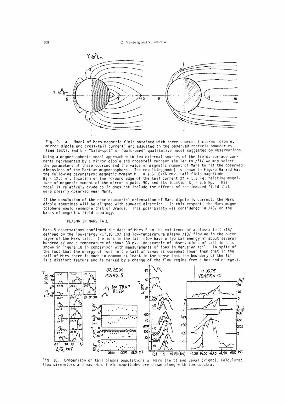
Mars-S observations confirmed the data of Mars-2 on the existence of a plasma tail /15/defined by the low-energy /17,18,19/ and low-temperature plasma /18/ flowing in the outerlayer of the Mars tail . The ions in the tail flow have a typical energy of about severalhundred eV and a temperature of about 30 eV. An example of observations of tail ions isshown in Figure 10 in comparison with measurements of ions in Venusian tail. In spite ofthe fact that the energy of ions in the tail of Venus is somewhat lower than that in thetail of Mars there is much in common at least in the sense that the boundary of the tailis a distinct feature and is marked by a change of the flow regime from a hot and energetic

— ____ Q2.2574 0 1~.O6.TS~ 307 °~“~ 04.47 ~ I MARS5 VENERA10

3 ~ ,~ ., ~ ~ .‘~\ ...

°“~ °“~ ,.r,~Ion TRAP ?A4o -~4o

~ °~~ •.•

~ _ ___

01’ ;o 04 50

E/Qk2V ______ I/ 0 ______~.00 ~ ~ lii ~ ~oEftI,keV. +4.20 ~4.3o4!f~4Q 44.50 4S~

Fig. 10. Comparison of tail plasma populations of Mars (left) and Venus (right). Calculatedflow oarameters and maqnetic field maqnitudes are shown along with ion spectra.

Martian \lagnetotail 309

Mars 5 February 20, 1974

~ 0.3~

0030 0100 0130 0200 0230 MT

I I I II1!1I~ —

10 ~ ~ . •••~•••‘••~~• -

0 t360 :‘~~~.“‘

180~ . ...• -

10 •.~‘ • -

—S. • • — •~ ••0.1 — • • .~

0300. • .

-

0100 020000 —.. . •=uS’ ~ I , I

0130 0200 0230 MTFig. 11. Energy-time spectrograms of light (L) and heavy (H) ions are shown along theMars—S orbit on February 20, 1974. Graphs show (from top to bottom); magnetic fieldmagnitude, angle between the magnetic field vector and solar direction, estimate of theratio of heavy ions number flux to light ions number flux, energy of convective motion.Mars—5 orbit is shown in the bottom left.

external flow to a lower temperature and less energetic ion flow in the tail. This ismarkedly different from what we know about the magnetospheric tail plasma flow adjacent tothe magnetopause: a plasma mantle that is mainly distinguished from the external flow bya decrease of the number density but maintaining a high ion temperature /52/. In the caseof Mars the ion number density (calculated from measured energy spectra with the sup-position that observed ions are protons) also drops contrary to the number density deter-mined from the electron spectra /19,53/. This led Grinyauz and co—workers to state thatit implies an omnidirectional ion flux and they interpreted the observed phenomena as anEarth-l ike plasma layer in the tail /19,20,53/. The boundary layer—plasma layer contro-versy ,ias analyzed in /21,18,14/. The consideration of ion spectra as well as the compari-son of wide angle (ion trap) - narrow angle (electrostatic analyzer) measurements confirmedthe interpretation of tail plasma as boundary layer flow. The difference of ion andelectron number densities determined from ion and electron trap measurements was consideredas additional evidence of an ion composition change across the tail boundary first assuggested by the RIEP plasma spectrometer measurements /54/. This is illustrated inFigure 11. Measurements of the ion energy spectra with channeltr-ons having different gainsin the non—saturated regime allow one to distinguish between protons and heavier ions/18,54/. So the light (protons) and heavier ions were separated by the analysis of thesedata. Results obtained suggest that heavier ions constitute a significant addition to theexternal flow both in the dayside magnetosheath and in the flow around the tail , whilethey dominate in the internal tail flow. Protons of the external flow terminate at thetail boundary. On the basis of laboratory tests and some evidence from Mars—S observationsit was tentatively concluded that the heavy ion flow consists mostly of O~/18,54/. Itis interesting to note that the mass—loading near Mars and near Venus was mainly observedin the lower-energy part of ion energy spectra /18,55/, contrary to what is observed inthe comet Halley /56/. This may be associated with the large difference in the linearscale of the phenomena. (It is worth while mentioning that mass—loading in PVO plasmaexperiment was found in high-energy part of ion energy spectrum /57/ and this differencebetween PVO and Venera-9, -10 has not yet been explained.Contrary to the case of Venus where the layer of tail flow of varying thickness is alwaysfound under the tail boundary /58/ there were cases when Mars-S did not record tail flowat all /21/. This observation along with the conclusion that the Mars tail flow is morelimited in radial extent than Venusian tail flow /41/ should be considered with somecaution due to poorer sampling rate of Mars-S spacecraft compared to Venera-9 and Venera—lOand due to differences in the orbits. It was found that the ion number flux in the Marsmantle depends on number flux in the solar wind /41/with


IM~~23

~T’T IT.., :. I -rV .l1.~.’l atIa.Lb~a.~ i. •, .1

~ ......~—0’GALLACHER AND 3INPSON,

—t— \ 1965T ~‘—LAZARU~ ET AL, 967

1—DQLGINOV ET AL, 1972, 1973

/,—CRIN~AUZ ET AL,1974DOLGINOV ET AL,l975,l976—-...~ T _JV_.._—SMITH ET AL, 1965

Ti I ~ GRINGAUZ ET AL,1~77DQLGINOV,1976— 1 1 ~ DRYER AND HECKMAN,1967

I ~SMIRNOV AND ISRAILEVITCH,SLAVIN AND HOLZER,1982 — H 1O2~~ 1984

~-—VAISBERG ET AL,

— ~ ~SMIP.N0V ET AL, 1931+ ~~—RUSSELL, 1977

~SMITH,1967, 1963

— INTRILIGAT0P~ AND 3~iiTH,i979VAISBERG, 1982I~I 1978

10’’

Fig. 12. Distribution of estimates of the magnetic field of Mars.

(nV)taiia1.7•1O’4(nV)~5,

i.e., almost quadratic dependence. Typical flux value ~v 2 x 1O6cm2sec~was observed onthe tail layer of 1000 km thickness that gives planetary loss rate through the taill.iO24s-l that for oxygen equals 10 g/sec /41/. This is a significant figure for theupper atmosphere of Mars on cosmogonic time scales.

In addition to evidence of mass loading of the external flow there is other evidence ofatmospheric interaction including the cooling and rarefaction of flow in the nightsidemagnetosheath /21/.

The similarity of ion populations in the tail flow and ion cushion on the dayside suggeststhat they are generically connected and form an external shell that (partially or more orless completely) covers the Martian magnetosphere.

There is one more observation that may be important for the interpretation of the Martianmagnetosphere. Ions accelerated to several keV were found at the boundary of the tail inthe data of the RIEP plasma spectrometer. This resembles the phenomena found at theboundary of the Venusian tail in association with very strong magnetic turbulence /9/.

DISCUSSION

Returning to a question raised in the introduction we can recall in what ways Mars relatesto the Earth and to Venus. It appears that due to the very small magnetic moment of Mars,any association of the Martian magnetosphere with terrestrial one may be very crude. Wemay expect that only the internal part of the Mars tail can have any resemblance to thegeomagnetic tail . Another important aspect is the transverse dimension of the tail as wasmentioned before.

Figure 12 summarizes the estimates of the magnetic moment of Mars obtained in differentanalyses with different approaches. These estimates vary by more than an order of magnitudebut the average or median value of about l.5-1O22G cm3 is close to the more well establishedestimates made. On the other hand, we mentioned many similarities between Venus and Mars.Most like sources of this cometary—like type interaction for Venus are the atmosphericphoto—ions and the charge—exchange ion pick-up, evidence of which was found in ion spectrain the magnetosheath of Venus /55,59/. The importance of mass-loading in forming a layerof moving atmospheric ions within the magnetic barrier region is determined by thecondition /4/:

n rn/v N M ~ L/V11 (1)

where n and m0 - number density and mass in the external flow, v - photoionization ratecoefficient, No and M — number density and mass of neutrals, L-scale of the interactionregion and V,1 - velocity of ions of external flow parallel to magnetic field. Thiscondition for Venus is fulfilled when


11~ K ~

1~0

x~410a Id’ ~ I0~ I0~

Fig. 13. Number density of neutrals in the Mars atmosphere: 0 /63/, H /64/ and He /60/(hypothetical). Values satisfying condition (1) are marked by an asterisk.

N0 ~ nm~.Vui/v ML a 2.105cm3 (2)

i.e., at about 300 km.

It is not excluded that this effect may play some role in the solar wind interaction withMars. Because n/v is independent of heliocentric distance and L is about the same forMars and Venus, condition (2) is fulfilled at ‘~ 500 km for oxygen. One more possibilityis suggested by paper /60/. It is possible, according to this work, that the most importantconstituent of the upper atmosphere of Mars is helium produced by radiogenic decay withinMars. Supposing that the rate of this process is the same for Mar-s as known for the Earth,the authors of /60/ obtained a He profile in the Martian upper atmosphere shown in Figure13. If it is the case, condition (2) with vHe”4/2vo a 8.108sec1 at Mars distancegives NHC a 4.lOScm3 as number density sufficient to develop a plasma mantle (at “~ 1000 kmabove Mars).

Another possible region where some not well known processes may play an important role inthe formation of the Mars magnetosphere is the dayside ionosphere. It was suggested byRassbach et al . /61/ that due to the small intrinsic moment of Mars ionospheric currentscan so strongly modify the dayside magnetosphere that the so—called bald spot can develop.This possibility was later considered from other point of view in /38/. The combinationof intrinsic and induced parts of the dayside magnetosphere of Mars along with the obser-vations showing the change of Bx—component at the equatorial regions suggest that theregion not shielded by the intrinsic field may be a bald band rather than a bald spot.This means that due to the strong influence of ionospheric currents the magnetosphere ofMars consists essentially of two bunches of field lines connected to magnetic polar regionswith an “open’ band around the magnetic equator. Because there is no quantitative model ofthis type model we propose a qualitative model of this kind (see Fig. 9b). In reality itmay be much more complex with different topological regions created by internal and externalfield sources.

CONCLUSIONS

Considering the existing data and the analyses performed by different authors we may con-clude that the properties of the Martian tail are determined by the combined factors of amodest intrinsic magnetic field with a n~otwell known orientation of its magnetic momentand by the effects of induced currents. This tail has regions of relatively stable magneticfield controlled by internal sources and regions with relatively high fluxes of (planetary)ions and strongly influenced by induction effects. The dimension of the tail is quitestable and tail flares with ‘v 60 angle. The main loss of the cometary ions occurs throughthe outer regions of the tail . The tail has a significant transverse component (rotationalone) the direction of which is controlled by the direction of the IMF. The magnetic tailshows the existence of a component normal to the boundary and the effects of draping.

The Martian tail is a very dynamic phenomenon that deserves a thorough investigation.Hopefully the Phobos and Mars Observer missions will give sufficient data to allow thestudy of this complicated object in more detail.

REFERENCES

1. U. 0. Roederer, Global problems in magnetospheric physics and prospects to theirsolution, Space Sci. Rev., 21, 23 (1977).

2. 0. L. Siscoe and U. A. Slavin, Planetary magnetospheres, Rev. Geophys. Space Phys.,17, 1677 (1979).


3. C. T. Russell and 0. L. Vaisberg, The interaction of the solar wind with Venus,in: Venus, Ed. by D. M. Hunten, L. Cohn, 1. M. Donahue and V. I. Moroz, The Univ.of Arizona Press, Tucson, AZ, p. 873-940 (1983).

4. 0. L. Vaisberg and L. M. Zeleny, Formation of the plasma mantle in the Venusianmagnetosphere, Icarus, 58, 412 (1984).

5. E. U. Smith, L. Davis, Jr., P. U. Coleman, Jr. and U. E. Jones, Magnetic fieldmeasurements near Mars, Science, 149, 1241 (1965).

6. M. Dryer and 0. R. Heckman, Application of the hypersonic analogue to the standingshock of Mars, Solar Phys., 2, 112 (1967).

7. U. R. Spreiter and A. W. Rizzi, The Martian bow wave theory and observations,Planet. Space Sci., 20, 205 (1972).

8. Sh. Sh. Dolginov, E. G. Eroshenko and L. N. Zhuzgov, Magnetic field in the nearestvicinity of Mars according to data of Mars—2 and Mars-3 satellites, Dokl. Akad

.

Nauk. SSSR, 207(6), 1296 (1972.

9. 0. L. Vaisberg, A. V. Bogdanov, N. F. Borodin, W. M. Vasil’ev, et al., Observationsof the region of interaction between the solar wind plasma and Mars, Cosmic Res.,10, 417 (1972).

10. K. I. Gringauz, V. V. Bezrukikh, 1. K. Breus, 0. 1. Volkov, et al., Results of solarplasma electron observations on Mars-2 and -3 spacecraft, U. Geophys. Res., 78,5808 (1973).

11. 0. L. Vaisberg, A. V. Bogdanov, N. F. Borodin, A. A. Zertzalov et al., Solar plasmainteraction with Mars: Preliminary results, Icarus, 18, 59 (1973).

12. A. V. Bogdanov and 0. L. Vaisberg, Structure and variations of solar wind—Marsinteraction region, U. Geophys. Res., 80, 487 (1975).

13. Sh. Sh. Dolginov, E. G. Eroshenko and D. N. Zhuzgov, Magnetic field in the veryclose neighborhood of Mars according to data from the Mars-2 and -3 spacecraft,U. Geophys. Res., 78, 4779 (1973).

14. 0. L. Vaisberg, Mars plasma environment, in: Physics of Solar Planetary Environments,Ed. by U. U. Williams, AGU Publ., Boulder, CO. 854 (1976).

15. 0. L. Vaisberg and A. V. Bogdanov, Flow of solar wind around Mars and Venus,general principles, Cosmic Res., 12(2), 253 (1974).

16. Sh Sh. Dolginov, E. G. Eroshenko and L. N. Zhuzgov, Magnetic field of Mars accordingto data of Mars—3 and Mars—5 satellites, Cosmic Res., 13, 108 (1975).

17. 0. L. Vaisberg, A. V. Bogdanov, V. N. Smirnov and S. A. Romanov, Initial resultsof ion flux measurements by the RIEP—28O1 M instrument on Mars-4 and Mars—5,Cosmic Res, 13, 112 (1975).

18. 0. L. Vaisberg, V. N. Smirnov, A. V. Bogdanov, A. P. Kahinin, et al., Ion fluxparameters in the region of solar wind interaction with Mars according to measure-ments of Mars-4 and Mars-5, Space Research XVI, Akademie Verlag, Berlin,1033 (1976).

19. K. I. Gringauz, V. V. Bezrukikh, M. I. Verigin and A. P. Remizov, Studies of solarplasma near Mars and along the Earth—Mars path, 3. Characteristics of ion andelectron components measured on satellite Mars—S. Cosmic Res., 13, 107 (1975).

20. K. I. Gringauz, V. V. Bezrukikh, M. I. Verigin and A. P. Remizov, Plasma in anti—solar part of near—Mars space according to data of Mars-5 satellite, Doklady AnSSSR, 218(4), 791 (1974).

21. 0. L. Vaisberg, A. V. Bogdanov, V. N. Smirnov and S. A. Romanov, On the nature ofsolar-wind-Mars interaction, in: Solar Wind Interaction with the Planets Mercury

,

Venus, and Mars, Ed. by N. F. Ness, NASA-SP394, 21 (1976).

22. K. I. Gringauz, V. V. Bezrukikh, M. I. Verigin, L. I. Denstchikov, et al., Measure-ments of electron and ion plasma components along the Mars-S satellite orbit,Space Res. XYI, Akademie—Verlag, Berlin, 1039 (1976).


23. W. B. Hanson, S. Sanatani, 0. P. Zuccaro, The Martian ionosphere observed by theViking retarding potential analyzer, U. Geophys. Res. , 82, 4351 (1977).

24. A. S. Vyshlov, G. S. Ivanov—Kholodny, A. V. Mikhailov and N. A. Savich, Interpre-tation of results from the measurements of the upper Martian ionosphere via adispersion interferometer on the satellite Mars-2, Cosmic Res., 219 (1975).

25. M. A. Kolosov, 0. I. Yakovlev, G. 0. Yakovleva, A. I. Efirnov, et al., Results ofradio—occulation of Martian atmosphere with Mars-2, Mars-4, and Mars-S spacecraft,Cosmic Res., 13, 54 (1975).

26. G. Fjeldbo and IJ~ R. Eshleman, The atmosphere of Mars analyzed by integral inversionof the Mariner 4 occulation data, Planet Space Sd., 16, 1035 (1968).

27. 3. 5. Hogan, R. W. Stewart and S. I. Rasool , Radio occultation measurements of theMars atmosphere with Mariner 6 and 7, Radio Sci., 7, 525 (1972).

28. 4. U. Kliore, 0. E. Cain, 0. Fjeldbo, B. L. Seidel, et al., The atmosphere of Marsfrom Mariner 9 radio occultation experiments, Icarus, 17, 484 (1972).

29. 0. 5. Intriligator and E. U. Smith, Mars in the solar wind, U. Geophys. Res., 84,8427 (1979).

30. Sh. Sh. Oolginov, Ye. 0. Yeroshenko, L. N. Zhuzgov, V. A. Sharova, et al ., Magneticfield and plasma inside and outside of the Martian magnetosphere, in: Solar WindInteraction with the Planets Mercury, Venus, and Mars, Ed. by N. F. Ness,NASA-SP-397, 1 (1976).

31. Sh. Sh. Dolginov, The magnetic field of Mars,Cosmic_Pes., 16, 204 (1978).

32. 3. R. Spreiter and S. S. Stahara, Solar wind flow past Venus: Theory and comparison,U. Geophys. Res., 85, 771S (1980).

33. E. W. Greenstadt and R. W. Fredericks, Shock systems in colhisionless space plasma,in: “Solar System Plasma Physics”, Vol. III, Ed. by C. F. Kennel, L. U. Lanzerottiand E. N. Parker, North-Holland, Amsterdam, 3 (1979).

34. U. A. Slavin and R. E. Holzer, The solar wind interaction with Mars revisited,U. Geophys. Res., 87, 10285 (1982).

35. 0. L. Vaisberg, Processes in the plasma shells of Mars and Venus in the comparisonwith geomagnetosphere, Doctoral Thesis, Moscow (1982).

36. Sh. Sh. Dolginov, On the magnetic field of Mars: Mars—2 and —3 evidence,Geophys. Res. Lett., 5, 89 (1978).

37. K. I. Gringauz, V. V. Bezrukikh, T. K. Breus, M. I. Verigin, et al . , Characteristicsof electrons along the orbits of artificial Mars satellites Mars-2 and Mars-3,Cosmic Res., 12, 535 (1974).

38. V. N. Smirnov and P. L. Israelevitch, On the possible configuration of the Marsmagnetosphere, Cosmic Res., 22, 450 (1984).

39. U. R. Spreiter, Magnetohydrodynamic and gas dynamic aspects of solar-wind flowaround terrestrial planets: a critical review, in: “Solar Wind Interaction with thePlanets Mercury, Venus and Mars”, Ed. by N. F. Ness, NASA-SP-397, p. 135 (1976).

40. C. 1. Russell, The magnetic fieldof Mars: Mars-3 evidence re-examined,Geophys. Res. Lett., 5, 81 (1978).

41. 0. L. Vaisberg, V. N. Smirnov, A. N. Omeltchenko, Solar wind interaction withMartian magnetosphere, Preprint IKI 0-252, Moscow (1977).

42. 0. L. Vaisberg, D. S. Intrihigator and V. N. Smirnov, Pressure balance and pressuredistribution along the dayside ionopause of Venus, Nature, 286, 23S (1980).

43. W. C. Knudsen, K. Spenner, R. C. Whitten, U. R. Spreiter, et al., Thermal structureand energy influx to the day- and nightside Venus ionosphere, Science, 2OS,105 (1979).

44. U. H. King, Interplanetary Medium Data Book, Rep. NSSDC/WDC—A-R 77-04,NASA Goddard Space Flight Center, Greenbelt, Maryland (1977).

J35S ~/1U

0. Vaisberg and V. Smirno’. 31-1

45. V. N. Smirnov, A. N. Omelchenko and 0. L. Vaisberg, Possible discovery of cuspsnear Mars, Cosmic Res., 16, 688 (1978).

46. Sh. Sh. Dolginov, L. N. Zhuzgov and V. A. Sharova, On the orientation and magnitudeof magnetic dipole of Mars, Cosmic Res., 22, 440 (1984).

47. Sh. Sh. Dolginov, On the magnetic field of Mars: Mars-S evidence, Geophys. Res.Lett., 5, 93 (1978).

48. 0. H. Fairfield, On the average configuration of the geomagnetic tail,U. Geophys. Res. , 84, 1950 (1979).

49. C. 1. Russell, The magnetic field of Mars: Mars-5 evidence re-examined,Geophys. Res. Lett., 5, 85 (1978).

50. 0. H. Fairfield, Average and unusual locations of the Earth’s magnetopause andbow shock, 3. Geophys. Res., 76, 6700 (1971).

51. V. C. Whang, Magnetospheric magnetic field of Mercury, U. Geophys. Res., 82,1024-1030 (1977).

52. N. Sckopke and G. Paschmann, The plasma mantle, U. Atmos. Terr. Phys.,261-278 (1978).

53. K. I. Gringauz, V. V. Bezrukikh, M. I. Verigin and A. P. Remizov, On the electronand ion component of plasma in the antisolar part of near—Martian space,U. Geophys. Res., 81, 3349 (1976).

54. 0. L. Vaisberg and V. N. Smirnov, Reliability of heavy ion identification in theplasma flow near Mars, Cosmic Res. , 16, 480 (1978).

5S. 0. L. Vaisbery, S. A. Romanov, V. N. Smirnov, I. P. Karpinsky, et al., Structureof the solar wind interaction region according to the ion flux measurementsonboard Venera-9 and the Venera—IO spacecraft, Cosmic Res., 14, 827 (1976).

56. A. Uohnstone, A. Coates, S. Kellock, B. Wilker, et al., Ion flow at comet Halley,Nature., Vol. 321, N 6067 (1986).

57. 0. 5. Intrihigator, Observations of mass addition to the shocked solar wind inthe Venusian ionnsheath, Geophys. Res. Lett. , 9, 727 (1982).

58. 0. L. Vaisberg, On the asymmetry of the internal flow in the wake of Venus,Cosmic Res., 18, 809 (1980).

59. 5. A. Romanov, V. N. Smirnov and 0. L. Vaisberg, On the nature of solar wind Venusinteractions, Cosmic Res., 16, 746 (1978).

60. U. S. Levine, G. M. Keating and E. U. Prior, Helium in the Martian atmospherethermal loss considerations, Planet Space Sci., 22, 500 (1974).

61. M. E. Rassbach, R. A. Wolf and R. E. Daniell , Ur., Convection in the Martianmagnetosphere, U. Geophys. Res., 79, 1125 (1974).

62. R. H. Chen, T. E. Cravens and A. F. Nagy, The Martian ionosphere in the light ofthe Viking observations, U. Geophys. Res., 83, 3671 (1978).

63. 0. E. Anderson and C. W. Hord, Mariner 6 and 7 ultraviolet spectrometer experiment,Analysis of hydrogen Lyman alpha data, U. Geophys. Res., 76, 6666 (1971).

Documents

The Martian magnetotail