Available online at www.sciencedirect.com

www.elsevier.com/locate/asr

ScienceDirect

Advances in Space Research 52 (2013) 1974–1986

Magnetotail current contribution to the Dst Index Using the MTIndex and the WINDMI model

E. Spencer a,⇑, S. Patra a, T. Asikainen b

a Centre for Space Engineering, Utah State University, 4120 Old Main Hill, Logan, UT 84322-4120, USAb Department of Physics, Centre of Excellence in Research, PO Box 3000, FIN-90014, University of Oulu, Finland

Received 15 May 2012; received in revised form 13 August 2013; accepted 17 August 2013Available online 30 August 2013

Abstract

In this paper, we have improved the capabilities of a low dimensional nonlinear dynamical model called WINDMI to determine thestate of the global magnetosphere by employing the magnetotail (MT) index as a measurement constraint during large geomagneticstorms. The MT index is derived from particle precipitation measurements made by the NOAA/POES satellites. This index indicatesthe location of the nightside ion isotropic boundary, which is then used as a proxy for the strength of the magnetotail current in themagnetosphere. In Asikainen et al. (2010), the contribution of the tail current to the Dst index is estimated from an empirical relationshipbased on the MT index. Here the WINDMI model is used as a substitute to arrive at the tail current and ring current contribution to theDst index, for comparison purposes. We run the WINDMI model on 7 large geomagnetic storms, while optimizing the model state vari-ables against the Dst index, the MT index, and the AL index simultaneously. Our results show that the contribution from the geotailcurrent produced by the WINDMI model and the MT index are strongly correlated, except during some periods when storm time sub-storms are observed. The inclusion of the MT index as an optimization constraint in turn increases our confidence that the ring currentcontribution to the Dst index calculated by the WINDMI model is correct during large geomagnetic storms.� 2013 COSPAR. Published by Elsevier Ltd. All rights reserved.

Keywords: Dst index; Isotropic boundary; Magnetotail current; MT-index

1. Introduction

Geomagnetic storms are typically caused by an increasein the solar wind Earth directed velocity (600–1000 km/s)and a strongly southward IMF (10–30 nT), under whichdayside reconnection is enhanced. During such conditionsthe Earth’s ring current, geotail current, magnetopausecurrents, and field aligned currents are intensified. The riseand decay of each current system is controlled by theenergy coupled into the magnetosphere by the solar windand the subsequent dynamics of the solar wind driven mag-netosphere ionosphere system. The Dst index is used as anindicator of the strength of a geomagnetic storm. After

0273-1177/$36.00 � 2013 COSPAR. Published by Elsevier Ltd. All rights rese

http://dx.doi.org/10.1016/j.asr.2013.08.016

⇑ Corresponding author. Tel.: +1 435 797 8203; fax: +1 435 797 3054.E-mail addresses: edmund.spencer@usu.edu (E. Spencer), swa-

deshp@gmail.com (S. Patra), Timo.Asikainen@oulu.fi (T. Asikainen).

removing the effects of current systems other than ring cur-rent from the Dst index it can be used as a measure for thering current intensity.

The time development of the ring current during stormshas been studied in the past by different modelingapproaches. Ring current models where the particle motionis followed in the drift approximation, and the Liouvilletheorem is used for particle flux calculations have beendeveloped (Chen et al., 1993; Ebihara and Ejiri, 2000; Gan-ushkina et al., 2005a, 2012). Other models like the Compre-hensive Ring Current Model (CRCM) (Buzulukova et al.,2010; Fok et al., 2001) or the Ring current-Atmosphereinteraction Model (RAM) (Liemohn and Kozyra, 2005;Jordanova et al., 2003) model, solve the time-dependent,gyration- and bounce-averaged Boltzmann equation forthe phase-space distribution function f ðt;R;u;E; l0Þ of achosen ring current species. Each species is described by

rved.

E. Spencer et al. / Advances in Space Research 52 (2013) 1974–1986 1975

two adiabatic invariants m;K (CRCM) or,equivalently,energy and equatorial pitch angle (RAM). The anisotropicpitch angle dependence of distribution function is calcu-lated from the model.

Global energy balance models, like the models proposedby Burton et al. (1975), O’Brien and McPherron (2000),and the WINDMI model (Horton and Doxas, 1996,1998; Mithaiwala and Horton, 2005; Spencer et al.,2007), use the solar wind parameters as input to the mag-netosphere system, which is then translated to the energiza-tion of the total energy of the ring current particles. TheDessler–Parker–Sckopke (DPS) formula (Dessler and Par-ker, 1959; Sckopke, 1966) is then used to relate the energyto the Dst index. Empirical models like the models of Tem-erin and Li (2006, 2002) and Asikainen et al. (2010) havealso been proposed. In addition some predictive modelsuse neural networks to predict the Dst index (Bala et al.,2009; Mattinen, 2010).

The Dst index, being computed from measured magne-tometer data on the surface of Earth, is also bound to beaffected by other major magnetospheric current systems.The contributions of other current systems to the Dstindex, have been reported by various authors (Liemohnet al., 2001; Maltsev, 2004; Tsyganenko and Sitnov, 2005;Asikainen et al., 2010). In particular the magnetotailcurrent has been known to contribute significantly to theDst index (Alexeev et al., 1996; Maltsev et al., 1996;Feldstein and Dremukhina, 2000; Kalegaev and Makarenkov,2008).

It has been reported that during the recovery phase of amagnetic storm, the Dst decay is controlled by the decay oftwo different currents: the ring current and the magneto-spheric tail current (Alexeev et al., 1996; Feldstein andDremukhina, 2000). This decay is in addition to all the dif-ferent ring current losses that affect the decay of the Dst

index. Recent work of Kalegaev and Makarenkov (2008),Ganushkina et al. (2004) and Tsyganenko and Sitnov(2005) indicates that the ring current becomes the domi-nant Dst source during severe magnetic storms, but duringmoderate storms its contribution to Dst is comparable withthe tail current’s contribution. Using magnetic field model-ing based on Tsyganenko T89 and T96 magnetic field mod-els, Turner et al. (2000) showed that the tail currentcontribution to the Dst index is on an average about25%. It is important to note that, since their results arebased on the T89/T96 magnetic field models the resultsonly apply to the small and moderate magnetic storms withpeak Dst > �100 nT where the models are valid.

It has been observed that the Dst decay following a geo-magnetic storm shows a two-phase pattern, a period of fastdecay followed by a phase where the Dst returns to its quiettime value gradually (Takahashi et al., 1990; Feldstein andDremukhina, 2000; Kozyra et al., 1998). While the fast decayof the tail current in the early recovery phase can partlyexplain this observation, various ring current loss processeshave also been proposed as an explanation. Liemohn andKozyra (2005), used idealized simulations of ring current

decay to show that for realistic plasma boundary conditions,a two-phase decay can only be created by the transition fromflow-out losses when open drift lines are converted to closedones in a weakening convection electric field resulting in thecharge exchange dominance of ring current loss. In a studyby Jordanova et al. (2003) it was shown that the fast initialring current decay is controlled not only by the decreasedconvection electric field, the dayside outflow through themagnetopause, and the internal loss processes, but also bythe time-varying nightside inflow of plasma from the mag-netotail. Aguado et al. (2010) have proposed that a hyper-bolic function describes the decay of Dst index better thanthe exponential functions, which are generally preferred.Other loss processes have also been proposed as contributorsto the storm-time ring current decay: Coulomb collisionsbetween the hot ring current ions and plasmaspheric parti-cles (Fok et al., 1991, 1993); and ion precipitation into theupper atmosphere due to the strong pitch angle scatteringof particles into the loss cone by wave-particle interactions(especially electromagnetic ion cyclotron waves) (Kozyraet al., 1998; Jordanova et al., 1997, 2001). Walt and Voss(2001) concluded that wave-particle interactions elevate par-ticle precipitation losses to a level capable of producing arapid initial recovery of the ring current.

In a previous work (Patra et al., 2011), we quantified theeffects of ring current decay mechanisms versus the decayof magnetospheric currents. Geomagnetic storms for whichan abrupt northward turning of the IMF Bz right after thepeak of the Dst index were chosen and modeled. Under thiscondition it is expected that the fast flow out losses will beminimal and the ring current recovery would be mainly dueto charge exchange process. The WINDMI model was usedto model these storms after including contributions fromvarious magnetospheric currents. In most cases, the tailfield exceeded the contribution due to the ring current dur-ing the main phase, but then quickly subsides, leaving thesymmetrical ring current as the dominant source throughthe rest of the recovery phase.

In another work (Spencer et al., 2011), we further quan-tified the effect of using different solar wind magnetospherecoupling functions on the calculation of the Dst index, anddetermined the sensitivity of the relative contributionbetween the ring current and the tail current to functionsthat employ the IMF By versus the more usual rectifiedsolar wind input. The inclusion of the IMF By componentin a coupling function slightly overemphasized the ring cur-rent contribution and slightly underemphasized the geotailcurrent contribution.

The Earth’s magnetotail varies in accordance withchanging solar wind conditions. In particular the night sidestretching of the magnetosphere is due to an enhanced tailcurrent. Correctly estimating the level of tail current pro-vides another means of constraining magnetospheric mag-netic field models. The intensity of the tail current can bemonitored by the latitude of the isotropic boundary ofenergetic protons which is obtained from energetic particleobservations by low altitude satellites (Sergeev and

1976 E. Spencer et al. / Advances in Space Research 52 (2013) 1974–1986

Gvozdevsky, 1995; Asikainen et al., 2010). Removing thesystematic MLT variation in the isotropic boundary givesthe MT index which can be used as an indicator of tail cur-rent intensity.

In this paper we use the MT index to determine the con-tribution of the tail current to the Dst index (Dt). The Dtvalues inferred are used to impose an additional constrainton the tail current contribution to the modeling of the Dst

index by the WINDMI model. In the next section we dis-cuss the MT index and Asikainen et al. (2010)’s methodto determine the contribution of the tail current to theDst index in detail. Section 3 introduces the WINDMImodel and the modeling of magnetospheric currents arediscussed. In Section 5 we show the Dst, AL and Dtobtained from the WINDMI model. The Dt valuesobtained from the WINDMI model and the MT indexderived Dt values are also compared in this section.

2. MT-index

The extent of nightside stretching of the Earth’s mag-netic field has been a subject of interest for many yearsKubyshkina et al. (2009), Sergeev et al. (1994). Several dif-ferent measurements have been proposed as proxies to esti-mate the tail stretching, such as the isotropic boundary(IB). The IB is the latitude which separates the region ofthe magnetosphere close to the Earth on quasi dipolarlines, where protons bounce between mirror points without(or with a low) scattering (adiabatic motion) and the fur-ther tailward region where the pitch angle scattering is effi-cient enough to keep the loss cone full (non-adiabaticbehavior) (Meurant et al., 2007; Sergeev et al., 1993). TheIB is known to correlate well with the magnetic field incli-nation at geosynchronous orbit around 00 MLT and there-fore provides a way to monitor magnetotail stretching.

The ion precipitating energy flux maxima (b2i), whichgenerally occurs near the equatorward edge of the mainnightside oval, was shown to be associated with the ionisotropy boundary (IB) (Newell et al., 1996). Note howeverthat while the b2i index describes the tail stretching it is notdirectly comparable with the MT index which has beendefined differently and is based on particle observationsof different energies.

Two particular situations can complicate the relation-ship between the precipitation maximum (b2i) and IB(Newell et al., 1998). First, during the expansion phase ofsome substorms the protons can be so strongly acceleratedin the midtail that their maximal energy flux can berecorded poleward of the true isotropic boundary. Also,during strong substorm activity, a structure of detachedstrong precipitation (corresponding to high-altitude ”noseevents” Konradi et al., 1975) may appear equatorward ofthe main body of precipitation (Sanchez et al., 1993).

According to the numerical simulations of trajectories ofsmall pitch angle particles done by Sergeev et al. (1983) andSergeev et al. (1993), the threshold condition for strong

pitch angle scattering in the tail current sheet (scatteringto the center of loss cone) is approximately as follows:

Rc=q ¼ B2z ðGdBx=dzÞ�1

6 8 ð1Þ

where the equality sign corresponds to the isotropic bound-ary. Here Rc and q are the radius of curvature of the mag-netic field line and the particle gyroradius, respectively, andG ¼ mv=e is the particle rigidity. The boundary between theregions of adiabatic and nonadiabatic particle motion inthe equatorial current sheet depends only on the equatorialmagnetic field and the particle rigidity. If the ratio Rc=q ex-ceeds 8, then the particles are not scattered and remainbounding along the field lines.

Donovan et al. (2003) have used ion data from 29 DMSPoverflights of the Canadian Auroral Network for the OPENProgram Unified Study (CANOPUS) Meridian ScanningPhotometer (MSP) located at Gillam, Canada, to developan algorithm to identify the b2i boundary, named as ”opticalb2i” in latitude profiles of proton auroral (486 nm) bright-ness. Using the algorithm proposed by Donovan et al.(2003) and Meurant et al. (2007) find the auroral oval’sEquatorial Limit (EL) and consider it as a potential indica-tor of field stretching and not as a boundary between twophysically different regions of the tail. Jayachandran et al.(2002a,b) have shown that the SuperDARN E region back-scatter in the dusk-midnight sector is from the region of ionprecipitation/proton aurora and that its equatorwardboundary coincides with the b2i boundary and can be usedas a tracer of the equatorward boundary of the proton auro-ral oval in the dusk-midnight sector.

Sergeev and Gvozdevsky (1995) used 1 month of datafrom the NOAA-6 satellite to determine the MLT depen-dence of the IB latitude. They defined the IB as the cor-rected geomagnetic latitude poleward of which the pitchangle distribution of 80 keV protons becomes isotropic.The MLT dependence of the IBs was also explored byGanushkina et al. (2005b). Sergeev and Gvozdevsky(1995) constructed a measure of the tail current, the MT-index, by removing the MLT dependence from the mea-sured IB latitudes. Asikainen et al. (2010), have used parti-cle precipitation data from low-altitude polar orbitingNOAA/POES 15, 16, 17, and 18 satellites during1:1:1999� 31:12:2007, to identify the isotropic boundary.Using a modified algorithm inspired by Sergeev and Gvoz-devsky (1995), and after accounting for radiation damagein proton detectors on the MEPED instrument onboardNOAA/POES satellites, the IB values are estimated. TheMLT dependence of the IB latitude was removed usingexpressions appropriate for their dataset rather than usingthe expressions provided by Sergeev and Gvozdevsky(1995). The IB location for the northern and the southernhemispheres were separately determined. Based on locallinear regression techniques, they developed a semi-empir-ical model to describe the contributions of the ring, tail,and magnetopause currents to the Dcx index. The Dcx

index is a corrected version of the Dst index (Mursula

E. Spencer et al. / Advances in Space Research 52 (2013) 1974–1986 1977

and Karinen, 2005). The modeled expression for the tailcurrent contribution (Dt) was chosen so that the Dt = 0nT when MT = 75.5 (the maximum value of the MT indexin the data corresponding to the quietest state of the tailcurrent). The expression obtained was:

Dt ¼ �5:495 � 107 1

cos2MTþ 2:633

� ��7:871

when MT 6 75:5�,

Dt ¼ 0; otherwise ð2Þ

Because the hourly MT values are typically calculatedonly from a few individual measurements within each hourthe MT index has a relatively much larger variance thanthe corresponding solar wind parameters and theSym� H index which are averages computed from 1 mindata. Newell et al. (2002) showed that the location of theisotropic boundary as measured by the b2i index displayssmall seasonal and diurnal variation with a range of a cou-ple of degrees. It is expected that a similar variation is pres-ent in the MT index as well. We note that such variationsmay introduce small seasonal and diurnal differencesbetween the Dt computed from the MT index and fromthe WINDMI model (which does not include seasonaleffects other than those related to driving solar windparameters). However, such differences are expected to bevery small compared to the storm time disturbances inthe Dt.

3. WINDMI model

The solar WIND Magnetosphere-Ionosphere (WIND-MI) interaction model is driven by an equivalent voltagederived from an appropriate solar wind magnetospherecoupling function.

The 8 ODEs comprising the WINDMI model are:

LdIdt¼ V swðtÞ � V þM

dI1

dtð3Þ

CdVdt¼ I � I1 � Ips � RV ð4Þ

3

2

dpdt¼ RV 2

Xcps

� u0pK1=2k HðuÞ � pVAeff

XcpsBtrLy� 3p

2sEð5Þ

dKkdt¼ IpsV �

Kksk

ð6Þ

LIdI1

dt¼ V � V I þM

dIdt

ð7Þ

CIdV I

dt¼ I1 � I2 � RIV I ð8Þ

L2dI2

dt¼ V I � ðRprc þ RA2ÞI2 ð9Þ

dW rc

dt¼ RprcI2

2 þpVAeff

BtrLy� W rc

src

ð10Þ

The nonlinear equations of the model trace the flow of elec-tromagnetic and mechanical energy through eight pairs oftransfer terms. The remaining terms describe the loss of en-ergy from the magnetosphere-ionosphere system throughplasma injection, ionospheric losses and ring current en-ergy losses.

In Spencer et al. (2011),we showed that the most reliableDst results were obtained when we use the solar wind rec-tified electric field (VBs) or the coupling function derived byNewell et al. (2002). The input coupling function chosenfor this study is the standard rectified vBs formula (Reiffand Luhmann, 1986), given by:

V y ¼ vswBIMFs Leff

y ðkV Þ ð11Þ

V Bssw ¼ 40ðkV Þ þ V y ð12Þ

where vsw is the x-directed component of the solar windvelocity in GSM coordinates, BIMF

s is the southward IMFcomponent and Leff

y is an effective cross-tail width overwhich the dynamo voltage is produced. For northward orzero BIMF

s , a base viscous voltage of 40 kV is used to drivethe system.

In the differential equations the coefficients are physicalparameters of the magnetosphere-ionosphere system. Thequantities L;C;R; L1;CI and RI are the magnetosphericand ionospheric inductances, capacitances, and conduc-tances respectively. Aeff is an effective aperture for particleinjection into the ring current. The resistances in the partialring current and region-2 current, I2 are Rprc and RA2

respectively, and L2 is the inductance of the region-2 cur-rent. The coefficient u0 in Eq. (5) is a heat flux limitingparameter. The energy confinement times for the centralplasma sheet, parallel kinetic energy and ring currentenergy are sE; sk and src respectively. The effective widthof the magnetosphere is Ly and the transition region mag-netic field is given by Btr. The pressure gradient driven cur-rent is given by Ips ¼ Lxðp=l0Þ

1=2, where Lx is the effectivelength of the magnetotail. The outputs of the model arethe AL and Dst indices, in addition to all the magneto-spheric field aligned currents. The contributions from themagnetopause and tail current systems are given by:

Dstmp ¼ a �ffiffiffiffiffiffiffiffiP dyn

pð13Þ

Dstt ¼ aIðtÞ ð14Þwhere Dstmp is the perturbation due to the magnetopausecurrents and Dstt is the magnetic field contribution fromthe tail current IðtÞ which is modeled by WINDMI as I.P dyn is the dynamic pressure exerted by the solar wind onthe Earth’s magnetopause. We used two values 15.5 and7.26 for a as estimated by Burton et al. (1975) and O’Brienand McPherron (2000) respectively . Burton’s formula esti-mates the contribution of Dstmp to be more than twice thatestimated by O’Brien’s formula.

The factor a is an unknown geometrical factor that isalso an optimization parameter. The optimized value of ais a first order approximation to the actual relationshipbetween the geotail current and Dt. It is likely that the

1978 E. Spencer et al. / Advances in Space Research 52 (2013) 1974–1986

factor a is not constant but changes with external condi-tions (solar wind dynamic/thermal/magnetic pressurewhich shapes the tail lobe) and with the I(t) itself (locationof the tail current sheet may correlate with the intensity ofthe tail current). Estimates for the value of a can beinferred from calculations similar to those given in Kamideand Chian (2007) (pp. 364–365). Kamide and Chian (2007)estimated that, assuming the PRC and near-earth cross tailcurrents are confined within 18 to 06 local time sector in thenightside, at a distance of 6 RE, each MA of the combinedcurrents produce a disturbance of 10.4 nT on the Earth’ssurface at low latitudes. Since the effects of the individualcurrents are unclear, we leave a comparison of these differ-ent methods to find values or functional forms of a forfuture work.

The simulated Dst is given by:

Dstwmi ¼ Dstrc þ Dstmp þ Dstt ð15Þ

Using this expression to calculate the simulated Dst, weoptimized the physical parameters of the WINDMI modeland the geometrical factor a for all the events. Induced cur-rents flowing inside the Earth’s core enhance the measuredmagnetic field of each external current approximately by afactor CIC, which is generally taken to be 1.3 Langel andEstes (1985) and Tsyganenko and Sitnov (2005).

The Dst index is calculated after removing the baselineH and quiet time (Sq) from the H value measured at eachstation. The quiet time magnetic field is calculated frommeasurements made during the five quietest days in amonth. This magnetic field contains effects of all thelarge-scale current systems (Chapman–Ferraro currentsas well). The input to the WINDMI model includes a baseviscous voltage in addition to the rectified solar wind V y asgiven in Eq. (12). This additional viscous voltage generatesthe quiet time values for the various magnetospheric cur-rents (other than the magnetopause currents) for theWINDMI model. The quiet time contributions from eachcurrent system are less than 20 nT. The Dt values obtainedwith this model include the quiet time values when IMF Bzwas northward.

In order to compare these results directly with the DtMT

values, the quiet time values were subtracted from theWINDMI Dt (Dtwmi) values. In the rest of the paper, thecontribution of the tail current as estimated from theWINDMI model and the MT index will be mentioned asDtwmi and DtMT respectively. The base viscous voltage of40 KV drives the WINDMI model, when IMF Bz is north-ward. This value also accounts for any viscous couplingduring southward IMF Bz conditions. The results obtainedare discussed in Section 5.

4. Optimization of the WINDMI model

The variable coefficients in the WINDMI model are L, M,C, R, Xcps, u0, Ic, Aeff , Btr, Ly , sE, sjj, LI , CI , RI , L2, Rprc, RA2, src,and a. These parameters are constrained to a maximum anda minimum physically realizable and allowable values and

combined to form a 18-dimensional search space S � R18

over which optimization is performed.To optimize the WINDMI model, we use one form of the

genetic algorithm (Coley, 2003) to search the physicalparameter space in order to minimize the error betweenthe model output and the measured geomagnetic indices.The optimization scheme was used to select a parameterset for which the outputs from the WINDMI model mostclosely matches the AL index and the Dst indexsimultaneously.

For this work we are primarily interested in the featuresof the Dst index, so we have chosen a higher bias of 0.5 forthe Dst index. The contribution of the tail current is animportant parameter in the modeling of the Dst index,while the fit against AL index is important as the physicalparameters in Eqs. (3)–(9) are dependent on it. The weight-ing for the AL index and Dt values were set to 0.3 and 0.2,in order of relative importance. There is a strong direct cor-relation between solar wind parameters and the AL indexduring geomagnetic activity over hour time scales, andthe Dst matches of the model are more believable if theadditional data is represented well too.

The performance of the algorithm is evaluated by howwell the average relative variance (ARV) compares withthe measured indices. The average relative variance givesa good measure of how well the optimized model tracksthe geomagnetic activity in a normalized mean squaresense. The ARV is given by:

ARV ¼ Riðxi � yiÞ2

Rið�y � yiÞ2

ð16Þ

where xi are model values, yi are the data values and �y is themean of the data values. In order that the model outputand the measured data are closely matched, ARV shouldbe closer to zero. A model giving ARV ¼ 1 is equivalentto using the average of the data for the prediction. IfARV ¼ 0 then every xi ¼ yi. ARV values for the AL indexabove 0.8 are considered poor for our purposes. ARV be-low 0.5 is considered very good, and between 0.5 and 0.7it is evaluated based upon feature recovery. For the Dst in-dex, an ARV of 0.25 is considered good.

The ARV values for all the three constraints are calculatedover the period when the most geomagnetic activity occurs.When these criteria are observed to be acceptable, the optimi-zation process is assumed to have reached convergence.

In previous works, the WINDMI model has been used tomodel isolated substorms Horton and Doxas (1996, 1998),and classify them in some cases as being driven by a north-ward turning of the IMF Bz Horton et al. (2003). Duringstorm time, periodic substorms have been analyzed by Spen-cer et al. (2007, 2009). In the first part of the results sectionbelow we have turned off the substorm effect in the WIND-MI model by setting the critical geotail current parameter Ic

at a level such as to preclude a substorm trigger. The natureof this trigger and the effect of including substorms on themodeled Dt values will be detailed later in Section 5.1.

E. Spencer et al. / Advances in Space Research 52 (2013) 1974–1986 1979

5. Results and discussion

A set of thirteen events were selected by Patra et al.(2011) where the IMF Bz turned northward abruptly afterthe peak in Dst index was observed. Under these conditionsit is assumed that the flow out losses will be less dominantand the recovery would be governed by the contributionsfrom the tail current and ring current.

Later in Spencer et al. (2011), we chose six events out ofthe initial thirteen events. In addition to the 6 out of 13events, we also selected the October 2000 and April 2002storm events used previously in Spencer et al. (2009). Forthis work, we have analyzed the same 6 events chosen fromthe previous group of 13. These are (1) days 158–166, 2000,(2) days 258–266, 2000, (3) days 225–235, 2001, (4) days325–335, 2001, (5) days 80–88, 2002, and (6) days 245–260, 2002. In addition we also analyzed the April 2002storm. However, in what follows we will discuss four outof the seven events. This is in order to determine the rela-tive contribution of the geotail current to the observedDst index.

The MT index for the seven storms analyzed wereobtained from particle precipitation data from low-altitudepolar orbiting NOAA/POES 15, 16, 17, and 18 satellites.The isotropic boundary (IB) was identified from the parti-cle precipitation measurements. The MT index was derivedafter removing the MLT dependence of the IB latitudederived Asikainen et al. (2010). These seven storms werefound to fall into two categories in Spencer et al. (2011).In the first category (category I) were storm events wherethe coupling functions look qualitatively slightly differentfrom each other, but using any solar wind magnetospherecoupling function resulted in a good fit to the measured

Year −2

−200

20

B z(nT)

261.4 262.2 263 263.8−200

−150

−100

−50

0

50

Dst

(nT)

D

Fig. 1. The top three rows of the figure show the solar wind velocity,Bz, and pfourth row shows the best fit obtained by the WINDMI model. The contribu

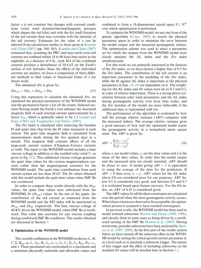
Dst data. In these events, the relative contributions fromeach current system due to the different inputs remainedroughly the same through the optimization process. Thesestorm events were characterized also by their classical nat-ure in that the onset, main phase and decay phase are dis-tinct. In another category (category II), the storms aremuch more dependent on the input coupling function used.For coupling functions that are significantly different fromeach other, the output Dst curves were different, and eachDst curve predicted a different level of geomagnetic activityover 6–8 h time scales. Here we have chosen to just use thestandard rectified solar wind input for our analysis.

Fig. 1 shows the comparison of Kyoto Dst and the Dst

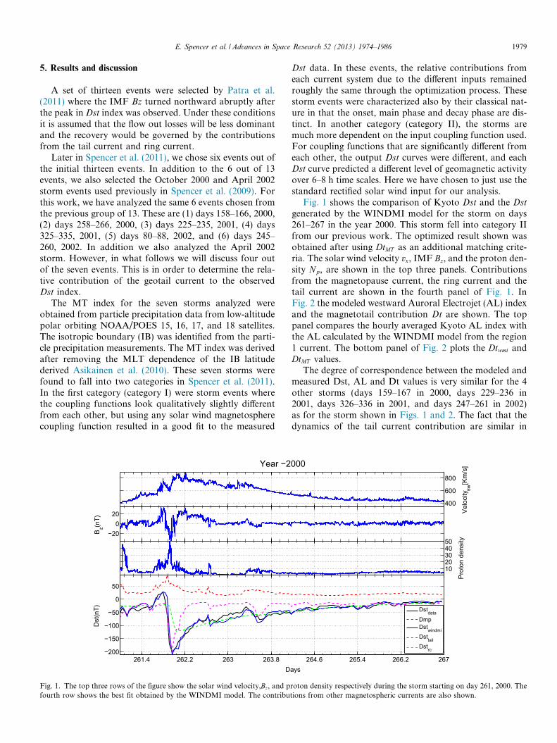
generated by the WINDMI model for the storm on days261–267 in the year 2000. This storm fell into category IIfrom our previous work. The optimized result shown wasobtained after using DtMT as an additional matching crite-ria. The solar wind velocity vx, IMF Bz, and the proton den-sity Np, are shown in the top three panels. Contributionsfrom the magnetopause current, the ring current and thetail current are shown in the fourth panel of Fig. 1. InFig. 2 the modeled westward Auroral Electrojet (AL) indexand the magnetotail contribution Dt are shown. The toppanel compares the hourly averaged Kyoto AL index withthe AL calculated by the WINDMI model from the region1 current. The bottom panel of Fig. 2 plots the Dtwmi andDtMT values.

The degree of correspondence between the modeled andmeasured Dst, AL and Dt values is very similar for the 4other storms (days 159–167 in 2000, days 229–236 in2001, days 326–336 in 2001, and days 247–261 in 2002)as for the storm shown in Figs. 1 and 2. The fact that thedynamics of the tail current contribution are similar in

400

600

800

000Ve

loci

tysw

[Km

/s]

1020304050

Prot

on d

ensi

ty

264.6 265.4 266.2 267ays

DstdataDmpDstwindmiDsttailDstrc

roton density respectively during the storm starting on day 261, 2000. Thetions from other magnetospheric currents are also shown.

262 263 264 265 266

200

400

600

800

1000

AL [n

T]

AL and Dt Comparison, Year 2000

ARV AL = 0.66

ALwindmiALdata

261 262 263 264 265 266 267

−150

−100

−50

0

Time [Days]

Dt [

nT]

DtwindmiDtMT

Fig. 2. The top panel shows the comparison of the AL index and the modeled values. The bottom panel of this figure shows the comparison between theDtMT values derived from the MT index and the Dtwmi for the storm starting on day 261, 2000.

1980 E. Spencer et al. / Advances in Space Research 52 (2013) 1974–1986

the two very different modeling approaches (MT andWINDMI based) corroborates that the tail current andits dynamics can be robustly monitored by the MT indexand that the WINDMI model is able to represent the over-all variation in the tail current as well. However, it seemsthat the good agreement between DtMT and Dtwmi is some-times broken during storm time substorms. We will nextdiscuss two such events.

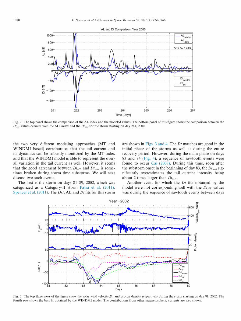
The first is the storm on days 81–89, 2002, which wascategorized as a Category-II storm Patra et al. (2011),Spencer et al. (2011). The Dst, AL and Dt fits for this storm

Year −2

−100

1020

B z(nT)

81 82 83 84 85−100

−50

0

50

Dst

(nT)

Days

Fig. 3. The top three rows of the figure show the solar wind velocity,Bz, and pfourth row shows the best fit obtained by the WINDMI model. The contribu

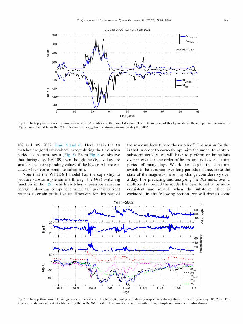
are shown in Figs. 3 and 4. The Dt matches are good in theinitial phase of the storms as well as during the entirerecovery period. However, during the main phase on days83 and 84 (Fig. 4), a sequence of sawtooth events werefound to occur Cai (2007). During this time, soon afterthe substorm onset in the beginning of day 83, the Dtwmi sig-nificantly overestimates the tail current intensity beingabout 2 times larger than DtMT .

Another event for which the Dt fits obtained by themodel were not corresponding well with the DtMT valueswas during the sequence of sawtooth events between days

400

600

002Ve

loci

tysw

[Km

/s]

20

40

60

Prot

on d

ensi

ty

86 87 88 89

DstdataDmpDstwindmiDsttailDstrc

roton density respectively during the storm starting on day 81, 2002. Thetions from other magnetospheric currents are also shown.

82 83 84 85 86 87 88

200

400

600

800

AL [n

T]

AL and Dt Comparison, Year 2002

ARV AL = 0.23

ALwindmiALdata

81 82 83 84 85 86 87 88 89

−40

−30

−20

−10

0

Time [Days]

Dt [

nT]

DtwindmiDtMT

Fig. 4. The top panel shows the comparison of the AL index and the modeled values. The bottom panel of this figure shows the comparison between theDtMT values derived from the MT index and the Dtwmi for the storm starting on day 81, 2002.

E. Spencer et al. / Advances in Space Research 52 (2013) 1974–1986 1981

108 and 109, 2002 (Figs. 5 and 6). Here, again the Dt

matches are good everywhere, except during the time whenperiodic substorms occur (Fig. 6). From Fig. 6 we observethat during days 108-109, even though the DtMT values aresmaller, the corresponding values of the Kyoto AL are ele-vated which corresponds to substorms.

Note that the WINDMI model has the capability toproduce substorm phenomena through the HðuÞ switchingfunction in Eq. (5), which switches a pressure relievingenergy unloading component when the geotail currentreaches a certain critical value. However, for this part of

Year −2

−20

0

20

B z(nT)

105.4 106.6 107.8 109 110

−100

−50

0

50

Dst

(nT)

Day

Fig. 5. The top three rows of the figure show the solar wind velocity,Bz, and pfourth row shows the best fit obtained by the WINDMI model. The contribu

the work we have turned the switch off. The reason for thisis that in order to correctly optimize the model to capturesubstorm activity, we will have to perform optimizationsover intervals in the order of hours, and not over a stormperiod of many days. We do not expect the substormswitch to be accurate over long periods of time, since thestate of the magnetosphere may change considerably overa day. For predicting and analyzing the Dst index over amultiple day period the model has been found to be moreconsistent and reliable when the substorm effect isexcluded. In the following section, we will discuss some

400500600

002Ve

loci

tysw

[Km

/s]

204060

Prot

on d

ensi

ty

.2 111.4 112.6 113.8 115s

DstdataDmpDstwindmiDsttailDstrc

roton density respectively during the storm starting on day 105, 2002. Thetions from other magnetospheric currents are also shown.

106 107 108 109 110 111 112 113 1140

200

400

600

800

1000

1200

AL [n

T]

AL and Dt Comparison, Year 2002

ARV AL = 0.34ALwindmiALdata

105 106 107 108 109 110 111 112 113 114 115−80

−60

−40

−20

Time [Days]

Dt [

nT] Dtwindmi

DtMT

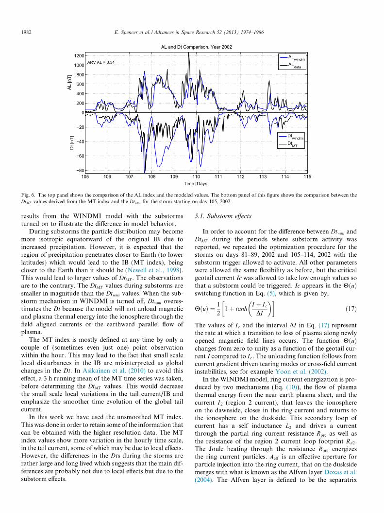
Fig. 6. The top panel shows the comparison of the AL index and the modeled values. The bottom panel of this figure shows the comparison between theDtMT values derived from the MT index and the Dtwmi for the storm starting on day 105, 2002.

1982 E. Spencer et al. / Advances in Space Research 52 (2013) 1974–1986

results from the WINDMI model with the substormsturned on to illustrate the difference in model behavior.

During substorms the particle distribution may becomemore isotropic equatorward of the original IB due toincreased precipitation. However, it is expected that theregion of precipitation penetrates closer to Earth (to lowerlatitudes) which would lead to the IB (MT index), beingcloser to the Earth than it should be (Newell et al., 1998).This would lead to larger values of DtMT . The observationsare to the contrary. The DtMT values during substorms aresmaller in magnitude than the Dtwmi values. When the sub-storm mechanism in WINDMI is turned off, Dtwmi overes-timates the Dt because the model will not unload magneticand plasma thermal energy into the ionosphere through thefield aligned currents or the earthward parallel flow ofplasma.

The MT index is mostly defined at any time by only acouple of (sometimes even just one) point observationwithin the hour. This may lead to the fact that small scalelocal disturbances in the IB are misinterpreted as globalchanges in the Dt. In Asikainen et al. (2010) to avoid thiseffect, a 3 h running mean of the MT time series was taken,before determining the DtMT values. This would decreasethe small scale local variations in the tail current/IB andemphasize the smoother time evolution of the global tailcurrent.

In this work we have used the unsmoothed MT index.This was done in order to retain some of the information thatcan be obtained with the higher resolution data. The MTindex values show more variation in the hourly time scale,in the tail current, some of which may be due to local effects.However, the differences in the Dts during the storms arerather large and long lived which suggests that the main dif-ferences are probably not due to local effects but due to thesubstorm effects.

5.1. Substorm effects

In order to account for the difference between Dtwmi andDtMT during the periods where substorm activity wasreported, we repeated the optimization procedure for thestorms on days 81–89, 2002 and 105–114, 2002 with thesubstorm trigger allowed to activate. All other parameterswere allowed the same flexibility as before, but the criticalgeotail current Ic was allowed to take low enough values sothat a substorm could be triggered. Ic appears in the HðuÞswitching function in Eq. (5), which is given by,

HðuÞ ¼ 1

21þ tanh

I � Ic

DI

� �� �ð17Þ

The values of Ic and the interval DI in Eq. (17) representthe rate at which a transition to loss of plasma along newlyopened magnetic field lines occurs. The function HðuÞchanges from zero to unity as a function of the geotail cur-rent I compared to Ic. The unloading function follows fromcurrent gradient driven tearing modes or cross-field currentinstabilities, see for example Yoon et al. (2002).

In the WINDMI model, ring current energization is pro-duced by two mechanisms (Eq. (10)), the flow of plasmathermal energy from the near earth plasma sheet, and thecurrent I2 (region 2 current), that leaves the ionosphereon the dawnside, closes in the ring current and returns tothe ionosphere on the duskside. This secondary loop ofcurrent has a self inductance L2 and drives a currentthrough the partial ring current resistance Rprc as well asthe resistance of the region 2 current loop footprint RA2.The Joule heating through the resistance Rprc energizesthe ring current particles. Aeff is an effective aperture forparticle injection into the ring current, that on the dusksidemerges with what is known as the Alfven layer Doxas et al.(2004). The Alfven layer is defined to be the separatrix

0

200

400

600

800

1000

1200

Time [Days]

AL [n

T]

AL and Dt Comparison, Year 2002

ARV AL = 0.52

ALwindmiALdata

81 82 83 84 85 86 87 88 89−35

−30

−25

−20

−15

−10

−5

0

Time [Days]

Dt [

nT]

DtwindmiDtwindmi−optDtMT

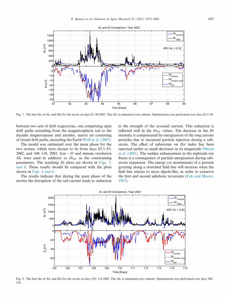
Fig. 7. The best fits of AL and Dts for the storm on days 81–89,2002. The AL is estimated every minute. Optimization was performed over days 82.5–84.

E. Spencer et al. / Advances in Space Research 52 (2013) 1974–1986 1983

between two sets of drift trajectories, one comprising opendrift paths extending from the magnetospheric tail to thedayside magnetopause and another, nearer set consistingof closed drift paths, encircling the Earth Wolf et al. (2007).

The model was optimized over the main phase for thetwo storms, which were chosen to be from days 82.5–85,2002, and 108–110, 2002. Sym� H and minute resolutionAL were used in addition to DtMT as the constrainingparameters. The resulting Dt plots are shown in Figs. 7,and 8. These results should be compared with the plotsshown in Figs. 4 and 6.

The results indicate that during the main phase of thestorms the disruption of the tail current leads to reduction

106 107 108 109

0

500

1000

1500

2000

Time

AL [n

T]

AL and Dt Com

105 106 107 108 109

−60

−40

−20

0

Time

Dt [n

T]

Fig. 8. The best fits of AL and Dts for the storm on days 105–115,2002. The A110.

in the strength of the crosstail current. This reduction isreflected well in the DtMT values. The decrease in the Dt

intensity is compensated by energization of the ring currentparticles due to increased particle injection during a sub-storm. The effect of substorms on Dst index has beenreported earlier as small decreases in its magnitude Ohtaniet al. (2001). The sudden enhancement in the nightside ionfluxes is a consequence of particle energization during sub-storm expansion. The energy (or momentum) of a particlegyrating along a stretched field line will increase when thefield line relaxes to more dipole-like, in order to conservethe first and second adiabatic invariants (Fok and Moore,1997).

110 111 112 113 114 [Days]

parison, Year 2002

ARV AL = 0.83

ALwindmiALdata

110 111 112 113 114 115 [Days]

DtwindmiDtwindmi−optDtMT

L is estimated every minute. Optimization was performed over days 108–

1984 E. Spencer et al. / Advances in Space Research 52 (2013) 1974–1986

But the enhanced inductive electric field during a sub-storm alone is not completely effective in energizing thering current. Sanchez et al. (1993) propose that, dipolariza-tion and accompanying current disruption cause ionswithin the reconfiguration region to be prevented from fur-ther earthward penetration, thus creating a temporary voidof plasma sheet particles in the inner edge of the plasmasheet. This could lead to lower enhancement of the ringcurrent particles during a substorm.

In our simulations, the optimization procedure makesthe energy input due to I2

2Rprc into the ring current duringsubstorms become dominant. The pVAeff energy inputbecomes small because the thermal pressure decreases sub-stantially in the plasma sheet when a substorm is triggered(Eq. (10)). Whether this is accurate can only be determinedby means of another measurement constraint imposed onthe model. We will address this issue in future modelingwork.

6. Conclusion

In this work we have used the MT-index, which is anindicator of the ion-isotropic boundary location, to con-strain the WINDMI model geotail current. The best fitWINDMI values were compared with the magnetic distur-bance estimated on the surface of the Earth due to thestrength of the tail current. The magnetotail current contri-bution to the Dst index as calculated by the WINDMImodel has a very good correlation with the values calcu-lated from the empirical expression relating the MT indexto the ground perturbation due to geotail current.

The addition of this additional constraint on theWINDMI model makes the calculated magnetosphericcurrents more reliable. We observed that for most storms,the relative contribution from the geotail current and ringcurrent to the Dst index obtained from our earlier studiesare consistent with the present work. The most significantdifference was observed for the storms where periodic sub-storms were observed during the storm. During suchstorms the MT index and the resulting Dt values show asignificant drop in magnitude that is attributed to the cur-rent disruption during a substorm, leading to lowerstrength of the geotail current.

The WINDMI model is able to confirm this observationwhen the substorms are triggered in the model. The corre-sponding drop in contribution to the Dst/Sym� H indicesis compensated by the enhancement in the energization ofthe ring current due to the increased inductive E-field dur-ing a substorm dipolarization. The observed Sym� H cor-relates favorably with these substorm dynamics. This worksuggests that the contribution from tail current to groundperturbation is important.

More work needs to be done to confirm the exact mech-anism for the energization of the ring current during a sub-storm. The conditions that trigger a substorm in themagnetosphere is still an open question and further studiesare required. The combination of the right trigger condi-

tion as well as the correct energization mechanism for thering current will enable the WINDMI model to reproducethe Dst index more realistically.

References

Aguado, J., Cid, C., Saiz, E., Cerrato, Y., 2010. Hyperbolic decay ofthe dst index during the recovery phase of intense geomagneticstorms. J. Geophys. Res. 115 (A07220), http://dx.doi.org/10.1029/2009JA014658.

Alexeev, I.I., Belenkaya, E.S., Kalegaev, V.V., Feldstein, Y.I., Grafe, A.,1996. Magnetic storms and magnetotail currents. J. Geophys. Res. 101(A4), 7737–7747.

Asikainen, T., Maliniemi, V., Mursula, K., 2010. Modeling the contribu-tions of ring, tail, and magnetopause currents to the corrected dstindex. JGR 115 (A12203), http://dx.doi.org/10.1029/2010JA015774.

Bala, R., Reiff, P.H., Landivar, J.E., 2009. Real-time prediction ofmagnetospheric activity using the boyle index. SW 7 (S04003), http://dx.doi.org/10.1029/2008SW000407.

Burton, R.K., McPherron, R.L., Russell, C.T., 1975. An empiricalrelationship between interplanetary conditions and dst. JGR 80 (31),4204–4214.

Buzulukova, N., Fok, M., Pulkkinen, A., Kuznetsova, M., Moore, T.E.,Glocer, A., Brandt, P.C., To? th, G., Rasta? tter, L., 2010. Dynamicsof ring current and electric fields in the inner magnetosphere duringdisturbed periods: Crcmbats-r-us coupled model. J. Geophys. Res. 115(A05210), http://dx.doi.org/10.1029/2009JA014621.

Cai, X. 2007. Investigation of global periodic sawtooth oscillationsobserved in energetic particle flux at geosynchronous orbit. Ph.D.thesis, University of Michigan, Ann Arbor, MI.

Chen, M., Schulz, M., Lyons, L., Gorney, D., 1993. Stormtime transportof ring current and radiation belt ions. J. Geophys. Res. 98 (A3), 3835–3849.

Coley, D.A., 2003. An Introduction to Genetic Algorithms for Scientistsand Engineers. World Scientific Publishing Co., Inc., Tokyo, Japan.

Dessler, A., Parker, E.N., 1959. Hydromagnetic theory of geomagneticstorms. J. Geophys. Res. 64, 2239–2259.

Donovan, E.F., Jackel, B.J., Voronkov, I., Sotirelis, T., Creutzberg, F.,Nicholson, N.A., 2003. Ground-based optical determination of the b2iboundary: a basis for an optical mt-index. J. Geophys. Res. 108 (A3,1115), 1147–1155.

Doxas, I., Horton, W., Lin, W., Seibert, S., Mithaiwala, M., 2004. Adynamical model for the coupled inner magnetosphere and tail. IEEETrans. Plasma Sci. 32 (4), 1443–1448.

Ebihara, Y., Ejiri, M., 2000. Simulation study on fundamental propertiesof the storm-time ring current. J. Geophys. Res. 105 (A7), 15843–15859.

Feldstein, Y.I., Dremukhina, L.A., 2000. On the two-phase decay of thedst-variation. JGR 27 (17), 2813–2816.

Fok, M.C., Moore, T.E., 1997. Ring current modeling in a realisticmagnetic field configuration. Geophys. Res. Lett. 24 (14), 1775–1778.

Fok, M.C., Kozyra, J.U., Nagy, A.F., 1991. Lifetime of ring currentparticles due to coulomb collisions in the plasmasphere. J. Geophys.Res. 96 (A5), 7861–7867.

Fok, M.C., Kozyra, J.U., Nagy, A.F., Rasmussen, C.E., Khazanov, G.V.,1993. Decay of equatorial ring current ions and associated aeronom-ical consequence. J. Geophys. Res. 98 (A11), 19381–19393.

Fok, M.C., Wolf, R.A., Spiro, R.W., Moore, T.E., 2001. Comprehensivecomputational model of earth’s ring current. J. Geophys. Res. 106(A5), 8417–8424.

Ganushkina, N.Y., Pulkkinen, T.I., Kubyshkina, M.V., Singer, H.J.,Russell, C.T., 2004. Long-term evolution of magnetospheric currentsystems during storms. Ann. Geophys. 22, 1317–1334.

Ganushkina, N.Y., Pulkkinen, T., Fritz, T., 2005a. Role of substorm-associated impulsive electric fields in the ring current developmentduring storms. Ann. Geophys. 23, 579–591.

E. Spencer et al. / Advances in Space Research 52 (2013) 1974–1986 1985

Ganushkina, N.Y., Pulkkinen, T.I., Kubyshkina, M.V., Sergeev, V.A.,Lvova, E.A., Yahnina, T.A., Yahnin, A.G., Fritz, T., 2005b. Protonisotropy boundaries as measured on mid and low-altitude satellites.Ann. Geophys. 23, 1839–1847.

Ganushkina, N.Y., Liemohn, M.W., Pulkkinen, T.I., 2012. Storm-timering current: model-dependent results. Ann. Geophys. 30, 177–202.

Horton, W., Doxas, I., 1996. A low-dimensional energy-conserving statespace model for substorm dynamics. J. Geophys. Res. 101 (A12),27223–27237.

Horton, W., Doxas, I., 1998. A low-dimensional dynamical model for thesolar wind driven geotail-ionosphere system. J. Geophys. Res. 103(A3), 4561–4572.

Horton, W., Weigel, R.S., Vassiliadis, D., Doxas, I., 2003. Substormclassification with the windmi model. Nonlinear Processes Geophys.10, 363–371.

Jayachandran, P.T., Donovan, E.F., MacDougall, J.W., Moorcroft, D.R.,Maurice, J.S., Prikryl, P., 2002a. Superdarn e-region backscatterboundary in the dusk-midnight sector tracer of equatorward boundaryof the auroral oval. Ann. Geophys. 20, 1899–1904.

Jayachandran, P.T., MacDougall, J.W., St-Maurice, J.-P., Moorcroft,D.R., Newell, P.T., Prikryl, P., 2002b. Coincidence of the ionprecipitation boundary with the hf e region backscatter boundary inthe dusk-midnight sector of the auroral oval. Geophys. Res. Lett. 29(8, 1256), 1147–1155.

Jordanova, V.K., Kozyra, J.U., Nagy, A.F., Khazanov, G.V., 1997.Kinetic model of the ring current-atmosphere interactions. J. Geophys.Res. 102 (A7), 14279–14291.

Jordanova, V.K., Farrugia, C.J., Thorne, R.M., Khazanov, G.V., Reeves,G.D., Thomsen, M.F., 2001. Modeling ring current proton precipita-tion by electromagnetic ion cyclotron waves during the may 1416,1997, storm. J. Geophys. Res. 106 (A1), 7–22.

Jordanova, V.K., Kistler, L.M., Thomsen, M.F., Mouikis, C.G., 2003.Effects of plasma sheet variability on the fast initial ring current decay.Geophys. Res. Lett. 30 (6, 1311). http://dx.doi.org/10.1029/2002GL016576.

Kalegaev, V., Makarenkov, E., 2008. Relative importance of ring and tailcurrents to dst under extremely disturbed conditions. J. Atmos. Sol.Terr. Phys. 70, 519–525.

Kamide, Y., Chian, A. (Eds.), 2007. Handbook of the Solar-TerrestrialEnvironment. Springer Verlag.

Konradi, A., Semar, C.L., Fritz, T.A., 1975. Substorm-injected protonsand electrons and the injection boundary model. J. Geophys. Res. 80(4), 543–552.

Kozyra, J.U., Fok, M.C., Sanchez, E.R., Evans, D.S., Hamilton, D.,Nagy, A.F., 1998. The role of precipitation looses in producing therapid early recovery phase of the great magnetic storm of february1986. J. Geophys. Res. 103 (A4), 6801–6814.

Kubyshkina, M., Sergeev, V., Tsyganenko, N., Angelopoulos, V., Runov,A., Singer, H., Glassmeier, K.H., Auster, H.U., Baumjohann, W.,2009. Toward adapted time-dependent magnetospheric models: asimple approach based on tuning the standard model. J. Geophys. Res.114 (A00C21), http://dx.doi.org/10.1029/2008JA013547.

Langel, R.A., Estes, R.H., 1985. Large-scale, near-field magnetic fieldsfrom external sources and the corresponding induced internal field. J.Geophys. Res. 90 (B3), 2487–2494.

Liemohn, M.W., Kozyra, J.U., 2005. Testing the hypothesis that chargeexchange can cause a two-phase decay. In: The Inner Magnetosphere:Physics and Modeling. Vol. 155 of Geophysical Monograph Series.American Geophysical Union, Washington DC, pp. 211–225, http://dx.doi.org/10.1029/GM155.

Liemohn, M.W., Kozyra, J.U., Clauer, C.R., Ridley, A.J., 2001. Com-putational analysis of the near-earth magnetospheric current systemduring two-phase decay storms. JGR 106 (A12), 29531–29542.

Maltsev, Y., 2004. Points of controversy in the study of magnetic storms.Space Sci. Rev. 110, 227–267.

Maltsev, Y.P., Arykov, A.A., Belova, E.G., Gvozdevskay, B.B., Safarga-leev, V.V., 1996. Magnetic flux redistribution in the storm timemagnetosphere. J. Geophys. Res. 101 (A4), 7697–7704.

Mattinen, M. 2010. Modeling and forecasting of local geomagneticactivity. Master’s thesis, AALTO UNIVERSITY, School of Scienceand Technology, Faculty of Information and Natural Sciences,Helsinki.

Meurant, M., Gerard, J.-C., Blockx, C., Spanswick, E., Donovan, E.F.,Coumans, B.H.V., Connors, M., 2007. El?a possible indicator tomonitor the magnetic field stretching at global scale during substormexpansive phase: statistical study. J. Geophys. Res. 112 (A105222),http://dx.doi.org/10.1029/2006JA012126.

Mithaiwala, M.J., Horton, W., 2005. Substorm injections producesufficient electron energization to account for mev flux enhancementsfollowing some storms. J. Geophys. Res. 110 (A07224), 363–371.

Mursula, K., Karinen, A., 2005. Explaining and correcting the excessivesemiannual variation in the dst index. Geophys. Res. Lett. 32(L14107), http://dx.doi.org/10.1029/2005GL023132.

Newell, P.T., Feldstein, Y.I., Galperin, Y.I., Meng, C.-I., 1996. Morphol-ogy of nightside precipitation. J. Geophys. Res. 101 (A5), 10737–10748.

Newell, P.T., Sergeev, V.A., Bikkuzina, G.R., Wing, S., 1998. Character-izing the state of the magnetosphere: testing the ion precipitationmaxima latitude (b2i) and the ion isotropy boundary. J. Geophys. Res.103 (A3), 4739–4745.

Newell, P., Sotirelis, T., Skura, J.P., Meng, C.I., Lyatsky, W., 2002.Ultraviolet insolation drives seasonal and diurnal space weathervariations. J. Geophys. Res. 107 (A10), 1305. http://dx.doi.org/10.1029/2001JA000296.

Newell, P., Sorelis, T., Liou, K., Meng, C.-I., Rich, F., 2007. A nearlyuniversal solar wind-magnetosphere coupling function inferred from10 magnetospheric state variables. J. Geophys. Res. 112 (A01206),http://dx.doi.org/10.1029/2006JA012015.

O’Brien, T.P., McPherron, R.L., 2000. An empirical phase space analysisof ring current dynamics: solar wind control of injection and decay. J.Geophys. Res. 105 (A4).

Ohtani, S., Nose, M., Rostoker, G., Singer, H., Lui, A.T.Y., Nakamura,M., 2001. Storm-substorm relationship: contribution of the tail currentto dst. J. Geophys. Res. 106 (A10), 21199–21209.

Patra, S., Spencer, E., Horton, W., Sojka, J., 2011. Study of dst/ringcurrent recovery times using the windmi model. J. Geophys. Res. 116(A02212), http://dx.doi.org/10.1029/2010JA015824.

Reiff, P.H., Luhmann, J.G., 1986. Solar wind control of the polar-capvoltage. In: Kamide, Y., Slavin, J.A. (Eds.), Solar Wind-Magneto-sphere Coupling. Terra Sci., Tokyo, pp. 453–476.

Sanchez, E.R., Mauk, B.H., Newell, P.T., Meng, C., 1993. Low-altitudeobservations of the evolution of substorm injection boundaries. J.Geophys. Res. 98 (A4), 5815–5838.

Sckopke, N., 1966. A general relation between the energy of trappedparticles and the disturbance field near the Earth. J. Geophys. Res. 71,3125.

Sergeev, V., Gvozdevsky, B., 1995. Mt-index: a possible new index tocharacterize the magnetic configuration of magnetotail. Ann. Geo-phys. 13, 1093–1103.

Sergeev, V.A., Sazhina, E.M., Tsyganenko, N.A., Lundblad, J.A.,Soraas, F., 1983. Pitch angle scattering of energetic protons in themagnetotail current sheet as the dominant source of their isotropicprecipitation into the nightside ionosphere. Planet. Space Sci. 31(10), 1147–1155.

Sergeev, V.A., Malkov, M., Mursula, K., 1993. Testing the isotropicboundary algorithm method to evaluate the magnetic field configura-tion in the tail. J. Geophys. Res. 98 (A5), 7609–7620.

Sergeev, V.A., Pulkkinen, T.I., Pellinen, R.J., Tsyganenko, N.A., 1994.Hybrid state of the tail magnetic configuration during steady convec-tion events. J. Geophys. Res. 99 (A12), 23571–23582.

Spencer, E., Horton, W., Mays, L., Doxas, I., Kozyra, J., 2007. Analysisof the 3–7 October 2000 and 15–24 April 2002 geomagnetic stormswith an optimized nonlinear dynamical model. J. Geophys. Res. 112962 (A04S90), http://dx.doi.org/10.1029/2006JA012019.

Spencer, E., Rao, A., Horton, W., Mays, M.L., 2009. Evaluation of solarwind-magnetosphere coupling functions during geomagnetic storms

1986 E. Spencer et al. / Advances in Space Research 52 (2013) 1974–1986

with the windmi model. J. Geophys. Res. 114 (A02206), http://dx.doi.org/10.1029/2008JA013530.

Spencer, E., Kasturi, P., Patra, S., Horton, W., Mays, M.L., 2011.Influence of solar wind magnetosphere coupling functions on the dstindex. J. Geophys. Res. 116 (A12235), http://dx.doi.org/10.1029/2011JA016780.

Takahashi, S., Iyemori, T., Takeda, M., 1990. A simulation of the stormtime ring current. Planet. Space Sci. 38 (9), 1133–1141.

Temerin, M., Li, X., 2002. A new model for the prediction of dst on thebasis of the solar wind. JGR 107 (A12), http://dx.doi.org/10.1029/2001JA007532.

Temerin, M., Li, X., 2006. Dst model for 19952002. JGR 111 (A04221),http://dx.doi.org/10.1029/2005JA011257.

Tsyganenko, N.A., Sitnov, M.I., 2005. Modeling the dynamics of the innermagnetosphere during strong geomagnetic storms. JGR 110 (A3208),http://dx.doi.org/10.1029/2004JA010798.

Turner, N.E., Baker, D.N., Pulkkinen, T.I., McPherron, R.L., 2000.Evaluation of the tail current contribution to dst. J. Geophys. Res. 105(A02212), 5431–5439.

Walt, M., Voss, H.D., 2001. Losses of ring current ions by strong pitchangle scattering. Geophys. Res. Lett. 28 (20), 3839–3841.

Wolf, R., Spiro, R., Sazykin, S., Toffoletto, F., 2007. How the earth’sinner magnetosphere works: an evolving picture. J. Atmos. Sol. Terr.Phys. 69, 288–302.

Yoon, P., Lui, A., Sitnov, M., 2002. Generalized lower-hybrid drift instabilitiesin current sheet equilibrium. Phys. Plasma. 9 (5), 1526–1538.