1

DCT and DST Filtering with Sparse Graph OperatorsKeng-Shih Lu, Member, IEEE, Antonio Ortega, Fellow, IEEE, Debargha Mukherjee, Senior Member, IEEE, and Yue Chen

Abstract—Graph filtering is a fundamental tool in graph signalprocessing. Polynomial graph filters (PGFs), defined as polynomialsof a fundamental graph operator, can be implemented in the vertexdomain, and usually have a lower complexity than frequency domainfilter implementations. In this paper, we focus on the design of filtersfor graphs with graph Fourier transform (GFT) corresponding to adiscrete trigonometric transform (DTT), i.e., one of 8 types of discretecosine transforms (DCT) and 8 discrete sine transforms (DST). In thiscase, we show that multiple sparse graph operators can be identified,which allows us to propose a generalization of PGF design: multivariatepolynomial graph filter (MPGF). First, for the widely used DCT-II (type-2 DCT), we characterize a set of sparse graph operators that share theDCT-II matrix as their common eigenvector matrix. This set containsthe well-known connected line graph. These sparse operators can beviewed as graph filters operating in the DCT domain, which allows usto approximate any DCT graph filter by a MPGF, leading to a designwith more degrees of freedom than the conventional PGF approach.Then, we extend those results to all of the 16 DTTs as well as their 2Dversions, and show how their associated sets of multiple graph operatorscan be determined. We demonstrate experimentally that ideal low-passand exponential DCT/DST filters can be approximated with higheraccuracy with similar runtime complexity. Finally, we apply our methodto transform-type selection in a video codec, AV1, where we demonstratesignificant encoding time savings, with a negligible compression loss.

Index Terms—graph filtering, discrete cosine transform, asymmetricdiscrete sine transform, graph Fourier transform

I. INTRODUCTION

Graph signal processing (GSP) [1]–[3] extends classical signalprocessing concepts to data living on irregular domains. In GSP, thedata domain is represented by a graph, and the measured data is calledgraph signal, where each signal sample corresponds to a graph vertex,and relations between samples are captured by the graph edges.Filtering, where frequency components of a signal are attenuated oramplified, is a fundamental operation in signal processing. Similarto conventional filters in digital signal processing, which manipulatesignals in Fourier domain, a graph filter can be characterized by afrequency response that indicates how much the filter amplifies eachgraph frequency component. This notion of frequency selection leadsto various applications, including graph signal denoising [4]–[6],classification [7] and clustering [8], and graph convolutional neuralnetworks [9], [10].

For an undirected graph, a frequency domain graph filter operationy = Hx with input signal x and filter matrix

H = Φ ⋅ h(Λ) ⋅Φ⊺, h(Λ) ∶= diag(h(λ1),⋯, h(λN)) (1)

involves a forward graph Fourier transform (GFT) Φ⊺, a frequencyselective scaling operation h(Λ), and an inverse GFT Φ. However, asfast GFT algorithms are only known for graphs with certain structuralproperties [11], the GFT can introduce a high computational overheadwhen the graph is arbitrary. To address this issue, graph filters can

K.-S. Lu, D. Mukherjee and Y. Chen are with Google, MountainView, CA 94043, USA (email: kslu@google.com; debargha@google.com;yuec@google.com). Most of this work has been done while K.-S. Lu wasa PhD student at USC.

A. Ortega is with the Department of Electrical and Computer Engineering,University of Southern California, Los Angeles, CA 90089, USA (email:ortega@sipi.usc.edu).

be implemented with polynomial operations in vertex domain:

H =K

∑k=0

gkZk, with Z0

= I, (2)

where the gk’s are coefficients and Z is called the graph shift oper-ator, fundamental graph operator, or graph operator for short. Withthis expression, graph filtering can be applied in the vertex (sample)domain via y = Hx, which does not require GFT computations. Agraph filter in the form of (2) is usually called an FIR graph filter[12], [13] as it can be viewed as an analogy to conventional FIR filterswith order K, which are polynomials of the delay z. In this paper,we call the filters defined in (2) polynomial graph filters (PGFs).

Various methods for designing vertex domain graph filters givena desired frequency response have been studied in the literature.Least squares design of polynomial filters given a target frequencyresponse was introduced in [14]–[16]. The recurrence relations ofChebyshev polynomials provide computational benefits in distributedfilter implementations as shown in [17], [18]. In [19] an extensionof graph filter operations to a node-variant setting is proposed, alongwith polynomial approximation approaches using convex optimiza-tion. Autoregressive moving average (ARMA) graph filters, whosefrequency responses are characterized by rational polynomials, havebeen investigated in [12], [20] in both static and time-varying settings.Design strategies of ARMA filters are further studied in [21], whichprovides comparisons to PGFs. Furthermore, in [13], state-of-the-artfiltering methods have been extended to an edge-variant setting. Allthese methods are based on using a single graph operator Z.

The possibility of using multiple operators was first observedin [22]. Multiple graph operators Z = {Z(1),Z(2), . . . ,Z(m)} thatare jointly diagonalizable (i.e., have a common eigenbasis) can beobtained for both cycle graphs [22] and line graphs [23]. Essentially,those operators are by themselves graph filter matrices with differentfrequency responses. Thus, unlike (2), which is a polynomial of asingle operator, we can design graph filters of the form:

HZ,K = pK(Z(1),Z(2), . . . ,Z(m)), (3)

where pK(⋅) stands for a multivariate polynomial with degree K andarbitrary coefficients. Given the graph filter expression (3), iterativealgorithms for filter implementation have been recently studied in[24]. Since H{Z},K = pK(Z) reduces to (2), the form (3) is ageneralization of the PGF expression. We refer to (3) as multivariatepolynomial graph filter (MPGF).

In this paper, we focus on filtering operations based on the well-known discrete cosine transform (DCT) and discrete sine transform(DST) [25], as well as their extension to all discrete trigonometrictransforms (DTTs), i.e., 8 types of DCTs and 8 types of DSTs [26].All DTTs are GFTs associated with uniform line graphs [25], [26].DTT filters are based on the following operations: 1) computingthe DTT of the input signal, 2) scaling each of the computed DTTcoefficients, and 3) performing the inverse DTT. In particular, DCTfilters [27] have long been studied and are typically implementedusing forward and inverse DCT. As an alternative, we propose graph-based approaches to design and implement DTT filters. The mainadvantage of graph based approaches is that they do not require theDTT and inverse DTT steps, and instead can be applied directly inthe signal domain, using suitable graph operators. This allows us to

arX

iv:2

103.

1152

9v1

[ee

ss.S

P] 2

2 M

ar 2

021

2

define graph filtering approaches for all DTT filters, with applicationsincluding image resizing [28], biomedical signal processing [29],medical imaging [30], and video coding [31].

Our work studies the design of efficient sample domain (graphvertex domain) graph filters, with particular focus on DTT filters.Specifically, for GFTs corresponding to any of the 16 DTTs, wederive a family Z of sparse graph operators with closed form expres-sions, which can be used in addition to the graph operator obtainedfrom the well-known line graph model [26]. In this way, efficientDTT filters can be obtained using PGF and MPGF design approaches,yielding a lower complexity than a DTT filter implementation in thetransform domain. Our main contributions are summarized as follows:

1) We introduce multiple sparse graph operators specific to DTTsand allowing fast MPGF implementations. These sparse oper-ators are DTT filters, which are special cases of graphs filters,but have not been considered in the general graph filteringliterature [12], [13], [18]–[21]. While [25] and [26] establish theconnection between DTTs and line graphs, our proposed sparsegraph operators for DTTs, which are no longer restricted to beline graphs, had not been studied in the literature.

2) We introduce novel DTT filter design methods for graph vertexdomain implementation. While in related work [26], [32], [33],DTT filtering is typically performed in the transform domainusing convolution-multiplication properties, we introduce sam-ple domain DTT filter implementations based on PGF andMPGF designs, and show that our designs with low degreepolynomials lead to faster implementations as compared tothose designs that require forward and inverse DTTs, especiallyin cases where DTT size is large.

3) In addition to the well-known least squares graph filter design,we propose a novel minimax design approach for both PGFsand MPGFs, which optimally minimizes the approximationerror in terms of maximum absolute error in the graph fre-quencies.

4) We provide novel insights on MPGF designs by demonstratingthat using multiple operators leads to more efficient implemen-tations, as compared to conventional PGF designs, for DTTfilters with frequency responses that are non-smooth (e.g., ideallow-pass filters) or non-monotonic (e.g., bandpass filters).

5) We demonstrate experimentally the benefits of sparse DTToperators in image and video compression applications. Inaddition to filter operation, our approach can also be usedto evaluate the transform domain weighted energy given bythe Laplacian quadratic form, which has been used for rate-distortion optimization in the context of image and video coding[34], [35]. Following our recent work [23], we implement theproposed method in AV1, a real-world codec, where our methodprovides a speedup in the transform type search procedure.

We highlight that, while [24] studies MPGFs with a focus ondistributed filter implementations, it does not investigate designapproaches of MPGFs or how sparse operators for generic graphscan be obtained other than cycle and Cartesian product graphs. Ourwork complements the study in [24] by considering 1) the case whereGFT is a DTT, which corresponds to various line graphs, and 2)techniques to design MPGFs. In addition, the work presented in thispaper is a more general framework than our prior work in [23], sincethe Laplacian quadratic form operation used in [23] can be viewedas a special case of graph filtering operation. Furthermore, while ourwork in [23] was restricted to DCT/ADST, in this paper we haveextended these ideas to all DTTs.

The rest of this paper is organized as follows. We review graphfiltering concepts and some relevant properties of DTTs in Section II.

In Section III, we consider sparse operators for DTTs that can beobtained by extending well-known properties of DTTs. We alsoextend the results to 2D DTTs and provide some remarks on sparseoperators for general graphs. Section IV introduces PGF and MPGFdesign approaches using least squares and minimax criteria. Anefficient filter design for Laplacian quadratic form approximationis also presented. Experimental results are shown in Section V todemonstrate the effectiveness of our methods in graph filter designas well as applications in video coding. Conclusions are given inSection VI.

II. PRELIMINARIES

We start by reviewing relevant concepts in graph signal processingand DTTs. In what follows, entries in a matrix that are not displayedare meant to be zero. Thus, the order-reversal permutation matrix is:

J =

⎛⎜⎜⎜⎝

11

⋰

1

⎞⎟⎟⎟⎠

,

which satisfies J⊺ = J and JJ = I, where the transpose of matrix Ais denoted as A⊺. The pseudo-inverse of A is written as A†.

A. Graph Fourier Transforms

Let G(V,E ,W) be an undirected graph with N nodes and letx be a length-N graph signal associated to G. Each node of Gcorresponds to an entry of x, and each edge eij ∈ E describes theinter-sample relation between nodes i and j. The (i, j) entry of theweight matrix, wi,j , is the weight of the edge eij , and θi ∶= wi,i isthe weight of the self-loop on node i. Defining Θ = diag(θ1, . . . , θN)

and D = diag(d1, . . . , dN) as diagonal matrices of self-loop weightsand node degrees, di = ∑Nj=1wi,j , respectively, the unnormalized andnormalized graph Laplacian matrices are

L = D −W +Θ, L = D−1/2LD−1/2. (4)

In what follows, unless stated otherwise, we refer to the unnormalizedversion, L, as the graph Laplacian. All graphs we consider areassumed to be undirected.

The graph Fourier transform (GFT) is obtained from the eigen-decomposition of the graph Laplacian, L = ΦΛΦ⊺, with eigenvaluesλ1 ≤ ⋯ ≤ λN in ascending order. The vector of GFT coefficients forgraph signal x is x = Φ⊺x. We note that the variation of signal x onthe graph can be measured by the Laplacian quadratic form:

x⊺Lx = ∑(i,j)∈E

wi,j(xi − xj)2+

N

∑k=1

θkx2k. (5)

The columns of Φ, φ1, . . . ,φN form an orthogonal basis and eachof them can be viewed as a graph signal with variation equalto the associated eigenvalues λ1, . . . , λN , which are called graphfrequencies.

B. Graph Filters

We consider a 1-hop graph operator Z, which could be theadjacency matrix or one of the Laplacian matrices. For a givensignal x, y = Zx defines an operation where the output at eachnode is a function of values at its 1-hop neighbors (e.g., whenZ = A, y(i) = ∑j∈N(i) x(j), where N (i) is the set of nodes thatare neighbors of i). Furthermore, it can be shown that y = ZKx isa K-hop operation, and thus for a degree-K polynomial of Z, asin (2), the output at node i depends on its K-hop neighbors. Theoperation in (2) is thus called a graph filter, an FIR graph filter, or

3

(a) (b)

Fig. 1. Graphs associated to (a) DCT-II, (b) DST-IV (ADST).

a polynomial graph filter (PGF). In what follows, we refer to Z asgraph operator for short1. For the rest of this paper, we choose Z = Lor define Z as a matrix with the same eigenbasis as L, e.g., Z couldbe a polynomial of L such as Z = 2I −L.

The matrix Φ of eigenvectors of Z = L is also the eigenvectormatrix of any polynomial H in the form of (2). The eigenvalueh(λj) of H associated to φj is called the frequency response of λj .Note that with y = Hx, in the GFT domain we have y = h(Λ)x,meaning that the filter operator scales the signal component withλj frequency by h(λj) in the GFT domain. We also note that (1)generalizes the notion of digital filter: when Φ is the discrete Fouriertransform (DFT) matrix, H reduces to the classical Fourier filter [15].Given a desired graph frequency response h = (h1, . . . , hN)

⊺, itsassociated polynomial coefficients in (2) can be obtained by solvinga least squares minimization problem [15]:

g = argming

∣∣h −Ψg∣∣2, where Ψ =⎛⎜⎝

1 λ1 . . . λK1⋮ ⋮ ⋮ ⋮

1 λN . . . λKN

⎞⎟⎠, (6)

with λj being the j-th eigenvalue of Z. The PGF operation y = Hxcan be implemented efficiently by computing: 1) t(0) = gKx, 2)t(i) = Zt(i−1) + gK−ix, and 3) y = t(K). This algorithm does notrequire GFT computation, and its complexity depends on the degreeK and how sparse Z is (with lower complexity for sparser Z).

C. Discrete Cosine and Sine Transforms

The discrete cosine transform (DCT) and discrete sine transform(DST) are orthogonal transforms that operate on a finite vector, withbasis functions derived from cosines and sines, respectively. Discretetrigonometric transforms (DTTs) comprise eight types of DCT andeight types of DST, which are defined depending on how samplesare taken from continuous cosine and sine functions [26], [36]. Wedenote them by DCT-I to DCT-VIII, and DST-I to DST-VIII, and listtheir forms in Table I.

DCT and ADST are widely used in image and video coding. Inthis paper, we refer the terms “DCT” and “ADST” to DCT-II andDST-IV2, respectively, unless stated otherwise. For j = 1, . . . ,N andk = 1, . . . ,N , we denote the k-th element of the j-th length-N DCTand ADST functions as

DCT-II: uj(k) =

√2

Ncj cos

(j − 1)(k − 12)π

N, (7)

DST-IV: vj(k) =

√2

Nsin

(j − 12)(k − 1

2)π

N. (8)

with normalization constant cj being 1/√2 for j = 1 and 1 otherwise.

If those basis functions are written in vector form uj ,vj ∈ RN , it

1In the literature, Z is often called graph shift operator [1], [12], [19], [22].Here, we simply call it graph operator, since its properties are different fromshift in conventional signal processing, which is always reversible, while thegraph operator Z, in most cases, is not.

2DST-VII was shown to optimally decorrelate intra residual pixels under aGaussian Markov model [37], [38], but its variant DST-IV is amenable to fastimplementations while experimentally achieving a similar coding efficiency[39]. In this paper, we refer to DST-IV as ADST, as in the AV1 codec [40].

was pointed out in [25] that the uj are eigenvectors of the Laplacianmatrix LD, and in [26] that vj are eigenvectors of LA, with

LD =

⎛

⎜⎜⎜⎜⎜

⎝

1 −1−1 2 −1

⋱ ⋱ ⋱

−1 2 −1−1 1

⎞

⎟⎟⎟⎟⎟

⎠

, LA =

⎛

⎜⎜⎜⎜⎜

⎝

3 −1−1 2 −1

⋱ ⋱ ⋱

−1 2 −1−1 1

⎞

⎟⎟⎟⎟⎟

⎠

. (9)

This means that the DCT and ADST are GFTs corresponding toLaplacian matrices LD and LA, respectively. Their associated graphsGD and GA with N = 6 are shown in Figs. 1(a) and (b). The eigenval-ues of LD corresponding to uj are ωj = 2− 2 cos((j − 1)π/N), andthose of LA corresponding to vj are δj = 2 − 2 cos((j − 1/2)π/N).

III. SPARSE DCT AND DST OPERATORS

Classical PGFs can be extended to MPGFs [24] if multiple graphoperators are available [22]. Let L = ΦΛΦ⊺ be a Laplacian with GFTΦ and assume we have a series of graph operators Z = {Z(k)}Mk=1that share the same eigenvectors as L, but with different eigenvalues:

Z(k) = ΦΛ(k)Φ⊺, Λ(k) = diag(λ(k)) = diag(λ(k)1 , . . . , λ(k)N ),

where λ(k) = (λ(k)1 , . . . , λ

(k)N )

⊺ denotes the vector of eigenvalues ofZ(k). When the polynomial degree is K = 1 in (3), we have:

HZ,1 = g0I +M

∑m=1

gmZ(m), (10)

where gk are coefficients. When K = 2, we have

HZ,2 = g0I +M

∑m=1

gmZ(m)

+ gM+1Z(1)Z(1) + gM+2Z

(1)Z(2) + ⋅ ⋅ ⋅ + g2MZ(1)Z(M)

+ g2M+1Z(2)Z(2) + ⋅ ⋅ ⋅ + g3M−1Z

(2)Z(M)

+ . . .

+ g(M2+3M)/2Z(M)Z(M), (11)

where the terms Z(j)Z(i) with j > i are not required in (11) becauseall operators commute, i.e., Z(i)Z(j) = Z(j)Z(i). Expressions witha higher degree can be obtained with polynomial kernel expansion[41]. We also note that, since H{Z},K reduces to the form of H in(2), HZ,K is a generalization of PGF and thus provides more degreesof freedom for the filter design procedure.

As pointed out in the introduction, DTT filters are essentially graphfilters. This means that they can be implemented with PGFs as in (2),without applying any forward or inverse DTT. Next, we will go onestep further by introducing multiple sparse operators for each DTT,which allows the implementation of DTT filters using MPGFs.

The use of polynomial (2) to perform filtering in the vertex domain,rather in the frequency domain, is advantageous only if the operatoris sparse. In this section, our main goal is to show that multiplesparse operators can be found for DTTs. First, the result of [25] willbe generalized in Sec. III-A to derive multiple sparse operators froma single operator for DCT-II. A toy example for those operators isprovided in Sec. III-B. Then, in Sec. III-C, we further show that, inaddition to DCT-II, operators can be derived for all 16 DTTs basedon the approach in Sec. III-A. Finally, sparse operators associated to2D DTTs are presented in Sec. III-D.

A. Sparse DCT-II Operators

Let uj denote the DCT basis vector with entries from (7) andlet LD be the Laplacian of a uniform line graph, (9). The followingproposition from [25] and its proof, developed for the line graph case,will be useful to find additional sparse operators:

4

TABLE IDEFINITIONS OF DTTS AND THE EIGENVALUES OF THEIR SPARSE

OPERATORS. THE INDICES j AND k RANGE FROM 1 TO N . SCALINGFACTORS FOR ROWS AND COLUMNS ARE GIVEN BY cj = 1/

√2 FOR j = 1

AND 1 OTHERWISE, AND dj = 1/√2 FOR j = N AND 1 OTHERWISE.

DTT Transform functions φj(k)Eigenvalue of Z(`)

associated to φj

DCT-I√

2N−1 cjckdjdk cos

(j−1)(k−1)πN−1 2 cos ( `(j−1)π

N−1 )

DCT-II√

2Ncj cos

(j−1)(k−1/2)πN

2 cos ( `(j−1)πN

)

DCT-III√

2Nck cos

(j−1/2)(k−1)πN

2 cos ( `(j−1/2)πN

)

DCT-IV√

2N

cos(j−1/2)(k−1/2)π

N2 cos ( `(j−1/2)π

N)

DCT-V 2√2N−1

cjck cos(j−1)(k−1)πN−1/2 2 cos ( `(j−1)π

N−1/2 )

DCT-VI 2√2N−1

cjdk cos(j−1)(k−1/2)π

N−1/2 2 cos ( `(j−1)πN−1/2 )

DCT-VII 2√2N−1

djck cos(j−1/2)(k−1)π

N−1/2 2 cos ( `(j−1/2)πN−1/2 )

DCT-VIII 2√2N+1

cos(j−1/2)(k−1/2)π

N+1/2 2 cos ( `(j−1/2)πN+1/2 )

DST-I√

2N+1 sin jkπ

N+1 2 cos ( `jπN+1)

DST-II√

2Ndj sin

j(k−1/2)πN

2 cos ( `jπN)

DST-III√

2Ndk sin

(j−1/2)kπN

2 cos ( `(j−1/2)πN

)

DST-IV√

2N

sin(j−1/2)(k−1/2)π

N2 cos ( `(j−1/2)π

N)

DST-V 2√2N+1

sin jkπN+1/2 2 cos ( `jπ

N+1/2)

DST-VI 2√2N+1

sinj(k−1/2)πN+1/2 2 cos ( `jπ

N+1/2)

DST-VII 2√2N+1

sin(j−1/2)kπN+1/2 2 cos ( `(j−1/2)π

N+1/2 )

DST-VIII 2√2N−1

djdk sin(j−1/2)(k−1/2)π

N−1/2 2 cos ( `(j−1/2)πN−1/2 )

Proposition 1 ([25]). uj is an eigenvector of LD with eigenvalueωj = 2 − 2 cos((j − 1)π/N) for each j = 1, . . .N

Proof: It suffices to show an equivalent equation: ZDCT-II ⋅ uj = (2 −ωj)uj , where

ZDCT-II = 2I −LD =

⎛⎜⎜⎜⎜⎜⎝

1 11 0 1

⋱ ⋱ ⋱

1 0 11 1

⎞⎟⎟⎟⎟⎟⎠

. (12)

For 1 ≤ p ≤ N , the p-th element of ZDCT-II ⋅ uj is

(ZDCT-II ⋅ uj)p =

⎧⎪⎪⎪⎨⎪⎪⎪⎩

uj(1) + uj(2), p = 1uj(p − 1) + uj(p + 1), 2 ≤ p ≤ N − 1uj(N − 1) + uj(N), p = N.

Following the expression in (7), we extend the definition of uj(k)to an arbitrary integer k. The even symmetry of the cosine functionat 0 and π gives uj(0) = uj(1) and uj(N) = uj(N + 1), and thus

(ZDCT-II ⋅ uj)1 = uj(0) + uj(2),

(ZDCT-II ⋅ uj)N = uj(N − 1) + uj(N + 1). (13)

This means that for all p = 1, . . . ,N ,

(ZDCT-II ⋅ uj)p = uj(p − 1) + uj(p + 1) (14a)

=

√2

Ncj [cos

(j − 1)(p − 32)π

N+ cos

(j − 1)(p + 12)π

N] (14b)

= 2

√2

Ncj cos

(j − 1)(p − 12)π

Ncos

(j − 1)π

N(14c)

= (2 − ωj)uj(p), (14d)

which verifies ZDCT-II ⋅uj = (2−ωj)uj . Note that in (14b), we haveapplied the sum-to-product trigonometric identity:

cosα + cosβ = 2 cos(α + β

2) cos(

α − β

2) . (15)

Now we can extend the above result as follows. When uj(q ± 1)is replaced by uj(q ± `) in (14a), this identity also applies, whichgeneralizes (14a)-(14d) to

uj(p − `) + uj(p + `)

=

√2

Ncj [cos

(j − 1)(p − ` − 12)π

N+ cos

(j − 1)(p + ` − 12)π

N]

= 2

√2

Ncj cos

(j − 1)(p − 12)π

Ncos

`(j − 1)π

N

= (2 cos`(j − 1)π

N)uj(p). (16)

As in (13), we can apply even symmetry of the cosine function at0 and π, to replace indices p − ` or p + ` that are out of the range[1,N] by those within the range:

uj(p − `) = uj(−p + ` + 1),

uj(p + `) = uj(−p − ` + 2N + 1).

Then, an N ×N matrix Z(`)DCT-II can be defined such that the left

hand side of (16) corresponds to (Z(`)DCT-II ⋅ uj)p. This leads to the

following proposition:

Proposition 2. For ` = 1, . . . ,N − 1, we define Z(`)DCT-II as a N ×N

matrix, whose p-th row has only two non-zero elements specified asfollows:

(Z(`)DCT-II)

p,q1= 1, q1 = {

p − `, if p − ` ≥ 1−p + ` + 1, otherwise

(Z(`)DCT-II)

p,q2= 1, q2 = {

p + `, if p + ` ≤ N−p − ` + 2N + 1, otherwise

This matrix Z(`)DCT-II has eigenvectors uj with associated eigenvalues

2 cos(`(j − 1)π/N) for j = 1, . . . ,N .

Note that Z(1)DCT-II = ZDCT-II as in (12). Taking ` = 2 and ` = 3 and

following Proposition 2, we see that nonzero elements in Z(2)DCT-II and

Z(3)DCT-II form rectangle-like patterns similar to that in ZDCT-II:

Z(2)

DCT-II =

⎛

⎜⎜⎜⎜⎜⎜⎜

⎝

1 11 11 ⋱

1 1⋱ 1

1 1

⎞

⎟⎟⎟⎟⎟⎟⎟

⎠

, Z(3)

DCT-II =

⎛

⎜⎜⎜⎜⎜⎜⎜

⎝

1 11 ⋱

1 11 1⋱ 1

1 1

⎞

⎟⎟⎟⎟⎟⎟⎟

⎠

(17)

For ` = N , the derivations in (16) are also valid, but with Z(N)DCT-II = 2J.

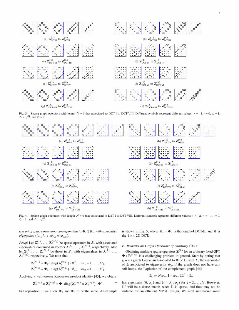
The rectangular patterns we observe in (17) can be simply extended toany arbitrary transform length N (e.g., all such operators with N = 6are shown in Fig. 3(b)). We also show the associated eigenvalues ofZ(`)DCT-II with arbitrary N in Table I. Note that all the operators and

their associated graphs are sparse. In particular, each operator has atmost 2N non-zero entries and its corresponding graph has at mostN − 1 edges.

5

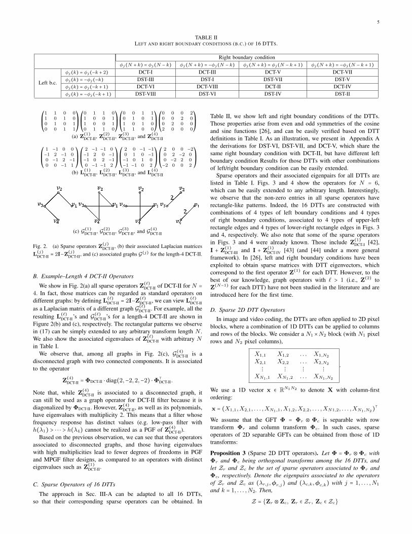
TABLE IILEFT AND RIGHT BOUNDARY CONDITIONS (B.C.) OF 16 DTTS.

Right boundary conditionφj(N + k) = φj(N − k) φj(N + k) = −φj(N − k) φj(N + k) = φj(N − k + 1) φj(N + k) = −φj(N − k + 1)

Left b.c.

φj(k) = φj(−k + 2) DCT-I DCT-III DCT-V DCT-VIIφj(k) = −φj(−k) DST-III DST-I DST-VII DST-Vφj(k) = φj(−k + 1) DCT-VI DCT-VIII DCT-II DCT-IVφj(k) = −φj(−k + 1) DST-VIII DST-VI DST-IV DST-II

⎛⎜⎝

1 1 0 01 0 1 00 1 0 10 0 1 1

⎞⎟⎠

⎛⎜⎝

0 1 1 01 0 0 11 0 0 10 1 1 0

⎞⎟⎠

⎛⎜⎝

0 0 1 10 1 0 11 0 1 01 1 0 0

⎞⎟⎠

⎛⎜⎝

0 0 0 20 0 2 00 2 0 02 0 0 0

⎞⎟⎠

(a) Z(1)DCT-II, Z

(2)DCT-II, Z

(3)DCT-II, and Z

(4)DCT-II

⎛⎜⎝

1 −1 0 0−1 2 −1 00 −1 2 −10 0 −1 1

⎞⎟⎠

⎛⎜⎝

2 −1 −1 0−1 2 0 −1−1 0 2 −10 −1 −1 2

⎞⎟⎠

⎛⎜⎝

2 0 −1 −10 1 0 −1−1 0 1 0−1 −1 0 2

⎞⎟⎠

⎛⎜⎝

2 0 0 −20 2 −2 00 −2 2 0−2 0 0 2

⎞⎟⎠

(b) L(1)DCT-II, L

(2)DCT-II, L

(3)DCT-II, and L

(4)DCT-II

(c) G(1)DCT-II, G(2)DCT-II, G

(3)DCT-II, and G(4)DCT-II

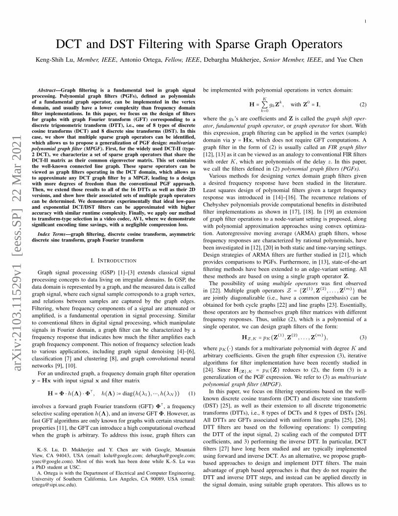
Fig. 2. (a) Sparse operators Z(j)DCT-II, (b) their associated Laplacian matrices

L(j)DCT-II = 2I−Z

(j)DCT-II, and (c) associated graphs G(j) for the length-4 DCT-II.

B. Example–Length 4 DCT-II Operators

We show in Fig. 2(a) all sparse operators Z(`)DCT-II of DCT-II for N =

4. In fact, those matrices can be regarded as standard operators ondifferent graphs: by defining L

(`)DCT-II = 2I−Z

(`)DCT-II, we can view L

(`)DCT-II

as a Laplacian matrix of a different graph G(`)DCT-II. For example, all theresulting L

(`)DCT-II’s and G(`)DCT-II’s for a length-4 DCT-II are shown in

Figure 2(b) and (c), respectively. The rectangular patterns we observein (17) can be simply extended to any arbitrary transform length N .We also show the associated eigenvalues of Z

(`)DCT-II with arbitrary N

in Table I.We observe that, among all graphs in Fig. 2(c), G(4)DCT-II is a

disconnected graph with two connected components. It is associatedto the operator

Z(4)DCT-II = ΦDCT-II ⋅ diag(2,−2,2,−2) ⋅Φ⊺

DCT-II.

Note that, while Z(4)DCT-II is associated to a disconnected graph, it

can still be used as a graph operator for DCT-II filter because it isdiagonalized by ΦDCT-II. However, Z

(4)DCT-II, as well as its polynomials,

have eigenvalues with multiplicity 2. This means that a filter whosefrequency response has distinct values (e.g. low-pass filter withh(λ1) > ⋅ ⋅ ⋅ > h(λ4) cannot be realized as a PGF of Z

(4)DCT-II).

Based on the previous observation, we can see that those operatorsassociated to disconnected graphs, and those having eigenvalueswith high multiplicities lead to fewer degrees of freedoms in PGFand MPGF filter designs, as compared to an operators with distincteigenvalues such as Z

(1)DCT-II.

C. Sparse Operators of 16 DTTs

The approach in Sec. III-A can be adapted to all 16 DTTs,so that their corresponding sparse operators can be obtained. In

Table II, we show left and right boundary conditions of the DTTs.Those properties arise from even and odd symmetries of the cosineand sine functions [26], and can be easily verified based on DTTdefinitions in Table I. As an illustration, we present in Appendix Athe derivations for DST-VI, DST-VII, and DCT-V, which share thesame right boundary condition with DCT-II, but have different leftboundary condition Results for those DTTs with other combinationsof left/right boundary condition can be easily extended.

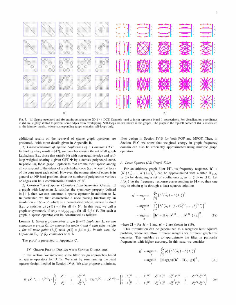
Sparse operators and their associated eigenpairs for all DTTs arelisted in Table I. Figs. 3 and 4 show the operators for N = 6,which can be easily extended to any arbitrary length. Interestingly,we observe that the non-zero entries in all sparse operators haverectangle-like patterns. Indeed, the 16 DTTs are constructed withcombinations of 4 types of left boundary conditions and 4 typesof right boundary conditions, associated to 4 types of upper-leftrectangle edges and 4 types of lower-right rectangle edges in Figs. 3and 4, respectively. We also note that some of the sparse operatorsin Figs. 3 and 4 were already known. Those include Z

(1)DCT-I [42],

I + Z(1)DCT-III and I + Z

(1)DCT-IV [43] (and [44] under a more general

framework). In [26], left and right boundary conditions have beenexploited to obtain sparse matrices with DTT eigenvectors, whichcorrespond to the first operator Z(1) for each DTT. However, to thebest of our knowledge, graph operators with ` > 1 (i.e., Z(2) toZ(N−1) for each DTT) have not been studied in the literature and areintroduced here for the first time.

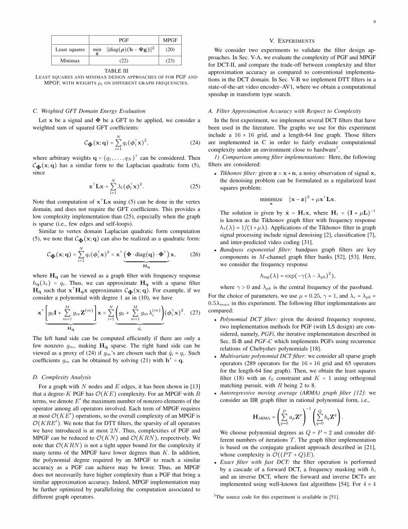
D. Sparse 2D DTT Operators

In image and video coding, the DTTs are often applied to 2D pixelblocks, where a combination of 1D DTTs can be applied to columnsand rows of the blocks. We consider a N1×N2 block (with N1 pixelrows and N2 pixel columns),

X1,1 X1,2 . . . X1,N2

X2,1 X2,2 . . . X2,N2

⋮ ⋮ ⋮ ⋮

XN1,1 XN1,2 . . . XN1,N2

.

We use a 1D vector x ∈ RN1N2 to denote X with column-firstordering:

x = (X1,1,X2,1, . . . ,XN1,1,X1,2,X2,2, . . . ,XN1,2, . . . ,XN1,N2)⊺

We assume that the GFT Φ = Φr ⊗ Φc is separable with rowtransform Φr and column transform Φc. In such cases, sparseoperators of 2D separable GFTs can be obtained from those of 1Dtransforms:

Proposition 3 (Sparse 2D DTT operators). Let Φ = Φr ⊗Φc withΦr and Φc being orthogonal transforms among the 16 DTTs, andlet Zr and Zc be the set of sparse operators associated to Φr andΦc, respectively. Denote the eigenpairs associated to the operatorsof Zr and Zc as (λr,j ,φr,j) and (λc,k,φc,k) with j = 1, . . . ,N1

and k = 1, . . . ,N2. Then,

Z = {Zr ⊗Zc, Zr ∈ Zr, Zc ∈ Zc}

6

(a) Z(1)DCT-I to Z

(5)DCT-I (b) Z

(1)DCT-II to Z

(6)DCT-II

(c) Z(1)DCT-III to Z

(5)DCT-III (d) Z

(1)DCT-IV to Z

(5)DCT-IV

(e) Z(1)DCT-V to Z

(5)DCT-V (f) Z

(1)DCT-VI to Z

(5)DCT-VI

(g) Z(1)DCT-VII to Z

(5)DCT-VII (h) Z

(1)DCT-VIII to Z

(6)DCT-VIII

Fig. 3. Sparse graph operators with length N = 6 that associated to DCT-I to DCT-VIII. Different symbols represent different values: × = −1, ⋅ = 0, ◯ = 1,△ =√2, and ◻ = 2.

(a) Z(1)DST-I to Z

(7)DST-I (b) Z

(1)DST-II to Z

(6)DST-II

(c) Z(1)DST-III to Z

(5)DST-III (d) Z

(1)DST-IV to Z

(5)DST-IV

(e) Z(1)DST-V to Z

(6)DST-V (f) Z

(1)DST-VI to Z

(6)DST-VI

(g) Z(1)DST-VII to Z

(6)DST-VII (h) Z

(1)DST-VIII to Z

(5)DST-VIII

Fig. 4. Sparse graph operators with length N = 6 that associated to DST-I to DST-VIII. Different symbols represent different values: + = −2, × = −1, ⋅ = 0,◯ = 1, and △ =

√2.

is a set of sparse operators corresponding to Φr⊗Φc, with associatedeigenpairs (λr,jλc,k,φr,j ⊗φc,k).

Proof: Let Z(1)r , . . . , Z

(M1)r be sparse operators in Zr with associated

eigenvalues contained in vectors λ(1)r , . . . , λ(M1)r , respectively. Also

let Z(1)c , . . . , Z

(M1)c be those in Zc with eigenvalues in λ(1)c , . . . ,

λ(M2)c , respectively. We note that

Z(m1)r = Φr ⋅ diag(λ(m1)

r ) ⋅Φ⊺r , m1 = 1, . . . ,M1,

Z(m2)c = Φc ⋅ diag(λ(m2)

c ) ⋅Φ⊺c , m2 = 1, . . . ,M2.

Applying a well-known Kronecker product identity [45], we obtain

Z(m1)r ⊗Z(m2)

c = Φ ⋅ diag(λ(m1)r ⊗λ(m2)

c ) ⋅Φ⊺.

In Proposition 3, we allow Φc and Φr to be the same. An example

is shown in Fig. 5, where Φc = Φr is the length-4 DCT-II, and Φ isthe 4 × 4 2D DCT.

E. Remarks on Graph Operators of Arbitrary GFTs

Obtaining multiple sparse operators Z(k) for an arbitrary fixed GFTΦ ∈ RN×N is a challenging problem in general. Start by noting thatgiven a graph Laplacian associated to Φ be L, with λj the eigenvalueof L associated to eigenvector φj , if the graph does not have anyself-loops, the Laplacian of the complement graph [46]

Lc ∶= NwmaxI −wmax11⊺ −L,

has eigenpairs (0,φ1) and (n − λj ,φj) for j = 2, . . . ,N . However,Lc will be a dense matrix when L is sparse, and thus may not besuitable for an efficient MPGF design. We next summarize some

7

(a) (b)

Fig. 5. (a) Sparse operators and (b) graphs associated to 2D 4×4 DCT. Symbols ⋅ and ◯ in (a) represent 0 and 1, respectively. For visualization, coordinatesin (b) are slightly shifted to prevent some edges from overlapping. Self-loops are not shown in the graphs. The graph in the top-left corner of (b) is associatedto the identity matrix, whose corresponding graph contains self-loops only.

additional results on the retrieval of sparse graph operators arepresented, with more details given in Appendix B.

1) Characterization of Sparse Laplacians of a Common GFT:Extending a key result in [47], we can characterize the set of all graphLaplacians (i.e., those that satisfy (4) with non-negative edge and self-loop weights) sharing a given GFT Φ by a convex polyhedral cone.In particular, those graph Laplacians that are the most sparse amongall correspond to the edges of a polyhedral cone (i.e., where the facesof the cone meet each other). However, the enumeration of edges is ingeneral an NP-hard problem since the number of polyhedron verticesor edges can be a combinatorial number of N .

2) Construction of Sparse Operators from Symmetric Graphs: Ifa graph with Laplacian L satisfies the symmetry property definedin [11], then we can construct a sparse operator in addition to L.In particular, we first characterize a node pairing function by aninvolution ϕ ∶ V → V , which is a permutation whose inverse is itself(i.e., ϕ satisfies ϕ(ϕ(i)) = i for all i ∈ V). In this way, we call agraph ϕ-symmetric if wi,j = wϕ(i),ϕ(j) for all i, j ∈ V . For such agraph, a sparse operator can be constructed as follows:

Lemma 1. Given a ϕ-symmetric graph G with Laplacian L, we canconstruct a graph Gϕ by connecting nodes i and j with edge weight1 for all node pairs (i, j) with ϕ(i) = j, i ≠ j). In this way, theLaplacian Lϕ of Gϕ commutes with L.

The proof is presented in Appendix C.

IV. GRAPH FILTER DESIGN WITH SPARSE OPERATORS

In this section, we introduce some filter design approaches basedon sparse operators for DTTs. We start by summarizing the leastsquares design method in Section IV-A. We also propose a minimax

filter design in Section IV-B for both PGF and MPGF. Then, inSection IV-C we show that weighted energy in graph frequencydomain can also be efficiently approximated using multiple graphoperators.

A. Least Squares (LS) Graph Filter

For an arbitrary graph filter H∗, its frequency response, h∗ =

(h∗(λ1), . . . , h∗(λN))

⊺, can be approximated with a filter HZ,Kin (3) by designing a set of coefficients g as in (10) or (11). Leth(λj) be the frequency response corresponding to HZ,K , then oneway to obtain g is through a least squares solution:

g∗ = argming

N

∑j=1

(h∗(λj) − h(λj))2

= argming

N

∑j=1

(h∗(λj) − pK(λ(1)j , . . . , λ

(M)j ))

2

= argming

∥h∗ −ΠK(λ(1), . . . ,λ(M)) ⋅ g∥2, (18)

where ΠK for K = 1 and K = 2 are shown in (19).This formulation can be generalized to a weighted least squares

problem, where we allow different weights for different graph fre-quencies. This enables us to approximate the filter in particularfrequencies with higher accuracy. In this case, we consider

g∗ = argming

N

∑j=1

ρ2i (h∗(λj) − h(λj))

2

= argming

∥diag(ρ)(h∗ −ΠK ⋅ g)∥2, (20)

Π1(λ(1), . . . ,λ

(M)) =

⎛

⎜⎜

⎝

1 λ(1)1 . . . λ

(M)

1⋮ ⋮ ⋮ ⋮

1 λ(1)N

. . . λ(M)

N

⎞

⎟⎟

⎠

, Π2(λ(1), . . . ,λ

(M)) =

⎛

⎜⎜

⎝

1 λ(1)1 . . . λ

(M)

1 λ(1)1 λ

(1)1 λ

(1)1 λ

(2)1 . . . λ

(M)

1 λ(M)

1⋮ ⋮ ⋮ ⋮ ⋮ ⋮ ⋮

1 λ(1)N

. . . λ(M)

Nλ(1)Nλ(1)N

λ(1)Nλ(2)N

. . . λ(M)

Nλ(M)

N

⎞

⎟⎟

⎠

. (19)

8

0 1 2 3 4

Graph frequency

-0.2

0

0.2

0.4

0.6

0.8

1F

req

ue

ncy r

esp

on

se

Desired

PGF, K=2

PGF, K=3

MPGF, p1(Z

(4),Z

(7))

MPGF, p1(Z

(4),Z

(7),Z

(10))

Fig. 6. An example for PGF and MPGF fitting results on a length 12 linegraph. The desired frequency response is h∗(λ) = exp(−4(λ − 1)2). ThePGF and MPGF filters have been optimized based on (2) and (18).

where ρi ≥ 0 is the weight corresponding to λi. Note that whenρ = 1, the problem (20) reduces to (18).

When g is sparser, (i.e., its `0 norm is smaller), fewer terms willbe involved in the polynomial pK , leading to a lower complexity forthe filtering operation. This `0-constrained problem can be viewedas a sparse representation of diag(ρ)h∗ in an overcomplete dic-tionary diag(ρ)ΠK . Well-known methods for this problem includethe orthogonal matching pursuit (OMP) algorithm [48], and theoptimization with a sparsity-promoting `1 constraint:

minimizeg

∥diag(ρ)(h∗ −ΠK ⋅ g)∥2

subject to ∥g∥1 ≤ τ,

(21)where τ is a pre-chosen threshold. In fact, this formulation can beviewed as an extension of its PGF counterpart [18] to an MPGFsetting. Note that (21) is a `1-constrained least squares problem(a.k.a., the LASSO problem), where efficient solvers are available[49].

Compared to conventional PGF H in (2), the implementationwith HZ,K has several advantages. First, when K = 1, the MPGF(10) is a linear combination of different sparse operators, which isamenable to parallelization. This is in contrast to high degree PGFsbased on (2), which require applying the graph operator repeatedly.Second, HZ,K is a generalization of H and provides more degreesof freedom, which provides more accurate approximation with equalor lower order polynomial. Note that, while the eigenvalues of Zk fork = 1,2, . . . are typically all increasing (if Z = L) or decreasing (if,for instance, Z = 2I−L), those of different Z(m)’s have more diversedistributions (i.e., increasing, decreasing, or non-monotonic). Thus,MPGFs provide better approximations for filters with non-monotonicfrequency responses. For example, we demonstrate in Fig. 6 theresulting PGF and MPGF for a bandpass filter. We can see that,for K = 2 and K = 3, a degree-1 MPGF with K operators givesa higher approximation accuracy than a degree-K PGF, while theyhave a similar complexity.

B. Minimax Graph Filter

The minimax approach is a popular filter design method in classicalsignal processing. The goal is to design an length-K FIR filter whosefrequency response G(ejω) approximates the desired frequency re-sponse H(ejω) in a way that the maximum error within some rangeof frequency is minimized. A standard design method is the Parks-McClellan algorithm, which is a variation of the Remez exchangealgorithm [50].

0 1 2 3 4

Graph frequency

0

0.5

1

1.5

Fre

qu

en

cy r

esp

on

se

passband transitionband

stopbandDesired

LS, unweighted

LS, weighted

Minimax, unweighted

Minimax, weighted

Fig. 7. Example illustrating the frequency responses of degree K = 4 PGFwith least squares (LS) and minimax criteria, with weighted or unweightedsettings. The filters are defined on a length 24 line graph. In the weightedsetting, weights ρi are chosen to be 2, 0, and 1 for passband, transition band,and stopband, respectively.

Here, we explore minimax design criteria for graph filters. Wedenote h∗(λ) the desired frequency response, and g(λ) the polyno-mial filter that approximates h∗(λ). Source code for the proposedminimax graph filter design methods can be found in [51].

1) Polynomial Graph Filter: Let g(λ) be the PGF with degreeK given by (2). Since graph frequencies λ1, . . . , λN are discrete,we only need to minimize the maximum error between h∗ and gat frequencies λ1, . . . , λN . In particular, we would like to solvepolynomial coefficients gi:

minimizeb

maxiρi

RRRRRRRRRRR

h∗(λi) −K

∑j=0

gjλji

RRRRRRRRRRR´¹¹¹¹¹¹¹¹¹¹¹¹¹¹¹¹¹¹¹¹¹¹¹¹¹¹¹¹¹¹¹¹¹¹¹¹¹¹¹¹¹¹¹¹¹¹¹¹¹¹¹¹¹¹¹¹¹¹¹¹¹¹¹¹¹¹¹¹¹¹¹¹¹¹¹¹¹¹¸¹¹¹¹¹¹¹¹¹¹¹¹¹¹¹¹¹¹¹¹¹¹¹¹¹¹¹¹¹¹¹¹¹¹¹¹¹¹¹¹¹¹¹¹¹¹¹¹¹¹¹¹¹¹¹¹¹¹¹¹¹¹¹¹¹¹¹¹¹¹¹¹¹¹¹¹¹¶

∥diag(ρ)(h∗−Ψg)∥∞

where Ψ is the matrix in (6), ρi is the weight associated to λi and∥⋅∥∞ represents the infinity norm. Note that, when K ≥ N−1 and Ψ isfull row rank, then h∗ = Ψg can be achieved with g = Ψ†h∗. Other-wise, we reduce this problem by setting ε = ∥diag(ρ) (h∗ −Ψg) ∥∞:

minimizeg, ε

ε subject to − ε1 ⪯ diag(ρ) (h∗ −Ψg) ⪯ ε1, (22)

whose solution can be efficiently obtained with a linear programmingsolver.

2) Multivariate Polynomial Graph Filter: Now we consider g(λ)a graph filter with M graph operators with degree K, as in (3). Inthis case, we can simply extend the problem (22) to

minimizeg, ε

ε subject to − ε1 ⪯ diag(ρ) (h∗ −ΠKg) ⪯ ε1, (23)

where a `1 or `0 norm constraint on g can also be considered.To summarize, we show in Table III the objective functions of least

squares and minimax designs with PGF and MPGF, where weightson different graph frequencies are considered. Note that the leastsquares PGF design shown in Table III is a simple extension of theunweighted design (6) in [15].

Using an ideal low-pass filter as the desired filter, we show a toyexample with degree-4 PGF in Fig. 7. When different weights ρiare used for passband, transition band, and stopband, approximationaccuracies differ for different graph frequencies. By comparing LSand minimax results in a weighted setting, we also see that the min-imax criterion yields a smaller maximum error within the passband(see the last frequency bin in passband) and stopband (see the firstfrequency bin in stopband).

9

PGF MPGF

Least squares ming

∣∣diag(ρ)(h −Ψg)∣∣2 (20)

Minimax (22) (23)

TABLE IIILEAST SQUARES AND MINIMAX DESIGN APPROACHES OF FOR PGF AND

MPGF, WITH WEIGHTS ρi ON DIFFERENT GRAPH FREQUENCIES.

C. Weighted GFT Domain Energy Evaluation

Let x be a signal and Φ be a GFT to be applied, we consider aweighted sum of squared GFT coefficients:

CΦ(x;q) =N

∑i=1qi(φ

⊺i x)

2, (24)

where arbitrary weights q = (q1, . . . , qN)⊺ can be considered. Then

CΦ(x;q) has a similar form to the Laplacian quadratic form (5),since

x⊺Lx =N

∑l=1λl(φ

⊺l x)

2. (25)

Note that computation of x⊺Lx using (5) can be done in the vertexdomain, and does not require the GFT coefficients. This provides alow complexity implementation than (25), especially when the graphis sparse (i.e., few edges and self-loops).

Similar to vertex domain Laplacian quadratic form computation(5), we note that CΦ(x;q) can also be realized as a quadratic form:

CΦ(x;q) =N

∑i=1qi(φ

⊺i x)

2= x⊺ (Φ ⋅ diag(q) ⋅Φ⊺

)

´¹¹¹¹¹¹¹¹¹¹¹¹¹¹¹¹¹¹¹¹¹¹¹¹¹¹¹¹¹¹¹¹¹¹¹¹¹¹¹¹¹¹¹¹¹¹¹¹¹¸¹¹¹¹¹¹¹¹¹¹¹¹¹¹¹¹¹¹¹¹¹¹¹¹¹¹¹¹¹¹¹¹¹¹¹¹¹¹¹¹¹¹¹¹¹¹¹¹¹¶Hq

x, (26)

where Hq can be viewed as a graph filter with frequency responsehq(λi) = qi. Thus, we can approximate Hq with a sparse filterHq such that x⊺Hqx approximates CΦ(x;q). For example, if weconsider a polynomial with degree 1 as in (10), we have

x⊺ [g0I +M

∑m=1

gmZ(m)]

´¹¹¹¹¹¹¹¹¹¹¹¹¹¹¹¹¹¹¹¹¹¹¹¹¹¹¹¹¹¹¹¹¹¹¹¹¹¹¹¹¹¹¹¹¹¹¹¹¹¹¹¹¹¹¹¹¹¸¹¹¹¹¹¹¹¹¹¹¹¹¹¹¹¹¹¹¹¹¹¹¹¹¹¹¹¹¹¹¹¹¹¹¹¹¹¹¹¹¹¹¹¹¹¹¹¹¹¹¹¹¹¹¹¹¹¶Hq

x =N

∑i=1

(g0 +M

∑m=1

gmλ(m)i )

´¹¹¹¹¹¹¹¹¹¹¹¹¹¹¹¹¹¹¹¹¹¹¹¹¹¹¹¹¹¹¹¹¹¹¹¹¹¹¹¹¹¹¹¹¹¹¹¹¹¹¹¹¹¸¹¹¹¹¹¹¹¹¹¹¹¹¹¹¹¹¹¹¹¹¹¹¹¹¹¹¹¹¹¹¹¹¹¹¹¹¹¹¹¹¹¹¹¹¹¹¹¹¹¹¹¹¹¶qi

(φ⊺i x)2. (27)

The left hand side can be computed efficiently if there are only afew nonzero gm, making Hq sparse. The right hand side can beviewed as a proxy of (24) if gm’s are chosen such that qi ≈ qi. Suchcoefficients gm can be obtained by solving (21) with h∗ = q.

D. Complexity Analysis

For a graph with N nodes and E edges, it has been shown in [13]that a degree-K PGF has O(KE) complexity. For an MPGF with Rterms, we denote E′ the maximum number of nonzero elements of theoperator among all operators involved. Each term of MPGF requiresat mostO(KE′

) operations, so the overall complexity of an MPGF isO(KRE′

). We note that for DTT filters, the sparsity of all operatorswe have introduced is at most 2N . Thus, complexities of PGF andMPGF can be reduced to O(KN) and O(KRN), respectively. Wenote that O(KRN) is not a tight upper bound for the complexity ifmany terms of the MPGF have lower degrees than K. In addition,the polynomial degree required by an MPGF to reach a similaraccuracy as a PGF can achieve may be lower. Thus, an MPGFdoes not necessarily have higher complexity than a PGF that bring asimilar approximation accuracy. Indeed, MPGF implementation maybe further optimized by parallelizing the computation associated todifferent graph operators.

V. EXPERIMENTS

We consider two experiments to validate the filter design ap-proaches. In Sec. V-A, we evaluate the complexity of PGF and MPGFfor DCT-II, and compare the trade-off between complexity and filterapproximation accuracy as compared to conventional implementa-tions in the DCT domain. In Sec. V-B we implement DTT filters in astate-of-the-art video encoder–AV1, where we obtain a computationalspeedup in transform type search.

A. Filter Approximation Accuracy with Respect to Complexity

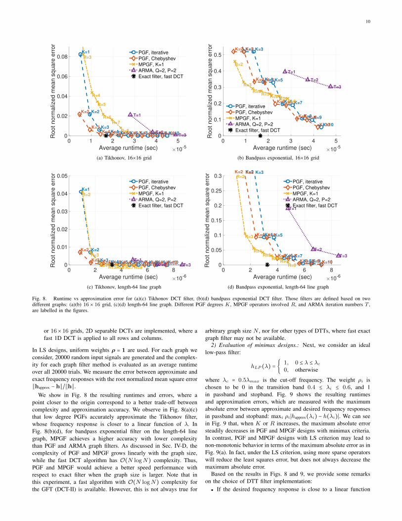
In the first experiment, we implement several DCT filters that havebeen used in the literature. The graphs we use for this experimentinclude a 16 × 16 grid, and a length-64 line graph. Those filtersare implemented in C in order to fairly evaluate computationalcomplexity under an environment close to hardware3.

1) Comparison among filter implementations: Here, the followingfilters are considered:

● Tikhonov filter: given z = x+n, a noisy observation of signal x,the denoising problem can be formulated as a regularized leastsquares problem:

minimizex

∥x − z∥2 + µx⊺Lx.

The solution is given by x = Htx, where Ht = (I + µL)−1

is known as the Tikhonov graph filter with frequency responseht(λ) = 1/(1+µλ). Applications of the Tikhonov filter in graphsignal processing include signal denoising [2], classification [7],and inter-predicted video coding [31].

● Bandpass exponential filter: bandpass graph filters are keycomponents in M -channel graph filter banks [52], [53]. Here,we consider the frequency response

hexp(λ) = exp(−γ(λ − λpb)2),

where γ > 0 and λpb is the central frequency of the passband.For the choice of parameters, we use µ = 0.25, γ = 1, and λc = λpb =0.5λmax in this experiment. The following filter implementations arecompared:

● Polynomial DCT filter: given the desired frequency response,two implementation methods for PGF (with LS design) are con-sidered, namely, PGFi, the iterative implementation described inSec. II-B and PGF-C which implements PGFs using recurrencerelations of Chebyshev polynomials [18].

● Multivariate polynomial DCT filter: we consider all sparse graphoperators (289 operators for the 16 × 16 grid and 65 operatorsfor the length-64 line graph). Then, we obtain the least squaresfilter (18) with an `0 constraint and K = 1 using orthogonalmatching pursuit, with R being 2 to 8.

● Autoregressive moving average (ARMA) graph filter [12]: weconsider an IIR graph filter in rational polynomial form, i.e.,

HARMA =⎛

⎝

P

∑p=0

apZp⎞

⎠

−1⎛

⎝

Q

∑q=0

bqZq⎞

⎠.

We choose polynomial degrees as Q = P = 2 and consider dif-ferent numbers of iterations T . The graph filter implementationis based on the conjugate gradient approach described in [21],whose complexity is O((PT +Q)E).

● Exact filter with fast DCT: the filter operation is performedby a cascade of a forward DCT, a frequency masking with h,and an inverse DCT, where the forward and inverse DCTs areimplemented using well-known fast algorithms [54]. For 4 × 4

3The source code for this experiment is available in [51].

10

0 1 2 3 4 5

Average runtime (sec) 10-5

0

0.02

0.04

0.06

0.08R

oot norm

aliz

ed m

ean s

quare

err

or

K=1

K=2

K=3

K=4 K=5 K=6 K=7 K=8 K=9 K=10

K=2

K=3

K=4 K=5 K=6 K=7 K=8 K=9 K=10

R=3

R=4

R=5

R=6

R=7

R=8

T=1

T=2T=3

PGF, iterative

PGF, Chebyshev

MPGF, K=1

ARMA, Q=2, P=2

Exact filter, fast DCT

(a) Tikhonov, 16×16 grid

0 1 2 3 4 5

Average runtime (sec) 10-5

0

0.1

0.2

0.3

0.4

0.5

Root norm

aliz

ed m

ean s

quare

err

or

K=2 K=3

K=4 K=5

K=6 K=7

K=8 K=9

K=10

K=2 K=3

K=4 K=5

K=6 K=7

K=8 K=9

K=10

R=2

R=3

R=4R=5

R=6R=7

R=8

T=1

T=2

T=3

PGF, iterative

PGF, Chebyshev

MPGF, K=1

ARMA, Q=2, P=2

Exact filter, fast DCT

(b) Bandpass exponential, 16×16 grid

0 2 4 6 8

Average runtime (sec) 10-6

0

0.01

0.02

0.03

0.04

0.05

Root norm

aliz

ed m

ean s

quare

err

or

K=1

K=2

K=3K=4 K=5 K=6 K=7 K=8K=9 K=10

K=2

K=3K=4 K=5 K=6 K=7 K=8 K=9 K=10

R=2

R=3

R=4R=5R=6 R=7 R=8

T=1

T=2 T=3

PGF, iterative

PGF, Chebyshev

MPGF, K=1

ARMA, Q=2, P=2

Exact filter, fast DCT

(c) Tikhonov, length-64 line graph

0 2 4 6 8

Average runtime (sec) 10-6

0

0.05

0.1

0.15

0.2

0.25

0.3

Root norm

aliz

ed m

ean s

quare

err

or K=2 K=3

K=4 K=5

K=6 K=7

K=8 K=9 K=10

K=2 K=3

K=4 K=5

K=6 K=7

K=8 K=9 K=10

R=2

R=3

R=4

R=5R=6

R=7R=8

T=1

T=2

T=3

PGF, iterative

PGF, Chebyshev

MPGF, K=1

ARMA, Q=2, P=2

Exact filter, fast DCT

(d) Bandpass exponential, length-64 line graph

Fig. 8. Runtime vs approximation error for (a)(c) Tikhonov DCT filter, (b)(d) bandpass exponential DCT filter. Those filters are defined based on twodifferent graphs: (a)(b) 16 × 16 grid, (c)(d) length-64 line graph. Different PGF degrees K, MPGF operators involved R, and ARMA iteration numbers T ,are labelled in the figures.

or 16× 16 grids, 2D separable DCTs are implemented, where afast 1D DCT is applied to all rows and columns.

In LS designs, uniform weights ρ = 1 are used. For each graph weconsider, 20000 random input signals are generated and the complex-ity for each graph filter method is evaluated as an average runtimeover all 20000 trials. We measure the error between approximate andexact frequency responses with the root normalized mean square error∥happrox − h∥/∥h∥.

We show in Fig. 8 the resulting runtimes and errors, where apoint closer to the origin correspond to a better trade-off betweencomplexity and approximation accuracy. We observe in Fig. 8(a)(c)that low degree PGFs accurately approximate the Tikhonov filter,whose frequency response is closer to a linear function of λ. InFig. 8(b)(d), for bandpass exponential filter on the length-64 linegraph, MPGF achieves a higher accuracy with lower complexitythan PGF and ARMA graph filters. As discussed in Sec. IV-D, thecomplexity of PGF and MPGF grows linearly with the graph size,while the fast DCT algorithm has O(N logN) complexity. Thus,PGF and MPGF would achieve a better speed performance withrespect to exact filter when the graph size is larger. Note that inthis experiment, a fast algorithm with O(N logN) complexity forthe GFT (DCT-II) is available. However, this is not always true for

arbitrary graph size N , nor for other types of DTTs, where fast exactgraph filter may not be available.

2) Evaluation of minimax designs.: Next, we consider an ideallow-pass filter:

hLP (λ) = {1, 0 ≤ λ ≤ λc0, otherwise

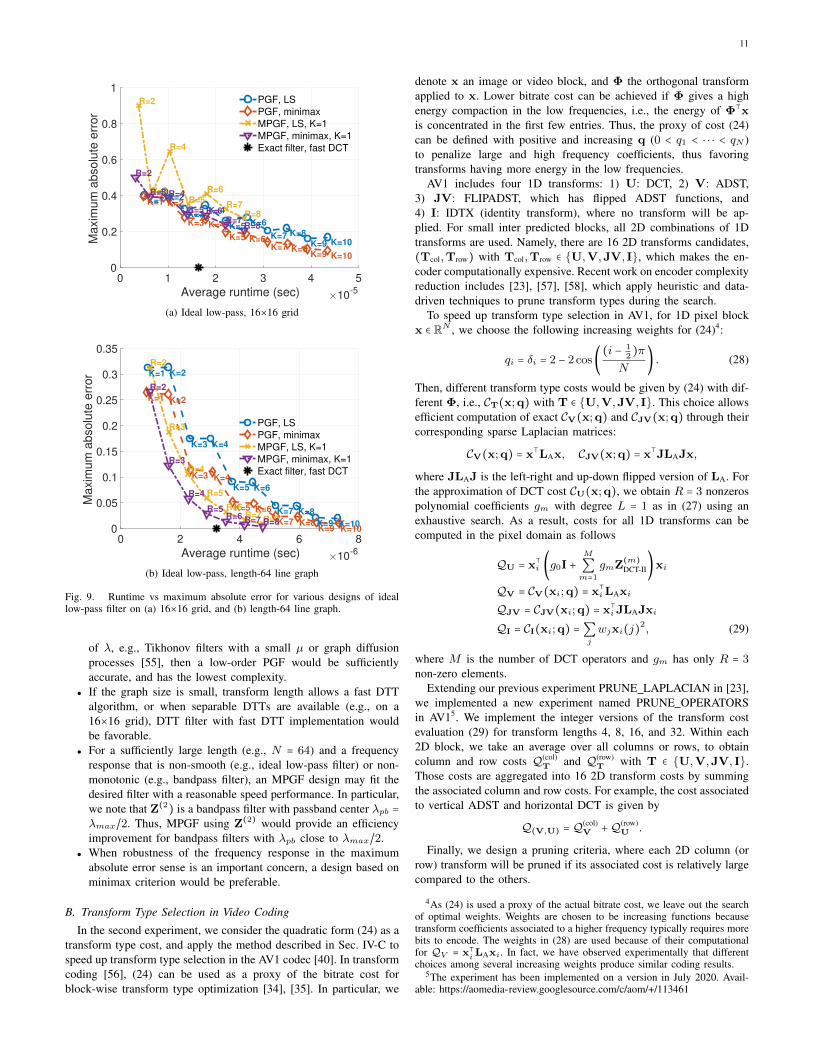
where λc = 0.5λmax is the cut-off frequency. The weight ρi ischosen to be 0 in the transition band 0.4 ≤ λi ≤ 0.6, and 1in passband and stopband. Fig. 9 shows the resulting runtimesand approximation errors, which are measured with the maximumabsolute error between approximate and desired frequency responsesin passband and stopband: maxi ρi∣happrox(λi) − h(λi)∣. We can seein Fig. 9 that, when K or R increases, the maximum absolute errorsteadily decreases in PGF and MPGF designs with minimax criteria.In contrast, PGF and MPGF designs with LS criterion may lead tonon-monotonic behavior in terms of the maximum absolute error as inFig. 9(a). In fact, under the LS criterion, using more sparse operatorswill reduce the least squares error, but does not always decrease themaximum absolute error.

Based on the results in Figs. 8 and 9, we provide some remarkson the choice of DTT filter implementation:

● If the desired frequency response is close to a linear function

11

0 1 2 3 4 5

Average runtime (sec) 10-5

0

0.2

0.4

0.6

0.8

1M

axim

um

absolu

te e

rror

K=1K=2

K=3K=4

K=5K=6

K=7 K=8

K=9 K=10

K=1 K=2

K=3 K=4

K=5 K=6K=7 K=8

K=9 K=10

R=2

R=3

R=4

R=5

R=6

R=7

R=8

R=2

R=3 R=4

R=5 R=6

R=7R=8

PGF, LS

PGF, minimax

MPGF, LS, K=1

MPGF, minimax, K=1

Exact filter, fast DCT

(a) Ideal low-pass, 16×16 grid

0 2 4 6 8

Average runtime (sec) 10-6

0

0.05

0.1

0.15

0.2

0.25

0.3

0.35

Maxim

um

absolu

te e

rror K=1 K=2

K=3 K=4

K=5 K=6

K=7 K=8

K=9 K=10

K=1 K=2

K=3 K=4

K=5 K=6

K=7 K=8K=9 K=10

R=2

R=3

R=4

R=5

R=6R=7

R=8

R=2

R=3

R=4

R=5R=6

R=7 R=8

PGF, LS

PGF, minimax

MPGF, LS, K=1

MPGF, minimax, K=1

Exact filter, fast DCT

(b) Ideal low-pass, length-64 line graph

Fig. 9. Runtime vs maximum absolute error for various designs of ideallow-pass filter on (a) 16×16 grid, and (b) length-64 line graph.

of λ, e.g., Tikhonov filters with a small µ or graph diffusionprocesses [55], then a low-order PGF would be sufficientlyaccurate, and has the lowest complexity.

● If the graph size is small, transform length allows a fast DTTalgorithm, or when separable DTTs are available (e.g., on a16×16 grid), DTT filter with fast DTT implementation wouldbe favorable.

● For a sufficiently large length (e.g., N = 64) and a frequencyresponse that is non-smooth (e.g., ideal low-pass filter) or non-monotonic (e.g., bandpass filter), an MPGF design may fit thedesired filter with a reasonable speed performance. In particular,we note that Z(2) is a bandpass filter with passband center λpb =λmax/2. Thus, MPGF using Z(2) would provide an efficiencyimprovement for bandpass filters with λpb close to λmax/2.

● When robustness of the frequency response in the maximumabsolute error sense is an important concern, a design based onminimax criterion would be preferable.

B. Transform Type Selection in Video Coding

In the second experiment, we consider the quadratic form (24) as atransform type cost, and apply the method described in Sec. IV-C tospeed up transform type selection in the AV1 codec [40]. In transformcoding [56], (24) can be used as a proxy of the bitrate cost forblock-wise transform type optimization [34], [35]. In particular, we

denote x an image or video block, and Φ the orthogonal transformapplied to x. Lower bitrate cost can be achieved if Φ gives a highenergy compaction in the low frequencies, i.e., the energy of Φ⊺xis concentrated in the first few entries. Thus, the proxy of cost (24)can be defined with positive and increasing q (0 < q1 < ⋅ ⋅ ⋅ < qN )to penalize large and high frequency coefficients, thus favoringtransforms having more energy in the low frequencies.

AV1 includes four 1D transforms: 1) U: DCT, 2) V: ADST,3) JV: FLIPADST, which has flipped ADST functions, and4) I: IDTX (identity transform), where no transform will be ap-plied. For small inter predicted blocks, all 2D combinations of 1Dtransforms are used. Namely, there are 16 2D transforms candidates,(Tcol,Trow) with Tcol,Trow ∈ {U,V,JV, I}, which makes the en-coder computationally expensive. Recent work on encoder complexityreduction includes [23], [57], [58], which apply heuristic and data-driven techniques to prune transform types during the search.

To speed up transform type selection in AV1, for 1D pixel blockx ∈ RN , we choose the following increasing weights for (24)4:

qi = δi = 2 − 2 cos((i − 1

2)π

N) . (28)

Then, different transform type costs would be given by (24) with dif-ferent Φ, i.e., CT(x;q) with T ∈ {U,V,JV, I}. This choice allowsefficient computation of exact CV(x;q) and CJV(x;q) through theircorresponding sparse Laplacian matrices:

CV(x;q) = x⊺LAx, CJV(x;q) = x⊺JLAJx,

where JLAJ is the left-right and up-down flipped version of LA. Forthe approximation of DCT cost CU(x;q), we obtain R = 3 nonzerospolynomial coefficients gm with degree L = 1 as in (27) using anexhaustive search. As a result, costs for all 1D transforms can becomputed in the pixel domain as follows

QU = x⊺i (g0I +M

∑m=1

gmZ(m)DCT-II)xi

QV = CV(xi;q) = x⊺iLAxi

QJV = CJV(xi;q) = x⊺i JLAJxi

QI = CI(xi;q) =∑j

wjxi(j)2, (29)

where M is the number of DCT operators and gm has only R = 3non-zero elements.

Extending our previous experiment PRUNE LAPLACIAN in [23],we implemented a new experiment named PRUNE OPERATORSin AV15. We implement the integer versions of the transform costevaluation (29) for transform lengths 4, 8, 16, and 32. Within each2D block, we take an average over all columns or rows, to obtaincolumn and row costs Q(col)

T and Q(row)T with T ∈ {U,V,JV, I}.

Those costs are aggregated into 16 2D transform costs by summingthe associated column and row costs. For example, the cost associatedto vertical ADST and horizontal DCT is given by

Q(V,U) = Q(col)V +Q

(row)U .

Finally, we design a pruning criteria, where each 2D column (orrow) transform will be pruned if its associated cost is relatively largecompared to the others.

4As (24) is used a proxy of the actual bitrate cost, we leave out the searchof optimal weights. Weights are chosen to be increasing functions becausetransform coefficients associated to a higher frequency typically requires morebits to encode. The weights in (28) are used because of their computationalfor QV = x⊺iLAxi. In fact, we have observed experimentally that differentchoices among several increasing weights produce similar coding results.

5The experiment has been implemented on a version in July 2020. Avail-able: https://aomedia-review.googlesource.com/c/aom/+/113461

12

TABLE IVENCODING TIME AND QUALITY LOSS (IN BD RATE) OF DIFFERENT

TRANSFORM PRUNING METHODS. THE BASELINE IS AV1 WITH A FULLTRANSFORM SEARCH (NO PRUNING). A SMALLER LOSS IS BETTER.

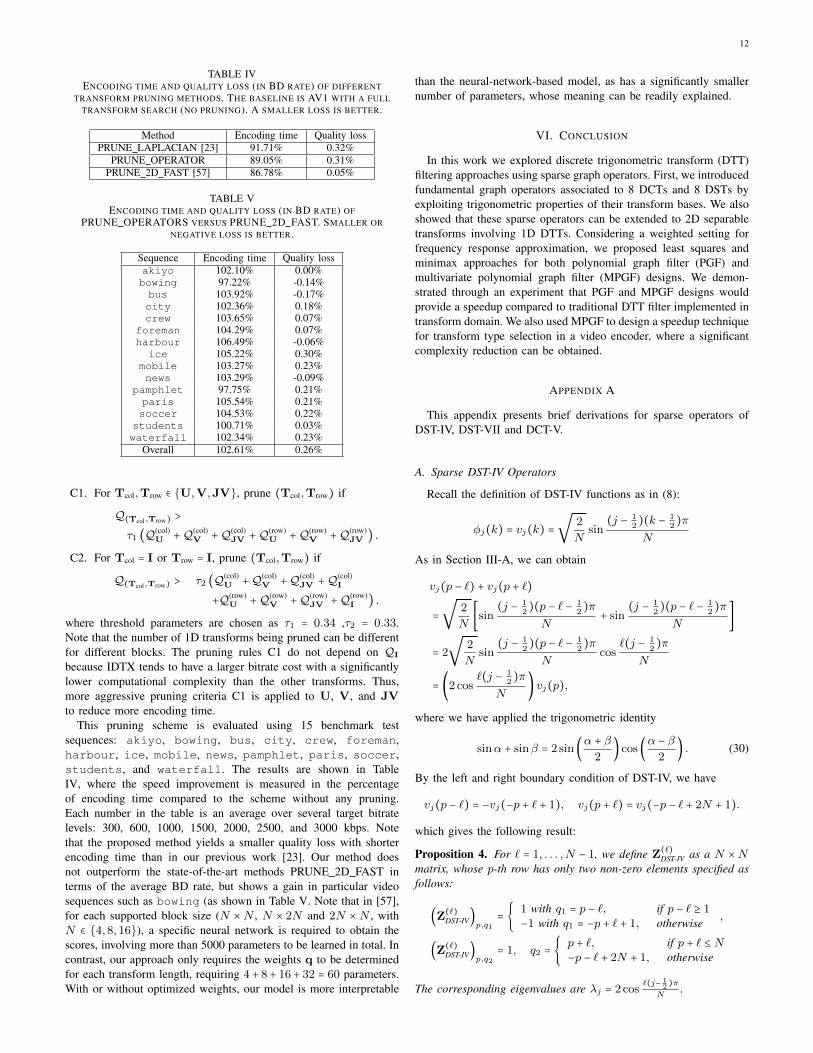
Method Encoding time Quality lossPRUNE LAPLACIAN [23] 91.71% 0.32%

PRUNE OPERATOR 89.05% 0.31%PRUNE 2D FAST [57] 86.78% 0.05%

TABLE VENCODING TIME AND QUALITY LOSS (IN BD RATE) OF

PRUNE OPERATORS VERSUS PRUNE 2D FAST. SMALLER ORNEGATIVE LOSS IS BETTER.

Sequence Encoding time Quality lossakiyo 102.10% 0.00%bowing 97.22% -0.14%bus 103.92% -0.17%city 102.36% 0.18%crew 103.65% 0.07%

foreman 104.29% 0.07%harbour 106.49% -0.06%ice 105.22% 0.30%

mobile 103.27% 0.23%news 103.29% -0.09%

pamphlet 97.75% 0.21%paris 105.54% 0.21%soccer 104.53% 0.22%students 100.71% 0.03%waterfall 102.34% 0.23%

Overall 102.61% 0.26%

C1. For Tcol,Trow ∈ {U,V,JV}, prune (Tcol,Trow) if

Q(Tcol,Trow) >

τ1 (Q(col)U +Q

(col)V +Q

(col)JV +Q

(row)U +Q

(row)V +Q

(row)JV ) .

C2. For Tcol = I or Trow = I, prune (Tcol,Trow) if

Q(Tcol,Trow) > τ2 (Q(col)U +Q

(col)V +Q

(col)JV +Q

(col)I

+Q(row)U +Q

(row)V +Q

(row)JV +Q

(row)I ) .

where threshold parameters are chosen as τ1 = 0.34 ,τ2 = 0.33.Note that the number of 1D transforms being pruned can be differentfor different blocks. The pruning rules C1 do not depend on QI

because IDTX tends to have a larger bitrate cost with a significantlylower computational complexity than the other transforms. Thus,more aggressive pruning criteria C1 is applied to U, V, and JVto reduce more encoding time.

This pruning scheme is evaluated using 15 benchmark testsequences: akiyo, bowing, bus, city, crew, foreman,harbour, ice, mobile, news, pamphlet, paris, soccer,students, and waterfall. The results are shown in TableIV, where the speed improvement is measured in the percentageof encoding time compared to the scheme without any pruning.Each number in the table is an average over several target bitratelevels: 300, 600, 1000, 1500, 2000, 2500, and 3000 kbps. Notethat the proposed method yields a smaller quality loss with shorterencoding time than in our previous work [23]. Our method doesnot outperform the state-of-the-art methods PRUNE 2D FAST interms of the average BD rate, but shows a gain in particular videosequences such as bowing (as shown in Table V. Note that in [57],for each supported block size (N ×N , N × 2N and 2N ×N , withN ∈ {4,8,16}), a specific neural network is required to obtain thescores, involving more than 5000 parameters to be learned in total. Incontrast, our approach only requires the weights q to be determinedfor each transform length, requiring 4+ 8+ 16+ 32 = 60 parameters.With or without optimized weights, our model is more interpretable

than the neural-network-based model, as has a significantly smallernumber of parameters, whose meaning can be readily explained.

VI. CONCLUSION

In this work we explored discrete trigonometric transform (DTT)filtering approaches using sparse graph operators. First, we introducedfundamental graph operators associated to 8 DCTs and 8 DSTs byexploiting trigonometric properties of their transform bases. We alsoshowed that these sparse operators can be extended to 2D separabletransforms involving 1D DTTs. Considering a weighted setting forfrequency response approximation, we proposed least squares andminimax approaches for both polynomial graph filter (PGF) andmultivariate polynomial graph filter (MPGF) designs. We demon-strated through an experiment that PGF and MPGF designs wouldprovide a speedup compared to traditional DTT filter implemented intransform domain. We also used MPGF to design a speedup techniquefor transform type selection in a video encoder, where a significantcomplexity reduction can be obtained.

APPENDIX A

This appendix presents brief derivations for sparse operators ofDST-IV, DST-VII and DCT-V.

A. Sparse DST-IV Operators

Recall the definition of DST-IV functions as in (8):

φj(k) = vj(k) =

√2

Nsin

(j − 12)(k − 1

2)π

N

As in Section III-A, we can obtain

vj(p − `) + vj(p + `)

=

√2

N[sin

(j − 12)(p − ` − 1

2)π

N+ sin

(j − 12)(p − ` − 1

2)π

N]

= 2

√2

Nsin

(j − 12)(p − ` − 1

2)π

Ncos

`(j − 12)π

N

= (2 cos`(j − 1

2)π

N) vj(p),

where we have applied the trigonometric identity

sinα + sinβ = 2 sin(α + β

2) cos(

α − β

2) . (30)

By the left and right boundary condition of DST-IV, we have

vj(p − `) = −vj(−p + ` + 1), vj(p + `) = vj(−p − ` + 2N + 1).

which gives the following result:

Proposition 4. For ` = 1, . . . ,N − 1, we define Z(`)DST-IV as a N ×N

matrix, whose p-th row has only two non-zero elements specified asfollows:

(Z(`)DST-IV)

p,q1= {

1 with q1 = p − `, if p − ` ≥ 1−1 with q1 = −p + ` + 1, otherwise

,

(Z(`)DST-IV)

p,q2= 1, q2 = {

p + `, if p + ` ≤ N−p − ` + 2N + 1, otherwise

The corresponding eigenvalues are λj = 2 cos`(j− 1

2)π

N.

13

B. Sparse DST-VII Operators

Now, we consider the basis function of DST-VII:

φj(k) =2

√2N + 1

sin(j − 1

2)kπ

N + 12

.

Then, by (30) we have

φj(p − `) + φj(p + `)

=2

√2N + 1

⎡⎢⎢⎢⎣sin

(j − 12) (p − `)π

N + 12

+ sin(j − 1

2) (p + `)π

N + 12

⎤⎥⎥⎥⎦

=2

√2N + 1

2 sin(j − 1

2)pπ

N + 12

cos` (j − 1

2)π

N + 12

=⎛

⎝2 cos

` (j − 12)π

N + 12

⎞

⎠φj(p) (31)

The left boundary condition (i.e., φj(k) = −φj(−k)) of DST-VIIcorresponds to φj(p − `) = −φj(−p + `). Together with the rightboundary condition φj(p + `) = φj(−p − ` + 2N + 1), we have thefollowing proposition.

Proposition 5. For ` = 1, . . . ,N − 1, we define Z(`)DST-VII as a N ×N

matrix, whose p-th row has at most two non-zero elements specifiedas follows:

(Z(`)DST-VII)

p,q1= {

1 with q1 = p − `, if p > `−1 with q1 = −p + `, if p < `

,

(Z(`)DST-VII)

p,q2= 1, q2 = {

p + `, if p + ` ≤ N−p − ` + 2N + 1, otherwise

The corresponding eigenvalues are λj = 2 cos`(j− 1

2)π

N+ 12

.

In Proposition 5, note that the `-th row has only one nonzeroelement because when p = `, φj(p − `) = 0, and (31) reduces to

φj(p + `) =⎛

⎝2 cos

` (j − 12)π

N + 12

⎞

⎠φj(p).

C. Sparse DCT-V Operators

Here, φj are defined as DCT-V basis functions

φj(k) =2

√2N − 1

cjck sin(j − 1)(k − 1)π

N − 12

.

Note that ck = 1/√2 for k = 1 and 1 otherwise. For the trigonometric

identity (15) to be applied, we introduce a scaling factor such thatbkck = 1 for all k:

bk = {

√2, k = 1

1, otherwise.

In this way, by (15) we have

bp−` ⋅ φj(p − `) + bp+` ⋅ φj(p + `)

=2

√2N − 1

cj [cos(j − 1)(p − ` − 1)π

N − 12

+ cos(j − 1)(p + ` − 1)π

N − 12

]

=2

√2N − 1

cj2 cos(j − 1)(p − 1)π

N − 12

cos`(j − 1)π

N − 12

= (2 cos`(j − 1)π

N − 12

) bpφj(p),

so this eigenvalue equation can be written as

bp−`bp

⋅φj(p− `)+bp+`bp

⋅φj(p+ `) = (2 cos`(j − 1)π

N − 12

)φj(p). (32)

The left boundary condition of DCT-V corresponds to φj(p− `) =φj(−p + ` + 2), and the right boundary condition gives φj(p + `) =φj(−p − ` + 2N + 1). Thus, (32) yields the following proposition:

Proposition 6. For ` = 1, . . . ,N − 1, we define Z(`)DCT-V as a N ×N

matrix, whose p-th row has at most two non-zero elements specifiedas follows:

(Z(`)DCT-V)

p,q1=

⎧⎪⎪⎪⎨⎪⎪⎪⎩

√2 with q1 = 1, if p − ` = 1

1 with q1 = p − `, if p − ` > 11 with q1 = −p + ` + 2, if p − ` ≤ 0, p ≠ 1

,

(Z(`)DCT-V)

p,q2=

⎧⎪⎪⎪⎨⎪⎪⎪⎩

√2 with q2 = 1, p = 1

1 with q2 = p + `, p ≠ 1, p + ` ≤ N1 with q2 = −p − ` + 2N + 1, otherwise

The corresponding eigenvalues are λj = 2 cos `(j−1)πN− 1

2

.

The values of√2 in Proposition 6 arise from bp−`/bp and bp+`/bp

in the LHS of (32). In particular, when p = `+1 we have bp−`/bp =√2

and bp+`/bp = 1, so (32) gives

√2φj(p − `) + φj(p + `) = (2 cos

`(j − 1)π

N − 12

)φj(p).

When p = 1, bp−`/bp = bp+`/bp = 1/√2. In addition, by the left

boundary condition, φj(p − `) = φj(p + `), so (32) reduces to

√2φj(p + `) = (2 cos

`(j − 1)π

N − 12

)φj(p), for p = 1.

meaning that the first row of Z(`)DCT-V has one nonzero element only.

APPENDIX B

This appendix includes remarks on the retrieval of sparse operatorsfor general GFTs beyond DCT and DST.

The characterization of all Laplacians that share a common GFThas been studied in the context of graph topology identification andgraph diffusion process inference [47], [59], [60]. In particular, it hasbeen shown in [47] that the set of normalized Laplacian matriceshaving a fixed GFT can be characterized by a convex polytope.Following a similar proof, we briefly present the counterpart resultfor unnormalized Laplacian with self-loops allowed:

Theorem 1. The set of Laplacian matrices with a fixed GFT can becharacterized by a convex polyhedral cone in the space of eigenvalues(λ1, . . . , λN).

Proof: For a given GFT Φ, let the eigenvalues λj of the Laplacianbe variables. By definition of the Laplacian (4), we can see that

L = Φ ⋅ diag(λ1, . . . , λN) ⋅Φ⊺=

N

∑k=1

λkφkφ⊺k (33)

is a valid Laplacian matrix if lij ≤ 0 (non-negative edge weights),lii ≥ ∑

Nj=1,j≠i lij (non-negative self-loop weights), and λk ≥ 0 for

all k (non-negative graph frequencies). With the expression (33) wehave lij = ∑

Nk=1 λkφk(i)φk(j), and thus the Laplacian conditions

can be expressed in terms of λj’s:

N

∑k=1

λkφk(i)φk(j) ≤ 0, for i ≠ j,

N

∑k=1

λkφk(i)2≥N

∑j=1j≠i

λkφk(i)φk(j), for i = 1, . . . ,N,

λk ≥ 0, k = 1, . . . ,N. (34)

14

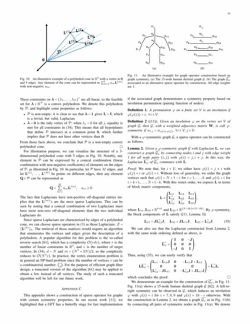
Fig. 10. An illustrative example of a polyhedral cone in R3 with a vertex at 0and 5 edges. Any element of the cone can be represented as ∑5

m=1 amL(m)

with non-negative am.

These constraints on λ = (λ1, . . . , λN)⊺ are all linear, so the feasible

set for λ ∈ RN is a convex polyhedron. We denote this polyhedronby P , and highlight some properties as follows:

● P is non-empty: it is clear to see that λ = 1 gives L = I, whichis a trivial, but valid, Laplacian.

● λ = 0 is the only vertex of P: when λj = 0 for all j, equality ismet for all constraints in (34). This means that all hyperplanesthat define P intersect at a common point 0, which furtherimplies that P does not have other vertices than 0.

From those facts above, we conclude that P is a non-empty convexpolyhedral cone.

For illustration purpose, we can visualize the structure of a 3-dimensional polyhedral cone with 5 edges in Fig. 10. Notably, anyelement in P can be expressed by a conical combination (linearcombination with non-negative coefficients) of elements on the edgesof P , as illustrated in Fig. 10. In particular, let P have M edges, andlet L(1), . . . , L(M) be points on different edges, then any elementQ ∈ P can be represented as

Q =M

∑m=1

amL(m), am ≥ 0.

The fact that Laplacians have non-positive off-diagonal entries im-plies that the L(m)’s are the most sparse Laplacians. This can beseen by noting that a conical combination of two Laplacians musthave more non-zero off-diagonal elements than the two individualLaplacians do.

Since sparse Laplacians are characterized by edges of a polyhedralcone, we can choose sparse operators in (3) as those Laplacians: Z =

{L(k)}k. The retrieval of those matrices would require an algorithmthat enumerates the vertices and edges given the description of apolyhedron. A popular algorithm for this problem is the so-calledreverse search [61], which has a complexity O(rdv), where r is thenumber of linear constraints in Rd, and v is the number of targetvertices. In (34), d = N and m = (N2

+ 3N)/2, so the complexityreduces to O(N3v). In practice, the vertex enumeration problem isin general an NP-hard problem since the number of vertices v can bea combinatorial number: (r

d). For the purpose of efficient graph filter

design, a truncated version of the algorithm [61] may be applied toobtain a few instead of all vertices. The study of such a truncatedalgorithm will be left for our future work.

APPENDIX C

This appendix shows a construction of sparse operator for graphswith certain symmetry properties. In our recent work [11], wehighlighted that a GFT has a butterfly stage for fast implementation

(a) (b)

Fig. 11. An illustrative example for graph operator construction based ongraph symmetry. (a) The 15-node human skeletal graph G. (b) The graph Gϕassociated to an alternative sparse operator by construction. All edge weightsare 1.

if the associated graph demonstrates a symmetry property based oninvolution permutation (pairing function of nodes):

Definition 1. A permutation ϕ on a finite set V is an involution ifϕ(ϕ(i)) = i, ∀i ∈ V .

Definition 2 ([11]). Given an involution ϕ on the vertex set V ofgraph G, then G, with a weighted adjacency matrix W, is call ϕ-symmetric if wi,j = wϕ(i),ϕ(j), ∀i ∈ V, j ∈ V .

With a ϕ-symmetric graph G, a sparse operator can be constructedas follows.

Lemma 2. Given a ϕ-symmetric graph G with Laplacian L, we canconstruct a graph Gϕ by connecting nodes i and j with edge weight1 for all node pairs (i, j) with ϕ(i) = j, i ≠ j. In this way, theLaplacian Lϕ of Gϕ commutes with L.

Proof: We note that, for i ∈ V , we either have ϕ(i) = j ≠ i withϕ(j) = i or ϕ(i) = i. Without loss of generality, we order the graphvertices such that ϕ(i) = N + 1 − i for i = 1, . . . , k and ϕ(i) = i fori = k+1, . . . ,N +1−k. With this vertex order, we express L in termsof block matrix components,

L =⎛⎜⎝

L11 L12 L13

L⊺12 L22 L23

L⊺13 L⊺

23 L33

⎞⎟⎠,

where L11,L33 ∈ Rk×k and L22 ∈ R(N−2k)×(N−2k). By ϕ-symmetry,the block components of L satisfy ([11, Lemma 3])

L13 = JL⊺13J, L33 = JL11J, L23 = L⊺

12J. (35)

We can also see that the Laplacian constructed from Lemma 2,with the same node ordering defined as above, is

Lϕ =⎛⎜⎝

I 0 −J0 0 0−J 0 I

⎞⎟⎠.

Then, using (35), we can easily verify that

LLϕ =⎛⎜⎝

L11 −L13J 0 −L11J +L13

0 0 0L⊺

13 − JL11 0 −L⊺13J + JL11J

⎞⎟⎠= LϕL,

which concludes the proof.We demonstrate an example for the construction of Gϕ, in Fig. 11.

Fig. 11(a) shows a 15-node human skeletal graph G [62]. A left-to-right symmetry can be observed in G, which induces an involutionϕ with ϕ(i) = i for i = 7,8,9 and ϕ(i) = 16 − i otherwise. Withthe construction in Lemma 2, we obtain a graph Gϕ as in Fig. 11(b)by connecting all pairs of symmetric nodes in Fig. 11(a). We denote

15

Z(1) = L and Z(2) = Lϕ the Laplacians of G and Gϕ, respectively,and Ψ = (ψ1, . . . ,ψ15) the GFT matrix of L with basis functionsin increasing order of eigenvalues. In particular, we have

Z(2) = Ψ ⋅ diag(λ(2)) ⋅Ψ⊺,

λ(2) = (0,0,2,2,0,0,0,2,2,0,0,2,2,0,0)⊺.

Since Z(2) has only two distinct eigenvalues with high multiplicities,every polynomial of Z(2) also has two distinct eigenvalues only,which poses a limitation for graph filter design. However, an MPGFwith both Z(1) and Z(2) still provides more degrees of freedomcompared to a PGF with a single operator.

REFERENCES

[1] A. Sandryhaila and J.M.F. Moura, “Discrete signal processing ongraphs,” Signal Processing, IEEE Trans. on, vol. 61, no. 7, pp. 1644–1656, Apr. 2013.

[2] D. I. Shuman, S. K. Narang, P. Frossard, A Ortega, and P. Vandergheynst,“The emerging field of signal processing on graphs: Extending high-dimensional data analysis to networks and other irregular domains,”Signal Processing Magazine, IEEE, vol. 30, no. 3, pp. 83–98, May 2013.

[3] A. Ortega, P. Frossard, J. Kovacevic, J. M. F. Moura, and P. Van-dergheynst, “Graph signal processing: Overview, challenges, and ap-plications,” Proceedings of the IEEE, vol. 106, no. 5, pp. 808–828, May2018.

[4] S. Chen, A. Sandryhaila, J. M. F. Moura, and J. Kovacevic, “Signal de-noising on graphs via graph filtering,” in 2014 IEEE Global Conferenceon Signal and Information Processing (GlobalSIP), 2014, pp. 872–876.

[5] M. Onuki, S. Ono, M. Yamagishi, and Y. Tanaka, “Graph signaldenoising via trilateral filter on graph spectral domain,” IEEE Trans.on Signal and Information Processing over Networks, vol. 2, no. 2, pp.137–148, June 2016.

[6] A. C. Yagan and M. T. Ozgen, “A spectral graph wiener filter in graphfourier domain for improved image denoising,” in 2016 IEEE GlobalConference on Signal and Information Processing (GlobalSIP), 2016,pp. 450–454.

[7] J. Ma, W. Huang, S. Segarra, and A. Ribeiro, “Diffusion filtering ofgraph signals and its use in recommendation systems,” in 2016 IEEEInternational Conference on Acoustics, Speech and Signal Processing(ICASSP), 2016, pp. 4563–4567.

[8] N. Tremblay, G. Puy, R. Gribonval, and P. Vandergheynst, “Compressivespectral clustering,” in Proceedings of the 33rd International Conferenceon International Conference on Machine Learning - Volume 48. 2016,ICML’16, p. 1002–1011, JMLR.org.

[9] T. N. Kipf and M. Welling, “Semi-Supervised Classification with GraphConvolutional Networks,” arXiv:1609.02907 [cs, stat], Feb. 2017, arXiv:1609.02907.

[10] M. Defferrard, X. Bresson, and P. Vandergheynst, “Convolutional neuralnetworks on graphs with fast localized spectral filtering,” in Proceedingsof the 30th International Conference on Neural Information ProcessingSystems, Red Hook, NY, USA, 2016, NIPS’16, p. 3844–3852, CurranAssociates Inc.

[11] K.-S. Lu and A. Ortega, “Fast graph Fourier transforms based on graphsymmetry and bipartition,” IEEE Trans. on Signal Processing, vol. 67,no. 18, pp. 4855–4869, 2019.

[12] E. Isufi, A. Loukas, A. Simonetto, and G. Leus, “Autoregressive movingaverage graph filtering,” IEEE Trans. on Signal Processing, vol. 65, no.2, pp. 274–288, Jan 2017.

[13] M. Coutino, E. Isufi, and G. Leus, “Advances in distributed graphfiltering,” IEEE Trans. on Signal Processing, vol. 67, no. 9, pp. 2320–2333, May 2019.

[14] N. Tremblay, P. Goncalves, and P. Borgnat, “Design of graph filter andfilterbanks,” in Cooperative and Graph Signal Processing, pp. 299–324.Academic Press, June 2018.

[15] A. Sandryhaila and J.M.F. Moura, “Discrete signal processing on graphs:Frequency analysis,” Signal Processing, IEEE Trans. on, vol. 62, no.12, pp. 3042–3054, June 2014.

[16] A. Ortega, Introduction to Graph Signal Processing, CambridgeUniversity Press, 2021.

[17] D. K. Hammond, P. Vandergheynst, and R. Gribonval, “Wavelets ongraphs via spectral graph theory,” Applied and Computational HarmonicAnalysis, vol. 30, no. 2, pp. 129–150, 2011.

[18] D. I. Shuman, P. Vandergheynst, D. Kressner, and P. Frossard, “Dis-tributed signal processing via Chebyshev polynomial approximation,”IEEE Trans. on Signal and Information Processing over Networks, vol.4, no. 4, pp. 736–751, Dec 2018.

[19] S. Segarra, A. G. Marques, and A. Ribeiro, “Optimal graph-filter designand applications to distributed linear network operators,” IEEE Trans.on Signal Processing, vol. 65, no. 15, pp. 4117–4131, Aug 2017.

[20] A. Loukas, A. Simonetto, and G. Leus, “Distributed autoregressivemoving average graph filters,” IEEE Signal Processing Letters, vol.22, no. 11, pp. 1931–1935, 2015.

[21] J. Liu, E. Isufi, and G. Leus, “Filter design for autoregressive moving av-erage graph filters,” IEEE Trans. on Signal and Information Processingover Networks, vol. 5, no. 1, pp. 47–60, July 2019.

[22] A. Gavili and X. Zhang, “On the shift operator, graph frequency, andoptimal filtering in graph signal processing,” IEEE Trans. on SignalProcessing, vol. 65, no. 23, pp. 6303–6318, Dec 2017.

[23] K.-S. Lu, A. Ortega, D. Mukherjee, and Y. Chen, “Efficient rate-distortion approximation and transform type selection using Laplacianoperators,” in 2018 Picture Coding Symposium (PCS), June 2018, pp.76–80.

[24] N. Emirov, C. Cheng, J. Jiang, and Q. Sun, “Polynomial graph filterof multiple shifts and distributed implementation of inverse filtering,”arXiv:2003.11152, March 2020.

[25] G. Strang, “The discrete cosine transform,” SIAM review, vol. 41, no.1, pp. 135–147, 1999.

[26] M. Puschel and J. M. F Moura, “The algebraic approach to the discretecosine and sine transforms and their fast algorithms,” SIAM Journal onComputing, vol. 32, no. 5, pp. 1280–1316, 2003.

[27] W. H. Chen and S. C. Fralick, “Image enhancement using cosinetransform filtering,” in Image Sci. Math. Symp., Nov 1976.

[28] Y. Park and H. Park, “Design and analysis of an image resizing filterin the block-DCT domain,” IEEE Trans. on Circuits and Systems forVideo Technology, vol. 14, no. 2, pp. 274–279, 2004.

[29] H. S. Shin, C. Lee, and M. Lee, “Ideal filtering approach on DCT domainfor biomedical signals: index blocked dct filtering method (ib-dctfm),”J. Med. Syst., vol. 34, no. 2, pp. 741–753, Aug. 2010.

[30] U. Tuna, S. Peltonen, and U. Ruotsalainen, “Gap-filling for the high-resolution pet sinograms with a dedicated DCT-domain filter,” IEEETrans. on Medical Imaging, vol. 29, no. 3, pp. 830–839, 2010.

[31] C. Zhang, D. Florencio, and P. A. Chou, “Graph signal processing–aprobabilistic framework,” Technical Report, Apr 2015.

[32] B. Chitprasert and K. R. Rao, “Discrete cosine transform filtering,”Signal Processing, vol. 19, no. 3, pp. 233–245, 1990.

[33] S. A. Martucci, “Symmetric convolution and the discrete sine and cosinetransforms,” IEEE Trans. on Signal Processing, vol. 42, no. 5, pp. 1038–1051, 1994.

[34] W. Hu, G. Cheung, A. Ortega, and O. C. Au, “Multiresolution graphFourier transform for compression of piecewise smooth images,” IEEETrans. on Image Processing, vol. 24, no. 1, pp. 419–433, Jan 2015.

[35] G. Fracastoro, D. Thanou, and P. Frossard, “Graph transform optimiza-tion with application to image compression,” IEEE Trans. on ImageProcessing, vol. 29, pp. 419–432, 2020.

[36] Z. Wang and B.R. Hunt, “The discrete W transform,” AppliedMathematics and Computation, vol. 16, no. 1, pp. 19 – 48, 1985.

[37] J. Han, A. Saxena, V. Melkote, and K. Rose, “Jointly optimized spatialprediction and block transform for video and image coding,” IEEETrans. Image Process., vol. 21, no. 4, pp. 1874–1884, Apr 2012.

[38] W. Hu, G. Cheung, and A. Ortega, “Intra-prediction and generalizedgraph Fourier transform for image coding,” Signal Processing Letters,IEEE, vol. 22, no. 11, pp. 1913–1917, Nov. 2015.

[39] J. Han, Y. Xu, and D. Mukherjee, “A butterfly structured design of thehybrid transform coding scheme,” in Picture Coding Symposium, 2013,pp. 1–4.

[40] Y. Chen, D. Mukherjee, J. Han, A. Grange, Y. Xu, S. Parker, C. Chen,H. Su, U. Joshi, C.-H. Chiang, and et al., “An overview of coding toolsin av1: the first video codec from the alliance for open media,” APSIPATrans. on Signal and Information Processing, vol. 9, pp. e6, 2020.

[41] T. Hofmann, B. Scholkopf, and A. J. Smola, “Kernel methods in machinelearning,” Annals of Statistics, vol. 36, no. 3, pp. 1171–1220, 2008.

[42] H. Kitajima, “A symmetric cosine transform,” IEEE Trans. onComputers, vol. C-29, no. 4, pp. 317–323, Apr. 1980.

[43] H. Hou, “A fast recursive algorithm for computing the discrete cosinetransform,” IEEE Trans. on Acoustics, Speech, and Signal Processing,vol. 35, no. 10, pp. 1455–1461, 1987.

[44] V. Sanchez, P. Garcia, A. M. Peinado, J. C. Segura, and A. J. Rubio,“Diagonalizing properties of the discrete cosine transforms,” IEEETrans. on Signal Processing, vol. 43, no. 11, pp. 2631–2641, 1995.

16

[45] H. Zhang and F. Ding, “On the Kronecker products and their applica-tions,” Journal of Applied Mathematics, vol. 2013, 06 2013.

[46] B. Mohar, “The Laplacian spectrum of graphs,” in Graph Theory,Combinatorics, and Applications. 1991, pp. 871–898, Wiley.

[47] B. Pasdeloup, V. Gripon, G. Mercier, D. Pastor, and M. G. Rabbat,“Characterization and inference of graph diffusion processes from ob-servations of stationary signals,” IEEE Trans. on Signal and InformationProcessing over Networks, vol. 4, no. 3, pp. 481–496, Sep. 2018.

[48] Y. C. Pati, R. Rezaiifar, and P. S. Krishnaprasad, “Orthogonal matchingpursuit: Recursive function approximation with applications to waveletdecomposition,” in Proceedings of the 27th Annual Asilomar Conferenceon Signals, Systems, and Computers, 1993, pp. 40–44.

[49] R. Tibshirani, “Regression shrinkage and selection via the lasso,”Journal of the Royal Statistical Society (Series B), vol. 58, pp. 267–288, 1996.

[50] J. McClellan, T. Parks, and L. Rabiner, “A computer program fordesigning optimum FIR linear phase digital filters,” IEEE Trans. onAudio and Electroacoustics, vol. 21, no. 6, pp. 506–526, 1973.

[51] K.-S. Lu, “Sparse DTT operators,” [online] https://github.com/kslu/sparseDttOperators.

[52] O. Teke and P. P. Vaidyanathan, “Extending classical multirate signalprocessing theory to graphs-Part II: M-channel filter banks,” IEEE Trans.on Signal Processing, vol. 65, no. 2, pp. 423–437, Jan 2017.

[53] Y. Tanaka and A. Sakiyama, “M -channel oversampled graph filterbanks,” IEEE Trans. on Signal Processing, vol. 62, no. 14, pp. 3578–3590, 2014.

[54] W.-H. Chen, C. Smith, and S. Fralick, “A fast computational algorithmfor the discrete cosine transform,” IEEE Trans. on Communications, vol.25, no. 9, pp. 1004–1009, 1977.

[55] A. Smola and R. Kondor, “Kernels and regularization on graphs,” inLearning Theory and Kernel Machines, Jan 2003, vol. 2777, pp. 144–158.

[56] V. K. Goyal, “Theoretical foundation of transform coding,” IEEE SignalProcessing Magazine, pp. 9–21, Sept 2001.

[57] H. Su, M. Chen, A. Bokov, D. Mukherjee, Y. Wang, and Y. Chen,“Machine learning accelerated transform search for AV1,” in 2019Picture Coding Symposium (PCS), 2019, pp. 1–5.

[58] B. Li, J. Han, and Y. Xu, “Fast transform type selection using conditionalLaplacian distribution based rate estimation,” in Applications of DigitalImage Processing XLIII, Andrew G. Tescher and Touradj Ebrahimi, Eds.International Society for Optics and Photonics, 2020, vol. 11510, pp.461–468, SPIE.

[59] S. Segarra, A. G. Marques, G. Mateos, and A. Ribeiro, “Networktopology inference from spectral templates,” IEEE Trans. on Signaland Information Processing over Networks, vol. 3, no. 3, pp. 467–483,Sep. 2017.

[60] Y. De Castro, T. Espinasse, and P. Rochet, “Reconstructing undirectedgraphs from eigenspaces,” J. Mach. Learn. Res., vol. 18, no. 1, pp.1679–1702, Jan. 2017.

[61] D. Avis and F. Fukuda, “A pivoting algorithm for convex hulls and vertexenumeration of arrangements and polyhedra,” Discrete & ComputationalGeometry, vol. 8, pp. 295–313, Sep 1992.

[62] J.-Y. Kao, A. Ortega, and S. S. Narayanan, “Graph-based approachfor motion capture data representation and analysis,” in 2014 IEEEInternational Conference on Image Processing (ICIP), Oct 2014, pp.2061–2065.