Growing like China�
Zheng SongFudan University
Kjetil StoreslettenUniversity of Oslo and CEPR
Fabrizio ZilibottiUniversity of Zurich and CEPR
First version: March 2008This version: December 2008
Abstract
China has been growing at a high rate and has at the same time accumulated a stag-gering foreign surplus. We constructs a theory that explain these seemingly puzzling ob-servations, while being consistent with salient features of the Chinese growth experiencesince 1992: high output growth, sustained returns on capital investments, extensive real-location within the manufacturing sector, falling labor share and accumulation of a largeforeign surplus. The theory makes only minimal deviations from a neoclassical growthmodel. Its building blocks are �nancial imperfections and reallocation among �rms withheterogeneous productivity. Some �rms use more productive technologies than others, butlow-productivity �rms survive because of better access to credit markets. Due to the �-nancial imperfections, high-productivity �rms �which are run by entrepreneurs �must be�nanced out of internal savings. If these savings are su¢ ciently large, the high-productivitysector outgrows the low-productivity sector, and attracts an increasing employment share.During the transition, low wage growth sustains the return to capital. The downsizing ofthe �nancially integrated sector forces a growing share of domestic savings to be investedin foreign assets, generating a foreign surplus. We test some auxiliary implications of thetheory and �nd robust empirical support.JEL No .G18, O11, O16, O47, O53, P31.Keywords: China, Economic Growth, Entrepreneurs, Financial Market Imperfections,
Foreign Surplus, Investment, Loans, Productivity Heterogeneity, Rate of Return on Capital,Reallocation, State-Owned Firms.
�We thank seminar participants at Columbia University, CREi, Chinese University of Hong Kong, LondonSchool of Economics (conference "The Emergence of China & India in the Global Economy", 3-5 July 2008),Universitat Autonoma, University of Oslo, University of Zurich and WISE for comments. Financial supportfrom the European Research Council (ERC Advanced Grant IPCDP-229883) is gratefully acknowledged.
1

1 Introduction
Over the last thirty years, China has undergone a spectacular economic transformation.
The transformation has involved not only fast economic growth and sustained capital
accumulation, but also major shifts in the sectoral composition of output, urbanization,
and a growing importance of markets and entrepreneurial skills. Reallocation of both
labor and capital across manufacturing �rms has been a key source of productivity
growth. The rate of return on investments has remained well above 20%, higher than
in most industrialized and developing economies. If investment rates have been high,
saving rates have been even higher: in the last �fteen years, China has seen a growing
net foreign surplus. Its foreign reserves swelled from 21 billion USD in 1992 (5% of its
GDP) to 1700 billion USD in March 2008 (43% of its GDP), see Figure 1.
FIGURE 1 HERE
The joint observation of high growth and high return on capital, on the one hand,
combined with a growing foreign surplus, on the other hand, is puzzling. A closed-
economy neoclassical growth model would predict that the high investment rate should
lead to a substantial fall in the return to capital. An open-economy model would predict
a large net capital in�ow rather than an out�ow, owing to the high domestic return on
capital. In this paper, we propose a theory of economic transition that resolves this
puzzle while being consistent with the main stylized facts of the Chinese experience. The
focal points of the theory are �nancial frictions and �rms�reallocation. In our theory,
both the sustained return on capital and the foreign surplus arise from the reallocation
of capital and labor from less productive externally-�nanced �rms to entrepreneurial
�rms that are more productive, but have less access to external �nancing. As �nancially
integrated �rms shrink, a larger proportion of the domestic savings is invested in foreign
assets. Thus, high growth and high investments are consistent with the accumulation of
a foreign surplus.
Our paper is part of a recent literature arguing that low aggregate total factor pro-
ductivity (TFP) � especially in developing countries � is the result of micro-level re-
source misallocation (see Parente, Rogerson and Wright, 2000, Caselli and Coleman
2002, Banerjee and Du�o 2005, Hsieh and Klenow, 2007, Restuccia and Rogerson, 2008,
1
Page 2 of 53

and Gancia and Zilibotti, 2009). While pockets of e¢ cient �rms using state-of-art tech-
nologies may exist, these �rms fail to attract the large share of productive resources that
e¢ ciency would dictate, due to �nancial frictions and other imperfections. Most existing
literature emphasizes the e¤ects of resource misallocation on average productivity. In
contrast, our paper argues that when a country starts from a situation of severe ine¢ -
ciency, but manages to ignite the engine of reallocation, it has the potential to grow fast
over a prolonged transition. The mechanism is similar to that of models of transition
from agriculture to industry (see Lewis (1954) and more discussion below): e¢ cient �rms
can count on a highly elastic supply of factors attracted from the less productive �rms.
To analyze such transition, we construct a model where �rms are heterogeneous in
productivity and access to �nancial markets. High-productivity �rms are operated by
agents with entrepreneurial skills who are �nancially constrained and who must rely on
retained earnings to �nance their investments. Low-productivity �rms can survive due to
their better access to credit markets, since the growth potential of high-productivity �rms
is limited by the extent of entrepreneurial savings. If the saving �ow is su¢ ciently large,
high-productivity �rms outgrow low-productivity ones, progressively driving them out of
the market. During the transition, the dynamic equilibrium has "AK" features: within
each sector, the rate of return to capital is constant due to labor mobility and to the
�nancial integration of one of the two sectors. Due to a composition e¤ect, the aggregate
rate of return on capital actually increases. Moreover, the economy accumulates a foreign
surplus. While investments in the expanding sector are �nanced by the retained earnings
of entrepreneurs, wage earners deposit their savings with intermediaries who can invest
them in loans to domestic �rms and in foreign bonds. As the demand for funds from
�nancially-integrated domestic �rms declines, a growing share of the intermediated funds
must be invested abroad, building a growing foreign surplus. This prediction is consistent
with the observation that the di¤erence between deposits and domestic bank loans has
been growing substantially, tracking China�s accumulation of foreign reserves (see again
Figure 1). After the transition, the economy behaves as in a standard neoclassical model
where capital accumulation is subject to decreasing returns.
Reallocation within the manufacturing sector �the driving force in our model �has
been shown to be a source of �rst-order productivity growth in China. In an in�uential
paper, Hsieh and Klenow (2007) estimate that reallocation across manufacturing �rms
with di¤erent productivity accounts for an annual 1.4 percentage points increase in
aggregate TFP during 1998-2005. Thus, reallocation may account for a large share of
2
Page 3 of 53
total TFP growth.1
Our theory bears a number of auxiliary predictions that are consistent with the
evidence of China�s transition. We state here the main implications, and defer a more
detailed discussion of the evidence to section 2.
1. The theory predicts that savings determine investments in regions with a high
intensity of entrepreneurial �rms, while investments are unrelated to savings in
regions dominated by �nancially-integrated �rms. Consistent with this prediction,
we �nd the time-series correlation between investments and savings to be signi�-
cantly higher in Chinese provinces with a high employment share in entrepreneurial
�rms.
2. In the benchmark model, all �rms produce the same good and di¤er only in TFP.
We extend the theory to a two-sector model where �rms can specialize in the pro-
duction of more or less capital-intensive goods. This extension bears the prediction
that �nancially constrained �rms with high TFP will specialize in labor-intensive
activities (even though they have no technological comparative advantage). Thus,
the transition proceeds in stages: �rst low-productivity �rms retreat to capital-
intensive industries, and then they gradually vanish. This is consistent with the
observed dynamics of sectoral reallocation in China, where young high-productivity
private �rms have entered extensively in labor-intensive sectors, while old state-
owned �rms continue to dominate capital-intensive industries.
3. The theory predicts rising inequality within urban areas, as wages grow less than
entrepreneurial rents during the transition. Moreover, inequality should be higher
in regions with a high density of entrepreneurial activity. We �nd both predictions
to be consistent with the evidence for China.
The theory is related to the seminal work of Kuznets (1966) and Chenery and Syrquin
(1975) who study sources of productivity growth during economic transitions. In the
same vein, Lewis (1954) constructs a model of reallocation from agriculture to industry
where the supply of labor in manufacturing is "unlimited" due to structural overem-
ployment in agriculture. While his mechanism is similar in some respects with ours,
productivity increases in his model rely on some form of hidden unemployment in the
traditional sector. Lewis�theory captures aspects of the reallocation between rural and
1Recent papers estimate the annual TFP growth in the manufacturing sector to be in the rangebetween 1.4%-3% (Wang and Yao 2001, Young 2003, Islam et al., 2006).
3
Page 4 of 53
urban areas in China, while our focus is on the reallocation within the industrial sector
and on the accumulation of foreign reserves. Other papers focusing on the transition
from agriculture to industry include Fei and Ranis (1961 and 1964), Takayama (1965),
Laitner (1990) and Matsuyama (1992).
Our paper is also related to Ventura (1997), who shows that in economies engaging in
external trade capital accumulation is not subject to diminishing returns since resources
are moved from labor-intensive to capital-intensive sectors. Due to international trade,
the growing production of capital goods is exported, thus preventing the returns to
capital from falling. Ventura�s model does not assume any initial ine¢ ciency, nor does
it imply that TFP should grow within each industry �a key implication of our theory.
In addition, his model has no implications regarding trade imbalances.
Matsuyama (2004, 2005) show that �nancial frictions may induce trading economies
to specialize in industries where they do not have a technological comparative advantage.
In our model, by a similar mechanism, less e¢ cient �rms can survive and even outgrow
more productive ones. Moreover, our two-sector extension also predicts that �nancial
constraints generate specialization in spite of the lack of any technological comparative
advantage. Matsuyama (2007) provides a survey of the literature on economic transition.
Gourinchas and Jeanne (2007) note �as we do in this paper �that the observation
that capital tend to �ow out of fast-growing economies with high marginal product of
capital is inconsistent with the neoclassical growth model. They show, using a panel of
69 developing countries, that this pattern is not a unique feature of China. In particular,
developing countries with fast TFP growth tend to have both large capital out�ows and
large investment rates, while the opposite is true for slow-growing countries. They label
this �nding as the �allocation puzzle�.
A few recent papers address the more speci�c question of why China is accumulating
a large foreign surplus. Most papers emphasize the country�s high saving rate. Kuijs
(2005) shows that household and enterprise saving rates in China are, respectively, 11.8
and 8.6 percentage points higher than those in the US, respectively. Demography, the
lack of social security and an imperfect �nancial sector are among the factors proposed
as explanations for this (e.g. Kraay, 2000). However, it remains unclear why domestic
savings are not invested domestically given the high rate of return to capital in China.
Mendoza, Quadrini and Rios-Rull (2007) argue that this may be explained by di¤erences
in �nancial development inducing savers in emerging economies to seek insurance in safe
US bonds (see also Caballero, Farhi and Gourinchas, 2006). Dooley, Folkerts-Landau
and Garber (2004) propose a strategic "political" motive: the Chinese government would
4
Page 5 of 53

in�uence wages, interest rates and international �nancial transactions so as to foster
employment and export-led growth.
The paper is organized as follows. Section 2 describes some empirical evidence for
China since 1992 that motivates our analysis. Section 3 describes the benchmark model
and characterizes equilibrium. Section 4 discusses the e¤ect of �nancial development.
Section 5 presents two extensions focusing, respectively, on regional shocks to savings
and on specialization of di¤erent �rms in labor- or capital-intensive production. Section
6 concludes. Proofs and other technical material are contained in an appendix
2 The transition of China: empirical evidence
After thirty years of central planning, China introduced its �rst economic reforms in
December 1978. The early reforms reduced land collectivization introducing the principle
of household responsibility in agriculture, increased the role of local governments and
communities, and experimented with market reforms in a few selected special economic
zones. During the 1980s, China was a mixed economy, with some elements of planning
and others of market economy, and with a high but volatile growth.
After a period of economic and political instability, a new stage of the reform process
began in 1992, inaugurated by Deng Xiaoping�s "southern tour" during which the leader
spoke in favor of an acceleration of reforms (see Zhao 1993). Since then, China has moved
towards a fully-�edged market economy. Thereafter, the role of the state in allocating
resources has decreased, and many unpro�table enterprises were shut down. The focus
of this paper is on the post-1992 Chinese transition, a period characterized by a fast
and stable growth, and by a pronounced resource reallocation within the manufacturing
sector. In spite of very high investment rates (37% on average), the rate of return to
capital has not fallen over time, especially in the manufacturing sector. If the aggregate
return to capital fell slightly (from 28% in 1993 to 21% in 2005), the rate of return on
capital in manufacturing has been increasing over time since the early 1990s and climbed
close to 35% in 2003 (see Bai, Hsieh and Qian (2006), Figure 11). High corporate returns
have not been matched by the return on �nancial assets available to individual savers:
the average real rate of return on bank deposits, the main �nancial investment of Chinese
households, was close to zero during the same period.2 Wage growth has been lower than
2More precisely, the average one-year real deposit rate from 1992 to 2006 is -1.5%. Nominal depositrates are calculated at the end of each year. Real deposit rates are obtained by subtracting the GDPde�ator from nominal deposit rates. Data source: China Yearbook of Statistics, various issues.
5
Page 6 of 53

growth in output per capita in recent years. The average real annual growth of wages
in the urban manufacturing sector was 7.5% from 1992 to 2004, substantially below the
average growth rate in real GDP per capita during the same period, 8.9% (see Banister
(2007), Table 10, based on China Labor Statistical Yearbook (2005)). Similarly, the
labor share of aggregate output fell from 50% in 1992 to 41% in 2005 (see Bai, Hsieh
and Qian 2006, Table 1). The falling labor share has contributed to rising inequality
even across urban households (see Benjamin et al. 2008).
FIGURE 2 HERE
The reallocation of investments and workers within the manufacturing sector is a fo-
cal point of our paper. Figure 2 shows the private employment share in manufacturing,
mining and construction, including both domestic private enterprises (DPE henceforth)
and foreign-owned enterprises.3 In 1994, private enterprises accounted for about 10%
of total employment. By 2006, their share rose up to 80%. DPE (which account for
the lion�s share of private employment) and SOE di¤er in two important aspects: pro-
ductivity and access to �nancial markets. SOE are, on average, less productive and
have better access to external credit than do DPE. This makes ownership structure a
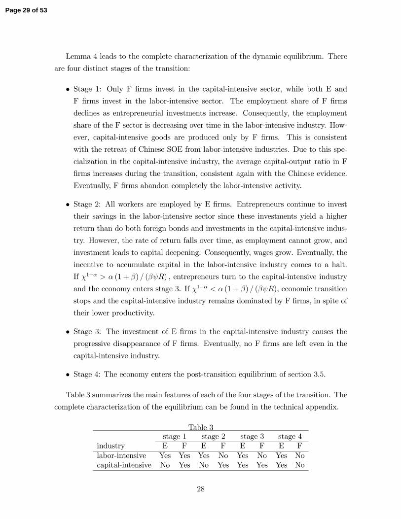
natural proxy for the di¤erent types of �rms in our theory. Figure 3 shows a measure of
pro�tability, i.e., the ratio between total pro�ts ("operation pro�ts plus subsidies plus
investment returns") and value of �xed assets net of depreciation. The gap between
DPE and SOE is about 9 percentage points per year, similar to that reported by Islam,
Dai and Sakamoto (2006).4 Similarly, Hsieh and Klenow (2007) estimate the TFP gap
(adjusted by relative prices) between DPE and SOE to be 42%.
FIGURE 3 HERE
FIGURE 4 HERE
3The disaggregation of manufacturing employment into DPE and foreign-owned enterprises is notavailable. When considering data on economy-wide employment, the employment share of DPE is about�ve times as large as that of foreign �rms in 2005, according to o¢ cial statistics.
4A concern with the o¢ cial data is that the ownership classi�cation is based on ownership at thetime of initial registration. However, many �rms subsequently have been privatized. This problem isaddressed by Dollar and Wei (2007) who use survey data on 12400 �rms, classi�ed according to theircurrent ownership. They �nd the average return to capital to be twice as high in private �rms thanin fully state-owned enterprises (see Table 6 p. 23). Interestingly, collectively owned �rms also have amuch higher productivity than SOE.
6
Page 7 of 53

Financial and contractual imperfections are central in our analysis. In a cross-country
comparative study, Allen, Qian and Qian (2005) �nd that China scores low in terms of
creditor rights, investor protection, accounting standards, non-performing loans and cor-
ruption.5 In an environment of such �nancial imperfections, Chinese �rms rely heavily
on retained earnings to �nance investments and running costs. Moreover, there is evi-
dence that credit markets discriminate against private �rms. One reason might be that
the main Chinese banks are also state owned: Boyreau-Debray andWei (2005) document
that state-owned banks tend to o¤er easier credit to SOE. As a result, SOE can �nance
a larger share of their investments through external �nancing. Figure 4 shows that SOE
�nance more than 30% through bank loans vs. less than 10% for DPE. Similarly, Dollar
andWei (2007, Table 3.1, p.21) show that private �rms have less access to bank �nancing
and rely more on retained earnings and family and/or friends to �nance investments.
One should also note that, despite the rapid growth of the Chinese stock market in
recent years, equity continues to be a signi�cant source of �nancing only for SOEs and
large semi-privatized SOEs. For instance, Gregory and Tenev (2001) document that at
the end of 1999, private �rms accounted for only 1 percent of the companies listed on
the Shanghai and Shenzhen stock exchanges. The same study reports the results of a
survey of private �rms in di¤erent Chinese provinces (including Beijing) conducted in
1999 by the World Bank, showing that about 80 percent of them regarded the lack of
access to external �nance as a most serious constraint.6 Similar conclusions are reached
by Laurenceson (2002) arguing that the importance of stock markets has been insigni�-
cant relative to the aggregate amount of savings in China, and practically irrelevant for
non-SOEs.
Another sign that DPE are more �nancially constrained is that both capital-output
and capital-labor ratios are substantially lower in DPE than in SOE. In 2006 the average
capital-output ratio in SOE was 1.75 vs. 0.67 in DPE (source: China Statistics Yearbook
2007). In the same year, the capital per worker was almost �ve times larger in SOE
5Interestingly, some reforms of the �nancial system have been undertaken, including a plan to turnthe four major state-owned commercial banks into joint-stock companies. This e¤ort involves consultingforeign advisors to improve the managerial e¢ ciency of banks (Kwan 2006). In section 4 we discuss therole of �nancial development during the economic transition.
6�(These private �rms...) relied heavily on self-�nancing for both start-up and expansion. Morethan 90 percent of their initial capital came from the principal owners, the start-up teams, and theirfamilies... In the case of post-start-up investments, the sample �rms continued to depend overwhelminglyon internal sources, with at least 62 percent of their �nancing coming from the principal owners or out ofretained earnings. Among external funding sources, informal channels, credit unions, and commercialbanks were about equally represented. Outside equity, including public equity, and public debt marketsplayed an insigni�cant role.�(Gregory and Tenev, 2001, p.1)
7
Page 8 of 53

than in DPE, although part of this di¤erence can be attributed to the higher average
educational attainment of SOE workers. This gap arises from both an intensive and an
extensive margin. First, SOE are more capital intensive within each industry, as shown
in Figure A1 in the appendix. Panels 1 and 2 show, respectively, the capital-output and
capital-labor ratio by ownership structure within three-digit manufacturing industries.
Second, DPE have taken over labor-intensive industries, while the share of SOE
remains high in capital-intensive industries. To document the retreat of SOE from labor-
intensive industries, we classify three-digit manufacturing industries by the capital-labor
ratio in US industries in 1996 (we do not classify them according to capital-labor rations
in China in order to avoid an endogeneity problem).7 We then match the industries listed
by the China Industrial Economy Statistical Yearbook (CIESY 2002, 2003 and 2004) to
the SIC codes.8 This leaves a total of 27 industries. Figure 5 plots the SOE share of
total employment across industries of di¤erent capital-intensity (average between 2001
and 2003). Clearly, SOE are signi�cantly more represented in industries that are more
capital intensive in the US. For instance, the SOE employment share in the ten most
capital-intensive industries is 57%, while in the ten least capital-intensive industries it
is 26%.
FIGURE 5 HERE
The economic transition of China has been accompanied by increasing inequality �
even within the urban sector. For instance, the Gini coe¢ cient of income grew from
0.36 in 1992 to 0.47 in 2004. Our theory suggests that this development may be due
in part to the slow growth of wages relative to entrepreneurial income. The pattern of
income inequality across regions can o¤er some insight. We classify Chinese provinces
by the percentage of employees in DPE over total employees in all industrial enterprises.
Figure 6 shows a high positive correlation between the Gini coe¢ cient at the provincial
level in 2006 and the employment share of DPE: provinces with more private �rms
have a substantially higher income dispersion. Although it does not prove any causal
relationship, this correlation is nevertheless interesting.
7The U.S. data are from NBER-CES Manufacturing Industry Database, available athttp://www.nber.org/nberces.
8Among 31 industries in CIESY, 18 of them �t industries at the SIC 2-digit level, and 9 can bematched to industries at the SIC 3-digit level. There is no match between CIESY and the SIC for theremaining 4 industries. Details are available upon request.
8
Page 9 of 53
FIGURE 6 HERE
3 Theory
In this section we develop a theory of economic transition that is consistent with the
facts documented in the previous section. A key prediction �also consistent with the
evidence from China �is that during the transition the economy experiences a growing
foreign surplus.
3.1 Environment
The model economy is populated by overlapping generations of two-period lived agents
who work in the �rst period and live o¤ savings in the second period. Preferences are
parameterized by the following time-separable logarithmic utility function
Ut = log (c1t) + � log (c2t+1) ;
where � is the discount factor. Agents have heterogeneous skills. Each cohort consists
of a measure Nt of agents with no entrepreneurial skills (workers), and a measure �Nt
of agents with entrepreneurial skills (entrepreneurs), whose skills are transmitted from
parents to children.9 The population grows at the exogenous rate �; hence, Nt+1 =
(1 + �)Nt. The rate � captures demographic trends, including migration from rural to
urban areas, assumed to be exogenous, for simplicity.10
There are two types of �rms, both requiring one manager, capital and labor as inputs.
Financially integrated (F) �rms are owned by intermediaries (see below) and operate as
standard neoclassical �rms. Entrepreneurial (E) �rms are owned by old entrepreneurs
who are residual claimants on the pro�ts and who hire their own children as managers.
Each �rm can choose between two modes of production (similar to Acemoglu et al.,
2007). Either the �rm delegates decision authority to its manager, or it retains direct
control on strategic decisions. There is a trade-o¤. On the one hand, delegation leads
to higher total factor productivity (TFP) �e.g., the manager takes decisions based on
superior information. More formally, a �rm retaining control has a TFP equal to A
while the TFP of a �rm that delegates authority is �A where � > 1: On the other
9Lower case will denote per-capita or �rm-level variables. Upper case will denote aggregate variables.10Since 1990 the average annual population growth rate in China has been 0.7% and the annual
growth of the urban-rural population ratio has been about 3.3% per year.
9
Page 10 of 53

hand, delegation raises an agency problem: unless monitored, the manager can steal the
output, and never be caught (as in Acemoglu, Aghion and Zilibotti, 2006). The key
assumption is that family-run E �rms are better at monitoring their managers (indeed,
the ability to monitor is the de�ning skill of an entrepreneur), and these can only divert
a share < 1 of output. F �rms, on the other hand, are weak at corporate governance,
and cannot e¤ectively monitor their managers: under delegation, all output would be
stolen.11
Given these assumptions, F �rms will always choose a centralized organization. More-
over, under a condition that will be spelled out below, E �rms prefer delegation. Thus,
the technology of F �rms is described by the following production function
yFt = k�Ft (AtnFt)1�� ;
while the technology of E �rms is represented by
yEt = k�Et (�AtnEt)1�� :
In both cases, k and n denote the capital and labor input, respectively, and capital is
assumed to depreciate fully after one period. In the case of centralized organization (F
�rms) the input of the manager is equivalent to that of a regular worker and is included
into nF : At is a TFP parameter that evolves according to
At+1 = (1 + z)At:
Consider, next, the savings decisions of the household sector. Young workers earn
a wage, w, and deposit their savings with a set of competitive intermediaries (banks)
paying a gross interest rate, Rd. They choose savings so as to maximize utility subject to
an intertemporal budget constraint, cw1t + cw2t+1=R
d = wt: This yields the optimal saving
swt = �= (1 + �)wt: Young entrepreneurs in E �rms earn a managerial compensation,
mt. Like the workers, they save a fraction �= (1 + �) of their earnings, and invest it
either in bank deposits or in their family business.
Banks collect savings from households and invest in domestic capital and foreign
bonds yielding a gross return R. Domestic investments can be channelled either to F
�rms or to old entrepreneurs who invest in their own business. However, contractual
imperfections plague the relationship between banks and entrepreneurs. Output and
11The assumption that the manager can steal the output unless he is monitored is a catch-all for avariety of moral hazard issues. Similar results would obtain if we assumed that there is a con�ict ofobjectives between managers and owners as in Aghion and Tirole (1997).
10
Page 11 of 53
pro�ts are partially non-veri�able, and entrepreneurs can only pledge a share � of the
second-period net pro�ts.12 In the benchmark model, we will make the simplifying
assumption that � = 0, i.e., there is no lending from banks to private entrepreneurs.
This extreme assumption will be generalized to � > 0 in section 4.1.
In a competitive equilibrium where banks invest in both foreign bonds and domestic
capital, the rate of return on domestic �rms �absent other frictions �must equal the rate
of return on foreign bonds, and both rates must equal the rate of return on deposits.13
More formally, Rd = Rl = R where Rl is the return on capital investment in domestic
�rms. Moreover, pro�t maximization implies that Rl equals the marginal product of
capital in the F sector, and that wages equal the marginal product of labor,
wt = (1� �)� �Rl
� �1��
At: (1)
Next, consider E �rms. The value of a �rm owned by an old entrepreneur who has
invested kEt is the solution to the following program:
�t (kEt) = maxmt;nEt
�(kEt)
� (�AtnEt)1�� �mt � wtnEt
(2)
subject to the incentive constraint that mt � (kEt)� (AEtnEt)
1�� ; where mt is the
payment to the manager, and arbitrage in the labor market implies that the wage is as
in (1).14 The optimal contract implies that the incentive constraint is binding:
mt = (kEt)� (�AtnEt)
1�� : (3)
Taking the First Order Condition with respect to nE and substituting in the equi-
librium wage given by (1) yields
nEt = ((1� )�)1�
� �Rl
�� 11�� kEt
�At; (4)
which in turn implies, together with (2) and (3), that the value of the �rm is
�t (kEt) = (1� )1� �
1��� RlkEt � �EkEt: (5)
12The assumption that output is not veri�able rules out the possibility that �nancially integrated�rms hire old entrepreneurs. If the entrepreneurs could commit to repay, all �rms would be run byprivate entrepreneurs.13In section 4 we assume that banks are subject to iceberg costs when turning savings into domestic
investments. In that case, Rl > R:14The managerial compensation must also exceed the workers�wage rate (mt > wt). We assume that
this participation constraint is never binding in equilibrium.In constrast, F �rms are not subject to any incentive constraint since their managers make no dis-
cretionary decisions. Thus, the managers�participation constraint is binding and they earn the samewage as ordinary workers.
11
Page 12 of 53

We introduce the following assumption:
Assumption 1 � > � ��
11�
� 11��.
Assumption 1 ensures that �E > Rl; so that (i) E �rms prefer delegation to cen-
tralization and (ii) young entrepreneurs �nd it optimal to invest in the family business.
If this assumption were not satis�ed, there would be no E �rms in equilibrium. Thus,
Assumption 1 is key to trigger economic transition.
Before discussing the equilibrium dynamics, we review the main assumptions of this
section.
3.2 Discussion
The theory describes a general growth model characterized by heterogeneous �rms that
di¤er in productivity and access to credit markets. In the application to China, the
natural empirical counterparts of E �rms and F �rms are state-owned and private en-
terprises, respectively. In our model, we do not emphasize the public ownership of less
productive �rms. However, we focus on two salient features that are related to the
ownership structure. First, due to their internal bureaucratic structure, SOE are weak
in corporate governance, and grant less autonomy and incentives to their management.
This feature is well documented. For instance, Liu and Otsuka (2004) documents that
pro�t-linked managerial compensation schemes are very rare in a sample of SOE, and in
contrast are ten to twenty times more prevalent in a sample of Township and Village En-
terprises. The rigidity of the SOE structure is emphasized by Chang and Wong (2004).
Second, thanks to connections to state-owned banks they enjoy better access to borrow-
ing (see the motivating evidence discussed above). In describing F �rms as competitive,
we abstract from other institutional features, such as market power or distortions in
the objectives pursued by �rms and their managers, that may be important in Chinese
SOE. We do so partly for tractability. We note, however, that SOE in China have been
subject to an increased competitive pressure that has led many of them to be closed or
privatized and forced to restructure. Therefore, we believe the abstraction of competitive
pro�t-maximizing �rms to be fruitful in order to focus on the two distortions discussed
above. Likewise, again for simplicity, we model the labor market as competitive and
frictionless. While the Chinese labor market is characterized by important frictions (for
example, barriers to geographical mobility) we do not think that including such frictions
would change any of the qualitative predictions of the theory, although it would a¤ect
the speed of reallocation.
12
Page 13 of 53

The assumption that private �rms are less �nancially integrated is also well rooted
in the empirical evidence discussed in section 2, showing that Chinese private �rms rely
heavily on self-�nancing, and receive only limited funding from banks and insigni�cant
equity funding. The assumption that monitoring is easier within �exible organizations
�and most notably in family �rms �seems natural. In the model, we do not emphasize
inter-family altruistic links: parents transmit genetically entrepreneurial skills to their
children, but also must provide them with incentives to avoid opportunistic behavior.
Alternatively, we could have focused on parental altruism and assumed that incentive
problems are altogether absent in family �rms. In such an alternative model, parents
would leave voluntary bequests to their children, who in turn would invest in the family
�rm. In the technical appendix we develop a model with warm-glow bequests, and show
that the main implications of the theory are robust. One advantage of the speci�cation
chosen in the previous section is that it does not hinge on family ties. For instance,
we could dispense of the assumption that young managers and old entrepreneurs in E
�rms are members of the same family, and assume instead that entrepreneurial skills
� i.e., the ability to monitor �can be learned through the experience of working as a
manager with delegated authority. The results would be identical to those of our model.
Therefore, the model captures general features of private credit-constrained �rms beyond
the convenient abstraction of the family �rm.
The feature that is essential for our mechanism to work is that �nancial and contrac-
tual frictions must obstruct the �ow of capital towards high-productivity entrepreneurial
�rms. If the entrepreneurs could borrow external funds without impediments, the tran-
sition would occur instantaneously and only the more e¢ cient E �rms would survive in
equilibrium. As we will see, the fact that entrepreneurs must rely �partially or totally
�on their own savings generates a smooth transition.
3.3 Equilibrium during transition
In this section, we characterize the equilibrium dynamics during a transition in which
there is positive employment in both sectors. We start by showing that E �rms choose
in equilibrium a lower capital-output ratio than do F �rms. To this aim, denote by
�J � kJ= (AJnJ) the capital per e¤ective unit of labor. We drop time subscripts when
this causes no confusion. As discussed above, in a competitive equilibrium, the borrowing
rate, Rl, pins down the marginal product of capital in the F sector. Thus, Rl = ����1F ,
13
Page 14 of 53

implying
�F =� �Rl
� 11��
: (6)
Since �F is constant, the equilibrium wage in (1) grows at the rate of technical change,
z; as long as employment in the F sector is positive. This is a standard feature of
neoclassical open-economy growth models. Equation (4) then implies immediately that
�E = �F ((1� )�)�1� ; (7)
where �E < �F as long as Assumption 1 holds. The following Lemma is then easily
established.
Lemma 1 Let Assumption 1 hold, i.e., � > �: Then, E �rms have a lower capital-
output ratio and a lower capital-labor ratio than do F �rms.
Intuitively, �nancially constrained �rms have a comparative disadvantage in using
capital � manifested in the higher return on capital � and therefore choose a lower
capital-labor ratio.
Consider, next, the transitional dynamics of capital and labor. The key properties of
the model that determine the equilibrium dynamics are that (i)KEt and At are predeter-
mined (whereas KFt is not a state variable, and is determined so as to equate the return
on investments in the F sector to the international bond rate), (ii) capital per e¤ective
unit of labor, �E and �F ; are constant in each sector, and (iii) entrepreneurial saving at
t (hence, KEt+1) is linear in KEt: These three properties imply that employment, capital
and output in the entrepreneurial sector grow at a constant rate during transition, as is
stated formally in the following Lemma.
Lemma 2 During transition, given KEt and At, the equilibrium dynamics of capital
and employment in the entrepreneurial sector are given by:
KEt+1
KEt
=�
1 + � ((1� )�)
1���Rl
�� 1 + KE
; (8)
and NEt+1=NEt =�1 + KE
�= (1 + z) � 1 + �E: The employment share of the entrepre-
neurial sector grows over time if and only if �E > �, or, equivalently
� >1
1�
�1 + �
�
(1 + z) (1 + �)
�
Rl
� �1��
: (A2)
14
Page 15 of 53
The fact that young entrepreneurs earn a constant share of E-�rms�pro�ts is a key
driving force of the transition. To illustrate this point, suppose that z = 0: In this
case the workers�wage remains constant during the transition. However, the managerial
rents, mt; still grow in proportion to the output of the E sector. The growing earning
inequality between workers and entrepreneurs is key for the transition to occur, since
(i) the investments of E �rms are �nanced by entrepreneurial savings, and (ii) constant
wages avoid a falling return to investments. If young entrepreneurs were to earn no
rents and to receive the workers�wage, investments in the E sector would not grow over
time. As one can see from (8), the growth rate is hump-shaped in : If entrepreneurial
rents are small (low ), young entrepreneurs are poor, and there are low investments.
However, if is too large, the pro�tability and growth of E-sector �rms (�E) fall.
Note that both Assumption 1 and condition A2 require the TFP gap, �; to be large.
Hence, generically, only one of them will be binding. Interestingly, the theory can predict
failed take-o¤s. For instance, suppose that the saving rate, �= (1 + �), unexpectedly
falls. Then, it is possible that investments in the E sector continue to be positive (i.e.,
Assumption 1 continues to hold) but the employment share of the E sector shrinks (i.e.,
condition A2 ceases to be satis�ed).
The equilibrium dynamics of capital, employment and output of the F sector are
characterized residually by the condition that KFt = �FAt (Nt �NEt), namely the F
sector hires all workers not employed in the E sector, and KF adjusts so as to attain the
optimal capital-labor ratio. Standard algebra shows that, as long as the employment
share in the E sector increases, the growth rateKF declines over time.15 Capital accumu-
lation in the F sector is hump-shaped during the transition. Initially, when employment
in the E sector is small, KF grows at a positive rate. However, as the transition proceeds,
its growth rate declines and eventually turns negative.
Finally, standard algebra shows that GDP per worker is given by
YtNt
=YFt + YEt
Nt
= ��F
�1 +
1�
NEt
Nt
�At: (9)
15More formally,
KFt+1
KFt=AFt+1AFt
NFt+1NFt
= (1 + z) (1 + �)1� NE0
N0
�1+�E1+�
�t+11� NE0
N0
�1+�E1+�
�t � 1 + KF t:
where ddt
�1 + KF ;t
�= (1 + z) NE0
N0
�1+�E1+�
�t �ln 1+�E1+�
����E�
1�( 1+�E1+� )t�2 < 0 as long as NE=N grows.
15
Page 16 of 53

The growth rate of GDP per worker accelerates during transition as long as condition
(A2) is satis�ed, re�ecting the resource reallocation towards more e¢ cient �rms. Under
the same condition, the average rate of return on capital in the economy increases
during the transition, even though the rates of return on capital in E �rms and F �rms
are constant. Intuitively, this re�ects the increasing share of the capital stock yielding
the high return �E.16
Figure 7 illustrates the transitional dynamics of employment, wage, output and av-
erage rate of return in our economy when Assumption 1 and condition A2 hold. In the
�gure, the transition ends in period T, when all workers are employed in the E sector.
During the transition, the employment share of the E sector, the average rate of return
and output per e¤ective units of labor grow, whereas wages per e¤ective units remain
constant.
FIGURE 7 HERE
3.4 Foreign Balance, Savings, and Investments
In this section, we derive the implications of the model for foreign balance, saving and
investment rate. We start from the foreign balance, which is the main focal point of our
theory. Consider the banks�balance sheet:
KFt +Bt =�
1 + �wt�1Nt�1: (10)
The left-hand side are the banks�assets (i.e., F-sector investments, KFt; plus foreign
bonds, Bt), while the right-hand side describes their liabilities (deposits). The analysis
of the previous section leads to the following Lemma.
Lemma 3 The country�s foreign balance is given by
Bt =
��
1 + �
(1� �)���1F
(1 + z) (1 + �)� 1 + NEt
Nt
��FAtNt: (11)
16More formally, the average rate of return is
�t =�EKE;t + �FKF;t
KE;t +KF;t=
Rl
1��1� � ((1� )�)�
1�
�NEt
Nt
;
which is increasing as long as NEt=Nt increases.
16
Page 17 of 53

As long as the employment share of the E sector (NEt=Nt) increases during the tran-
sition, the country�s foreign asset position increases, at least, for su¢ ciently large t.17
When the transition is completed (say, at time T), all workers are employed in E �rms
(NET=NT = 1), and the net foreign position becomesBT = (�= (1 + �)) (1� �)��FATNT >
0:
The intuition for the growing foreign surplus despite rapid economic growth is that
as employment is reallocated towards the more productive E �rms, investment in the
�nancial integrated sector shrinks. Hence, the demand for domestic borrowing falls and
banks must shift their portfolio towards foreign bonds. Although there is a potentially
increasing demand of borrowing from the E sector, this cannot be satis�ed due to the
�nancial frictions. Interestingly, the growth rate of the foreign surplus can exceed that
of GDP, resulting in a growing Bt=Yt ratio.18
Figure 8 illustrates the evolution of the foreign balance-GDP ratio during transition
through a simulated example.
FIGURE 8 HERE
During the transition, the gross saving rate, St=Yt (where St = (�= (1 + �)) (wtNt + �mt)),
is increasing, whereas the gross investment rate, It=Yt (where It = KEt+1 + KFt+1), is
decreasing. Both forces contribute to the growing foreign trade surplus during the tran-
sition. Consider, �rst, why the saving rate grows. Workers employed in the F sector earn
a constant share, 1� �, of output in that sector, and save a fraction �= (1 + �) of this.
In contrast, workers employed in the E sector save a fraction (�= (1 + �)) (1� �) (1� )
of output in that sector. In addition, young entrepreneurs save a share (�= (1 + �)) .
Thus, the saving rate of the E-sector equals (�= (1 + �)) (1� �+ � ) which exceeds the
corresponding rate in the F sector. Since the E sector expands over time, the average na-
tional saving rate is increasing, due to a composition e¤ect. Next, consider investments.
17When t is small, so that NEt=Nt is small, the right-hand side term in parenthesis can be negative.Thus, initially Bt may fall. However, Bt= (AtNt) is non-decreasing.18Bt=Yt grows during transition as long as is not too large. More formally,
BtYt=
�1+�
(1��)���1F
(1+z)(1+�) � 1 +NEt
Nt
1 + 1�
NEt
Nt
�1��F
which is increasing withNEt=Nt provided that <�1+��
(1+z)(1+�)1��
�Rl
�: The set of parameters satisfying
this condition together with assumption 1 and condition (A2) is non-empty.
17
Page 18 of 53

Recall that investments at t equal capital at t+1, and consider for simplicity the case of
z = � = 0. Then, every worker who is shifted from the F to the E sector works with less
capital. Therefore, the total domestic investment falls during the transition. Even with
positive technical change and population growth, the investment rate would fall over
time. It is important to note that the prediction of a growing foreign surplus does not
hinge on a falling investment rate. In the next section, we show that augmenting our
model with improvements in the �nancial sector can yield both increasing investment
rates and a growing foreign surplus during transition.
The following proposition summarizes the main results so far.
Proposition 1 Suppose Assumption 1 holds. During a transition, the equilibrium em-
ployment in the two sectors is given by NEt = KEt=�At�F (1� )�
1� ��
1���
�and NFt =
Nt�NEt, where �F is given by (6), and KEt and At are predetermined at t. The rate of
return to capital is constant over time in both sectors, and higher in the E than in the
F sector: �F = Rl and �E = (1� )1� �
1��� Rl: The capital and employment growth of
the E sector are given by (8). If condition A2 holds, then the employment share of the
E sector grows over time. The stock of foreign assets, given by (11), is growing.
3.5 Post-transition Equilibrium
Once the transition is completed at period T all workers are employed in E �rms,
NEt = Nt for t > T . Moreover, the aggregate capital stock is given by KEt+1 =
(�= (1 + �)) mt, which implies standard neoclassical dynamics of capital per e¢ ciency
units;
�Et+1 =�
1 + �
(1 + z) (1 + �)(�Et)
� :
Thus, there is capital deepening over time until the capital per e¢ ciency unit converges.
Consequently, wage growth will increase, and output and net foreign surplus will increase
until the capital deepening is completed. However, the rate of return on capital will
decrease. Figures 7 and 8 illustrate the post-transition dynamics of the main variables.
3.6 Discussion
The theory �ts some salient qualitative features of the recent Chinese growth experience
discussed in section 2. First, in spite of the high investments and growth of industrial
production the corporate rate of return does not fall. Second, E �rms �similarly to DPE
in China �have a higher TFP and less access to external �nancing. This induces a lower
18
Page 19 of 53
capital intensity in E �rms than in F �rms (Lemma 1) �again in line with the empirical
evidence. Moreover the rate of return on capital is higher in E �rms than in F �rms, as
in the data DPE are more pro�table than SOE. Third, the transition is characterized
by factor reallocation from �nancially integrated �rms to entrepreneurial �rms �similar
to the reallocation from SOE to DPE in the data. Fourth, such reallocation leads to an
external imbalance �as in the data the economy runs a sustained trade surplus. Finally,
the model predicts a growing inequality between wages and entrepreneurial earnings.
The most problematic prediction is that of a falling investment rate during the tran-
sition. As explained above, the mechanism behind this prediction is very di¤erent from
that of a standard neoclassical growth model. There, the investment rate falls due to
capital deepening and decreasing returns. In contrast, in our model, the investment
rate falls due to a composition e¤ect: �nancially constrained �rms - which have a lower
capital-output ratio - expand, while �nancially unconstrained �rms contract. However,
in the data there is no evidence of a falling investment rate: Bai, Hsieh and Qiang (2006)
document that the aggregate investment-GDP ratio has been U-shaped since 1992, with
a trough in 1997. In 2006, the investment rate was a staggering 52%!
One way to reconcile our theory with the data is to introduce a mechanism generating
capital deepening within each sector. This would be consistent with the evidence that
both private and state-owned �rms in China have increased their capital-output ratio
over time (whereas capital-output ratios are constant within each sector in our model).
One simple mechanism delivering capital deepening is a reduction of �nancial frictions
during the transition. We turn to �nancial development in the next section.
4 Financial development
There have been some attempts to improve the Chinese �nancial system during recent
years. For instance, the lending market has been deregulated, allowing for both more
competition and more �exibility in pricing of loans.19 This has brought an increase in
the e¢ ciency of the banking system, witnessed for instance by a sharp reduction in the
ratio of non-performing loans.20 To incorporate �nancial development into the theory,
19Before 1996, banks had to lend at the o¢ cial lending rate. In 1996, a reform allowed them to setthe rate between 0.9 and 1.1 times the o¢ cial rate. The upper limit gradually increased to 1.3 timesfor small and medium enterprises in the late 1990s and was eventually removed completely in 2004(see Ouanes, 2006). The increase in competition is also witnessed by the loan share of the four majorstate-owned banks falling from 61% in 1999 to 53% in 2004 and by the growing equity market.20In state-owned banks, the non-performing loan ratio has fallen from 26% in 2002 to 10% in 2005.
Although part of this improvement can be attributed to a government bailout, this ratio for new loans
19
Page 20 of 53

we introduce intermediation costs and let them vary over time. In particular, banks
incur an iceberg cost, �; by which for every unit of domestic investment made at t�1, �tunits get lost in real costs such as operational costs, red tape, etc. Thus, � is an inverse
measure of e¢ ciency. The equilibrium rate of return in F �rms then becomes
Rlt =
R
1� �t: (12)
Recall that a larger Rl reduces capital intensity in the F sector (see equation (6)). Since
�E = �F ((1� )�)�1� ; a high Rl also reduces capital intensity in the E sector. Consider
�nancial development in the form of a reduction of the iceberg cost. Ceteris paribus, the
fall in � leads to a reduction in Rlt; which in turn implies an increase in wages and in the
capital intensity of both sectors. Consequently, if � falls su¢ ciently fast over time, it
can o¤set the tendency of the investment rate to fall (and of the average rate of return
to increase) during the transition. In conclusion, a version of our model augmented
with the plausible assumption that the e¢ ciency of the �nancial system increases over
time can be consistent with the non-decreasing investment rate, rates of return, and
capital-output ratio observed in China.
We provide a numerical example to illustrate the possibility that, under �nancial
development, the investment rate increases and the average rate of return on capital
falls during the transition, while the implication of a growing foreign surplus remains.
To this end, we introduce �nancial development in the form of a reduction in the iceberg
cost �t such that the (annualized) rate of return in F �rms (Rl) falls gradually from 10%
to 6.5% between the start and the endpoint of the transition, assuming one period to
be 30 years. We set � = 0:5 to match the initial labor share and set the annualized
population growth rate to 1%. The growth rate of productivity is 5% per year.21 In
addition, we set � = 1; = 0:4, and � = 3:7: This corresponds to an economy where the
aggregate saving rate is initially 25% and goes up to 35% at the end of the transition.
Moreover, the annualized rate of return to E �rms falls from 11% to 7.5%, staying always
1% above that of F �rms.22
after 2000 is reported to have fallen drastically compared with older loans (see Ouanes, 2006).21In our simple model there is no scope for improvements in the quality of the labor force, which
has been an important driving force of growth in China. Thus, z captures both technical progressand human capital accumulation. The value of z is not essential, and qualitatively and quantitativelysimilar transitions as in Figure 9 can be obtained from a large range of values for z.22The simplifying assumption that all agents have the same discount factor imposes strong constraints
on the set of admissible parameters. Conceptually, the growth of B=Y and I=Y are governed by twodi¤erent forces: low initial B=Y (and subsequently growing B=Y ) require that the workers� savingrate be not too high. Instead, a growing I=Y requires that the �nancial development (i.e., the fall in
20
Page 21 of 53

FIGURE 9 HERE
Figure 9 plots the outcomes of this economy (dotted line) compared to outcomes
in the absence of �nancial development (solid line), where the only di¤erence is the
exogenous evolution of iceberg costs re�ected in the rate of return to F �rms, plotted
in Panel 1. To facilitate comparison, both economies start out with the same initial
entrepreneurial capital. Transition to full employment in the E sector is completed at
time T2 (T1) in the economy with (without) �nancial development. A lower cost of
capital implies that F �rms increase their capital intensity which, in turn, implies that
the wage per e¢ ciency units is increasing with �nancial development instead of being
stagnant as in the case without �nancial development (see equation (1) and Panel 2 of
Figure 9). An increasing wage implies capital deepening also in the E sector, even though
E �rms cannot borrow. Intuitively, the transition takes longer when there is �nancial
development because an increasing share of the entrepreneurial savings must be devoted
to increase capital intensity and, hence, labor productivity in the E sector. Consequently,
the capital-output ratio increases in both sectors, implying that the rate of return falls
in both sectors. This, in turn, implies a an increasing aggregate capital-output ratio
(from 0.86 to 1.01 during the transition), and a falling average rate of return (Panel 3).
The increased capital deepening also ensure a higher growth rate of aggregate output in
the �rst phase of the transition (Panel 4). Due to the increased capital intensity in both
sectors, the investment rate actually increases during the transition in this numerical
example (Panel 5). Increased investment mitigates the foreign surplus accumulation.
However, the key prediction of a growing foreign surplus is maintained in this example
(Panel 6).23
Rlt) be su¢ ciently large. However, a low Rlt would violate condition A2 and terminate the transitionprematurely unless � is su¢ ciently high or the entrepreneurs have su¢ ciently high saving rates tosustain the growth of the E sector. Hence, the need for large � and hinge on the stark assumption ofequal discount factors.Alternatively, if we were to assume, realistically, that entrepreneurs have a higher saving rate than
workers, the model could, for low values of and �, generate even larger increases in I=Y and B=Yduring the transition than in the economy displayed in Figure 9. This is the case if, for example, = 0:2, � = 1:8, and the workers� annualized discount factor to 0:943, maintaining � = 1 for theentrepreneurs. See the technical appendix for details.23When expressed as a fraction of GDP, net foreign assets increase from 43% to 77%. In contrast, in
the data the foreign asset-GDP ratio of China increased from 5% to over 43% between 1992 and 2008.As discussed above, it is di¢ cult to match the low initial ratio if we maintain a common discount rate.However, it is easy to replicate quantitatively the empirical observation if we assume that workers havea lower discount factor, equal to an annualized 0.96% rate.
21
Page 22 of 53

4.1 Bank Lending to the Entrepreneurial Sector
A limitation of the analysis so far is that �nancial development a¤ects directly only
�nancially unconstrained F �rms. Capital deepening also occurs in the E sector, but
this is due to a general equilibrium e¤ect through wages. In this section, we generalize
the model by allowing E �rms to �nance part of their investments through bank loans.
The possibility to partially leverage investments grants entrepreneurs a higher return on
their savings �they borrow at the rate Rl and earn a rate of return equal to �E > Rl.
We assume that entrepreneurs can borrow, but can only pledge a share � > 0 of
the second-period net pro�ts. The fraction 1 � � is not veri�able. The principal-agent
problem, (2), is unchanged, and both �t (kEt) and �E continue to be de�ned by (5).
However, the �rm size is, now, kEt+1 = sEt +lEt ; where s
E is the saving of the entrepreneur,
and lE is the bank loan. The incentive-compatibility constraint of the entrepreneur
implies that
RllE � ��E�sE + lE
�; (13)
where Rl = R= (1� �) denotes the borrowing rate. Note that a reduction in � will now
lower the borrowing cost for both sectors. In equilibrium, the incentive-compatibility
constraint binds. Thus, the share of E-sector investments �nanced through bank loans
is:lE
lE + sE=��ERl
: (14)
The entrepreneur�s investment problem can be expressed as
maxlE ;sE log�m� sE
�+ � log
��E�lE + sE
��RllE
�, subject to (14). Using the con-
straint to substitute away lE; the program simpli�es to
maxsE
log�m� sE
�+ � log
�(1� �) �ER
l
Rl � ��EsE�:
The saving decision is not a¤ected by the availability of bank loans, due to standard
properties of the logarithmic utility. However, the E-sector will grow faster, as bank
�nancing now works as an accelerator. Savings and external �nancing determine capital
accumulation in the E sector:
kEt+1 = lEt + sEt =�
1 + �
((1� )�)1���
1� � (1� )1� �
1���
R
(1� �)�kEt
where we have substituted Rl; m and �E by their equilibrium expressions. A number of
insights emerge:
22
Page 23 of 53

1. Financial development in the form of an increase in �, i.e., better credit market
access for entrepreneurs unambiguously speeds up transition. However, it a¤ects
neither the capital intensity (�E) nor the wage rate during the transition. The
reason is that the economy-wide wage rate is not a¤ected by � as long as F �rms
remain in operation.
2. Financial development in the form of a reduction of �, i.e., lower iceberg inter-
mediation cost in both sectors, unambiguously slows down transition. Moreover,
it increases the capital intensity (�E) and the wage rate. This result depends on
the logarithmic speci�cation. In particular, a lower � increases the rate of return
on entrepreneurial investments, but this does not a¤ect their savings. In addition,
the share of bank loans is independent of �: This can be seen by noting that both
Rl and �E depend on � but their ratio does not. Hence, the right-hand side of
equation (14) is invariant to �:
3. As long as �nancial development takes the form of a simultaneous increase in �
and reduction in �, the model predicts capital deepening within each sector, and
an ambiguous e¤ect on the speed of transition.
4. The foreign asset position is determined by the condition
KFt +��ERl
KEt +Bt =�
1 + �wt�1Nt�1:
Now, the e¤ect of growth on the foreign asset position is ambiguous: for low �,
the economy still accumulates a foreign surplus, while the opposite can occur if �
is large. Financial development in the form of an increase in � thus can revert the
growth in the foreign surplus.
5 Extensions and Empirical Analysis
In this section we extend the model and derive some auxiliary testable implications of
the theory. We consider two extensions. The �rst introduces region-speci�c shocks to
saving rates. A key feature of our model is that investments in E �rms are determined
by entrepreneurial savings, whereas F-sector investments are detached from domestic
savings. Whenever E �rms have a large (small) share of employment, we expect �uctu-
ations in local savings to be highly (little) correlated with �uctuations in investments �
since entrepreneurial savings is a large (small) share of local savings in this case. We test
23
Page 24 of 53

this prediction by looking at the properties of the time-series correlation between sav-
ings and investments across regions with di¤erent shares of employment in E �rms. The
second extension introduces multiple industries with di¤erent capital intensities (i.e.,
di¤erent ��s). This generates endogenous specialization of E and F �rms in more or less
capital-intensive industries, yielding testable predications about the timing of expansion
of private �rms across industries.
5.1 Savings and Investments across Regions
In this section we extend the theory to a two-region economy, region A and region B. We
assume that E �rms are located in the region where the respective entrepreneurs live,
whereas there is no restriction on capital mobility in the F sector.24 The entrepreneurial
capital stock can therefore di¤er across the two regions. This feature can be motivated
by di¤erences in local institutions a¤ecting the pro�tability of entrepreneurial activity.
To make the comparison stark, suppose that Assumption 1 holds in region A, but not
in region B. Hence, all agents in region B invest their savings in bank deposits.
Our main focus is on the cross-region correlation between savings and investments.
To this aim, we assume saving rates to be subject to region-speci�c shocks, captured by
i.i.d. stochastic �uctuations in the discount factors �rt; where r 2 fA;Bg. Under thisassumption, the theory predicts a positive time-series correlation between savings and
investments in region A, and no correlation in region B. The reason is that in region A
entrepreneurial investments are constrained by entrepreneurial savings. In contrast, in
region B investments are independent of local savings, like in an open-economy growth
model. The same argument generalize to economies with many regions: the time-series
correlation between investments and savings should be increasing with the employment
share of the E sector.25
We test this implication using a dataset covering all Chinese provinces for which
o¢ cial data have been published by the National Bureau of Statistics since 2001. This
yields a panel of 31 provinces with observations from 2001 to 2006.26 The share of the E
24The extent of labor mobility does not a¤ect the main result in this section, but only the speed oftransition in each region and in the economy as a whole.25The assumption that regions di¤er in the pro�tability of entrepreneurial activity is made for sim-
plicity. The same results would obtain if we assumed that cross-regional di¤erences in the share of E�rms are driven by di¤erent histories of realizations of ��s.26A list of these regions and summary statistics is available upon request. The employment statistics
for 2001, 2002, 2003 and 2005 are from China Industrial Economy Statistical Yearbook (various issues).The China Statistical Yearbook (2007) provides data for 2006. Annual data for investment, saving andGDP are all from China Statistical Yearbook (2002 to 2007).
24
Page 25 of 53

sector is measured by the ratio of employment in domestic private industrial enterprises
to total industrial employment in a province. Regional investment is total investment in
�xed assets in each province, and regional saving is provincial GDP minus private and
government consumption expenditures. Both investments and savings are expressed as
ratios of provincial GDP.
TABLE 1 HERE
We �rst split the sample into terciles according to the employment shares of DPE in
2001. Then, we estimate the regression
(I=Y )rt = at + ar + b � (S=Y )rt + urt; (15)
within each tercile, where where I=Y is the investment rate, S=Y is the savings rate,
and ar and at are province and year dummies, respectively. The theory predicts that
the estimated coe¢ cient b should be lowest in the bottom tercile, and highest in the
top tercile. This prediction is borne out in the data. Consider Table 1. We report
three speci�cations, where the �rst does not include time dummies, the second is the
speci�cation (15), and the third controls, in addition, for GDP per capita. In all cases,
the estimates of b are positive and highly signi�cant for the �rst and second tercile, and
insigni�cant for the third tercile. Moreover, the coe¢ cient b declines monotonically from
the lower to the higher tercile, in accordance with our theory.27
Next, we consider the entire sample (i.e., not split into terciles) and run the following
regression:
(I=Y )rt = ar + at + b1 �EMPLPRIVrt + b2 � (S=Y )rt + b3 ��(S=Y )rt � EMPLPRIVrt
�+ "rt;
27We also calculated the time-series correlation between savings and investment rates individually foreach region:
CORRr (S; INV ) =1
5
2006Xt=2001
��INVrt � INVr
� �Srt � Sr
��vuut 2006Xt=2001
�INVrt � INVr
�2vuut 2006Xt=2001
�Srt � Sr
�2where Sr and INVr are the average savings and investments in region r between 2001 and 2006. Then,we calculated the average of the correlation coe¢ cient within each tercile. This average correlation is0.74 in the top tercile (s.d. 0.31), 0.68 in the second tercile (s.d. 0.39) and 0.52 in the lowest tercile(s.d. 0.43).
25
Page 26 of 53

where EMPLPRIVrt is the share of employment in the private sector.28 Our theory
predicts a positive interaction coe¢ cient, b3; namely the e¤ect of savings on investments
should increase with the share of private �rms. The results are shown in Table 2.
Column 1 shows that the interaction coe¢ cient is positive and statistically signi�cant at
the 10% level. When we control for GDP per capita in the initial period, the interaction
coe¢ cient triples and becomes signi�cant at the 1% level (b3 is positive and signi�cant
even when time dummies are omitted).
TABLE 2 HERE
5.2 Capital- and Labor-Intensive Industries
An important feature of the Chinese transition is that the share of SOEs has declined
dramatically in labor-intensive industries, while it is still high in capital-intensive indus-
tries (see Section 2). The retreat from labor-intensive industries has further widened the
gap between the capital-output ratio of SOEs and that of private �rms since the mid
1990s (see Dekle and Vandenbroucke, 2006). Previous studies have attributed this phe-
nomenon to a strategic policy of retaining state control over large SOE and privatizing
small SOE in the late 1990s.29 Our theory provides an alternative explanation based on
�nancial frictions. To this end we extend our model to a two-sector environment. For
simplicity, we assume � = � = 0:
The �nal good, Yt; is assumed to be a CES aggregate of two intermediate goods:
Yt =�'�Y kt
���1� +
�Y lt
���1�
� ���1
: (16)
The superscripts k and l stand for capital- and labor-intensive intermediate goods, re-
spectively, and ' > 0 is a parameter. Both goods can be produced either by E or F
�rms, with the following technologies:
ylJ =�AlJ�1�� �
klJ�� �
nlJ�1��
; (17)
28Interestingly, the regional growth rate is positively correlated with EMPLPRIVrt even after con-trolling for the investment rate. This is consistent with the prediction of our theory that sectoralreallocation accelerates during the transition, see Figure 7. Results are available upon request.29The so-called policy of "grasping the large and releasing the small ones" meant to abandon control
of small SOE and support only a few large SOE in so-called "national crucial industries". The statedobjective of this policy would be to help large SOE be competitive internationally like keiretsu in Japanor chaebol in Korea. Movshuk (2004) provides a case study on the iron and steel industry.
26
Page 27 of 53
and
ykJ =�AkJ�1��
kkJ ; (18)
where J 2 fE;Fg. The production technology for the labor-intensive good is identicalto that of the benchmark model. The assumption that the capital-intensive good is
produced without labor is for convenience. We assume the same TFP gap between E
and F �rms in the two industries. More formally, � � AkEt=AkFt = AlEt=A
lF t. Note that
we raise both AkJ and AlJ to the power of 1�� to ensure that the technological advantage
of E �rms is the same in both sectors. Both �nal- and intermediate-good production
takes place under perfect competition. Assumption 1 and condition A2 are assumed to
hold.
We set the �nal good to be the numeràire. Pro�t maximization of �nal producers
subject to (16) yields:Y k
Y l=
�'P l
P k
��: (19)
The standard price aggregation holds:�'��P k�1��
+�P l�1��� 1
1��= 1: (20)
When F �rms are active in the production of the labor-intensive good, they behave as
in the benchmark model of section 3. In particular, the following analogues of equations
(1) and (6) hold:
wt = P lt (1� �)AlF t
��lF t��; (21)
�lF t =
�P lt�
R
� 11��
: (22)
In addition, when F �rms are active in the production of the capital-intensive good,
perfect competition pins down its price level:
P kt
�AkFt�1��
= R: (23)
Given these equilibrium conditions, we can determine the return for E �rms to invest
in each industry. The following Lemma characterize the patterns of specialization of F
and E �rms. Recall that KEt is predetermined by the entrepreneurial savings.
Lemma 4 (i) If, at time t, K lF t > 0 and Kk
Ft > 0; then �lEt > �kEt; implying that
K lEt = KEt and Kk
Et = 0: (ii) If, at time t, KlEt > 0 and K
kEt > 0; then R � �kFt > �lF t;
implying that K lF t = 0 and K
kFt � 0:
27
Page 28 of 53
Lemma 4 leads to the complete characterization of the dynamic equilibrium. There
are four distinct stages of the transition:
� Stage 1: Only F �rms invest in the capital-intensive sector, while both E andF �rms invest in the labor-intensive sector. The employment share of F �rms
declines as entrepreneurial investments increase. Consequently, the employment
share of the F sector is decreasing over time in the labor-intensive industry. How-
ever, capital-intensive goods are produced only by F �rms. This is consistent
with the retreat of Chinese SOE from labor-intensive industries. Due to this spe-
cialization in the capital-intensive industry, the average capital-output ratio in F
�rms increases during the transition, consistent again with the Chinese evidence.
Eventually, F �rms abandon completely the labor-intensive activity.
� Stage 2: All workers are employed by E �rms. Entrepreneurs continue to investtheir savings in the labor-intensive sector since these investments yield a higher
return than do both foreign bonds and investments in the capital-intensive indus-
try. However, the rate of return falls over time, as employment cannot grow, and
investment leads to capital deepening. Consequently, wages grow. Eventually, the
incentive to accumulate capital in the labor-intensive industry comes to a halt.
If �1�� > � (1 + �) = (� R) ; entrepreneurs turn to the capital-intensive industry
and the economy enters stage 3. If �1�� < � (1 + �) = (� R), economic transition
stops and the capital-intensive industry remains dominated by F �rms, in spite of
their lower productivity.
� Stage 3: The investment of E �rms in the capital-intensive industry causes theprogressive disappearance of F �rms. Eventually, no F �rms are left even in the
capital-intensive industry.
� Stage 4: The economy enters the post-transition equilibrium of section 3.5.
Table 3 summarizes the main features of each of the four stages of the transition. The
complete characterization of the equilibrium can be found in the technical appendix.
Table 3stage 1 stage 2 stage 3 stage 4
industry E F E F E F E Flabor-intensive Yes Yes Yes No Yes No Yes Nocapital-intensive No Yes No Yes Yes Yes Yes No
28
Page 29 of 53

6 Conclusions
In this paper, we have constructed a neoclassical model augmented with �nancial and
contractual imperfections that a¤ect asymmetrically di¤erent �rms in the economy. The
theory is consistent with a number of key facts about the recent Chinese experience, most
notably sustained high returns on investments in spite of high capital accumulation,
large productivity di¤erences across �rms, reallocation from low-productivity to high-
productivity �rms (as documented by Hsieh and Klenow 2007) and the accumulation
of a large foreign surplus. A number of simpli�cations that have been made for the
sake of tractability will be relaxed in future research. In particular, the two-period
overlapping generations model with logarithmic preferences does not speak to the high
levels of savings and investments in China. Theories of entrepreneurial savings with
�nancial constraints such as Quadrini (1999) and Di Nardi and Targetti (2006) could
add additional insights to reinforce and complement the mechanism of this paper. Also,
by assuming an exogenous rate of TFP growth, we have abstracted from investments
in technology adoption which is an important driver of China�s performance. Finally,
while this paper has emphasized qualitative insights, the analysis can be extended to a
multiperiod environment amenable to quantitative evaluation.
In spite of these limitations, we believe our theory o¤ers a useful tool for understand-
ing one of the major puzzles of the recent growth experience: how is it that China grows
at such a stellar rate while taking an increasing asset position on the rest of the world?
Some commentators have tried to explain this puzzle by attributing it to government
manipulation of the exchange rate that hold the value of the Chinese currency arti�cially
low. While it is di¢ cult to falsify theories that rely on such non-economic mechanisms,
in this paper we have provided a number of empirical observations that corroborate the
mechanism of our theory.
References
Acemoglu, Daron, Philippe Aghion and Fabrizio Zilibotti (2006), �Distance to Frontier,
Selection, and Economic Growth�, Journal of the European Economic Association
4(1), 37-74.
Acemoglu, Daron, Philippe Aghion, Claire Lelarge, John Van Reenen and Fabrizio Zili-
botti (2007), �Technology, Information and the Decentralization of the Firm�, Quar-
terly Journal of Economics, 2007, 122(4), 1759-1799.
29
Page 30 of 53

Aghion, Philippe and Jean Tirole (1997), �Real and Formal Authority in Organizations�,
Journal of Political Economy 105(1), 1-29.
Allen, Franklin, Jun Qian andMeijun Qian (2005), �Law, Finance, and Economic Growth
in China�, Journal of Financial Economics 77(1), 57 �116.
Bai, Chong-En, Chang-Tai Hsieh and Yingyi Qian (2006), �The Return to Capital in
China�, Brooking Papers on Economic Activity 2, 61�101.
Banerjee, Abhijit and Esther Du�o, (2005), �Growth Theory through the Lens of Devel-
opment Economics�in H. Chenery and T.N. Srinivasan, eds. Handbook of Develop-
ment Economics, Elsevier, Vol. 1a, 473-552.
Banister, Judith (2007), �Manufacturing in China Today: Employment and Labor Com-
pensation�, Economics Program Working Paper Series EPWP 0701, The Conference
Board.
Benjamin, Dwayne, Loren Brandt, John Giles and Sangui Wang (2008), �Income In-
equality during China�s Economic Transition,� in L. Brandt and T. Rawski, eds.,
China�s Great Economic Transformation, Cambridge University Press, 729�775.
Boyreau-Debray, Genevieve and Shang-Jin Wei (2005), �Pitfalls of a State-Dominated
Financial System: The Case of China�, NBER Working Paper 11214.
Caballero, Ricardo J., Emmanuel Farhi, Pierre-Olivier Gourinchas (2006)�An Equilib-
rium Model of "Global Imbalances" and Low Interest Rates�, NBER Working Paper
11996.
Caselli, Francesco and Wilbur John Coleman II (2002), �The U.S. Technology Frontier�,
American Economic Review 92(2), 148-152.
Chang, Eric C. and Sonia M. L. Wong (2004), �Political Control and Performance in
China�s Listed Firms, Journal of Comparative Economics 32, 617-636.
Chenery, Hollis Burnley and Moises Syrquin (1975), �Patterns of Development, 1950-
1970�, Oxford University Press for the World Bank.
Dekle, Robert and Guillaume Vandenbroucke (2006), �A Quantitative Analysis of
China�s Structural Transformation�, IEPR Working Paper No. 06.51.
30
Page 31 of 53

De Nardi, Mariacristina and Marco Cagetti (2006), �Entrepreneurship, Frictions, and
Wealth�, Journal of Political Economy 114(5), 835-870.
Dollar, David and Shang-Jin Wei (2007), �Das (Wasted) Kapital: Firm Ownership and
Investment E¢ ciency in China�, NBER Working Paper 13103.
Dooley, Michael, David Folkerts-Landau and Peter Garber (2004), �Direct Investment,
Rising Real Wages and the Absorption of Excess Labor in the Periphery�, NBER
Working Paper 10626.
Fei, John C. H. and Gustav Ranis (1961), �A Theory of Economic Development�, Amer-
ican Economic Review 51(4), 533-565.
Fei, John C. H. and Gustav Ranis (1964), �Capital-Labor Ratios in Theory and in
History: Reply�, American Economic Review 54(6), 1063-1069.
Gancia, Gino and Fabrizio Zilibotti (2001), �Technological Change and the Wealth of
Nations�, Annual Economic Review, 1, forthcoming.
Gourinchas, Pierre-Olivier and Olivier Jeanne (2007), �Capital Flows to Developing
Countries: The Allocation Puzzle�, NBER Working Paper 13602.
Gregory, Neil and Stoyan Tenev (2001), �The Financing of Private Enterprise in China�,
Finance and Development - Quarterly Magazine of the IMF, 38(1).
Hsieh, Chang-Tai and Peter J. Klenow (2007), �Misallocation and Manufacturing TFP
in China and India�, NBER Working Paper 13290.
Islam, Nazrul, Erbiao Dai and Hiroshi Sakamoto (2006), �Role of TFP in China�s
Growth�, Asian Economic Journal 20(2), 127�159.
Kraay, Aart (2000), �Household Saving in China�, World Bank Economic Review, 14(9),
545-70.
Kuijs, Louis (2005), �Investment and Saving in China�, World Bank Policy Research
Working Paper 3633.
Kuznets, Simon (1966), Modern Economic Growth: Rate, Structure and Spread, Yale
University Press, New Haven.
31
Page 32 of 53

Kwan, Chi Hung (2006), �Participation of Foreign Investors in China�s State-Owned
Commercial Banks - A win-win game�, China in Transition - Research Institute of
Economy Trade and Industry http://www.rieti.go.jp/en/china/06021501.html
Laitner, John (2000), �Structural Change and Economic Growth�, Review of Economic
Studies 67(3), 545�561.
Laurenceson, James (2002), �The Impact of Stock Markets on China�s Economic De-
velopment: Some Preliminary Assessments�, Discussion Paper no. 302, University of
Queensland.
Lewis, Arthur (1954), �Economic Development with Unlimited Supplies of Labor�,
Manchester School of Economic and Social Studies 22(2), 139-91.
Liu, Deqiang and Keijiro Otsuka (2004), �A Comparison of Management Incentives,
Abilities, and E¢ ciency between SOEs and TVEs: The Case of the Iron and Steel
Industry in China�, Economic Development and Cultural Change 52(4), 759-80.
Matsuyama, Kiminori (1992), �A Simple Model of Sectoral Adjustment�, The Review of
Economic Studies 59(2), 375-387.
Matsuyama, Kiminori (2004), �Financial Market Globalization, Symmetry-Breaking and
Endogenous Inequality of Nations�, Econometrica 72(3), 853-884.
Matsuyama, Kiminori (2005), �Credit Market Imperfections and Patterns of Interna-
tional Trade and Capital Flows�, Journal of the European Economic Association
3(2-3), 714-723.
Matsuyama, Kiminori (2007), �Ricardian Trade Theory� in L. Blume and S. Durlauf,
eds. The New Palgrave Dictionary of Economics, 2nd Edition, Macmillan, Vol. 7,
183-190.
Mendoza, Enrique G, Vincenzo Quadrini and Jose-Victor Rios-Rull (2007), �Financial In-
tegration, Financial Deepness and Global Imbalances�, NBER Working Paper 12909.
Movshuk, Oleksandr (2004), �Restructuring, Productivity and Technical E¢ ciency in
China�s Iron and Steel Industry, 1988�2000� Journal of Asian Economics, 15(1),
135-51.
32
Page 33 of 53

Ouanes, Abdessatar (2006), �Progress in China�s Banking Sector Reform: Has Bank
Behavior Changed? IMF Working Paper 06/71.
Parente, Stephen, Richard Rogerson and Randall Wright (2000), �Homework in Devel-
opment Economics: Household Production and the Wealth of Nations�, The Journal
of Political Economy 108(4), 680-687.
Quadrini, Vincenzo (1999), �The Importance of Entrepreneurship for Wealth Concen-
tration and Mobility�, Review of Income and Wealth, 45(1), 1-19.
Restuccia, Diego and Richard Rogerson (2008), �Policy Distortions and Aggregate Pro-
ductivity with Heterogeneous Plants�, Review of Economic Dynamics, 11(4), 707-20.
Takayama, Akira (1965), �On a Two-Sector Model of Economic Growth with Technolog-
ical Progress �A Comparative Statics Analysis�, The Review of Economic Studies
32(3), 251-262.
Ventura, Jaume (1997), �Growth and Interdependence�, The Quarterly Journal of Eco-
nomics 112(1), 57-84.
Wang, Yan and Yudong Yao (2001), �Sources of China�s Economic Growth, 1952-99:
Incorporating Human Capital Accumulation�,World Bank Policy Research Working
Paper 2650.
Young, Alwyn (2003), �Gold into Base Metals: Productivity Growth in the Peo-
ple�s Republic of China during the Reform Period�, Journal of Political Economy
111(6), 1220 �1261.
Zhao, Suisheng (1993), �Deng Xiaoping�s Southern Tour: Elite Politics in Post-
Tiananmen China�, Asian Survey 8(33), 739�756.
33
Page 34 of 53

0
10
20
30
40
50
60
1992 1993 1994 1995 1996 1997 1998 1999 2000 2001 2002 2003 2004 2005 2006
foreign reserves difference of total deposits and loans
Figure 1: Foreign Reserves and Di¤erences between Domestic Deposits and Loans (per-centages of GDP). Data source: Chinese Statistical Yearbook various issues.
0
10
20
30
40
50
60
70
80
90
1994 1995 1996 1997 1998 1999 2000 2001 2002 2003 2004 2005 2006
Figure 2: Private employment share in manufacturing (percentage). Private employmentincludes both non-state-owned domestic and foreign-owned enterprises. Data source:Chinese Statistical Yearbook, various issues.
34
Page 35 of 53
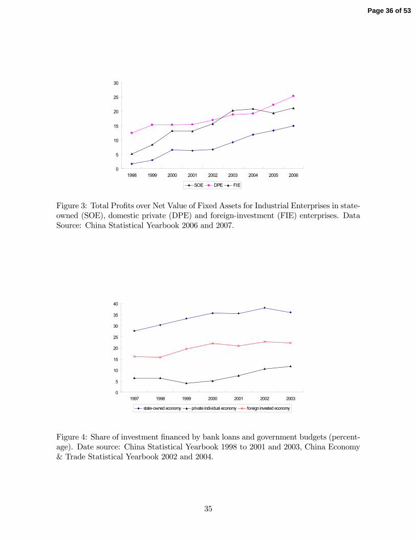
0
5
10
15
20
25
30
1998 1999 2000 2001 2002 2003 2004 2005 2006
SOE DPE FIE
Figure 3: Total Pro�ts over Net Value of Fixed Assets for Industrial Enterprises in state-owned (SOE), domestic private (DPE) and foreign-investment (FIE) enterprises. DataSource: China Statistical Yearbook 2006 and 2007.
0
5
10
15
20
25
30
35
40
1997 1998 1999 2000 2001 2002 2003
stateowned economy private individual economy foreign invested economy
Figure 4: Share of investment �nanced by bank loans and government budgets (percent-age). Date source: China Statistical Yearbook 1998 to 2001 and 2003, China Economy& Trade Statistical Yearbook 2002 and 2004.
35
Page 36 of 53
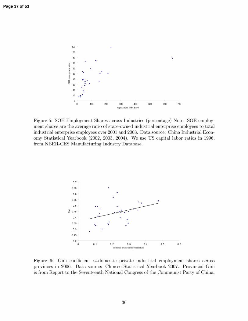
0
10
20
30
40
50
60
70
80
90
100
0 100 200 300 400 500 600 700capital labor ratios in US
SOE
empl
oym
ent s
hare
Figure 5: SOE Employment Shares across Industries (percentage) Note: SOE employ-ment shares are the average ratio of state-owned industrial enterprise employees to totalindustrial enterprise employees over 2001 and 2003. Data source: China Industrial Econ-omy Statistical Yearbook (2002, 2003, 2004). We use US capital labor ratios in 1996,from NBER-CES Manufacturing Industry Database.
0. 2
0. 25
0. 3
0. 35
0. 4
0. 45
0. 5
0. 55
0. 6
0. 65
0. 7
0 0. 1 0. 2 0. 3 0. 4 0. 5 0. 6domestic private employment share
Gin
i
Figure 6: Gini coe¢ cient vs.domestic private industrial employment shares acrossprovinces in 2006. Data source: Chinese Statistical Yearbook 2007. Provincial Giniis from Report to the Seventeenth National Congress of the Communist Party of China.
36
Page 37 of 53

T0
0.2
0.4
0.6
0.8
1
T ime
Priv
ate
empl
oym
ent
E sector share of employment
T
1.08
1.085
1.09
1.095
1.1
T ime
Rho
Annualized return on capital
Averag e returnρt
→
R eturn E firms↓
R eturn F firms↑
Averag e returnρt
→
R eturn E firms↓
R eturn F firms↑
T0.015
0.02
0.025
0.03
0.035
0.04
T ime
Wag
e ra
te p
er e
ffici
ency
uni
t
Wag e
T0.04
0.05
0.06
0.07
0.08
0.09
T ime
Out
put
Output per efficiency unit
Figure 7: Transition and post-transition dynamics.
T0.25
0.26
0.27
0.28
0.29
0.3
0.31
0.32
Time
Sav
ings
rat
e
Aggregate savings rate: S/Y
T0.2
0.4
0.6
0.8
1
1.2
1.4
1.6
Time
Fore
ign
asse
ts
Ratio of net foreign assets to GDP (annualized)
Figure 8: Saving rate and balance of payment surplus.
37
Page 38 of 53

T_1 T_2
1.07
1.08
1.09
1.1
Time
R/(1
ξ)
Annualized borrowing rate, net of iceberg cost
T_1 T_20.12
0.14
0.16
0.18
0.2
Time
Inve
stm
ent
/ GD
P
Gross Inv estment to Output Ratio
T_1 T_20.015
0.02
0.025
0.03
0.035
TimeW
age
Wage rate per ef f iciency unit
T_1 T_2
0
1
2
3
4x 10³
Time
Fore
ign
asse
ts
Foreign assets per ef f . unit
T_1 T_2
0.04
0.06
0.08
0.1
0.12
Time
YOutput per ef f iciency unit
T_1 T_2
1.08
1.09
1.1
1.11
Time
Rho
Annualized av erage return on capital
Figure 9: Transition with �nancial development.
38
Page 39 of 53
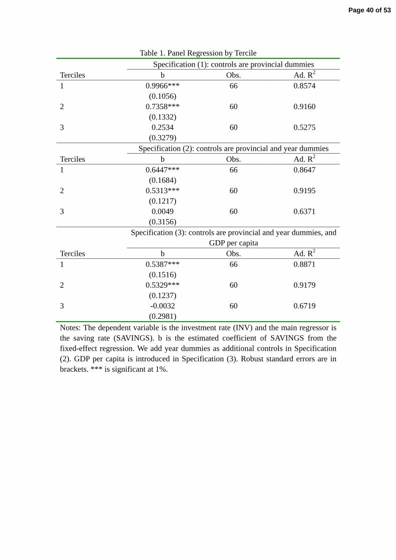
Table 1. Panel Regression by Tercile Specification (1): controls are provincial dummies Terciles b Obs. Ad. R2 1 0.9966***
(0.1056) 66 0.8574
2 0.7358*** (0.1332)
60 0.9160
3 0.2534 (0.3279)
60 0.5275
Specification (2): controls are provincial and year dummies Terciles b Obs. Ad. R2 1 0.6447***
(0.1684) 66 0.8647
2 0.5313*** (0.1217)
60 0.9195
3 0.0049 (0.3156)
60 0.6371
Specification (3): controls are provincial and year dummies, and GDP per capita
Terciles b Obs. Ad. R2 1 0.5387***
(0.1516) 66 0.8871
2 0.5329*** (0.1237)
60 0.9179
3 -0.0032 (0.2981)
60 0.6719
Notes: The dependent variable is the investment rate (INV) and the main regressor is the saving rate (SAVINGS). b is the estimated coefficient of SAVINGS from the fixed-effect regression. We add year dummies as additional controls in Specification (2). GDP per capita is introduced in Specification (3). Robust standard errors are in brackets. *** is significant at 1%.
Page 40 of 53

Table 2 Investment, Saving and Private Employment
Dep. Variable INV (1) (2) EMPLPRIV 0.0347
(0.2613) -0.0101 (0.2408)
SAVINGS*EMPLPRIV 1.2342* (0.6898)
3.6284*** (0.8697)
SAVINGS 0.3827* (0.2047)
0.5013*** (0.1723)
GDP Per Capita - -0.0124*** (0.0021)
Province Dummy Yes Yes Year Dummy Yes Yes Obs. 155 155 Ad. R2 0.7731 0.8195 Notes: The dependent variable (INV) is the investment rate defined as the ratio of total investment in fixed assets to GDP. EMPLPRIV is the employment share of domestic private industrial enterprises and the saving rate SAVINGS = (GDP-C-G)/GDP, where C and G are consumption and government consumption expenditures, respectively. The sample mean is subtracted to SAVINGS and EMPLPRIV. Robust standard errors are in brackets. ***, ** and * is significant at 1%, 5% and 10%, respectively.
Page 41 of 53

7 Appendix: Not for publication
7.1 Capital-output and capital-labor ratio by ownership struc-ture.
Figure A1 reports capital-output and capital-labor ratios by ownership structure within
three-digit manufacturing industries.
0 100 200 300 400 500 600 700 800 900
Processing of Food f rom Agricul tural Product s
Manufacture of Beverages
Manufacture of Textile
Manufacture of Leather, Fur, Feather and Related Product s
Manufacture of Furni ture
Printing,Reproduction of Recording Media
Processing of Petroleum, Coking, Processing of Nuclear Fuel
Manufacture of Medicines
Manufacture of Rubber
Manufacture of Nonmetallic Mineral Product s
Smel ting and Pressing of Nonferrous Metals
Manufacture of General Purpose Machinery
Manufact ure of T ransport Equipment
Manufacture of Communication Equipment, Computers and Ot her Electronic Equipment
Manufact ure of Art work and Other Manufacturing
FI E
DPE
SOE
0 0. 5 1 1. 5 2 2. 5 3 3. 5
Processing of Food f rom Agricul tural Product s
Manufacture of Beverages
Manufacture of Textile
Manufacture of Leather, Fur, Feather and Related Product s
Manufacture of Furni ture
Printing,Reproduction of Recording Media
Processing of Petroleum, Coking, Processing of Nuclear Fuel
Manufacture of Medicines
Manufacture of Rubber
Manufacture of Nonmetallic Mineral Product s
Smel ting and Pressing of Nonferrous Metals
Manufacture of General Purpose Machinery
Manufacture of T ransport Equipment
Manufacture of Communication Equipment, Computers and Ot her Electronic Equipment
Manufact ure of Art work and Other Manufacturing
FI E
DPE
SOE
Figure A1: Capital-Labor Ratios (upper panel, thousand yuans per worker) and
Capital-Output Ratios by Ownership and Sector in Manufacturing in 2006
(yellow=FIE, red=DPE, blue=SOE).
1
Page 42 of 53

7.2 Proofs of Lemmas
Proof of Lemma 1. That the capital-output ratio is higher in F �rms follows
immediately from the fact that �E < �F (shown in the text), since kE=yE = �1��E <
�1��F = kF=yF : Similarly, that the capital-labor ratio is higher in F �rms follows from
observing thatkFnF=kEnE
=�FA=�E�A
=
��
�
� 1���
> 1
where the inequality again follows from Assumption 1.
Proof of Lemma 2. Due to constant-return-to-scale, aggregation holds, thus we can
replace individual-�rm variables (lower case) by aggregate variables (upper case). Since
�E � KEt= (�AtNEt) is constant and NFt = Nt �NEt; then
NEt =KEt
�At�E; NFt = Nt �
KEt
�At�E; (24)
where �E is given by (7).
The saving of each young entrepreneur is given by sEt = kEt+1 = (�= (1 + �))mt: Using
(3), and aggregating over all entrepreneurs yields:
KEt+1 =�
1 + � ��E�AtNEt: (25)
Dividing both sides of (25) by KEt; and substituting �E by its equilibrium expression,
we obtain (8). That NEt+1=NEt = (KEt+1=KEt) = (1 + z) follows from (24).
The second part of the Lemma follows from the de�nitions of KEand �E; given (8).
Standard algebra shows that condition (A2) is necessary and su¢ cient for �E > �.
Proof of Lemma 3. Using equation (24), and recalling that �E and �F are constant,
we can rewrite (10) as:
Bt =
��
1 + �wt�1Nt�1 �KFt
�=
�Nt�1
Nt
�
1 + �
wt�1At
� �FNFt
Nt
�AtNt
=
�Nt�1
Nt
�
1 + �(1� �)��F
At�1At
� �F
�1� NEt
Nt
��AtNt
=
��
1 + �
(1� �)���1F
(1 + z) (1 + �)� 1 + NEt
Nt
��FAtNt;
which proves the Lemma.
2
Page 43 of 53
Proof of Lemma 4. Part (i). We start by proving that �lE = (1� )1� �
1��� R: To this
aim, observe that, since (assuming that the incentive constraint is binding)mt = P ltylEt;
then
�lt�klEt�= max
nEt
�(1� )P l
t
�klEt��(AEtnEt)
1�� � wtnEt
The �rst order condition yields:
nEt =klEtAlEt
�(1� ) (1� �)P l
tAlEt
wt
� 1�
Then, plugging (21) and (22) into the �rst order condition yields
nEt = ((1� )�)1�
�P lt�
R
�� 11�� klEt
AlEt(26)
Finally, plugging the optimal nEt into the pro�t function, and simplifying term, yields
the value of a E �rm in the labor intensive sector:
�t�klEt�= (1� ) klEt
�((1� )�)
1�
�1�� ��R
��1� (1� �)��1 ((1� )�)
1�
��R
��1klEt
= (1� )1� �
1��� RklEt � �lEk
lEt; (27)
where �lE is identical to �E in the one-sector model of section 3 (see equation (5)). This
is the rate of return for E �rms when F �rms are active in the labor-intensive industry.
Next, we show that, when F �rms are active in both industries, the return to in-
vestment in the capital-intensive sector for E �rms, �kE; is lower than �lE: When F �rms
are active in the capital-intensive industry, the value of a E �rm in the labor-intensive
sector is
�kt�kkEt�= (1� )P k
t
�AkEt
�1��kkEt
= (1� )�1��RkkEt � �kEkkEt
where we have used equation (23) to eliminate P kt : Finally, Assumption 1 ensures that
�lE > �kE (since (1� )1
1�� � > 1 , (1� )1� �
1��� > (1� )�1��). Thus, E �rms will
not invest in the capital-intensive sector. This completes the proof of part (i) of the
Lemma.
Part (ii). We prove the argument by constructing a contradiction. Suppose that,
when K lEt > 0 and Kk
Et > 0, K lF t > 0: Then, (21) and (22) hold true, and �lE =
(1� )1� �
1��� R as shown in the �rst part of the proof, see (27). Moreover, �lE = �kE =
3
Page 44 of 53

(1� )�1��R; since otherwise E �rms would not invest in both industries. Solving for
P kt yields
P kt = (1� )
1��� �
1�
R�AkFt�1�� > R�
AkFt�1��
where the inequality follows from Assumption 1, and P kt = R=
�AkFt�1��
is the condition
that guarantees that F �rms make zero pro�ts in the capital-intensive industries. Thus,
the inequality establishes that F �rms would be making positive pro�ts in the capital-
intensive sector, which is impossible in a competitive equilibrium. Thus, K lF t = 0 when
E �rms are active in both sectors. This concludes the proof of part (ii) of the Lemma.
7.3 The Model with Altruism
In this section, we discuss an alternative version of the model in which all parents have
a warm-glow bequest motive parameterized by the following function:
Ut = log (c1t) + � (log (c2t+1) + � log (at+1)) ;
where at+1 denotes the bequest. Agents choose consumption, savings and bequests to
maximize utility subject to the constraint that
c1t +c2t+1 + at+1
�= !t +
at1 + �
;
where � = Rd and ! = w for workers, whereas � = �E and ! = m for entrepreneurs.
Next, de�ne st � !t+at�c1t: The optimal savings and bequests are given by, respectively,
st =� + ��
1 + � + ��
�!t +
at1 + �
�; (28)
at+1 =�
1 + ��st: (29)
Combining these two equations yields the equilibrium law of motion for savings:
st =� + ��
1 + � + ��
�!t +
�
(1 + �) (1 + �)�st�1
�: (30)
Consider, the entrepreneurs. We assume altruism to be su¢ ciently large to make the
incentive constraint of the young entrepreneurs slack.30 Thus, the constraint (3) can be
30We assume that parents can reduce one-to-one their bequests if the children steal the �rm�s pro�t.Thus, childrent have no incentive to misbehave.
4
Page 45 of 53
ignored and the young entrepreneurs�income consists of pure bequests (more formally,
mt = 0). The value of an E �rm solves then
�t (kEt) � �EkEt = maxnEt
�(kEt)
� (�AtnEt)1�� � wtnEt
:
Taking the First Order Condition and using (1) to substitute in the equilibrium wage,
yields nEt = �1�
��=Rl
�� 11�� kEt= (�At), which in turn implies that
�t (kEt) = �1��� RlkEt � �EkEt: (31)
As long as � > 1, �E > Rd; implying that the rate of return to entrepreneurial invest-
ments exceeds the deposit rate. Thus, entrepreneurs invest their savings entirely in their
own business. Moreover, it is immediate that Lemma 1 holds true. Then, using (28)
and (29) for !t = 0 and � = �E = �1��� Rl, we conclude that young entrepreneurs save
and invest in their own business the amount
sEt =� + ��
1 + � + ��
�
(1 + �) (1 + �)�1��� RlkEt:
Aggregating over all entrepreneurs yields:
KEt+1 =� + ��
1 + � + ��
�
(1 + �) (1 + �)�1��� RlKEt: (32)
The analysis of the transition is then as in the benchmark case.
To study the external balance, consider the banks�balance sheet:
KFt +Bt = SWt�1Nt�1: (33)
where SW denotes the total savings of the workers as given by Equation (30). Using the
expression for the equilibrium wage, (1), one can rewrite the equilibrium law of motion
of SW , (30), as
sWt =� + ��
1 + � + ��
�(1� �)
� �Rl
� �1��
+�R
(1 + �) (1 + �) (1 + z)sWt�1
�: (34)
where sWt � SWt =At. As long as
� + ��
1 + � + ��
�R
(1 + �) (1 + �) (1 + z)< 1; (35)
sFt is a converging sequence. Solving the di¤erence equation in this case yields:
sFt =� + ��
1 + � + ��(1� �)
� �Rl
� �1�� 1� (�R)t
1� �R+ (�R)t sF�1;
5
Page 46 of 53

where sW�1 denotes for the initial savings of the workers and � � �+��1+�+��
�(1+�)(1+�)(1+z)
.
Note that if sW�1 is su¢ ciently low sFt is increasing along the transitional path.
Standard algebra leads then to an analogue of equation (11):
Bt =
�sWt�1
(1 + z) (1 + �)�F� 1 + NEt
Nt
��FAtNt:
As long as (i) the employment share of the E sector and (ii) the workers�savings, sW ,
increase during the transition, the country�s foreign asset position increases. Therefore,
the main results of Lemma 3 and Proposition 1 carry over to the model with warm-glow
bequests.
7.4 Post-Transition Equilibrium
The equilibrium wage, rate of return on capital, output and foreign balance are given
by:
wt = AEt (1� �) (1� ) (�E;t)�
�t = �E;t = � (1� ) (�E;t)��1
Yt = AEtNt (�E;t)�
Bt
AtNt
=�
1 + �wt
Nt
AtNt
=�
1 + �� (1� �) (1� ) (�Et)
�
Then capital in the E-sector evolves according to (25) and eventually converges to a
steady state. If (1� )� (1 + �) (1 + z) (1 + �) = (� R) > 1; then limt!1 �E > R, and
entrepreneurs never invest in bonds. Otherwise, entrepreneurs will eventually place part
of their savings in bank deposits.
7.5 Financial Development: Alternative Parameterization
In this section we describe an alternative parameterization of our economy where workers
and entrepreneurs have di¤erent savings rates. The purpose of this experiment is to
illustrate that with di¤erent savings rates the model can deliver large increases in foreign
assets and domestic investment even with quite low values for and �. In particular,
we set = 0:2 and � = 1:8 and assume that workers have an (annualized) discount
factor of 0:943, while maintaining � = 1 for entrepreneurs (where one period is set to
thirty years, as above). The initial annual return in F �rms is set to 12%, and �nancial
development �modeled as a falling �t � causes the annual return in F �rms to fall
gradually to 9.5% at the end of the transition. Finally, capital�s share is set to � = 0:5,
6
Page 47 of 53

the annual population growth rate is 1%, and the annual technical growth rate is 4%.
Under these parameters the annualized return in E �rms is always 0.5% larger than in
F �rms (so the annualized return in E �rms start out at 12.5% and fall to 10% at the
end of the transition). Moreover, Assumption A1 and condition A2 are satis�ed.
The dynamics of the economy is displayed in �gures A2 and A3. The investment rate
grows (monotonically) by more than one third during the transition (Panel 5 of Figure
A2).The initial stock of net foreign assets is zero and grows to 40% of GDP at the end
of the transition (Figure A3 and Panel 5 of Figure A2).
T_1 T_2
1.1
1.11
1.12
T ime
R/(1
ξ)
Annualized borrowing rate, net of iceberg cost
T_1 T_20.06
0.07
0.08
0.09
0.1
T ime
Inve
stm
ent /
GD
P
Gross Investment to Output Ratio
T_1 T_20.008
0.01
0.012
0.014
0.016
T imeW
age
Wage rate per effic iency unit
T_1 T_2
0
2
4
6x 10 4
T ime
Fore
ign
asse
ts
Foreign assets per eff. unit
T_1 T_2
0.02
0.03
0.04
T ime
YOutput per effic iency unit
T_1 T_21.1
1.11
1.12
T ime
Rho
Annualized average return on capital
Figure A2
7
Page 48 of 53

T_1 T_2
0
0.05
0.1
0.15
0.2
0.25
0.3
0.35
0.4
T ime
Fore
ign
asse
ts
Ratio of net foreign assets to GDP
Figure A3
7.6 Equilibrium in Section 5.2
In this appendix, we provide a formal characterization of the equilibrium in the two-
sector economy of Section 5.2. The equilibrium entails are four stages, described in the
text. For notational convenience, we let AkJt = AlJt = AJ .
Proposition 2 Stage 1 is de�ned as
KEt
AEN< ((1� )�)�
1�
�P lt�
R
� 11��
; (36)
where
P lt =
�1� '�
�P kt
�1��� 11��
; (37)
P kt =
R
A1��F
: (38)
In the �rst stage, both of the E- and F-sector are active in the labor-intensive industry
while only the F �rms produce capital-intensive goods. Speci�cally, prices of labor- and
capital-intensive goods are determined by (37) and (38). Labor, capital and output in
the labor- and capital-intensive industries are such that
N lF t = N �N l
Et; NlEt = ((1� )�)
1�
�P lt�
R
�� 11�� K l
Et
AE; (39)
8
Page 49 of 53

K lF t =
�P lt�
R
� 11��
AFNlF t; K
lEt = KEt; Y
lt =
�P lt�
R
��1 (� (1� ))
1��� K l
Et+
�P lt�
R
� �1��
AFN;
(40)
Y kt =
�'P l
t=Pkt
��Y lt ; K
kFt =
Y kt
A1��F
; KkEt = 0; (41)
respectively. Moreover, capital in the E-sector evolves according to
KEt+1
AEN=
�
1 + �P lt
�KEt
AEN
��; (42)
and the aggregate output is equal to
Yt =�P lt
��Y lt ; (43)
Proof. When K lF t > 0 and K
kFt > 0, it is straightforward from Lemma 4 that K
kEt = 0.
(37) follows immediately from (20), whereas (38) follows from the zero-pro�t condition
(22) for F �rms in the capital-intensive industry. The �rst part of (40) comes from (22).
The �rst part of (41) follows from (19). Using the condition that �nal-good �rms make
zero pro�ts, together with, (19) and (20) leads to
Yt = P ltY
lt + P k
t Ykt
=
1 + '�
�P kt
P lt
�1��!P ltY
lt =
�P lt
��Y lt ;
which establishes (43). (39) follows immediately from (26). To derive (40), observe that
Y lt =
��lF���
1�
NEt
N+ 1
�AFN
=
�P lt�
R
� �1�� �
1� (1� )
1���
�P lt�
R
�� 11�� K l
Et
AE+N
!AF
=R
P lt�
�
1� (1� )
1���K lEt
AE+N
�P lt�
R
� 11��!AF
=
�P lt�
R
��1 (� (1� ))
1��� K l
Et +
�P lt�
R
� �1��
AFN:
Finally, (36) ensures that K lF t > 0, according to (26). The rest is immediate.
Proposition 3 Stage 2 is de�ned as
((1� )�)�1�
�P lt�
R
� 11��
� KEt
AEN<1
�
�P lt�
R
� 11��
: (44)
9
Page 50 of 53
In the second stage, the F-sector vanishes in the labor-intensive industry. Speci�cally,
prices of labor- and capital-intensive goods are determined by (37) and (38). N lF t = 0;
N lEt = N , capital and output in the labor-intensive industries are such that
K lF t = 0; K
lEt = KEt; Y
lt =
�K lEt
��(AEN)
1�� ;
capital and output in the capital-intensive industry is identical to (41) in Stage 1. More-
over, capital in the E-sector also evolves according to (42) as in Stage 1.
Proof. The �rst inequality of (44) implies that K lF t = 0. Now the wage rate is deter-
mined by the marginal product of labor in the E sector.
wt = P lt (1� �) (1� )AE
�K lEt
AEN
��:
It is then easy to show that
�lEt = P lt� (1� )
�K lEt
AEN
���1:
Suppose that E �rms are active in the capital-intensive industry. We have
�kEt = (1� )�1��R:
However, the second inequality of (44) implies that �lEt > �kEt. Therefore, KkEt = 0 in
the second stage. Finally, (44) is non-empty by Assumption 1.
Corollary 1 If
�1�� <� (1 + �)
� R; (45)
then there are only two stages in the economy (�rms in the E-sector never produce
capital-intensive goods).
Proof. De�ne ~P l ��1� '�
�R
(AF )1��
�1��� 11��
as the constant price of labor-intensive
goods in Stage 2. The law of motion (42) implies a upperbound of capital stock during
the second stage of transition:
KEt
AEN� � ~P l
1 + �
! 11��
:
This gives the lowerbound of the rate of return:
�lEt >~P l� (1� )
� ~P l
1 + �
!�1=� (1� ) (1 + �)
� :
10
Page 51 of 53
Recall that �kEt = (1� )�1��R. Therefore, �lEt > �kEt always holds under the assump-
tion of (45).
Proposition 4 Stage 3 is de�ned as
1
�
�P lt�
R
� 11��
� KEt
AEN<1
�
�P lt�
R
� 11��
+1
A1��E
�'P lt
P kt
�� 1
�
�P lt�
R
� 11��!�
: (46)
In the third stage, the E �rms start to produce capital-intensive goods. Speci�cally,
prices of labor- and capital-intensive goods are determined by (37) and (38). N lF t = 0;
N lEt = N , capital and output in the labor- and capital-intensive industries are such that
K lF t = 0; K
lEt =
1
�
�P lt�
R
� 11��
AEN; Ylt =
�K lEt
��(AEN)
1�� ; (47)
Y kt =
�'P l
t=Pkt
��Y lt ; K
kFt =
Y kt � A1��E Kk
Et
A1��F
; KkEt = KEt �K l
Et; (48)
respectively. Moreover, capital in the E-sector evolves according to
KEt+1
AEN=
�
1 + �
�P lt
�K lEt
AEN
��+ P k
t A1��E
�KEt
AEN� K l
Et
AEN
��: (49)
Proof. Lemma 4 implies that K lF t = 0.31 Kk
Et > 0 implies equalized rates of return
across two industries.
�kEt = �lEt ) (1� )�1��R = P lt (1� )�
�K lEt
AEN
���1)
K lEt =
1
�
�P lt�
R
� 11��
AEN:
Given total capital KEt in the E-sector, KEt � K lEt will be allocated to the capital-
intensive industry. Enterpreneurs�total income is equal to �P lt
�K lEt
��(AEN)
1�� + P kt A
1��E Kk
Et
�,
which gives the law of motion of capital (49). Finally, we need Y kt > A1��E Kk
Et to ensure
KkFt > 0. This is given by the second inequality of (46).
Proposition 5 Stage 4 is de�ned as
KEt
AEN� 1
�
�P lt�
R
� 11��
+1
A1��E
�'P lt
P kt
�� 1
�
�P lt�
R
� 11��!�
:
31Alternatively, KlF t = 0 can be ensured by the �rst inequality of (46).
11
Page 52 of 53

In the fourth stage, economic transition is complete in the sense that the F-sector van-
ishes even in the capital-intensive industry. Speci�cally, prices of labor- and capital-
intensive goods are determined by (37) and (50).
P kt =
R
(1� )A1��E
: (50)
N lF t = 0; N
lEt = N , capital and output in the labor- and capital-intensive industries are
identical to (47) and (48), except that KkFt = 0. The law of motion of capital in the
E-sector also follows (49) in the third stage.
The proof is immediate and is omitted.
Finally, we revisit the foreign balance. The balance sheets of the banks must take
into account the investments of F �rms in both industries:
KkFt+1 +K l
F t+1 +Bt =�
1 + �wtNt:
Proposition 6 In the �rst stage, the country�s asset position in the international bond
market increases if� (1� )
> '�
�P l=P k
���1; (51)
where P l and P k follow (37) and (38), respectively.
Proof. Using (21) and (22), standard algebra shows that:
Bt+1
AFN=
�
1 + �wt �
K lF t+1
AFN�KkFt+1
AFN
=�
1 + �P l (1� �)AF
�P l�
R
� �1��
��P l�
R
� 11��
0B@1� ((1� )�)1�
�P l�R
�� 11��
K lEt+1
AEN
1CA��'P l=P k
��A1��F
�P l�
R
��1 (� (1� ))
1���K lEt+1
AFN+
�P l�
R
� �1��!:
Since K lEt+1 is increasing, Bt+1 is an increasing sequence if (51) holds.
The main results of Proposition 1 therefore carry over to this extended model econ-
omy.
12
Page 53 of 53
Recommended


