USING FINITE ELEMENT SOFTWARE POST …ilin.asee.org/Conference2007program/Papers/Conference Papers... · This article presents examples of the use of ANSYS finite element software

Session Number: 66

Using Finite Element software post processing graphics capabilities to enhance interpretation

of Finite Element analyses results

Cyrus K. Hagigat College of Engineering

The University of Toledo

Abstract The focus of this article is demonstrating the use of ANSYS post processing graphics capabilities as related to optimizing ANSYS linear static finite element models, and demonstrating the graphical capabilities of PATRAN software as a pre and post processor for a NASTRAN vibration analysis finite element model. Two examples on the use of ANSYS post processor are presented. The first ANSYS example demonstrates the use of error estimating capabilities of ANSYS post processor for optimizing element selections where more than one choice is available. The first ANSYS example specifically presents a technique for choosing between ANSYS SOLID45 and ANSYS SOLID95 elements. Both of these elements are similar in appearance. The SOLID45 element has 8 nodes compared to 20 nodes for SOLID95. Consequently, SOLID45 uses less computer resources. SOLID95 is more accurate where bending is present, but is basically the same as SOLID45 where no bending is present. The second ANSYS example demonstrates the use of ANSYS post processor for optimizing the mesh density for an ANSYS finite element model. A mesh is optimal when it is fine enough for the required accuracy, and concurrently it is coarse enough not to use excessive computer resources without any meaningful and/or necessary gain in accuracy. The article also presents an example on the use of PATRAN graphics package for developing a NASTRAN finite element model for vibration analysis, and then using the PATRAN capabilities for presenting and better interpreting the resulting free vibration modes. Introduction This article presents examples of the use of ANSYS finite element software post processing graphics capabilities and the graphical capabilities of PATRAN pre and post processing software for enhancing the development, accuracy and interpretation of selected finite element models developed using the ANSYS and NASTRAN finite element software. The article is not intended to provide a thorough discussion of finite element techniques. Consequently, only enough descriptions of the finite element techniques are provided in order to clarify the presented graphics concepts. Two examples on the use of error estimating graphics capabilities of ANSYS post processing software are presented. The first example presents the use of ANSYS post processing graphics capabilities to guide and enhance element selection for a finite element model. The second example presents the graphics capabilities of the ANSYS post processor to provide insight into the required mesh density in a finite element model. Both ANSYS examples focus on static stress analysis.

Proceedings of the Spring 2007 American Society for Engineering Education Illinois-Indiana Section Conference. Copyright © 2007, American Society for Engineering Education

An example on the use of graphical capabilities of PATRAN pre and post processing software is presented for developing and interpreting the results of a vibration analysis performed by NASTRAN finite element software. The techniques demonstrated in this article use relatively simple examples. However, the examples are useful for teaching the concept of using graphics to correctly use finite element software and to correctly interpret the results obtained through the use of finite element modeling. Once the techniques are mastered by the students, they can then be expanded and used in real life engineering scenarios where the use of such techniques are necessary for using finite element analysis correctly. It must be noted that the techniques described in this article show only a small fraction of possible uses of graphics pre and post processing in finite element analysis. Using ANSYS post processing error estimation capabilities for guidance in element type selection ANSYS finite element software has a number of elements that at first glance appear similar to one another. The reason for the presence of seemingly similar elements that in fact may not behave in similar manners is the issue of computer resources and required time for running large models. For example ANSYS has a SOLID45 element and a SOILID95 element that at first glance are similar in appearance. Figure 1 is an illustration of a SOLID45 element, and figure 2 is an illustration of a SOLID95 element.

Figure 1: Illustration of an ANSYS SOLID45 element1


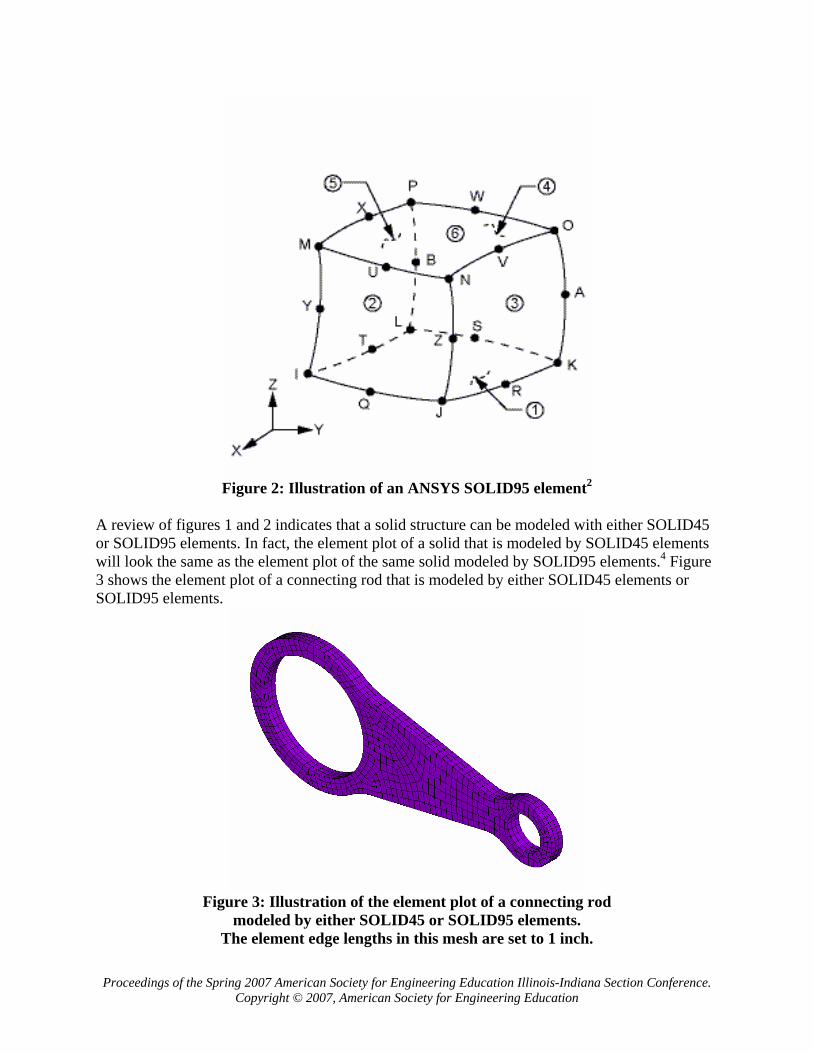
Figure 2: Illustration of an ANSYS SOLID95 element2

A review of figures 1 and 2 indicates that a solid structure can be modeled with either SOLID45 or SOLID95 elements. In fact, the element plot of a solid that is modeled by SOLID45 elements will look the same as the element plot of the same solid modeled by SOLID95 elements.4 Figure 3 shows the element plot of a connecting rod that is modeled by either SOLID45 elements or SOLID95 elements.

Figure 3: Illustration of the element plot of a connecting rod

modeled by either SOLID45 or SOLID95 elements. The element edge lengths in this mesh are set to 1 inch.


Every thing else being the same, a model made of SOLID45 elements takes less computer resources and runs faster than a model made of SOLID95 elements. However, SOLID45 elements are stiffer than SOLID95 elements in bending, and consequently, models made of SOLID45 elements are less accurate than models made of SOLID95 elements in areas where bending is present. Figure 4 shows the first scenario for the loading and support conditions for the finite element geometry and meshing shown in figure 3.

The left half of the connecting rod is modeled as fixed in all degrees of freedom.

A uniform pressure of 19000 PSI is applied to an area consisting of 40 degrees.

Figure 4: Illustration of the first loading and support conditions

scenario for the mesh of figure 3 Figure 5 is the stress contour for a finite element model using SOLID45 elements and meshed as shown in figure 3, and with support and loading conditions shown on figure 4.


Figure 5: Stress contour of models shown in figures 3 and 4

for a model made of SOLID45 elements. Figure 6 is the stress contour for a finite element model using SOLID95 elements and meshed as shown in figure 3, and with support and loading conditions shown on figure 4.

Figure 6: Stress contour of models shown in figures 3 and 4

for a model made of SOLID95 elements.


A review of figures 5 and 6 indicate a 5.75% difference in the maximum stress value for two models that are the same with the exception of the element type. ANSYS post processing has the capability of providing a plot indicating the structural element energy error for a given stress contour.3 Figure 7 is a plot of element energy error for the stress contour of figure 5 (SOLID45 elements), and figure 8 is a plot of element energy error for the stress contour of figure 6 (SOLID95) elements.

Figure 7: Energy error for stress contour of

figure 5 (SOLID45 elements)




A comparison of figures 7 and 8 indicate that for the model using SOLID95 elements, the estimated error is higher than the model using SOLID45 elements. This is an unexpected result, because it is generally agreed that SOLID95 is a more accurate element compared to SOLID45. However, in the case of loading of figure 4, the bending action is minimal because of the symmetry of loading and pressure. Figure 9 shows a support condition and a loading condition that produce a bending action for the geometry shown in figure 3.

The left half of the connecting rod is fixed for all degrees of freedom on the left of the model.

A uniform pressure of 12000 PSI is being applied over a 70 degree area as shown. This pressure combined with the supporting conditions creates a downward bending moment in the connecting rod.

Figure 9: Illustration of the second loading and support conditions

scenario for the mesh of figure 3 Figure 10 is the stress contour for the model of figure 9 where the solid is modeled using SOLID45 elements.


Figure 10: Stress contour for the model of figure 9

where SOLID45 elements were used

Figure 11 is the stress contour for the model of figure 9 where the solid is modeled using SOLID95 elements.

Figure 11: Stress contour for the model of figure 9

where SOLID95 elements were used


Figures 12 and 13 show the energy error levels for the stress contours of figures 10 and 11 respectively.






A review of figures 10 and 11 indicates a 6.94% difference in the maximum stress value for two models that are the same with the exception of the element type. A comparison of figures 12 and 13 indicate that for the loading condition of figure 9 the estimated error level for the stress contour produced by SOLID45 elements is higher than the stress contour produced by SOLID95 elements. There is a more severe bending action for the loading condition of figure 9 compared to the loading condition of figure 3. Consequently, the SOLID95 elements produced a more accurate finite element model for the loading condition of figure 9, since SOLID95 elements are more accurate than SOLID45 elements in bending. This result is the opposite of the results obtained for the loading condition of figure 3 where the estimated error levels for SOLID45 elements were lower than the SOLID95 elements. SOLID45 elements are more accurate than SOLID95 elements where the loading is axial or close to it. These comparisons illustrate the need for making the proper element selections for various loading conditions in order to obtain the most possible accurate results for a process that inherently is an approximate solution. The examples in this section demonstrate how the graphical representation of element energy error levels in ANSYS postprocessor can be an aid for optimizing the choice of elements used in a finite element model. Using ANSYS post processing error estimation capabilities for guidance in mesh density selection One of the issues in every finite element model is the appropriate choice of mesh density. If the mesh is not dense enough, the results of the finite element model will be inaccurate. On the other hand, if the mesh is unnecessarily too dense, it will lead to a waste of computer resources without any gain in the accuracy of the results. One of the techniques that can be used to estimate a suitable level for mesh density is the use of ANSYS post processor to graphically represent the element energy error levels.2 Figure 14 shows the same geometry meshed by SOLID45 elements using two different element edge lengths. The element edge length for the mesh on the left is 2.5 inches, and the element edge length for the mesh on the right is 1 inch.


Figure 14: Illustrations of the element plot of a connecting rod modeled by SOLID45 elements.

The element edge lengths on the left model is 2.5 inches. The element edge lengths on the right model is 1 inch.

The meshed models shown in figure 14 have been subjected to the support and loading conditions of figure 4 and the stresses were analyzed by the ANSYS finite element software. Figures 5 and 7 are the stress contour and the energy error contour for the right meshed model of figure 14 (element edge length of 1 inch). Figures 15 and 16 are the stress contour and the energy error contour for the left meshed model of figure 14 (element edge length of 2.5 inches).

Figure 15

Stress contour for the left meshed model of figure 14.


Figure 16

Energy error contour for the left meshed model of figure 14. A comparison of figures 5, 7, 15 and 16 indicate that the mesh sizes have significantly influenced the stress levels, and the energy error levels are higher when the element edge length has increased (when the mesh density has decreased). This indicates that the increase in element sizes (decrease in mesh density) has adversely affected the accuracy of the finite element model. While the examples demonstrated in this section are not conclusive, they demonstrate a possible technique where the graphical representation of element energy error levels feature of ANSYS postprocessor along with a comparison of stress contours (another graphics option in ANSYS) can provide some aid and guidance for optimizing the choice of element sizes in a finite element model. Graphical representation of normal vibration modes of a thin tube fixed at one end and rigid at the other end using PATRAN PATRAN is a graphics package that is capable of pre and post processing finite element models for a variety of finite element software packages. This example illustrates the use of PATRAN as a pre and post processor for NASTRAN finite element software.5

Figure 17 is a finite element model of a tube generated in PATRAN for a tube with a radius of 15 inches, a thickness of 0.125 inches and a length of 90 inches. The modulus of elasticity of the tube material is assumed to be 10E6 PSI, the Poisson’s ratio of the tube material is assumed to be 0.3, and the material density is assumed to be 0.101 pounds per cubic inch.


Figure 17: Finite element model of a tube fixed at one end and rigid at the free end

The normal free vibration modes of the tube shown in figure 17 are determined by using the NASTRAN finite element software. Table 1 is a summary of the frequencies for the first 10 modes of vibration for the tube obtained from the NASTRAN model.

Table 1 Natural frequencies for the 10 free vibration modes

of the tube of figure 17

Mode 1: 28 Hz Mode 2: 28 Hz Mode 3: 154 Hz Mode 4: 174 Hz Mode 5: 174 Hz Mode 6: 177 Hz Mode 7: 177 Hz Mode 8: 208 Hz Mode 9: 249 Hz Mode 10: 249 Hz

Figures 18 through 20 show the mode shapes for modes 1 through 3 defined in table 1. Figures 21 through 23 show the displacement contours for the first 3 mode shapes summarized in table 1. A review of figures 18 and 19 along with the information in table 1 show that modes 1 and 2 are basically the same modes. The NASTRAN finite element software is calculating them as two distinct modes because of geometric symmetry of the tube. Figures 21 and 22 confirm that modes 1 and 2 are the same modes. On the other hand figures 18 through 23 clearly demonstrate and confirm that the third calculated mode is different from modes 1 and 2.


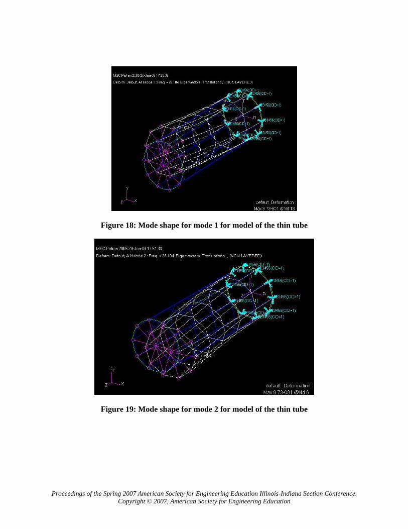
Figure 18: Mode shape for mode 1 for model of the thin tube




Figure 21: Displacement contour for mode 1 of the thin tube




The example in this section presents the use of PATRAN graphics package as a pre and post processor for NASTRAN finite element software. The example also illustrates how the PATRAN graphics package can enhance interpretation of the finite element results. Educational value of the techniques presented in this article The examples and techniques in this article demonstrate the use of graphical capabilities of ANSYS finite element software and PATRAN pre and post processor graphics software for


guiding and correcting finite element modeling efforts and for interpreting the results obtained through the use of the finite element modeling techniques. The techniques were demonstrated using relatively simple examples. In fact, an experienced engineer does not need to employ the demonstrated techniques to correctly model the structures shown in this article. However, the examples are useful for teaching the concept of using graphics to correctly use finite element software and to correctly interpret the results obtained through the use of finite element modeling. Once the techniques are mastered by the students, they can then be used in real life engineering scenarios where the use of the techniques are necessary for using finite element techniques correctly. The author is in the process of incorporating the techniques presented in this article in a graduate level distance learning finite element course that he teaches on a regular basis. Summary and Conclusion In this article two examples have been presented to demonstrate the use of ANSYS finite element software post processing graphics capabilities for developing better modeling practices and for interpreting the model results. Both of the ANSYS finite element models were static stress analysis models. The first ANSYS example demonstrated the use of graphical representation of element energy error level capabilities of ANSYS postprocessor as an aid for optimizing the choice of elements used in a finite element model. By using the demonstrated technique, the more accurate elements can be used where they are needed, and the less accurate elements can be used where such use provides the needed accuracy. The use of this approach will optimize the use of computer resources, since the more accurate elements also use more computer resources. The second ANSYS example demonstrated the use of ANSYS post processor graphical error estimating capabilities as an aid for choosing the optimal mesh size for a model. The use of such approach will also lead to a more optimal use of computer resources, since an excessively coarse mesh will lead to inaccurate finite element results, but an excessively fine mesh will waste computer resources without any meaningful gain in result accuracy. The article also presented an example on the use of PATRAN graphics package to develop a NASTRAN finite element model for vibration analysis, and then using the software for presenting and better interpreting the resulting free vibration modes. Bibliography 1. Section 4.45 of ANSYS Finite Element Software element reference manual. 2. Section 4.95 of ANSYS Finite Element Software element reference manual. 3. ANSYS Structural analysis guide section 2.3. 4. ANSYS Modeling and Meshing Guide. 5. MSC Software training course PAT301 notes.


Biography Dr. Hagigat is teaching undergraduate and graduate engineering technology courses at The University of Toledo. Dr. Hagigat has an extensive industrial background, and he is continuously emphasizing the practical applications of engineering topics covered in a typical engineering technology course.


Documents

USING FINITE ELEMENT SOFTWARE POST …ilin.asee.org/Conference2007program/Papers/Conference Papers... · This article presents examples of the use of ANSYS finite element software