Instrument Science Report ACS 2009-01

Updated CTE photometric correction for WFC and HRC

Marco Chiaberge, Pey Lian Lim, Vera Kozhurina-Platais, Marco Sirianni and Jennifer Mack

April 06, 2009

ABSTRACT

Observations for the ACS external CTE monitoring program were performed in Cycles 11 through 14 using both WFC and HRC. The aim of the program is to monitor the change in CTE in both cameras, and provide correction formulae for stellar photometry. Here we present the results of the data analysis, and we provide correction formulae for photometry on drizzled images for both HRC and WFC. The correction formulae we present here are significantly more accurate than those previously published, both because of the larger amount of data available and because of a more advanced analysis strategy. Observers are encouraged to use the new formulae to correct photometry, especially in presence of faint stars on a low sky background.

IntroductionOne of the effects of radiation damage on CCD in space is a decrease in the Charge Transfer Efficiency (CTE). This is explained in terms of an increase of charge traps in the CCD due to proton irradiation in the space environment. CTE is defined as (1-CTI), where CTI = ∆Q/Q is the fractional charge lost during each single transfer (Charge Transfer Inefficiency).

Since 2003, specific calibration programs aimed at characterizing the effects of the CTE on stellar photometry were performed (Riess, ISR ACS 2003-009). First characterizations of the effects of a decreasing CTE for WFC were made by Riess & Mack (IRS ACS 2004-006). Meanwhile, results from the internal CTE calibration programs showed that CTE appears to decline linearly with time, and that CTE losses are stronger for lower signal levels (Mutchler & Sirianni ISR 2005-03). However, in order to derive an accurate correction

1Operated by the Association of Universities for Research in Astronomy, Inc., for the National Aeronautics and Space Administration

formula for photometry, a number of observations at different epochs and for different levels of sky background and stellar fluxes have to be accumulated. In this ISR, we show the results of the observations taken through March 2006, which, coupled with a different approach in the data analysis, allowed us to significantly improve the CTE photometric correction formulae for both WFC and HRC.

ObservationsThe observations were taken as part of calibration programs CAL/ACS 9648, 10043, 10368 (PI: A. Riess), 10730 (PI: M. Chiaberge). A detailed description of the observational strategy can be found in Riess (ISR ACS 2003-009). The target of the observing program is a field ~6’ West off the core of the globular cluster 47 Tucanae for WFC and a different field, located about ~5’ NW off the cluster’s core, for HRC. We image the field with WFC at the initial position, and then we utilize 2 large slews (102”), i.e. half the size of the WFC. The slews are performed both in the X and in the Y directions in the detector framework, to vary the number of transfers for each star in the field, and check serial and parallel CTE, respectively. For reference, in Fig. 1 we reprint a figure from Riess (ISR ACS 2003-009) which illustrates the observing strategy. For example, a star located at Y=100 in the FLT file framework when observed with WFC2 (image at position “0,0”), will also fall at Y=100 when observed on WFC1 after the slew is performed (image position “0,1”). However, the star undergoes Y-transfersWFC2=100 and Y-transfers WFC1=2048-100 when it is read out from WFC2 and WFC1, respectively. Such a pair of images is used to check parallel CTE, by comparing the measured magnitudes of stars in the two images. For serial CTE, the shift is performed in the X direction, and the images “0,0” and “1,0” are used. For the HRC, the number of transfers for each star is varied simply using different amplifiers for readout (A and C to check parallel CTE, C and D for serial).

Images are taken with 3 different filters (F502N, F606W and F775W) and different exposure times, in order to sample different background levels. Short and long exposures are taken: 30s and 400s for all filters and WFC; 30s and 360s are used for F606W and F775W on the HRC, while for F502N only a long (360s) exposure is performed.

2

Figure 1: The location of the 4 WFC amplifiers and the readout direction are reported in the left panel of the figure. In the right panel, we show a schematic of the 2 dither positions used to check parallel CTE (repreinted from Riess ISR ACS 2003-009).

The data are single images, and neither CR-SPLIT nor dithering were performed. As a result of that, the images are strongly contaminated by cosmic rays and hot pixels (as well as saturated pixels because of the presence of bright stars in the field), which limit the number of stars for which a reliable comparison between the measured flux in the different images can be performed. In Fig 2 we show a section of ~30”x30” in the WFC field (F606W, exp time = 300s) as an example.

In the following we outline our analysis procedure for both HRC and WFC, we present results for single epochs and we derive improved time dependent formulae to correct aperture photometry for point sources.

3

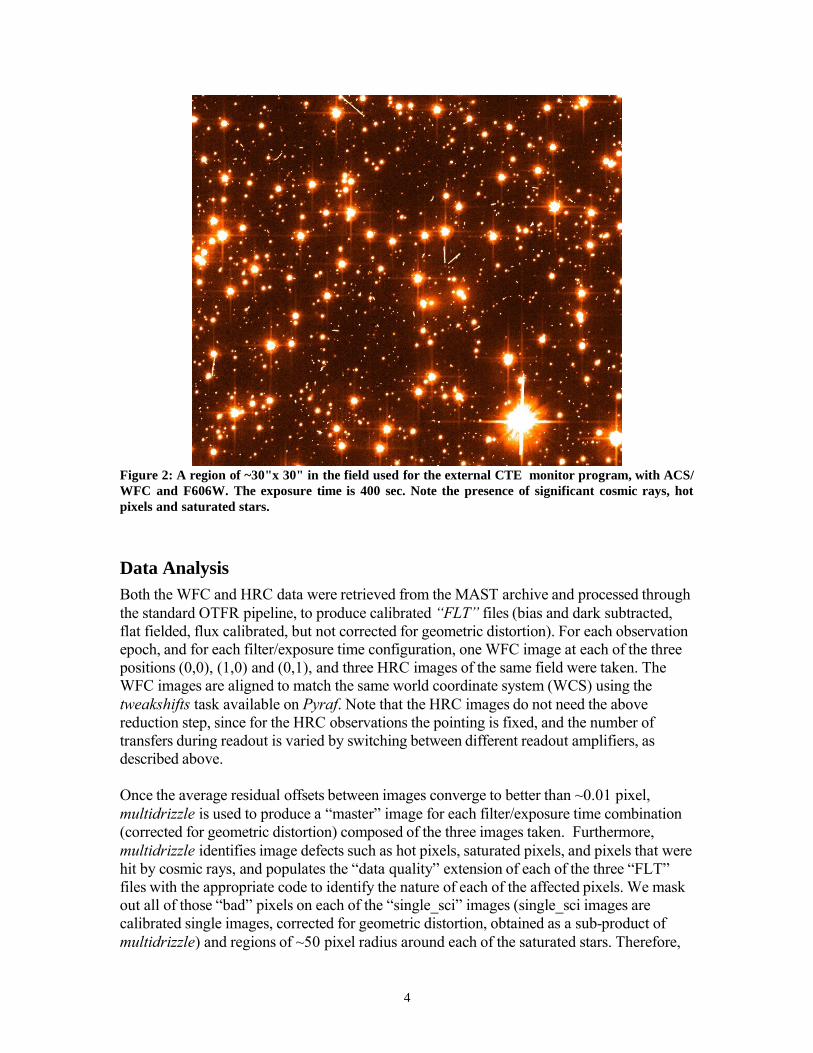
Figure 2: A region of ~30"x 30" in the field used for the external CTE monitor program, with ACS/WFC and F606W. The exposure time is 400 sec. Note the presence of significant cosmic rays, hot pixels and saturated stars.

Data Analysis Both the WFC and HRC data were retrieved from the MAST archive and processed through the standard OTFR pipeline, to produce calibrated “FLT” files (bias and dark subtracted, flat fielded, flux calibrated, but not corrected for geometric distortion). For each observation epoch, and for each filter/exposure time configuration, one WFC image at each of the three positions (0,0), (1,0) and (0,1), and three HRC images of the same field were taken. The WFC images are aligned to match the same world coordinate system (WCS) using the tweakshifts task available on Pyraf. Note that the HRC images do not need the above reduction step, since for the HRC observations the pointing is fixed, and the number of transfers during readout is varied by switching between different readout amplifiers, as described above.

Once the average residual offsets between images converge to better than ~0.01 pixel, multidrizzle is used to produce a “master” image for each filter/exposure time combination (corrected for geometric distortion) composed of the three images taken. Furthermore, multidrizzle identifies image defects such as hot pixels, saturated pixels, and pixels that were hit by cosmic rays, and populates the “data quality” extension of each of the three “FLT” files with the appropriate code to identify the nature of each of the affected pixels. We mask out all of those “bad” pixels on each of the “single_sci” images (single_sci images are calibrated single images, corrected for geometric distortion, obtained as a sub-product of multidrizzle) and regions of ~50 pixel radius around each of the saturated stars. Therefore,

4

stars affected by artifacts of any kind are effectively rejected and photometry is performed on “clean” stars only.

We perform aperture photometry on a star list obtained by running the task daofind in the IRAF package daophot on the “master” image. Stars from the complete list are then re-centered on each of the single_sci images, and photometry is performed using the task phot, after rejection of all stars that are contaminated by cosmic rays and/or hot pixels. The photometry aperture radius is set to 3 pixels for both HRC and WFC. This ensures that reliable aperture photometry can be performed on both faint and bright stars. Furthermore, the number of rejected stars would significantly increase for larger aperture, because a higher number of pixels flagged as “bad” would be included in the aperture. A low number of stars would hamper the accurate measurement of the CTE effect with the aim of deriving a correction formula. The background is measured locally, in an annulus of inner radius r=13 pixels and d=3 pixels wide for WFC, while r=15 and d=4 for the HRC.

In the following, we focus mainly on parallel CTE (i.e. CTE in the y-direction). However, we checked that for both WFC and HRC, the CTE effect in the x-direction (serial CTE) is negligible in our data, as of March 2006 (see below).

For each epoch, filter and exposure time combination, stellar fluxes measured in each “pair” of images are grouped in bins of magnitude. Usually, 6 and 4 bins are obtained for WFC and HRC, respectively. Bright stars in the field used for the observations increase the background level over large regions across the images. Since the CTE depends strongly on the background level, we restrict the analysis to stars in a narrow range of background levels. For a few configurations, we have enough stars in the field to allow more than one bin of sky levels. For each bin of flux level and sky background, the magnitude difference between stars as measured in each pair of images (positions “0,0” and “0,1”) ∆mag = m0 – m1 is plotted against the number of Y-transfers each star undergoes during read out. More precisely, Y-transfers ≡ ∆Y-transfers = Y-transfers0 -Y-transfers1, i.e. the difference between the number of transfers in the two images, is used. A linear fit to the data is performed, and outliers are rejected using iterative sigma-clipping. After four iterations, the value of ∆mag2000 i.e. the value of ∆mag for 2000 pixel transfers (1000 transfers for the HRC) is derived from the slope of the linear regression. In the following, we show results for WFC and HRC from single epoch observations, and we discuss the method to derive time-dependent correction formulae.

5

Results for WFC

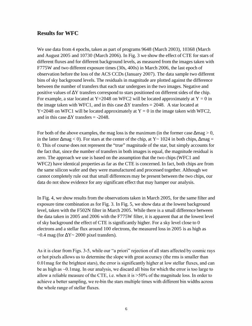
We use data from 4 epochs, taken as part of programs 9648 (March 2003), 10368 (March and August 2005 and 10730 (March 2006). In Fig. 3 we show the effect of CTE for stars of different fluxes and for different background levels, as measured from the images taken with F775W and two different exposure times (30s, 400s) in March 2006, the last epoch of observation before the loss of the ACS CCDs (January 2007). The data sample two different bins of sky background levels. The residuals in magnitude are plotted against the difference between the number of transfers that each star undergoes in the two images. Negative and positive values of ∆Y transfers correspond to stars positioned on different sides of the chip. For example, a star located at Y=2048 on WFC2 will be located approximately at Y = 0 in the image taken with WFC1, and in this case ∆Y transfers = 2048. A star located at Y=2048 on WFC1 will be located approximately at Y = 0 in the image taken with WFC2, and in this case ∆Y transfers = -2048.

For both of the above examples, the mag loss is the maximum (in the former case ∆mag > 0, in the latter ∆mag < 0). For stars at the center of the chip, at Y~ 1024 in both chips, ∆mag = 0. This of course does not represent the “true” magnitude of the star, but simply accounts for the fact that, since the number of transfers in both images is equal, the magnitude residual is zero. The approach we use is based on the assumption that the two chips (WFC1 and WFC2) have identical properties as far as the CTE is concerned. In fact, both chips are from the same silicon wafer and they were manufactured and processed together. Although we cannot completely rule out that small differences may be present between the two chips, our data do not show evidence for any significant effect that may hamper our analysis.

In Fig. 4, we show results from the observations taken in March 2005, for the same filter and exposure time combination as for Fig. 3. In Fig. 5, we show data at the lowest background level, taken with the F502N filter in March 2005. While there is a small difference between the data taken in 2005 and 2006 with the F775W filter, it is apparent that at the lowest level of sky background the effect of CTE is significantly higher. For a sky level close to 0 electrons and a stellar flux around 100 electrons, the measured loss in 2005 is as high as ~0.4 mag (for ∆Y~ 2000 pixel transfers).

As it is clear from Figs. 3-5, while our “a priori” rejection of all stars affected by cosmic rays or hot pixels allows us to determine the slope with great accuracy (the rms is smaller than 0.01mag for the brightest stars), the error is significantly higher at low stellar fluxes, and can be as high as ~0.1mag. In our analysis, we discard all bins for which the error is too large to allow a reliable measure of the CTE, i.e. when it is >50% of the magnitude loss. In order to achieve a better sampling, we re-bin the stars multiple times with different bin widths across the whole range of stellar fluxes.

6

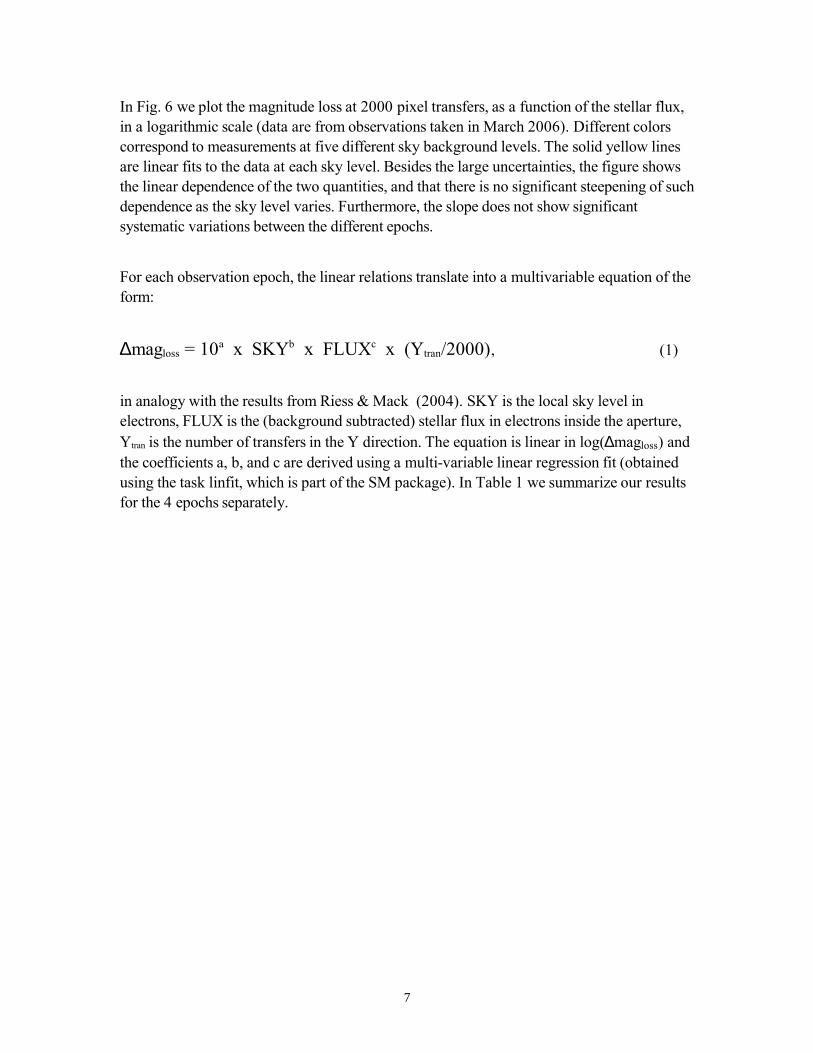
In Fig. 6 we plot the magnitude loss at 2000 pixel transfers, as a function of the stellar flux, in a logarithmic scale (data are from observations taken in March 2006). Different colors correspond to measurements at five different sky background levels. The solid yellow lines are linear fits to the data at each sky level. Besides the large uncertainties, the figure shows the linear dependence of the two quantities, and that there is no significant steepening of such dependence as the sky level varies. Furthermore, the slope does not show significant systematic variations between the different epochs.

For each observation epoch, the linear relations translate into a multivariable equation of the form:

∆magloss = 10a x SKYb x FLUXc x (Ytran/2000), (1)

in analogy with the results from Riess & Mack (2004). SKY is the local sky level in electrons, FLUX is the (background subtracted) stellar flux in electrons inside the aperture, Ytran is the number of transfers in the Y direction. The equation is linear in log(∆magloss) and the coefficients a, b, and c are derived using a multi-variable linear regression fit (obtained using the task linfit, which is part of the SM package). In Table 1 we summarize our results for the 4 epochs separately.

7

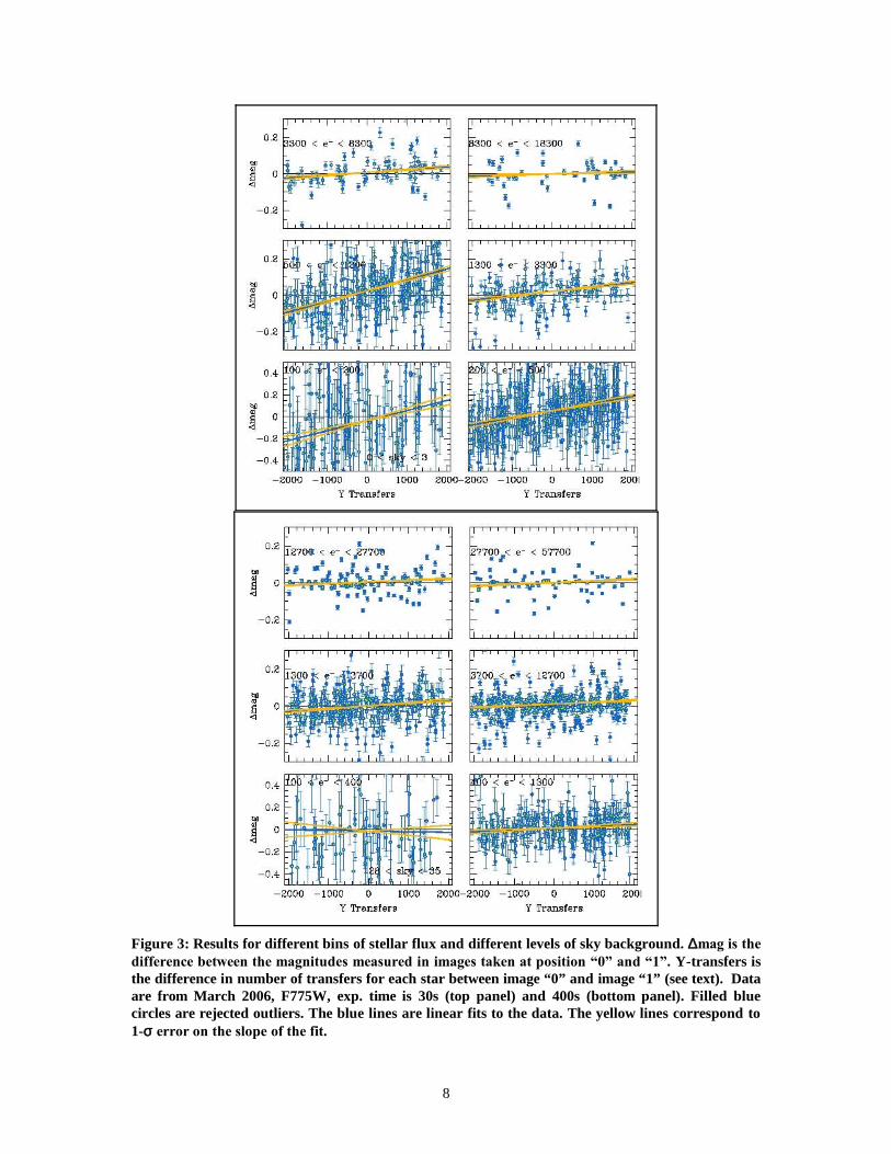
Figure 3: Results for different bins of stellar flux and different levels of sky background. ∆mag is the difference between the magnitudes measured in images taken at position “0” and “1”. Y-transfers is the difference in number of transfers for each star between image “0” and image “1” (see text). Data are from March 2006, F775W, exp. time is 30s (top panel) and 400s (bottom panel). Filled blue circles are rejected outliers. The blue lines are linear fits to the data. The yellow lines correspond to 1-σ error on the slope of the fit.

8

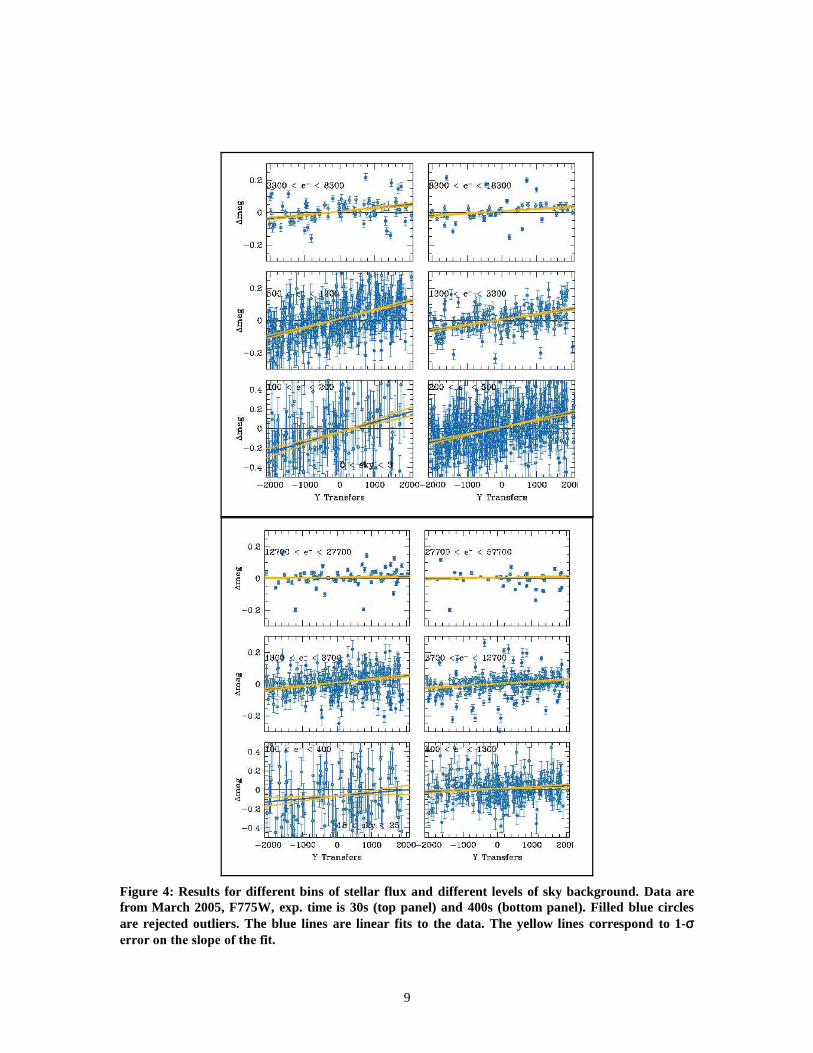
Figure 4: Results for different bins of stellar flux and different levels of sky background. Data are from March 2005, F775W, exp. time is 30s (top panel) and 400s (bottom panel). Filled blue circles are rejected outliers. The blue lines are linear fits to the data. The yellow lines correspond to 1-σ error on the slope of the fit.

9

Figure 5: Results for different bins of stellar flux and the lowest sky background levels. Data were taken with the F502N filter, 30s (top) and 400s (bottom) exposure time in March 2005. Filled blue circles are rejected outliers. The blue lines are linear fits to the data. The yellow lines correspond to 1-σ error on the slope of the fit.

10

Figure 6: Log of the magnitude loss at 2000 transfers vs. log of stellar flux (in electrons). Dots of different colors correspond to bins of different sky levels. Blue corresponds to a sky level < 1 e-, light red is for 1 < e- < 3, black is for 3 < e- < 10, yellow is for 10 < e- < 35 while red corresponds to sky ~ 45 e-. The solid lines are linear fits to the data for each sky level, which is identified by the line color. The error bars on the Flux axis correspond to the width of each flux bin. Data are from the observations taken in March 2006.

Table 1: Coefficients for WFC at each observation epoch

Mar 2003 Mar 2005 Aug 2005 Mar 2006a -0.12 ± 0.20 0.34 ± 0.06 0.38 ± 0.09 0.43 ± 0.11b -0.36 ± 0.14 -0.22 ± 0.02 -0.26 ± 0.02 -0.26 ± 0.03c -0.44 ± 0.05 -0.44 ± 0.02 -0.47 ± 0.05 -0.47 ± 0.03

11

Time dependent formula for WFC

We assume that ∆magloss = 0 for all star fluxes, sky levels and number of transfers at the time of launch (MJD=52333), in analogy with Riess & Mack (2004). Although this is not formally correct, since it implies that CTE = 1 at that time, it is still a reasonable assumption (see e.g. Golimowski et al 2000, Mutchler & Sirianni 2005 for pre-launch tests results and results based on in-flight internal CTE tests). We also assume a linear dependence of the CTE degradation with time, based both on previous experience with WFPC2 and STIS and on the results of internal tests (Mutchler & Sirianni 2005). These assumptions allow us to derive a time dependent formula of the form

∆magloss = 10γ x SKYb x FLUXc x (Ytran/2000) x (MJD-52333)/365, (2)

again in analogy with Riess & Mack (2004).

The “γ”coefficient is the equivalent of the “a” coefficient in (1), but it is free of any dependence on time. The value of the “γ”coefficient is derived for each epoch. Then the values at each epoch for the three coefficients γ, b and c are averaged using a weighted mean formula. The errors on the weighted mean values are estimated with the weighted variance. In Table 2 we report the final values of the coefficients, and their estimated error.

The magnitude losses we measured, which are accounted for by our newly derived photometric correction formula (2), are on average a factor of ~2 higher than those predicted with the formula of Riess & Mack (2004). However, because of the large uncertainty of that formula, which was based on a limited number of images and observing epochs, the results of both formulae agree in most cases (within 1σ). Our new results are significantly more accurate because of both the larger amount of data and because of the more advanced data analysis strategy. The typical rms error on the magnitude losses obtained with the new correction formula we derived is about a factor of 2 smaller than the Riess & Mack (2004) formula, depending on the values of the stellar flux and the sky background level.

Table 2: Weighted mean value of the coefficients in the CTE correction formula for WFC and aperture photometry (aperture radius r= 3 pix) of stars in “drizzled” images.

Weighted Mean

σ

γ -0.15 0.04

B -0.25 0.01

C -0.44 0.02

12

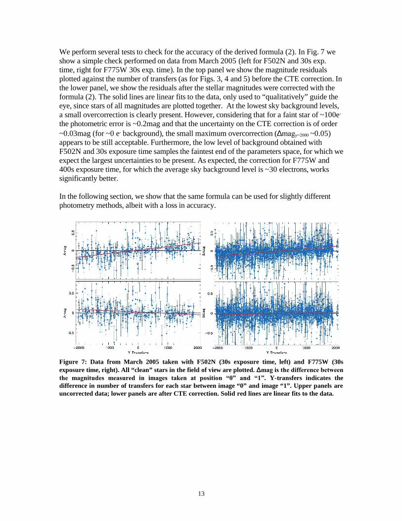
We perform several tests to check for the accuracy of the derived formula (2). In Fig. 7 we show a simple check performed on data from March 2005 (left for F502N and 30s exp. time, right for F775W 30s exp. time). In the top panel we show the magnitude residuals plotted against the number of transfers (as for Figs. 3, 4 and 5) before the CTE correction. In the lower panel, we show the residuals after the stellar magnitudes were corrected with the formula (2). The solid lines are linear fits to the data, only used to “qualitatively” guide the eye, since stars of all magnitudes are plotted together. At the lowest sky background levels, a small overcorrection is clearly present. However, considering that for a faint star of ~100e-

the photometric error is ~0.2mag and that the uncertainty on the CTE correction is of order ~0.03mag (for ~0 e- background), the small maximum overcorrection (∆magy=2000 ~0.05) appears to be still acceptable. Furthermore, the low level of background obtained with F502N and 30s exposure time samples the faintest end of the parameters space, for which we expect the largest uncertainties to be present. As expected, the correction for F775W and 400s exposure time, for which the average sky background level is ~30 electrons, works significantly better.

In the following section, we show that the same formula can be used for slightly different photometry methods, albeit with a loss in accuracy.

Figure 7: Data from March 2005 taken with F502N (30s exposure time, left) and F775W (30s exposure time, right). All “clean” stars in the field of view are plotted. ∆mag is the difference between the magnitudes measured in images taken at position “0” and “1”. Y-transfers indicates the difference in number of transfers for each star between image “0” and image “1”. Upper panels are uncorrected data; lower panels are after CTE correction. Solid red lines are linear fits to the data.

13

CTE correction formula for different photometric methods

The photometric correction formula has been derived using aperture photometry on drizzled files, and the aperture radius has been set to r = 3pix for the reasons explained above. However, we checked whether the same formula can be used to correct stellar photometry derived using different methods, i.e. 1) aperture photometry with different aperture radii, 2) aperture photometry on flat-fielded (“FLT”) files and 3) psf fitting using the ePSF code (Anderson 2006). In the following we describe the results of various tests we performed.

Aperture photometry

We performed tests using aperture radii of 1.5 and 5 pixels and then correcting the photometry utilizing the formula we derived for r = 3 pixels. We show the results in Figs. 8 and 9. In Fig 8, we show data taken with F775W in March 2005. Photometry is performed with r = 1.5 pixels. The median background level is about 2 e-. Therefore, for each bin of stellar flux, the CTE is close to its lowest level (i.e. the magnitude loss is large). We applied the photometric correction formula regardless of the different aperture radius. The comparison between the data for different bins of stellar flux before and after correction is shown in Fig. 8 (left and right panels, respectively). Some undercorrection is seen for some of the bins. The maximum undercorrection (residual ∆magy=2000 = 0.04) occurs for the bin for which the stellar flux is the lowest (between 50 e- and 100 e-). However, note that the rms error on the linear fit in that case is σ = 0.03 and the photometric error for stars of such a low flux is significantly larger than the residual ∆mag. We also found similar results for different levels of sky background. Thus we conclude that the photometric correction formula can be used for aperture photometry with r = 1.5 pixels, in case the users prefer a smaller aperture to the “standard” r = 3 pixels.

A similar result holds for r = 5 pixel aperture. In case the user prefers a larger aperture radius (which is however not recommended, especially in case of faint stars), the correction formula can still be used. In this case it’s hard to break down stars into different bins of flux, because the total number of stars not affected by cosmic rays or hot pixels is low. However, Fig. 9 shows that considering all available stars in the field of view the correction works quite well, leading to a cumulative ∆magy=2000 ~ 0.0 mag after correction, for the particular case shown. Similar results are obtained for the other filter/exposure time combinations.

14

Figure 8: Aperture photometry with aperture radius r = 1.5 pixels. Data are from March 2005, F775W, 30s exposure time. Uncorrected photometry is shown in the top panel, while in the bottom panel we show the same data after CTE correction (see caption of Fig 3 and text for more details). The red lines are linear fits to the data, yellow lines. The yellow lines in the top panel correspond to 1-σ error on the slope of the fit.

15

Figure 9: Aperture photometry with aperture radius r = 5 pixels. Data are from March 2005 epoch, F775W, 30s exposure time. Uncorrected photometry is shown in the top panel, while in the lower panel we show the same data after CTE correction. All available stars in the field of view are plotted. The red solid lines are linear fits to the data. The residual ∆magy=2000 after correction is compatible with 0.0mag.

Aperture photometry and PSF fitting on FLT files

We used images taken as part of the CTE calibration programs to obtain “effective PSF” (ePSF) fitting photometry and aperture photometry from flat-fielded “FLT” images with the img2xym_WFC.09x10 FORTRAN code (Anderson & King 2006). The same code was successfully used to derive the differential correction of CTE-induced photometric loss and centroid shift, by comparison of long and short exposures from a specific dataset (Kozhurina-Platais et al. ISR 2007-04). The code returns a list of (X,Y) positions and fluxes for stars in the images. The measured star positions were corrected for geometric distortion applying the ACS/WFC distortion model of Anderson & King (2006). Subsequently, X,Y coordinates of stars from one pointing (0,0) were matched with the positions from pointing (0,1), using the general 6 parameter linear transformation and utilizing a least-square minimization, iteratively rejecting CR, hot pixels and outliers. The rejection method here assumes that cosmic ray hits and hot pixels affect the position of stars. Therefore, stars whose positions do not match to better than ~0.1 pixels are rejected.

We used the img2xym_WFC.09x10 code to perform both ePSF fitting photometry and aperture photometry with aperture radius of r=3 pixels, measuring the sky in an annulus between r=10 and 15 pixels. In Fig. 10 we show the magnitude residuals ∆m between short (30s) and long (400s) exposures, as measured with ePSF fitting using aperture photometry (bottom) and PSF fitting (top). The residuals are plotted against the Y coordinate of the stars

16

in the FLT framework. Note that this is different from the previous figures: in this case the amplifiers are located at Y=0 and Y=4096, therefore we expect ∆mag=0 for Y=0 and Y=4096, and the maximum value of ∆mag is expected at the center of the plot, for Y~2048. Data are from the images taken with the F606W filter in March 2006. In the left panels, we show the data before CTE correction and in the right panels after CTE correction. Qualitatively, there is a clear improvement after applying the photometric correction in both cases. The correction gives slightly better results for aperture photometry, as one may expect, but appears to work well for PSF fitting too. We also considered bins of stellar flux and we did not find any particular regime for which the correction works worse than for others.

Figure 10: Magnitude residuals between short (30s) and long (400s) exposures (∆m), as measured with the img2xym_WFC.09x10 code, plotted vs the Y coordinate in the framework of the FLT files. The data are from March 2006 and were taken using the F606W filter. In the bottom panels photometry is performed using aperture photometry, while in top panels photometry is performed with ePSF fitting. The left panels correspond to no CTE correction, while the right panels show the residuals after CTE correction using the formula presented in this ISR. The red line represents ∆m=0.

We also checked for magnitude residuals between stars measured with ePSF fitting in the two WFC chips, using the half-size field-of-view slews to vary the number of transfers in the Y direction, as for the “standard” aperture photometry procedure described in the previous sections. The results are shown in Fig 11 where we plot the magnitude residuals against the Y coordinate of the star in the WFC2 chip. These plots are similar to the ones in e.g. Fig. 9, since the expectation is to observe maximum (either positive or negative) ∆mag at the edges of each plot (i.e for Y=2049 and Y=4096 in Fig .11). For stars located at the center of each chip (corresponding to Y=3072 in Fig. 11) we expect ∆mag=0. In the example shown here (see right panel), a small (~0.05mag) overcorrection for stars that undergo ~2000 pixel transfers is apparent. Note that, in this particular case, the overcorrection is approximately

17

the same as the error resulting from not correcting the photometry, but in the opposite direction.

Based on the checks we performed, we point out that the correction formula (2) can be used to correct photometry obtained with methods other than aperture photometry on drizzled files, albeit with a lower level of accuracy. Not surprisingly, the most accurate results are obtained when aperture photometry is performed. However, a detailed comparison between the results obtained using different photometry methods is beyond the scope of this paper.

Figure 11: Residuals between star magnitudes ∆m measured with ePSF fitting in the two WFC chips, using the half-field-of-view slews to vary the number of transfers along the Y direction. Y coordinates refer to coordinates in the framework of the flt files. The Y coordinate of the star in the WFC2 chip is plotted. Data taken with the F775W and 30s exposure time are used. In the left panel we show the residuals before CTE correction, in the right panel after CTE correction. The red line is a linear fit to the data.

Results for the HRCIn order to derive a correction formula for the HRC we used an approach similar to that used for the WFC. However, as explained above, for the HRC we vary the number of transfers each star undergoes by using different readout amplifiers for each image (amplifiers A and C are used to check for parallel CTE), while the pointing is fixed. We use data from 4 epochs, August 2004, March and August 2005, and March 2006, from programs 10043, 10368 and 10730, respectively. The low number of stars in the observed field makes the measurement of CTE more difficult. Therefore, we discarded data from epochs previous to 2005, in order to deal with datasets in which the effect of CTE degradation is maximized. Aperture photometry on the drizzled files is performed as for the WFC, using an aperture radius of 3 pixels.

In Fig. 12 we show results from March 2006 observations (program 10730). The observations were taken with the F502N and F775W filters (300s and 30s exposure time, respectively) which result in a low sky background level. “∆Y-transfers” indicates the difference in number of transfers for each star between images read out with two different amplifiers. ∆mag is the difference between the magnitudes measured in the two images. The

18

blue dotted line is the linear fits to the data; the blue solid line is the same as the dotted line, but shifted so that ∆mag = 0 at ∆Y Transfers = 0, for the sake of clarity. The yellow lines correspond to 1-σ error on the slope of the fit. We also plot as black solid lines the prediction obtained using the previously published CTE correction formula in the ACS Handbook, and the 1-σ error on the slope, for comparison. The previously published formula was based on one observation epoch only, thus its large uncertainty is not surprising. In Fig. 13, we show data from the same epoch (March 2006) but for a higher bin of sky background, since the images were obtained using the F606W and F775W filters and 300s exposure times.

In order to measure the CTE effect on stellar photometry for the HRC we use the same method as for the WFC, i.e. we perform aperture photometry on drizzled images, setting the aperture radius to r=3 pixels and measuring the background locally, in an annulus of inner radius r=15 pixels and thickness d=4 pixels. For each epoch we measure the CTE loss for 1000 pixel transfers, for different bins of stellar flux and sky background. Then we perform a multivariable regression analysis to derive the coefficients of the formula that is assumed to be of the form of equation (1), modified to account for the smaller detector size (eq. 3). We derive the parameters for the correction formula at each observational epoch, which are reported in Table 3.

∆magloss = 10a x SKYb x FLUXc x (Ytran/1000) (3)

19

Figure 12: Results from March 2006 observing epoch. The data are from observations with the F775W filter and 30s exposure time (left) and F502N and 300s exp. time (right). ∆mag is the difference between the magnitudes measured in images taken at position “0” and “1”. ∆Y-transfers is the difference in number of transfers for each star between images read out with two different amplifiers (A and C). In each box, the blue dotted line is the linear fit to the data; the blue solid line is the same as the dotted line, but shifted so that ∆mag=0 at ∆Y Transfers = 0. The yellow lines correspond to 1-σ error on the slope. The black solid lines are the predictions obtained using the previously published CTE correction formula in the ACS Handbook and their 1-σ error. Blue dots represent rejected outliers.

20

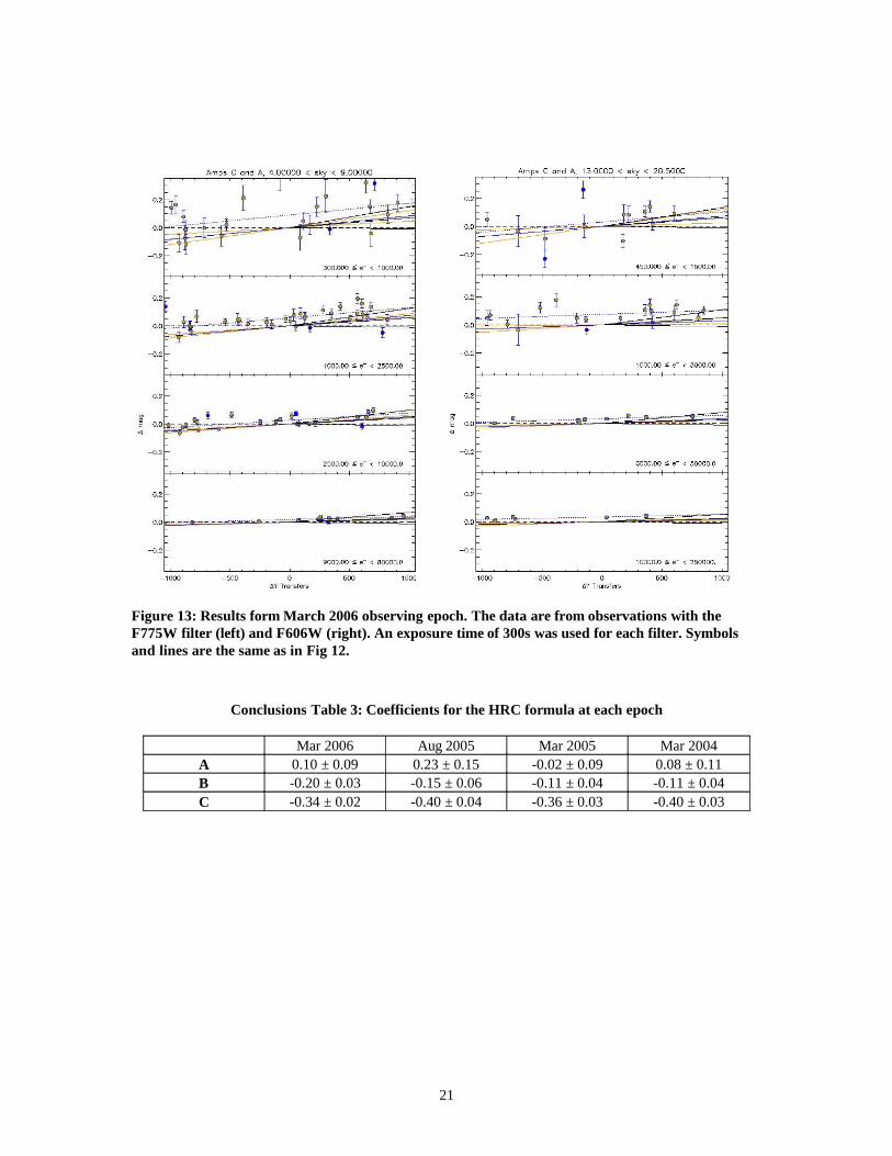
Figure 13: Results form March 2006 observing epoch. The data are from observations with the F775W filter (left) and F606W (right). An exposure time of 300s was used for each filter. Symbols and lines are the same as in Fig 12.

Conclusions Table 3: Coefficients for the HRC formula at each epoch

Mar 2006 Aug 2005 Mar 2005 Mar 2004A 0.10 ± 0.09 0.23 ± 0.15 -0.02 ± 0.09 0.08 ± 0.11B -0.20 ± 0.03 -0.15 ± 0.06 -0.11 ± 0.04 -0.11 ± 0.04C -0.34 ± 0.02 -0.40 ± 0.04 -0.36 ± 0.03 -0.40 ± 0.03

21

Under the same assumption as for the WFC (i.e. CTE = 1 at the time of launch), we derive the following time-dependent correction formula, in analogy with Riess & Mack (2004):

∆magloss = 10γ x SKYb x FLUXc x (Ytran/1000) x (MJD-52333)/365. (4)

The values of the coefficients are reported in Table 4.

Table 4: Weighted mean value of the coefficients in the CTE correction formula for the HRC and aperture photometry (aperture radius r= 3 pix) of stars in “drizzled” images.

Weighted Mean

σ

γ -0.44 0.05

B -0.15 0.02

C -0.36 0.01

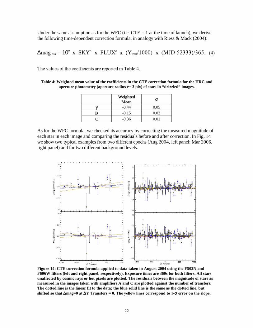
As for the WFC formula, we checked its accuracy by correcting the measured magnitude of each star in each image and comparing the residuals before and after correction. In Fig. 14 we show two typical examples from two different epochs (Aug 2004, left panel; Mar 2006, right panel) and for two different background levels.

Figure 14: CTE correction formula applied to data taken in August 2004 using the F502N and F606W filters (left and right panel, respectively). Exposure times are 360s for both filters. All stars unaffected by cosmic rays or hot pixels are plotted. The residuals between the magnitude of stars as measured in the images taken with amplifiers A and C are plotted against the number of transfers. The dotted line is the linear fit to the data; the blue solid line is the same as the dotted line, but shifted so that ∆mag=0 at ∆Y Transfers = 0. The yellow lines correspond to 1-σ error on the slope.

22

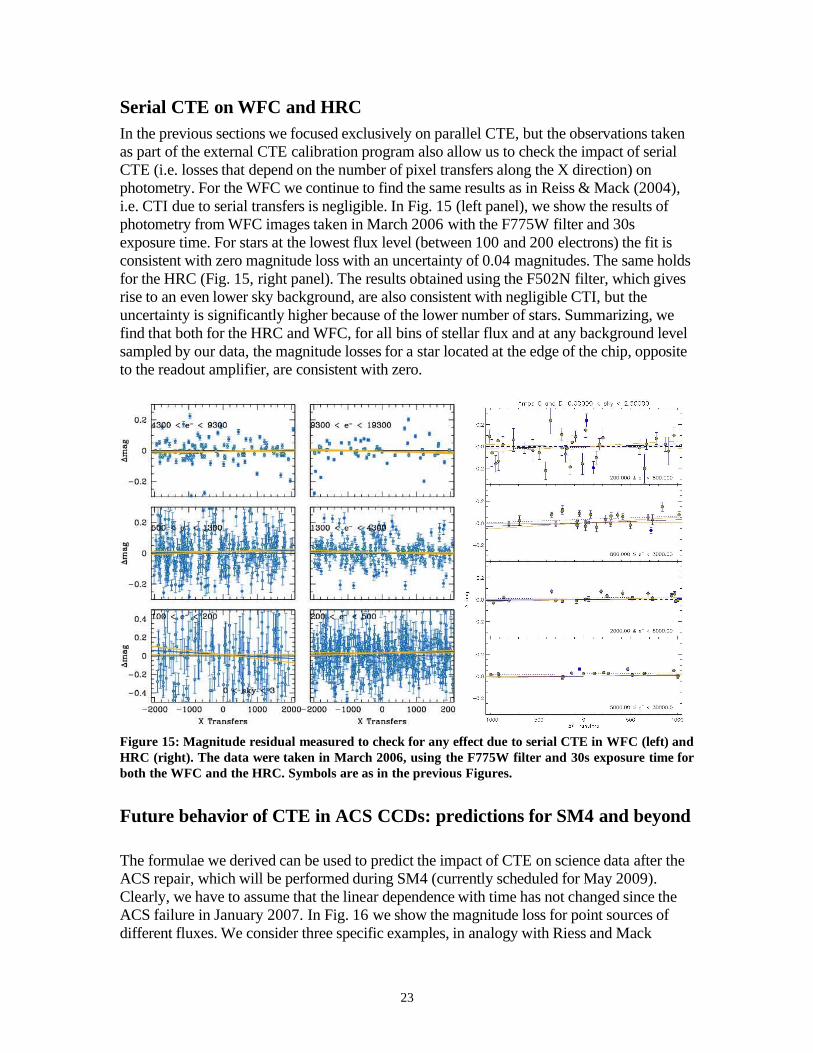
Serial CTE on WFC and HRCIn the previous sections we focused exclusively on parallel CTE, but the observations taken as part of the external CTE calibration program also allow us to check the impact of serial CTE (i.e. losses that depend on the number of pixel transfers along the X direction) on photometry. For the WFC we continue to find the same results as in Reiss & Mack (2004), i.e. CTI due to serial transfers is negligible. In Fig. 15 (left panel), we show the results of photometry from WFC images taken in March 2006 with the F775W filter and 30s exposure time. For stars at the lowest flux level (between 100 and 200 electrons) the fit is consistent with zero magnitude loss with an uncertainty of 0.04 magnitudes. The same holds for the HRC (Fig. 15, right panel). The results obtained using the F502N filter, which gives rise to an even lower sky background, are also consistent with negligible CTI, but the uncertainty is significantly higher because of the lower number of stars. Summarizing, we find that both for the HRC and WFC, for all bins of stellar flux and at any background level sampled by our data, the magnitude losses for a star located at the edge of the chip, opposite to the readout amplifier, are consistent with zero.

Figure 15: Magnitude residual measured to check for any effect due to serial CTE in WFC (left) and HRC (right). The data were taken in March 2006, using the F775W filter and 30s exposure time for both the WFC and the HRC. Symbols are as in the previous Figures.

Future behavior of CTE in ACS CCDs: predictions for SM4 and beyond

The formulae we derived can be used to predict the impact of CTE on science data after the ACS repair, which will be performed during SM4 (currently scheduled for May 2009). Clearly, we have to assume that the linear dependence with time has not changed since the ACS failure in January 2007. In Fig. 16 we show the magnitude loss for point sources of different fluxes. We consider three specific examples, in analogy with Riess and Mack

23

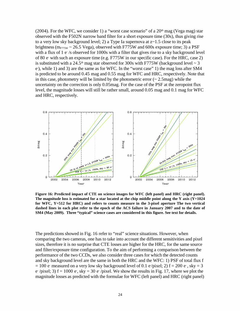
(2004). For the WFC, we consider 1) a “worst case scenario” of a 20th mag (Vega mag) star observed with the F502N narrow band filter for a short exposure time (30s), thus giving rise to a very low sky background level; 2) a Type Ia supernova at z~1.5 close to its peak brightness (mF775W ~ 26.5 Vega), observed with F775W and 600s exposure time; 3) a PSF with a flux of 1 e- /s observed for 1000s with a filter that gives rise to a sky background level of 80 e- with such an exposure time (e.g. F775W in our specific case). For the HRC, case 2) is substituted with a 24.5th mag star observed for 300s with F775W (background level ~ 3 e-), while 1) and 3) are the same as for WFC. In the “worst case” 1) the mag loss after SM4 is predicted to be around 0.45 mag and 0.55 mag for WFC and HRC, respectively. Note that in this case, photometry will be limited by the photometric error (~ 2.5mag) while the uncertainty on the correction is only 0.05mag. For the case of the PSF at the zeropoint flux level, the magnitude losses will still be rather small, around 0.05 mag and 0.1 mag for WFC and HRC, respectively.

Figure 16: Predicted impact of CTE on science images for WFC (left panel) and HRC (right panel). The magnitude loss is estimated for a star located at the chip middle point along the Y axis (Y=1024 for WFC, Y=512 for HRC) and refers to counts measure in the 3-pixel aperture The two vertical dashed lines in each plot refer to the epoch of the ACS failure in January 2007 and to the date of SM4 (May 2009). Three “typical” science cases are considered in this figure. See text for details.

The predictions showed in Fig. 16 refer to “real” science situations. However, when comparing the two cameras, one has to take into account the different sensitivities and pixel sizes, therefore it is no surprise that CTE losses are higher for the HRC, for the same source and filter/exposure time configuration. To the aim of performing a comparison between the performance of the two CCDs, we also consider three cases for which the detected counts and sky background level are the same in both the HRC and the WFC: 1) PSF of total flux f = 100 e- measured on a very low sky background level of 0.1 e-/pixel; 2) f = 200 e- , sky = 3 e- /pixel; 3) f = 1000 e-, sky = 30 e- /pixel. We show the results in Fig. 17, where we plot the magnitude losses as predicted with the formulae for WFC (left panel) and HRC (right panel)

24

for sources located at the middle point along the Y axis of each chip. The highest CTE loss is obtained with WFC in case 1), for which the mag loss is ~ 0.65 mag right after SM4, while for the HRC the same case would suffer a CTE loss of ~ 0.37 mag. However, this is mainly due to the fact that a star located at the center of either of the WFC chips undergoes twice the number of transfers as compared to a star located at the center of the HRC. The same holds for the uncertainty on the formula: the rms error on the formula for WFC in case 1) at the time of SM4 is slightly higher than that for the HRC (0.07 and 0.05 for WFC and HRC, respectively). That is again because the number of pixel transfers is higher for WFC than for HRC. Thus, assuming the same number of transfers for both cameras, both the magnitude loss estimate and its uncertainty for WFC are comparable to (or slightly smaller than) those for the HRC. Summarizing, for equal pixel transfers, the HRC and the WFC have similar properties as far as the CTE losses are concerned.

Figure 17: Predicted impact of CTE on science images for WFC (left panel) and HRC (right panel). The magnitude loss is estimated for a star located at the chip middle point along the Y axis (Y=1024 for WFC, Y=512 for HRC) and refers to counts measure in the 3-pixel aperture. The two vertical dashed lines in each plot refer to the epoch of the ACS side-B failure in January 2007 and to the date of SM4 (May 2009). In this figure we consider three cases for which the count rate and the sky level per pixel are the same in both the WFC and HRC, to allow comparison between the two cameras. See text for details.

ConclusionsWe derived time dependent CTE correction formulae for stellar photometry of drizzled images, for both the WFC and the HRC. We mainly focused on parallel CTE, but we also checked that the impact of serial CTE is negligible at all stellar fluxes and for all levels of sky background. The CTE dependence on time, stellar flux, sky background and location on the chip are well approximated by linear relations. We checked that in the case of the WFC, our formula can also be used to correct photometry obtained with methods other than aperture photometry on drizzled files, albeit with a lower level of accuracy. We used the correction formulae to predict the behavior of CTE in both cameras after SM4. For science images with short exposure times (i.e. low sky background) and for low stellar flux, we

25

predict the impact of CTE on stellar photometry to be as high as ∆mag ~0.7 mag, thus photometric correction will be mandatory after the ACS repair.

Users are encouraged to perform aperture photometry on “drizzled” files (with aperture radius r = 3 pixels), and then to utilize the correction formulae (2, 4) to correct the magnitude for CTI, using the flux of the stars in electrons in each single exposure. Finally, aperture correction to obtain the total stellar magnitude should be performed.

While the accuracy of the formulae presented in this ISR is certainly sufficient to correct photometry even for faint stars on a low background, we remind the reader that the formulae were derived assuming that CTE depends only on time, sky background level, star flux and position on the chip. However, there are other factors that may influence the transfer efficiency during readout. For example, the presence of bright sources located along the same Y-column may improve the CTE for a particular star, and even a high density of bright cosmic rays on the image can have that effect. Furthermore, the users should be careful in applying the correction formulae when combining multiple images (with e.g. multidrizzle): in that case, fluctuations in the sky level may also play an important role, even if the images were all taken during the same orbit. We are planning on exploring these issues in more detail after the ACS repair.

Acknowledgements

V.K.-P. and M.C. are grateful to Jay Anderson for sharing with us the ACS ePSF library, centering and distortion codes and for useful discussions. The authors wish to thank Ron Gilliland and Ralph Bohlin for carefully reading the manuscript of this ISR and for providing insightful comments and suggestions. We thank Adam Riess for useful discussions.

References

Anderson, J. & King, I., 2006, ACS Instrument Science Report 2006-01 (Baltimore:STScI)

Kozhurina-Platais, V., Goodfrooij, P. & Puzia, T. H., 2007, ACS Instrument Science Report 2007-04 (Baltimore:STScI)

Mutchler, M. & Sirianni, M., 2005, ACS Instrument Science Report 2005-03 (Baltimore:STScI)

Riess, A. & Mack, J., 2004, ACS Instrument Science Report 2004-06 (Baltimore:STScI)

Riess, A., 2003, ACS Instrument Science Report 2003-09 (Baltimore:STScI)

26