Embed Size (px)
Citation preview

iW.(--9JY Yh S: 00 - W C I986 Peredmon PKSS Lx.
STRAIN-SOFTENING MATERIALS AND FINITE-ELEMENT SOLUTIONS
TED BELYTSCHKO. ZDESEK P. BA~.GI-. YCL-Woosc HYL~. and T.A-PESG CHASG Department of Civil Engineering. Northwestern University. Evanston, IL 60201. U.S.A.
,\hstrsct-Closed form and tinite-element solutions are examined for \rveral problem\ \bith strain- softening materials. In the closed form solutions, strain-softening causes localization of the strain v.hich is accompanied bb an instantaneous vanishing of the stre(h. The tinite-element solutions agree closely with analytic \oIution\ in many C;LSC~ and exhibit a rate of convergence only slightly belo% that for linear problem<. The main difficulty which has been idsntitiecl in strain-xjftsning con\titutive models for damage is the absence of energy dissipation in the strain-softening dumain. and this can be corrected by II nonlocal formulation. Finite-element solution\ for the converging spherical \\ave problem exhibit multiple points of localization which change dramatically ttith ms\h retinement. With a nonlocal material formulation. thi\ pathology i\ eliminated.
I. INTRODCCTION
In materials such as concrete or rock. failure occurs by progressive damage which is manifested by phe- nomena such as microcracking and void formation. In most engineering structures. the scale of these phenomena. as compared to the scale of practical finite-element meshes. is usually too small to be modeled and their effect must be incorporated in the numerical analysis through a homogenized model which exhibits strain softening.
Strain softening. unfortunately. when incorpo- rated in a computational model. exhibits undesir- able characteristics. In static problems. finite-ele- ment solutions with strain softening often exhibit a severe dependence on element mesh size because of the inability of the mesh to adequately reproduce the localization of strain which characterizes static strain softening[ I]. Furthermore. the solutions are physically inappropriate in that with increasing
mesh refinement the energy dissipated in the strain- softening domain tends to zero[lJ.
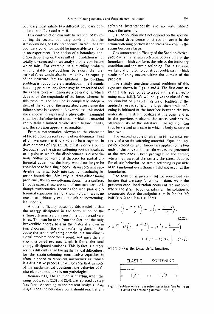
It was first hoped. although in retrospect little practical evidence existed for this optimism. that in dynamic problems, strain softening would not be as troublesome because the inertia of the continuum would alleviate the instability. Support for this can be found in the snapthrough of an arch; in this prob- lem the load-detlection curve contains a limit point after which the force-deflection curve is negative. or softens. A static solution for the snapthrough is often very difficult. whereas a dynamic solution is relatively straightforward because the inertia of the structure alleviates some of the difficulties intro- duced by the negative slope in the force-detlection relation. The use of strain-softening models has be- come quite commonplace in dynamic concrete an- alysis. For example, in Marchertas cut tr/.[3]. strain softening appeared to reproduce the salient features of dynamic response of a concrete reactor vessel even after severe failure had developed. In the com-
munity as a whole. a certain complacency evolved and except for the work of Baiant and colleagues[l,
11. little effort was devoted to examining the basic soundness of numerical solutions with strain-soft- ening materials.
Attention was recently focused on the validity of strain-softening models by the work of Sandier and Wright[4]: they asserted that strain-softening models are basically ill posed because a small dif- ference in load results in large changes in the re- sponse. Sandler’s example. which will be described in more detail later, consists of a one-dimensional rod with the velocity prescribed at one end in which the material strain softens. By increasing the load slightly, a significantly different response was ob- tained for the problem. Sandler and Wright also noted a strong dependence of the solution on the mesh size. They concluded that “a rate-indepen- dent dynamic continuum representation of strain softening is incapable of reproducing softening be- havior in a dynamic simulation of experiments” and then proceeded to show that in this problem the introduction of viscosity eliminates the sensitivity of the response to the load. Incidentally. as will be shown later in this paper, viscous damping is not a panacea for the sensitivity observed in strain-soft- ening solutions: in certain problems which will be described herein. sensitivity to mesh size persists even after the introduction of damping.
In an effort to develop a problem with strain soft- ening in which the localization does not occur on the boundary, we investigated two problems: one, which was presented in Ref. [S]. consists of a linear elastic barjoined to a strain-softening bar. Solutions for this bar were obtained by the method of images and compared to finite-element solutions. These re- sults exhibited convergence with decreasing ele- ment length. BaZant and Belytschko[61 constructed a more interesting problem in which tensile waves are initiated at two ends of a bar so that strain soft- ening occurs at the center. It was shown that a so-

lution to this problem exists but that the behavior
of the strain-softening domain is rather unusual: the
strain softening localizes to an infinitely thin do-
main. a set of measure zero. in u hich the strain
becomes instantaneously infinite and in which the
energy dissipation is zero.
In order to remedy some of these undesirable
features of strain-softening solutions. Baiant. Be-
Ivtschko. and co-workers[7.8] proposed a new non-
local formulation for treating strain softening. Non-
local theories have been introduced by Kroner[9].
Krumhansl[ IO] and Kunin[ I I], and developed fur-
ther by Eringen and co-workers[l?-l-l] and Ede-
len]lS]. The basic ingredient of a nonlocal theory
is that the stress-strain relation is not considered to
be local but relates the stress at an)- point to the
state of deformation within a finite volume about
that point. In this respect. the theory lends itself
admirably to problems of heterogeneous media.
where the representation of the microscopic detail
of strain fields and cracks is an insurmountable
task. By dealing with an average of the strain over
a finite domain about each point. the heterogeneity
can be neglected. and the dispersion which occurs
in inhomogeneous materials can be modeled vvith-
out any artifices. It should be noted that in the tran-
sition from a microstructural theory to a macro-
theory. strains and stresses are often averaged
over finite volumes. Hovvever. this averaging is
only considered in tl~~~~/r~pi/rp the macroconstitutive
equation. In the solution of the governing equa-
tions. the constitutive equations are considered to
apply only to points so the theory is local and the
localization limiting property of nonlocal theories,
i.e. the attribute of the theory which prevents lo-
calization to a set of measure zero. is then lost and
the energy dissipation associated with strain soft-
ening vanishes.
An obvious question which arises is why one
would want to introduce this complication in order
to deal with strain softening. The reason for this is
that when the constitutive equations are applied lo-
cally at points. then. as will be described here. no
dissipation of energy occurs in the strain-softening
domain because it is a set of measure zero. Thus
the material can fail without any permanent dissi-
pation of energy. which is physically quite unreal-
istic. By introducing a nonlocal character into the
constitutive law. it is possible to restrict the local-
ization to a domain of finite size just as is observed
experimentally. and to achieve a finite amount of
energy dissipation in the strain-softening domain.
However. we found we could not simply estend
the existing nonlocal models to account for strain
softeningl7. 161. The existing nonlocal laws are not
even self-adjoint. so they did not lead to symmetric
stiffness matrices. This lack ofsymmetry~ was found
to be undesirable and was corrected by introducing
the same averaging operation over the stresses as
that for the strains. Such double averaging is in fact
required by a consistent application of the v,aria-
tional principls[8]. It was ;dso found that the strxin
softening could only be introduced in the nonlocal
law in a subtle t’dshion. necessitating a split of the
constitutive equation into 2 local and nonlocal 12~.
w.ith the strain softening included only, in the non-
local portion. Numerical experiments indicated that
without this particular combination. numerical ho-
lutions were often unstable.
The nonlocal law as introduced in Kct’s. 17. 81
offers substantial promise in pro\ iding well-posed
solutions for heterogeneous materials that are sub-
jected to damage and hence strain softening. There
are hovvever. substantial breakthroughs that yet
need to be achieved: (1) efficient implementations
of nonlocal laws in the finite-element method: t2)
design of experimental methods for identifying the
local and nonlocal portions of constitutivc laws:
and (3) methods for reconciling the bifurcation be-
tween local damage. i.e. microcracking. and large-
scale fracture of a cleavage type in heterogeneous
materials. However. the work reported here has
shed light on the questions of numerical modeling
of structures in the failure regime when strain soft-
ening takes place and provides the basis for future
work.
We have organized the material as follows: in
Sec. 2 we describe several of the generic onc-di-
mensional problems which can be used to examine
the mathematical character of dynamic strain-soft-
ening solutions. In Sec. 3, the nonlocal continuum
law will be described. In Sec. 4. some finite-element
solutions are presented for planar problems that in-
dicate that the solutions converge to the analytic
solution: however. only for a nonlocal law can finite
energy dissipation be achieved in a strain-softening
domain. In Sec. 5. local and nonlocal solutions will
be given for the converging spherical and cylindri-
cal wave. followed by conclusions in Sec. 6.
The problem by Sandier and Wright[4] is shown
in Fig. I. The essence of their argument was that
the solutions are very sensitive to the constant qi.
which represents the maximum prescribed velocity
at the left-hand boundary. and that the solution
changes markedly and so does not appear to con-
verge as the mesh is refined. Although the Sandkr-
Wright stress-strain law is nice from the viewpoint
“0 w 1-x

that it provid2s a continuous relationship between stress and strain in the loading domain. it is not amenable to any attempts at a closed form solution by d’.Ilembert mzthods because of the dispersive charactsr of the wave solution even in the loading range. For this r2ason. w2 have limited our studies to piecewise linear prescribed velocities or stresses and stress-strain laws of the type shown in Fig. 2: this will be called th2 modified Sandler-Wright problem. Note that the stress goes to zero as the strain becomes large on the strain-softening sides of the law tusually~ the tensile side).
The analytical solutions to this problem are de- velop2d next. The salient characteristic of the ana- lytical solution is the appearance ofan infinite strain on the boundary once the strain E,, is exceeded. The construction of the solution for this case will follow the approach presented by Bafant and Be- lytschko]6] for a similar problem. As will be seen. when strain softening occurs. then the strain im- mediatrly localizes and reaches infinity within a time interval that approaches zero. Therefore. the solution can be generated by adding an image wave which cancels the incident wave so that the strain- softening point is instantaneously converted to a free boundary.
The governing equations can be stated as fol- lows:
0.8 = pi/.,,. (‘.I)
rJ.r = E(E)//.,, = E(Ek.,. (7.‘) - -
where u and E are the stress and strain. II the dis- placement. and subscripts preceded by commas denote differentiation: P is the density and E the tangent modulus. We will consider two types of boundary conditions on the left-hand side, .r = 0:
velocity condition: I/.,(0. 1) = -V,,(1). (2.3)
traction condition: ato. t) = U,)(f). (2.4)
where (f) designates fH(f). H being the Heaviside step function. The velocity boundary condition will be considered first. The right-hand boundary is as-
Fig. 2. Stress-strain law nith strain softening showing no- menclature.
sumed to be sufficiently far so that the rod can be considered semi-infinite.
Not2 that prior to the onset of strain softening. the problem is governed by the standard one-di- mensional vvave equation
I II.,, = 7 II.,,. 12.5)
c’-
where
(2 = t‘ P .
(2.6)
Once the strain-softening regime of the material is attained. then at those points the governing equa- tion is
_T
(‘- II.,, + II.,, = 0. (2.7)
E (-2 = _ -
P (2.8)
and T: vanishes once E,, is attained. Equation (2.7) is elliptic in space-time, which is peculiar in that information can be transmitted at infinite speeds. Hadamard[ 171 commented on this in 1903 and he claimed that the negative character of the square of the wave speed precluded its applicability to real materials since the wave speed would then be im- aginary. However, the case of c = 0 has been treated extensively by Taylor[l8], who noted that for perfectly plastic solids the deformation is lo- calized at the point of impact. Wu and Freund[l9] have recently presented a lucid description of these localization phenomena and investigated the effects of strain-rat2 sensitivity and heat transfer on the localization. However. the analyses were limited to the case where in the limit c = 7 = 0.
We will here consider the strain-softening situ- ation using the concepts developed in 161. The present situation differs from [6] in that the stress wave is a ramp rather than a step wave. but it will be found that all of the singularities associated with a step input remain.
The procedure of constructing a solution con- sists of three steps:
(I)
12)
(3)
It is shown that the boundary between the strain-softening and elastic domain cannot move, so the strain-softening domain is limited to a point. This is shown to imply that the strain and strain rate in the strain-softening points must be in- finite. Since the strain rate is infinite for the class of materials considered here. in which u - 0 as E - x. the stress can be considered to vanish instantaneously at the points which strain soften.
The last conclusion enables the solution to be easily constructed by the d’Alembert method by

simply adding a wave to satisfy the zero stress con- the displacements and stress conditions across the
dition. interface. From eqn (2. IJal. it follows that
For the prescribed velocity problem. let I, be the
time when the left-hand end. .V = 0. reaches E,, and
begin5 to strain soften: I, is given by
it0 e- = z = (itI - f,) f E,,. (2.17,
If the two displacement solutions. eqns (2.1-k)
and Q.15). are now matched across the interface
.Y = s. then
hi,, I, = -
i’,l
and the solution prior to the onset ofstrain softening
is given b),
Strain softening first occurs at .V = 0. We now
show that the boL]nd~tr~ between the elastic and the
softening interface cannot move. For this purpose.
the usual formula for velocity V ot’ discontinuities
is used tn development is given in [6l):
U- - <r- = p L%* - EC). (2.1’)
where the superscripts + and - designate the state
variables to the right and left of the discontinuity,
respectively. If the material is strain softening be-
hind the interface and not yet before it, it follows
that E- > E- and u* 2 CT-. Substituting these in-
equalities into eqn (2.12). it follows that V’ must be
negative or zero: since the former assumpt;on
would yield an imaginary velocity for the discon-
tinuity. only V = 0 is tenable. and it can already
be concluded that
ir* = CT-. (2.13)
To show that the strain and strain rates must be
infinite at a point which strain softens. a solution
is constructed in the strain-softening domain which
is considered to be U 4 A G s where .s - 0. It can
be seen that
,,* = - y ((,, - $) (2.14b)
satisfies the governing equation in the strain-soft-
ening domain. 12.7). This solution. t2.14). is now
matched to a solution in the elastic domain
where the second term is a wave emanating in the
strain-softening region w,hich w?ll be used to match
II” + It/( f - II ) + E,,j.T
= - T ((t - $) f f(E). i7.i&l)
(2.18b)
Eliminating (I from eqns (7.17) and 12.18) yields
It can be seen that ass-+ 0. E- -+ 0 instantaneously.
which through eqn (2.13) implies uc = 0. The func-
tion f(Q is then found from this condition. Using
the displacement field of eqn f2.15) and letting tr+.
and hence E + , vanish. we find
f’(~, = E,,L’ H (1 - I, - ;)
f LI~(~ - ti - $, (2.20af
f(S) = E,‘(’ (r - II - ;>
Hence the complete solution is
This solution will subsequently be compared to fi-
nite-element solutions.
The solution for the stress boundary condition.
eqn (2.4). can be found by replacing z’(, by u,,ciE.
However. in the prescribed stress form of this prob-
lem. eqn (7.4). the introduction of the image at the
strain-softening point poses a difficulty since the
first point to strain soften is initially on the bound-
ary. Thus. in one sense it can be said that this
Strain-softening material5 and finite-element wIution4 167
boundary must satisfy two different boundary con- softening instantaneously and no wave should
ditions: eqn (3.4) and cr = 0. reach the interior.
This contradiction can only be reconciled by re-
quiring the second boundary condition (that the stress vanishes) to take precedence. In fact. the first boundary condition would be impossible to enforce in an experiment. The notion of a boundary con- dition depending on the result of the solution is not totally unexpected in an analysis of a continuum which fails. For example. in a buckling problem with unstable postbuckling behavior, the pre- scribed force would also be limited by the capacity of the structure. Yet the situation in the buckling problem is not completely analogous: in a dynamic buckling problem. any force may be prescribed and the excess force will generate accelerations. which depend on the magnitude of the force, whereas in this problem, the solution is completely indepen- dent of the value of the prescribed stress once the failure stress is exceeded. Nevertheless, this model does appear to represent a physically meaningful situation: the behavior of a rod in which the material can sustain a limited tensile strain before it fails,
and the solution appears reasonable.
(2) The solution does not depend on the specific functional dependence of stress on strain in the strain-softening portion if the stress vanishes as the strain becomes large.
One conceptual difficulty of the Sandler-Wright problem is that strain softening occurs only at the boundary, which confuses the role of the boundary condition and the strain softening. For this reason we have attempted to construct problems in which strain softening occurs within the domain of the problem.
From a mathematical viewpoint, the character
of the solution presents some other dilemmas. First of all, we consider 0 < x < s to be a segment in developments of eqn (2.19), but it is only a point. Second, since the strain softening portion localizes to a point at which the displacement is discontin- uous, within conventional theories for partial dif- ferential equations, the body would no longer be considered to be a single body: strain softening sub- divides the initial body into two by introducing in- terior boundaries. Similarly in three-dimensional problems, the strain-softening domain is a surface. In both cases, these are sets of measure zero. Al- though mathematical theories for such partial dif- ferential equations are not known to us, there is no reason to arbitrarily exclude such phenomenolog- ical models.
The strictly one-dimensional problems of this type are shown in Figs. 3 and 4. The first consists of an elastic rod joined to a rod with a strain-soft- ening material[S]. We will not give the closed form solution but only explain its major features. If the applied stress is sufficiently large. then strain soft- ening is initiated at the interface between the two materials. The strain localizes at this point. and as in the previous problem. the stress vanishes in- stantaneously at the interface. The solution can thus be viewed as a case in which a body separates into two.
The second problem, given in (61. consists en- tirely of a strain-softening material. Equal and op- posite velocities I’,) (or forces) are applied to the two ends of the bar. so that tensile waves are generated at the two ends. These propagate to the center; when they meet at the center. the stress doubles for elastic behavior, so strain softening is possible at this midpoint even though it did not occur at the boundaries.
The solution is given in [6] for prescribed ve- locities that are step functions in time. As in the previous case, localization occurs at the midpoint where the strain becomes infinite. The solution is symmetric about the midpoint x = 0; for the left half (x < 0 and 0 C t c 2Llc)
Another difficulty posed by this model is that the energy dissipated in the formulation of the strain-softening region is not finite but instead van- ishes. This can be seen from the fact that the only irreversible energy loss in the material shown in Fig. 2 occurs in the strain-softening domain. Be- cause the strain-softening domain in a one-dimen- sional problem becomes a point, and since the en- ergy dissipated per unit length is finite, the total energy dissipated vanishes. This in fact is a more serious difficulty than the mathematical difficulties, for the strain-softening constitutive equation is often intended to represent microcracking. which is a dissipative process. It will be seen that, in spite of the mathematical questions, the behavior of fi- nite-element solutions is not pathological.
II = Ll,,(f - +> - <!,,(, - +).
(2.22a)
+ 4 (et - I!,) 6(r) , (2.22b) 1 where 6(x) is the Dirac delta function.
Remarks: (1) The solution is puzzling when the ramp loads, eqns (2.3) and (2.4). are replaced by step functions. According to the present analysis, if u,,
> E,,E, then the boundary point should reach strain
ELASTIC SOFTENING
-L/2
Fig. 3. Problem with strain softening at interface between elastic and softening domain (Ref. [.(]I.

“0 I V, bX
I------+-----A Fig. 1. One-dimensional problem in uhich strain wtiening
occurs at v = 0 (Ref. 161).
Fig. 5. Spherical converging wave problem
Another problem we have considered is a sphere
loaded on its exterior surface (see Fig. 0. This
problem is not easily physically realizable with a
tensile load: however. it is physically meaningful
with a compressive load, and strain softening can
occur in some materials in compression (although
the stress usually will not vanish as the dilatation
becomes large).
This problem has an intriguing feature. Consider
a load which is a ramp function in time. Prior to the
onset of strain softening at an interior surface, part
of the wave can have passed through this surface.
Since the stresses in the wave which are inside the
initial surface of strain softening are amplified as
the wave passes to the center. the formation of ad-
ditional strain-softening surfaces is possible. As a
result. this problem has considerably more struc-
ture than the one-dimensional problems.
3. NONLOCAL CONTINLWI FOR STRAIN SO+TENISG
The major shortcoming of strain-softening
models for representing local damage is that the lo-
calization phenomenon associated with strain soft-
ening results in no dissipation of energy. For ex-
ample, in one-dimensional problems. the strain-
softening process is limited to a single point and
since the rate of work per unit length is finite, the
amount of work dissipated in the strain-softening
domain vanishes. Analogously. in three-dimen-
sional problems, strain softening localizes to a sur-
face. and since the work per unit volume is again
finite. the total energy dissipation due to the sep-
aration across the surface is finite. Thus. no energy
is required to separate the material along the surface
of strain softening, which is physically quite un-
realistic. It should be stressed that all of these com-
ments apply only to materials in which the stress
across the surface tend\ to zero ;IS the strain be-
comes large: if the stress tends to some nonzrro
value. then the response of the material may be
quite different and the dissipation no longer van-
ishes. However, any dissipation in excess of that
which corresponds to the perfectly. plastic dissi-
pation associated with the final stress vanishes.
To achieve finite energy dissipation during fail-
ure by strain softening. the artifice of imposing ;I
certain minimum element size which depends on
the aggregate size (crack band model) has been pro-
posed[Z]. However, this artifice may be inconven-
ient in practical analysis. since it requires the ele-
ment size to be dictated by a material constant
rather than by the size of the structure.
In order to avoid this difficulty. we have inves-
tigated the possibility of using nonlocal constitutive
laws in which the stress at a point is related to the
weighted average of the strain in a neighborhood ot
that point. This is a special case of the existing
(or classical) nonlocal continuum theories[%-14).
However, it was found to be necessary to make two
modifications of this theory in order to obtain re-
alistic results in the strain-softening regime: ( I) the
existing nonlocal theory is not self-adjoint and
hence possesses certain spurious zero-energy
modes of deformation: (2) in order to achieve stable
solutions even in one dimension in the presence of
strain softening with a constant weight. ;I material
law consisting of a combination of a local law vrith-
out strain softening and a nonlocal law with strain
softening was required.
We will now sketch the essential features of this
nonlocal theory for one-dimensional problems. De-
tails may be found in Refs. 17. 81. The fundamental
assumption in a nonlocal theory is that the nonlocal
strain r at a point is a weighted average of the strains
in a neighborhood of that point. Thus
i
t-12
E(s) = ct.\’ + .S)II’l.S) d.s t-12 (3. I)
-I -I 2 i),,
= J , _, ~ z (x + .S)~l~(.S) d.s.
where n’(.s) is a given weighting function. The
stress-strain law is then written in terms of Z. and
its rate form is
u.,(x) = L-(E)E.,lx). (3.2)
Although the classical nonlocal theory directly
uses the stress CT in the momentum equation. eqn
(2. I ). the resulting form is not self-adjoint[ In]. This
leads to the existence of spurious. zero-energy’
modes of deformation for certain weighting func-
tions II.(.V): deformations which are associated with
vanishing strains E and hence do not generate any’
stresses. These spurious modes have been found fc71
uniform (constant) weighting functions 1i.t~).
To remedy this difficulty. the stress 17 is pro-

Strain-\oftenlng material\ and finite-element wlurion~
cessed through an operator identical to (3.1).
I
I -/I i3.r) = a(.r + .s)u~(.v) ds. (3.3)
t-12
and the resulting stress is used in the equation of
motion. eqn (2.1). Once eqn (3.3) is added to the
system. spurious modes are eliminated even for
constant weighting functions nG). It was also
shown by Bafant[S] that the averaging of a(x) is
required within a consistent application of a vari-
ational principle such as the principle of virtual
work. A nonlocal continuum which is characterized
by double averaging. once on the strains. as in 0. I) and then on the stresses. as in (3.3). is the limiting
case of a series of imbricated (overlapping) finite
elements. Therefore. this type of nonlocal contin-
uum was termed an imbricated continuum by Ba-
iant[8].
Even with a self-adjoint form of the nonlocal
laws. solutions for strain-softening materials are un-
stable for constant weights ~cG). So far, only by combining a local and nonlocal law has stability
been achieved[l6, 71. By superimposing two dis-
tinct field systems, one local and wirhour strain soft-
ening. and a nonlocal law ~vith strain softening,
stability is achieved in a model which exhibits a
negative slope for a finite segment.
The governing equations for this model can be summarized as follows:
o.r = EC., Ecan be negative, (3.4)
T., = EE,~, E>O. (3.5)
eqn (3.3): u--+ ij’, (3.6)
S=Cl -y)cJ+yT, O<y<l. (3.7)
5-C = Pll.rr. (3.8)
Finite element solutions for this nonlocal law are given in Sec. 5 for cylindrical and spherical geo-
metries. These results were obtained with an im- bricate finite-element model, and with various fi- nite-element meshes. It will be seen that the strain distributions computed by the nonlocal law are quite well-behaved for various meshes, whereas the local formulation predicts strain that vary errati- cally with mesh refinement.
1. FISITE-EI.EMENT SOLUTIONS FOR PLA\NAR
PROBLE\lS
Finite-element solutions for the moditied San-
dler-Wright problem. Fig. I, obtained with the
local material law given in Fig. 2. are shown in Fig.
6. Solutions were obtained with meshes of 50. 100.
and 200 elements. Linear displacement. constant
strain elements. and lumped mass matrices were
used. Time integration was performed with the cen-
tral difference method.
g -3.700
0 -e- AN.4 soi
-6.700 + 100 ELE
- 10.000 ,000 2.000 4.000 6.000 8.000 10.000
TIME - SEC (xl O-‘)
Fig. 6. Velocity-time history at .v = L/4 for geometry shown in Fig. I. stress-strain law given in Fig. 2: t,, =
O.OI. E, = 0.05. L = 100. C‘ = IO’.
The finite-element solutions are compared with
the analytic solution given in the Sec. 2. It can be
seen that the agreement is quite good and improves
with mesh refinement. although the instantaneous
drop in the velocity. which is a result of the strain
localization, cannot be reproduced even with the
finest mesh.
The rate of convergence for the case when E, =
er = 0.01 is shown in Fig. 7. Here the error (3 is
defined by
- I,‘~,‘)’ d.v dt. (4. I)
where v with superscripts FEM and ANA are the
finite-element and analytic velocities. respectively.
As can be seen from Fig. 7. the rate of convergence
is approximately proportional to I/‘.‘” where 11 is the
element length. This is not much less than the the-
ij
( (i=&
I i
In h 1
1
1 Fig. 7. Rate of convergence of finite-element solution for velocity to analytic solution for modified Sandier-Wright
problem with e, = e, = 0.01.

TED BELYTKHKOC~ trl
i0 -1.900 -1.450 -1.000 - 550
In h
Fig. 8. Rate of convergence of finite-element solution for velocity to analytic solution for modified Sandler-Wright
problem with t, = ZEN = 0.02.
-.lLm I=--- & -.900
s Y
-1.700 I
*so0 i ma 2.cal 4.m 6.000 8.000 10.000
TIME - SEC (x10-')
- AhA SOL
-a- 50 ELE
+3- 100 ELE
Fig. 9. Finite-element solution to modified Sandler- Wright problem with p = p,,H(f). H being the Heaviside
step function.
oretical value of 11’ expected for linear solutions by
these methods, so the sensitivity to meshing which
Sandier and Wright pointed out is not evident. The
rate of convergence for a material with E, = Ze,. =
0.02 is shown in Fig. 8; as E( increases, the rate of
convergence deteriorates. Figure 9 shows the finite-
element solution when the input is a step function.
Theoretically. there should be no waves inside the
rod. but because of the finite size of the elements.
a small pulse penetrates the mesh in a numerical
solution.
5. FINITE-ELEMENT SOLUTIONS FOR SPHERICAL AND CYLINDRICAL PROBLEMS
As mentioned in Sec. 2. the converging spherical
wave problem is particularly intriguing because it
offers the possibility of strain softening being ini-
tiated at many points by a wave. Although we have
not been able to find a closed form solution for this
problem. we have examined both local and nonlocal
finite-element solutions. The local finite-element
solutions exhibit radical differences as the mesh is
refined. and this ostensible absence of convergence
is not alleviated by the addition of damping. Non-
local solutions are free of these difficulties. These
solutions will be summarized in this section.
In spherical or cylindrical coordinates. the
strain-displacement relations are
Ex=u,,, c,=;, t; = l y (spherical),
eL = 0 (cylindrical), (5.1)
E = E, + 3,. PI = i (E, - E,).
e, = 6 (E, - E,) (spherical). (5.2)
E = E, + 2EV, (‘, = i (ZE, - E, ).
e,. = i (EV - E,) (cylindrical). (5.3)
We denote by F,. E,.. E. 7,. 7,. the means of e,.
ey. e, e,, e,, respectively; defined as in eqn (3.1).
The stress-strain law is
o.r.1 = i& + z?Z,,,,
o,., = KE., f 2?%,.,,.
79.1 = KE,, + ZGr,,,,
‘Tb .I = KE.~ + ZGr,,,.
and the total stress S is obtained by
1 .I * /:2
v, Lr) = a,(~ + S)II~S) ds. r_,,?
s,, = (1 - y)Z, + yir,
s,. = (I - y)aV + -yTY.
The equation of motion is
s,,., + f (5, - S,.) = PlJ.,, (spherical),
(5.4)
(5.5)
(5.6)
(5.7)
ST., + ; (S, - S,.) = ptt,,, (cylindrical). (5.8)
Here u = radial displacement (Fig. 10~): e.<, E, =
radial and circumferential normal strains (local): E
= volumetric strain; e,. e,. = deviatoric strains
(local): T.,, TV = local radial and circumferential nor-
mal stresses: o.,, u,. = broad-range radial and cir-
cumferential normal stresses: S,, S,. = total radial -- and circumferential normal stresses: K. G. K, G = local and broad-range (nonlocal) bulk and shear
moduli. In eqns (5.4) and (5.5) isotropy of the ma-
terial is assumed. The shear moduli G and c are
assumed to be constant. while K and ?? depend on
Strain-softening materials and finite-element solulions lil
b) used: bulk modulus K = I .O. density p = I. shear modulus G = I x IOwh. eV = 1.0. e, = 5.0 (see
bottom of Fig. I I ). Damping was added by a viscous
stress defined by
d) local
-%,\I1 - _ -- _.. e-7:
-al nonlocal ;-l i itl -
I
r--
Fig. IO. Notation for spherical and cylindrical wave prob- lems.
E and Z, respectively: K > 0 but ?? may become negative, which represents strain softening.
We consider waves generated by a sudden ap- plication of a uniform normal traction at the exterior surface of a hollow sphere or a hollow infinite cyl- inder. The traction is a Heaviside step function of time. so the boundary condition at .r = h (Fig. IOa) is u., = p. H(r), and the interior surface is load- free, i.e. ux = 0 at x = o (a, h = internal and external surface radii). Initially, the body is at rest. The elastic solution[20], consists of a step wave with a strain which grows as the wave propagates toward the center.
The closed form solution is
for 7 2 0, (5.9)
as may be checked by substitution in eqns (5. I )- (5.8) with y = I. K = constant; 7 = t - (h - v)/
c,, 5 = 2 cj/(bC,), w = .$+z)’ - I I”‘, (‘, = [3K( I
- u)/(l + u) p]“‘, cz = (G/p)“‘, v = (3K - 2G)/
(6K + 2G) = Poisson’s ratio.
For the numerical solutions, one-dimensional meshes with (Fig. lob) two-node elements with lin- ear displacements and a single quadrature point (at the element center) were used. The local elements are of length /I and the imbricate elements of length I = n/r. The mass matrix is lumped.
The first group of numerical solutions was made with the aim of examining the character of the spherical wave solution and determining whether damping is sufficient to achieve well posedness, as in the planar one-dimensional problem[4].
Shear moduli G and ?? are assumed to be neg- ligibly small (IO-‘). The following constants were
g;;‘ = 21 (pK)’ ’ E8,,. (5.10)
with n = 0. I. This provided enough viscosity to damp the cutoff frequency of the mesh by 44% and 6% of critical damping in the fine and coarse meshes, respectively. In some solutions. the damp- ing was turned off whenever er, the strain at which the stress vanishes. was reached. This is called a
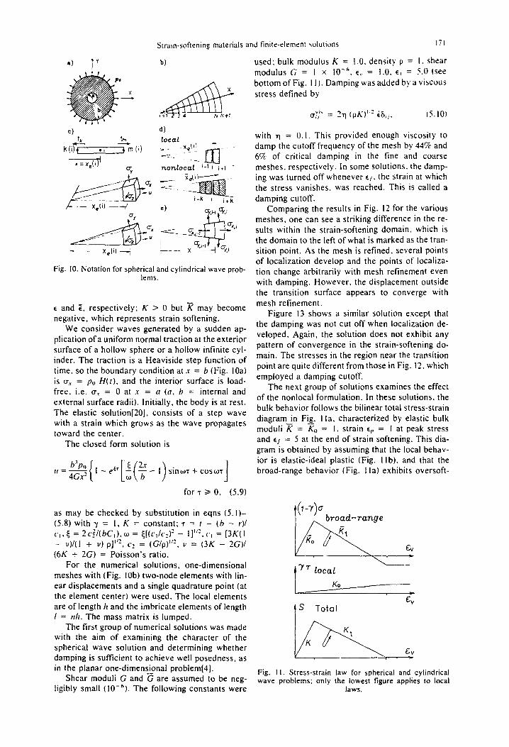
damping cutoff. Comparing the results in Fig. I2 for the various
meshes, one can see a striking difference in the re- sults within the strain-softening domain. which is the domain to the left of what is marked as the tran- sition point. As the mesh is refined, several points of localization develop and the points of localiza- tion change arbitrarily with mesh refinement even with damping. However, the displacement outside the transition surface appears to converge with mesh refinement.
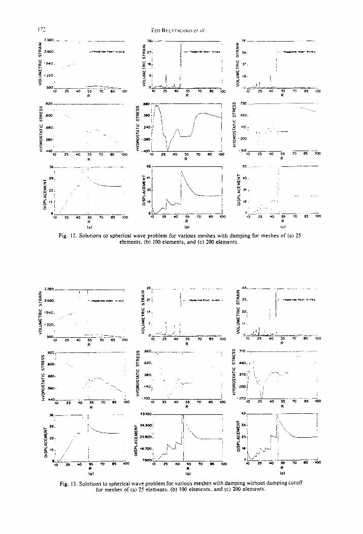
Figure I3 shows a similar solution except that the damping was not cut off when localization de- veloped. Again, the solution does not exhibit any pattern of convergence in the strain-softening do- main. The stresses in the region near the transition point are quite different from those in Fig. 12, which employed a damping cutoff.
The next group of solutions examines the effect of the nonlocal formulation. In these solutions. the bulk behavior follows the bilinear total stress-strain diagram in Fig. I la, characterized by elastic bulk moduli K = K,, = I. strain E,, = I at peak stress and er = 5 at the end of strain softening. This dia- gram is obtained by assuming that the local behav- ior is elastic-ideal plastic (Fig. I lb), and that the
broad-range behavior (Fig. I la) exhibits oversoft-
6”
t s Total
Fig. I I. Stress-strain law for spherical and cylindrical wave problems: only the lowest figure applies to local
laws.
DIS
PL
AC
EM
EN
?
DIS
PL
AC
EM
EN
T
HY
MIO
STA
TIC
S
TR
ES
S
HY
DR
OS
TA
TIC
S
TR
ES
S
VO
LUM
ETR
IC
STR
AIN
VO
LUM
ETR
IC
STR
AIN
5 ‘I!
“m
,.
__
-i---
1
5 j
e”
f j
.‘
I
3 I
HY
DR
OS
TA
TIC
S
TR
ES
S
VO
LUM
ETR
IC
STR
AIN
DIS
PL
AC
EM
EN
T
DIS
PL
AC
EM
EN
T
HY
DR
OS
TA
TIC
S
TR
ES
S
HY
DR
OS
TA
TIC
S
TR
ES
S
VO
LUM
ETR
IC
STR
AIN
VO
LUM
ETR
IC
STR
AIN
F
2
Strain-Softening mLlterials and finite-element solutions 173
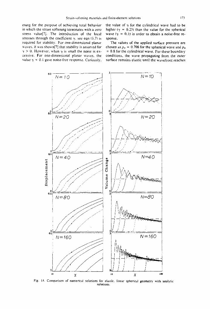
wing for the purpose of achieving total behavior in which the strain softening terminates with a zero stress value[?j. The introduction of the local stresses through the coefficient y. see eqn (3.7) is required for stability. For one-dimensional planar bvaves. it was shown[7] that stability is assurred for y > 0. However. when y is small the noise is ex- cessive. For one-dimensional planar waves. the value y = 0.1 gave noise-free response. Curiously.
6X
600 r
N=20 I(’ ,(’ _._-
jll_
// _*,* A ,,** /’ ,,’ .._’ .:’ / ’ _, I’ ,.:
/ / , ,’ ,.I’-
/ ’ I’ ._I’ ,/ ,//I /* _:”
,.,’
_ / _ _** _/” _-_.-.
the value of y for the cylindrical wave had to be higher ty = 0.3) than the value for the spherical
wave (y = 0. I) in order to obtain a noise-free re-
sponse. The values of the applied surface pressure are
chosen as p. = 0.708 for the spherical wave and p,, = 0.8 for the cylindrical wave. For these boundary conditions, the wave propagating from the outer surface remains elastic until the wavefront reaches
0 iv=40 M
ol’ J J !
Fig. 14. Comparison of numerical solutions for elastic. linear spherical geometry with analytic solutions.

30% of the thickness h - (I. The dimensions are (I = 10. h = 100. L = h - (I = 90.
In order to ascertain the mesh refinement nec- essary for this class of problems. elastic local so- lutions were obtained first. The convergence with
a-
t
i 0 ’ 3 r I I
: k r N=40
increasing numbers of elements (ic’ = IO. 20. 40. 80. 160) is shown in Figs. I-l and 15. The results converge to the exact solution given by eqn (5.9).
Subsequently, the problem was solved for a non- local continuum (E, = I. E j = 5) with characteristic
“y------ 1 1 N=10
I
-1 N=20
N=40
,/; i 1,
/ ; /\ )/ ,‘d’ i’ ii-,
Fig. 15. Numerical solutions for elastic, linear cylindrical geometry.
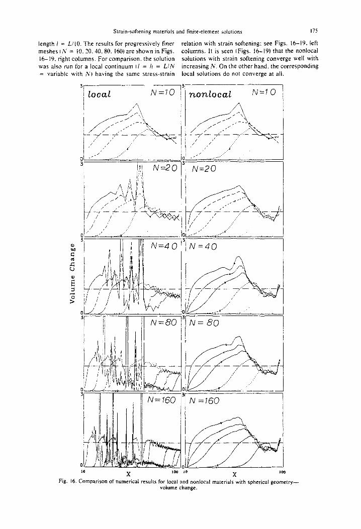
Strain-softening materials and finite-element solutions 175
length 1 = L/IO. The results for progressively finer relation with strain softening: see Figs. 16-19. left
meshes IN = IO. 20.10.80. 160) are shown in Figs, columns. It is seen (Figs. 16-19) that the nonlocal
16- 19. right columns. For comparison. the solution solutions with strain softening converge well with
was also run for a local continuum ii = Ir = L/I%’ increasing N. On the other hand, the corresponding
= variable with A’) having the same stress-strain local solutions do not converge at all.
N=lO
10 X
-_L
Iv=80
N=160
loo 10
N=40
N=80
X loo
Fig. 16. Comparison of numerical results for local and nonlocal materials with spherical geometry- volume change.
local
N-40
nonlocal ____*. / ,’ _-+-_-
N=40 G= /I
/ ,.-. ,___-*
1. _;’ 1:I.;: ,;’
,;’ ,,,’
,,1’ .:’
__=
10 X 100 JO X 10
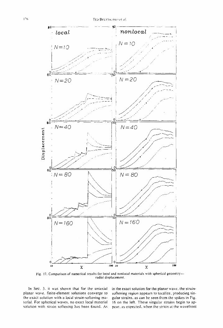
Fig. 17. Comparison of numerical results for local and nonlocal materials with spherical geometry- radial displacement.
In Sec. 3. it was shown that for the uniaxial in the exact solution for the planar wave. the strain-
planar wave, finite-element solutions converge to softening region appears to localize. producing sin-
the exact solution with a local strain-softening ma- gular strains, as can be seen from the spikes in Fig.
terial. For spherical waves. no exact local material I6 on the left. These singular strains begin to ap-
solution with strain softening has been found. As pear. as expected. when the strain at the wavefront

Strain-softening materials and finite-element solutions
IO X
100 10 X too
Fig. 18. Comparison of numerical results for local and nonlocal materials with cylindrical geometry- volume change.
reaches the strain at which strain softening begins. points increases with increasing mesh refinement. In contrast to the planar wave. there is not one point The impression is that of chaos. It is anticipated of localization but many, and they appear at dif- that if the loading is a ramp function in time, the ferent locations for different N [i.e. for different set of localization points would be an infinitely mesh re~nements~. and the number of localization dense set of discrete points. i.e. a Cantor set. The

TED BELYTKHKO ('r ol.
60, ______ __. T
local nonlocal
N = 10 , i:,,’ >,,,’ _/’
/,’ ~
,/: ’
,/: ,/’ I
I i
Jr --G-- *. ..2.
N=20
,’ ,’ ,I ,,/‘, ,’ ;’
;.. ..’
,/ ,a , ,, .Y’
// , >’ .,,I’
*, / ,,,’ _, ; - --.
Fig. 19. Comparison of numerical results for local and nonlocal materials with cylindrical geometry- radial displacement.
Strain-softening materials and finire-element solutions 179
reason for the appearance of multiple strain-soft-
ening points (the spikes in the left columns of Figs.
16 and 18) is that part of the strain step at the wave-
front is transmitted across the surface of strain soft-
ening before the stress is reduced to zero. The part
of the wave which has been transmitted then grows
as the wavefront converges toward the center until
the elastic limit ep is reached again. so the situation
repeats itself.
6. COSCLLWOSS
The following are the major conclusions of the
work:
I. Analytic solutions can be established for cer-
tain simple problems which include strain-softening
materials. The solutions exhibit singular strain dis-
tributions but the rate of convergence of tinite-ele-
ment solutions is quite rapid.
2. In the spherical wave problem, numerical so-
lutions of strain-softening models exhibit severe de-
pendence on element mesh size. This is particularly
true of field variables inside the surface of initial
strain softening. Nonlocal models provide rapidly
converging solutions to this problem.
3. A major difficulty of local laws \vith strain
softening is that the energy dissipation vanishes.
Thus, the failure process is not accompanied by en-
ergy dissipation. which is physically unrealistic.
4. Nonlocal laws provide a means for obtaining
rapid convergence and finite energy dissipation in
failure. However, the technology for efficiently im-
plementing these techniques in large-scale, multi- dimensional problems remains to be developed.
Ack,ro,c,/rd.~fnrnrs-We gratefully acknowledge the sup- port of Air Force AFOSR Grant 83-0009 lo Northwestern University.
1.
2.
3.
4.
5.
6.
REFERENCES
Z. P. Batant and L. Cedolin, Fracture mechanics of reinforced concrete. J. Engng Mech. Div. ASCE 106, 1287-1306 (1980): Discussion and Closure in 108.464- 471 (1982): Z. P. Bafant, Instability, ductility and size effect in strain-softening concrete. J. Engng Mech. Div. ASCE 102, EM2. 331-334 (1976): discussion 103. 357-358. 775-777 (1977); 104,‘501-502 (1978). S. H. Marchertas, S. H. Fistedis, Z. P. Barant, and T. Belytschko, Analysis and application of pre- stressed concrete reactor vessels for LMFBR con- tainment. Nucl. Engng Des. 49, 155-174 (1978). I. Sandier and J. Wright, Summary of strain-softening. In Theoretical Foundations for Large-Scale Compu- tations ofNonlinearMateria1 Behavior, DARPA-NSF Workshop (Edited by S. Nemat-Nasser). Korthwest- em University (1984). T. Belytschko, Discussion of I. Sandier in Theoretical Foundations for Large-Scale Computations of Non- linear Material Behavior, DARPA-NSF Workshop (Edited by S. Nemat-Nasser), pp. 285-315. North- western University (1984).
Ntrmrricrrl rrlgorithm for sphc~ricul an~c,vlindricctl NY,~‘~.s
(I) Read (I. h. 1. n. It (time step). N,.. N,.. NI. N,(number of local elements, imbricate elements. nodes, and time steps, respectively), y. and po. Generate arrays l(i). k(i).
I,(i). x,.(i). I(i). Z(i). i,.(i), T,.(i) giving the number of the left and right nodes of the ith local or imbricate element, its length. and its coordinate at the center ofelement. Also generate externally applied nodal forces ft.::. Initialize as zero the values (for r = I) of ill. kI. ;rl. T,~. v,~. max Q. max fl. T,,.~ *.A. urn.,< c.l forall k = I. . . N,. (local
Z. P. Bafant and T. B. Belytschko, Wave Propagation in Strain-Softenine Bar: Exact Solution. Retort No.
elements) and k = I. . Iv,. (imbricate elements). (2) DO 8. r = 2. . N,. (3) Initialize nodal forces FL = 0. fl = 0 (for all nodes, !i = I. , Nk). (4) DO 5 i =_ I. , N,. (local elements). (5) Set k = k(i), m = G(i). x = x,.(i) and evaluate 1c,i = (v.,, - I%)~frill. E,, 6 E,, + AE,, AE,, = l&,, + 1’1) ~rtl2.r. Ed, +-r,.; + SE,.. For spherical wave l\e, = AC,, + XE,~. and for cylindrical wave AC, +- AE,, + 16,;: e, + ei + ALL;. Then call a subroutine which determines the incre- mental (tangential) moduli K,. G, for the local elements from their strainse,,. E,,. E, and also decides whether virgin loading. unloading. or reloading applies. Then calculate
_. AT,, = K; AC, + ZG, e,,. AT,, = Ki 1~; + 2G, e,,. T,~ +
7.
8.
9.
10.
II.
12.
13.
14.
15.
16.
17.
18.
19.
20.
83-lOi401w to DNA. Center for Concrete and Geo- materials, Northwestern University, Evanston, Illi- nois, Oct. 1983. Also, J. Engng .Mech. Div. ASCE, 111, 381-389 (1985). Z. P. Batant. T. B. Belytschko. and T.-P. Chang. Continuum theory for strain softening. 1. Engng
Mech. ASCE 110, 1666-1692 (1984). Z. P. Baiant. Imbricate continuum and its variational derivation. J. EnanP Jfech. ASCE 110. 1593-1712
I I
(1984). E. Kraner, Elasticity theory of materials with long range cohesive forces. Int. J. Solids Srruct. 3, 731-
742 (1967). J. A. Krumhansl. Some Considerations of the Relation Between Solid State Physics and Generalized Contin- uum Mechanics. Mechanics of Generalized Conrinua
(Edited by E. Krbner), pp. 198-31 I. Springer-Verlag, Berlin (1968). I. A. Kunin, The Theory of Elastic LMedia with Mi- crostructure and the Theory of Dislocations. Me- chanics of Generalized Continua (Edited by E. Kriiner), pp. 321-328. Springer-Verlag, Berlin (1968). A. C. Eringen, Nonlocal polar elastic continua. Int. J. Engng Sci. 10, I-16 (1972). A. C. Eringen and D. G. B. Edelen, On nonlocal elas- ticity. Int. J. Engng Sci. 10, 233-248 (1972). A. C. Eringen and N. Ari, Nonlocal stress field at Griffith crack. Cyst. Latt. Def. Amorph. Mat. 10,33- 38 (1983). D. C. B. Edelen. Non-local variational mechanics I- Stationarity conditions with one unknown. Int. J. Engng Sci. 7, 269-285 (1969). Z. P. Barant and T.-P. Chang, Nonlocal Continuum and Strain-Averaging Rules, Report No. 83-I 1/4OIi. Center for Concrete and Geomaterials, Northwestern University, Evanston, Illinois, Nov. 1983; also J. Engng Mech. ASCE (in press). J. Hadamard, Leqons sur la propagation des ondes, Chapt. VI. Hermann et tie, Paris (1903). G. I. Taylor, The testing of materials at high rates of loading. J. Insr. Civ. Engng 26, 486-519 (1946).
F. H. Wu and L. B. Freund, Deformation trapping due to thermoplastic instability in one-dimensional wave propagation. J. Mech. Phys. Solids 32(2), 119- 132 (1984). J. D. Achenbach, Wave Propagation in Elastic Solids. North-Holland, Amsterdam (1973).

IX0 TM BELI.TSC.HKO (21 cd.
78, L A;,,. :,, = T,, - AT,,. Then calculate all the local Then calculate all the nonlocal nodal forces at element nodal forces a[ element nodes /, and VI f Fig. t&c). nodes b and m (Fig. IOd).
= - y [Tc, x2 - T,, (I - ?h)hl.
(spherical)
AFL= --
(Al) (spherical) (MI
AF,,, = + [u.;s’ + u,, (.r + ;j h] . Icylindricall (AZ)
Af,,, = y (T,, .I- + I/r r,,)J. AF& = - + (o,,.r - ; UXi) .
These forces are accumulated at each node, fk + fk +
Af4. f”, +-- fm + Afrn.L (6) DO 7. i 5 I, , E, (imbricate elements). (7) Set k = k(i). m = Xi). I = i,fi). x = f,(i) and evaluate . _._ AZ,; + (v, - vm)Arll. ,i +- ?,i + A&* AZ.“/ - (u, + L’~)A rl2.r. Fyi + Z,; + AZ,., For spherical wave AZ; = A,, + 217,;. and for cylindrical wave Zi = AZ.,, + AZ,+; E = 7; + AZ;. Then call a subroutine w&h determines the incremental (tangential) moduli K,. Gi for the imbricate elements from their mean strains &. Z.Vi, Zi and also de- cides whether virgin loading, unloading, or reloading ap- plies. Then calculate Au,, = Ki AC, + ZGiAeri. Au,; =
z,Aei + ZG,Ae,.i, u.1; + u,, + Au,;. cruj + cr,., + AuO,.~.
(cylindrical) (A4)
I--Y AF, = -
n These forces are then accumulated at each node: FL + FL + AFL. F.,, + Fe,, f AF,,,. (8) DO 8. k = I. . . . NA (all nodes). (9) Calculate 1’~ = r’l + (FL + FL + fC”)~/i(plr.v’). 11~ = ,,I, + l.llV~.
For more detailed explanations. a similar algorithm for planar stress wave given in Ref. 171 may be consulted. It may be checked that the sum of the nodal forces given by eqns (A I )-(A41 on one node yields a second-order discrete approximation of the conrinuum equation of motion (5.X).


