國立成功大學

機械工程學系

碩 士 論 文

貝貝貝氏氏氏更更更新新新法法法應應應用用用於於於皮皮皮帶帶帶系系系統統統與與與不不不確確確定定定性性性壽壽壽命命命資資資料料料之之之設設設計計計整整整合合合

A Bayesian Based Updating Scheme for Belt-Pulley Systems Design

with Censored Life Data

研 究 生： 韓佾君

指導教授：詹魁元博士

中 華 民 國 一 百 零 二 年 六 月

貝氏更新法應用於皮帶系統與不確定性壽命資料之設計整合

A Bayesian Based Updating Scheme for Belt-Pulley Systems Design

with Censored Life Data

研 究 生： 韓佾君 Student: I-Chun Han

指導教授： 詹魁元博士 Advisor: Dr. K.-Y. Chan

國 立 成 功 大 學

機 械 工 程 學 系

碩 士 論 文

A Thesis

Submitted to Department of Mechanical Engineering

National Cheng Kung University

in Partial Fulfillment of the Requirements

for the Degree of

Master of Science

in

Dept. of Mech. Eng.

June 2013

Tainan, Taiwan

中華民國一百零二年六月

貝氏更新法應用於皮帶系統與不確定性壽命資料之設計整合

學生：韓佾君 指導教授： 詹魁元博士

國立成功大學機械工程學系

摘 要

皮帶系統為常見的動力傳輸系統。在此論文中，我們探討量產車輛中的皮帶傳動系統的設

計，設計的主要目標為決定皮帶輪與張力輪的位置，以確保皮帶在靜態與動態行為下的表現

均合乎要求，並考慮老化及不確定因素，使得皮帶系統在整個生命週期內均有良好的表現。

然而，在皮帶設計過程中，仍然有許多困難尚未被解決。皮帶的結構為非均勻的複合材料，

其中包含橡膠、鋼芯線體等。老化與不確定因素會使得皮帶特性難以預測，現有之皮帶設計

分析均未將此因素列入考慮。若要準確的得知老化與不確定因素的影響，需要全面且大量的

量測資料，但是在現實生活中，因為成本及資源有限，無法取得全面且大量的資料，所以重

點式的量測為必要之方法。但是利用少量的量測點推估老化及不確定因素的影響，可能產生

極大的誤差。所以需要一個可利用連續量測資料且可提供下一個重點量測參數的設計模式幫

助我們進行皮帶系統設計。本論文中採用貝氏推估法進行皮帶系統之設計。貝氏推估法中的

二項式推估，被用於評估皮帶系統在定時間下的可靠度表現；卜松推估，則被用於一段時間

內的皮帶系統的破壞速率評估。在此論文中提出的設計模式中，先評估現有的資料的信心程

度，而後再經由取樣重點參數提升信心程度。重點參數的選擇，取決於對有效限制式的敏感

度分析結果。進一步利用蒙地卡羅過濾器去除偏頗之取樣。在本論文中提出的設計模式中，

在不推估真實的老化與不確定因素模型的前提下，設計點必須滿足信心程度與可靠度要求，

得到最化設計結果。在以一個數學範例演示此設計過程，並應用於一個工程皮帶系統設計問

題上，得到一個考量老化與不確定因素的最佳設計。

關關關鍵鍵鍵字字字: 可靠度、不確定因素模型、貝氏定理、最佳設計、壽命資料、皮帶輪系統

iii

A Bayesian Based Updating Scheme for Belt-Pulley Systems Design withCensored Life Data

Student: I-Chun Han Advisor: Dr. K.-Y. Chan

Department of Mechanical EngineeringNational Cheng Kung University

ABSTRACT

Belt-pulley mechanism is commonly used in machinery and power transmission devices. In this

thesis we investigate the use of tensioners of the belt-pulley mechanism inside a commercial

vehicle. Design objective is to allocate the locations of pulleys and tensioners such that the static

and dynamic behaviors of the entire system perform as desired throughout the entire life-time

of the product. Design of the belt-pulley system suffers from the several issues that have not

been fully addressed in the current literature. Most power transmission belts are semi-elastic

transverse isotropic layered materials with steel core enhancements. Variation and deterioration

of materials lead to uncertainty in materials that have not been accounted for in the current

belt-related design problems. To obtain the precise material properties, extensive testing on

various material properties are necessary. However, in reality the required measurement size

is too large to provide abundant data; selective measurements are necessary due to time and

other resource constraints. Unfortunately uncertainty models and the aging process can not

be inferred accurately under few measurements. A design method that integrate sequential

measurement data and also provide suggestions on additional data, whenever necessary, is

needed. In this thesis we extend the Bayesian inference concept in the design of a more reliable

belt-pulley system. Beta-binomial inference is used to estimate the reliability of a performance

function given existing samples at a fixed time instant, an important tool to ensure product

reliability at the initial state. Poisson-gamma inference is used to estimate the failure rate

of a performance function given existing samples over a period of time. With the proposed

method, we can first calculate the confidence with the current samples at hand and sequentially

improve the confidence by adding samples. Addition samples are taken at the critical parameter

decided by constraint activity and sensitivity analysis. An MCMC sample filter is applied to

eliminate biased samples. The proposed design method will satisfy the confidence and reliability

iv

targets without inferring the true uncertainty and the aging model with the fewest samples.

A mathematical example is used to demonstrate this design method and the solution to the

belt-pulley system design problem is then provided.

Keywords: reliability, uncertainty model, Bayesian theory, optimization, life data, belt-pulley

systems.

v

誌誌誌 謝謝謝

今天能有這本論文的產生，首先要感謝指導教授 詹魁元 老師在研究與待人處事上均給我很

大的啟發，在研究過程中總是能將發現我太鑽牛角尖的思緒，並將我帶回主軸。在做人處事

上，學習到老師的好脾氣，常常練習在事情多頭並行的時候能保持一個愉悅的心情，對人以

鼓勵代替責難。在背後默默支持我的家人也是我心靈的支柱，父母給我一個無憂無慮的求學

環境，家族的兄弟姊妹之間也常常互相打氣，心愛的姪子、姪女總是會傳可愛的聲音檔為我

加油，讓我在夜深人靜的時候能有繼續下去的動力。因為有這些鼓勵與期待，讓我更努力完

成學業，在外地一個人也不覺得辛苦。

研究室的同學典運與東泰之間的情誼非常難得可貴，我們一起修過了艱難的最佳設計，

度過無數個趕作業的晚上，謝謝你們的提醒與支援，讓我就算粗心大意也不至於壞事。在學

術理論上，除了老師的指導，子頡學長是我隱藏版的導師，謝謝學長每次都犧牲睡眠時間幫

我解答疑惑，就算人不在實驗室也會用SKYPE跟我討論問題。實驗室的學弟妹帶給我很多

樂趣，我們一起慶生、一起烤肉，每天一起吃飯聊天。雖然我常常對你們生氣，其實還是非

常感謝有你們的陪伴。肇余在半夜會傳來另類的鼓勵訊息，讓我緊繃的情緒能瞬間紓緩。我

也不會忘記跟值榕半夜在實驗室打桌球、聊心事的回憶。也喜歡跟明證討論一些有關於未來

的問題，雖然我們常常不同調，但是有人能討論未來與對人生的看法還是非常有趣。還有貼

心的庭玉學妹，學妹總是把實驗室的雜事規畫得井井有條，另外，親手做的卡片真的讓我非

常感動。實驗室的人員眾多，煜駿、佑安、彥彬、承勳、米約瑟與祐晨，無法一一詳述，感

謝大家一起組成這個美好的系統最佳化實驗室。也謝謝設計組的大家，一起出遊團拍畢業

照，幫我把碩士服從海裡撿回來，很開心能待在這麼熱情的設計組。

另外，感謝一些不常見面但卻時時刻刻支援我的朋友們。伊倩、振寧、紀綱和宗軒，在

最緊繃的日子裡，每天都有你們陪我聊天，每天都有morning call，在最低潮的時候有你們

的安慰，讓最後緊繃的日子也變成美好的記憶。還有一些好姐妹們，欣潔、宜菁、中韻、怡

寧、芝瑩和儒萱，雖然不能每天見面，但是妳們的關心從來不間斷。

最後，感謝品璁的陪伴，幫我打點生活瑣事，讓我沒有後顧之憂，同時也是最了解我的

人，能在適當的時候出現，成為最安穩的靠山，給我精神上的支持。

vi

Table of Contents

書名頁 . . . . . . . . . . . . . . . . . . . . . . . . . . . . . . . . . . . . . . . . . . . . . . i

論文口試委員審定書 . . . . . . . . . . . . . . . . . . . . . . . . . . . . . . . . . . . . . . ii

中文摘要 . . . . . . . . . . . . . . . . . . . . . . . . . . . . . . . . . . . . . . . . . . . . iii

Abstract . . . . . . . . . . . . . . . . . . . . . . . . . . . . . . . . . . . . . . . . . . . . . iv

誌謝 . . . . . . . . . . . . . . . . . . . . . . . . . . . . . . . . . . . . . . . . . . . . . . . vi

Table of Contents . . . . . . . . . . . . . . . . . . . . . . . . . . . . . . . . . . . . . . . . vii

List of Tables . . . . . . . . . . . . . . . . . . . . . . . . . . . . . . . . . . . . . . . . . . x

List of Figures . . . . . . . . . . . . . . . . . . . . . . . . . . . . . . . . . . . . . . . . . xi

List of Symbols . . . . . . . . . . . . . . . . . . . . . . . . . . . . . . . . . . . . . . . . . xii

1 Introduction . . . . . . . . . . . . . . . . . . . . . . . . . . . . . . . . . . . . . . . . . 1

1.1 Background of belt-pulley systems . . . . . . . . . . . . . . . . . . . . . . . . . 1

1.2 Analysis of belt-pulley systems . . . . . . . . . . . . . . . . . . . . . . . . . . . . 2

1.3 The need of design method with uncertainty data . . . . . . . . . . . . . . . . . 4

1.4 Thesis organization . . . . . . . . . . . . . . . . . . . . . . . . . . . . . . . . . . 6

2 Review of Belt-Pulley System Analysis and Design Methods . . . . . . . . . . . . . . 8

2.1 Belt-pulley system performance analysis . . . . . . . . . . . . . . . . . . . . . . 8

2.2 Design methods with ideal data . . . . . . . . . . . . . . . . . . . . . . . . . . . 12

2.3 Design methods with abundant data . . . . . . . . . . . . . . . . . . . . . . . . 12

2.4 Design methods with inadequate data . . . . . . . . . . . . . . . . . . . . . . . . 13

2.5 Design methods with life data . . . . . . . . . . . . . . . . . . . . . . . . . . . . 15

vii

3 Bayesian Inference in Reliability Analysis with Mixed Data Types . . . . . . . . . . . 18

3.1 Introduction of Bayesian inference . . . . . . . . . . . . . . . . . . . . . . . . . . 18

3.2 Prior selection based on data types . . . . . . . . . . . . . . . . . . . . . . . . . 19

3.2.1 Time invariant measurement data . . . . . . . . . . . . . . . . . . . . . . 20

3.2.2 Time variant life data . . . . . . . . . . . . . . . . . . . . . . . . . . . . 21

3.3 Reliability estimation using Bayesian inference with life data . . . . . . . . . . . 24

3.3.1 Reliability estimation of constraints . . . . . . . . . . . . . . . . . . . . . 25

3.3.2 Definition of confidence range and confidence bound . . . . . . . . . . . . 27

3.4 Reliability estimation example . . . . . . . . . . . . . . . . . . . . . . . . . . . . 28

4 Proposed Bayesian Updating Scheme with Life Data . . . . . . . . . . . . . . . . . . . 32

4.1 Overall design flowchart . . . . . . . . . . . . . . . . . . . . . . . . . . . . . . . 32

4.2 Optimization model . . . . . . . . . . . . . . . . . . . . . . . . . . . . . . . . . . 34

4.3 Activity of Bayesian aging constraints . . . . . . . . . . . . . . . . . . . . . . . . 37

4.4 Resource allocation of sample augmentation . . . . . . . . . . . . . . . . . . . . 39

4.4.1 Sensitivity analysis . . . . . . . . . . . . . . . . . . . . . . . . . . . . . . 41

4.4.2 MCMC bias sample filter . . . . . . . . . . . . . . . . . . . . . . . . . . . 41

5 Case Study . . . . . . . . . . . . . . . . . . . . . . . . . . . . . . . . . . . . . . . . . 45

5.1 A mathematical example . . . . . . . . . . . . . . . . . . . . . . . . . . . . . . . 45

5.1.1 Optimization models of mathematical example . . . . . . . . . . . . . . . 45

5.1.2 Comparison of results and discussion . . . . . . . . . . . . . . . . . . . . 47

5.1.3 Summary . . . . . . . . . . . . . . . . . . . . . . . . . . . . . . . . . . . 48

5.2 A position of tensioner in belt-pulley system design optimization . . . . . . . . . 49

viii

5.2.1 Numerical adjustment of belt-pulley system . . . . . . . . . . . . . . . . 50

5.2.2 The design model of belt-pulley systems . . . . . . . . . . . . . . . . . . 52

5.2.3 Comparison of results and discussion . . . . . . . . . . . . . . . . . . . . 55

5.2.4 Summary . . . . . . . . . . . . . . . . . . . . . . . . . . . . . . . . . . . 58

6 Conclusion and Future Work . . . . . . . . . . . . . . . . . . . . . . . . . . . . . . . . 59

6.1 Conclusion . . . . . . . . . . . . . . . . . . . . . . . . . . . . . . . . . . . . . . . 59

6.2 Future work . . . . . . . . . . . . . . . . . . . . . . . . . . . . . . . . . . . . . . 60

References . . . . . . . . . . . . . . . . . . . . . . . . . . . . . . . . . . . . . . . . . . . . 61

Personal Communication . . . . . . . . . . . . . . . . . . . . . . . . . . . . . . . . . . . . 66

ix

List of Tables

3.1 Samples of P1 and P2 in case 1 . . . . . . . . . . . . . . . . . . . . . . . . . . . 29

3.2 Samples of P1 and P2 in case 2 . . . . . . . . . . . . . . . . . . . . . . . . . . . 30

5.1 10 available initial data of P1 and P2 in Equation (5.3) . . . . . . . . . . . . . . 46

5.2 10 available initial data of P1 and P2 in Equation (5.4) . . . . . . . . . . . . . . 47

5.3 The comparison of deterministic, RBDO, Bayesian RBDO, and Bayesian RBDO

with life data of mathematical example . . . . . . . . . . . . . . . . . . . . . . . 49

5.4 Samples of the frictional bending stiffness EI(t) . . . . . . . . . . . . . . . . . . 55

5.5 Samples of the longitudinal stiffness EA(t) . . . . . . . . . . . . . . . . . . . . . 55

5.6 Samples of the radius of pulley 2 R2 . . . . . . . . . . . . . . . . . . . . . . . . . 56

5.7 The analysis of the belt-pulley system with fixed position of tensioner (x, y) =

(0.1372, 0.0277) . . . . . . . . . . . . . . . . . . . . . . . . . . . . . . . . . . . . 57

5.8 The analysis of the belt-pulley system with fixed position of tensioner (x, y) =

(0.2, 0.05) . . . . . . . . . . . . . . . . . . . . . . . . . . . . . . . . . . . . . . . 57

x

List of Figures

1.1 Two pulleys belt system . . . . . . . . . . . . . . . . . . . . . . . . . . . . . . . 1

1.2 Applications of belt-pulley system . . . . . . . . . . . . . . . . . . . . . . . . . . 2

1.3 Two pulleys belt system . . . . . . . . . . . . . . . . . . . . . . . . . . . . . . . 3

1.4 A free body diagram of belt element . . . . . . . . . . . . . . . . . . . . . . . . 4

1.5 A cross section of belt . . . . . . . . . . . . . . . . . . . . . . . . . . . . . . . . 4

1.6 The effects of bending stiffness . . . . . . . . . . . . . . . . . . . . . . . . . . . . 5

2.1 Two pulleys belt system . . . . . . . . . . . . . . . . . . . . . . . . . . . . . . . 9

2.2 Free body diagram . . . . . . . . . . . . . . . . . . . . . . . . . . . . . . . . . . 9

2.3 Bathtub curve in product reliability . . . . . . . . . . . . . . . . . . . . . . . . . 15

3.1 An illustration of the effect of parameter with distribution . . . . . . . . . . . . 24

3.2 An image of reliability given distribution with ith sample data . . . . . . . . . . 26

3.3 Reliability distribution with different sample set of reliability estimation . . . . . 30

4.1 The overall design flowchart . . . . . . . . . . . . . . . . . . . . . . . . . . . . . 33

4.2 The reliability of a constraint . . . . . . . . . . . . . . . . . . . . . . . . . . . . 37

4.3 The strategy of adding new samples . . . . . . . . . . . . . . . . . . . . . . . . . 39

4.4 The procedure of MCMC of accepting an sample . . . . . . . . . . . . . . . . . . 43

5.1 Two pulleys belt system . . . . . . . . . . . . . . . . . . . . . . . . . . . . . . . 50

5.2 Two positions of the tensioner . . . . . . . . . . . . . . . . . . . . . . . . . . . . 56

xi

List of Symbols

a parameter of gamma distribution

ak acceptance probability of MCMC filter

A cross section

b parameter of gamma distribution

CRR (CRf ) confidence range for time-dependent (time-independent) constraint

CBR (CBf ) confidence bound for time-dependent (time-independent) constraint

CRt (CLt) confidence range target for time-dependent (time-independent) constraint

d deterministic design variables

Du uncertain design variables with known distributions

E Young’s modulus

EI bending stiffness

EA longitudinal stiffness

f friction force

g deterministic constraint

gR reliability constraints with reliability target

gB Bayesian reliability constraints with a reliability target and a confidence range

target

g(t) time-dependent deterministic constraint

gR(t) time-dependent reliability constraints with reliability target

gB(t) time-dependent Bayesian reliability constraints with a reliability target and a

confidence range target

xii

I moment of inertia

k parameter of Poisson distribution; expected number of failure

Mi torque on ith pulley

n normal force

N number of samples

p probability of successful outcomes

p deterministic parameters

Pu uncertain parameters with known distributions

Ps uncertain parameters with samples

Pf probability of failure

Pi,j transition probability from i to j

q proposal distribution

Q shear force

r number of successful outcomes

Ra reliability of aging process

Rt (Pt) reliability target for time-dependent (time-independent) constraint

ri radius of ith pulley

T tension force

α parameter of Beta distribution

β parameter of Beta distribution

θ angle between a belt and x-axis

κ curvature of a belt

xiii

λ parameter of Poisson distribution; average failure rate

µDu mean of design variables

µPu mean of design parameters

π target distribution

φbeta probability density function of beta distribution

φgamma probability density function of gamma distribution

φi wrapping angle of ith pulley

Φbeta cumulative density function of beta distribution

Φgamma cumulative density function of gamma distribution

RBDO Reliability-Based Design Optimization

MCMC Markov chain Monte Carlo

xiv

Chapter 1 Introduction

In chapter 1, a general belt-pulley system model will first be introduced including the basic

background introduction in section 1.1 and performance analysis of belt-pulley system in section

1.2. However, some obstacles occur when applying these belt-pulley system models in practice.

Therefore, the motivation and the research objectives of this thesis are addressed in section 1.3.

In section 1.4, we will introduce the structure of this thesis.

1.1 Background of belt-pulley systems

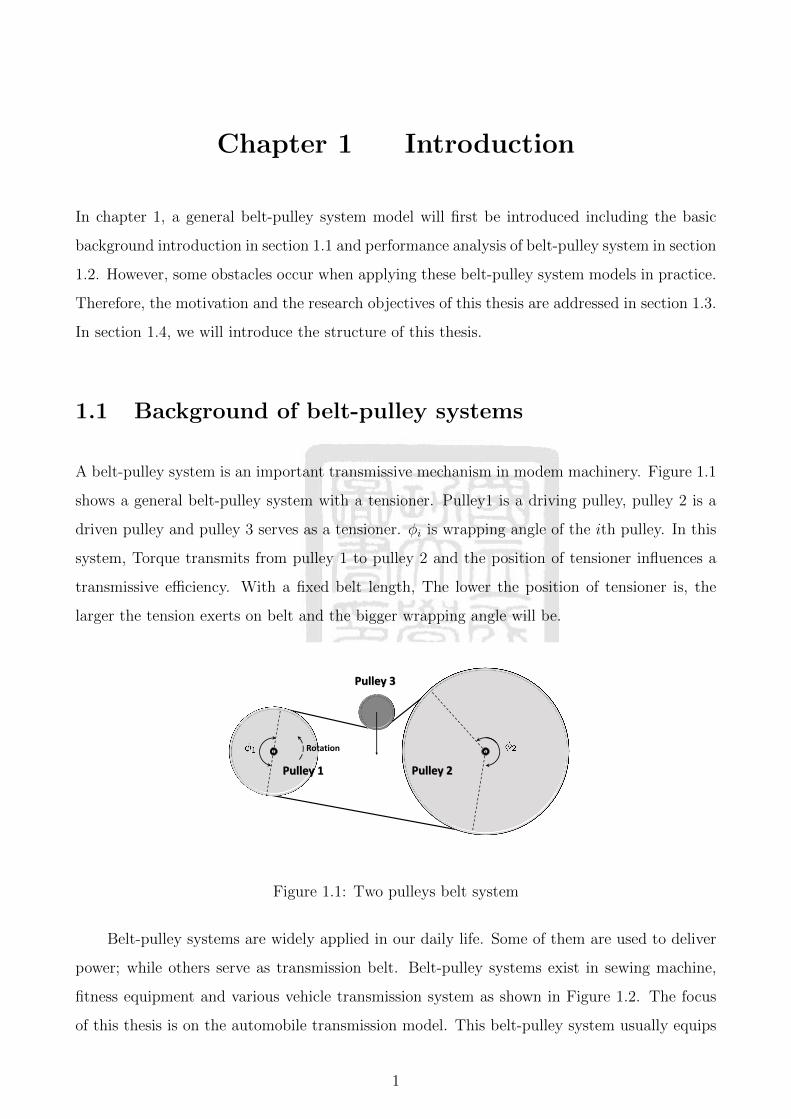
A belt-pulley system is an important transmissive mechanism in modem machinery. Figure 1.1

shows a general belt-pulley system with a tensioner. Pulley1 is a driving pulley, pulley 2 is a

driven pulley and pulley 3 serves as a tensioner. φi is wrapping angle of the ith pulley. In this

system, Torque transmits from pulley 1 to pulley 2 and the position of tensioner influences a

transmissive efficiency. With a fixed belt length, The lower the position of tensioner is, the

larger the tension exerts on belt and the bigger wrapping angle will be.

Pulley 1 Pulley 2

Pulley 3

Rotation

Figure 1.1: Two pulleys belt system

Belt-pulley systems are widely applied in our daily life. Some of them are used to deliver

power; while others serve as transmission belt. Belt-pulley systems exist in sewing machine,

fitness equipment and various vehicle transmission system as shown in Figure 1.2. The focus

of this thesis is on the automobile transmission model. This belt-pulley system usually equips

1

a tensioner to maintain sufficient tension to ensure transmitting torque from engine to gears is

acceptable. The position of the tensioner would effect transmissive efficiency as well as power

efficiency. When the tensioner provides overloading tension, the transmit efficiency might be

high but the power efficiency would be low, and vis versa. Therefore, a proper position balancing

transmit efficiency and power efficiency is an important issue.

Figure 1.2: Applications of belt-pulley system

1.2 Analysis of belt-pulley systems

After providing basic belt-pulley systems concept, let us look at the standard design guide-lines

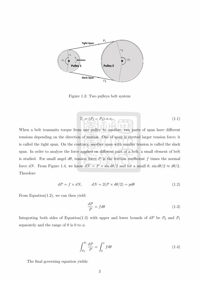
of belt-pulley systems [1,2]. These guide-lines usually starts with a general two pulleys system

as shown in Figure 1.3. A flat belt is treated as a string in traditional analysis of a belt-pulley

system. Pulley1 is a driving pulley and pulley 2 is a driven one. A part of flat belt between

two pulleys, span, is a straight line and tangents to pulleys. Contact points would be obtained

simply by analyzing a geometric outline of belt-pulley system. Ti is a torque on ith pulley , ri

is the radius of the ith pulley and P1 and P2 are tension forces. The relationship follows [1]:

2

Pulley 1 Pulley 2

Rotation

Tight Span

Slack Span

Figure 1.3: Two pulleys belt system

Ti = (P1 − P2)× ri (1.1)

When a belt transmits torque from one pulley to another, two parts of span have different

tensions depending on the direction of motion. One of span is exerted larger tension force; it

is called the tight span. On the contrary, another span with smaller tension is called the slack

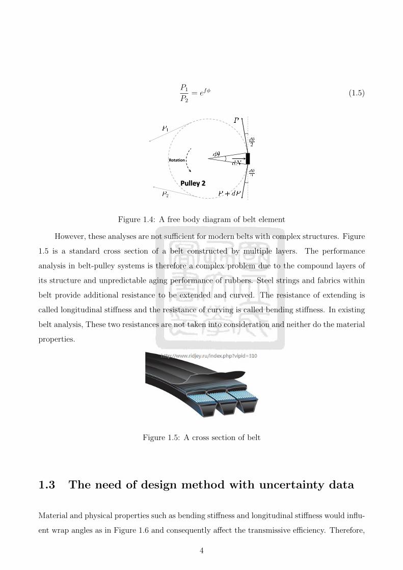
span. In order to analyze the force applied on different part of a belt, a small element of belt

is studied. For small angel dθ, tension force P is the friction coefficient f times the normal

force dN . From Figure 1.4, we know dN = P × sin dθ/2 and for a small θ, sin dθ/2 ≈ dθ/2.

Therefore

dP = f × dN, dN = 2(P × dθ/2) = pdθ (1.2)

From Equation(1.2), we can then yield:

dP

P= fdθ (1.3)

Integrating both sides of Equation(1.3) with upper and lower bounds of dP be P2 and P1

separately and the range of θ is 0 to φ.

∫ P1

P2

dP

P=

∫ φ

0

fdθ (1.4)

The final governing equation yields:

3

P1

P2

= efφ (1.5)

Rotation

Pulley 2

Figure 1.4: A free body diagram of belt element

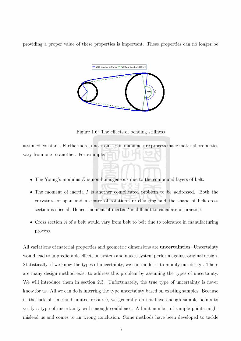
However, these analyses are not sufficient for modern belts with complex structures. Figure

1.5 is a standard cross section of a belt constructed by multiple layers. The performance

analysis in belt-pulley systems is therefore a complex problem due to the compound layers of

its structure and unpredictable aging performance of rubbers. Steel strings and fabrics within

belt provide additional resistance to be extended and curved. The resistance of extending is

called longitudinal stiffness and the resistance of curving is called bending stiffness. In existing

belt analysis, These two resistances are not taken into consideration and neither do the material

properties.

Figure 1.5: A cross section of belt

1.3 The need of design method with uncertainty data

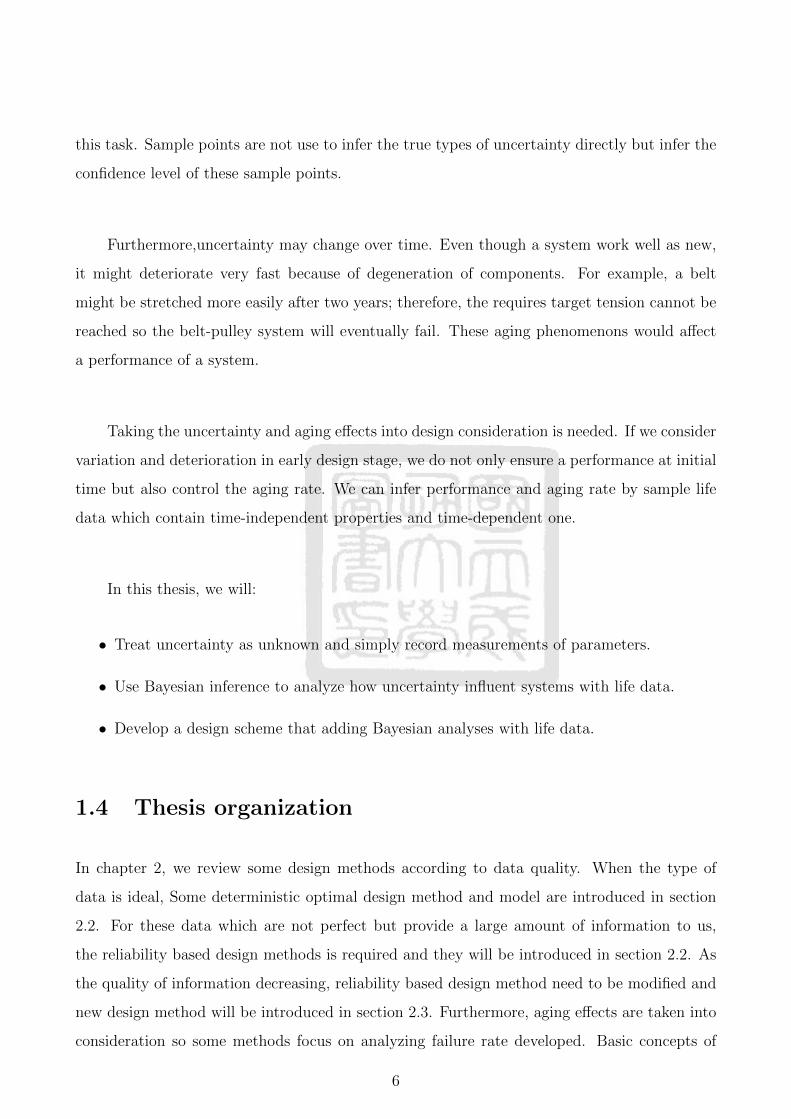
Material and physical properties such as bending stiffness and longitudinal stiffness would influ-

ent wrap angles as in Figure 1.6 and consequently affect the transmissive efficiency. Therefore,

4

providing a proper value of these properties is important. These properties can no longer be

With bending stiffness Without bending stiffness

Figure 1.6: The effects of bending stiffness

assumed constant. Furthermore, uncertainties in manufacture process make material properties

vary from one to another. For example:

• The Young’s modulus E is non-homogeneous due to the compound layers of belt.

• The moment of inertia I is another complicated problem to be addressed. Both the

curvature of span and a center of rotation are changing and the shape of belt cross

section is special. Hence, moment of inertia I is difficult to calculate in practice.

• Cross section A of a belt would vary from belt to belt due to tolerance in manufacturing

process.

All variations of material properties and geometric dimensions are uncertainties. Uncertainty

would lead to unpredictable effects on system and makes system perform against original design.

Statistically, if we know the types of uncertainty, we can model it to modify our design. There

are many design method exist to address this problem by assuming the types of uncertainty.

We will introduce them in section 2.3. Unfortunately, the true type of uncertainty is never

know for us. All we can do is inferring the type uncertainty based on existing samples. Because

of the lack of time and limited resource, we generally do not have enough sample points to

verify a type of uncertainty with enough confidence. A limit number of sample points might

mislead us and comes to an wrong conclusion. Some methods have been developed to tackle

5

this task. Sample points are not use to infer the true types of uncertainty directly but infer the

confidence level of these sample points.

Furthermore,uncertainty may change over time. Even though a system work well as new,

it might deteriorate very fast because of degeneration of components. For example, a belt

might be stretched more easily after two years; therefore, the requires target tension cannot be

reached so the belt-pulley system will eventually fail. These aging phenomenons would affect

a performance of a system.

Taking the uncertainty and aging effects into design consideration is needed. If we consider

variation and deterioration in early design stage, we do not only ensure a performance at initial

time but also control the aging rate. We can infer performance and aging rate by sample life

data which contain time-independent properties and time-dependent one.

In this thesis, we will:

• Treat uncertainty as unknown and simply record measurements of parameters.

• Use Bayesian inference to analyze how uncertainty influent systems with life data.

• Develop a design scheme that adding Bayesian analyses with life data.

1.4 Thesis organization

In chapter 2, we review some design methods according to data quality. When the type of

data is ideal, Some deterministic optimal design method and model are introduced in section

2.2. For these data which are not perfect but provide a large amount of information to us,

the reliability based design methods is required and they will be introduced in section 2.2. As

the quality of information decreasing, reliability based design method need to be modified and

new design method will be introduced in section 2.3. Furthermore, aging effects are taken into

consideration so some methods focus on analyzing failure rate developed. Basic concepts of

6

them are introduced in section 2.4. In chapter 3, we want to use Bayesian inference to analyze

the performance and aging process of a system. First, In section 3.1, A brief introduction of

Bayesian inference are shown including Bayes theorem in subsection 3.1.1 and two forms of

Bayesian inference; empirical and hierarchical Bayesian inference in subsection3.1.2 and 3.1.3.

Then, In section 3.2, illustrating what kind of prior in Bayesian inference is proper according to

what kind of data we have. Demonstration of Bayesian method applying reliability estimation

is shown in section 3.3. In chapter4, the analysis which is demonstrated in section 3.3 is adding

to design process. The flowchart of proposed design method present in section 4.1 and each step

in the flowchart will be introduced in the following section 4.2 to 4.4. In chapter 5, we apply

proposed design method to a mathematical example and a belt-pulley system design case. A

conclusion and future work are shown in chapter 6.

7

Chapter 2 Review of Belt-Pulley System

Analysis and Design Methods

2.1 Belt-pulley system performance analysis

There are two basic theories in the belt-pulley system analysis, namely shear theory [3–5] and

creep theory [5–7]. Creep theory is the original theory to analyze the performance of a belt-

pulley system and it is usually applied to soft belt such as those made of leather only. Soft belt

could perfectly fit the profile of pulleys and the span between any two pulleys can reasonably be

approximated as a straight line. However, belts we use nowadays are not leather belts anymore;

instead, they are made of layers of rubber, steel cores, and artificial textiles with the shape of

V. Features of V-belts differ much from leather belts. V-belt cannot wrap around the pulley

profiles perfectly and the span between two pulleys is a curve, not a straight line. Shear theory

has therefore been developed to deal with this new kind of belts. However, the calculation in

shear theory is too complicated to widely be applied.

In fact, these phenomena happen in V-belts mainly because of a material property of a

belt called bending stiffness. Some researchers try to take bending stiffness into consideration

when analyzing belt-pulley system with creep theory. Analysis of belt-pulley system in this

thesis is mainly based on creep theory considering bending stiffness by Parker et al [8,9].

We using a two-pulley belt system to illustrate the analysis process that can then be ex-

tended to general cases with multiple pulleys [8]. A belt is separated into three parts, namely

span, adhesion and sliding. Span represents part of a belt that dose not in contact with any

pulley. Adhesion zone is the part of a belt that moves in the same velocity with the pulley.

Finally, in the sliding zone, a velocity difference exists between sliding pat of belt and pulley.

In Figure 2.1, pulley 1 is the driver with driving torque M1. M2 is a loading exerting on pulley

2. αi is sliding angel, βi is adhesion angel on ith pulley. Behaviors of a belt are governed by

equations with different physical characteristics for different part of a belt. Material constants

8

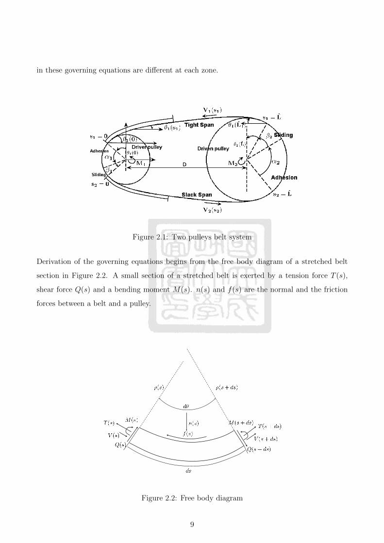
in these governing equations are different at each zone.

Figure 2.1: Two pulleys belt system

Derivation of the governing equations begins from the free body diagram of a stretched belt

section in Figure 2.2. A small section of a stretched belt is exerted by a tension force T (s),

shear force Q(s) and a bending moment M(s). n(s) and f(s) are the normal and the friction

forces between a belt and a pulley.

Figure 2.2: Free body diagram

9

This small section of a belt is treated as a moving Euler-Bernoulli beam and the Euler-Bernoulli

theory requires :

M = EIκ (2.1)

where EI is the bending stiffness, E is the Young’s modulus, I is the moment of inertia, and

κ is the curvature of the beam which also be defined as changing rate of inclination angle θ,

κ = dθ/ds. Since the beam is in a steady motion, forces acting on it should balance:

• The balance of angular momentum with respect to the center of mass of the small section

results in:

dM −Qds = 0, Q = dM/ds = EI(dκ/ds) (2.2)

• The balance of linear momentum in tangential direction results in:

dT − fds = GdV −Qdθ, G = m(s)V (s) = constant (2.3)

where m(s) is the mass density per unit length, For steady state, mass flow is conserved

so G =constant.

• The balance of linear momentum in normal direction results in:

(T −GV )dθ − dQ = nds (2.4)

From Equation(2.1) to Equation(2.4), we can yield the following two governing equations:

(T −GV )′ + EIκκ′ = f (2.5a)

(T −GV )κ− EIκ′′ = n (2.5b)

Equations(2.5) guide the behavior of the whole belt but a little different in each part. For

example, the friction force in Equation(2.5a) is different for sliding zone and adhesion zone be-

cause of the difference in static and kinetic frictional coefficient. Furthermore, for the span part,

the belt does not contact with any pulley so the contact forces f and n are zero. Equation(2.5)

is then transferred into:

(T −GV )′ + EIκκ′ = 0

(T −GV )κ− EIκ′′ = 0 (2.6)

10

Equation(2.5) is the main governing equations in belt-pulley system analysis. Other ge-

ometric boundaries are required when solving Equation(2.5). These boundaries are there to

ensure the belt exactly contacts with pulleys and they are orthogonal at the points of contacts.

The definition of boundary is shown in Figure 2.1.

Let T −GV = W . Seven differential equations and seven boundaries are shown as following:

• Physical differential equations:

– dW/ds = EIκκ′ − f , derived from Equation(2.5a).

– dκ/ds = (f −W )/κ× EI, derived from Equation(2.5a).

– d2κ/ds2 = (W − n)/EI, derived from Equation(2.5b).

• Geometric differential equations:

– dθ/ds = κ, it is the definition of curvature.

– dx/ds = cos θ, x is a position on x-axis.

– dy/ds = sin θ, y is a position on y-axis.

– dL/ds = 0, L is the length of span in steady motion and it is a constant.

• Boundary conditions:

– W (0) = T (0)−GV (0), the initial value of span closed to pulleyi

– κ(0) = 1/Ri, at points of contacts, the curvature of belt is equal to which of pulleys.

– κ(L) = 1/Ri+ 1

– x(0) = Ri sin(θ(0)), ensuring the belt is orthogonal to pulleys.

– x(L)−D = Ri+1 sin(θ(L))

– x(0)2 + y(0)2 = Ri, ensuring the belt contact with pulleys.

– x(L)− L2 + y(L)2 = Ri+1

By solving this boundary value problem, we can yield W , θ, κ, κ′,x and y.Detail of solving

process will be introduced in section 5.2.

11

2.2 Design methods with ideal data

After describing the analysis of belt-pulley system, let us switch topic to general design methods

of engineering product.Theoretically, we can improve the quality and performance of an engi-

neering product by optimization. We set an objective function(f) and several constraints (gi)

and then minimize the objective function subject to these constraints within the design upper

(dU) and lower bounds (dL). When parameters (p) are constants, we can yield an optimal

design(d∗) by solving the optimization problems posed as :

mindf(d,p)

s.t. gi(d,p) ≤ 0, i = 1 ∼ n (2.7)

dL ≤ d ≤ dU

2.3 Design methods with abundant data

In reality, uncertainty exists in manufacturing process, in material properties, and in the vari-

ation of environment, some parameters P may not be constants anymore. Parameters would

vary in a small range.These unpredictable effects are called uncertainty. When design process

involves uncertainty, the original optimal process is transferred into a probabilistic optimal

design format [10–12] as in Equation(2.8) which are referred to as reliability-based design op-

timization (RBDO). Equation(2.8) is a generalized single-objective probabilistic formulation

with random design variables D, random parameters P, deterministic design variables d and

deterministic parameters p. The objective f is a function of the deterministic quantities and

the mean values of random quantities in the formulation. The feasible space of d subject to

all constraints in K is F . The reliability of a design is defined as the probability of satisfying

constraints, denoted as 1− Pf

minµD,d

f(µD,µP,d,p)

Pr[gj(D,P,d,p) > 0] ≤ Pf,j ∀j ∈ K (2.8)

Solving the probabilistic constraint require an additional analysis to the conventional opti-

12

mal design process. Therefore, the solution complexity and the computational cost are increas-

ing. Standard approaches in solving this probabilistic constraints include: the first/second order

reliability method (FORM/SORM) [13–15], adaptive importance sampling [16], advance mean

value [17], and its hybrid variant [18], sequential optimization and reliability assessment [19],

and single-loop method [20]. Furthermore, many methods have been proposed to enhance nu-

merical efficiency and stability in solving RBDO problems [21–23].

2.4 Design methods with inadequate data

Applying the probabilistic methods mentioned in section2.3 requires the distribution of the

uncertainty or the aging process be known as a priori. Unfortunately, it is impractical to

know the exact distributions of uncertainty or the aging process; the conventional methods, are

therefore limited in its industrial practice.

Instead of have the distribution information, we usually have only limited measurement

samples of these uncertainty. These sample points are measurements drawn from specific dis-

tribution and the type of distribution is unknown to us. Some researchers use sample points to

infer the unknown distribution of uncertainty. The inference generates large errors when the

sample points are inadequate or type of distribution we assumed is improper [24–26]. Other

researchers analyze reliability without inferring the distributions of uncertainty; they use the

concept of confidence in design, such as possibility-based design optimization (PBDO) [27,28]

based on possibility theory [29–34], evidence-based design optimization (EBDO) [35] based on

evidence theory [36–38], and Bayesian RBDO [39–41] based on Bayes theory [42–45].

In Bayesian RBDO, the analysis of confidence levels based on data is added into the

reliability-based optimization process. The generalized Bayesian optimization model can be

13

expressed as:

minµDu ,d

f(µDu ,d,Ps,µPu ,p)

s.t gi = gi(d,p) ≤ 0

gR = Pr[gi(Du,d,Pu,p) ≤ 0] ≥ Rt

gB = Pr[Pr[gi(Du,d,Pu,Ps,p) ≤ 0] ≥ Rt

]≥ CRt

(2.9)

where

d : deterministic design variables

Du : uncertain design variables with known distributions

p : deterministic parameters

Pu : uncertain parameters with known distributions

Ps : uncertain parameters with samples

g : deterministic constraint

gR : reliability constraints with reliability target

gB : Bayesian reliability constraints with a reliability target and a confidence range target

The main idea of Bayesian inference is that a posterior distribution is proportional to the

product of likelihood and prior distribution [39]. The prior is an initial guess of distribution

about on uncertainty, the posterior is an inferred distribution according to some observations,

and the likelihood can be treated as a weighting between posterior and prior. The type of prior

would effects final result of posterior so some researchers try to figure out how to choose the

proper prior when applying Bayesian inference [46].

Computational operation in Bayesian inference sometimes could be very expensive. Con-

jugate prior could help us get arid of expensive computation. We could obtain a posterior

distribution by changing the parameters of prior distribution instead of by multiple integra-

tion. Different types of conjugate prior we choose could address different kind of problems. For

instance, the Binomial-Beta inference choosing beta distribution as a prior distribution and

14

Binomial distribution as likelihood is mainly use to address problem with pass/fail data at a

specific time instant [39]. Moreover, the Poisson-Gamma inference setting a Gamma prior and

Poisson likelihood is frequently applied to calculate the probability of failure given a failure rate

and an expected failure number. Bayesian inference could deal with both time-independent and

time-dependent problem by choosing different conjugate priors.

2.5 Design methods with life data

A good product is not only reliable but also durable; that means low probability of failure at

the initial time and low failure rate throughout the life span. Figure 2.3 shows a typical failure

probability curve with respect to time. The solid curve is the current design and the dash

line is the design with improved reliability, which has low probability of failure and small the

increment of failure rate.

Steady failure rate

Aging

Figure 2.3: Bathtub curve in product reliability

After including time-factor in design, the RBDO and Bayesian RBDO are transferred into

time-dependent RBDO and time-dependent Bayesian RBDO. The general mathematical for-

mulation can be expressed as:

15

minµDu ,d

f(µDu ,d,Ps,µPu ,p)

s.t gi = gi(d,p) ≤ 0

gR = Pr[gi(Du,d,Pu,p) ≤ 0] ≥ Rt

gB = Pr[Pr[gi(Du,d,Pu,Ps,p) ≤ 0] ≥ Rt

]≥ CRt

gi(t) = git(d,p,p(t)) ≤ 0

gR(t) = Ra(Du,d,Pu,p,Du(t),Pu(t),p(t)) ≥ Pt(t)

gB(t) = Pr [Ra(Du,d,Pu,p,Du(t),Pu(t),p(t)) ≥ Pt(t)] ≥ CLt(t)

(2.10)

where

d : deterministic design variables.

Du : uncertain design variables with known distributions.

Du(t) : time-dependent uncertain design variables with known distributions.

p : deterministic parameters.

p(t) : time-dependent deterministic parameters.

Pu : uncertain parameters with known distributions.

Pu(t) : time-dependent uncertain parameters with known distributions.

Ps : uncertain parameters with samples.

Ps(t) : time-dependent uncertain parameters with samples.

g : deterministic constraint.

gR : reliability constraints with a reliability target Rt.

gB : Bayesian reliability constraints with a reliability target Rt and a confidence range

target CRt.

g(t) : time-dependent deterministic constraint.

gR(t) : time-dependent reliability constraints with a reliability target Pt.

16

gB(t) : time-dependent Bayesian reliability constraints with a reliability target Pt and a

confidence range target CLt.

Ra : the reliability of aging process which is inferred based p, p(t), Pu, Pu(t), Ps and

Ps(t).

Rt and Pt : the reliability target for time-dependent and time-independent cases.

CRt and CLt : the confidence range target for time-dependent and time-independent

cases.

Three basic approaches have been proposed to deal with time-dependent reliability-based

optimization, namely the extreme performance approach, the first-passage approach, and the

composite limit state approach. In extreme performance approach, response surfaces of con-

straints and the objective function are built to reach a maximal improvement of a performance

criteria, i.e., the accuracy. Although the performance of a response surface is updated by

adding new samples as shown in [47], these approaches isolate time factor instead of consid-

ering time-varying characteristics. In other words, the aging model is known. Another widely

applied method is the first-passage approach. The general concept of the first-passage approach

uses the up-crossing rate to evaluate the probability of failure over a period of time when ini-

tial failure occurred [47,48]. However, the up-crossing rate is hard to calculate so there are

some methods developed to reduce computational efforts [48]. The third method to address

a time-dependent RBDO is the composite limit state approach [49] that divides a time inter-

val into finite time periods and transfers a time-dependent problem into a time-independent

equivalence [47]. Note that the extreme performance approach, the first-passage approach, and

the composite limit state approach can be applied to both inferences with abundant data and

inadequate data.

Other relevant approach about time-dependent reliability analysis focus inferring the fail-

ure rate. For example, Colombo et al. presented nonparametric estimation of time-dependent

failure rates with life data [50]. Semi-parametric bathtub-curve failure rate was proposed by

Ho [51]. However, nonparametric estimation and Semi-parametric of failure rate require a

abundant of data, but sometimes we are not able to get so much data to construct model

accurately.

17

Chapter 3 Bayesian Inference in Reliability

Analysis with Mixed Data Types

The main goal of this research is to systematically incorporate measured data within the design

process. The central idea behind this process is the Bayesian updating scheme. In this chapter,

Bayes theorem would be introduced in section 3.1 followed by two types of conjugate prior

to address time-independent and time-dependent problem in section 3.2. The procedure of

reliability estimation is presented step by step in section 3.3. Finally, an constraints reliability

estimation example is demonstrated in section 3.4.

3.1 Introduction of Bayesian inference

Uncertainties are omnipresent in design process and designers usually assume they know the

underlying distributions of uncertainties. However, the underlying distribution is never know

to us. When an assuming distribution differs from the true underlying distribution, inference

would lead to wrong results. Even if the type of distribution assumed is correct, inferring under-

lying distribution with limit number of samples might be misled by bias samples. Therefore, a

confidence range of these data is calculated as an expression of the degree of trust on measured

data. Bayesian inference is the approach based on Bayes theorem to estimate the confidence

range of data. In what follows, we will talk about Bayes theorem first.

Bayes theorem

Bayes theorem is the rule based on conditional probability as in Equation(3.1):

Pr(A|B) =Pr(A ∩B)

Pr(B)(3.1)

where Pr(A|B) is the probability of an event A happening given event B, Pr(B) is the probability

of an event B, and Pr(A ∩ B) is the joint probability of both events A and B. Furthermore,

Pr(A∩B) = Pr(B|A) Pr(A) is known as multiplication rule can transfer Equation(3.1) into

Equation(3.2):

Pr(A|B) =Pr(B|A) Pr(A)

Pr(B)(3.2)

18

Define Pr(A|B) as the posterior probability, Pr(B|A) as the likelihood, and Pr(A) as the prior

probability. According to Equation(3.2), Pr(A|B) ∝ Pr(B|A) Pr(A). This is the basic concept

of Bayes inference, which states: the posterior probability is in proportion to the product of

the prior and the likelihood.

If events A and B follow binomial process, the formula in Equation(3.2) could be ex-

pressed in another form. We denote Pr(Ac) as the complement probability of the event A. The

probability of the event B happening can be denoted as Equation(3.3)

Pr(B) = Pr(B ∩ A) + Pr(B ∩ Ac) (3.3)

Applying multiplication rule to each joint probability, we can rewrite Equation(3.2) as:

Pr(A|B) =Pr(B|A) Pr(A)

Pr(B)=

Pr(B|A) Pr(A)

Pr(B|A)× Pr(A) + Pr(B|Ac)× Pr(Ac)(3.4)

In more general cases with multiple events, we then have:

Pr(B) =k∑j=1

Pr(B|Aj) Pr(Aj) (3.5)

Conditional probability of multiple events results in Equation(3.6).

Pr(Aj|B) =Pr(B|Aj) Pr(Aj)∑kj=1 Pr(B|Aj) Pr(Aj)

(3.6)

Equation(3.6) is the general form of Bayes theorem. The form also express the basic idea of

Bayes inference:

Posterior Probability ∝ Prior Probability × Likelihood

Note that when applying the Bayes inference, the prior probability, Pr(Aj), can be treat as

the bound of previous known information, the posterior, Pr(Aj|B), can be treated as the

inferred result based on known information, and the likelihood, Pr(Aj|B), presents the similarity

between the prior and the posterior.

3.2 Prior selection based on data types

The types of prior distribution and of likelihood result in different type of posterior distributions.

In some special cases, the types of prior and posterior distributions are the same; these priors are

19

called conjugate priors. The biggest advantage of conjugate priors is the parameter calculation

with known distributions. Beta-binomial and Poisson-gamma are the common used conjugate

priors. We will introduce the use of beta-binomial to infer time-invariant uncertainty data in

Section 3.2.1 and the use of Poisson-Gamma to infer time-variant life data in Section 3.2.2

3.2.2, respectively.

3.2.1 Time invariant measurement data

When the prior distribution follow a beta distribution and the likelihood follow the binomial

process, the posterior distribution will also be a beta distribution, a standard process called

beta-binomial inference. Beta-binomial inference usually applies in binary tests such as pass/fail

test at a time instant.

Beta Distribution

Beta distribution is a continuous distribution defined on the interval [0,1], with two positive

parameters α and β

as in Equation (3.7) where Γ(·) is the Gamma function.

f(p|r) =Γ(α + β +N)

Γ(α + r)Γ(N − r + β)p(r+α−1)(1− p)(N−r+β−1) (3.7)

Taking the average death rate of a disease for instance, p represents the average death rate and

f(p|r) is the probability of the expected death rate occurring given the observed death number.

Note that beta distribution with parameters (1,1) is an uniform distribution, that means all

the probability of expected probability is the same.

Binomial Distribution

Binomial distribution is frequently used as to model the probability of a specific number of

marked sample occurring given a probability of expected average in a binary experiment. Let

r be the number of success, N be the total sample number, and p be the average probability

of success in Equation (3.8). Furthermore, f(r|p) means a probability of success number is

exactly r given an average probability p.

f(r|p) =

N

r

pr(1− p)N−r (3.8)

20

for r = 0, 1, · · · , N where N

r

=N !

r!× (N − r)!

Coin flip is a simple example to illustrate the general idea of binomial distribution. A coin is

tossed 10 times and the average probability of getting heads is 0.5 in a fair toss. The expected

number of head is 5 but there still have a chance to get 3 heads only. According to Equation

(3.8), the probability of getting 3 heads out of 10 tosses is f(3|0.5) = 0.1172.

Beta-Binomial Inference

When the prior distribution follows beta distribution and likelihood being binomial distribution,

the general Bayes theorem in Equation (3.6) is transferred into Equation (3.9).

f(p|r) =f(r|p)× f(p)∫ 1

0f(r|p)f(p)dp

(3.9)

f(r|p) is a binomial distribution and f(p) is a beta distribution. N is the total number of

sample set r is the number of success we observed and p is the probability of success outcome

occurred.∫ 1

0f(r|p)f(p)dp is a normalizing factor that ensure the range of posterior within [0,1].

f(p|r) =Γ(α + β +N)

Γ(α + r)Γ(N − r + β)p(r+α−1)(1− p)(N−r+β−1) (3.10)

Equation (3.10) is the standard form of beta distribution with parameter α′ = α + r, β′ =

β +N − r. :

f(p|r) = φbeta(α′, β′) (3.11)

From Equation (3.11), the biggest advantage of beta-binomial inference is that the posterior

PDF can be obtained by counting the number of successes and total sample number without

integration. When we have no idea about the probability of success, f(p), we usually set the

original parameters(α, β)=(1,1), an uninformative uniform prior. By adding sample data, the

reliability estimation will be continuously updated by counting number of success r and total

sample number N .

3.2.2 Time variant life data

Assuming that the failure rate of a system is a constant over time, therefore, the time of the nth

failure occurring can accurately be estimated. However, in reality, the true failure rate is not

21

known due to the lack of data. The failure rate is therefore some distribution and the time of the

nth failure is also follows some types of distribution. In this thesis, we infer the probability of

failure rate based on observations at different time instant using the Poisson-gamma inference.

The Poisson-gamma inference is frequently applied to infer failure rate within an interval

of time according to the observed failure number. We will introduce Poisson distribution and

gamma distribution separately and then derive the general form of posterior distribution based

on Bayesian inference. The posterior distribution is the failure rate given the observations that

can be used to estimate the time of the nth failure.

Poisson Distribution

Poisson distribution is a discrete distribution frequently used to predict the probability of

expected number of failure event occurring given a failure rate in a time or space interval.

When each probability of event occurring is independent. The PDF is:

f(k;λ) =λk

k!× e(−λ) for k = 1, 2, 3, · (3.12)

where λ > 0 is the average failure rate within a time interval and k is the expected number of

failure events in the same interval.

Gamma Distribution

Gamma distribution belongs to exponential distribution family with two parameters, a shape

parameter a and a rate parameter b. It is commonly applied to model rainfall or waiting time.

In this thesis, gamma distribution is use as prior of failure rate λ. The Gamma PDF is:

f(λ; a, b) = ba1

Γ(a)λa−1e−bλ (3.13)

where Γ(·) is the Gamma function. Note that when the shape parameter a = 1, gamma distri-

bution will become an exponential distribution with a rate parameter b.

Poisson-Gamma Inference

Poisson-Gamma inference is mainly used to infer the failure rate based on life data in this

thesis. With the prior distribution f(λ) be a gamma distribution and the likelihood f(k|λ) be

a Poisson distribution, the posterior is shown in Equation(3.14).

f(λ|k) =f(k|λ)× f(λ)∫∞

0f(k|λ)× f(λ)dλ

(3.14)

22

Substitute PDF of Poisson and Gamma distributions into and Equation(3.14) results as in

Equation(3.15):

f(λ|k) =

e−λλk

k!ba

Γ(a)λa−1e−λb∫ 1

0e−λλk

k!ba

Γ(a)λa−1e−λbdλ

(3.15)

where ∫ ∞0

e−λλk

k!

ba

Γ(a)λa−1e−λbdλ =

1

k!

ba

Γ(a)

Γ(k + a)

(b+ 1)k+a(3.16)

Substitute Equation(3.16) into (3.15), we see that the posterior distribution become a Gamma

distribution with new parameters of a′ = a + k and b′ = b + 1. When the interval of time is

divided into ng sections, the parameters is a′ = a+∑ng

i=1 k1 and b′ = b+ ng:

f(λ|k) = φgamma(a′, b′) (3.17)

f(λ|k) is the density function of failure rate given observed failure number. By to Poisson

counting process, if the number of failure is assumed to follow a Poisson distribution, the

waiting time T [c] until the cth failure occurring is a Erlang distribution. The CDF of Erlang

distribution, Pr(T [c] ≤ t), is the probability of the time of the cth failure earlier than the time

t, as shown in Equation(3.18):

Pr(T [c] ≤ t) = ΦErlang(t; c, λ) = 1−c−1∑n=0

1

n!(λt)ntn−1e−λt (3.18)

A more reliability product has less number of failures within the same time interval compared

with its competitors. Therefore, the reliability of aging process, Ra, is the probability of the

failure number is less than c before at time t. Pr(T [c] ≥ t).

Ra = Pr(T [c] ≥ t) = 1− ΦErlang(t; c, λ) =c−1∑n=0

1

n!(λt)ntn−1e−λt (3.19)

where t is the time period we are interested in and c is the critical failure number. When the

failure rate λ is a constant, Pr(T [c] > t) is a fixed value. However, when the failure rate is a

gamma distribution inferred from Poisson-Gamma inference in this thesis, Pr(T [c] > t) is also

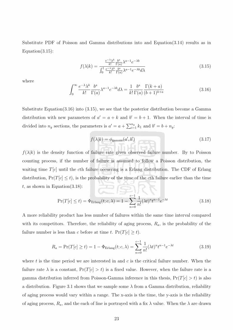
a distribution. Figure 3.1 shows that we sample some λ from a Gamma distribution, reliability

of aging process would vary within a range. The x-axis is the time, the y-axis is the reliability

of aging process, Ra, and the each of line is portrayed with a fix λ value. When the λ are drawn

23

Time

t

Density

CDF of T[n]

𝑹𝒂

Figure 3.1: An illustration of the effect of parameter with distribution

from a gamma distribution and the sample size of λ is large enough, the PDF of reliability of

aging process could be yielded.

In this thesis, beta-binomial inference is applied to estimate the reliability of an engineering

design at the initial state. The Poisson -Gamma inference is used to estimate the failure rate

of this function given the observed failure number. The failure rate is further used to estimate

the failure probability within a period of time.

3.3 Reliability estimation using Bayesian inference with

life data

Constraints in the engineering design contain some parameters with uncertainty. In reality,

we can only get few measurements of the parameters. Therefore, these measurements need

to be accounted for to estimate the reliability of the constraints by inferences which have

been introduced in section 3.2. In this thesis, the basic inferring process will be introduced in

subsection 3.3.1. Confidence range and confidence bound will be introduced in the inferring

process in subsection 3.3.2. A mathematical example will be used to demonstrate the inferring

process in section 3.4.

24

3.3.1 Reliability estimation of constraints

Let the number of time invariant samples P1 be N0, of the time variant samples P2(t) be N2(t) at

time t, and of the time variant samples P3(t) is N3(t) at time t.The time-independent samples,

P1, could combine with each sample at any time instant as they will not changed over time.

However, time-dependent samples can only combine with samples which are measured at the

same time. Therefore, we can denote the sample sets we obtain at time t be (P1, P2(t), P3(t))

at time t. For example, the number of the time invariant samples is N0 = 3, the time interval

now is divided into two segment, t1 and t2, the number of segments of time interval,Ng, is 2.

The numbers of the time variant samples P2 are N2(t1) = 3 and N2(t2) = 4 , and the numbers

of the time variant samples P3 are N3(t1) = 2 and N3(t2) = 3. Therefore, the number of

sample sets Nc(t) at t1 is Nc(t1) = 3 × 3 × 2 = 18, and the number of sample sets at t2 is

Nc(t2) = 3× 4× 3 = 36.

Some samples would make the value of a constraint being less than zero, and some samples

would make the value of a constraint being greater than zero. We define a constraint being less

than zero a success event. Therefore, we can have the number of success based on the total

number of samples at t.

Beta-binomial inference requires the number of success r and the number of sample set

Nc(t1) at initial time t1. while Poisson-gamma inference requires the total number of failure

at all time instant∑Ng

i=1 ki and the number of the time interval Ng. With these distribution

parameters beta-binomial inference becomes:

f(R|r) = φbeta(α + r,Nc(t1)− r + β) (3.20)

and the Poisson-gamma inference becomes:

f(λ|k) = φgamma(a+

Ng∑i=1

ki, b+Ng) (3.21)

Equation(3.20), we can infer the distribution of reliability R when observer r success and from

25

Equation(3.21), the distribution of the failure rate λ given current number of failure k. The

If the distribution of some design parameters are known, the beta-binomial inference and

Poisson-gamma inference is modified slightly. In the previous case mentioned in the beginning

of this subsection, tests of each sample set are defined as pass/fail with reliability being 1 or 0.

Therefore, we can simply count the number of successful samples and use the value as number

of success r.

Consider a performance function g with design parameters with both distribution, Pu and

with samples, Ps, the reliability of the constant with the ith sample set for Ps is:

Ri = Pr[g(Xu,Pu)|(Xs,Ps)i ≤ 0] (3.22)

Figure 3.2 illustrate the case with three samples combined with distribution design parameter.

The area on the left hand side of g = 0 is the reliability value. As shown, that reliability value

depend on the design parameter samples.The expected total number of success r is:

E[r] =N∑i=1

Ri (3.23)

Figure 3.2: An image of reliability given distribution with ith sample data

The expression of beta-binomial inference with distribution and sample design parameters is:

R ∼ φbeta(E[r] + α,N1 − E[r] + β) (3.24)

Similar idea can be applied to estimate the number of failure using Poisson-gamma inference.

In Figure 3.2, the area on the right hand side of g = 0 is the failure probability and sum up

the failure probability given the design parameter samples, the expected failure number, E[k],

26

is yielded. The k in Equation (3.21) are replaced by E[k].

λ ∼ φgamma(

ng∑i=1

E[k]i + a, b+ ng) (3.25)

By counting the exact or the expected failure number, the distribution of failure rate is

yield. The failure rate can be used to estimate the reliability of an aging process, Ra.

Ra = Pr(T [c] ≥ t) = 1− ΦErlang(t; c, λ) =c−1∑n=0

1

n!(λt)ntn−1e−λt (3.26)

where t the is usually warranty we set, the c is the maximum acceptable number of failure.

Furthermore, warranty and the max failure number are fixed value but the parameter λ is

a distribution that we yield from Poisson-gamma inference. Since λ is a distribution, the

reliability of aging process is also a distribution.

Follow the process mentioned in subsection 3.3.1, we can analyze a the reliability of a

constraint with life data in both initial state and aging process. This analysis can be used

in a design process so that we can control the quality of a design at initial state and ensure

the failure number of failure within a time interval is less than specific number; it is a similar

concept to warranty.

3.3.2 Definition of confidence range and confidence bound

Confidence range is the degree of confidence of the reliability from the inference with sample

data. In beta-binomial inference, the distribution of reliability R is yielded from Equation

(3.20). Setting a critical value Rt and the probability of R greater than Rt, Pr(R ≥ Rt), is

called the confidence range of reliability, CRR, shown in Equation(3.27):

CRR = Pr(R ≥ Rt) = 1− Φbeta(Rt, α, β) (3.27)

When assuming all the samples are successful events, we can get the maximum confidence range

of reliability, is also named confidence bound of reliability, CBR.

CBR = max[Pr(R ≥ Rt)] = 1− Φbeta(Rt, N1 + 1, 1) (3.28)

27

According to Equation (3.28), CBR is only associated with reliability targetRt and total number

of samples N1. If the confidence bound of reliability CBR is less than confidence range target,

CRt, we assign, we have to increase the number of samples.

The similar concept can be applied to Poisson-gamma inference. The reliability of and

aging process is denoted as Pr(T [c] ≥ t) = Rf , the reliability target of an aging process

is symboled as Pt and the probability of the reliability of aging process being larger than a

probability target is defined as confidence range of an aging process, CRf . The expression of

CRf is shown:

CRf = Pr[Pr(T [c] ≥ t) ≥ Pt] = Pr[Ra ≥ Pt] (3.29)

Assuming all current samples are safe, the failure rate inferred will bw the lowest failure rate

one can expect. This lowest failure rate can infer the probability of the cth failure occurring,

T [n], being later than the time we set of an aging process. The maximum confidence level is

called the confidence bound of failure.

CBf = max[Pr[Ra ≥ Pt]] (3.30)

CBf is the highest value of confidence level under current sample number. When confidence

bound of failure CBf is less than confidence level target CLt, this target are impossible to reach

with handing samples. Therefore, adding new samples is necessary.

3.4 Reliability estimation example

Taking a constraint G(P1, P2) = 1 − 80/(P 21 + 8 × P2 − 6) for demonstrating example where

P1 is time invariant parameter, P1 ∼ N(−8.2, 0.082), and P2 would deteriorate over time,

P2 ∼ N(2.2 × e−t, 0.022). Furthermore, the target probability are 0.7 for both reliability and

failure, Rt = 0.7 and Pf = 0.7. Then, calculating the confidence range of reliability that relia-

bility distribution greater than Rt, CRR = Pr[R > Rt]; also calculating the confidence range of

reliability of aging process, CRf = Pr[Ra > Pt]. There are two cases to verify how increments

of sample size of time invariant and variant parameters will affect the confidence ranges of

reliability in both initial state and aging process.

28

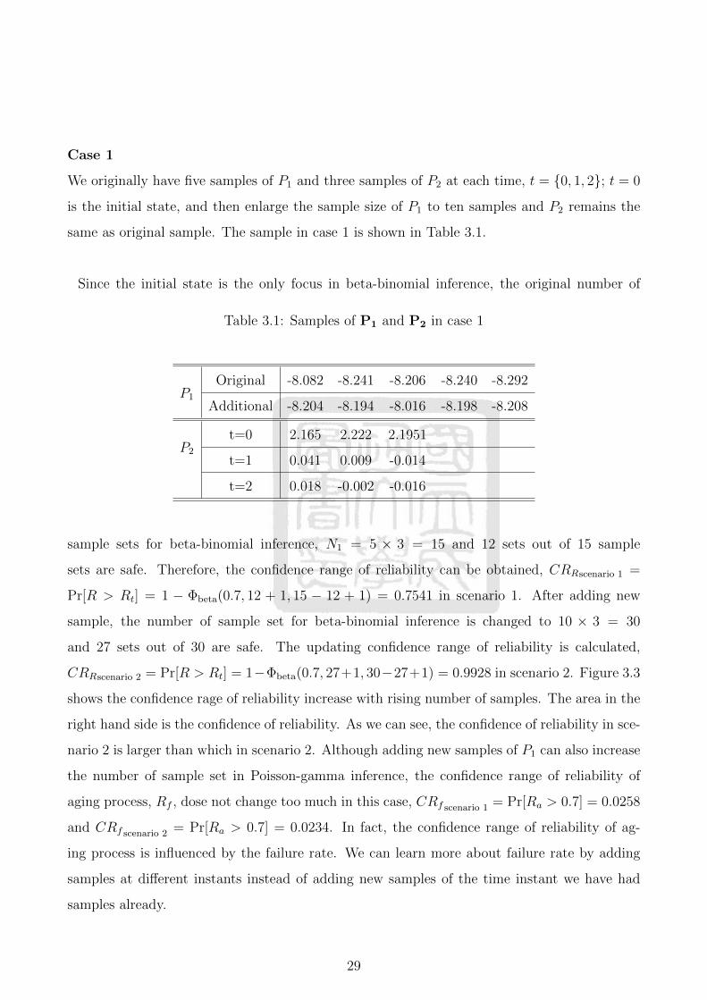
Case 1

We originally have five samples of P1 and three samples of P2 at each time, t = {0, 1, 2}; t = 0

is the initial state, and then enlarge the sample size of P1 to ten samples and P2 remains the

same as original sample. The sample in case 1 is shown in Table 3.1.

Since the initial state is the only focus in beta-binomial inference, the original number of

Table 3.1: Samples of P1 and P2 in case 1

P1

Original -8.082 -8.241 -8.206 -8.240 -8.292

Additional -8.204 -8.194 -8.016 -8.198 -8.208

P2

t=0 2.165 2.222 2.1951

t=1 0.041 0.009 -0.014

t=2 0.018 -0.002 -0.016

sample sets for beta-binomial inference, N1 = 5 × 3 = 15 and 12 sets out of 15 sample

sets are safe. Therefore, the confidence range of reliability can be obtained, CRRscenario 1 =

Pr[R > Rt] = 1 − Φbeta(0.7, 12 + 1, 15 − 12 + 1) = 0.7541 in scenario 1. After adding new

sample, the number of sample set for beta-binomial inference is changed to 10 × 3 = 30

and 27 sets out of 30 are safe. The updating confidence range of reliability is calculated,

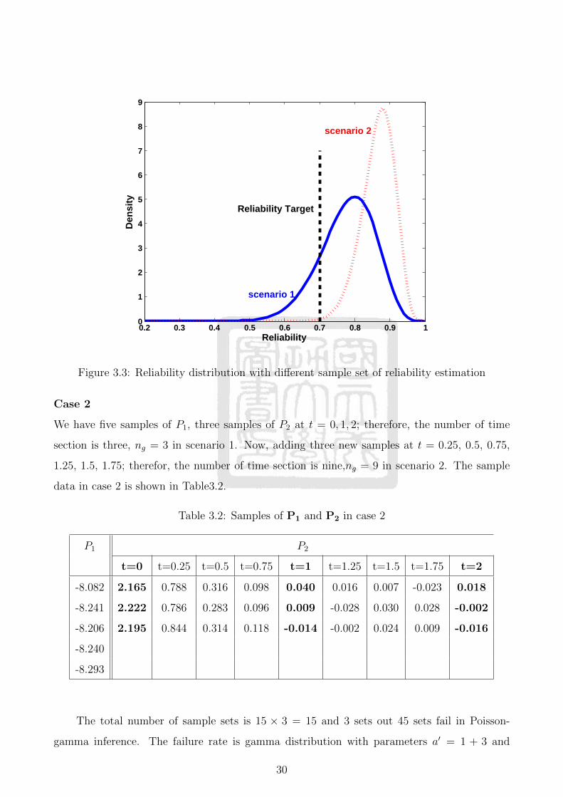
CRRscenario 2 = Pr[R > Rt] = 1−Φbeta(0.7, 27+1, 30−27+1) = 0.9928 in scenario 2. Figure 3.3

shows the confidence rage of reliability increase with rising number of samples. The area in the

right hand side is the confidence of reliability. As we can see, the confidence of reliability in sce-

nario 2 is larger than which in scenario 2. Although adding new samples of P1 can also increase

the number of sample set in Poisson-gamma inference, the confidence range of reliability of

aging process, Rf , dose not change too much in this case, CRf scenario 1 = Pr[Ra > 0.7] = 0.0258

and CRf scenario 2 = Pr[Ra > 0.7] = 0.0234. In fact, the confidence range of reliability of ag-

ing process is influenced by the failure rate. We can learn more about failure rate by adding

samples at different instants instead of adding new samples of the time instant we have had

samples already.

29

0.2 0.3 0.4 0.5 0.6 0.7 0.8 0.9 10

1

2

3

4

5

6

7

8

9

Reliability

Den

sity

Reliability Target

scenario 2

scenario 1

Figure 3.3: Reliability distribution with different sample set of reliability estimation

Case 2

We have five samples of P1, three samples of P2 at t = 0, 1, 2; therefore, the number of time

section is three, ng = 3 in scenario 1. Now, adding three new samples at t = 0.25, 0.5, 0.75,

1.25, 1.5, 1.75; therefor, the number of time section is nine,ng = 9 in scenario 2. The sample

data in case 2 is shown in Table3.2.

Table 3.2: Samples of P1 and P2 in case 2

P1 P2

t=0 t=0.25 t=0.5 t=0.75 t=1 t=1.25 t=1.5 t=1.75 t=2

-8.082 2.165 0.788 0.316 0.098 0.040 0.016 0.007 -0.023 0.018

-8.241 2.222 0.786 0.283 0.096 0.009 -0.028 0.030 0.028 -0.002

-8.206 2.195 0.844 0.314 0.118 -0.014 -0.002 0.024 0.009 -0.016

-8.240

-8.293

The total number of sample sets is 15 × 3 = 15 and 3 sets out 45 sets fail in Poisson-

gamma inference. The failure rate is gamma distribution with parameters a′ = 1 + 3 and

30

b′ = 1 + 3; therefore, the mean of failure rate is a′/b′ = 1. Using this failure rate which is

a distribution, we can yield confidence range of reliability of aging process by MCMC algo-

rithm, CRfscenario1 = Pr[Ra > 0.7] = 0.0258. After that, adding additional tree samples at

t = 0.25, 0.5, 0.75, 1.25, 1.5, 1.75, time interval is divided into 9 section, ng = 9. The total num-

ber of sample sets is 15× 9 = 135 and 3 sets out of 135 fail. we can infer the new distribution

of the failure rate; the new failure rate is a gamma distribution with parameters a′ = 1 + 3 and

b′ = 1 + 135, and the mean of the new failure rate is E[λ] = a′/b′ = 4/136. Furthermore, The

confidence range of failure is CRfscenario2 = Pr[Ra > 0.7] = 0.310. The confidence range of

reliability is the same while adding new data, because the confidence range of reliability is only

influenced by the number of sample sets at initial stage; in case 2, the number of sample sets

is the same in scenario1 and scenario2.

From case 1, we can learn that the confidence of reliability can be improved by adding

new sample points at initial stage. According to case 2, when the number of time interval is

divided increase, the confidence range of failure is increasing too due to the increasing amount

of knowledge of failure rate is provided.

31

Chapter 4 Proposed Bayesian Updating

Scheme with Life Data

We have introduced how to estimate the reliability and the confidence of the reliability. In

this chapter, we propose an optimization scheme to address time-dependent design problem

with life data and apply the estimated reliability to the optimization model. The overall design

flowchart in presented in section 4.1. The details of the flowchart are discussed as follows: the

optimization model is demonstrated in section 4.2, activity of constraints in optimization model

is defined in section 4.3; When the confidence bounds or ranges in the optimization model do

not reach the targets, we have to adding new samples to increase the confidence ranges. The

strategy of adding new samples is presented in section 4.4.

4.1 Overall design flowchart

Figure 4.1 shows the overall flowchart of the proposed design method. The reliability targets

at the initial state, Rt, the reliability of an aging process, Pt, the confidence range targets at

the initial state, CRt, and the confidence range of an aging process, CLt are pre-determined.

Setting appropriate reliability and confidence values require strategic product planning across

quality, cost and many other attributes. Once we have all the reliability and confidence require-

ments, the current uncertainty, including life, data are then classified into time-dependent and

time-independent data. Based on the quantity of data size, we can further classify into time-

independent distribution uncertainty, Pu, time-independent uncertainty with samples,Ps,time-

dependent distribution uncertainty, Pu(t), and time-dependent uncertainty with samples, Ps(t).

The size of uncertainty determines its bound in calculating confidence. We then have

the confidence bounds at the initial state, CBR, and the confidence bounds of an aging process

CBf . When the data size is large enough to provide confidence bounds greater than the desired

targets, an optimization process is then performed to obtain the best design within a given time

frame based on the life data available. However, if the data size is inadequate, more samples

are needed. The critical constraint with the lowest confidence range is determined and new

32

Build Uncertainty Models

Pu,Pu(t) Ps,Ps(t)

Obtain Confidence Bounds

CBR, CBf

Confidence Bounds Acceptable?

Determine Critical Confidence Range

CRR, CRf

Add Samples

Optimization

Feasible Solution Found?

Terminate

Determine

CRt, CLt Rt, Pt

No

No

Yes

Yes

Figure 4.1: The overall design flowchart

samples of important parameters are added until the confidence bounds satisfy the confidence

targets. This process ends when we have feasible solution to the optimization model. If there is

no feasible solution found within the constrained space, we should refine the reliability targets

and confidence range targets before redo the entire process.

33

The detail of the optimization model is presented in section 4.2, in which we also define

the activity of constraints with confidence range in section 4.3. The strategy of adding samples

including sensitivity analysis and MCMC bias sample filter is then discussed in the section 4.4

4.2 Optimization model

The general optimization model of time-dependent design problem is shown in Equation(4.1):

minµDu ,d

max(f(µDu ,d,Ps,µPu ,p)

s.t gi(µDu ,d,p) ≤ 0

gR = Pr[gi(Du,d,Pu,p) ≤ 0] ≥ Rt

gB = Pr [Pr[gi(Du,d,Pu,Ps,p) ≤ 0] ≥ Rt] ≥ CRt

gi(t) = gi(µDu ,d,p,p(t)) ≤ 0

gR(t) = Ra(Du,d,Pu,p,Pu(t),p(t)) ≥ Pt(t)

gB(t) = Pr [Ra(Du,d,Pu,p,Ps,Pu(t),p(t),Ps(t) ≥ Pt(t)] ≥ CLt(t)

(4.1)

where

d : deterministic design variables.

Du : uncertain design variables with known distributions.

Du(t) : time-dependent uncertain design variables with known distributions.

p : deterministic parameters.

p(t) : time-dependent deterministic parameters.

Pu : uncertain parameters with known distributions.

Pu(t) : time-dependent uncertain parameters with known distributions.

Ps : uncertain parameters with samples.

Ps(t) : time-dependent uncertain parameters with samples.

34

g : deterministic constraint.

gR : reliability constraints with a reliability target Rt.

gB : Bayesian reliability constraints with a reliability target Rt and a confidence range

target CRt.

g(t) : time-dependent deterministic constraint.

gR(t) : time-dependent reliability constraints with a reliability target Pt.

gB(t) : time-dependent Bayesian reliability constraints with a reliability target Pt and a

confidence range target CLt.

Ra : the reliability of aging process which is inferred based p, p(t), Pu, Pu(t), Ps and

Ps(t).

Rt and Pt : the reliability target for time-independent and time-dependent cases.

CRt and CLt : the confidence range target for time-dependent and time-independent

cases.

The constraints gR, gR(t), gB and gB(t) deal with different types of parameters.The original

constraints are classified into one with time-dependent parameters and another one with time-

independent parameters. The reliability of a function with time-dependent parameters of known

distributions are transformed into a time-independent reliability measure at the initial state

and a time-dependent reliability measure at a given life length t. The reliability constraint

restraints the reliability in the initial state, and the time-dependent reliability constraints ensure

the reliability target is satisfied of aging process. However, when the time-dependent constraint

with parameters which are presented in sample points instead of the distributions, the original

constraint would lead two Bayesian reliability constraints. These two Bayesian constraints

guarantee the reliability target and the confidence range target be satisfied in both initial state

and aging process. The time-independent Bayesian reliability constraint is constructed with

beta-binomial inference, and the time-dependent Bayesian reliability constraint is constructed

with Poisson-gamma inference.

35

Take three constraints for example, the original constraints in deterministic optimization

are shown in Equation(4.2), where the parameters , P1 and P2 are constants:

g1 = −5(d× P1 − 50)

g2 = 1− (d− P1 − 5)3 − 50× P2

g3 = 50(d− P2 − 2× P1)

(4.2)

If the parameters, P1 and P2, are not constants anymore where P1 ∼ N(10, 0.82) and the under-

lying distribution of P2 ∼ N(5e−t, 0.052), t ∈ {0, 2}, but we have only few sample points of both

P1 and P2(t) drawn from the underlying distribution. The original deterministic optimization

is changed to be a Bayesian reliability optimization; therefore, changing the expression of these

constraints is necessary.

For the constraint g1 with time-independent parameters with sample only, it would transfer

into a time-independent Bayesian reliability constraint, gB1. For the constraint g2 with aging

sample parameter, it would lead to time-dependent and time-independent Bayesian reliability

constraints, gB2 and gB2(t). The third constraint g3 is in the same situation as the constraint

g2. The constraint g3 is changed to gB3 and gB3(t). The final constraints are resulted in

Equation(4.3):

gB1 = Pr [Pr [−5(d× P1 − 50)] ≥ Rt] ≥ CRt

gB2 = Pr [Pr [1− (d− P1 − 5)3 − 50× P2] ≥ Rt] ≥ CRt

gB3 = Pr [Pr [50(d− P2 − 2× P1)] ≥ Rt] ≥ CRt

gB2(t) = Pr [Ra2 ≥ Pt] ≥ CLt

gB3(t) = Pr [Ra3 ≥ Pt] ≥ CLt

(4.3)

Depending on the types of data at hand, the constraints in deterministic case are changed to

different forms. The optimization formulation in Equation(4.1) discussed in this thesis provide

the most general case with all possible data forms be included.

The definition of the objective function should also be modified due to different data

forms. When the discrete samples is substitute to the objective function, there are more than

one objective function value. Due to the objective function has to return to a value in the

optimization, we chose the maximum of the objective function values to be the objective. We

can ensure the all possible objective function will be less than this value.

36

4.3 Activity of Bayesian aging constraints

The activity of the constraints in a design problem enables designers to understand which

function performance restrict the design toward a better value. Theoretically, a constraint

is considered as active if its removal will alter the optimal solutions. In most deterministic

cases, active constraints are usually the ones satisfied as a strict equality at the optimum, as

in Equation (4.4). Although this definition is not theoretically rigorous, it is quite practical in

most design problems.

g(x∗) = 0 (4.4)

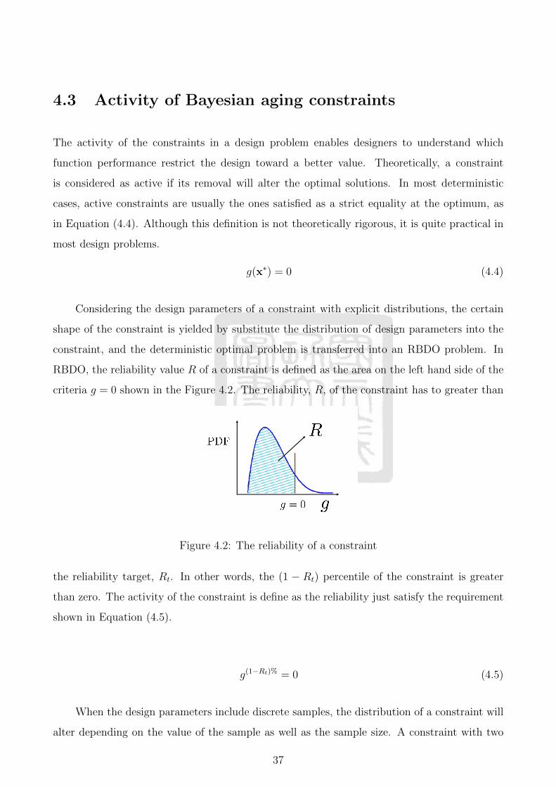
Considering the design parameters of a constraint with explicit distributions, the certain

shape of the constraint is yielded by substitute the distribution of design parameters into the

constraint, and the deterministic optimal problem is transferred into an RBDO problem. In

RBDO, the reliability value R of a constraint is defined as the area on the left hand side of the

criteria g = 0 shown in the Figure 4.2. The reliability, R, of the constraint has to greater than

Figure 4.2: The reliability of a constraint

the reliability target, Rt. In other words, the (1 − Rt) percentile of the constraint is greater

than zero. The activity of the constraint is define as the reliability just satisfy the requirement

shown in Equation (4.5).

g(1−Rt)% = 0 (4.5)

When the design parameters include discrete samples, the distribution of a constraint will

alter depending on the value of the sample as well as the sample size. A constraint with two

37

samples will result in two different probability density functions. Therefore, the reliability of a

constraint is not a constant anymore; a distribution instead. The original RBDO formulation

is then transferred into Bayesian RBDO that has the reliability as a distribution R. The form

of the constraint in Bayesian RBDO is the probability of the reliability, R, of the constraint

which is greater than target, Rt, is greater than a confidence range target, CRt. Therefore, we

can apply the same logic to calculate the reliability of the reliability , and set the activity of

the constraints as Equation(4.6):

R(1−CRt)% = Rt (4.6)

However, in the beta-binomial inference with sample points, the parameters of inferred reli-

ability distribution are discrete. Consequently, the area on the right hand side of reliability

target, called the confidence range, is also discrete. The same phenomenon is happened in

Poisson-gamma inference. The distribution parameters of the failure rate which is inferred

from Poisson-gamma inference are discontinuous. Due to the inferred distribution of the fail-

ure rate, the confidence range of aging process is also discrete. Therefore, a specific value of

confidence range target may not be able to be reached in both initial state and aging process.

Beside, the confidence ranges of the aging process do not have a closed form, we infer the con-

fidence ranges with MCMC that is giving a lot of samples to estimate the confidence ranges.

Therefore, the confidence ranges of aging process might not so accuracy do to the MCMC al-

gorithm. Considering these two reasons, we have to release the definition of activity. The new

definition of activity shows in Equation(4.7):

min(R(1−CR)% −Rt) (4.7)

There are two modified in Equation (4.7). First, Using the (1 − CR) percentile R instead of

applying (1 − CRt). The confidence ranges represent the degree of trust of these data, once

the confidence ranges satisfy the confidence target, they do not affect the following design

process; they serve as the thresholds. Furthermore, the specific confidence range target is not

available, the real confidence range, CR, is adapted to represent the truth. Then, in the general

case, the optimal design is right on the activity constraint. Taking the error form MCMC into

consideration, we release the definition of the activity; we just find the constraint which is

closest to optimal design.

38

4.4 Resource allocation of sample augmentation

When the confidence bounds do not exceed confidence target, adding new sample is needed. Due

to measuring takes time and cost, we want to just adding new samples on the most important

parameter. Therefore, before adding new sample, we should determine which parameter is the

most important to us. The strategy of adding new samples on critical parameter is shown in

the Figure 4.3

Yes

No

Figure 4.3: The strategy of adding new samples

After the first time optimization, we can yield the confidence ranges, CRR and CRf , in

the initial state and aging process. The constraint which has the lowest confidence ranges is

39

the critical constraint. If the critical constraint is the time-invariant, analyzing the sensitivity

on all sample parameters and set the most sensitive parameter as the critical parameter and

then adding new sample on the critical parameter in the initial state. However, if the critical

constraint is time variant, in order to get more information about failure rate, adding new

sample in the undetected time instant is required, hence, only the time-dependent parameters

are focused. The detail about sensitivity analysis and the algorithm of adding samples are

demonstrated in subsection 4.4.1 and 4.4.2.

Step 1 Define the constraint with the lowest confidence range as the critical constraint.

Step 2 Determine whether the critical constraint is a time-invariant constraint or not. If the

critical constraint is time-invariant, go to the step 3; otherwise, go to step 5.

Step 3 Find the critical sample parameter on the critical constraint by sensitivity analysis. If

the the critical constraint is the same as the previous iteration, we can simply adding new

samples on the critical parameter we yield in last iteration without executing sensitivity

analysis.

Step 4 Adding new samples on the critical parameter in the initial state with Markov chain

Monte Carlo (MCMC) Metropolis-Hastings algorithm. Go to the step 7.

Step 5 When the critical constraint is a time-variant constraint, we execute sensitivity analysis

on time-dependent parameters only. Find the critical time-dependent sample parameters.

Step 6 Adding new samples on the critical time-dependent parameter at undetected time

instant with Markov chain Monte Carlo (MCMC) Metropolis-Hastings algorithm. Adding

one sample on the critical time-dependent parameter means the time segments plus one.

Step 7 After adding new sample, return to update the optimization model to calculate the

updating confidence bounds and the confidence ranges. If the updating confidence bounds

still do not reach the confidence target, continuously adding new sample with this strategy.

40

4.4.1 Sensitivity analysis

In this thesis, we define the constraint with the lowest confidence range as the critical in

Bayesian optimization model. In order to rise the confidence range, adding new sample is

necessary. Before augment the sample size, We have to decide which parameter with sample

is the critical parameter. The critical parameter means the variation of the parameter would

lead to the most severe change on the constraint. We can decide the critical parameter by

analyzing sensitivity respect to each parameter in the critical constraint. The sensitivity of g

with respect to each parameter value is the derivative with respect to each parameter. Definition

of the sensitivity at the value of (y, z) shown in Equation(4.8):

sy =| ∂g∂y|y=y

sz =| ∂g∂z|z=z

(4.8)

where sy and sz are defined as sensitivity of parameter y and z.

Note that if the critical constraint is time variant, we analyze sensitivity of the critical

constraint with respect all the parameters in sample. On the other hand, when the critical

constraint is time variant, we just analyze the sensitivity on the time-dependent parameters

only.

4.4.2 MCMC bias sample filter

The estimation with bias samples might lead to inaccurate results; therefore, we have to use

Markov Chain Monte Carol (MCMC) (the Metropolis-Hastings algorithm is adopted in this

thesis) to avoid bias sample. MCMC is the method to generate a sequence of random samples

from a distribution and the Metropolis-Hastings algorithm is used to estimate the movement

tendency of the random sample within the filed of the distribution by calculating the acceptance

index of the next sample candidate xj. While calculating the acceptance index, the target

distribution and proposal distribution must be known. We obtain the target distribution by

use the statistic toolbox in commercial tool Matlab of existing samples, and the proposal

distribution is obtained by re-sampling technique of Bootstrap method. The Bootstrap method

41

is used to estimate a unknown underlying distribution with few current samples. In the initial

state, the size of current sample is n, and we can re-sample the current samples in the size n.

When the sets of re-sample set is large enough, we can use them to estimate the parameters of

underlying distribution.

The sequence of states constitutes a Markov chain with transition probability Pi,j as

Pi,j = q(i, j)ak(i, j), if j 6= i

Pi,i = q(i, i) +∑k 6=i

q(i, k)(1− ak(i, k))(4.9)

where q(i, j) is referred to as the proposal or candidate-generating distribution, represents that

when a process is at the point i, the density generates a value y from q(i, j). The Markov chain

Xn will be time reversible and have stationary probabilities π(j) if

π(i)Pi,j = π(j)Pj,i if j 6= i

π(i)q(i, j)ak(i, j) = π(j)q(j, i)ak(j, i)(4.10)

The ak(i; j), which is referred as the probability of move frome xi to xj,

ak(i, j) = min

(π(j)q(j, i)

π(i)q(i, j), 1

)(4.11)

If the acceptance index is greater than one, ak(i; j) ≥ 1; that means the probability of moving

from xi to xj is higher, and then we can set the xj as a new sample. In original concept of

Metropolis-Hasting, When the candidate xj of new sample is rejected, xi would be added again.

In the case of the critical constraint being time variant, getting new samples at an un-

detected time instance is desired. Adding a new sample that is the same as current sample

cannot help us learn more about the failure rate. Therefore, we have to draw an additional

sample with MCMC rejected samples until there exist an acceptable sample. Figure 4.4 shows

the flowchart of sample addition.

The procedure of the Metropolis-Hasting algorithm with arbitrary value s0 and our purpose

is to draw samples from target distribution :

1. Estimate statistical parameters of the underlying distribution by directly using existing

samples as target distribution π.

42

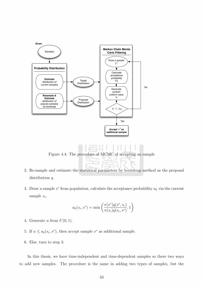
Samples

Given

Probability Distribution

Proposal Distribution

Resample & Estimate

distribution of pseudo-samples

by bootstrap

Target Distribution

Estimate distribution of

current samples

Markov Chain Monte Carlo Filtering

Draw a sample s∗

Accept s∗as additional sample

Yes

No

Calculate acceptance probability

ak

Generate random

uniform valueu

u < ak

Figure 4.4: The procedure of MCMC of accepting an sample

2. Re-sample and estimate the statistical parameters by bootstrap method as the proposal

distribution q.

3. Draw a sample s∗ from population, calculate the acceptance probability ak via the current

sample sc.

ak(sc, s∗) = min

(π(s∗)q(s∗, sc)

π(sc)q(sc, s∗), 1

)4. Generate u from U(0, 1).

5. If u ≤ ak(sc, s∗), then accept sample s∗ as additional sample.

6. Else, turn to step 3.

In this thesis, we have time-independent and time-dependent samples so there two ways

to add new samples. The procedure is the same in adding two types of samples, but the

43

ways to generate the target distribution and the proposal distribution are different. For time-

independent case, we just use the MATLAB toolbox fitting the current data in normal dis-

tributions and yield the target distribution, and use the concept of the Bootstrap to estimate

the proposal distribution. On the contrary, for the time-dependent case, we first the fitting

the samples that measured in the same time period, if we have three segments within a time

interval and we can yield three distributions, then get the modes of these three distributions,

finally, use the three modes to fit the target distribution of failure rate with MATLAB toolbox

. The way to generate the proposal distributions is much the same, but in the last step, we

re-sample the modes to infer the distribution of the failure rate with Bootstrap.

44

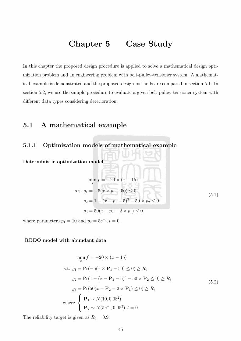
Chapter 5 Case Study

In this chapter the proposed design procedure is applied to solve a mathematical design opti-

mization problem and an engineering problem with belt-pulley-tensioner system. A mathemat-

ical example is demonstrated and the proposed design methods are compared in section 5.1. In

section 5.2, we use the sample procedure to evaluate a given belt-pulley-tensioner system with

different data types considering deterioration.

5.1 A mathematical example

5.1.1 Optimization models of mathematical example

Deterministic optimization model

minxf = −20× (x− 15)

s.t. g1 = −5(x× p1 − 50) ≤ 0

g2 = 1− (x− p1 − 5)3 − 50× p2 ≤ 0

g3 = 50(x− p2 − 2× p1) ≤ 0

(5.1)

where parameters p1 = 10 and p2 = 5e−t, t = 0.

RBDO model with abundant data

minxf = −20× (x− 15)

s.t. g1 = Pr(−5(x×P1 − 50) ≤ 0) ≥ Rt

g2 = Pr(1− (x−P1 − 5)3 − 50×P2 ≤ 0) ≥ Rt

g3 = Pr(50(x−P2 − 2×P1) ≤ 0) ≥ Rt

where

P1 ∼ N(10, 0.082)

P2 ∼ N(5e−t, 0.052), t = 0

(5.2)

The reliability target is given as Rt = 0.9.

45

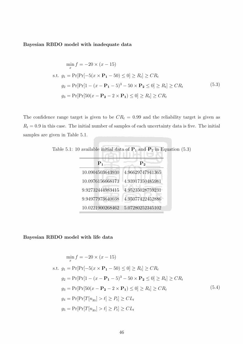
Bayesian RBDO model with inadequate data

minxf = −20× (x− 15)

s.t. g1 = Pr[Pr[−5(x×P1 − 50) ≤ 0] ≥ Rt] ≥ CRt

g2 = Pr[Pr[1− (x−P1 − 5)3 − 50×P2 ≤ 0] ≥ Rt] ≥ CRt

g3 = Pr[Pr[50(x−P2 − 2×P1) ≤ 0] ≥ Rt] ≥ CRt

(5.3)

The confidence range target is given to be CRt = 0.99 and the reliability target is given as

Rt = 0.9 in this case. The initial number of samples of each uncertainty data is five. The initial

samples are given in Table 5.1.

Table 5.1: 10 available initial data of P1 and P2 in Equation (5.3)

P1 P2

10.0904503643930 4.96629747941365

10.0976156668173 4.93917350485981

9.92732444983415 4.95235028759231

9.94977973640038 4.95077422452886

10.0221900268462 5.07280252345102

Bayesian RBDO model with life data

minxf = −20× (x− 15)

s.t. g1 = Pr[Pr[−5(x×P1 − 50) ≤ 0] ≥ Rt] ≥ CRt

g2 = Pr[Pr[1− (x−P1 − 5)3 − 50×P2 ≤ 0] ≥ Rt] ≥ CRt

g3 = Pr[Pr[50(x−P2 − 2×P1) ≤ 0] ≥ Rt] ≥ CRt

g4 = Pr[Pr[T [ng2 ] > t] ≥ Pt] ≥ CLt

g5 = Pr[Pr[T [ng3 ] > t] ≥ Pt] ≥ CLt

(5.4)

46

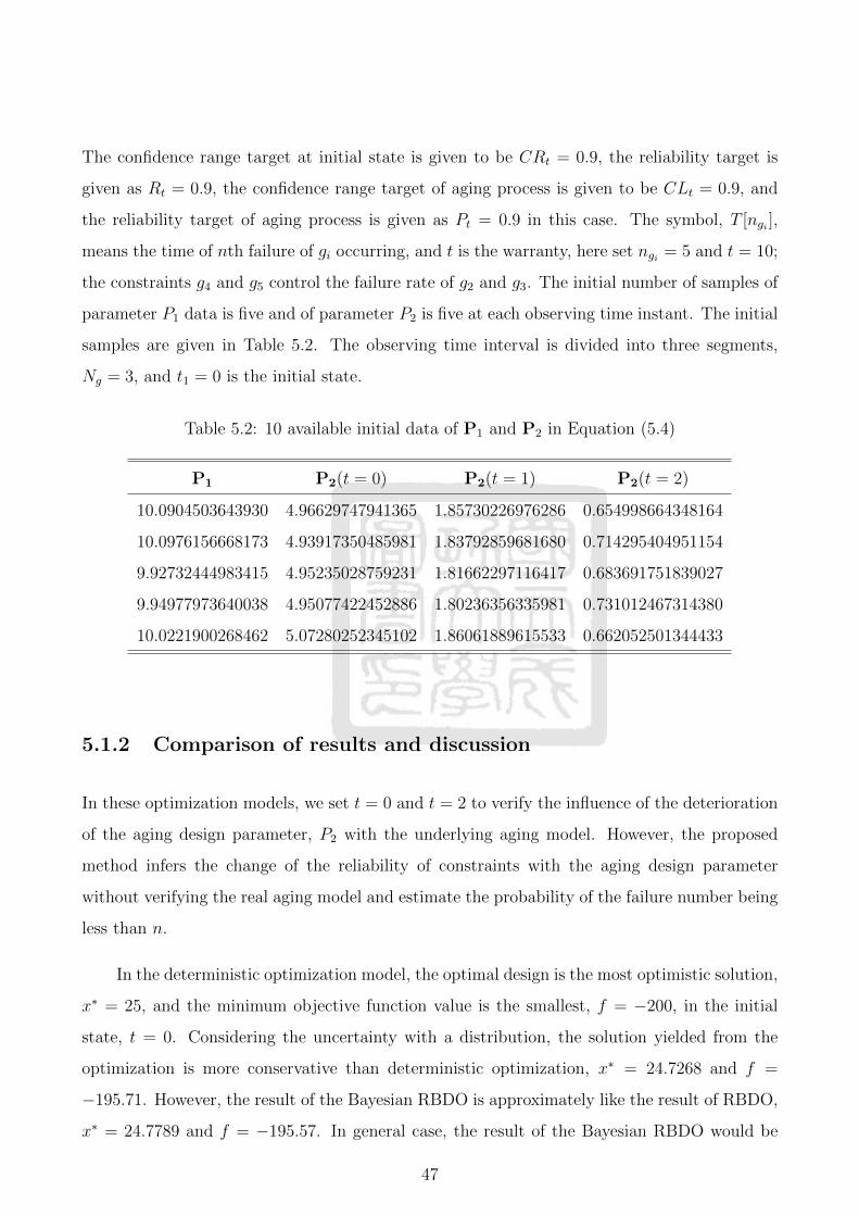
The confidence range target at initial state is given to be CRt = 0.9, the reliability target is

given as Rt = 0.9, the confidence range target of aging process is given to be CLt = 0.9, and

the reliability target of aging process is given as Pt = 0.9 in this case. The symbol, T [ngi ],

means the time of nth failure of gi occurring, and t is the warranty, here set ngi = 5 and t = 10;

the constraints g4 and g5 control the failure rate of g2 and g3. The initial number of samples of

parameter P1 data is five and of parameter P2 is five at each observing time instant. The initial

samples are given in Table 5.2. The observing time interval is divided into three segments,

Ng = 3, and t1 = 0 is the initial state.

Table 5.2: 10 available initial data of P1 and P2 in Equation (5.4)

P1 P2(t = 0) P2(t = 1) P2(t = 2)

10.0904503643930 4.96629747941365 1.85730226976286 0.654998664348164

10.0976156668173 4.93917350485981 1.83792859681680 0.714295404951154

9.92732444983415 4.95235028759231 1.81662297116417 0.683691751839027

9.94977973640038 4.95077422452886 1.80236356335981 0.731012467314380

10.0221900268462 5.07280252345102 1.86061889615533 0.662052501344433

5.1.2 Comparison of results and discussion

In these optimization models, we set t = 0 and t = 2 to verify the influence of the deterioration

of the aging design parameter, P2 with the underlying aging model. However, the proposed

method infers the change of the reliability of constraints with the aging design parameter

without verifying the real aging model and estimate the probability of the failure number being

less than n.

In the deterministic optimization model, the optimal design is the most optimistic solution,

x∗ = 25, and the minimum objective function value is the smallest, f = −200, in the initial

state, t = 0. Considering the uncertainty with a distribution, the solution yielded from the

optimization is more conservative than deterministic optimization, x∗ = 24.7268 and f =

−195.71. However, the result of the Bayesian RBDO is approximately like the result of RBDO,

x∗ = 24.7789 and f = −195.57. In general case, the result of the Bayesian RBDO would be

47

more conservative than of RBDO, but the result could be influence by the quality of samples.

Therefore, the result of Bayesian RBDO has a chance being more optimistic than RBDO.

Taking deterioration into consideration, the Bayesian RBDO is transferred into time-dependent

Bayesian RBDO. In order to control the failure number being less than 5 while t ∈ [0, 2],

the result of the time-dependent Bayesian RBDO is dramatically shifted, x∗ = 20.4713 and

f = −109.4257. In fact, in this mathematical example, the underlying aging process is the

exponential decay. We set the time, t = 2, the aging parameter affects the performance of these

constraint, therefore, the optimal design of deterministic is shift, x∗ = 20.676 and f = −113.533.

The optimal design of RBDO at t = 2 is yielded, x∗ = 20.4017 and f = −109.270, and the

optimal design of Bayesian RBDO at t = 2 is obtained, x∗ = 20.4595 and f = −110.8951.

The assumption is slightly difference between time-dependent Bayesian RBDO and others.

The requirements of time-dependent Bayesian RBDO is the number of failure being less than

5 within t ∈ [0, 2]. However, the requirement of RBDO and Bayesian RBDO is the probability

of failure at t = 2 is less than Rt. This two requirements would be transferred to another, the

product of the size of the the population and the probability of failure is the number of failure.

By assuming the size of the population is a hundred, and the limited number of failure is five,

therefore, the failure probability is R = 0.95. The target reliability is set as Rt = 0.95 in the

RBDO and Bayesian RBDO optimization at t = 2.

Compared with the results at t = 2 the result of the time-dependent Bayesian RBDO, the

result of the results of RBDO, Bayesian RBDO, and time-dependent Bayesian RBDO are quit

similar. We can use these aging data to predict the aging process without inferring the true

aging model and yield a acceptable result.

5.1.3 Summary

This proposed method could infer the aging process without inferring the true model of aging

process. The result yielded from the time-dependent Bayesian RBDO is not the conservative

one, because the assumption is slightly different and the inferring process involves the random

process. However, the time-dependent Bayesian RBDO could deal with the aging process and

yield a reasonable result.

48

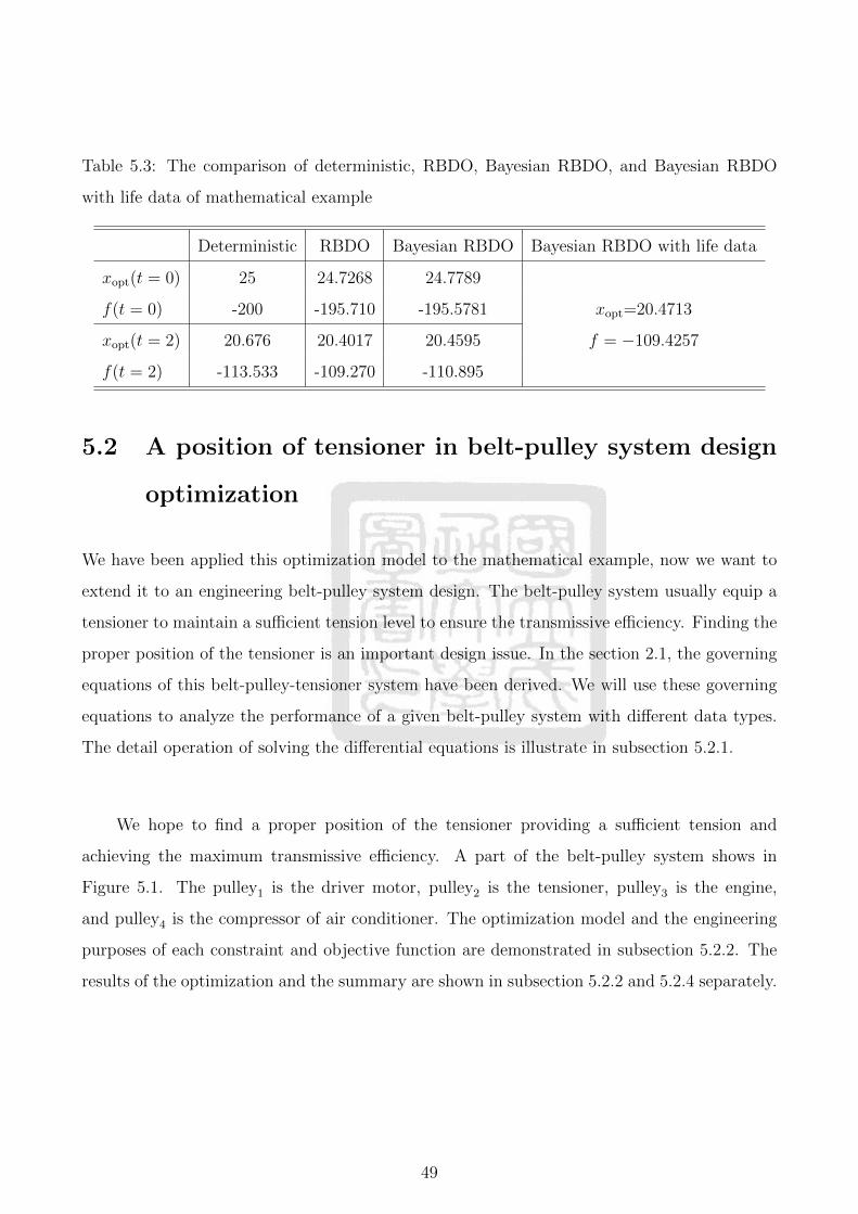
Table 5.3: The comparison of deterministic, RBDO, Bayesian RBDO, and Bayesian RBDO

with life data of mathematical example

Deterministic RBDO Bayesian RBDO Bayesian RBDO with life data

xopt(t = 0) 25 24.7268 24.7789

f(t = 0) -200 -195.710 -195.5781 xopt=20.4713

xopt(t = 2) 20.676 20.4017 20.4595 f = −109.4257

f(t = 2) -113.533 -109.270 -110.895

5.2 A position of tensioner in belt-pulley system design

optimization

We have been applied this optimization model to the mathematical example, now we want to

extend it to an engineering belt-pulley system design. The belt-pulley system usually equip a

tensioner to maintain a sufficient tension level to ensure the transmissive efficiency. Finding the

proper position of the tensioner is an important design issue. In the section 2.1, the governing

equations of this belt-pulley-tensioner system have been derived. We will use these governing

equations to analyze the performance of a given belt-pulley system with different data types.

The detail operation of solving the differential equations is illustrate in subsection 5.2.1.

We hope to find a proper position of the tensioner providing a sufficient tension and

achieving the maximum transmissive efficiency. A part of the belt-pulley system shows in

Figure 5.1. The pulley1 is the driver motor, pulley2 is the tensioner, pulley3 is the engine,

and pulley4 is the compressor of air conditioner. The optimization model and the engineering

purposes of each constraint and objective function are demonstrated in subsection 5.2.2. The

results of the optimization and the summary are shown in subsection 5.2.2 and 5.2.4 separately.

49

Figure 5.1: Two pulleys belt system

5.2.1 Numerical adjustment of belt-pulley system

The two basic governing in span zone is shown in Equation5.5a.

(T −GV )′ + EIκκ′ = 0

(T −GV )κ− EIκ′′ = 0

From Equation 2.5, Let T − GV = W and we can yield three differential equations. For

geometric requirements, other four differential equations are yielded. The s is the length of the

span, 0 ≥ s ≥ L

• Physical differential equations:

– dW/ds = EIκκ′, derived from Equation(5.5a).

– dκ/ds = W/κ× EI, derived from Equation(5.5a).

– d2κ/ds2 = Wκ/EI, derived from Equation(5.5a).

• Geometric differential equations:

50

– dθ/ds = κ, it is the definition of curvature.

– dx/ds = cos θ, x is a position on x-axis.

– dy/ds = sin θ, y is a position on y-axis.

– dL/ds = 0, L is the length of span in steady motion and it is a constant.

Some boundary conditions are needed to solve the physical and geometric differential equations.

These boundaries are there to ensure the belt exactly contacts with pulleys and they are

orthogonal at the points of contacts.

• Boundary conditions:

– W (0) = T (0)−GV (0), the initial value of span closed to pulleyi

– κ(0) = 1/Ri, at points of contacts, the curvature of belt is equal to which of pulleys.

– κ(L) = 1/Ri+1

– x(0) = Ri sin(θ(0)), ensuring the belt is orthogonal to pulleys.

– x(L)−Di = Ri+1 sin(θ(L))

– x(0)2 + y(0)2 = Ri, ensuring the belt contact with pulleys.

– x(L)−D2i + y(L)2 = Ri+1

There is a problem when solving these differential equations, the length of the span L is

unknown. We can solve this problem by setting these variables non-dimensional, s = s/L,

x = x/L, y = y/L, κ = κL, and W = WL2/EI. After this operation, the ranges of s is

normalized to 0 ≥ s ≥ 1 Substitute these non-dimensional variables into seven differential and

boundary conditions yields:

• Physical differential equations:

– dW/ds = κκ′

– dκ/ds = −W/κ

– d2κ/ds2 = W κ

• Geometric differential equations:

51

– dθ/ds = κ

– dx/ds = cos θ

– dy/ds = sin θ

– dL/ds = 0

• Boundary conditions:

– ˆW (0) = W (0)L2/EI, the initial value of span closed to pulleyi

– ˆκ(0) = L/Ri, at points of contacts, the curvature of belt is equal to which of pulleys.

– κ(1) = L/Ri+1

– L(0)x(0) = Ri sin(θ(0)), ensuring the belt is orthogonal to pulleys.

– Lx(1)−Di = Ri+1 sin(θ(L))

– Lx(0)2 + Ly(0)2 = Ri, ensuring the belt contact with pulleys.

– Lx(1)−D2i + Ly(1)2 = Ri+1

After non-dimensional operation, these seven differential equations are transferred into the

standard boundary value problem(BVP). We can solve them by BVP solver, and obtain the

solution about W , θ, κ, κ′,L, x and y. In this thesis, we choose bvp4c as the solver in MATLAB

toolbox. When using the bvp4c, the numerical initial values are required for each parameter.

The improper initial values would lead a wrong results. The most unpredictable initial value is

the length of span in the steady motion, L. In order to proceed to the optimization, the initial

value of L has to be generate automatically. This initial value generator guess an initial value

based on the distance between two pulleys. However, this generator does not work properly at

each iteration, and the initial value of each iteration might change. To ensure the optimization

work well, therefore, we display the maximum residual in the solving process and demand the

residual is less the 0.1%, or re-solve the BVP with other initial values until the maximum

residual satisfy the requirement.

5.2.2 The design model of belt-pulley systems

The properties of the belt such as bending stiffness, EI, the longitudinal stiffness, EA, and

the fluctuation of radius of pulleys would influence the performance of the belt-pulley system

52

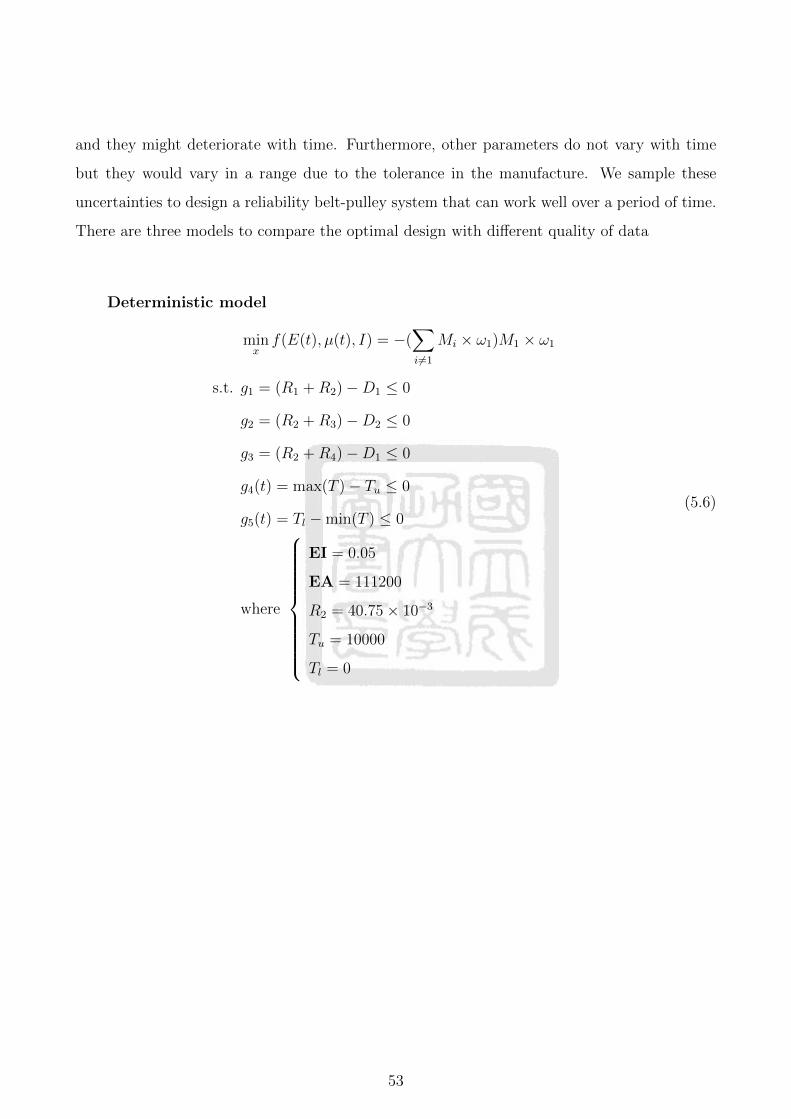
and they might deteriorate with time. Furthermore, other parameters do not vary with time

but they would vary in a range due to the tolerance in the manufacture. We sample these

uncertainties to design a reliability belt-pulley system that can work well over a period of time.

There are three models to compare the optimal design with different quality of data

Deterministic model

minxf(E(t), µ(t), I) = −(

∑i 6=1

Mi × ω1)M1 × ω1

s.t. g1 = (R1 +R2)−D1 ≤ 0

g2 = (R2 +R3)−D2 ≤ 0

g3 = (R2 +R4)−D1 ≤ 0

g4(t) = max(T )− Tu ≤ 0

g5(t) = Tl −min(T ) ≤ 0

where

EI = 0.05

EA = 111200

R2 = 40.75× 10−3

Tu = 10000

Tl = 0

(5.6)

53

RBDO model

minxf(E(t), µ(t), I) = −(

∑i 6=1

Mi × ωi)/M1 × ω1

s.t. g1 = Pr((R1 +R2)−D1 ≤ 0) ≥ Rt

g2 = Pr((R2 +R3)−D2 ≤ 0) ≥ Rt

g3 = Pr((R2 +R4)−D1 ≤ 0) ≥ Rt

g4(t) = Pr(max(T )− Tu ≤ 0) ≥ Rt

g5(t) = Pr(Tl −min(T ) ≤ 0) ≥ Rt

where

EI ∼ N(0.05, 0.005)

EA ∼ N(111200, 100)

R2 ∼ N(40.75× 10−3, 0.8)

Tu = 10000, Tl = 0

Rt = 0.8

(5.7)

Bayesian RBDO model with life data

minxf(E(t), µ(t), I) = −(

∑i 6=1

Mi × ω1)M1 × ω1

s.t. g1 = Pr(Pr((R1 +R2)−D1 ≤ 0) ≥ Rt) ≥ CRt

g2 = Pr(Pr((R2 +R3)−D2 ≤ 0) ≥ Rt) ≥ CRt

g3 = Pr(Pr((R2 +R4)−D1 ≤ 0) ≥ Rt) ≥ CRt

g4(t) = Pr(Pr(max(T )− Tu ≤ 0) ≥ Rt) ≥ CRt

g5(t) = Pr(Pr(Tl −min(T ) ≤ 0) ≥ Rt) ≥ CRt

g6 = Pr(Pr(T [ng4 ] > t) ≥ Pt) ≥ CLt

g7 = Pr(Pr(T [ng5 ] > t) ≥ Pt) ≥ CLt

where

Tu = 10000, Tl = 0

Rt = 0.8, CRt = 0.8andCLt = 0.8

ng4 , ng5 = 3

t = 10

(5.8)

The first to third constraints in three models ensure the tensioner does not contact with

pulleys and the fourth and fifth constraints are the maximum and minimum tension require-

ments. Furthermore, the sixth and seventh constraints in the Bayesian RBDO model govern

54

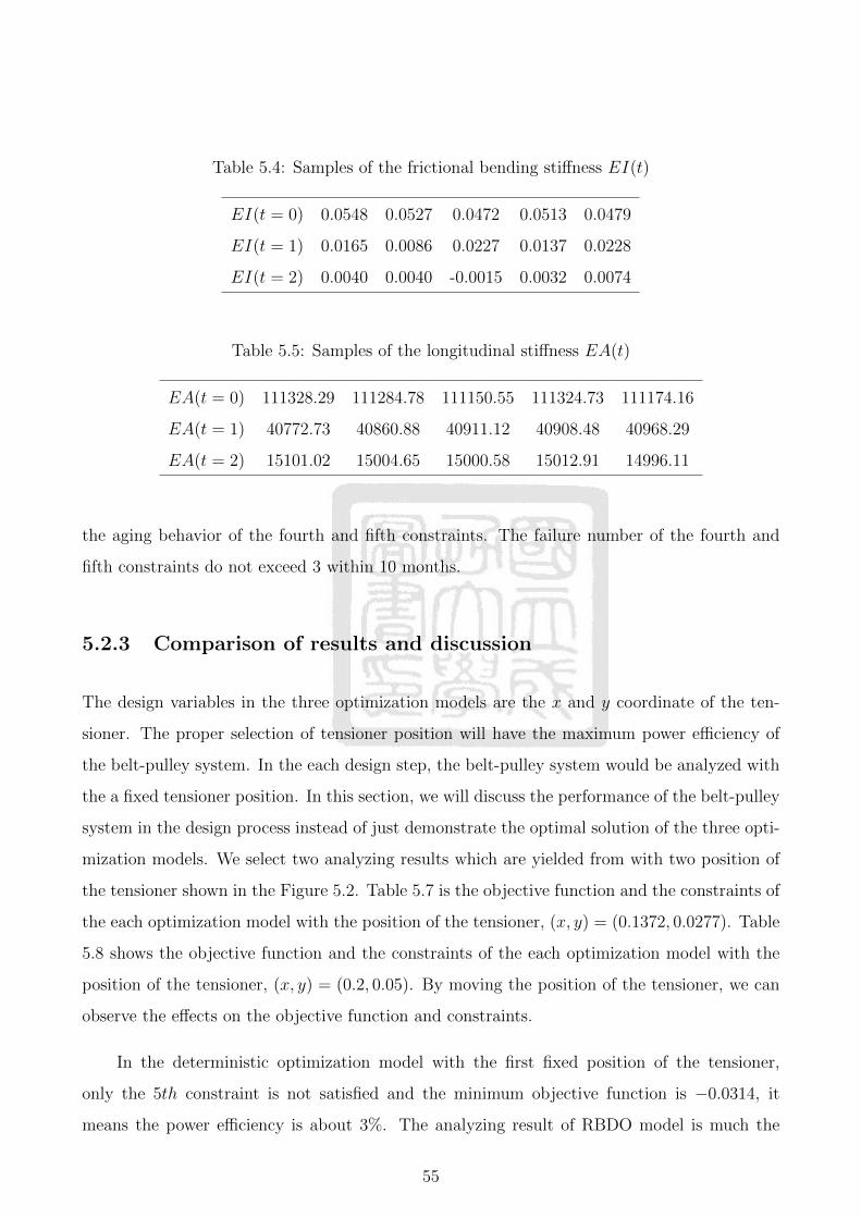
Table 5.4: Samples of the frictional bending stiffness EI(t)

EI(t = 0) 0.0548 0.0527 0.0472 0.0513 0.0479

EI(t = 1) 0.0165 0.0086 0.0227 0.0137 0.0228

EI(t = 2) 0.0040 0.0040 -0.0015 0.0032 0.0074

Table 5.5: Samples of the longitudinal stiffness EA(t)

EA(t = 0) 111328.29 111284.78 111150.55 111324.73 111174.16

EA(t = 1) 40772.73 40860.88 40911.12 40908.48 40968.29

EA(t = 2) 15101.02 15004.65 15000.58 15012.91 14996.11

the aging behavior of the fourth and fifth constraints. The failure number of the fourth and

fifth constraints do not exceed 3 within 10 months.

5.2.3 Comparison of results and discussion

The design variables in the three optimization models are the x and y coordinate of the ten-

sioner. The proper selection of tensioner position will have the maximum power efficiency of

the belt-pulley system. In the each design step, the belt-pulley system would be analyzed with

the a fixed tensioner position. In this section, we will discuss the performance of the belt-pulley

system in the design process instead of just demonstrate the optimal solution of the three opti-

mization models. We select two analyzing results which are yielded from with two position of

the tensioner shown in the Figure 5.2. Table 5.7 is the objective function and the constraints of

the each optimization model with the position of the tensioner, (x, y) = (0.1372, 0.0277). Table

5.8 shows the objective function and the constraints of the each optimization model with the

position of the tensioner, (x, y) = (0.2, 0.05). By moving the position of the tensioner, we can

observe the effects on the objective function and constraints.

In the deterministic optimization model with the first fixed position of the tensioner,

only the 5th constraint is not satisfied and the minimum objective function is −0.0314, it

means the power efficiency is about 3%. The analyzing result of RBDO model is much the

55

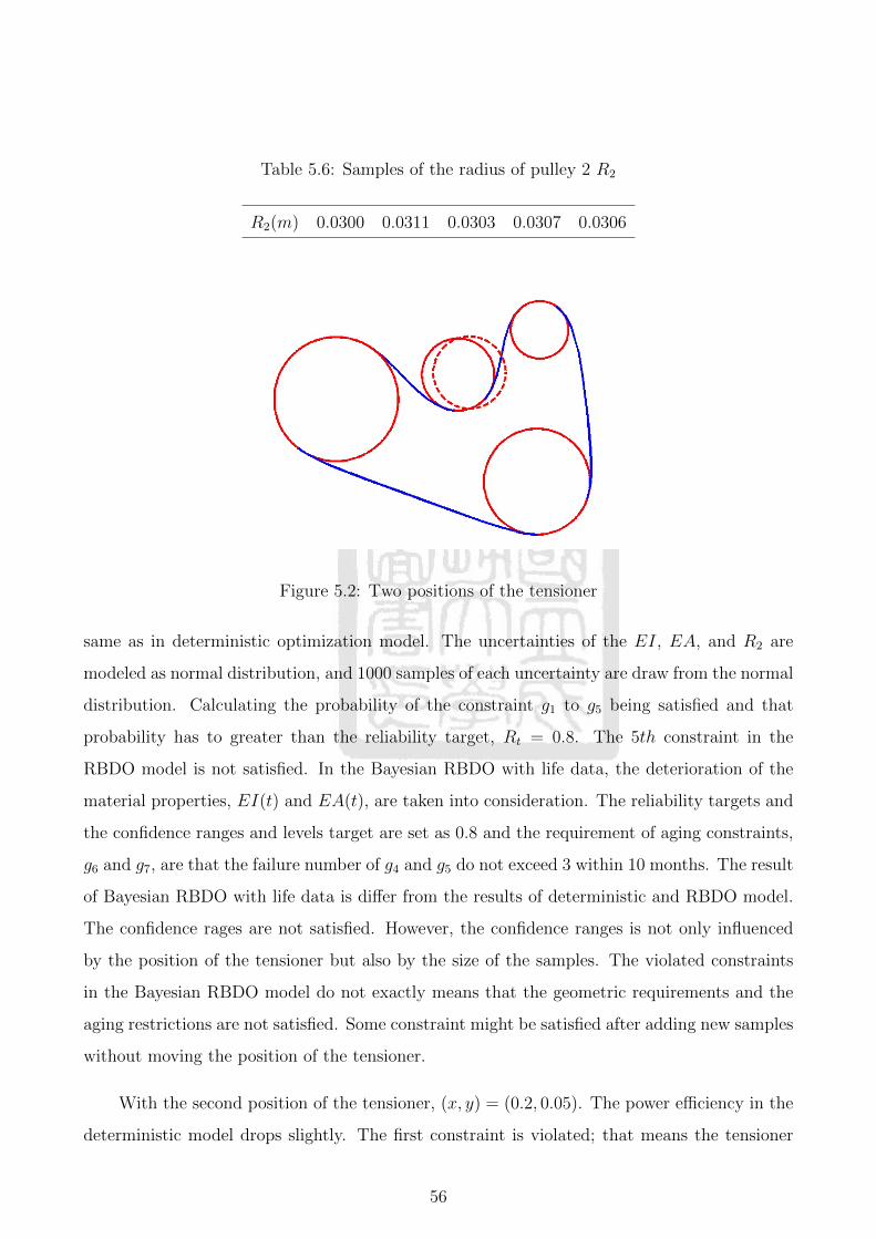
Table 5.6: Samples of the radius of pulley 2 R2

R2(m) 0.0300 0.0311 0.0303 0.0307 0.0306

Figure 5.2: Two positions of the tensioner

same as in deterministic optimization model. The uncertainties of the EI, EA, and R2 are

modeled as normal distribution, and 1000 samples of each uncertainty are draw from the normal

distribution. Calculating the probability of the constraint g1 to g5 being satisfied and that

probability has to greater than the reliability target, Rt = 0.8. The 5th constraint in the

RBDO model is not satisfied. In the Bayesian RBDO with life data, the deterioration of the

material properties, EI(t) and EA(t), are taken into consideration. The reliability targets and

the confidence ranges and levels target are set as 0.8 and the requirement of aging constraints,

g6 and g7, are that the failure number of g4 and g5 do not exceed 3 within 10 months. The result

of Bayesian RBDO with life data is differ from the results of deterministic and RBDO model.

The confidence rages are not satisfied. However, the confidence ranges is not only influenced

by the position of the tensioner but also by the size of the samples. The violated constraints

in the Bayesian RBDO model do not exactly means that the geometric requirements and the

aging restrictions are not satisfied. Some constraint might be satisfied after adding new samples

without moving the position of the tensioner.

With the second position of the tensioner, (x, y) = (0.2, 0.05). The power efficiency in the

deterministic model drops slightly. The first constraint is violated; that means the tensioner

56

Table 5.7: The analysis of the belt-pulley system with fixed position of tensioner (x, y) =

(0.1372, 0.0277)

Models Objective function Constraints

Deterministic -0.03256 (-0.0314,-0.0292,-0.0493,-9312.5,1608.5)

RBDO -0.03263 (-0.2,-0.2,-0.2,-0.16,0.8)

Bayesian RBDO with life data -0.0629 (0.0776,0.0776,0.0776,0.999,0.876,0.999,-0.243)

Table 5.8: The analysis of the belt-pulley system with fixed position of tensioner (x, y) =

(0.2, 0.05)

Models Objective function Constraints

Deterministic -0.03251 (0.0329,-0.0954,-0.0448,-10858,0)

RBDO -0.03249 (0.8,-0.2,-0.2,-0.2,-0.2)

Bayesian RBDO with life data 0 (0.999,0.0776,0.0776,0.999,0.0777,0.999,-0.243)

interferes with pulleys. However, the maximum and minimum tension requirements are satisfied

in this case. The minimum tension changes a lot with the position of the tensioner in the

deterministic model. The result of RBDO model shows that the tensioner interferes with the

pulley and the fifth constraint now is satisfied, and the value of objective function drop slightly

too. The result of the Bayesian RBDO model has a similar tendency to deterministic and

RBDO model, the constraints g1 and g5 is influenced most by the change of the position of the

tensioner. However, the position of the tensioner does not influence the aging behavior greatly.

In the Bayesian RBDO model, the aging process is estimated by the total failure number over a

period of time and the number of subsection of time. The movement of the tensioner influence

the total failure number only.

57

5.2.4 Summary

Overall, we have the following observations using the proposed method in the belt-pulley sys-

tem.

1. With a fixed position of the tensioner, the result of the Bayesian RBDO might be influ-

enced by the biased sample.

2. The aging constraints are not affected greatly by the change of the position of the ten-

sioner.

3. In this belt-pulley system, the position of the tensioner influence the tension of the belt

greatly.

The tension of the belt would influence the performance of the system. Therefore, we can choose

a proper position of the tensioner to achieve the maximum efficiency of belt-pulley system.

58

Chapter 6 Conclusion and Future Work

6.1 Conclusion

The main purpose of this thesis is to propose a design method considering the deterioration of

components to address the time-dependent reliability-based design optimization with life data

and satisfy the confidence and reliability targets.

In Chapter 3, the selection of the priors in the Bayesian inference is specified, and esti-

mation of reliability of a constraints using Bayesian inference with life data is constructed and

definition of the confidence ranges and confidence bounds is done. In Chapter 4, the overall de-

sign scheme is proposed. In this design scheme, the fewest additional sample is required. When

adding new sample is necessary, the strategy of adding new samples is proposed based on the

types of the constraints and the importance of the parameters. In Chapter 5, a mathematical

example and a belt-pulley design show the validity of proposed design scheme.

Three main contributions of this thesis:

1. Use the fewest number of sample to satisfy the confidence target and yield

a optimal design under the confidence and reliability targets: The additional

sample is added to satisfy the lowest confidence target and in the design process, the

optimization algorithm would force the design to satisfy the reliability target. If the

reach the reliability target is impossible, the proposed method would tell the user there

are no feasible solution with current size of sample.

2. Allocate the resource to improve the confidence more efficiently: The measure-

ments of sample is expensive, therefore, the critical parameter is the only focus. For

time-variant constraint, determine the critical parameter by analyzing the sensitivity of

the time-dependent parameter; for time-invariant constraints, analyze the sensitivity of

all parameters, and define the most sensitive parameter as the critical parameter.

3. Make the BVP solver more steady while optimization: The optimization pro-

cess would be terminated by encountering the singular point while solving the BVP. We

59

construct a initial value generator to choose a proper initial value to avoid the singular

points. While encounter the singular points, we force the optimization process continue,

but the ill solution will be excluded.

6.2 Future work

There are some points deserving further investigation:

1. The strategy of modifying the reliability targets, while the optimization target can not

be satisfy under current size of samples.

2. The impact of sample on objective function. In this thesis, we simply minimize the

maximum objective function value, but the approach might lead too strict result.

3. Taking censor data into consideration. The censor data with no exact failure time and

value need other way to analyze them and include them in the design method.

60

References

[1] R. C. Juvinall and K. M. Marshek, Fundamentals of Machine Component Design. John

Wiley and Sons Pte Ltd, 4th ed., 2006.

[2] E.-Y. Chu, “Fatigue test and stress analysis of v-belt,” Master’s thesis, National Cheng

Kung University, Tainan, Taiwan, 2007.

[3] T. C. Firbank, “Mechanics of the belt drive,” International Journal of Mechanical Sciences,

vol. 12, pp. 1053–1063, 1970.

[4] G. Gerbert, “Belt slip—a unified approach,” Journal of Mechanical Design, vol. 118,

pp. 432–438, 1996.

[5] D. G. Alciatore and A. E. Traver, “Multi-pulley belt drive mechanics : Creep theory v.s

shear theory,” Journal of Mechanical Design, vol. 117, pp. 506–511, 1995.

[6] S. E. Bechtel, S. Vohra, K. I. Jacob, and C. D. Carlson, “The stretching and slipping of

belts and fibers on pulleys,” Journal of Mechanical Design, vol. 67, pp. 197–206, 2000.

[7] M. B. Rubin, “An exact solution for steady motion of an extensible belt in multi-pulley

belt drive systems,” Journal of Mechanical Design, vol. 122, pp. 311–316, 2000.

[8] R. G. Parker and L. Kong., “Mechanics of serpentine belt drives with tensioner assemblies

and belt bending stiffness,” Journal of Mechanical Design, vol. 127, pp. 957–966, 2005.

[9] R. G. Parker and L. Kong., “Steady mechanics of belt-pulley systems,” Journal of Me-

chanical Design, vol. 27, pp. 25–34, 2005.

[10] X. Du, A. Sudjianto, and B. Huang, “Reliability-based design with the mixture of random

and interval variables,” Journal of Mechanical Design, vol. 127, pp. 1068–1076, 2005.

[11] D. Athow and J. Law, “Development and application of a random variable model for cold

load pickup,” IEEE Transactions on Power Delivery, vol. 9, pp. 1647–1653, 1994.

[12] G. Feng, “Eye movement as time-series random variables: A stochastic model of eye

movement control in leading,” Cognitive System Research, vol. 7, pp. 70–95, 2006.

61

[13] M. Hohenbichler and R. Rackwitz, “First-order concepts in system reliability,” Structural

Safety, vol. 1, no. 3, pp. 177–188, 1983.

[14] Y. Zhao and T. Ono, “A general procedure for first/second-order reliability method (FOR-

M/SORM),” Structural Safety, vol. 21, no. 2, pp. 95–112, 1999.

[15] A. Chiralaksanakul and S. Mahadevan, “First-order approximation methods in reliability-

based design optimization,” Journal of Mechanical Design, vol. 127, p. 851, 2005.

[16] S. Au and J. Beck, “A new adaptive importance sampling scheme for reliability calcula-

tions,” Structural Safety, vol. 21, no. 2, pp. 135–158, 1999.

[17] Y. Wu, H. Millwater, and T. Cruse, “Advanced probabilistic structural analysis method

for implicit performance functions,” AIAA journal, vol. 28, no. 9, pp. 1663–1669, 1990.

[18] K. Choi and B. Youn, “Hybrid analysis method for reliability-based design optimization,”

in 27th ASME Design Automation Conference, pp. 9–12, 2001.

[19] X. Du and W. Chen, “Sequential optimization and reliability assessment method for effi-

cient probabilistic design,” Journal of Mechanical Design, vol. 126, pp. 225–233, 2004.

[20] J. Liang, Z. Mourelatos, and J. Tu, “A single-loop method for reliability-based design

optimization,” International Journal of Product Development, vol. 5, no. 1, pp. 76–92,

2008.

[21] X. Du, A. Sudjianto, and W. Chen, “An integrated framework for optimization under

uncertainty using inverse reliability strategy,” Journal of Mechanical Design, vol. 126,

p. 562, 2004.

[22] S. Rahman and H. Xu, “A univariate dimension-reduction method for multi-dimensional

integration in stochastic mechanics,” Probabilistic Engineering Mechanics, vol. 19, no. 4,

pp. 393–408, 2004.

[23] I. Lee, K. Choi, L. Du, and D. Gorsich, “Dimension reduction method for reliability-based

robust design optimization,” Computers and Structures, vol. 86, no. 13-14, pp. 1550–1562,

2008.

62

[24] Z. Zong and K. Lam, “Bayesian estimation of complicated distributions,” Structural Safety,

vol. 22, no. 1, pp. 81–95, 2000.

[25] Z. Zong and K. Lam, “Bayesian estimation of 2-dimensional complicated distributions,”

Structural Safety, vol. 23, no. 2, pp. 105–121, 2001.

[26] V. Picheny, N. Kim, and R. Haftka, “Application of bootstrap method in conservative esti-

mation of reliability with limited samples,” Structural and Multidisciplinary Optimization,

vol. 41, no. 2, pp. 205–217, 2010.

[27] L. Du, K. Choi, and B. Youn, “Inverse possibility analysis method for possibility-based

design optimization,” AIAA journal, vol. 44, no. 11, pp. 2682–2690, 2006.

[28] L. Du and K. Choi, “An inverse analysis method for design optimization with both sta-

tistical and fuzzy uncertainties,” Structural and Multidisciplinary Optimization, vol. 37,

no. 2, pp. 107–119, 2008.

[29] C. Spetzler and C. Von Holstein, “Probability encoding in decision analysis,” Management

Science, vol. 22, pp. 340–358, 1975.

[30] L. Utkin and S. Gurov, “A general formal approach for fuzzy reliability analysis in the

possibility context,” Fuzzy Sets and Systems, vol. 83, no. 2, pp. 203–213, 1996.

[31] X. Bai and S. Asgarpoor, “Fuzzy-based approaches to substation reliability evaluation,”

Electric Power Systems Research, vol. 69, no. 2, pp. 197–204, 2004.

[32] L. Du, K. Choi, B. Youn, and D. Gorsich, “Possibility-based design optimization method

for design problems with both statistical and fuzzy input data,” Journal of Mechanical

Design, vol. 128, p. 928, 2006.

[33] J. Zhou and Z. Mourelatos, “A sequential algorithm for possibility-based design optimiza-

tion,” Journal of Mechanical Design, vol. 130, p. 011001, 2008.

[34] B. Youn, K. Choi, L. Du, and D. Gorsich, “Integration of possibility-based optimization

and robust design for epistemic uncertainty,” Journal of Mechanical Design, vol. 129,

p. 876, 2007.

63

[35] Z. Mourelatos and J. Zhou, “Design optimization under uncertainty using evidence theory,”

Reliability and Robust Design in Automotive Engineering, vol. 2032, p. 99, 2006.

[36] K. Sentz and S. Ferson, Combination of Evidence in Dempster-Shafer theory. Sandia

National Laboratories, California: Sandia National Laboratories, 2002.

[37] H. Bae, R. Grandhi, and R. Canfield, “Uncertainty quantification of structural response

using evidence theory,” AIAA journal, vol. 41, no. 10, pp. 2062–2068, 2003.

[38] J. Helton, J. Johnson, W. Oberkampf, and C. Sallaberry, “Sensitivity analysis in conjunc-

tion with evidence theory representations of epistemic uncertainty,” Reliability Engineering

and System Safety, vol. 91, no. 10, pp. 1414–1434, 2006.

[39] S. Gunawan and P. Papalambros, “A bayesian approach to reliability-based optimization

with incomplete information,” Journal of Mechanical Design, vol. 128, no. 4, pp. 900–918,

2006.

[40] B. Youn and P. Wang, “Bayesian reliability-based design optimization using eigenvector

dimension reduction (edr) method,” Structural and Multidisciplinary Optimization, vol. 36,

no. 2, pp. 107–123, 2008.

[41] J. Choi, D. An, and J. Won, “Bayesian approach for structural reliability analysis and op-

timization using the kriging dimension reduction method,” Journal of Mechanical Design,

vol. 132, p. 051003, 2010.

[42] R. Zhang and S. Mahadevan, “Model uncertainty and bayesian updating in reliability-

based inspection,” Structural Safety, vol. 22, no. 2, pp. 145–160, 2000.

[43] F. Coolen and M. Newby, “Bayesian reliability analysis with imprecise prior probabilities,”

Reliability Engineering & System Safety, vol. 43, no. 1, pp. 75–85, 1994.

[44] H. Huang, M. Zuo, and Z. Sun, “Bayesian reliability analysis for fuzzy lifetime data,”

Fuzzy Sets and Systems, vol. 157, pp. 1674–1686, 2006.

[45] P. Wang, B. Youn, Z. Xi, and A. Kloess, “Bayesian reliability analysis with evolving,

insufficient, and subjective data sets,” Journal of Mechanical Design, vol. 131, p. 111008,

2009.

64

[46] T. I. R. Alzbutas, “Application of bayesian methods for age-dependent reliability analysis,”

Quality and Reliability Engineering International, vol. doi: 10.1002/qre.1482, 2013.

[47] Z. Wang and P. Wang, “Reliability-based product design with time-dependent performance

deterioration,” in Prognostics and Health Management (PHM), 2012 IEEE Conference on,

pp. 1–12, 2012.

[48] Z. Hu, H. Li, X. Du, and K. Chandrashekhara, “Simulation-based time-dependent reliabil-

ity analysis for composite hydrokinetic turbine blades,” Structural and Multidisciplinary

Optimization, vol. 47, no. 5, pp. 765–781, 2013.

[49] A. Singh, Z. P. Mourelatos, and J. Li, “Design for lifecycle cost using time-dependent

reliability,” Journal of Mechanical Design, vol. 132, p. 091008, 2010.

[50] A. G. Colombo, “Bayes nonparametric estimation of time-dependent failure rate,” Relia-

bility, IEEE Transactions on, vol. 34, pp. 109–112, 1985.

[51] M.-W. Ho, “On bayes inference for a bathtub failure rate via s-paths,” Reliability, IEEE

Transactions on, vol. 63, pp. 827–850, 2011.

65

Personal Communication

姓名: 韓佾君

歷年學歷:

新竹女子高級中學(2003/6-2006/9)

成功大學機械工程學系(2006/9-2011/6)

成功大學機械所 (2011/9-2013/6)

聯絡信箱: falldancing@hotmail.com

66