Small Intestine Villi Cell Counting and Quantization Using Digital Image Processing

ECE 533 Final Project

December 20, 2005

Jittapat Bunnag Meghan Olson

1

Abstract Research on iron-deficiency anemia is being conducted in the Kling lab at UW-Madison. After rats are feed with a test diet, they are sacrificed and slices of their intestine are prepared and analyzed. The slices are stained for iron, meaning that any red blood cells which contain iron turn blue in color. The researchers then view the sliced intestine under a microscope and count the number of blue cells that are present in each villi of the intestine. This procedure of counting cells is extremely time consuming, subjective, and vulnerable to human error. This paper proposes an algorithm which uses digital image processing to eliminate manual counting of the blue cells. The program contains a graphical user interface and outputs the number of cells, cell area, and the percentage of blue and red cells for a selected area. Introduction: Background and Motivation Anemia is a condition in which the blood is not efficient in bringing oxygen to tissue. The ability to carry oxygen to tissue is exceptionally important in infants who are continually developing; however, in premature infants anemia is a growing problem [3]. When the body detects anemia it reacts by producing erythropoietin, which is a hormone that stimulates red blood cell development [1]. The red blood cells then need iron to be healthy and produce hemoglobin, the component of the blood that carries oxygen to the tissues. If iron is unavailable, the cell can not function properly and the individual develops iron-deficiency anemia. This condition can lead to serious health issues such as constant tiredness, heart conditions, and other health complications [4]. A current study is being conducted in the Kling lab at UW-Madison, to look at the affects of diet on iron absorption in the intestine of newborn lab rats. After a certain diet has been administered for a set amount of time, tissues from the lab rats are obtained and put on microscope slides [1]. The slides are stained so iron becomes blue in color, so that iron absorption can be quantized. Currently the number of villi which contain iron and the number of cells within the villi that contain iron are counted manually. This procedure is very time consuming, is vulnerable to human error, and is somewhat subjective. It would be ideal to create a digital imaging tool to automate the counting process and in some way quantify the degree of iron absorption, i.e. find percentage of blue compared to red cells. A current Kling lab algorithm uses manually set thresholds in the RGB channels for each individual image to find the blue pixels. A statistical algorithm is then implemented to estimate the number of cells which are within the blue area [1]. This system is confusing and is also time consuming. A quicker and less manual solution would be an improvement. Sharon Blohowiak, a researcher in the Kling lab, suggested the best solution to this problem would be to create an algorithm to count the number of blue cells and also calculate the percentage of blue pixels and red pixels. The percentage detection was implemented due to the fact that some slides contain villi which have regions of blue cells where the cells can not be distinguished from one another visually.

2

Approach The main purpose of the algorithm is to separate the blue and red cells from the rest of the image. Once the blue and red cells are separated the area and cell number can be calculated. Various methods were explored to extract the red and blue pixels from the image. The following is an overview of the methods that were tried. According to the preceding experiments [1], predefined thresholds to each RGB channel does not yield satisfactory results since each image varies in contrast, brightness, and color cast. Moreover, the existing computer counting method requires the user to select regions of the image to evaluate and then manually set thresholds. As a result, the process is time consuming and needs a high performance computer to evaluate the data. Due to this knowledge simple thresholds on the original image were only briefly explored and proved to be a non-efficient solution. In addition to predefined thresholds, adaptive thresholds for each channel have been tested, but do not provide good results due to a difference in number of cells, cell sizes, and cell areas in each slide image. Owing to the fact that any red pixel must have a red value greater than the blue value and vice versa for a blue pixel, a threshold was created based on each pixel’s red and blue value. The inter-channel threshold was tested and resulted in a good discrimination between red and blue regions. Unfortunately, the inter-channel threshold method alone could not single out the blue and red areas from the image (Figure 1). Therefore, image preprocessing is mandatory to reduce the inconsistency among each image. Image contrast stretching was used to separate the blue and red cells from the rest of the image; however villi edge continued to be a problem in the final image. Edge detection was considered to eliminate the villi edge, but it also eliminated too much of the blue cell area along with the villi edge. On the other hand, background elimination proved to produce a desirable outcome without villi edge which can be processed by inter-channel thresholds efficiently without user input.

Figure 1. The two images display the pixels which are passed (values of 1) for red > blue, and red < blue. The image on the left will select blue pixels and not red, however one can see that other parts of the image are also selected. The image on the right will allow red pixels to pass and not blue. It is obvious that further processing must be done to the images.

3

With proficient red and blue region isolation, the counting process is a simple task. Each segregated image can be converted into a binary image for processing. Processing the binary image requires less memory and computation time than a separated grayscale image. The value of the area of interest is set to the number ‘1’ in each binary image. The number of cells can then be enumerated by counting the number of connected regions (connected 1’s) in the images. Work Performed (experimentation, program) Since a simple threshold can not be executed on the original image to separate the blue and red cells, transformations are performed on the image to make it more compliant. After studying the various transformations which could be performed (i.e. compress, equalization, stretch) a stretching transformation was chosen. Stretching transformations basically stretch out the grayscale level values of the image so the transformed image uses a greater range of gray scale values. This transformation gives the image much more contrast and allows flexibility when choosing threshold values (Figure 2).

Figure 2. The two images display the difference between the original image and the stretch transformed image. It can be seen that it is much easier to distinguish between the blue and red pixels than it is in the original image. After experimentation it was found that the red and blue pixels can be separated from the rest of the image using the green channel and a grayscale value threshold of 140. This threshold seems to work well with most images and distinguishes red and blue pixels from the rest of the image, however there is a difficulty with also selecting the villi edge (Figure 3). The edge is passed to the final image which is used to count cells and produces errors in the cell number.

4

Figure 3. The image on the left is the original image. The image on the right displays the passing values (pixels with value of 1) of both the blue and red pixels from the original image. The image on the right also shows the passing of the villi edge. As stated previously, Sobel and Canny edge detection was explored to detect and remove the villi edge. Unfortunately, the cell edges were also detected. The image from the Sobel or Canny detection was dilated to ensure that when subtracted from the green channel image the villi edge would be eliminated. This also dilated the cell edge detection and eliminated some of the blue cells of interest. After some consideration, an alternative method was evaluated. The next method examined was to eliminate the whitish color from the image. This elimination included the white background, transparent cells (not of interest), and the villi edge. This exclusion is accomplished by using the red, green, and blue channels and the knowledge that white light is when R=G=B. Obviously, each image is slightly different and the background is not exactly when R=G=B, so a window of values is used to determine the background of the image. After trial and error, the values found which are compatible with all the images available are as follows: For each pixel (Green channel – 5) < Blue channel < (Green channel + 20) & (Green channel – 7) < Red channel < (Green channel + 12) The extracted background image is then dilated with one of two structures to ensure that all the villi edge is eliminated (Figure 4). Two structures are implemented due to the variety of magnification the images contain. For an image with a magnification of x10 or x20 a larger structure is needed to eliminate the villi edge. On the other hand, an image with less magnification requires a smaller structure so that the blue cells of interest are not also eliminated. The user defines magnification and therefore which structrure to use at the beginning of the program.

EDGE

5

Figure 4. The image on the right shows the product of background extraction. In this image the black portions are the blue and red parts of the original image. As one can see the villi edge is not included. The masks to the left are used to dilate the image to ensure all the villi edge is extracted. G is used for an image of magnification of x10 to x20, while K is used for an image of less magnification. Once an image with solely the blue and red cells is obtained, the blue and red cells need to be separated from one another. This is accomplished with a simple loop where each pixel in the image that has a red channel value greater than the blue channel value is considered the color red and visa versa for a blue colored pixel. The binary templates from the green channel extraction, background extraction, and red/blue extraction are intersected together so that only the blue or red pixels of the image are passed. The binary template is then dilated with the structure G or K (Figure 4), depending on the magnification, to get back some of the blue and red area which was lost from background extraction. An opening operation is then performed using the structures in Figure 5, to eliminate unwanted pixels and fill in some small gaps. The template is then intersected with the RGB channels of the original image to produce an image of just red or blue pixels. This preprocessing of the image separates the blue and red for a variety of images with various color casts, brightness, and contrast (Figure 6).

Figure 5. The structures above are used to open the final template implemented in separating the red and blue pixels from each other and the rest of the image. H is used for images with magnification of 10x to 20x and L is used for images with less magnification.

G= [0 1 0 1 1 1 0 1 0]

K = [0 1 1 0]

H= [0 1 0 1 1 1 1 1 1 0 1 0]

L = [0 1 1 0 0 1 1 0]

6

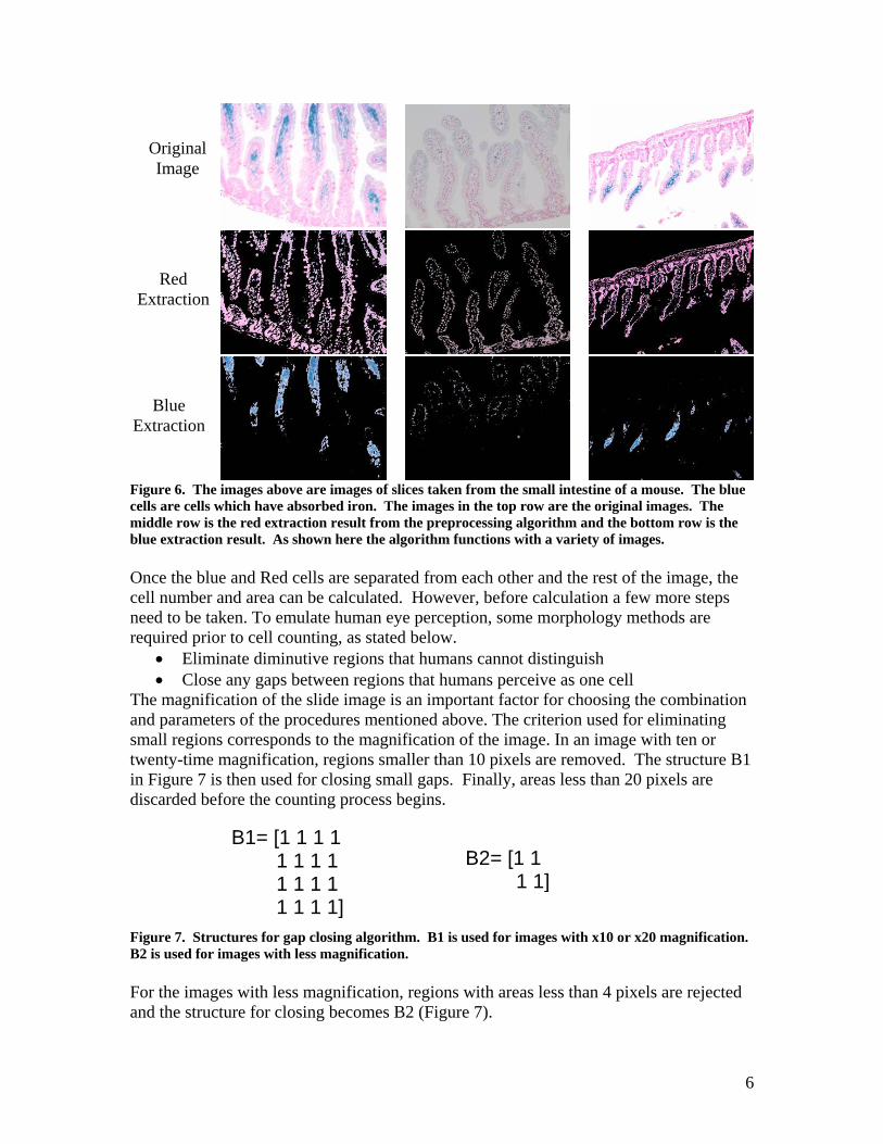
Figure 6. The images above are images of slices taken from the small intestine of a mouse. The blue cells are cells which have absorbed iron. The images in the top row are the original images. The middle row is the red extraction result from the preprocessing algorithm and the bottom row is the blue extraction result. As shown here the algorithm functions with a variety of images. Once the blue and Red cells are separated from each other and the rest of the image, the cell number and area can be calculated. However, before calculation a few more steps need to be taken. To emulate human eye perception, some morphology methods are required prior to cell counting, as stated below.

• Eliminate diminutive regions that humans cannot distinguish • Close any gaps between regions that humans perceive as one cell

The magnification of the slide image is an important factor for choosing the combination and parameters of the procedures mentioned above. The criterion used for eliminating small regions corresponds to the magnification of the image. In an image with ten or twenty-time magnification, regions smaller than 10 pixels are removed. The structure B1 in Figure 7 is then used for closing small gaps. Finally, areas less than 20 pixels are discarded before the counting process begins.

Figure 7. Structures for gap closing algorithm. B1 is used for images with x10 or x20 magnification. B2 is used for images with less magnification. For the images with less magnification, regions with areas less than 4 pixels are rejected and the structure for closing becomes B2 (Figure 7).

Original Image

Red Extraction

Blue Extraction

B1= [1 1 1 1 1 1 1 1 1 1 1 1 1 1 1 1]

B2= [1 1 1 1]

7

The counting algorithm is simple but time consuming and computation heavy. First, the connected region in the image will be detected by using dilation on any pixels with the value of ‘1’ until the output of dilation converges. Then, the region will be subtracted from the image being counted and the number of cells is increased by one. The operation is repeated until all the pixels are ‘0’in the image. (Appendix B)

Ori

gin

al im

age

(1x)

1x Algorithm 10x Algorithm

Blu

e ar

ea

76 cells; 3,455 pixels

45 cells, 5122 pixels

Red

are

a

49 cells; 4,439 pixels

17 cells, 4,011 pixels

Figure 8. Final result of applying unsuitable algorithm to the image compared to the proposed algorithm. If the user chooses the incorrect magnification of the image, undesirable results may occur. Using an unsuitable algorithm will generate incorrect results especially when implementing the algorithm for ten times magnification on less magnified image. This is because a number of cells would be merged or deleted. (Figure 8). A summarization of the algorithm is displayed in Figure 9.

8

Background Extraction

Binary image

Stretching Transformation

Blue pixels Red pixels

Original Image

Blue Extraction

Red Extraction

Calculate: Cell number Area Percentage

Dilation/Erosion

intersect

intersect

dilate

Background Extraction

Binary image

Stretching Transformation

Blue pixels Red pixels

Original Image

Blue Extraction

Red Extraction

Calculate: Cell number Area Percentage

Dilation/Erosion

intersect

intersect

dilate

Figure 9. A graphical flow chart for the final algorithm. Graphical User Interface Since this algorithm would be used by researchers who do not have a strong programming background, a graphical user interface was created for ease of use. The interface allows the user to choose a certain part of the image, if an analysis of the whole image is not needed (Figure 10). It also allows the user to choose the magnification of the image so the correct structures are used in the processing algorithm (Figure 10). A final output is given to the user which contains values such as the red and blue area, the number of blue and red cells, and the percentage of blue and red cells for the selected region (Figure 11).

Figure 10. The user is first asked for the image magnification (top left box) so that the correct masks are used in the algorithm. The user can then select an area of the image (image on the right) or choose to analyze the entire image (bottom left box).

9

Figure 11. After a selection is made the algorithm will separate the blue and red pixels from the selected area (left) and give an output of number of cells, area, and percentages (right). Results The algorithm was tested on a variety of images and the resulting cell count is similar to a manual count of the blue cells. The red cell count can be inaccurate at times when the cells are located close to one another. When the cells are connected the algorithm may count a group of cells as one cell. This is only a minor detail since red cells are not of great importance, and is also why the area and percentage are calculated. In all the images where blue cells could be distinguished visually the number was roughly equal to the manual count. Below are some of the test results.

Comparison of Algorithm and Manual Blue cell Analysis Image Manual Algorithm Results

1 29 cells 30 cells 2 23 cells 22 cells 3 ~70-65% 60.5% 4 28 cells 21 cells

10

Selected image Extraction of Blue Extraction of Red

Selected image Extraction of Blue Extraction of Red

Selected image Extraction of Blue Extraction of Red

Selected image Extraction of Blue Extraction of Red

Figure 12. In the table above results from the counting test are listed. Selections of the image were manually counted and then the algorithm was run. The corresponding images are above. If blue cells could not be distinguished a percentage of blue cells were used (image 3). All the images are 10x or 20x except image 4 which used the less magnification algorithm. The manual counting was done by an inexperienced individual. As shown above the manual count or approximation is similar to that of the algorithm. Image 4 in Figure 12 was one of less magnification. This makes it difficult to distinguish what is a single blue cell, visually and computationally. Due to less magnification there was a larger scale of error; however, the manual count and algorithm results were still fairly close to one another. Discussion Overall the algorithm works well for the purposes of the Kling Lab. Due to some error in counting of images with less magnification, the lab may choose only to use images of x10 or x20 magnification. The program seems to count the number/area of blue cells correctly for all the images we were provided; however, further testing may be required before the algorithm can be used in practice. Compared to the previous method of manual counting, this algorithm is a vast improvement. It requires little user input and takes only a few seconds to count the cells

Image 1 Image 2

Image 3 Image 4

11

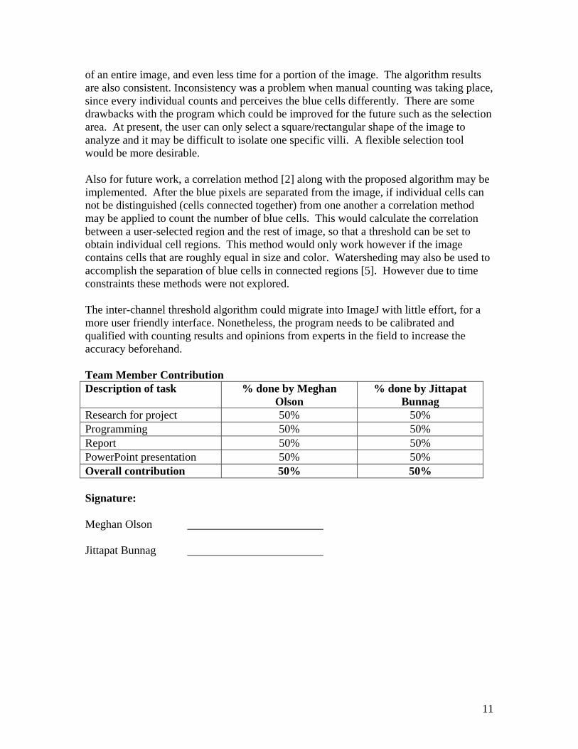
of an entire image, and even less time for a portion of the image. The algorithm results are also consistent. Inconsistency was a problem when manual counting was taking place, since every individual counts and perceives the blue cells differently. There are some drawbacks with the program which could be improved for the future such as the selection area. At present, the user can only select a square/rectangular shape of the image to analyze and it may be difficult to isolate one specific villi. A flexible selection tool would be more desirable. Also for future work, a correlation method [2] along with the proposed algorithm may be implemented. After the blue pixels are separated from the image, if individual cells can not be distinguished (cells connected together) from one another a correlation method may be applied to count the number of blue cells. This would calculate the correlation between a user-selected region and the rest of image, so that a threshold can be set to obtain individual cell regions. This method would only work however if the image contains cells that are roughly equal in size and color. Watersheding may also be used to accomplish the separation of blue cells in connected regions [5]. However due to time constraints these methods were not explored. The inter-channel threshold algorithm could migrate into ImageJ with little effort, for a more user friendly interface. Nonetheless, the program needs to be calibrated and qualified with counting results and opinions from experts in the field to increase the accuracy beforehand. Team Member Contribution Description of task % done by Meghan

Olson % done by Jittapat

Bunnag Research for project 50% 50% Programming 50% 50% Report 50% 50% PowerPoint presentation 50% 50% Overall contribution 50% 50% Signature: Meghan Olson Jittapat Bunnag

12

References [1] Kleven, Kelsey. Analyzing for the Presence of Iron in Small Intestinal Villi [Online].

http://homepages.cae.wisc.edu/~ece533/project/villicount/kleven030429.html [April 29, 2003].

[2] Wang, Yang and Pei Qi. Small Intestine Villi Counting [Online]. http://homepages.cae.wisc.edu/~ece533/project/f05/wang_qi.txt [December 2005].

[3] Nemours Foundation. Anemia. Available [Online] http://kidshealth.org/parent/medical/heart/anemia.html. Retrieved December 2005.

[4] All about Anemia. Available [Online] http://www.anemia.com/overview/overview.html. Retrieved December 2005.

[5] Malpica, Norberto et. al. Applying Watershed Algorithms to the Segmentation of Clustered Nuclei. Cytometry, 28: 289-297. 1997.

13

Appendix A : Proposed Algorithm Code function Count_cells(file) % Count number of Red Blood Cell absorbing iron % Uasge Count_cells(IMG File) % % Program for ECE 533 Fall 2005 project % (C) 2005 by Jittapat Bunnag & Meghan Lynn Olson % % Description: Allows user to open and view an image file of a villi slide. % The user can then select what magnification the image was taken. % The user also selects either an area of the image that is of interest to % them or the entire image. The program will then seperate the red and blue % cells in the image. The number of blue cells are counted and the area of % the blue and red cells are calculated. % The number of blue cells, the area of blue and red cells, % and the percentatge of blue and red cells are displayed to the user. % % Created: 1 Nov 2005 % Last revised: 19 Dec 2005 (19:00) %__________________________________________________________________________ %Read in original file J=imread(file); %Strech out image so that all color levels are used (0-255) M = imadjust(J,stretchlim(J),[]); figure(1);imagesc(J); title('Original Image'); %name Original image and get size of matrix Org_Img = J; [x y]=size(Org_Img); %Green channel can select Blue and Red components %set threshold for streched image extraction G_thres1 = 140; %define filters to use with images %use for x10 or x20 image G= [0 1 0 1 1 1 0 1 0]; %use for an image with less magnification K = [0 1 1 0]; %use for x10 or x20 image H= [0 1 0 1 1 1 1 1 1 0 1 0]; %use for an image with less magnification

14

L = [0 1 1 0 0 1 1 0]; %get user input for what magnification the image is User_input= questdlg('What magnification is the image?', 'Magnification', ... 'x1','x10 or x20', 'x10 or x20'); Area_select= questdlg('Please select the area where you want to count cells.',... 'Select Villi', 'Select Area', 'Entire Image','Select Area'); switch Area_select case 'Select Area' %allow the user to choose section of image for analysis rect=getrect(figure(1)); x_min=floor(rect(1)); y_min=floor(rect(2)); width=floor(rect(3)); height=floor(rect(4)); img_sect=zeros(height,width,3); img_sect= Org_Img(y_min:(y_min+height),x_min:(x_min+width),:); %Strech out image so that all color levels are used (0-255) M = imadjust(img_sect,stretchlim(img_sect),[]); %name streched image Org_Img_Mod = M; case 'Entire Image' img_sect = Org_Img; Org_Img_Mod = imadjust(img_sect,stretchlim(img_sect),[]); end %isolate Red, Blue, and Green Channels %Modified image channels Org_Im_R = Org_Img_Mod(:,:,1); Org_Im_G = Org_Img_Mod(:,:,2); Org_Im_B = Org_Img_Mod(:,:,3); %Original image channels Org_Im_R2 = img_sect(:,:,1); Org_Im_G2 = img_sect(:,:,2); Org_Im_B2 = img_sect(:,:,3); %find size of selected part of image [m,n] = size(Org_Im_R2); %Set Temp files for the extracted and binary images Tmp_1 = img_sect; Tmp_2 = img_sect; Tmp_5 = img_sect; Tmp_9 = img_sect; Tmp_11 = img_sect; Tmp_14 = img_sect; Tmp_15 = img_sect; %binary images Tmp_3 = ones(m ,n);

15

Tmp_4 = ones(m ,n); Tmp_6 = ones(m ,n); Tmp_7 = ones(m ,n); Tmp_17 = ones(m ,n); h=waitbar(0,'Please wait while cells are counted.'); %Use same algorithm for x20 and x10 switch User_input case 'x10 or x20' %extract images from the Red, Green, and Blue channels for i = 1:m for j = 1:n %Green channel isolates Blue and Red from other parts of image %is a better isolation of red than blue from background if (Org_Im_G(i,j) >= G_thres1) Tmp_5(i,j,:) = 0; Tmp_6(i,j) = 0; end %find places where red value is greater than blue and green %(blue part of image) if Org_Im_R2(i,j)>Org_Im_G2(i,j) | Org_Im_R2(i,j)>Org_Im_B2(i,j) Tmp_7(i,j)= 0; end %extract white background if Org_Im_B2(i,j)<(Org_Im_G2(i,j)+20) & Org_Im_B2(i,j)>(Org_Im_G2(i,j)-5)... & Org_Im_R2(i,j)<(Org_Im_G2(i,j)+12) & Org_Im_R2(i,j)>(Org_Im_G2(i,j)-7) Tmp_17(i,j)= 0; end end waitbar(i/m) end %dilate background extraction use G for 20x and 10x Tmp_17= imdilate(~Tmp_17, G); %Extract Blue from Green channel and temp7 and Red channel and background B = uint8(and(Tmp_6, Tmp_7)); %extract blue from green channel and temp 7 B = uint8(and(B, ~Tmp_17)); %background extraction B = imdilate(B, G);%get back some blue that is lost B = imopen(B, H); %get rid of small noise Tmp_10(:,:,1) = Tmp_11(:,:,1) .* B; Tmp_10(:,:,2) = Tmp_11(:,:,2) .* B; Tmp_10(:,:,3) = Tmp_11(:,:,3) .* B; % Count number of Blue in this stage Tmp_B = logical(B); % [L num1] = bwlabel(Tmp_B,8); Tmp_B = bwareaopen(Tmp_B,10,4); % [L num1] = bwlabel(Tmp_B,8); Tmp_B = imclose(Tmp_B,ones(4)); % [L num1] = bwlabel(Tmp_B,8); Tmp_B1 = bwareaopen(Tmp_B,20,4); [L num1] = bwlabel(Tmp_B,8);

16

%Extract Red from the Green channel and temp7 (extraction of blue) A = uint8(and(Tmp_6,~B));%use green channel separation and the opposite %blue extration to isolate red A = uint8(and(A,~Tmp_17)); %Get rid of Background noise A = imopen(A, H);% get rid of any extra noise Tmp_8(:,:,1) = Tmp_9(:,:,1) .* A; Tmp_8(:,:,2) = Tmp_9(:,:,2) .* A; Tmp_8(:,:,3) = Tmp_9(:,:,3) .* A; % Count number of Red in this stage Tmp_A = logical(A); % [L num2] = bwlabel(Tmp_A,8); Tmp_A = bwareaopen(Tmp_A,10,4); % [L num2] = bwlabel(Tmp_A,8); Tmp_A = imclose(Tmp_A,ones(4)); % [L num2] = bwlabel(Tmp_A,8); Tmp_A = bwareaopen(Tmp_A,20,4); [L num2] = bwlabel(Tmp_A,8); %Display images to user figure(2);subplot(1,3,1);imshow(img_sect);title('Selected image'); subplot(1,3,2);imshow(Tmp_10); title('Extraction of Blue'); subplot(1,3,3);imshow(Tmp_8); title('Extraction of Red'); %display area that is used for counting figure(3);subplot(1,3,1);imshow(img_sect);title('Selected image'); subplot(1,3,2);imshow(Tmp_B); title('Blue area for counting'); subplot(1,3,3);imshow(Tmp_A); title('Red area for counting'); %calculate percentage of blue and red cells blue_area=(sum(sum(Tmp_B1))); red_area=(sum(sum(Tmp_A))); perc_blue = (blue_area/(blue_area+red_area))*100; perc_red = (red_area/(blue_area+red_area))*100; %close waitbar close(h); %display result to user x = [' Area of blue cells (pixels) : ' int2str(blue_area) ]; y = [' Number of blue cells : ' int2str(num1) ]; t = [' Area of red cells (pixels) : ' int2str(red_area) ]; g = [' Number of red cells : ' int2str(num2) ]; b = [' Percentage of blue cells : ' num2str(perc_blue, 5) ]; r = [' Percentage of red cells : ' num2str(perc_red, 5) ]; s = [' ']; result=strvcat(y,s,x,s,g,s,t,s,b,s,r); msgbox(result, 'Cell Count'); %calculate for less magnification case 'x1' %extract images from the Red, Green, and Blue channels

17

for i = 1:m for j = 1:n %Green channel isolates Blue and Red from other parts of image %is a better isolation of red than blue from background if (Org_Im_G(i,j) >= G_thres1) Tmp_5(i,j,:) = 0; Tmp_6(i,j) = 0; end %find places where red value is greater than blue and green %(blue part of image) if Org_Im_R2(i,j)>Org_Im_G2(i,j) | Org_Im_R2(i,j)>Org_Im_B2(i,j) Tmp_7(i,j)= 0; end %extract white background if Org_Im_B2(i,j)<(Org_Im_G2(i,j)+20) & Org_Im_B2(i,j)>(Org_Im_G2(i,j)-5)... & Org_Im_R2(i,j)<(Org_Im_G2(i,j)+12) & Org_Im_R2(i,j)>(Org_Im_G2(i,j)-7) Tmp_17(i,j)= 0; end end waitbar(i/m) end %dilate background extraction use K for x0 Tmp_17= imdilate(~Tmp_17, K); %Extract Blue from Green channel and temp7 and Red channel and background B = uint8(and(Tmp_6, Tmp_7)); %extract blue from green channel and temp 7 B = uint8(and(B, ~Tmp_17)); %background extraction B = imopen(B, L); %get rid of small noise Tmp_10(:,:,1) = Tmp_11(:,:,1) .* B; Tmp_10(:,:,2) = Tmp_11(:,:,2) .* B; Tmp_10(:,:,3) = Tmp_11(:,:,3) .* B; % Count number of Blue in this stage Tmp_B = logical(B); % [L num1] = bwlabel(Tmp_B,8); Tmp_B = bwareaopen(Tmp_B,4,4); % [L num1] = bwlabel(Tmp_B,8); Tmp_B = imclose(Tmp_B,ones(2)); [L num1] = bwlabel(Tmp_B,8); %Extract Red from the Green channel and temp7 (extraction of blue) A = uint8(and(Tmp_6,~B)); %extract red from green and opposite of %blue extraction A = uint8(and(A,~Tmp_17)); %get rid of Background noise A = imopen(A, G); %get rid of extra noise Tmp_8(:,:,1) = Tmp_9(:,:,1) .* A; Tmp_8(:,:,2) = Tmp_9(:,:,2) .* A; Tmp_8(:,:,3) = Tmp_9(:,:,3) .* A; % Count number of Red in this stage Tmp_A = logical(A); % [L num2] = bwlabel(Tmp_A,8);

18

Tmp_A = bwareaopen(Tmp_A,4,4); % [L num2] = bwlabel(Tmp_A,8); Tmp_A = imclose(Tmp_A,ones(2)); [L num2] = bwlabel(Tmp_A,8); %display images to user figure(2);subplot(1,3,1);imshow(img_sect);title('Selected image'); subplot(1,3,2);imshow(Tmp_10); title('Extraction of Blue'); subplot(1,3,3);imshow(Tmp_8); title('Extraction of Red'); %display area that is used for counting figure(3);subplot(1,3,1);imshow(img_sect);title('Selected image'); subplot(1,3,2);imshow(Tmp_B); title('Blue area for counting'); subplot(1,3,3);imshow(Tmp_A); title('Red area for counting'); %calculate percentage of blue and red cells %after counting process. blue_area=(sum(sum(Tmp_B))); red_area=(sum(sum(Tmp_A))); perc_blue = (blue_area/(blue_area+red_area))*100; perc_red = (red_area/(blue_area+red_area))*100; %close waitbar close(h); %display result to user x = [' Area of blue cells (pixels) : ' int2str(blue_area) ]; y = [' Number of blue cells : ' int2str(num1) ]; t = [' Area of red cells (pixels) : ' int2str(red_area) ]; g = [' Number of red cells : ' int2str(num2) ]; b = [' Percentage of blue cells : ' num2str(perc_blue,5) ]; r = [' Percentage of red cells : ' num2str(perc_red,5) ]; s = [' ']; result=strvcat(y,s,x,s,g,s,t,s,b,s,r); msgbox(result, 'Cell Count'); end

19

Appendix B: Counting algorithm of connected regions function count_region(IMG) % Count connected region in IMG % assume the background is zero % and the cell area is one % The MATLAB built-in function, bwlabel, yield the same result % with faster speed, therefore, bwlabel is implemented in final project. bw = logical(IMG); % Structure to define connected region % Use 8-connect B = logical( [1 1 1 ; 1 1 1 ; 1 1 1 ]); cell_count = 0; [m, n] = size(bw); for i = 1:m for j = 1:n if bw(i,j) x = logical(zeros(m,n)); x(i,j) = 1; converged = 0; while converged==0 xnew=logical(and(imdilate(x,B),bw)); if sum(sum(xnew-x))==0 converged = 1; end x = xnew; end bw = and(bw, not(x)); cell_count = cell_count + 1; end end end disp(['Number of cells ' int2str(cell_count)]);