Short-lived brominated hydrocarbons – observations in the ... · were opened and ﬂushed with ambient air for about 20s. Us-ing a reciprocating pump, ... research vessel “Sonne”

Atmos. Chem. Phys., 12, 1213–1228, 2012www.atmos-chem-phys.net/12/1213/2012/doi:10.5194/acp-12-1213-2012© Author(s) 2012. CC Attribution 3.0 License.

AtmosphericChemistry

and Physics

Short-lived brominated hydrocarbons – observations in the sourceregions and the tropical tropopause layer

S. Brinckmann1, A. Engel1, H. Bonisch1, B. Quack2, and E. Atlas3

1Institute for Atmospheric and Environmental Sciences, Universitat Frankfurt/Main, Germany2Leibniz-Institut fur Meereswissenschaften, Universitat Kiel, Germany3Rosenstiel School of Marine and Atmospheric Science, University of Miami, USA

Correspondence to:S. Brinckmann ([email protected])

Received: 7 June 2011 – Published in Atmos. Chem. Phys. Discuss.: 5 August 2011Revised: 12 December 2011 – Accepted: 9 January 2012 – Published: 1 February 2012

Abstract. We conducted measurements of the five impor-tant short-lived organic bromine species in the marine bound-ary layer (MBL). Measurements were made in the NorthernHemisphere mid-latitudes (Sylt Island, North Sea) in June2009 and in the tropical Western Pacific during the Trans-Brom ship campaign in October 2009. For the one-weektime series on Sylt Island, mean mixing ratios of CHBr3,CH2Br2, CHBr2Cl and CH2BrCl were 2.0, 1.1, 0.2, 0.1 ppt,respectively. We found maxima of 5.8 and 1.6 ppt for thetwo main components CHBr3 and CH2Br2. Along the cruisetrack in the Western Pacific (between 41◦ N and 13◦ S) wemeasured mean mixing ratios of 0.9, 0.9, 0.2, 0.1 and 0.1 pptfor CHBr3, CH2Br2, CHBrCl2, CHBr2Cl and CH2BrCl. Airsamples with coastal influence showed considerably highermixing ratios than the samples with open ocean origin. Cor-relation analyses of the two data sets yielded strong lin-ear relationships between the mixing ratios of four of thefive species (except for CH2BrCl). Using a combined dataset from the two campaigns and a comparison with the re-sults from two former studies, rough estimates of the mo-lar emission ratios between the correlated substances were:9/1/0.35/0.35 for CHBr3/CH2Br2/CHBrCl2/CHBr2Cl. Ad-ditional measurements were made in the tropical tropopauselayer (TTL) above Teresina (Brazil, 5◦ S) in June 2008, usingballoon-borne cryogenic whole air sampling technique. Nearthe level of zero clear-sky net radiative heating (LZRH) at14.8 km about 2.25 ppt organic bromine was bound to the fiveshort-lived species, making up 13 % of total organic bromine(17.82 ppt). CH2Br2 (1.45 ppt) and CHBr3 (0.56 ppt) ac-counted for 90 % of the budget of short-lived compoundsin that region. Near the tropopause (at 17.5 km) organic

bromine from these substances was reduced to 1.35 ppt, with1.07 and 0.12 ppt attributed to CH2Br2 and CHBr3, respec-tively.

1 Introduction

Reactive halogens, especially chlorine and bromine com-pounds, contribute to the decomposition of stratosphericozone. In addition to mainly anthropogenic long-lived sourcegases like chlorofluorocarbons (CFC), chlorocarbons, or bro-mofluorocarbons (Halon fire suppressants), other substanceswith atmospheric lifetimes shorter than six months, often re-ferred to as very short-lived substances (VSLS), have thepotential to transport a significant amount of reactive halo-gen into the stratosphere. A significant impact to the strato-spheric bromine budget is expected from brominated VSLSspecies, whose sources are predominantly natural. Bro-moform (CHBr3), dibromomethane (CH2Br2) and the threepolyhalogenated species CHBr2Cl, CHBrCl2 and CH2BrClhave been identified as the most important short-lived car-riers of atmospheric bromine. Highest concentrations ofbrominated VSLS are usually found in coastal regions,which is commonly attributed to emissions from macroal-gae (Montzka et al., 2011). Typically lower values havebeen measured above the open ocean (e.g. Quack and Wal-lace, 2004), except for certain upwelling regions (e.g. Classand Ballschmiter, 1988; Quack et al., 2004; Carpenter etal., 2007), where a high abundance of phytoplankton is ex-pected to account for strong emissions of these bromocar-bons. Several studies (e.g. Yokouchi et al., 2005; O’Brien

Published by Copernicus Publications on behalf of the European Geosciences Union.

1214 S. Brinckmann et al.: Short-lived brominated hydrocarbons

et al., 2009) have found good correlations for at least threeof the brominated VSLS (CHBr3, CH2Br2 and CHBr2Cl),which suggests common sources and consistent emission ra-tios between these compounds.

There is a large uncertainty about the amount of brominetransported into the stratosphere by brominated VSLS. Veryfew measurements of these species in the entrance region tothe stratosphere have been published to date (e.g. Schauffleret al., 1999; Laube et al., 2008; Liang et al., 2010). Based onorganic bromine source gas data in the tropical tropopauselayer (TTL) and the results from modeling studies concern-ing the transport of these gases and their degradation prod-ucts into the stratosphere, Montzka et al. (2011) have deter-mined that brominated VSLS contribute between 1 and 8 pptto stratospheric inorganic bromine (Bry). Stratospheric mea-surements of BrO (one of the main products resulting fromthe degradation of the VSLS) have indicated values of about3–7 ppt Bry that could be attributed to this additional inputfrom VSLS (Dorf et al., 2006). Because of large variabil-ity in source emissions and uncertainty in quantifying trans-port pathways to the upper tropical troposphere, determina-tion of the global transport of reactive halogens through theTTL and into the stratosphere is a difficult issue. Severalstudies emphasise the importance of certain regions, in par-ticular the Western Pacific region, on the transport of VSLSfrom the source areas to the TTL (Gettelman et al., 2002;Fueglistaler et al., 2004; Aschmann et al., 2009). These ob-servations underline the necessity and importance of VSLSmeasurements in the marine boundary layer (MBL) and inthe TTL of these specific regions to improve the quantitativeunderstanding of the troposphere-to-stratosphere transport ofbromine from VSLS.

2 Measurements

2.1 Sampling and analysis

Two-litre electropolished stainless steel canisters of the sametype were used for both the Sylt Island and TransBrom sam-ple collection. The one-week air sampling campaign in Liston the island of Sylt (North Sea, 55.02◦ N, 8.43◦ E, 2 m a.s.l.)was performed in June 2009. 46 air samples were collectedbetween 22 June 18:00 UTC and 29 June 09:00 UTC, with atime resolution of three hours (except for a break between21:00 and 03:00 at night). The sampling was carried outabout 100 m from the eastern coast of Sylt Island. This east-ern coastline is characterized by tidal flats, while the westerncoast is oriented to the open sea. The evacuated canisterswere opened and flushed with ambient air for about 20 s. Us-ing a reciprocating pump, the canisters were then filled toa pressure of approximately 2.5 bar. About one week afterthe measurement campaign the air samples were analysed atthe Institut fur Atmosphare und Umwelt (IAU) Frankfurt us-ing an Agilent-7890 gas chromatography system with mass

Table 8. Comparison of estimated SGI and PGI (in ppt Br) for the five brominated VSLS, in a simple approach

derived from the two TTL samples B44-15 and B44-12 (see table 6).

Compound SGI+PGI SGI SGI Relative

CH2Br2 1.452 1.074 74%

CHBr3 0.564 0.120 21%

CHBrCl2 0.083 0.055 66%

CH2BrCl 0.082 0.067 82%

CHBr2Cl 0.072 0.034 47%

Total VSLS 2.253 1.350 60%

Fig. 1. Cruise track of research ship “Sonne” during “TransBrom” measurement campaign in October 2009.

The red dots mark the location of the 23 air samplings for the IAU Frankfurt data set.

Fig. 2. Chromatogram in NCI mode on Br ion mass 79 during TransBrom measurements.

23

Fig. 1. Cruise track of research ship “Sonne” during “TransBrom”measurement campaign in October 2009. The red dots mark thelocation of the 23 air samplings for the IAU Frankfurt dataset.

spectrometric detection (GC-MSD) in electron impact ioni-sation (EI) mode. We obtained mixing ratio time series forfour of the brominated VSLS: CH2Br2, CHBr3, CHBr2Cland CH2BrCl.

During the TransBrom measurement campaign aboard theresearch vessel “Sonne” in the West Pacific in October 2009(see overview paper by Kruger and Quack, 2012) we col-lected 23 air samples between 41◦ N and 13◦ S latitude. Thetrack of the ship and the coordinates of the sampling loca-tions are illustrated in Fig.1. The sampling started nearthe northern coast of the Japanese main island Honshu andended about 300 km southeast of the coast of Papua NewGuinea. Using a metal bellows pump, the sample canisterswere flushed five times before being filled to the final sam-ple pressure of 2 bar. The air samples were collected twotimes per day, at around 11:00 and 23:00 UTC (21:00 and09:00 LT), during the last three days only one sampling perday (at 23:00 UTC) was carried out. The measurements wereconducted on 14 January 2010 at the IAU using the afore-mentioned GC-MSD system in negative ion chemical ionisa-tion (NCI) mode. With this detection mode we could achievea very precise analysis at very low detection limits of all fivebrominated VSLS. Figure2 shows a NCI chromtogram forbromine ion mass 79 as obtained during the TransBrom mea-surements.

During the same campaign in the Western Pacific an ad-ditional set of air samples was collected using 2.3-litre elec-tropolished stainless steel canisters. The sampling procedurewas the same as described above for the TransBrom IAU dataset. The measurements were conducted at the University of

Atmos. Chem. Phys., 12, 1213–1228, 2012 www.atmos-chem-phys.net/12/1213/2012/

S. Brinckmann et al.: Short-lived brominated hydrocarbons 1215

Table 8. Comparison of estimated SGI and PGI (in ppt Br) for the five brominated VSLS, in a simple approach

derived from the two TTL samples B44-15 and B44-12 (see table 6).


CH2Br2 1.452 1.074 74%

CHBr3 0.564 0.120 21%

CHBrCl2 0.083 0.055 66%

CH2BrCl 0.082 0.067 82%

CHBr2Cl 0.072 0.034 47%

Total VSLS 2.253 1.350 60%

Fig. 1. Cruise track of research ship “Sonne” during “TransBrom” measurement campaign in October 2009.

The red dots mark the location of the 23 air samplings for the IAU Frankfurt data set.


23


Miami using a HP 5971 GC/MSD system in EI mode (seeSchauffler et al., 1999 for a detailed description). A data setof 73 samples with mixing ratios for three of the five bromi-nated VSLS (CH2Br2, CHBr2Cl, CHBr3) covering the wholetrack between Japan and Australia was obtained. This dataset also will be used in the analysis of typical emission ratios(Sect.4.2). A detailed presentation of these time series anal-ysed at Miami focusing on a source analysis will be given ina study by K. Kruger (personal communication, 2011).

In May and early June 2008 our group participated in aballoon campaign in Teresina (Brazil), located in the tropicsat 5.07◦ S, 42.87◦ W. The balloon carrying the whole air sam-pler BONBON-I (see Schmidt et al., 1987) was launched on1 June 2008 by the French Space Agency CNES (Centre Na-tional d’ Etudes Spatiales). We collected two samples in theTTL, at altitudes of 14.8 and 17.5 km. The laboratory anal-yses were conducted in July and August of the same yearon the Agilent-7890 GC-MSD and another GC-MSD system(Sichromat 1) using both detector modes EI and NCI for eachsystem. We obtained mixing ratios for the complete spectrumof brominated species, the long-lived and the VSLS.

2.2 Sample stability

For the canisters used during List and TransBrom we testedpossible concentration drifts of bromocarbons after long pe-riods of storage. These tests indicated stronger exponentialdeclines of the mixing ratios for some of the VSLS, espe-cially CHBr3, when dry air samples were stored. In case ofsamples with typical tropospheric H2O mixing ratios a goodstability for all measured compounds was observed over thefive month test period.

The storage of dry stratospheric air samples in the canis-ters of the whole air sampler BONBON-I is also indicated tobe problematic for some of the shorter-lived bromocarbons.A repeated measurement of the two TTL samples (using EI

mode only) one year after the initial analysis revealed con-centration decreases for CH3Br, CH2Br2 and CHBr3, withhighest reductions (to about 30 % relative to the initial mea-surement) for CHBr3. For the temporal stability of CHBr2Cland CHBrCl2 no conclusions could be drawn from this ex-periment, as the unfavourable EI mode did not allow a peakdetection of these species. So, the results of the repeatedmeasurement of the two stratospheric air samples imply thatthe outcomes from the initial analysis could underestimatethe real mixing ratios at the sampling. This issue will be dis-cussed in Sect.5.1.

2.3 Scale uncertainties

For the bromine budget presented in Sect.5.1we determinedtotal uncertainties of the analysed mixing ratios. This calcu-lation was done similar to the procedure described by Laubeet al. (2008). Statistical errors during the measurementsand the systematic error of the calibration scale of the pri-mary standard gas are considered. For the two statistical er-rors we used the 1σ measurement precision of the compara-tive measurements, for the calibration scale uncertainties thecorresponding values specified by the NOAA were applied,which are 3.3 % for halon-1301, 0.2 % for halon-1211, 1.1 %for CH3Br, 6.3 % for CH2Br2 and 8.3 % for CHBr3. Forhalon-1202, halon-2402, CH2BrCl, CHBrCl2 and CHBr2Clwe used a calibration based on comparative measurementsof our primary standard gas with a calibration standard at theuniversity of East Anglia (UEA), for which we assumed rel-atively high systematic errors of 5 % for halon-2402, 10 %for halon-1202 and 20 % for the three polyhalogenated com-pounds in the overall uncertainty calculations. Possible tem-poral drifts of the substances in the canisters, as indicated bythe experiment described in Sect.2.2, were not considered inthese calculations. An estimate of this potential error is givenin Sect.5.1.

www.atmos-chem-phys.net/12/1213/2012/ Atmos. Chem. Phys., 12, 1213–1228, 2012


Table 1. Statistics for the 46 air samples from List, calculated forthe analysed brominated VSLS. The variability is defined here asthe 1σ standard deviation. The measurement precision specifiesthe 1σ standard deviation estimated for the average mixing ratiosof the samples.

Substance Mean Mix. Ratio Variability Precisionand Range [ppt] [ppt] [ppt]

CHBr3 2.02 (1.27–5.80) 0.882 (43 %) 0.023 (1.1 %)CH2Br2 1.07 (0.92–1.55) 0.127 (12 %) 0.020 (1.9 %)CHBr2Cl 0.16 (0.11–0.28) 0.033 (21 %) 0.011 (6.7 %)CH2BrCl 0.10 (<0.08–0.15) 0.017 (17 %) 0.020 (20 %)

3 Observations source regions

3.1 List

Table 1 shows the statistical summary of the four bromi-nated VSLS measured at Sylt Island. CHBr3 is by far themost abundant of the four gases, with an average of 2.02 ppt,while CH2Br2 exhibits a mean of 1.07 ppt. The values forthe two species lie on the lower end of the range of means re-ported for other coastal regions (compare e.g. Zhou et al.,2008; Carpenter et al., 2005). Average and variability ofCHBr3 are considerably enhanced by a high-concentrationevent with two elevated values (up to 5.8 ppt) on 25 June. Thetwo polyhalogenated show relatively low mixing ratios, espe-cially CH2BrCl with an estimated average of only 0.10 ppt.Some of the signals of the latter compound are below the de-tection limit of about 0.08 ppt. For statistical purposes, mea-surements for CH2BrCl that were below detection limit, wereassigned a value of 0.07 ppt. This mixing ratio is chosento match the lowest mixing ratios measured during Trans-Brom, and we think is reasonable considering its relativelylong lifetime of 137 days (under average tropospheric condi-tions, Montzka et al., 2011). The corresponding time seriesof the four species are shown in Fig.3. CH2Br2 (panel A,solid circles, left-hand scale) and CHBr3 (same graph, opencircles, right-hand scale) exhibit very similar variance pat-terns with mixing ratios peaking on 25 June at 03:00 and06:00 UTC. A qualitatively similar curve is also found forCHBr2Cl (B, solid circles, left-hand scale), while CH2BrCl(same graph, open circles, right-hand scale) – for which wecould not obtain results from the first eight canisters dueto technical problems – exhibits an independent variabilitystrongly affected by the low measurement precision. Theanalysis of backward air mass trajectories (shown in Fig.9)indicate that during the first two days of the time series theair masses passed over the North Sea before arriving at oursampling site (see example for 24 June, panel 1). The high-concentration event on 25 June (panel 2) marks a change inthe catchment area from the North Sea to the Baltic Sea. Forthe following time period until the end of the series the air

Fig. 3. A: Time series of CH2Br2 (solid circles, left-hand scale) and CHBr3 (open circles, right-hand scale)

between 22 and 29 June 2009 at List/Sylt. B: Corresponding results for CHBr2Cl (solid circles, left-hand scale)

and CH2BrCl (open circles, right-hand scale). The error bars give estimates of the 1σ measurement precision.

The numbers in panel A mark the dates corresponding to the trajectories as labeled in figure 9.

24

Fig. 3. (A) Time series of CH2Br2 (solid circles, left-hand scale)and CHBr3 (open circles, right-hand scale) between 22 and 29 June2009 at List/Sylt.(B) Corresponding results for CHBr2Cl (solid cir-cles, left-hand scale) and CH2BrCl (open circles, right-hand scale).The error bars give estimates of the 1σ measurement precision. Thenumbers in(A) mark the dates corresponding to the trajectories aslabeled in Fig.9.

masses had been transported over the Baltic Sea in an east-erly stream (see example for 29 June, panel 3).

The similar levels of short-lived bromocarbons observedfor air transported from both the North Sea and the Baltic Sealead to two important conclusions. First, the mean emissionfluxes of these species in the two environments apparentlydo not differ significantly. Second, we conclude that localsources of brominated VSLS are of minor importance, sincelocal wind directions changing from West (open sea) to East(tidal flats) have no noticeable impact on the observed mixingratios. This latter finding is also supported by the compari-son of local wind speeds and bromocarbon mixing ratios. Acorrelation between these measures was observed in formerstudies for regions with strong nearby sources (Zhou et al.,2008), but such correlation is not found for our data fromList. The elevated concentrations detected on 25 June sug-gest that the sampled air masses had crossed extended areas



Fig. 4. A: Mixing ratios of CH2Br2 (solid circles) and CHBr3 (open circles) as analysed for the 23 IAU

TransBrom air samples in the Western Pacific. B: Corresponding results for CHBrCl2 (solid circles), CHBr2Cl

(open circles) and CH2BrCl (grey symbols). The error bars give the 1σ measurement precision. The numbers

in panel A mark the sites corresponding to the trajectories as labeled in figure 10.

25

Fig. 4. (A) Mixing ratios of CH2Br2 (solid circles) and CHBr3(open circles) as analysed for the 23 IAU TransBrom air samples inthe Western Pacific.(B) Corresponding results for CHBrCl2 (solidcircles), CHBr2Cl (open circles) and CH2BrCl (grey symbols). Theerror bars give the 1σ measurement precision. The numbers inpanel(A) mark the sites corresponding to the trajectories as labeledin Fig. 10.

of coastal regimes in the transition zone between the NorthSea and Baltic Sea (compare panel 2 of Fig.9). This wouldbe consistent with the importance of bromocarbon emissionsin coastal environments.

3.2 TransBrom

The time series of the mixing ratios of the five importantbrominated VSLS for the TransBrom campaign in the WestPacific are illustrated in Fig.4. CH2Br2 (panel A, solid cir-cles) and CHBr3 (same panel, open circles) showed relativelylow mixing ratios above open ocean areas, around 0.8 ppt forCH2Br2 and around 0.6 ppt for CHBr3, while higher valuesof 1.0–1.2 ppt for CH2Br2 and 1.2–2.1 ppt for CHBr3 weredetected near the Japanese coast (at 41◦ N) and in the vicin-ity of the islands of Papua New Guinea (at 10 and 13◦ S).

Table 2. The same as in Table1 but for the 23 TransBrom IAU airsamples from the Western Pacific.

Substance Mean Mix. Ratio Variability Precisionand Range [ppt] [ppt] [ppt]

CHBr3 0.91 (0.44–2.16) 0.47 (51 %) 0.020 (2.2 %)CH2Br2 0.92 (0.69–1.21) 0.13 (15 %) 0.006 (0.6 %)CHBrCl2 0.20 (0.16–0.30) 0.04 (19 %) 0.002 (0.9 %)CHBr2Cl 0.14 (0.09–0.34) 0.04 (31 %) 0.002 (1.2 %)CH2BrCl 0.10 (0.07–0.13) 0.02 (16 %) 0.002 (2.2 %)

These observations are consistent with a strong influencefrom coastal sources and relatively weak emissions in openocean areas. The corresponding backward trajectories, dis-played in Fig.10, confirm a slowly decreasing coastal in-fluence at the beginning of the cruise, as the winds persis-tently transported air masses from the North (see examplein panel 1 for 32◦ N). Between 0 and 20◦ N typically east-erly to northerly winds advected air from open ocean re-gions, as shown on panel 2. For the air samples collectedbetween 6 and 13◦ S (panel 3, 6◦ S) air masses arrived fromthe Southeast after passing through a region with larger is-lands in the Solomon Sea. The observation of relatively lowconcentrations above most of the open ocean regions is inagreement with other studies (e.g. Quack and Wallace, 2004;Yokouchi et al., 2005). Considerably elevated mixing ratios,as reported by Atlas et al. (1993) for upwelling regions inthe equatorial Eastern Pacific, were not observed during thiscruise. This is consistent with an absence of such upwellingzones associated with high biogenic activity in the WesternPacific. Similar profiles, with elevated values near the coast-lines, were found for CHBrCl2 (Fig. 4, panel B, solid blackcircles) and CHBr2Cl (same panel, open circles). In agree-ment with our observations at List, CH2BrCl (same panel,grey circles) showed a mixing ratio time series that was notcorrelated to the other bromocarbon compounds.

A comparison with the air samples analysed at the Uni-versity of Miami (UM, not shown in the graphs) reveals intotal good agreement with the IAU measurements, especiallyfor CHBr3 and CHBr2Cl. A difference between the data isapparent for the CH2Br2, with around 20 % higher valuesfor the UM data set, while the patterns of variation matchvery well. In agreement with the findings from the IAUdata, the higher spatial resolution of the UM samples alsodoes not reveal any high-concentration events above the openocean. The elevated mixing ratios which were observed dur-ing the beginning and the end of the cruise, but which arenot covered by the IAU data, will be discussed in a study byK. Kruger (personal communication, 2011).

In Table2 a summary for the data sets from the IAU Frank-furt is shown. Due to the uneven distributions of sourcesand sinks along the track in the West Pacific the mixing ratiodata tend to be better described by a log-normal rather than



a normal distribution. Thus, the geometric values of meanand standard deviation were calculated for the overall sum-mary of this data set. (The differences between geometricand arithmetic means are very small, only for CHBr3 a sig-nificantly higher arithmetic mean (+13 %) was determined.)For the subset of open ocean samples discussed below, arith-metic means are given, as these have proven to be more ap-propriate for this case. CHBr3 shows an overall mean mix-ing ratio of 0.91 ppt, with a range between 0.44 and 2.16 ppt.As noted above, the higher values were detected for sampleswith coastal influence, while the open ocean mixing ratioswere considerably lower. When excluding all samples withtrajectories passing through regions with larger islands, wefind an average of only 0.62 ppt for CHBr3. Consideringthe whole data set, CH2Br2 exhibits an average of 0.92 pptand a range between 0.69 and 1.21 ppt. For the limited setof samples without coastal influence we obtain an averageof 0.83 ppt for this substance. Thus, above the open oceanCH2Br2 had somewhat higher concentrations than CHBr3,which can be explained by the combination of its relativelylonger lifetime and the absence of significant emissions. Thethree polyhalogenated compounds show average mixing ra-tios of 0.10, 0.20 and 0.14 ppt (for CH2BrCl, CHBrCl2 andCHBr2Cl, respectively). The corresponding open ocean val-ues of 0.09, 0.17 and 0.11 ppt (in the above order) are alsolower compared to those with coastal influence.

4 Regression analyses

In the following sections we present different regressionanalyses carried out to investigate possible relationships be-tween the mixing ratios of brominated VSLS. Several pre-vious studies reported linear relationships between the mix-ing ratios of CHBr3, CH2Br2 and CHBr2Cl (e.g. O’Brien etal., 2009; Yokouchi et al., 2005), indicating that these sub-stances share the same sources. Li et al. (1994) suggestedthe additional possibility that reactions of CHBr3 with sea-water chlorine could produce CHBr2Cl and thus account forthe observed correlations to this compound.

4.1 Linear regression

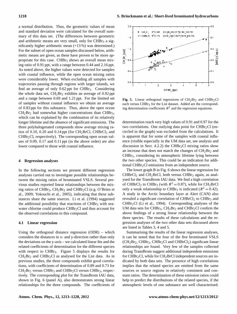
Using the orthogonal distance regression (ODR) – whichconsiders the distances in x- and y-direction rather than onlythe deviations on the y-axis – we calculated linear fits and therelated coefficients of determination for the different specieswith respect to CHBr3. Figure 5 displays the results forCH2Br2 and CHBr2Cl as analysed for the List data. As inprevious studies, the three compounds exhibit good correla-tions, with coefficients of determination of 0.89 and 0.73 forCH2Br2 versus CHBr3 and CHBr2Cl versus CHBr3, respec-tively. The corresponding plot for the TransBrom IAU data,shown in Fig.6 (panel A), also demonstrates strong linearrelationships for the three compounds. The coefficients of

Fig. 5. Linear orthogonal correlations of CH2Br2 and CHBr2Cl each versus CHBr3 for the List data set. Added

are the corresponding determination coefficients R2 and the regression equations.

26

Fig. 5. Linear orthogonal regressions of CH2Br2 and CHBr2Cleach versus CHBr3 for the List dataset. Added are the correspond-ing determination coefficientsR2 and the regression equations.

determination reach very high values of 0.91 and 0.97 for thetwo correlations. One outlying data point for CHBr2Cl (en-circled in the graph) was excluded from the calculations. Itis apparent that for some of the samples with coastal influ-ence (visible especially in the UM data set, see analysis anddiscussion in Sect. 4.2.2) the CHBr2Cl mixing ratios showan increase that does not match the changes of CH2Br2 andCHBr3, considering its atmospheric lifetime lying betweenthe two other species. This could be an indication for addi-tional CHBr2Cl emissions from an independent source.

The lower graph B in Fig.6 shows the linear regression forCHBrCl2 and CH2BrCl, both versus CHBr3 again, as anal-ysed for the TransBrom IAU data. We find a high correlationof CHBrCl2 to CHBr3 (with R2

= 0.87), while for CH2BrClonly a weak relationship to CHBr3 is indicated (R2

= 0.42).A study in the Arctic boundary layer at Alert (CAN) alsorevealed a significant correlation of CHBrCl2 to CHBr3 andCHBr2Cl (Li et al., 1994). Corresponding analyses of theUM data sets for CHBr3, CH2Br2 and CHBr2Cl confirm theabove findings of a strong linear relationship between thethree species. The results of these calculations and the re-gression analyses of the two other data sets discussed aboveare listed in Tables3, 4 and5.

Summarising the results of the linear regression analyses,it can be noted that for four of the five brominated VSLS(CH2Br2, CHBr3, CHBr2Cl and CHBrCl2) significant linearrelationships are found. Very few of the samples collectedduring TransBrom suggest additional independent emissionsfor CHBr2Cl, while for CH2BrCl independent sources are in-dicated by both data sets. The presence of high correlationsimplies that the related species are emitted from the samesources or source regions in relatively consistent and con-stant ratios. The determination of these emission ratios couldhelp to predict the distributions of the related species, if theatmospheric levels of one substance are well characterised.



Fig. 6. A: Linear orthogonal correlations of CH2Br2 (solid circles, left-hand scale) and CHBr2Cl (open circles,

right-hand scale) each versus CHBr3 for the TransBrom IAU data set (under exclusion of encircled outlying

data point). B: Corresponding analyses for CHBrCl2 (solid circles, left-hand scale) and CH2BrCl (open circles,

right-hand scale). Added are the corresponding determination coefficients R2 and the regression equations.

27

Fig. 6. (A) Linear orthogonal regressions of CH2Br2 (solid circles,left-hand scale) and CHBr2Cl (open circles) each versus CHBr3 forthe TransBrom IAU dataset (under exclusion of encircled outlyingdata point).(B) Corresponding analyses for CHBrCl2 (solid circles)and CH2BrCl (open circles). Added are the corresponding determi-nation coefficientsR2 and the regression equations.

Table 3. Linear orthogonal regression with respect to CH2Br2 andCHBr3 respectively for the List dataset, calculated for the otherbrominated VSLS, with slopem, interceptb and coefficient of de-terminationR2.

Substance Linear Regression:[Y ] =m · [X]+b

X = CH2Br2 X = CHBr3

m b R2 m b R2

CHBr3 7.3 −5.8 0.89CH2Br2 0.14 0.79 0.89CHBr2Cl 0.23 −0.09 0.75 0.03 0.10 0.73CH2BrCl 0.02 0.08 0.01 0.00 0.10 0.00

Table 4. As in Table3 but for the IAU TransBrom dataset. ForCHBr2Cl one outlying data point was excluded from the analysis.



m b R2 m b R2

CHBr3 4.0 −2.7 0.91CH2Br2 0.25 0.67 0.91CHBr2Cl 0.24 −0.09 0.91 0.07 0.07 0.97CHBrCl2 0.26 −0.03 0.73 0.07 0.13 0.87CH2BrCl 0.06 0.04 0.25 0.02 0.08 0.42

Table 5. As in Table3 but for the UM TransBrom dataset.



m b R2 m b R2

CHBr3 3.4 −2.9 0.86CH2Br2 0.29 0.84 0.86CHBr2Cl 0.36 −0.24 0.60 0.11 0.06 0.65

It should be pointed out that during the initial emission fromthe algae species into the ocean water deviating abundanceratios are expected, due to different rates of degradation inthe surface water prior to the emission through the sea sur-face. This however is not of relevance to our study as weonly consider emissions into the atmosphere and make noassumptions or conclusions about the initial emissions fromthe biological processes.

4.2 Emission ratios

4.2.1 Theoretical considerations

An intuitive approach to deriving typical emission ratiosfrom the data of compounds with similar sources is theuse of correlation plots of compound ratios versus com-pound concentration, for example, [CH2Br2]/[CHBr3] versus[CHBr3]. For this example we expect an increase of the ra-tio [CH2Br2]/[CHBr3] for decreasing CHBr3 concentrations,due to the following reasons: A stronger mixing with back-ground air always tends to enhance the [CH2Br2]/[CHBr3]ratio, as the photochemically aged background air exhibitsrelatively lower concentrations of the shorter-lived com-pound CHBr3. In addition, the stronger degradation ofCHBr3 relative to CH2Br2 (especially by photolysis) also di-rectly enhances this ratio when longer transport times occur.The smallest measured ratio in such a graph should give anestimate of the emission ratio, since these data reflect sam-ples with minimal impact from mixing and decomposition.



Three-component analyses

For a similar analysis of three well correlated compoundswith assumed constant emission ratios a plot of, for example,[CHBr3]/[CH2Br2] versus [CHBr2Cl]/[CH2Br2] can be pro-duced. Following McKeen and Liu (1993) a “dilution line”and a “chemical decay line”, both departing from the pointof the initial ratios at the time of the emission, should en-close the scattered data. The dilution line illustrates the re-lationship between the data for the case that the consideredair parcels are mixed with background air, without chemi-cal decay processes taking place. The temporal change inthe concentration of speciesX due to dilution is then deter-mined by the mixing coefficientc, its concentration[X] andits background concentration[X]b:

d[X]

dt= −c ·([X]−[X]b) (1)

Under the assumption of relatively small background con-centrations of the two shorter-lived species ([X] � [X]b and[Y ] � [Y ]b), in our case CHBr3 and CHBr2Cl, and a con-stant mixing coefficientc, the dilution or relative concentra-tion change1[X]/[X] after a given time interval1t will beequal for the two shorter-lived substances. Thus the resultingdilution line (for [X]/[Z] versus[Y ]/[Z]) has a slope of 1 ona double-logarithmic scale.

The chemical decay line describes the relationship be-tween the concentrations of the three compounds whenchanges in[X], [Y ] and [Z] are exclusively governed bychemical decomposition by a pseudo-first-order chemical re-action with the loss ratesLX, LY andLZ:d[X]

dt= −LX · [X] (2)

The loss rates are determined by the OH reaction rate coef-ficient, the OH concentration and the photolysis rate. By re-placing the loss rates of the considered compounds with thereciprocal of their local lifetimes 1/τ and solving the differ-ential equations for the concentrations of the three speciesX,Y , Z, a linear relationship can be derived for[Y ]/[Z] versus[X]/[Z] on a log-log scale representing the chemical decayline. The associated slopem is determined by the three life-times (Roberts et al., 1984; Parrish et al., 1992; McKeen andLiu, 1993):

m =1/τy −1/τz

1/τx −1/τz

(3)

McKeen and Liu (1993) have used a mesoscale model to pre-dict the concentrations of three hydrocarbons with differentlifetimes and emission rates in specific ratios. They show thatunder realistic conditions essentially all observed ratios be-tween the three species are expected to lie between the twolines, even if one of the two processes, chemical decay ordilution with background air, is excluded completely. Thisis due to processes ignored in the derivation of these lines,i.e. mixing processes with non-background air and mixing oftwo parcels characterised by different photochemical ages.

Two-component analyses

Several studies (Carpenter et al., 2003; Zhou et al., 2008) di-rectly used the linear correlation analysis between the mixingratios of e.g. CH2Br2 and CHBr3 to calculate emission ra-tios. It can be shown that under certain conditions the slopeof such a regression line is a good estimate for the initial con-centration ratio. In case of a pure dilution – an approxima-tion valid for measurements in close proximity to the sources– the initial concentration of substanceX, denoted as[X]0,decreases due to mixing with ambient air that exhibits a cer-tain background concentration[X]b as described by Eq. (1).This equation can be transformed and integrated to obtain anexponential expression for the temporal change of the con-centrations[X] and[Y ]. Assuming again a constant mixingcoefficientc (being equal for both compounds), the expo-nential term can be eliminated to obtain an equation for[Y ]

depending on[X].

[Y ] =[Y ]0−[Y ]b

[X]0−[X]b· [X]+[Y ]b−[X]b ·

[Y ]0−[Y ]b

[X]0−[X]b(4)

It can be seen that the slope of this linear relationship will beequal to the initial concentration ratio[Y ]0/[X]0 (thus to therelative emission rates) if the background concentrations ofthe two substances[X]b and[Y ]b are small compared to[X]0and[Y ]0 or if their ratios to the initial concentrations are ap-proximately equal ([X]b/[X]0 ' [Y ]b/[Y ]0), as expected forthe case of similar lifetimes. In the general case of significantbackground concentrations and differing lifetimes, as for e.g.CH2Br2 versus CHBr3, the slope of the regression line willdeviate from the initial concentration ratio.

The opposite scenario of measurements taken at a largerdistance from the regions of emission may be treated with apure chemical decay according to a pseudo first-order pro-cess, as given in Eq. (2). Similarly to the steps above, thedifferential equations can be solved for the two speciesX

andY , and the exponential time factor is eliminated to obtainthe following two equivalent expressions:

ln[Y ]

[X]=

(τx

τy

−1

)ln[X]+

(ln[Y ]0−

τx

τy

ln[X]0

)(5)

[Y ] =[Y ]0

[X]

τxτy

0

· [X]

τxτy (6)

Thus, for a plot of the natural logarithm of the ratio[Y ]/[X]

versus the natural logarithm of[X] the slope of the corre-sponding regression line is determined by the lifetimesτx

and τy . The relationship[Y ]([X]) is generally nonlinear,with a shape depending on the initial concentration ratio, theratio of the lifetimes and the concentration[X]. An analysisof Eq. (6) shows that the slope from a linear regression candeviate positively (in case of photochemically young air sam-ples) or negatively (in case of considerably aged air) fromthe real ratio of e.g. [CHBr3]0/[CH2Br2]0. If the lifetimes



Fig. 7. Linear orthogonal regressions of the natural logarithm of the ratio CH2Br2 to CHBr3 versus ln CHBr3

for the three data sets (see labels and description in the text). The corresponding determination coefficients R2

and the regression equations are listed in the graph.

Fig. 8. Ratios of [CHBr3]/[CH2Br2] versus the ratios of [CHBr2Cl]/[CH2Br2] for the the three data sets List

(blue), TransBrom IAU (black) and TransBrom UM (grey). Following an approach of McKeen and Liu (1993),

the data points are expected to be enclosed by a “dilution line” and a “chemical decay line” (whose slopes are

derived from theoretical considerations), both departing from the point with the initial abundance ratios during

the emission. The brown and green lines illustrate corresponding outcomes from Yokouchi et al. (2005) and O’

Brien et al. (2009). See text for further descriptions.

28

Fig. 7. Linear orthogonal regressions of the natural logarithm of theratio [CH2Br2] to [CHBr3] versus ln [CHBr3] for the three datasets(see labels and description in the text). The corresponding determi-nation coefficientsR2 and the regression equations are listed in thegraph.

of the two considered species are similar, Eq. (6) will re-duce to a nearly linear curve of the same form as is validfor a dilution with the constraints of zero background con-centrations. Thus, a corresponding analysis of [CHBr2Cl]versus [CH2Br2] or [CHBr3] is less sensitive (compared to[CH2Br2] versus [CHBr3]) to the photochemical age of theconsidered air masses, and the slope of the regression lineyields a relatively stable estimate of the emission ratio. Thesame conclusions can be drawn for the scenario of a pure di-lution: a mixing under consideration of realistic backgroundvalues leads to relatively smaller deviations in the slope fromthe case with zero background if the lifetime differences arealso relatively smaller.

4.2.2 Analyses and discussion

Two-component analyses

The linear regression for the List dataset yields a slope of0.14 for CH2Br2 versus CHBr3. This value is in good agree-ment with other published data from coastal mid-latitudesites, as the 0.15 determined for measurements at Mace Head(Carpenter et al., 2003) and 0.14 derived from measurementsin the seacoast region of New Hampshire (Zhou et al., 2008).The results for the TransBrom IAU data indicate a higherslope of 0.25 for the two species, which can be explainedby a stronger impact of chemical decay on the concentrationratios.

Following Carpenter et al. (2003) a correlation accordingto Eq. (5) was investigated to evaluate the impact from degra-dation processes. The results of these analyses for CH2Br2and CHBr3, the two species with a relatively large lifetime

difference, are displayed in Fig.7. The correlations for thethree datasets (List, TransBrom IAU, TransBrom UM) arevery strong, with determination coefficients between 0.97and 0.98. According to Eq. (5) the slopes correspond to life-time ratiosτCHBr3/τCH2Br2 of 0.32, 0.27 and 0.28 for List,TransBrom IAU and TransBrom UM, respectively. The life-time values published by Hossaini et al. (2010) (CHBr3: 16days, CH2Br2: 52 days, for the near-surface tropics) andMontzka et al. (2011) (CHBr3: 24 days, CH2Br2: 123 days,for average tropospheric conditions) would correspond tolifetime ratios of 0.31 and 0.20, respectively. Our findingsagree very well with these bounds, which is, in combina-tion with the strength of the correlations, a good indicationthat degradation processes had a strong impact on the anal-ysed distributions of the brominated compounds in List andabove the Western Pacific. This implies that the relation-ship between [CH2Br2] and [CHBr3] is expected to followa non-linear function according to Eq. (6) so that the slope ofthe corresponding regression line would alter with the pho-tochemical age of the considered air parcels.

Regarding the results for CHBr2Cl, we obtain very similarslopes of 0.23 and 0.24 (versus CH2Br2, see Tables3 and4)for List and TransBrom IAU. As discussed in the previoussection, the possible deviations of the slope values from theemission ratio are relatively smaller compared to the find-ings for CH2Br2 versus CHBr3, since the lifetime ratio ofCHBr2Cl to CH2Br2 is closer to 1 (about 0.6, lifetime es-timates of CHBr2Cl discussed below). Thus, the derivedslopes should yield good estimates for the correspondingemission ratios. For CHBrCl2, analysed only for the Trans-Brom data, an emission ratio of 0.26 to CH2Br2 (see Table4)can be derived from the regression analysis.

Three-component analyses

In the following section we use the approach of McKeen andLiu (1993), explained above, to derive estimates for the emis-sion ratios of CHBr3/CH2Br2/CHBr2Cl. Using Eq. (3) (withX = CHBr2Cl, Y = CHBr3, Z = CH2Br2) and applying locallifetimes of 26, 69 and 120 days for CHBr3, CHBr2Cl andCH2Br2 (Ko et al., 2003; Yokouchi et al., 2005; O’Brien etal., 2009) the slope for the chemical decay line on a double-logarithmic scale is calculated to be 4.89. As noted above,we expect a slope of 1 for a dilution line based on the as-sumption of pure dilution processes. To estimate emissionratios from a broad database containing samples of a rangeof characteristics (in terms of dilution and chemical decayprocesses), we combined the data sets from the two sourceregions under the assumption of (1) similar relative emis-sion strengths and (2) similar lifetime ratios in both regions.(1) Is supported by the above findings of the two-componentanalyses. (2) Is also justified, given that only the ratios ofthe lifetimes must be similar. Hossaini et al. (2010) foundaltitude dependent ratios of the local tropical lifetimes forCHBr3 and CH2Br2 ranging from 0.31 (16/52 days) near the



Fig. 7. Linear orthogonal regressions of the natural logarithm of the ratio CH2Br2 to CHBr3 versus ln CHBr3

for the three data sets (see labels and description in the text). The corresponding determination coefficients R2

and the regression equations are listed in the graph.

Fig. 8. Ratios of [CHBr3]/[CH2Br2] versus the ratios of [CHBr2Cl]/[CH2Br2] for the the three data sets List

(blue), TransBrom IAU (black) and TransBrom UM (grey). Following an approach of McKeen and Liu (1993),

the data points are expected to be enclosed by a “dilution line” and a “chemical decay line” (whose slopes are

derived from theoretical considerations), both departing from the point with the initial abundance ratios during

the emission. The brown and green lines illustrate corresponding outcomes from Yokouchi et al. (2005) and O’

Brien et al. (2009). See text for further descriptions.

28

Fig. 8. Ratios of [CHBr3]/[CH2Br2] versus the ratios of[CHBr2Cl]/[CH2Br2] for the the three datasets List (blue), Trans-Brom IAU (black) and TransBrom UM (grey). Following an ap-proach of McKeen and Liu (1993), the data points are expected tobe enclosed by a “dilution line” and a “chemical decay line” (whoseslopes are derived from theoretical considerations), both departingfrom the point with the initial ratios during the emission. The brownand green lines illustrate corresponding outcomes from Yokouchi etal. (2005) and O’ Brien et al. (2009). See text for further descrip-tions.

surface to 0.09 (21/237 days) in the upper troposphere (500–200 hPa region). For the lower troposphere (1000–500 hPa)Hossaini et al. (2010) report a ratio of 0.26 (17/65 days). Thiscompares rather well with the ratio of local lifetimes of 0.22(26/120 days) given by Ko et al. (2003) for average tropo-spheric conditions at about 500 hPa altitude. This shows thatthe lifetime ratios vary mainly with altitude and less withlatitude. As all our observations are in the marine bound-ary layer, we expect that they have experienced similar life-time ratios during their transport history from the sources tothe place of observation, which is the prerequisite for usingEq. (3).

The corresponding plot for the three data sets is shown inFig.8. With the constraints for the dilution line to intersect atthe upper left and the chemical decay line to intersect at thelower right portion of the data points, so that all values are en-closed by the two lines, we construct the intersection of thetwo lines based on the data sets List + TransBrom IAU (blueand black symbols) in point A, which yields the followinglower estimate for the emission ratios of the three consideredcompounds: 0.24 and 4.9 for CHBr2Cl and CHBr3, both rel-ative to CH2Br2.

Due to significant scale differences between the IAU andthe UM data we standardised the data from Miami beforeadding them to the plot by applying a linear regression forthe 23 air samples collected nearly at the same time (withtime lags of about 5 min). The correlations between the

two data sets (see Fig.11) are very strong, with determina-tion coefficients of 0.98, 0.95 and 0.92 for CHBr3, CH2Br2and CHBr2Cl, which justifies the use of this approach. TheTransBrom UM data treated in this way (displayed in grey)are generally consistent with the corresponding IAU data andthe position derived for the two lines. A relatively lowermeasurement precision, especially for the CHBr2Cl mea-surements at Miami, accounts for the larger scatter of thesedata. Nevertheless, as already indicated by the linear regres-sion analysis above, several points (identical with some ofthe coastal values discussed in Sect.4.1) clearly fall outsidethe area spanned by the two lines derived from the two otherdata sets, because of unexpectedly high CHBr2Cl mixing ra-tios. We ignore these values when determining the dilutionline, assuming that the outliers are a result of additional in-dependent sources for this compound.

Many of the West Pacific data points lie close to the chem-ical decay line, which is consistent with the observation ofvery low mixing ratios above the open ocean caused by in-tense decomposition during long transport times. The Listdata exhibit a larger variation, with at least two points (iden-tical with the mixing ratio maxima for CHBr3 and CH2Br2)suggesting a significant impact from dilution processes. Butas indicated by the findings in Fig.7 most of the List dataalso emphasize the influence of degradation processes ratherthan of a pure mixing with background air. So, a realisticposition of the dilution line is likely to be somewhat higherthan drawn, as would be the initial concentration ratios.

The findings of Yokouchi et al. (2005), drawn in the samegraph (in brown), are based on various data sets from coastaland open ocean sites in the Pacific. Very high mixing ratios,as found in this study on San Cristobal Island and ChristmasIsland, determine the position of the two bounding processlines and the resulting emission ratios (0.7; 9). The rela-tively high CHBr3/CH2Br2 ratio of 9 may reflect the closerproximity to the sources for some of the measurements. Butthe high ratio of CHBr2Cl to CH2Br2 reported by Yokouchiet al. (2005) is clearly different from our findings, as someof the List data would lie outside of the brown dashed dilu-tion line based on that study. Deviations in the calibrationscale for CHBr2Cl and/or differences in the emission ratiosbetween the different source regions could be plausible ex-planations for these differences. Measurements at the CapeVerde Islands (results added in green), evaluated with thesame method by O’Brien et al. (2009), also revealed an emis-sion ratio of 9 for CHBr3/CH2Br2, but a somewhat smallerratio of 0.46 for CHBr2Cl/CH2Br2.

The lifetime values used for the calculation of the chem-ical decay line in the above analysis are estimates based onaverage tropospheric conditions (Ko et al., 2003). These val-ues have been updated in the new WMO report to 24, 59and 123 days for CHBr3, CHBr2Cl and CH2Br2 (Montzkaet al., 2011). The updated lifetimes yield a different slopefor the chemical decay line of 3.80. Furthermore, the rel-atively high near-surface temperatures in the tropics favour



Fig. 9. Four-day backward trajectories for June 24 and 29 (left and right panel) 2009 00

UTC using HYSPLIT model and the FDAS global meteorological data set provided by the NOAA

(http://ready.arl.noaa.gov/HYSPLIT.php). The middle plot shows corresponding two-day backward trajectories

for June 25, ending at 03 (blue line) and 06 UTC (red line), the times of considerably elevated bromocarbon

levels.

Fig. 10. Five-day backward trajectories for three sampling sites along the cruise in the Western Pacific using

HYSPLIT model and the FNL global meteorological data set from NOAA.

29

Fig. 9. Four-day backward trajectories for 24 and 29 June (left and right panel) 2009 00:00 UTC using HYSPLIT model and the FDASglobal meteorological dataset provided by the NOAA (http://ready.arl.noaa.gov/HYSPLIT.php). The middle plot shows corresponding two-day backward trajectories for 25 June, ending at 03:00 (blue line) and 06:00 UTC (red line), the times of considerably elevated bromocarbonlevels.

Fig. 9. Four-day backward trajectories for June 24 and 29 (left and right panel) 2009 00

UTC using HYSPLIT model and the FDAS global meteorological data set provided by the NOAA

(http://ready.arl.noaa.gov/HYSPLIT.php). The middle plot shows corresponding two-day backward trajectories

for June 25, ending at 03 (blue line) and 06 UTC (red line), the times of considerably elevated bromocarbon

levels.

Fig. 10. Five-day backward trajectories for three sampling sites along the cruise in the Western Pacific using

HYSPLIT model and the FNL global meteorological data set from NOAA.

29

Fig. 10. Five-day backward trajectories for three sampling sites along the cruise in Western Pacific using HYSPLIT model and the FNLglobal meteorological dataset from NOAA.

the degradation rate especially of CH2Br2 relative to CHBr3,as shown by Hossaini et al. (2010), who calculated locallifetimes of 52 days for CH2Br2 and 16 days for CHBr3 inthese regions. Using these values and an estimate of 29 daysfor the corresponding lifetime of CHBr2Cl, the slope of thechemical decay line is even lower (2.84). (τCHBr2Cl was de-rived under the assumption of the same relative lifetime ratioτCH2Br2-τCHBr2Cl versusτCH2Br2-τCHBr3 as present for the av-erage tropospheric values according to Montzka et al., 2011.)This modified line is shown in black dashes. With the addi-tional assumption of a somewhat higher position of the di-lution line so that it would match an emission ratio of 9 forCHBr3/CH2Br2, point B can be placed at (0.35, 9). Thesevalues seem to be reasonable estimates of the initial atmo-

spheric concentration ratios of the three species, consideringthe strong emphasis of degradation indicated for the data setsand the consistent findings from Yokouchi et al. (2005) andO’Brien et al. (2009).

Based on the global sea-to-air flux estimates of 61 GgBr yr−1 for CH2Br2 (Ko et al., 2003) we derive values of820 and 21 Gg Br yr−1 for CHBr3 and CHBr2Cl. As notedabove, higher global fluxes of CHBr2Cl are likely, consider-ing the observation of several inconsistently high values nearthe coastlines of the West Pacific. Under the assumption ofa similar emission ratio for CHBrCl2 compared to CHBr2Cl,as indicated by the regression slope analysis, the global Brflux from CHBrCl2 is calculated to be 11 Gg yr−1. The fluxestimates for CH2Br2 that we use here are near the lower


http://ready.arl.noaa.gov/HYSPLIT.php


Fig. 11. Linear orthogonal regression of IAU data versus UM data collected in parallel for CHBr3 (left),

CH2Br2 (middle) and CHBr2Cl (right panel). The corresponding determination coefficients R2 and the regres-

sion equations are listed in the plots.

Fig. 12. 10-day backward trajectories for 01-06-2008 10 UTC, left: for 14.5 km (red), 15.0 km (blue) and 15.5

km (green), right: for 17.0 km (red), 17.5 km (blue) and 18.0 km (green) above Teresina using HYSPLIT model

and the FDAS global meteorological data set provided by NOAA.

30

Fig. 11. Linear orthogonal regression of IAU data versus UM data collected in parallel for CHBr3 (left), CH2Br2 (middle) and CHBr2Cl(right panel). The corresponding determination coefficientsR2 and the regression equations are listed in the plots.

Fig. 11. Linear orthogonal regression of IAU data versus UM data collected in parallel for CHBr3 (left),

CH2Br2 (middle) and CHBr2Cl (right panel). The corresponding determination coefficients R2 and the regres-

sion equations are listed in the plots.

Fig. 12. 10-day backward trajectories for 01-06-2008 10 UTC, left: for 14.5 km (red), 15.0 km (blue) and 15.5

km (green), right: for 17.0 km (red), 17.5 km (blue) and 18.0 km (green) above Teresina using HYSPLIT model

and the FDAS global meteorological data set provided by NOAA.

30

Fig. 12.10-day backward trajectories for 1 June 2008 10 UTC, left: for 14.5 km (red), 15.0 km (blue) and 15.5 km (green), right: for 17.0 km(red), 17.5 km (blue) and 18.0 km (green) above Teresina using HYSPLIT model and the FDAS global meteorological dataset provided bythe NOAA.

end of a range of other estimates from 57 to 280 Gg Br yr−1

(Liang et al., 2010; Butler et al., 2007; Montzka et al., 2011),which indicates large uncertainties for these global fluxes andthe absolute values derived above for the other species.

5 Observations TTL

5.1 Results

One of the two TTL samples above Teresina originatesfrom an altitude of 14.8 km (135.6 hPa,T = 197.1 K, θ =

349.1 K), which is very close to the level of zero radiativeheating (LZRH) (see e.g. Fueglistaler et al., 2009). Thesecond sample was collected slightly above the cold point

tropopause at 17.5 km, 85.3 hPa,T = 192.6 K, θ = 389.4 K.As the LZRH marks a boundary between mainly downwardmotion below and typically ascending air masses above, anair parcel exceeding this level is expected to be lifted intothe stratosphere. According to Gettelman et al. (2004) theLZRH is typically found at 15 km altitude, 125 hPa air pres-sure, 200 K temperature and 360 K potential temperature. Inthe same study a very small range of temperatures (between198 and 201 K) for the LZRH was found (from five differ-ent profiles in the TTL), while the other attributes of theLZRH (altitude, pressure, potential temperature) exhibiteda larger spread. These observations emphasise the strongimpact of water vapour mixing ratios, which are fixed by



Table 6. Comparison of mixing ratios and 1σ measurement preci-sions of the five important brominated VSLS, analysed for the twoTTL samples at 14.8 and 17.5 km altitude. The values give the bestestimates based on the measurements on both laboratory GC-MSsystems Si-1 and AG-7890.

Compound B44-15 (14.85 km) B44-12 (17.47 km)[ppt] [ppt]

CH2Br2 0.726±0.012 0.537±0.009CHBr3 0.188±0.007 0.040±0.002CHBrCl2 0.083±0.002 0.055±0.002CH2BrCl 0.082±0.002 0.067±0.002CHBr2Cl 0.036±0.001 0.017±0.001

temperature (Hartmann and Larson, 2002), on the determina-tion of the LZRH. Based on the Gettleman et al. (2004) esti-mates, the lowest air sample of the Teresina flight (collectedatT = 197 K) originates from a region very close to this dy-namical boundary. Figure12 displays the 10-day backwardtrajectories for different altitudes around 15 km (left panel)and around 17.5 km (right panel) above Teresina for the dateof the flight. We find stronger horizontal movements and avery slow upward motion (see levels of potential tempera-tures along the trajectories in the plots), as expected for theTTL. However, it is well known that the vertical motion ofkinematic trajectories (derived from pressure tendency of theunderlying meteorological data set), as used by the HYS-PLIT model, can deviate considerably from the real motionin the upper troposphere and the TTL (e.g. Ploeger et al.,2010). A spread is visible for the trajectories in both graphs;thus we can not reliably assign source regions for the two airsamples.

The results of the analysis of the two TTL air samplesfor the five brominated VSLS are listed in Table6. Asexpected, the measurements demonstrate a strong verticalgradient of VSLS mixing ratios in the TTL (especially forCHBr3). The mixing ratio gradients are caused by degrada-tion of the source gases during the relatively slow verticaltransport. The product gases from decomposition processesabove the LZRH may contribute significantly to the strato-spheric bromine budget, since they are not efficiently scav-enged from the TTL region. Removal processes for VSLSproduct gases are linked with cloud formation and precipita-tion which are expected to be less effective at these altitudes.Thus, the air sample near the LZRH should yield a good esti-mate of the amount of bromine injected into the stratosphereby the different source gases.

In Table7 the budget of organic bromine for the air sam-ple near the LZRH is listed. For molecules with multiplebromine atoms the initial source gas mixing ratio is multi-plied with the number of bromine atoms in order to derivetotal bromine. Assuming that the investigated air mass islifted to the upper stratosphere without removal of bromine

Table 7. Budget of organic bromine (Brorg) near the LZRH for bal-loon flight B44 in Teresina. The listed uncertainties include mea-surement precisions as well as calibration uncertainties. Possibletemporal drifts of the concentrations are not considered (see discus-sion in the text).

Compound Teresina 2008 14.8 km

Mix. Ratio Brorg Uncert.[ppt] [ppt] [ppt]

Halon-1211 4.240 4.240 ±0.035Halon-1301 3.022 3.022 ±0.138Halon-2402 0.422 0.844 ±0.048Halon-1202 0.030 0.060 ±0.008CH3Br 7.397 7.397 ±0.191CH2Br2 0.726 1.452 ±0.120CHBr3 0.188 0.564 ±0.069CHBrCl2 0.083 0.083 ±0.018CH2BrCl 0.082 0.082 ±0.019CHBr2Cl 0.036 0.072 ±0.016∑

long-lived: 15.56 ±0.42∑VSLS: 2.25 ±0.24Total: 17.82 ±0.66

or mixing with ambient air, a complete degradation of allsource gases would convert this bromine bound to organiccompounds (Brorg) to a corresponding mixing ratio of in-organic bromine (Bry). We find a total of 17.82 ppt with amajor contribution of 41 % from methyl bromide (CHBr3),while the sum of the halons yields a relative amount of 46 %.The remaining fraction of 2.25 ppt (12.6 %) is attributed tothe five VSLS.

As mentioned in Sect.2.2, the concentrations of CH3Br,CH2Br2 and CHBr3 showed significant declines after oneyear of storage in the BONBON canisters. When assuming alinear drift between the date of sampling and the date of therepeated measurement, the initial mixing ratios of CH3Br,CH2Br2 and CHBr3 would have been 3, 2 and 14 % higherat the time of the sampling than determined by the measure-ments. This would result in an additional 0.11 ppt brominefrom the two VSLS in the budget set up for the air samplenear the LZRH. These values are assumed to represent bestestimates of the maximum error caused by sample instabil-ities. The very high pressure of around 30 bar has certainlystabilised the conditions in the canisters prior to the first mea-surements, so that the presumption of an exponential decay(as indicated by the investigations of the two-liter canistersin Sect.2.2) would lead to a strong overestimation of thiserror. This assumption of relatively stable conditions at thebeginning is supported by the outcomes of the four consec-utive analyses on the two instruments, conducted within fiveweeks starting about one month after the sampling. Duringthese measurements no significant decay of the brominatedVSLS was observed.



5.2 Comparison and discussion

The budget of bromine obtained in a region near the LZRHindicates that the VSLS have a considerable impact on thestratospheric content of inorganic bromine. According toour data, approximately half of the unassigned stratosphericbromine of about 3–7 ppt (Dorf et al., 2006) could be ex-plained by the injection of bromine originating from VSLS,if we assume no removal processes above the LZRH and thatour samples are representative of the global average of air en-tering the stratosphere. Considering the distance of the sam-pling site to the ITCZ regions (with deep convection and fastascent of air masses), there is potential for a larger contri-bution from VSLS to the stratospheric bromine budget thanindicated by our measurements.

During a former balloon flight in June 2005 in Teresina theVSLS mixing ratios (analysed for an air sample at 15.2 km)were considerably lower than those analysed in 2008 atnearly the same altitude (Laube et al., 2008). The total Brorgfrom VSLS was 1.25 ppt, while especially the CHBr3 con-tribution was unexpectedly low, with only 0.05 ppt Brorg.This comparison and the comparison with the available datafrom other studies (e.g. Schauffler et al., 1999; Sinnhuberand Folkins, 2006) indicate that the variabilities of the VSLSconcentrations are relatively high in the TTL, due to vari-ations of the source emissions and of the related transportprocesses into the TTL. Nevertheless, in the specific caseof the 2005 Teresina sample, we expect a considerable de-cay of the VSLS in the BONBON canisters during storageof 8 months between sampling and measurements. Consid-ering the relative decreases as observed between initial andrepeated measurement for Teresina 2008, the VSLS budget2005 could be underestimated by up to 0.3 ppt.

Little knowledge exists about the relative importance ofthe product gas injection, the transport of organic or inor-ganic products from the decomposition of CH3Br and thebrominated VSLS to the stratosphere. The high mixing ratiogradients observed for CHBr3 and other VSLS in the TTLindicate a strong degradation of these substances betweenthe LZRH and the cold-point tropopause and also below theLZRH. This raises the important question of the extent towhich these product gases are affected by possible removalprocesses in the TTL. Even though removal by precipitationis expected to be relatively rare in the layer above the level ofmain convective outflow at 14 km, the reservoir gas HBr (thetypical degradation product under tropospheric conditions),with a high solubility in water and a significant uptake coef-ficient on ice (Law et al., 2007), can be efficiently removedby singular events of convective overshooting. Additionalremoval can be caused by falling ice particles, which formduring the dehydration of rising air parcels up to the cold-point tropopause (e.g. Sinnhuber and Folkins, 2006). Onthe other hand, inorganic bromine already present near theLZRH could compensate for the loss of Bry produced and

Table 8. Comparison of estimated SGI and PGI (in ppt Br) for thefive brominated VSLS, in a simple approach derived from the twoTTL samples at 14.8 and 17.5 km (see Table6).


CH2Br2 1.452 1.074 74 %CHBr3 0.564 0.120 21 %CHBrCl2 0.083 0.055 66 %CH2BrCl 0.082 0.067 82 %CHBr2Cl 0.072 0.034 47 %

Total VSLS 2.253 1.350 60 %

washed-out during the transport to the cold-point tropopause.In a simple approach we can assume our VSLS source

gas data at 17.5 km as representative for the source gas in-jection (SGI) into the stratosphere and the values measuredat 14.8 km as the sum of SGI and PGI (product gas injec-tion). The corresponding results from this calculation arelisted in Table8. As expected, we find the highest relativeamount of SGI (versus total Br injection) for the relativelylonger-lived compounds CH2Br2 and CH2BrCl with 74 and82 %, respectively. For the shortest-lived CHBr3 only 21 %of the bromine molecules would be transported directly viaSGI across the tropopause, while the remaining 79 % wouldbe bound to the different products following the decompo-sition of CHBr3 in the TTL. Since the sample at 17.5 kmwas collected somewhat above the tropopause and the prod-uct gases are potentially affected by removal processes in theTTL, the relative contribution from SGI to the total transportof bromine into the stratosphere is probably somewhat higherthan estimated above. Using the chemical transport modelSLIMCAT and assuming different Bry lifetimes (from 10 to∞ days) Hossaini et al. (2010) found similar ranges for therelative SGI of 7–32 % for CHBr3 and 62–87 % for CH2Br2.The corresponding absolute values derived from this globalmodelling study are also in a fair agreement with our roughestimates.

6 Conclusions

With our measurements we can extend the database for allfive relevant brominated VSLS in the source regions andat the transition to the stratosphere. The Western Pacificdata clearly emphasise the importance of coastal sources,as the mixing ratios of the short-lived bromocarbons con-siderably drop above the open ocean. Strong correla-tions, as found between CHBr3, CH2Br2, CHBr2Cl andCHBrCl2, indicate emissions from the same sources withconsistent emission ratios. Using an approach by McKeenand Liu (1993) and comparing the results with the findingsfrom former studies, we derive estimates of 9/1/0.35/0.35for the initial atmospheric concentration ratios of CHBr3,



CH2Br2, CHBr2Cl and CHBrCl2. The poor correlation withthe other bromine species indicates that different sources areimportant for CH2BrCl. Several of the coastal air samplesin the Western Pacific suggest the presence of an additionalindependent source or a higher emission ratio for CHBr2Clin these specific regions.

The results of the TTL measurements above Teresina in-dicate a significant contribution from brominated VSLS tothe stratospheric bromine. Based on the budget of organicbromine near the LZRH (at 14.8 km) we estimate the amountof bromine transported by VSLS in this region at the timeof the flight to be 2.25 ppt. This would make up 13 % of to-tal organic bromine (17.82 ppt), with CH2Br2 (1.45 ppt) andCHBr3 (0.56 ppt) accounting for 90 % of the VSLS budget.These values are near the lower end of the range of about 3–7 ppt derived from stratospheric BrO measurements (Dorf etal., 2006). The comparison with former measurements in thesame TTL region and with the findings from other studies in-dicates a relatively high variability of the VSLS mixing ratiosin the TTL. Measurements with higher spatial and tempo-ral resolution are needed to obtain a more precise picture ofthe global contribution of brominated VSLS to stratosphericbromine, especially in the West Pacific region – an area iden-tified to be of major importance for the global transport intothe stratosphere.

Acknowledgements.We thank K. Kruger for the organisation ofthe TransBrom campaign, furthermore C. Muller, H. Quack andA. Lanatowitz for the collection of the samples. E. Atlas likes toacknowledge X. Zhu and L. Pope for technical support during thesample analyses at Miami. Financial support from the Europeancommission under the project SHIVA (grant no. 226224) are ac-knowledged as well as the funding and support by the InternationalMax Planck Research School (IMPRS) for Atmospheric Chemistryand Physics. Additionally we like to thank J. Williams and the MPIMainz for providing the sample canisters during the campaigns Listand TransBrom.

Edited by: M. Dameris

References

Atlas, E., Pollock, W., Greenberg, J., Heidt, L., and Thompson,A.: Alkyl Nitrates, Nonmethane Hydrocarbons, and HalocarbonGases Over the Equatorial Pacific Ocean During Saga 3, J. Geo-phys. Res., 98, 16933–16947, 1993.

Aschmann, J., Sinnhuber, B.-M., Atlas, E. L., and Schauffler, S. M.:Modeling the transport of very short-lived substances into thetropical upper troposphere and lower stratosphere, Atmos. Chem.Phys., 9, 9237–9247,doi:10.5194/acp-9-9237-2009, 2009.

Butler, J. H., King, D. B., Lobert, J. M., Montzka, S. A., Yvon-Lewis, S. A., Hall, B. D., Warwick, N. J., Mondeel, D. J., Aydin,M., and Elkins, J. W.: Oceanic distributions and emissions ofshort-lived halocarbons, Global Biogeochem. Cy., 21, GB1023,doi:10.1029/2006GB002732, 2007.

Carpenter, L. J., Liss, P. S., and Penkett, S. A.: Marine organohalo-gens in the atmosphere over the Atlantic and Southern Oceans, J.Geophys. Res., 108, 4256,doi:10.1029/2002JD002769, 2003.

Carpenter, L. J., Wevill, D. J., O’Doherty, S., Spain, G., and Sim-monds, P. G.: Atmospheric bromoform at Mace Head, Ireland:seasonality and evidence for a peatland source, Atmos. Chem.Phys., 5, 2927–2934,doi:10.5194/acp-5-2927-2005, 2005.

Carpenter, L. J., Wevill, D. J., Hopkins, J. R., Dunk, R. M., Jones,C. E., Hornsby, K. E., and McQuaid, J. B.: Bromoform in trop-ical Atlantic air from 25◦ N to 25◦ S, Geophys. Res. Lett., 34,L11810,doi:10.1029/2007GL029893, 2007.

Class, T. and Ballschmiter, K.: Chemistry of Organic Tracesin Air, VIII: Sources and Distribution of Bromo- and Bro-mochloromethanes in Marine Air and Surfacewater of the At-lantic Ocean, J. Atmos. Chem., 6, 35–46, 1988.

Dorf, M., Butler, J. H., Butz, A., Camy-Peyret, C., Chipperfield,M. P., Kritten, L., Montzka, S. A., Simmes, B., Weidner, F.,and Pfeilsticker, K.: Long-term observations of stratosphericbromine reveal slow down in growth, Geophys. Res. Lett., 33,L24803,doi:10.1029/2006GL027714, 2006.

Fueglistaler, S., Wernli, H., and Peter, T.: Tropical troposphere-to-stratosphere transport inferred from trajectory calculations, J.Geophys. Res., 109, D03108,doi:10.1029/2003JD004069, 2004.

Fueglistaler, S., Dessler, A. E., Dunkerton, T. J., Folkins, I., Fu, Q.,and Mote, P. W.: Tropical tropopause layer, Rev. Geophys., 47,RG1004,doi:10.1029/2008RG000267, 2009.

Gettelman, A., Salby, M. L., and Sassi, F.: The distribution andinfluence of convection in the tropical tropopause region, J. Geo-phys. Res., 107, 4080,doi:10.1029/2001JD001048, 2002.

Gettelman, A., de F. Forster, P. M., Fujiwara, M., Fu, Q., Vomel,H., Gohar, L. K., Johanson, C., and Ammerman, M.: Radiationbalance of the tropical tropopause layer, J. Geophys. Res., 109,D07103,doi:10.1029/2003JD004190, 2004.

Hartmann, D. L. and Larson, K.: An important constraint on trop-ical cloud – climate feedback, Geophys. Res. Lett., 29, 1951,doi:10.1029/2002GL015835, 2002.

Hossaini, R., Chipperfield, M. P., Monge-Sanz, B. M., Richards,N. A. D., Atlas, E., and Blake, D. R.: Bromoform and dibro-momethane in the tropics: a 3-D model study of chemistry andtransport, Atmos. Chem. Phys., 10, 719–735,doi:10.5194/acp-10-719-2010, 2010.

Ko, M. K. W., Poulet, G., Blake, D. R., Boucher, O. Burkholder,J. H., Chin, M., Cox R., A., George, C., Graf, H.-F., Holton, J.R., Jacob, D. J., Law, K. S., Lawrence, M. G., Midgley, P. M.,Seakins, P. W., Shallcross, D. E., Strahan, S. E., Wuebbles, D.J., and Yokouchi, Y.: Very short-lived halogen and sulfur sub-stances, Scientific assessment of ozone depletion: 2002, GlobalOzone Research and Monitoring Project. Report No. 47, Chapter2, World Meteorological Organization, Geneva, 2003.

Kruger, K. and Quack, B.: Introduction to special issue: theTransBrom Sonne expedition in the tropical West Pacific, At-mos. Chem. Phys. Discuss., 12, 1401–1418,doi:10.5194/acpd-12-1401-2012, 2012.

Laube, J. C., Engel, A., Bonisch, H., Mobius, T., Worton, D. R.,Sturges, W. T., Grunow, K., and Schmidt, U.: Contribution ofvery short-lived organic substances to stratospheric chlorine andbromine in the tropics – a case study, Atmos. Chem. Phys., 8,7325–7334,doi:10.5194/acp-8-7325-2008, 2008.

Law, K. S., Sturges, W. T., Blake, D. R., Blake, N. J., Burkholder,


http://dx.doi.org/10.5194/acp-9-9237-2009

http://dx.doi.org/10.1029/2006GB002732

http://dx.doi.org/10.1029/2002JD002769


http://dx.doi.org/10.1029/2007GL029893

http://dx.doi.org/10.1029/2006GL027714

http://dx.doi.org/10.1029/2003JD004069

http://dx.doi.org/10.1029/2008RG000267

http://dx.doi.org/10.1029/2001JD001048

http://dx.doi.org/10.1029/2003JD004190

http://dx.doi.org/10.1029/2002GL015835



http://dx.doi.org/10.5194/acpd-12-1401-2012

http://dx.doi.org/10.5194/acpd-12-1401-2012



J. B., Butler, J. H., Cox, R. A., Haynes, P. H., Ko, M. K. W.,Kreher, K., Mari, C., Pfeilsticker, K., Plane, J. M. C., Salawitch,R. J., Schiller, C., Sinnhuber, B.-M., von Glasow, R., Warwick,N. J., Wuebbles, D. J., and Yvon-Lewis, S. A.: Halogenated veryshort-lived substances, Scientific assessment of ozone depletion:2006, Global Ozone Research and Monitoring Project. ReportNo. 50, Chapter 2, World Meteorological Organization, Geneva,2007.

Li, S.-M., Yokouchi, Y., Barrie, L., Muthuramu, K., Shepson, P.,Bottenheim, J., Sturges, W., and Landsberger, S.: Organic and in-organic bromine compounds and their composition in the Arctictroposphere during polar sunrise, J. Geophys. Res., 99, 25415–25428, 1994.

Liang, Q., Stolarski, R. S., Kawa, S. R., Nielsen, J. E., Douglass, A.R., Rodriguez, J. M., Blake, D. R., Atlas, E. L., and Ott, L. E.:Finding the missing stratospheric Bry: a global modeling studyof CHBr3 and CH2Br2, Atmos. Chem. Phys., 10, 2269–2286,doi:10.5194/acp-10-2269-2010, 2010.

McKeen, S. A. and Liu, S. C.: Hydrocarbon ratios and photochem-ical history of air masses, Geophys. Res. Lett., 20, 2363–2366,1993.

Montzka, S. A., Reimann, S., Engel, A., Kruger, K., O’Doherty,S., Sturges, W. T., Blake, D., Dorf, M., Fraser, P., Froide-vaux, L., Jucks, K., Kreher, K., Kurylo, M. J., Mellouki, A.,Miller, J., Nielsen, O.-J., Orkin, V. L., Prinn, R. G., Rhew, R.,Santee, M. L., Stohl, A., and Verdonik, D.: Ozone-DepletingSubstances (ODSs) and Related Chemicals, Chapter 1, Scien-tific Assessment of Ozone Depletion: 2010, Global Ozone Re-search and Monitoring Project, World Meteorological Organiza-tion, Geneva, Switzerland, 2011.

O’Brien, L. M., Harris, N. R. P., Robinson, A. D., Gostlow, B.,Warwick, N., Yang, X., and Pyle, J. A.: Bromocarbons in thetropical marine boundary layer at the Cape Verde Observatory– measurements and modelling, Atmos. Chem. Phys., 9, 9083–9099,doi:10.5194/acp-9-9083-2009, 2009.

Parrish, D. D., Hahn, C. J., Williams, E. J., Norton, R. B., Fehsen-feld, F. C., Singh, H. B., Shetter, J. D., Gandrud, B. W., and Ri-dley, B. A.: Indications of photochemical histories of pacific airmasses from measurements of atmospheric trace species at PointArena, California, J. Geophys. Res., 97, 15883–15902, 1992.

Ploeger, F., Konopka, P., Gunther, G., Grooß, J.-U., and Muller,R.: Impact of the vertical velocity scheme on modeling transportin the tropical tropopause layer, J. Geophys. Res., 115, D03301,doi:10.1029/2009JD012023, 2010.

Quack, B. and Wallace, D. W. R.: Air-sea flux of bromoform: Con-trols, rates, and implications, Global Biogeochem. Cy., 17, 1023,doi:10.1029/2002GB001890, 2003.

Quack, B., Atlas, E., Petrick, G., Stroud, V., Schauffler, S.,and Wallace, D. W. R.: Oceanic bromoform sources forthe tropical atmosphere, Geophys. Res. Lett., 31, L23S05,doi:10.1029/2004GL020597, 2004.

Roberts, J. M., Fehsenfeld, F. C., Liu, S. C., Bollinger, M. J., Hahn,C., Albritton, D. L., and Sievers, R. E.: Measurements of aro-mathic hydrocarbon ratios and NOx concentrations in the ruraltroposphere: Observations of air mass photochemical aging andNOx removal, Atmos. Environ., 18, 2421–2432, 1984.

Schauffler, S., Atlas, E., Blake, D., Flocke, F., Lueb, R., Lee-Taylor,J., Stroud, V., and Travnicek, W.: Distributions of brominatedorganic compounds in the troposphere and lower stratosphere, J.Geophys. Res., 104, 21513–21535, 1999.

Schmidt, U., Kulessa, G., Klein, E., Roth, E.-P., Fabian, P., andBorchers, R.: Intercomparison of balloon-borne cryogenic wholeair samplers during the MAP/GLOBUS 1983 campaign, Planet.Space Sci., 35, 647–656, 1987.

Sinnhuber, B.-M. and Folkins, I.: Estimating the contribution ofbromoform to stratospheric bromine and its relation to dehydra-tion in the tropical tropopause layer, Atmos. Chem. Phys., 6,4755–4761,doi:10.5194/acp-6-4755-2006, 2006.

WMO (World Meteorological Organization): Scientific Assessmentof Ozone Depletion: 2006, Global Ozone Research and Monitor-ing Project-Report No. 50, Geneva, 2007.

Yokouchi, Y., Hasebe, F., Fujiwara, M., Takashima, H., Shiotani,M., Nishi, N., Kanaya, Y., Hashimoto, S., Fraser, P., Toom-Sauntry, D., Mukai, H., and Nojiri, Y.: Correlations and emissionratios among bromoform, dibromochloromethane, and dibro-momethane in the atmosphere, J. Geophys. Res., 110, D23309,doi:10.1029/2005JD006303, 2005.

Zhou, Y., Mao, H., Russo, R. S., Blake, D. R., Wingenter, O. W.,Haase, K. B., Ambrose, J., Varner, R. K., Talbot, R., and Sive, B.C.: Bromoform and dibromomethane measurements in the sea-coast region of New Hampshire, 2002–2004, J. Geophys. Res.,113, D08305,doi:10.1029/2007JD009103, 2008.




http://dx.doi.org/10.1029/2009JD012023

http://dx.doi.org/10.1029/2002GB001890

http://dx.doi.org/10.1029/2004GL020597


http://dx.doi.org/10.1029/2005JD006303

http://dx.doi.org/10.1029/2007JD009103

Documents

Short-lived brominated hydrocarbons – observations in the ... · were opened and ﬂushed with ambient air for about 20s. Us-ing a reciprocating pump, ... research vessel “Sonne”