!3u co. COPYAD-A230 387

MODEL-BASED 3-D RECOGNITION SYSTEMUSING

GABOR FEATURES AND NEURAL NETWORKS

THESIS

Phung D. Le, Captain, USAF

AFIT/GEO/ENG/90D-05

uTICELECTE-SE3

DEPARTMENT OF THE AIR FORCE J

AIR UNIVERSITY

AIR FORCE INSTITUTE OF TECHNOLOGY

I DISTRIBUTION STATE MMf A Tright'r""rsn Al. i"rce Bose, Ohio

Apprd for public redxmwDW~rib.-. io Uni.f 1 ,3 134

AFIT/GEO/ENG/90D-05

MODEL-BASED 3-D) RECOGNITION SYSTEMUSING

GABOR FEATURES AND NEURAL NETWORKS

THESIS

Phung D. Le, Captain, USAF

AFIT/GEO/ENG/90D-05

Approved for public release; distribution unlimited

AFIT/GEO/ENG/90D-05

MODEL-BASED 3-D RECOGNITION SYSTEM

USING

GABOR FEATURES AND NEURAL NETWORKS

THESIS

Presented to the Faculty of the School of Engineering

of the Air Force Institute of Technology

Air University

In Partial Fulfillment of the

Requirements for the Degree of Accession ForNTIS GRA&I

Master of Science in Electrical Engineering DTIC TAB

UnannouncedJustification

ByPhung D. Le, B.S.E.E, M.S.S.M Distribution/

Availability Codes

Captain, USAF lA,-.1 and/orDist Special

December 1990 ____

Approved for public release; distribution unlimited

iN

(

Acknowledgements

I am still as excited about this research as I did when I began the effort. Much of

this excitement is owed to Dr. Steven K. Rogers and Dr. Matthew Kabrisky. Beyond the

encouragement and support are their enthusiasms and probing questions which made

research "fun". I would also like to thank Maj Phil Amburn for his assistance in

understanding and using the image generator.

Dave Dahn and Ed Williams made life a little easier with their help in using the

Sun computers, getting around UNIX, and programming in C. The PhD students

provided great insights into implementing the Gabor transform and neural nets.

Finally, I would like to thank my friends for keeping me sane and putting

everything into proper perspective.

Phung D. Le

ii

Table on Contents

Acknowledgements ...................................... ii

List of Figures ......................................... v

List of Tables ......................................... vii

List of Text Boxes ..................................... viii

Abstract ............................................ ix

1. Introduction ......................................... 11.1 Background ................................... I1.2 Problem ...................................... 21.3 Assumptions ................................... 31.4 Approach ..................................... 31.5 Summary ..................................... 4

U. Literature Review ..................................... 52.1 Space-variant features ............................... 52.2 Moment features ................................ 82.3 Gabor features .................................. 92.4 Neural Networks ............................... 102.5 M odel-based .................................. 112.6 Summary .................................... 12

Ill. M ethodology ....................................... 143.1 Path 1: Classification of object .. ...................... 15

3.1.1 2-D images ............................. 153.1.2 Gabor filters ............................... 163.1.3 Gabor transform .......................... 173.1.4 Normalization .............................. 173.1.5 Neural net .............................. 19

3.2 Path 2: Determination of perspective view ................ 213.2.1 Sub neural net ............................. 213.2.2 Data conversion ............................ 223.2.3 Image generator ............................ 223.2.4 Correlation ............................... 23

3.3 Summary .................................... 23

IV. Results and Discussions ................................ 244.1 Path 1: Classification of objects ........................ 24

4. 1. 1 Test data ............................... 244.1.2 Rotation at 450 ......... ....... ............... 25

iii

4.1.3 Rotation at 150 ........................... 284.1.4 Rotation at 150: no summation . ................. 30

4.2 Path 2: Determination of perspective view . ............... 354.2.1 Twist angle: similar test data . .................. 354.2.2 Twist angle: different test data ................... 364.2.3 Camera's position: similar test data ................ 38

4.3 Problems .................................... 394.3.1 Numerical approximation ....................... 394.3.2 Shading .................................. 404.3.5 Lighting ............................... 414.3.6 Symmetrical objects .......................... 42

4.4 Summary .................................... 43

V. Conclusions and Recommendations ........................... 445.1 Conclusions .................................. 445.2 Recommendations ............................... 45

Appendix A: Image Generator ................................ 46A. 1 Creating an image ................................. 46A.2 Example .................................... 48

Appendix B: Repositioning Method ............................. 53B.I Example .................................... 53

Appendix C: Test Data .................................. 56

Appendix D: Source Codes ................................ 59

Bibliography ......................................... 94

V ita . . . . . . . . . . . . . . . . . . . . . . . . . . . . . . . . . . . . . . . . . . . . . . 98

iv

List f Fgues

Figure 1: Research approach .................................. 4

Figure 2: KMH Algorithm ................................. 7

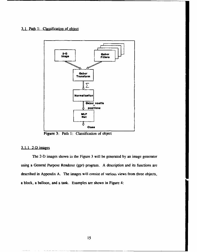
Figure 3: Path 1: Classification of object ......................... 15

Figure 4: Examples of objects ................................. 16

Figure 5: Position invariance example ........................... 18

Figure 6: Determination of perspective view ....................... 21

Figure 7: Gabor transforms of the block, balloon, and tank ............. 25

Figure 8: Position invariance test, theta = 450 ................. 26

Figure 9: In-plane test, theta = 450 ................ ............... 27

Figure 10: Out-of-plane test, theta = 45 ............................ 27

Figure 11: Position test, theta = 150 .......................... 29

Figure 12: In-plane test, theta = 150 .......................... 29

Figure 13: Out-of-plane test, theta = 150 ....................... 30

Figure 14: Position test, no summation ............................ 31

Figure 15: In-plane test, no summation ........................... 32

Figure 16: Out-of-plane test, no summation ........................ 32

Figure 17: In-plane test, set 2: no summation ....................... 33

Figure 18: Out-of-plane, set 2: no summation ....................... 34

Figure 19: Twist angle: similar test data ......................... 36

Figure 20: Twist angle: different test data ........................ 37

Figure 21: Camera's position: similar test data ...................... 38

Figure 22: Balloon shadings ............................... 41

V

Figure 23: Lighting positions................................. 42

Figure 24: (pr process..................................... 46

Figure 25: Tank.rle....................................... 54

Figure 26: Tank 1. rle: repositioned............................. 55

Ai

Lis f ales~

Table I: Geometry File Syntax (8).............................. 51

Table 11: Control File Syntax (8)............................... 52

Table III: Out-of-Plane test data............................... 56

Table IV: In-Plane test data.................................. 57

Table V: Out-of-Plane test data2............................... 57

Table VI: In-Plane test data2................................. 58

Table VII: Twist angle test coordinates........................... 58

vii

List of Text Boxes

1: Numerical approximation test: Wx window...................... 39

2: Numerical approximation test 2: 32032 window.................... 40

3: Shading test.......................................... 41

4: Lighting test.......................................... 42

5: Symmetrical test ....................................... 43

6. Sample control file...................................... 47

viii

Abstract

A different approach to pattern recognition was attempted using Gabor features,

artificial neural nets, and an image generator. The Gabor features and artificial neural

nets are sound biological-based, and the image generator provides complete access to any

view of an object. This research tested the idea that their integration could form a robust

3-D recognition system.

The results of the research showed that the Gabor features together with a neural

net were used successfully in classifying objects regardless of their positions, out-of-plane

rotations, and to a lesser extent in-plane rotations. The Gabor features were obtained by

correlating the image with Gabor filters of varying orientations spaced 150 apart as found

in primates' visual systems, and the correlation with each filter was kept separately.

ix

MODEL-BASED 3-D RECOGNITION SYSTEMUSING

GABOR FEATURES AND NEURAL NETWORKS

1. Introduction

The ability to recognize objects in a scene has great importance in military and

industrial applications. The problem is complicated by requiring the system to be

invariant to the object's position, scale, orientation, background noise, or occlusion. To

date, recognition systems have successfully addressed a few of these issues. However,

no single paradigm has solved all levels of the problem. (11:313)

The recognition process consists of segmentation, features extraction, and

classification. First, segmentaticn involves separating the regions of interest from the

background. Second, important features pertaining to the objects are extracted to reduce

the amount of information necessary for processing. Finally, the classification process

involves using these features to identify the objects. (18)

1.1 Backound

The Air Force Institute of Technology (AFIT) has on-going projects in all aspects

of the recognition problem. Among the most successful segmentation schemes

investigated at AFIT is the Gabor transform. Ayer showed that sine wave Gabor

functions acted similar to edge detectors, and cosine wave Gabor functions filled in the

I

body details. By combining both functions, complete segmentation (edge detection with

details) of FLIR images was accomplished. (2)

Two feature spaces were extensively researched at AFIT. The Kobel-Martin-

Horev (KMd) algorithm showed that targets could be located in a high clutter

environment through correlation of the transformed scene and template (20). Patterned

after similar work done by Casasent and Psaltis, this feature space was made invariant

to position, scale, and in-plane rotation (5). Another feature space used was invariant

moments (ordinary and Zernike). The moments were calculated for each object using

equations derived by Hu and Teague (15; 33) and fed to a decision rule for classification.

Robinson and Ruck demonstrated the usability of these features in their optical and

artificial neural network systems, respectively (25; 30).

Artificial neural networks as classifiers have been investigated predominantly in

the past several years. Both Troxel's and Ruck's implementation of multilayer perceptron

networks have shown great accuracy in classifying targets (34; 30). Presently, research

involves investigating different types of neural networks including Kohonen, Radial Basis

Functions, and Higher-order networks.

With respect to developing a recognition system that is invariant to orientation,

the above techniques have only addressed the in-plane rotation and su.ale problem.

Recognition of objects with respect to out-of-plane rotation is unsolved. This

thesis will research a solution to identifying objects regardless of their orientations (in or

out-of-plane rotations).

2

1.3 Assumtions

In order to limit the scope of the project, two assumptions are made. First, the

object of interest is already segmented. The segmentation problem can be resolved by

using the Gabor transforms as described in Ayer's thesis (2). Second, the range to the

object is known. This information can be obtained from using range data.

The recognition of the object will be accomplished in five steps (see Figure 1).

First, the Gabor features will be extracted from the 2-D image. Several Gabor templates

with varying orientations will be used. The sum of these templates will be reduced to a

more manageable size by retaining only the highest information content Gabor

coefficients. The reduced Gabor vector will be fed into a multilayer perceptron network

to determine the object's class in step two. The network will use the back-propagation

learning algorithm, and the training data will consist of reduced Gabor vectors of

different perspective views of the objects.

In step three, the determination of the object's perspective is achieved. Once a

class is determined, the same reduced Gabor vector will be fed into another multilayer

perceptron network. The training data will be similar to those used in step two except

the desired outputs are coordinates of the object's orientation. In step four, these

coordinates are entered into an image generator to produce a 2-D image with the

estimated orientation. The image generator contains a 3-D model of the object and can

generate any 2-D views of that object. Finally, in step five, the 2-D generated image

will be correlated with the original 2-D image to determine a Figure-of-Merit (FOM) for

3

the classification of the object in step two. A max FOM of 1 indicates that the generated

image is very similar to the original image.

2-D Qabor 2 Neural CiaseI m .ge Transeform Net

Neural

Generator

Correlaston

'4 FOM

Figure 1: Research approach

This chapter has provided a brief background on the work done at AFIT on a

recognition system, the problem, assumptions, and an outline of the approach used to

investigate the problem. Chapter HI provides the background information on related

rescarh in solving the recognition problem. Chapter III describes the detail processes

of the outlined approach. The results and discussions are in Chapter IV, and Chapter V

reviews the research with concluding remarks and recommendations.

4

11. Literature Review

Real-world image recognition remains a challenging problem for researchers in

the field. A robust recognition system must be able to identify objects in the scene

regardless of their positions, scales, or orientations (in-plane and out-of-plane rotations).

Given a two dimensional image, the system needs to extract important features from the

objects and use them for classification. Some of the feature extractors are biologically

based and are used successfully for identifying objects in their specific applications. The

addition of neural networks to approximate solutions to problems through adaptation and

learning provide for more robust and fault tolerant classifiers (21; 32). The combination

of a feature extractor and neural network may provide an applicable recognition system

for the non-linearity of real-world images.

This chapter will discuss several of these feature spaces: space-variant, moments,

and Gabor. Related studies in neural networks are presented. Finally, many 3-D

recognition systems require extensive storage space for various views of the object. A

model-based approach to alleviate some of the computational and storage burden will also

be discussed.

2.1 SMce-variant features

In 1977, Casasent and Psaltis proposed a feature space that is invariant to position,

scale, or in-plane rotation. This feature space could be used for correlation without loss

in signal-to-noise ratio of the correlation peak. Using the Fourier-Mellin properties, they

performed the Fourier transform of the scene to obtain position invariance, polar

5

coordinate transform to obtain rotation (in-plane) invariance, and logarithmic transform

to the radial axis to achieve the scale invariance. (5:77-84)

Following a similar approach, students at AFIT developed an algorithm (KMH),

Figure 2, that allowed for the determination of the correlation peak location and

subsequent identification of the target. The unique features of this algorithm were the

extraction and reinsertion of the phase information which contains the target's positional

information. Digital implementation of the algorithm proved successful in recognizing

multiple targets in non-random noise corrupted scenes. However, the computational time

was intensive and was considered infeasible for a real-time system. (14; 20)

Optical implementation by subsequent AFIT students proved useful (23; 6; 7), but

a number of problems remained in obtaining a real-world image recognition system. The

optical implementation of the phase extraction and reinsertion has not been realized.

Also, both the KMH and Casasent/Psaltis algorithms did not take into account the out-of-

plane rotation problem which is critical in real-world images.

To obtain out-of-plane rotation invariance, Schils and Sweeney proposed the use

of a small bank of optical correlation filters that can recognize objects from various

perspective views. The holographic filters are generated through iterative procedures.

An object is decomposed into a set of fundamental image components. These components

called eigenimages contain the essential information from all of the object variations.

This fundamental image information is then multiplexed, using phase, into each

holographic filter. Detection of target is based on finding points of constant intensity in

the correlation plane. Using a bank of 20 holographic filters, they were able to recognize

a tank with 16 different perspective views. (31)

6

SCENE TEMPLATE(x,y) i t(x,y) I

(f.,) ILFOURIE TO I)1 TRNPOLAR T

8( f) TRANS l~e

s~f..,OI RADIAL T on,""f J

SNVERS FT

PEAK LOCATION

IRECTIFY TEMPLATE

LOG TO LINEAR

POLAR TO RECT

INVERSE FT

LOCATE TARGET

RECTIFIED 8ENE

Figure 2: KMH Algorithm

Casasent achieved the out-of-plane rotation invariance by Linear Discriminant

Functions (LDFs) calculated from training set images. A LDF Computer Generated

Hologram (CGH), consisting of gratings with various modulation levels and orientations,

7

is placed in the feature space. The location formed by the projection of these gratings

in the output plane determines the object class. (3:449)

2.2 Moment features

Another feature space widely used in pattern recognition is moments. The use of

image moment invariants for two dimensional pattern recognition application was first

introduced by Hu in 1962 (15). By using central moments, which are defined with

respect to the image centroid, the features are made position invariant. Scale invariance

is made through normalization. Derivations for rotation invariant moments were more

complex. Teague improved upon Hu's work by deriving a set of moments which are

based on Zernike polynomials. The normalized central moments were also used to

account for scale and position variances. The rotational effect on the moments was

shown to be a multiplication of a phase factor related to the angle of rotation and the

degrre of the moment. (33.926) These Zernike moments suffer from the same

information loss problems as ordinary moments described by Hu, but not from

information suppression or redundancy (1:705).

Dudani et al applied these ordinary moment features to aircraft identification.

Moment parameters calculated from Hu's equations were reduced to the five most

important feature components. These components were used for classification in both the

Bayes and Distance-Weighted k-Nearest Neighbor decision rules. With a test sample of

132 images from 6 classes obtained at random viewing aspects, they proved that their

decision rules worked better than the human counterparts in identifying the various

aircrafts. (10) At AFIT, Robinson's research showed a 95.5% accuracy in identifying

various objects using these invariant moments in an optical setup (25:25).

8

2.3 Gabor features

A promising feature space for pattern recognition which fits well with the

empirical studies of the visual receptive fields in cats is the Gabor's (11:314). Following

the work of Dennis Gabor on data compression in 1946, Turner applied the Gabor

functions to image processing and found that by using a non-self similar Gabor function,

detailed textural features were retained without sacrificing global features such as

periodicity and overall data structure (2:13-14).

The general functional form of the 2-D Gabor filter is (9:1173)

g(x,y) - exp(- n[(x-x )da' + (y-y)P]) (1)

x exp(-2zi[uo(x-x.) + vo(y-y.)])

This function describes a complex exponential windowed by a Gaussian envelope.

The Gabor transform of an image, i(x,y) is then (27)

f(xy) - (x,y) * g(x,y) (2)

or

F(fW) - I(f.,1) G*(f4J) (3)

where * denotes correlation and * denotes complex conjugate.

Flaton and Toborg applied the Gabor theory to their image recognition system

called the Sparse Filter Graph (SFG). Feature vectors were constructed from convolving

the image witk Gabor filters at different orientations and spatial resolutions. The

collection of these features is reduced to "Mini-blocks" to reduce computation time.

9

"Mini-blocks" are chosen from feature vectors with the highest informational content.

The reduction process involved measuring how different one jet is with respect to

another, or saliency. Saliency is described as (11:316)

(IJal * nno -li i vaIl

where P and P are two different jets. The recognition process involved an iterative

process of comparing the input block against those stored in a database. The highest set

of match values is deemed the correct response. The experiment carried out was

successful in identifying a tank with the correct orientation. (11)

The feature spaces discussed above reduce a large quantity of information from

an image to a more manageable size. In the past, recognition of an image involved a

slow iterative process of matching the image's features to known features in a database.

The advent of neural networks provides for a more rapid approach to classification of an

image through approximation, and they are more adaptable to variabilities in the input

features than past techniques. The next section will discuss related research in using

neural networks as classifiers.

2.4 Neural Networks

Formulated from biological research, neural networks provide a heuristic approach

to solving problems that could prove quite successful in the areas of speech a-,d image

recognition where conventional computers have failed (26). The successful uses of neural

networks as classifiers are well documented in literature.

10

Using a multilayer perceptron (MLP) with back propagation (BP) learning

algorithm, Khotansad et a! showed classification accuracy of 97% for targets and 100%

for non-targets (19). At AFIT, Ruck's uses of MLP achieved 86.4% accuracy in

classification of tanks, using Zernike moment invariants as features (30:5-4). Similar

results were obtained by Troxel's research using features derived from the KMH

algorithm (34).

Other uscs of neural networks to predict target rotation and to synthesize filters

are being investigated at the University of Dayton. Gustafson et al used a 5 by 5 array

around a correlation peak as inputs into a backpropagation-trained neural net. With a

training set of 50 vectors, they were able to predict the rotation angle with less than ±

2.80 error. The same correlation grid was also used to generate a near-optimum filter for

a rotated target. After 78 training cycles, the results showed the synthesized filters in

general were superior to a fixed filter. (13)

The next section describes the use of the model-based approach as an alternative

to storing numerous templates and filters for various views of an image.

2.5 Model-based

The model-based approach involves the storage of a 3-dimensional model. The

consideration to use a model as a tool for the recognition process has two advantages over

the common technique of storing a bank of templates or filters. One, the issue of

sufficient object representation is greatly reduced since any 2-D views can be generated

from the 3-D model. Two, the storage burden is also alleviated.

At AFIT, the model generating process employs two common techniques, cubic

spline and surface polygons. Cubic spline provides for a more accurate description of

11

a curve surface than surface polygons. However, the surface polygons technique requires

less computational time because the mathematical description is simpler. (35) For this

thesis, the surface polygon technique will be used to generate the models.

Though they seemed realistic, the models still do not represent the true "picture

of the world". For example, the interaction of light with an object is too complex to

model mathematically. One workaround is to use texture wrapping that simulates the

reflection of light off of the object. Another is the use of ray tracing where the reflection

of one ray is modelled mathematically. Ray tracing improves the way one simulates the

reflection of light, however, it requires an enormous amount of computer time. (35) The

modelling technology is continually being improved, and despite the lack of realism, the

models themselves still offer valid research tools for the recognition process since all of

the train and test data are generated from the models.

Casasent and Liebowitz applied this model-based approach to their optical

symbolic correlator. Utilizing the capability to generate on-line images at any

orientation, they were able to control the filters used in identifying the image. The filters

were linear combinations of several reference objects in one or more classes. The peak-

to-sidelobe ratio (PSR) filters were used to locate the objects, correlation filters were used

to classify objects, and projection filters were used to confirm the object class and

determine the object orientation. A test on two classes with varying orientations resulted

in approximately 80% correct recognition. (4)

2-6 Summ&W

A robust recognition system requires the capabilities to extract important features

from an image and correctly classify the object regardless of its position, scale, or

12

The three feature spaces discussed provide working algorithms to reduce the image

information to a more manageable size. Neural networks have shown to be flexible

classifiers in light of the variabilities in the inputs, and a model-based approach can be

used to reduce the storage space. The next chapter will discuss the uses of these items,

and how they integrate to form a robust 3-D recognition system.

13

III. Methodology

The approach discussed in Chapter I outlined five steps to be accomplished in this

thesis study (see Figure 1). Steps 1 and 2 comprise the first path of the thesis in which

the goal is to see how well the Gabor information can be used to discriminate among

classes. Gabor coefficients and their relative positions will be used as features, and a

neural network will be used for classification. The output of path 1 will be the

probability that a given object within an image belongs to a certain class. Steps 3, 4, and

5 comprise the second path of the thesis in which the goal is to determine the perspective

view of the object. The Gabor coefficients and their relative positions will once again

be used as features, but a sub neural network will be used to output the estimated

coordinates of the object. This sub neural net will be activated based on the winning

class in path 1. Using the estimated coordinates, the image generator will produce the

corresponding two-dimensional template that will be correlated with the original image.

The result of this correlation will be a figure-of-merit for the classification of the object.

This chapter provides specific details on how each path will be accomplished and

a summary on the entire process.

14

3.1 Path 1: Classification of object

Gbor Goeff r

I MLP7

.1.12D images

The 2-D images shown ia the Figure 3 will be generated by an image generator

using a General Purpose Renderer (gpr) program. A description and its functions are

described in Appendix A. The images wil! consist of various views from three objects,

a block, a balloon, and a tank. Examples are shown in Figure 4:

15

Figure 4: Examples of objects

These images will be correlated with several Gabor filters, ano the transform

results will be used to form training and testing vectors.

3.1.2 Gabor filters

In order to limit the scope of the study, several parameters relating to the Gabor

filter will be fixed for all filters. First, the spatial frequency will be fixed at I cycle per

Gaussian window. Second, the size of the Gaussian window will be kept constant for all

filters, and third, only sinewave Gabors will be used in this study. The decision to use

sine over cosine Gabors originated from the curiosity in studying the use of edge

16

information on classification. Ayer's research has shown that sine Gabors can be used

to find edges of an object (2) The only parameter that will change will be the

orientation. A bank of filters will be generated with the three constant parameters

discussed above but with different orientations. The values for the orientations will vary

based on experimental results.

3.1.3 Gabor transform

The program "gabortf 1.c" in Appendix D will generate the desired filters as well

as perform the Gabor transform. The transforms of an image with the bank of filters will

be added together in magnitude, pixel-by-pixel. Next, all magnitude values will be

converted to positive numbers. Mueller and Fretheim's research has shown that negative

Gabor coefficients carry equal importance (information content) as their positive

counterparts. (24) The Gabor coefficients will then be sorted in order of their

magnitudes, and a "number" of the top Gabor coefficients and their relative x-y positions

on the image will be kept as features, forming a vector. This "number" will vary based

on experimental results.

The next step will involved normalizing these numbers to prep.re them as inputs

into the neural net.

3.1.4 Normalization

The normalization process will involve both horizontal and vertical normalization.

In this context, horizontal normalization involves finding the relationship of values within

a single vector, whereas vertical normalization is finding the relationship of values among

the vectors.

17

For horizontal normalization, each vector will be recalculated to obtain position

invariance. The Euclidean distance will be computed for each coefficient's x-y position

to the position of the maximum Gabor coefficient.

(distance) zi - V(Xi - xM)2 + - y) 2 (5)

where i is the position number of a Gabor coefficient in an array of coefficients sorted

in ascending order by their magnitudes. An example of the position invariant algorithm

can be shown in Figure 5:

4

4

Figure 5: Position invariance example

Given two objects (blocks in this case) of equal size but in different positions

within an image, the Gabor wavelets will ring the same points on the objects since the

texture information is the same for both objects. Assuming that '1' corresponds to the

maximum coefficient, then the Euclidean distances from all other points are relative to

the position of the maximum coefficient. Shifting position only changes the x-y locations

of the coefficients, not the relative distances to the maximum coefficient.

18

After normalizing each vector horizontally, all vectors will be normalized

vertically. The means and standard deviations will be calculated for each feature with

respect to all the vectors, and each value will be normalized by the following equation:

(new) x, - (od x1 - (6)O i

where i represents the position of each feature within a vector. pi and oa are the mean

and standard deviation, respectively, for the ith position. The program "norm.c" in

Appendix D will perform this normalization step.

These normalized features will be the inputs into a neural net for classification.

The features will be arranged as coefficient, position, coefficient, position, etc.. Again,

the number of features used will vary based on experimental results.

3.1.5 Neural net

The neural net will be a Multi-layer Perceptron (MLP) using Back Propagation

(BP) learning algorithm. The make-up of the net will consist of one hidden layer and an

output layer with three nodes, one for each class. The number of hidden nodes will vary

based on the number of inputs chosen. The output is expected to be a probability that

the given inputs belong to a certain class. (28) The node (class) that wins will drive

which sub neural net is to be activated in path 2.

The net will be trained using the normalized features of ra'.dom views of the three

objects. The number of training vectors will vary based on the number of input features

19

chosen. Foley's rule suggested that the number of training vectors should be at least

three times the number of input features for each class. (28)

Test will be performed on designated data at every 100 iterations through the

training data. The test will cover three areas: position invariance, out-of-plane rotation

invariance, and in-plane rotation invariance. For position invariance, the test images will

consist of a sample of the images from the training data but with the objects shifted

within the images. For out-of-plane rotation test, the data will consist of images that the

net has not seen but will have the same scale as the training images. The data for the in-

plane rotation test will be a set of images from the training data with the objects rotated

in-plane.

A "correct" is given if the error from each output node is less than 20%.

Training will stop when additional training does not provide significant improvement in

the accuracy of the test data. At this point, the net parameters (weights and offsets) will

be saved for future use.

With a trained neural net, path 1 is ready for usage. Given an unknown 2-D

image, the Gabor transform will be performed, and its normalized features will be input

into the neural net. The output of the net will contain the winning node (class) that will

activate the corresponding sub neural net in path 2.

20

3.2 Path 2: Determination of perspective view

Normaliz Gabor data Clss

r F - I I"° I

coordo #orData mple%

Conversion generation(7 Va)

ImageGenerator

2-Dtemplate

Original Eorlto2-0 Corrlltlon

imageFOM

Figure 6: Determination of perspective view

3.2.1 Sub neural net

There will be three sub neural nets corresponding to the three classes under study.

A single sub neural net will be activated based on the winning class from path 1. The

sub nets will be Multi-layer Perceptron nets using back propagation learning algorithm.

Each net will have one hidden layer and an output layer with seven nodes, corresponding

to the seven parameters needed for the image generator to produce a 2-D image. The

parameters are the x y z coordinates of the camera, the x y z coordinates of the center-of-

interest (coi), ane. the twist angle of the object.

21

The training data for each net will consist of normalized Gabor information of

random views of its class. The number of training vectors will vary based on the number

of input features chosen. As in the net in path 1, the test data for each sub net will cover

the position, out-of-plane rotation, and in-plane rotation invariance.

3.2.2 Data conversion

The outputs of the net are designed to be between 0 and 1, and the inputs into the

image generator could vary between -1500 and 1500 as in the case of the tank.

Consequently, it will be necessary to convert the net output numbers to more usable

numbers expected by the image generator. The ranges for the outputs will vary between

the three objects based on the scales given in their geometry files. Therefore, each sub

net will have its own data converter. Among the seven parameters, the ranges will also

be different. For example, the x and y coordinates for the camera and the center-of-

interest (coi) can vary between a negative "max" and a positive "max", but the z

coordinates will vary from 0 to a positive "max". Negative z coordinates will not be

used since recognition will not be attempted for the bottom of a tank. For the twist

angle, the range from 0 to 1 will correspond to angles from 0 to 360 degrees.

The converted numbers will be used to create a control file for the image

generator to use in creating a 2-D template.

3.2.3 Image generator

As mentioned earlier, the image generator creates images using a General Purpose

Renderer program. With a 3-D model in its data bank, the image generator can create

a 2-D image from any view. In path 2, a 2-D template will be generated with the view

22

specified by the control file from the sub net. The command used to generate the

template is given in Appendix A.

3.2.4 Correlation

Correlation is used to determine the similarity between two objects. In this case,

the similarity test will be between a 2-D template and the original unknown 2-D image.

The correlation peak will be used as a figure-of-merit (FOM) for the classification of the

object in path 1. A maximum FOM of 1 means that the two images are very similar.

Given the task of classifying an unknown 2-D image, the determination process

for this research is as follows: first, the Gabor transform of the image will be taken, and

the normalized features will be fed into a trained neural net. The output of the net will

be a probability that the given object within the image is of a certain class. Next, using

the same normalized features and a sub net activated by the winning class, an image with

the estimated view will be generated. This generated image will be correlated with the

unknown image to obtain a FOM on the classification.

The next chapter will provide the results and discussions on the research.

23

IV. Results and Discussions

This chapter provides the results of the approach described in Chapter 1H in four

parts. Part 1 discusses the findings related to the first task of trying to classify the three

objects. Part 2 discusses the findings of path 2 which is to determine the perspective

view. In part 3, the problems concerning numerical approximation, modelling

parameters, and their effects on the gabor features are provided. Finally, a summary

of the findings is presented in part 4.

4.1 Path 1: Classification of obiects

4.AZ11LdaTa

The test data for path 1 are given in Table III and Table IV in Appendix C. Each

test area consists of 15 test vectors, five for each object. Specific coordinates for the

position invariant test data are not available since the test data were obtained using a cut

and reposition method as described in Appendix B. This method was used to keep the

object at a constant scale. Other methods to reposition the objects were tried that seemed

to retain the object size to the observer, but experimental data have shown that the Gabor

transform was very sensitive to even the slightest pixel differences and will give different

results. The cut and reposition method was the only one guaranteed to keep the scale

constant.

24

4.1.2 Rotation at 450

The Gaussian windows for all filters were arbitrarily chosen at 8x8 pixels. The

first set of orientation angles tested were (0,45,90,135). These angles were effectively

used in Ayer's research to segment FUR images. (2) The Gabor transforms of the three

objects are shown in Figure 7. Since the Gabor window was fixed and small compared

to the objects' sizes, the sine Gabors picked out the edges of the objects as well as some

internal areas as in the case of the tank and balloon.

Figure 7: Gabor tansforms of the block, balloon, and tank

25

The net was trained with 60 vectors for each objects. The number of input features were

set at 20, 10 Gabor coefficients and their normalized positions, and the number of hidden

nodes was set at 10.

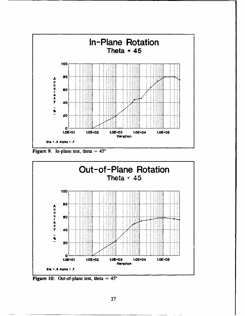
The results for the position, in-plane, and out-of-plane tests are given in Figure 8,

Figure 9, and Figure 10, respectively. The plots show accuracy of the test data versus

the number of iterations ran by the net.

Position InvarianceTheta * 45

100 :

8 ( .. o.... ........ .. .........; ,o................. i i i ... ... .i ....I ........ I.. ..A 8CC

- s o .....L... *. ....... •... .. .. . . ... ... ............. .. .... ............ ..

ra

2 0 --- ..... L . -i ' ---- ------ ....... .....I ...I

1.01E*Q1 1.0E*02 1.0E*03 1.0EP04 tLOE*06Iteration

Eta •.$ Alpha - .17

Figure 8: Position test, theta = 45°

26

In-Plane RotationTheta * 45

100----__-

A 8

a

y 40 --- 4 ...

0-1.OE+01 1.OE402 tOE+03 1.01E#04 1.OE#05

Iteration

Eta * .3 Alpha * .7

Figure 9: In-plane test, theta =450

Out-of -Plane RotationTheta At 45

100-

A 8

ra

40 ............

1.OE+01 1 OE+02 W.E.03 1 OE#04 1.OE+05Iteration

Eta - .3 Alpha - .7

Figure 10: Out-of-plane test, theta 450

27

As expected from the normalization method, the accuracy for the position

invariant test was very high. Of the 15 test vectors, there were no misses after 100,000

iterations, and given enough time, the accuracy percentage should be close to 100%.

The in-plane test gave good results with accuracy as high as 79.9% at 295,000

iterations, and the out-of-plane results were fair with accuracy reaching 58.4%. It was

difficult to draw any conclusions from these results at this point, except that they showed

promising steps in using Gabor features for classification. Further research indicated that

perhaps filters at every 150 orientation were more appropriate than at 45*. (16; 12; 17)

4.1.3 Rotation at 150

Hubel and Wiesel's work on the visual cortex indicated that certain cortical cells

responded best to lines with the right tilts, and the most effective orientation varies

between the range of 10 to 20 degrees. (16) Recently, Gizzi et al's research on the cat

striate and extrastriate visual cortex affirmed the fact that cells in both area 17 and the

lateral suprasylvian cortex (LS) response patterns are linked to the orientation of the

stimulus' spatial components. Using grating patterns, they found that the orientation

modal values for these cells were near 130. (12) AFIT's research has shown similar

results with moving grating patterns and found that the responses occurred at every 150.

(17)

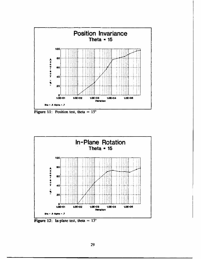
A new test was conducted with 12 filters at orientations 0" to 1650 spaced 150

apart. Again the net was trained with 60 vectors for each class, and the number of inputs

were set at 20. The results are shown in Figure 11, Figure 12, and Figure 13.

28

Position InvarianceTheta *15

100---_ _ -

A 0 ....... ... ......... . .- . .- . .......

U 60 ...... ... .... .. .. .......---

40 ........

20 .....

01.OE*0i tOE*02 1.OE.03 1.OE+04 1.OE+08

Eta * .3 Alpha * .7

Figure 11: Position test, theta 1 50

In-Plane RotationTheta *15

A100

U60

Y 0

1.01.01 1.0102 1.OE+03 .01.04 1.01.06

Et .8 Alpha - .7

Figure 12: In-plane test, theta 13I'

29

Out-of-Plane RotationTheta - 15

00

A- s o -........ .. .. .. ....... .... i .. .... ...C

'O !0 ..... ...... .... 0......

tI *1 tE02 tE0 .E0 .E0

11mationEta • .8 ph - .7

Figure 13: Out-of-plane test, theta = 150

The position invariant results once more gave high accuracy with no misses after

100,000 iterations. The accuracy for the in-plane test reached as high as 77.4% and for

the out-of-plane test, a 77.7% accuracy. There seemed to be an improvement in the out-

of-plane test, but no noticeable change was observed in the in-plane test. An observation

can be offered to explain these results. Perhaps, the summation of the Gabor transforms

could have diluted the information that is important to each filter. Another test with the

information for each filter kept separately seemed appropriate.

4.1.4 Rotation at 15: no summation

The orientation angles were again kept at 150 apart. The number of features

selected per filter was reduced to 10, 5 coefficients and their normalized positions. The

reduction in the selected features per filter was chosen to limit the number of inputs into

the net. The number five was chosen arbitrarily. The top five coefficients in magnitude

30

were selected from each filter. To avoid redundancy in information, if there was a match

in the coefficient's positions among the filters, the next highest coefficient was chosen.

The training vectors were increased to 416 for the block, 384 for the balloons, and

392 for the tank. With 12 filters, the number of inputs into the net was 120, and the

number of hidden nodes was increased accordingly to 60. The results are shown in

Figure 14, Figure 15, and Figure 16.

Position InvarianceTheta * 15

100s= o ....... i ii!... ~ iii...... .... 77 .A 6

U o ....... ........... i ii~

40l .......'i i i iil........i ... i i0

tOE+01 U.0E*02 1.0E+03 1.0E+04 10E06iteration

Eta - .3 Alpha - .7

Figure 14: Position test, no summation

31

In-Plane RotationTheta *15

100

A 80c

S 01

1.O1E*01 tOE*02 1.OE*0S 1OE*04 I.OE*05Iteration

Eta *.111 Alpha - .7

Figure 15: In-plane test, no summation

Out-of -Plane RotationTheta *15

100-

A 80....

U

y 0.. .. ........ ...... .......

1.OE#01 1.01E*02 tOE*03 tOE.04 i.OE.05Iteration

Eta - .11 Alpha - .7

Figure 16: Out-of-plane test, no summation

32

The same result was obtained for the position invariant test except the convergence

was much quicker as compared to previous results. The in-plane test gave comparable

results to those with the summation of the transforms. The out-of-plane test, however,

showed excellent results with accuracy as high as 92.6% at 57,600 iterations.

Another set of data was tested for comparison with the previous results. Table V

and Table VI in Appendix C show the coordinates, chosen randomly, for the in-plane and

out-of-plane tests, respectively. Again, the in-plane test gave similar results, Figure 17,to

the previous in-plane test data set. The out-of-plane results, Figure 18, did just as well

as the previous set with accuracy in the upper 90%.

In-Plane RotationTheta - 15

8 0 ......! ! i ii. ... .. . ............. .... ..........

0 so .... . . ... . . . . . .

. . ........ .-...-.................... . .20 ...... ...++++++~ i~+i+++++ + .......01

1.0E*01 1.0E*02 t0E*0$ t0E*04 1.0E*05lferation

Ets -. Aloft -. 1

Figure 17: In-plane test, set 2: no summation

33

Out-of-Plane RotationTheta - 15

100

8 0 .... ....l ........... . ........ i.. ..

u 0 ............. ...- .-................

4 0 ... " " '' ' ..... ....... ... r.:............ . .... r '"T"-,:: T ::: ........ -"'

2 0 . ... - - ------ - ...

tOE*01 1.0E*O2 11.E*08 1.0E*04 1.0E*06Iteration

Eta U.36 A-1s •.7

Figure 18: Out-of-plane, set 2: no summation

The similarty between the two sets of results increased the confidence that the net

was reporting accurately. The similar results of the in-plane test between keeping the

data separately and summation of the transforms were surprising considering the

normalization technique used. A review of the normalization technique described in

Section 3.1.4 showed that the technique provided not only position invariance, but also

in-plane rotation invariance. Since all distance calculations were relative to a maximum

coefficient's position, rotations in-plane should give the same summation results at any

orientation (in-plane).

If the summation technique provides for in-plane rotation invariance, why are the

results not in the upper 90%? The lower accuracy rates can probably be accounted for

by two reasons. One, as pointed out earlier, the summation of the tansforms could have

de-emphasized the important information while emphasizing the less important ones.

34

Two, error in numerical approximation of the Gabor transforms, which will be discussed

in more details in Section 4.3: Problems, seemed to be a likely contributor also. The

error in numerical approximation could have caused the same problem for the non-

summation technique in-plane test.

From the results, keeping the data separately for each filter at 150 orientation

seemed to offer the best results for classifying the objects in path 1. The same vector

format was used to determine the perspective view in path 2.

4.2 Path 2: determination of perspective view

Three tests were performed initially to see if the net could learn to output the

correct parameters necessary for the image generator to produce a template before moving

on to more complex tests as described in Chapter HI. Recall that these seven parameters

are the xyz coordinates of the camera, the xyz coordinates of the center-of-interest (coi),

and the twist angle. The first test involved only the twist angle with the test data taken

from the training data set. The second test again involved only the twist angle with test

data different from the training set. Finally, the third test varied the xyz coordinates of

the camera's position.

4.2.1 Twist angle: similar test data

The training set consisted of 360 vectors of a tank representing 360 degrees of in-

plane rotations. Again, the vector format was the same as those in Section 4.1.4 with

the data for each filter kept separately and the filter rotation at every 15c. The test data

was a subset of the training data. The results of the test are shown in Figure 19.

35

Perspective ViewTest Train, Twist angle

so .° ...............iii "i ii-A

u 0 ........... . ....... - ... . ....... .. ......... . .. . ... .

40 ..i'- ... - " - ... " ........... " .......0

1.011+01 tOE*02 1LOE0 1LOE*04 1.0OEO05Iteration

Elts - A Alph • .7

Figure 19: Twist angle: similar test data

The results showed that the net can output the correct parameter with excellent

accuracy. Of the 15 test vectors, there were no misses after 100,000 iterations, and given

enough time, the accuracy percentage should be in the high 90%.

4.22 Twist angeles different test data

Based on the results of the above test, the second test was performed with two

changes. One, it seemed unreasonable to train the net at every rotation angle (360) for

every view. This number was cut back to 24, 1 for each 15' of in-plane rotation. The

number of training vectors was also increased to 408 vectors of different views. The

second change involved the test data. The test data consisted of the same 2-D views but

with twist angles different from the training data (see Table VUI in Appendix C for the

listing of the parameters). The results of this test are shown in Figure 20.

36

Perspective ViewTest < Train, Twist angle

A.. ..Ui i i ...... .. ..... i ....... ... .i i i. ............ i i .i. ......... ......Y .. ...

2 0 ....... .. .. . ., , ... . ... . ... .. ...............

1.0E*01 1.0E*02 1.0E+O3 tOE+04 1.0E*05Iteration

Eta • .3 fth - .7

Figure 20: Twist angle: different test data

The results were very poor with the accuracy rate reaching only 34%. Several

runs were repeated with longer training time and different step size, eta, but the results

were similar. Two conjectures are offered to explain these results. One, the number of

training vectors per 2-D view, 24 in this test, were insufficient for the net to correlate

between the test data and the training data. The test in Section 4.2. 1 showed that the net

could learn with 360 training vectors per view. However, if further tests indicate that

a larger number, greater than 24, of training vectors per view is needed, the answer

would not seem reasonable since the number of training vectors would be enormous.

Two, a possible answer to the above results is that the MLP net with these vectors cannot

be trained to output the correct parameters within the error constraints. However, the

excellent results in Section 4.2.1 do not seem to support this argument. Further testing

would have to be performed to back up this answer.

37

mmmmm m mmm m m mm mmm mm a C

4.2.3 Camera's position: similar test data

This test involvd varying the xyz coordinated of the camera's position to see if

the net will output the correct parameters. Like Section 4.2.1, the test data was a subset

of those from the training set. The results are shown in Figure 21.

Perspective ViewTest -Train, Position's coords

100

A........... ....... ..............

u 4 0 ......-.....-.

2 0 ....... i i . .. ...0

1.0E*01 1.01[02 +1.0-$ 1.0E*04 41.0E.4.

Iteration

Eta - .4-.U Alpha * .7

Figure 21: Camera's position: similar test data

Similar to the last test, the results were poor with accuracy reach up to 35%.

Again, several runs were repeated, and the results were similar. These results seemed

to support the argument that the MLP net configuration with the Gabor features as

described cannot be trained to output the correct parameters within the error constraints.

No further tests as outlined in Chapter III were performed at this point since the

net cannot be used to provide the necessary parameters to generate a 2-D template. The

38

next section will discuss the problems encountered in this research, and their effect on

the Gabor transforms.

4.3.1 Numerical approximation

As indicated earlier, the numerical approximation of the Gabor transforms at

various angles were not consistent. Theoretically, a target at 0' with a Gabor filter at 0°

should give the same transform results as a target at any angle 6 with a Gabor filter at

the same angle 6. A test was performed to check this theory with one set at 00 and the

other at 250.

Gabor transform at 0: 15444 260 15444 1 15444 8 15444 119 15442 1

Gabor transform at 250 14899 395 14889 9 14315 1 14308 9 13788 102

1: Numerical approximation test: 8x8 window

Recall that the vectors' formats are coefficient, position, coeff, pos, etc., starting

with the highest coefficient. The first position is the summation of all the other distances

to the maximum position. From 1, the corresponding coefficients from both vectors are

slightly different. However, the corresponding positions in some cases are not even

close. This problem could have contributed to the lower accuracy rate in the in-plane test

since the Gabor transforms of various angles did not give the same theoretical results.

The errors in the numerical approximation are caused by the pixelized images

being used. Imagine a side of an object covering 5 pixels horizontally being rotate to an

angle where the side is aligned diagonally to the pixel array. The length of the side will

39

no longer be the same as the horizontal length, but it will be shorter or longer depending

on the modelling toc' used. When this problem is applied to an image, the picture at

diagonal rotation will be distorted, and with a small Gabor window (8x8 pixels), slight

differences will surface in the correlation results as seen from 1 above. The errors in

numerical approximation can be reduced by increasing the size of the Gabor window

where the correlation will take place over a larger area, and the slight differences will not

be as noticeable as shown in 2 using a 32x32 Gabor window.

(abor transform at 00: 12480 82 12480 1 12260 2 12248 1 12217 15

Gabor transform at 250: 1250668 12477 1 12311 1 122102 12115 15

2: Numerical approximation test 2: 32x32 window

4.21_ Shadinu

Different shadings have been found to give different results. For example, from

Figure 22. The balloon on the left was generated using FLAT shading, and the balloon

on the right was generated using PHONG shading. PHONG shading is generally used

on curve surfaces to provide smoother transitions between points on the curve, and FLAT

shading, as the name implies, is generally used on flat surfaces.

40

Figure 22: Balloon shadings

As seen from the Gabor transforms results in 3, the corresponding coefficients and

positions are slightly different. This problem gave varying results early in the research

but was eliminated by keeping the shading for each object constant for all of the training

and testing data.

FLAT: 15804 324 15795 9 12371 73 11993 73 11259 73

PHONG: 15804 887 15795 9 14671 115 14106 114 14060 114

3: Shading test

4.35L~ghting

Another modelling parameter that made a difference in the results was the position

of the fighting. An example is shown in Figure 23 with the lighting for the left block

from the camera's position and for the right block, from a point on the x-axis.

41

i !m

Figure 23: Lighting positions

The results in 4 again show slight differences in the numbers. For the entire test,

this problem was mitigated by putting the light at the camera's position.

camera's position: 15804 360 15795 10 15547 43 15368 45 15318 43

on x-axis: 15804 360 15795 10 15587 43 15522 45 15417 42

4: Lighting test

4.3.6 Symmetrical objects

An assumption was made early in the research that symmetrical objects will give

the same results at opposite points, and the training data need to cover only one quadrant.

However, as seen from the results in 5, this assumption should be made with a caveat.

The results came from two views of a block, one at coordinates (14.11,0,1) and the other

at the opposite side (-14.11,0,1). The slight differences in the numbers were not

understood, but the problem was mitigated by training in all applicable quadrants.

42

(14.11,0,1): 15804 217 15795 10 10996 1 10996 1 10987 9

(-14.11,0,1): 15804 394 15795 10 11362 47 10996 1 10996 !

5: Symmetrical test

In summary, the technique of keeping the transform data for each filter separately

provided the best overall results for classification of the objects. The position and out-of-

plane tests showed accuracy in the 90's, and the in-plane test showed accuracy in the

70's. Initial results for path 2 showed that the net could be trained to output the correct

twist angles. However, subsequent test with different test data gave poor results.

Another test to see if the net can output the correct camera's position also failed.

The problems with the modelling parameters and the numerical approximation

were discussed. The errors relating to the models were mitigated, but the symmetry

problem was not understood. The errors in numerical approximation were shown to

effect the Gabor transforms of the objects at various rotation angles.

The next chapter will discuss the implications of these results in the concl "-ions

section and will provide recommendations for further research.

43

V. Conclusions and Recommendations

5.1 Conclusions

A different approach to pattern recognition was attempted using Gabor features,

artificial neural nets and an image generator. The thrust of the research was to use an

image generator in the recognition process since it can generate any 2-D templates from

the 3-D model. This capability has the advantages of reducing the storage requirement

and providing sufficient knowledge over anyview of the object.

There were two major goals of this research: one, classify the objects using

Gabor informaticva and a neural net; and two, determine the perspective view of the

object to create a template for correlation with the original image. The results for the

classification of the objects were highly successful. Among the methods tested, the

technique of keeping the transform data separately for each filter provide the best overall

results. Repeated tests showed similar results and increased the confidence that the Gabor

features and the neural net can be used to classify objects.

Initial results with a change in one variable showed that the net can accurately

output the desired parameter. However, subsequent tests with increasing levels of

difficulty gave poor results. Further research need to be conducted before this

combination of MLP net and Gabor features can be dismissed as being unable to correctly

output the desired parameters.

Some modelling errors encountered during the research were discussed. Their

effects on the transform results were mitigated with respect to the experiments performed.

44

Future tests must reconsidered the effects of these and other parameters on that particular

research.

The numerical approximation error provides a possible explanation for the lower

accuracy rate in the in-plane tests. A larger Gabor window has been shown to reduce the

error, however, a possible trade-off could be less detail information given to the net.

There are four contributions provided by this thesis. One, the research showed

that Gabor features with a neural net can be used to classify objects regardless of their

positions, out-of-plane rotations, and to lesser extent in-plane rotations. Two, the use of

Gabor features and an MLP net to determine the perspective view of an image provides

initial direction for future study in accomplishing this task. Three, the understanding and

application of the image generator as a tool for pattern recognition have been advanced.

Finally, the fourth contribution of this thesis involved the identification of the problems

encountered during the research and provides "warning flags" for future research in this

area.

The next section will provide recommendations for future research.

5.2 Recommendations

1. Cosine Gabors could be used instead of sine Gabors or a combination of both.

2. The scale test was not performed in this research. The scale invariance could

be achieved by varying the Gaussian windows.

45

Appendix A: Image Generator

The images used in this thesis for testing were generated using a General Purpose

Renderer (gpr) developed at AFIT. Gpr is a general purpose polygon renderer written

in C++.

Gpr operates by rendering a geometry file which contains the specific coordinates

of the polygons and their attributes like textures and colors. The geometry model is then

rendered into an internal buffer based on the parameters specified in the control file.

These parameters include size of the image, coordinates that specify the perspective view

of the object, lighting, and background color. Once rendering is completed, the buffer

is written to an output file in Utah run length encoded (RLE) format. (22) (See Figure 24

below)

Figure 24: Gpr process

Rendering in this context is described as the transformation of a geometric description

into an image.

A. I Creating an image

As discussed above, the creation of an image requires both the geometry and

control files. The coordinates of the geometry model can be input directly if known or

46

generated using the commands: revolve and/or sweep. These commands generate

polygonal surfaces based on given profiles and paths of travel, and the outputs of which

are geometric description (coordinates and attributes) of the object. Complex objects can

be constructed by combining simple models using commands: rotate, scale, translate, and

combine. (See manual pages on the Sun for more detailed instructions) The geometry

file syntax is given in Table I.

The control files can be patterned after existing ones with modifications to certain

controlling parameters relevant to pattern recognition. (See 6 below)

buffer ABUFFER size 128 128 background 0 0 0vicwpo 0 127 0 127 ka 0. color I I Inumcameras I numlights 1

position 20 20 20 coi 0 0 0 twist 0 near 0.1 far 10000.0 fovx 50 fovy 50

direction 20 20 20 color I 1I1 status ON type INFINITE

6. Sample control file

The size of the images generated were kept at 128x128 pixels to minimize the calculation

time yet maintain enough resolution for visual display. The size can be adjusted by

changing the numbers on the first line of the control file. Note that an increase in size

will also increase the processing time (doubling the image size will increase the

processing time by 4). The perspective view of the object is set by changing the

coordinates of the camera's position, the center of interest (coi), and the twist angle. The

coordinates are arranged as x y z, and the twist angle is in degree of rotation about the

47

line of sight from the camera's position to the center of interest. These seven numbers

are the most important parameters relative to the pattern recognition research since they

control the perspective views (in-plane and out-of-plane rotations) of the object as well

as their relative sizes and positions. The last line specifies the lighting profile. The

direction of the light was kept from the camera's coordinates to the coi's coordinates.

Research has found that changing the light direction can affect the Gabor transforms as

indicated in Chapter IV. The remaining parameters in the file control other lighting

characteristics, colors, and the field of view which can remain unchanged. Table II

contains the control file syntax.

The following steps show how a balloon model and image are created:

=Vp1: Generate a profile

The coordinates are obta;.,d by plotting the profile of the object on graph paper

and creating a profile file with these numbers. The first line of the file specifies the

number of points to be plotted from the profile. In this example, there are eight points.

The next eight lines define the points further in three dimensional space. The format of

this definition is x y z Af nk n, where fi, fl., and k1 are the corresponding normals.

An attribute line follows with description of shading for the polygon surfaces.

< balloon.pro >

points 81 0010O0 (x y z n niy fio)100.75 1001.5 0 1.5 1 0 -0.52.502.5 10-1

48

3031002.504100.51.25 0 4.9 0.1 00.9005001shading FLAT reflectance FLAT kd 0.1 ks 0.3 n 10 color 1 00 opacity 1

NOTE: Addition information for texture can be included in the file but is omitted for

simplicity. See line 6+ of Table I for the syntax of the shading parameters.

so 2: Create geometry file

using command:

revolve < filename.pro > sector" degree > < outfile.geom >

revolve balloon.pro 20 18 > balloon.geom will rotate the balloon profile about

the z axis creating 20 sectors spaced 18 degrees apart.

go 3: Generate control file

a. Generate a file similar to the file in 6

b. Change the relevant parameters as discussed above

< balloon.control >

buffer ABUFFER size 128 128 background 0 0 0viewport 0 127 0 127 ka 0.1 color 11 1numcameras 1 numlights I

position 20 20 20 coi 0 0 0 twist 0 near 0.1 far 10000.0

fovx 50 fovy 50

direction 20 20 20 color 1 1 1 status ON type INFINITE

This control file will limit the image size to 128x128 pixels, and the object will be

viewed from the coordinates (20,20,20) to the center of interest (0,0,0) with no twist.

gI Generate RLE file

using command:

gpr -c controlfile -g gometryfile -o outputfile [-I listfile [-i infolevel]

49

where - specifies a list of geometry files to be rendered, and -i specifies the amount of

debugging information to be displayed. The -1 and -i flags are optional.

gpr -c balloon.control -g balloon.geom -o balloon.rle will create an image in

the file < balloon.rle >.

The RLE files can be displayed on several workstations:

TAAC gettaac < filename.rle >

SUN getsun <filename.rle>

SGI 4D get4D <filename.rle>

SGI 3130 getiris <filename.rle>

50

Table 1: Geometry File Syntax (8)

Line Keywords Description

I comments Anything up to 1024 characters

2 [ccwJ [cwl [purge] [nopurge] Geometry Parameters

3 + points <# of points> Object component/attribute countspatches <# of patches>(parts < # of parts > < list>](bsp < #of nodes>]I[attributes < # of attributes>][textures < # of textures>]

4+ <x> <y> <z> Vertex lines(normal <i> <j> <k>](color <r> <g> <b>][tindex <u> <v>]

5+ <n> <pt1> ... <pt n> Polygon/Patch lines(attribute < n >[texture < n>J][type {PLAINCOLOR ,TEXTURESTEXTIJRE)J

6+ [shading{FLAT,PHONG}] Attribute Lines[reflectance{FLAT,PHONG,COOK}](kd <n>] diffuse component(ks <n>] specular reflection component[n <n >J specular profile co!~o(opacity < n > < 1.0 for transparent surfaces[color <r> <g> <b>] base color of object[m <n >1 microfacet orientation distribution[material < filename >] name of material file

7+ [filename] texture map filename(WOODGRAIN < scale value > Isolid texture parameters

51

Table H: Control File Syntax (8)

Line Keywords Description

[buffer{ABUFFER,ZBUFFER, Buffer SpecificationSZBUFFER}][size <xsize> <ysize>] desired picture size[background <r> <g> <b >] background color

2 [viewport < vxl > < vxr > < vyb > Global Environment Parameters<vyt>][ka <n >] ambient light coefficient[color <r> <g> <b>] ambient light color

3 [numcameras < n > number of cameras[numlights < n > ] number of lights

4+ [position <x> <y> <z>] Camera Lines[coi <x> <y> <z>] center of interest[twist < n >] twist angle[near < n >] distance to near clipping plane[far <n>] distance to far clipping plane[fovx < n > field of view in x[fovy < n > field of view in y

5+ [position < x> <y> <z>] Light Lines[direction <i> <j> <k>] direction light is pointing[color <r> <g> <b>] color of fight[status{ON,OFF}] turns light ON and OFF[type{INFINITE,POINT,SPOT}] type of light source[exponent < n > specular profile[intensity < n > ] strength of light source[solidangle < n > spread angle for POINT and SPOT

Lights and COOK shading model

52

Appendix B. Repositioning Method

The data used for the position invariant test were obtained using a cut and

reposition method. For the test, the data needed to consist of objects in different

locations within the image while maintaining the same scale. Of the various methods

tried, the cut and reposition method was the only one that could accomplished this task.

The cut and reposition method employs four commands:

rlebg - create a background

crop - segment the object

repos - reposition the object

comp - combine the repositioned object with the background

BR-AI amp

The following steps show how a tank is moved to a new location while keeping

the scale constant:

s I Create a background

A background is generated to place the object on after it is repositioned.

Using the command:

rlebg red green blue [alpha] [-1] [-v[top[bott,.za]]] [-s xsize ysize] [outfile]

rlebg 0 0 0 -s 128 128 > bg.rle creates a black background of 128x128 pixels

and gives the output to the file bg.rle. For explanation of the options, see the manual

pages on the Sun 4.

53

step2: Segment the object

Given an image in Figure 25, cut out the object as shown by the dotted lines.

Figure 25: Tank.rle

Using the command:

crop xmin ymin xmx ymnax. [infile] > outfile

crop 10 25 118 108 tank.rle > t.rle cuts out the object at xmin-10, ymin-25,

xmax-1 18, and ymax-1O8. These coordinates are determined by how large the original

image is. In this example, the image is 128x128 pixels.

go 3; Reposition the object

Let's supposed the new desired location for the object is in the bottom left comner

of the image.

Using the command:

repos [-p xpos yposJ [14 zinc yincl infile] > outfile

54

repos -p 0 0 t.rle > tl.rle moves the lower comer of the cut out area represented

by (xmin,ymin) to a new coordinates (0,0). Explanations of the options can be found in

the manual pages on the Sun 4.

s : Combine

By combining the repositioned object with the background, a new image is created

with a repositioned object having the same scale as the object in Figure 25.

Using the command:

comp [-o op] Aile Bfile > outfile

comp -o atop tl.rle bg.rle > tankl.rle will output the results in tankl.rle as

shown in Figure 26. Other op commands can be found in the manual pages on the Sun

4.

Figure 26: Tankl.rle: repositioned

55

Appendix C: Test Data

Table MI: Out-of-Plane test data

Vectors Position's coordinates

Test. 1 (9.77,9.77,3)Test.2 (0,-13.82,3)Test.3 (-7.71,-7.71,9)Test.4 (-10.91,0,9)Test.5 (6.28,6,28,11)Test.6 (19.92,19.92,5)Test 7 (0,-27.53,9)Test.8 (24.28,0,17)Test.9 (-15.71 ,-15.71 ,20)Test. 10 (-14.13,0,27)Test. 11 (724.87,850,600)Test. 12 (-401.95,587,1000)Test. 13 (-509.02,-800,550)Test. 14 (806.05,-775,125)Test. 15 (806.75,980,0)

.56

Table TV: In-Plane test data

Vectors Position's coordinates Twist angle

Test.l1 (8.89,0,-Il) 15Test.2 (-11.22,-7,-5) 30Test.3 (4.69,-3,13) 40Test.4 (-5.48,-!3,1) -20Test.5 (-8.37,9,7) 53Test.6 (23.28,-16,4) -15Test.7 (-22.67,-16,8) 45Test.8 (19.64,18,12) 20Test.9 (16.55,8,24) -60Test. 10 (-15.42,16,20) -27Test. 11 (-1156.61,300,0) -30Test. 12 (-1153.77,100,240) 15Test. 13 (988.87,-400,480) -20Tet. 14 (-801.54,600,720) -40Test. 15 (-374.58,700,960) 17

Table V: Out-of-Plane test data2

Vectors Position's coordinates

Test. 1 (10, 10,0)Test.2 (12.65,2,6)Test.3 (-9.54, 10,-3)Test.4 (-9.98,4998,41)Test.5 (8.66,5,10)Test.6 (23.97,15,2)Test.7 (19.85,19.85,6)Test.8 (-22.42,-5,19)Test.9 (17.02,-2,25)Test. 10 (-22.78,15,10)Test. 11 (853.68,-210,800)Test. 12 (-764.69,790,625)Test. 13 (-725.83,1000,313)Test. 14 (-558.56,-840,487)Test. 15 (990.20,650,210)

57

Table VI: In-Plane test data2

Vectors Position's coordinates Twist angle

Test. 1 (9.77,9.77,3) 15Test.2 (0,-13.82,3) 30Test.3 (-7.71,-7.71,9) 40Test.4 (-10.91,0,9) -20Test.5 (6.28,6,28,11) 53Test.6 (19.92,19.92,5) -15Test.7 (0,-27.53,9) 45Test.8 (24.28,0, 17) 20Test.9 (-15.71,-15.71,20) -60Test. 10 (-14.13,0,27) -27Test. 11 (724.87,850,600) -30Test. 12 (-401.95,587,1000) 15Test. 13 (-509.02,-800,550) -20Test. 14 (806.05,-775,125) -40Test. 15 (806.75,980,0) 17

Table VII: Twist angle test coordinates

Vectors Position's coordinates Twist angle

Test. 1 (439.57,-1000,0) 10Test.2 (439.51,-1000,0) 53Test.3 (1038.83,-500,0) 25Test.4 (1038.83,-500,0) 100Test.5 (1199.51,0,0) 5Test.6 (1199.51,0,0) 70Test.7 (1 133.52,500,0) 93Test. 8 (1133.52,500,0) 125Test.9 (783.49,1000,0) 7Test. 10 (783.49,1000,0) 26Test. 11 (332.57,-1000,300) 33Test. 12 (332.57,-1000,300) 97Test. 13 (1000.33,-500,300) 48Test. 14 (1000.33,-500,300) 113Test. 15 (1166.46,0,300) 277

58

Appendix D. Source Codes

59

** The following codes were used to run a MLP neural network *1

/* This is the main program that calls other functions to perform theneural net input, calculations, and outputs. */

/include "macros.h"#include < stdio.h >#include "globals.h"

void menu(float [],float [],float 0,float 0);void makeinput(float [],float [1),void rangen(int [);void feed(float [],float I,float [],float [],float I,float fl,float []);void backprop(float f,float [],float [],float [],float [,float [],float [],

float [],int *,float *);void savejams(float [l,float [],float [],float []);void initialize(float f,float [],float ],float i0);void test(float *,int *,int *);

mainO{int seq[VECTORS + BVECTORS + TVECTORS];int ij,iteration,num;

iteration = 0;correct = 0;test acc = 0;eta = ETA;initialize(wl ,w2,tl ,t2);makeinput(feats,classes); /* generate an array of inputs */while (iteration < 150000){

rangen(seq); /* generate random number */loopi(VECTORS + BVECTORS + TVECTORS){

iteration + +;Ioopj(FEATJRES) /* select a random vector *1

vectorjl = feats[idx(seq[i]-l,j,FEATURES)];loopj(OUTPUTLAYER) /* assign appropriate output */{

if ((j+ 1) = classes[seq[ij-lJ)desiredoutputo] = 1.0;

elsedesired-outputblj] = 0.0;

60

feed(yhidden,y_out,wlI,w2,tl ,t2,vector);/* check error every 100 iterations *if ((iteration % 100) ==0)

num = iteration;printf(" %d\n" ,iteration);test(&test_acc,&correct,&iteration);

backprop(vector,wl1,w2,tl ,t2,y_hidden,y_out,desired~output,&num,&eta);

saveparams(wl ,w2,tl ,t2);

I* This function randomly assigns values to the weights and thetas withvalues between -1 and 1

#include <time.h>include < stdio.h >

#include <math.h>#include "macros.h"

int rangen(int [0);

initialize(float wl[],float w2[],float tlfl,float t20)

int ij,sign;int seqi VECTORS +BVECTORS +TVECTORS];

srand((unsigned)time(NULL));ran~gen(seq);loopi(OUTPUT LAYER)

loop j(IAYER ONE)

sign = (int) pow((double) -1 ,(double) seqUl);w2[idx(i,j,LAYER ONE)] = rand() % 100;w2[idx(i,j,LAYERONE)] = sign *

(w2[idx(i,j,LAYERONE)J/100);

sign = (int) pow((double) -1 ,(double) seqbj]);t2[i]j = rand() % 100;t2[i] = sign * (t2IilOO0);

61

loopi(LAYER ONE)

loop j(FEATURES)I

sign = (int) pow((double) -1 ,(double) seqo]);wl[idx(i,j,FEATURES)J = rando % 100;

wl[idx(i,j,FEATURE-S)J= sign *(w1[idx(i,j,FEATURES)]/ 100);

sign = (int) pow((double) -1 ,(double) seqo]);tl[i] = rand() % 100;tl[i] = sign * (tl[i]/100);

1* This function reads in the data vectors and creates arrays for furtherprocessing *

#include <stdio.h>include "inacros.h"

makeinput(float featsfl,float classesU)

FILE *fp;int ij;char filename[20];float c,f;float vect[VECTORS*FEATURES] ,bvect[BVECTORS*FEATURESJ,

tvect[TVECTORS*FEATURES] ,testvect[TETS];float class[VECTORSJ ,bclass[B VECTORS] ,tclass[T VECTORS] ,testclass[TESTS];

loopi(VECTORS) 1* store block data and class ~

sprintf(filename,"../normdatalvectors. %d",i+ 1);OPENFILE(fp,filename,filename); 1* open vector files for ~

/* reading */

loop j(FEATURES) /* storing features ~

fscanf(fp, %f ",&f);vect[idx(i,j,FEATURES)] = f

fscanf(fp,"%f\n",&c); 1* storing classes *Clas(iJ = C;

62

fclose(fp);

loopi(B VECTORS) /* store balloon data and class *

sprintf(filename,. Inormbdatalbvectors. % d" ,i + 1);OPENFILE(fp,filename,filename); I* open vector files for *

1* reading */

loopj(FEATURES) 1* storing features ~

fscanf(fp,"%f *,&f);bvect[idx(i,j,FEATURES)] = f

fscanf(fp, " %f\n",&c); /* storing classes *bclassti] = c;fclose(fp);

loopi(TVECTORS) 1* store tank data and class *

sprintf(filenanie,"../normtdataftvectors. %d",i+ 1);OPENFILE(fp,filename,filename); 1* open vector files for *

1* reading */

loopj(FEATURES) 1* storing features *

fscanf(fp,"%f ",&f);tvectfidx(i,j,FEATURES)] = f

fscanf(fp, "%f\n",&c); 1* storing classes *tclass[ij = cfclose(fp);

loopi(TESTS) 1* store test data and class ~

sprintf(filename,". .Itestdataltest. %d",i+ 1);OPENFILE(fp,filename,filename); /* open vector files for *

/* reading */

loopj(FEATURES) I* storing features ~

fscanf(fp,"%f ",M);testvect~idx(i,j, FEATURES)] = f

fscanf(fp,"%f\n",&c); 1* storing classes *testclass[i] = c;

63

fclose(fp);

loopi(VECTORS) 1* combine all data and classes *

loop j(FEATIJRES)feats[idx(i,j,FEATURES)] = vect~idx(i ,j,FEATURES)]

classesli] = classli];

loopi(B VECTORS)

loop j(FEATURES)featsfidx(i +VECTORS,jFEATURES)] =bvectllidx(i,j ,FEATURES)];

classes[i +VECTORS] = bclass[i];

loopi(T VECTORS)

loop j(FEATURES)feats[idx(i + (VECTORS + BVECTORS),j,FEATURES)]

tvect[idx(i,j,FEATURES)];classes~i +(VECTORS +BVECTORS)] = tclass[i];

loopi(TESTS)

loopj(FEATURES)feats~idx(i + (VECTORS + BVECTORS, + TVECTORS),j,FEATURES)]=

testvect[idx(i,j, FEATURES)];classes[i + (VECTORS + BVECTORS, + TVECTORS)J = testclass[i];

1* This function provides a random selection of the input vectors usedto train the neural nets *

finclude < stdio.h >#include <time.h>#include "macros.h"

rangen(int seq[VECTORS + BVECTORS + TVECTORS])

int count=O,i, randnum;

64

srand((unsigned)time(NULL));while(cowit < (VECTORS + BVECTORS +TVECTORS))

randnum = (rando % (VECTORS + BVECTORS, + TVECTORS)) + 1;for (i =O;i <countji+ +)

if(randnum ==seqi) break;

if(i > =count)

seq[countj = randnum;count+ +;

1* This function takes an input vector and feeds it through the net usingaigned parameters and provides the calculated outputs.

Original author: Greg TarrRevised by: Phung Le *

include "macros.h"include < nath.h >

float calcy(float [ifloat fl,float fl,int,int);

feed(float y hiddena,float y outfl,float wlfl,float w2fl,float tlfl,float t2fl,float inputfl)

int i;

loopi(LAYERONE) /* propagate inputs thru first layer ~yhidden[iJ = calcy(input,wl ,tl ,i,FEATURES);

loopi(OUTPUT_-LAYER) I" propagate from first to output layer ~youth]l = calcy(yhidden,w2,t2,,i,LAYER_ONE);

float calcy(float xa7,float weightjIJ,float thetafl,int upper,int lower)

int i;float y;

65

y = 0.0; /* initialize output value */loopi(lower) /* calculate summation of inputs x weights */

y = y + (x(i] * weight[upper * lower +i]);

y = y + theta[upper]; /* subtract the offset, theta */if (y < 60 &&-y > -60)

y = 1.0 / (1.0 + exp (-y)); /* return output as a function */else i" of a sigmoid *1{

if (y > = 60) /* boundary conditions */y = 1.0;

if (y <= -60)y = 0.0;

return (y);

/* This function uses the recursive backpropagation training algorithmto update the weights and thetas

Original author: Greg TarrRevised by: Phung Le */

#include "macros.h"#define MAX le34

void dely(float [),float [],float l-);void delx(float [],float (J,float [],float f);

backprop(float xD,float wlfl,float w2],float tl[],float t2],float yhidden[i,float youtri,float d[],int *N,float *eta)

{int ij;float del.upper[OUTPUTLAYER],delIower[LAYER_ONE];f 1 o a t

new wl[LAYERONE*FEATURESJ,neww2[OUTPUTLAYER*LAYERONE];float new tl [LAYERONE],new_t2[OUTPUT LAYER];s t a t i c f 1 o a t

old wI[LAYER_ONE*FEATURES],oldw2[OUTPUTLAYER*LAYERONE];static float old_tl[LAYERONE],old t2[OUTPUTLAYER];

if ((*N) > 30000)

66

(*eta) = (float) .3;I* calculate error terms and adjust weights from hidden to output

layer */loopi(OUTPUTLAYER) I* initialize ~

loopj(LAYERONE)new _w2[idx(i,j,LAYER_ONE)] = 0.0;

del upperli] 0.0;new-t2[iJ = 0.0;

dely(y_out,d,deLupper); 1* get error terms to output layer *loopi(OUTPUTLAYER)

loop j(LAYER ONE)

new w2[idx(i,j,LAYERONE)] =w2[idx(i,j,LAYERONE)] +(( eta) * del upper[i] * yhiddenoj]) +(ALPHA * (w2[idx(i,j,LAYER_ONE)] -

old w2[idx(i,j ,LAYERONE)]));old wv2[idx(i,j,LAYE ONE)] = w2[idx(i,j,LAYER ONE)];

new-t2[i] t2[il + ((*eta) * del..ypper[i]) +(ALPHA * (t2[i] - old-t[])

old-t2[i] =t2[i];

loopi(OUTPUTLAYER) /* reassign w2 and tQ with updated values *

loopj(LAYER-ONE)

if(eI2ixijLYROE]>MXinew w2[idx(i,j,LAERONE)] = MAX

if (new w2[idx(i,j,LAYERONE)] < -MAX)new_w2[idx(i~j,LAYfER_ONE)] = -MAX;

w2(idx(i,j,LAYER ONE)] new_w2[idx(i,j,LAYER_ONE)];

if (new-t2[iJ > MAX) new-t2[i] MAX;if (new_t2(iJ < -MAX) new-t2[i] -MAX;t2[i] = new-t2[i];

1* calculate error terms and adjust weight from input to hiddenlayer ~

loopi(LAYERONE) I* initialize ~

67

loop j(FEATURES)new _w1Iidx(i,j,FEATURES)] 0.0;

del -lower[i] = 0.0;new-tliji = 0.0;

delx(y_hidden,w2,del upper,del lower); /* get error terms to hidden */* layer ~

loopi(LAYERONE)

loopj(FEATIJRES)

new _wl[idx(i,j,FEATURES)] wl[idx(i,j,FEATURES)J +((*eta) * del -lowerfil * xj) +(ALPHA * (wl[idx(i,j,FEATURES)] -

old wi (idx(i,j,FEATURES)]));old_wi l[idx(i,j,FEATURES)j = wi [idx(i,j, FEATURES)];

new-tl[i] tli i + ((*eta) * del-lower[i]) +(ALPHA * (tl~iI - old tl[ij));

old-tlfi] =tl[i];

loopi(LAYERONE) /* reassign wi and ti with updated values *

loopj(FEATURES)

if(eIlixijETRSj>MXinew -Wl[idx(i,j,FEATURES)] = MAXi new_wl[idx(i,j,FEATURES)] < -MAX;inew wl[idx(i,j,FEATURES) -MAX

wl[idx(i,j,EATURES)] = new-wlI[idx(i,j, FEATURES)];

if (new-tl[iJ > MAX) new tl[i] MAX;if (new tl~ij < -MAX) new tl~iJ -MAX;tl[i] = new thui];

void dely(float yII,float dill,float delupper[])

int i;

loopi(OUTPUTLAYER)delupper[i] y[i] (1 - y[il) *(d[i] - y[i]);

68

void delx(float yIII,float wfl,float del uppero,float dei-lowerO])

int ij;float sum;

sum = 0.0;loopi(LAYER ONE)

loopj(OUTPUTLAYER)sum =sum + (del_upperol * w[idx(i,j,OUTPUTLAYER)]);

del-lower[i] =y[i] * (1 - y[iJ) * sum;

/* This function checks the testdata and assigns the error as well asthe accuracy associated with the test *

#include "macros.h"#include <stdio.h>#include "globals.h"

void feed(float [],float [],float fl,float [],float [],float [I,float [1);int check-error(float [],float [j,int *);

test(float *test- acc,int *correct,int *num-check)

int ij,vector-sum;

vector-sum = VECTORS + BVECTORS + TVECTORS;loopi(TESTS)

loopj(FEATURES) 1* select a random vector ~vectorol = feats[idx(i +vector-sum,j, FEATURES)];

loopj(OUTPUT LAYER) /* assign appropriate output *

if (6j+ 1) ==classes[i +vector sum])desired outputU] = 1.0;

elsedesired outputU] = 0.0;

feed(y-hidden,y_out,wlI,w2,tl ,t2,vector);check-error(y out,desired-output,correct);

1* acc = total correctlnum check *

69

"'test-acc = (float) (*correct)/(((*num check)/ 100) *(TESTS));printf("acc: %f\n",*test-acc);

1* This function calculates and displays the error at the output layer *

#include "macros.h"#include <niath.h>

check -error(float yo,float do,int *correct)

int i;float err;float error[OUTPUTLAYER];

err = 0;loopi(OUTPUTLAYER)

error[i] = fabs((float) dlii] - yi)err + = SQR(error[i]);

err = 5*erprintf("%f ",err);if (effor[0] < .2 && error[1] < .2 && error[2] <.2)

(*correct) + +;printfQ' %d\n" ,*correct);

/* This function saves the neural net parameters (weights, offsets, layernumbers) for later use. *

#include "mnacros.h"#include < stdio.h >

savejparams(float wlfl,float w2fl,float tlfl,float t2[])

mnt ij;char select;FILE *fp;char filename[201 = "gabor.wgt";

1* printf("Save parameters? )

select = getcharO;

70

if (select = = Wn)exit( 1);

elseI

printf("\nEnter filename: )scanf(" %s" ,filename);*ICREATEFILE(fp,filename,filename);fprintf(fp,"%d %d %d \n",OUTPUTLAYER,LAYERONEFEATURES);loopij(OUTPUTLAYER,LAYERONE)

fprintf(fp," %f ",w2[idx(ij,LAYERONE)]);loopij(LAYER_ ONE,FEATURES)

fprintf(fp," %f ",wl[idx(ij,FEATURES)]);loopi(OUTPUTLAYER)

fprintf(fp," %f ",C[i]);loopi(LAYER_-ONE)

fprintf(fp,"%f ",zl);fclose(fp);

/* This function provides 9, menu for initializing or assigning existing

values to all weights and thetas *

#include < stdio.h >

void initialize(float fl,float [],float [],float fl);void readjarams(char [],float [],float U,float fl,float [I);

menu(float wlfl,float w2[],float tl[],float t2U)

int select;char filename[20];

printf("\n.MENU\n");printf("1. Initilize parameters \n");printf("2. Retrieve parameter file \n");printf("e. EXIT \n");select = getcharO;switch(select)

case We: exit(O);break;

case 'Y': initialize(wl,w2,tl,t2);break;

71

case '2': printf('\nEnter filename: )scanf(" %s" ,filename);readparams(filename,wl ,w2,tl ,t2);

break;

1* This function reads in parameter values from an existing file andassign them to the weights and thetas appropriately *

#include *macros.h"#include <stdio.h>

readjarams(char filenameU,float wl[],float w211j,float tloj,float t2fl)

int ij;FILE *fp;float tempi ,temp2,temp3,temp4;int. output nodes,hidden-nodes,input nodes;

OPEN -FILE(fp,filename,filename);fscanf(fp,"%d %d %d",&output-nodes,&hidden-nodes,&input-nodes);

1* assigning weight values ~loopij(outputnodes,hidden-nodes)

fscanf(fp,"%f ",&templ);w2[idx(i,j,hidden nodes)] = temp 1;

loopij(hidden-nodes, input nodes)

fscanf(fp,"%f ",&temp2);wIfidx(ij,input_nodes)] = temp2;

I* assigning theta values ~loopi(output nodes)

fscanf(fp,"%f ",&teinp3);t2[i] = temp3;

Ioopi(hidden nodes)

fscanf(fp,"%f ",&temp4);tl[i] = ternp4;

72

fclose(fp);

I* Global variables for the neural networkfloat y_ hidden[LAYERONE] ,y_ogut[OUTPUTLAYER];float vector[FEATURES] ,desired _output[OUTPUTLAYER];float wiELAYERONE*FEATURES],w2[OUTPUTLAYER*LAYER_-ONE];float feats[(VECTORS +BVECTORS +TVECTORS +TESTS) *FEATURES];float classes[VECTORS + BVECTORS + TVLCTORS + TESTS];float tl[LAYERONE],t2[OUTPUTLAYER];float dzidxj;float test-acc;float eta;mnt correct;

Convenient Macros for Perceptron Package

/*** MACROS **

#define MAXPlC 128#define Boolean int#define FALSE 0#define TRUE 1

/** Mask Definitions*/#define OFF 0.0#define ON 1.0

#define rloopi(A) for(i=(A)-1 ;i > =0;i--)#define rloopj(A) foroj=(A)-l ;j> =0;j--)#define rloopk(A) for(k =(A)-lI;k > =0O;k--)#define rloopl(A) for( = (A)-1; 1 > =0;1--)#define rloopm(A) for(m=(A)-l ;m > =0;m--)#define rloopn(A) for(n=(A)-l ;n> =0;n--)#define rloopp(A) for(p=(A)-l;p> =0;p--)#define rloopij(A,B) for(i=(A)-l;i> =0;i--) foroj=(B)-l;j> =0;j--)#define loopi(A) for(i =0;i< A; i+ +)#define Ioopj(A) foroj=j < Aj+ +)#define loopk(A) for(k =0;k <A;k ++)

73

#define loopl(A) for( = 0;< A;I+ +)#define loopm(A) for(m=0;m < A;m + +)#define Ioopn(A) for(n=O;n<A;n+ +)#define loopp(A) for(p =0;p < A;p + +)#define loopij(A,B) for(i=0;i <A;i+ +) foroj=O;j <B;j+ +)#define MALLOC(A,B,C,D) if((A=(C *)malo((B)*sizef(C)))= =NULL){\

fprintf(stderr, strcat(D,": insufficient memory\n"))\exit(- 1); )

#define CREATE_-FILE(A,B,C) if((A =fopen(B,"w")) ==NULL){\

printf(strcat(C,": can't open for writing - %s.\n", 24),B);\exit (-1); 1

#define OPEN_-FILE(A,B,C) if((A=fopen(B,"r")) == NULL){\printf(strcat(C,": can't open for reading - %s.\n", 24),B);\exit (-1); )

#define idx(I,J,N) (I)*(N)+(J)#define FEQ(A,B) ( ( ((A)-(B)) < 1E-6 )? 1 : 0)#define SQR(X) (X)*(X)

#define TRAIN 0#define TEST 1

#define VECTORS 416 /* corresponds to number of views of an object *1#define BVECTORS 384 /* number of views of balloon *#define TVECTORS 392 1* number of views of tank ~#define TESTS 15 /* number of test vectors */#define FEATURES 120 /* number of Gabor coeffs, positions, and class *#define OUTPUTLAYER 3 /* number of output nodes *#define LAYERONE 60 1* number of hidden nodes *#define ETA .5 1* gain term */#define ALPHA .7 1* momentum term ~

**The following codes were used to generate gabor filters andto nomn~alize the feature vectors *

DATE: 18 Jun 90DESCRIPTIONS: This function performs: 1) conversion of image filefrom RLE to double format, 2) gabor transform of the image, and3) reduction of gabor coefficients to top NUM_COEFF (defined in macros.h).

FILES READ: 1. image.rle - image file in RLE format2. image.sum - summation of gabor transforms

PILES WRITTEN: I. vectors - contains top NUMCOEFF gabor coefficients andtheir respective positions.

74

AUTHOR: Phung Le

#include <nialoch>#include <stdio.h>#include "macros-h"#include < math.h >

unsigned char *read -rleO;void transformo;

maino

FULE *fpl,*fp2,*fp3,*fp4; /* file pointers *int i,j,ncolors,rows,cols,num;unsigned char *tempfile;double *dblfile;double temp;char filename[15];

OPENFILE(fpl,"image.rle","image.rle"); 1* get image *

/* read rie file and return unsigned char file */

tempfile = read -rle(fpl ,&ncolors,&rows,&cols);MALLOC(dblfile,rows*cols,double, "dblfile");

loopij(rows,cols) 1* cast to double ~dblfile[idx(i ,j,cols)1 = (double) tempfilellidx(i ,j,cols)1;

fclose(fpl);

CREATEFILE(fp2,"image.dbl","imiage.dbl");

ioopij(rows,cols) /* write new double file *fprintf(fp2," %f\n" ,dblfile[idx(i ,j ,cols)]);

fclose(fp2);transformo; 1* performs gabor transform of image ~

75

DATE: 8 Jun 90

DESCRIPTION: This function performs the Gabor transform of an image andarranges the transforms with each Gabor filter separately.

FILES READ: 1. gabordatl - contains frequency, orientation, and widthof the Gaussian window

2. image.dbl - image file in 'double' formatFILES WRITTEN: vectors

AUTHOR: Eric FretheimHISTORY: revised by Phung Le and Al L'Homme

#include < stdio.h >#include <math.h>include < string.h >

#include < ctype.h >include 'macros.h"#include "fft.c"

#define FORWARD 1#define BACKWARD -1#define PI 3.141592653589793

void indexxo;

transformOIint low freq,highfreq,freq_.cnt;int maxrot,rotstep,rot;int width,length,number,count;int i,j,k,filter;int indx[MAXPIC*MAX_PIC];int x[NUMCOEFF],y[NUMCOEFF];static int indxfile[NUMCOEFF*NUMFILTERS];double z[NUMCOEFF];s t a t i c d o u b I ecoeff[NUMCOEFF*NUMFILTERS],pos[NUMCOEFF*NUMFILTERS];double e[MAXPIC*MAXPlC];int tempfile[NUMCOEFF];

double **a;double **b;

76

double **c;double **d;double *xtr;double rtemp, itemp;

char file-nanie[151;

FTLE *ofp,*gd;j=O;a= (double **)calloc(MAXPIC,sizeof(xtra));b =(double **)callo(MAXPlC ,sizeof(xtra));c=(double **)calloc(MAX_PlC,sizeof(xtra));d= (double **)l(M APIC,szeof(xtra));if(!a II !b I I c II !d) j=l1;for(i=O;i <MAXPIC;i + +)

aIl(obe*cfo(AXPCszo~obe)a[i] =(double *)calloc(MAX_PIC,sizeof(double));b[i]= (double *)calloc(MAXPIC,sizeof(double));c[i] = (double *)calloc(MAX _PIC,sizeof(double));

if(!a[iJ !b[i] !c[i] I !d[i]) j = 1;

if (j)

printfCEi-ror! Calloc can't allocate enough meniory\n");exito;

1* open data file for reading *

OPENFI]LE(gd,"gabordatl ","gabordatl ");fscanf~gd,u %d",&low_freq);fscanf(gd," %d" ,&highfreq);fscanf(gd,'%d*,&max-rot);fscanf(gd," %d" ,&rot step);fscanf(gd," %d",&widtb);fscanf(gd," %d",&lengtb);

gget_file(a,b,width,Ilength); I* get image file *filter = 0;

for (freqcnt = low_freq; freqcnt < high freq + 1; freqcnt+ +)

77

for (rot = 0; rot < = max-rot; rot+ = rot_step)

printf("Calculatmng Freq %d, Rotation %d -- ",frec~cnt,rot);

rotate(c,rot,width,length,freqcnt); /*generate Gabor filter*/

printf(M -- ");

loopij(MAXPIC,MAX_-PIC) 1* initialize arrays *{~/ to zero*d[illjl = 0;e~idx(i,j,MAX_PIC)] = 0;

printf(" transform -A\n");

fft2(c,d,MAXPIC,FORWARD); f* Fourier T of filter *loopij(MAXPIC,MAX_-PIC)

/* Image x (filter)* *

rtemp = clijUl * alilli] - bWflj * d~ilUl;itemp = di]ji * alillu] + c[i]U] * b[i]UI;cliii] = rtemp;dli]U] = itemp;

fft2(c,d,MAXPIC,BACKWARD); 1* inverse FT to get *1* correlation results */

loopij(MAX PIC,MAXPIC) 1* convert to + values *if (cli][j] < 0) cliUI] = cia

loopij(MAXPIC,MAXPIC)e[idx(i,j,MAXPlC)] = clilol;

indexx(MAXPIC*MAX PIC,e,indx); 1* sort coeff by magnitude *count= 0;number=0;if (filter > 0)

while (count < NUMCOEFF)Iloopi(NUMCOjEFF*filter) 1* avoid redundant info *

while (indx fileji] indx[MAXPIC*MAXPlC-numberl)

78

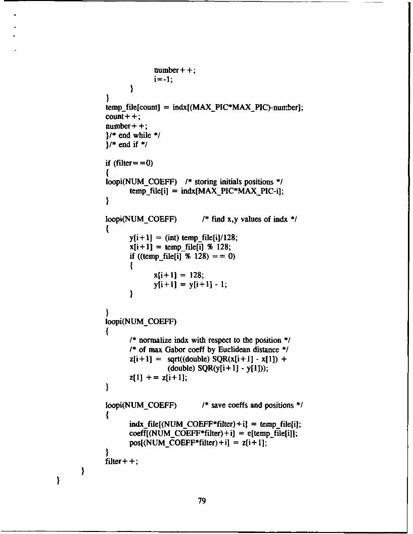
number+ +;

temp file~count] = indx[(MAX PIC*MAX-PIC)-numberJ;count+ +;number+ +;

}*end while */*end if */

if (filter = = 0)Iloopi(NUM_-COEFF) 1* storing initials positions *

temp fileli] = indx[MAXPIC*MAXPIC-i];

loopi(NUMCOEFF) 1* find x,y values of indx *

y[i+ 1] = (int) temp file[i]/128;x[i+1] = temp file~iJ % 128;if ((temp file[i] % 128) ==0)

x[i+1] = 128;yIi+1] = y[i+1] - 1;

loopi(NUMCOEFF)

/* normalize indx with respect to the position *1* of max Gabor coeff by Euclidean distance *z[i+l] = sqrt((double) SQR(x[i+1] - x[1]) +

(double) SQR(y[i+ 1] - yI~l]));z[1] += z[i+1];

loopi(NUMCOEFF) 1* save coeffs and positions ~

indxfile[(NUM-COEFF*filter) +i] = temp file[i];coeff[(NUMCOEFF*filter) +i] = e[tempfile[i]];pos[(NUMCOEFF*filter)+il = z[i+ 1];

filter+ +;

79

/* write out the file *

pritf("Ready to write )

CREATEFILE(ofp, "vectors", "vectors");

loopj(NUMFILTERS)

loopi(NUM-COEFF)

fpitIf,% fot of[*U -OF)i)fprintf(ofp,"%f "(float) coef[(*NUM COEFF)+ij);

fprmntf(ofp," % d\n", 1);fclose(ofp);printf("\nFile write complete\n");return;

gget,_file(real,imag,width,Ilength)double "ra;double **imag;in widtli,length;

double foo;int ij;FILE *fp;

fp = fopen("image.dbl", "r");

printf("File opened -- reading .\n");

loopij(MAX-PIC,MAXPlC)

fscanf(fp," %lf" ,&foo);real[iJjJl = foo;imagiill] = 0;

for (j = MAXPIC - length; j < MAX_PlC; j+ +)for (i = MAX PIC - width; i < MAXPIC; i+ +)

reallijiji = 0;

80

printf("Done reading - transforming .... n)

fclose(fp);

fft2(real,iinag,MAX PIC,FORWARD); /* FT of image *

return;

rotate(gab array ,degrees ,x size,y size ,omega)double **gab_array;int degrees, x size, y_size;int omega;

int ij;int l,m;double theta;double x,y,tx,ty;double xjprime,yjrime;double sig_x, sigjr;double gtfo;

theta =(((double) degrees) /180) *P1;

sig-x =x-size/8; /* covers +-4 standard devs *sigy =ysize/8;

loopij(MAX -PIC,MAXPlC)gab afraylilUl = 0;

tx = x -size;

ty = y-size;

for (j = y size/2; j < y size + y-size/2; j + +)for (i = i-size/2; i < x-size + x-size/2; i ++)

I =x size - iif (I < 0) 1 + = MAX-PIC;m = ysie- j;if (m < 0) m + = MAXPIC;X = j; y = j/* coordinates transformation *xprinie = x*cos(theta) - y*sin(theta)

- tx*cos(theta) + ty*sin(theta);yprime = x*sin(theta) + y*cos(theta)

81

- x*si(tkhet) - ty*cos~thet);

gab arrayll][in] = gtf(x~prime,yJprime,sig-x,sigj,,omega)*255;

double gtf(x,y ,sigiax,sigmay,cycles)double x,y;double signiax, sigajy;nt cycles;

double f-of-x;

f-of-x = (l/(2*PI*sigiax*sigmaj,))

*exp(JJ.5*((x/signp.-x)*(x/sigmax) + (ylsigmaj)*(y/sigma.y)));

f-of-x *= sin((x*PP* (double) cycles)/(2*sigmax)); 1* sine Gabor *

return (fofx);

/* This function performs the fourier transform of the given image *

#include "niacros.h"

fft2(picc ,ipicc ,n,dir)double **pjcc;double **ipjcc;int n;int dir;

dobepcMXPC 1double ipic[MAXPIC + I1;

int ij;

1* printf("Start Fourier transform --- rows.\n"); *

for (i =0; i < n; i ++)

for (j = 0; j < n; j ++)

82

fpicu+1I picctilo];ipic-U+ 1] ipicc~iJ]j];

fft(pic,ipic,n,dir);

for (j 0; j < n; j++)

picc[il picu+11;ipicc[i]U] ipicj+ 1];

for (I 0; j < n; j++)

for (i = ;i < n; i ++)

picli+1I picc[i][j];ipicli+1] ipicc[iJju];

fft(pic,ipic,n,dir);

for (i =0; i < n; i ++)

picciUl pic[i+ 1];ipicciUl ipic[i+ 1];

return;

fft(fr,fi,n,dir)double *fr;double *fj;int n;int dir;

double tr=0, ti=0;double wr=0, wi=0;double el=0, a=0;int i=0, j=0;int inr=0;

83

int 1=0;int k=O;int m=O, nn=O;int step=0;

if (dir < 0)for (i = 1; i < n+l; i++)

fi[i]=-fi]mrr=0;nn= n-i;for (m = 1; m <= nn; m++)

{1 = n/2;while (1 + mr > nn)1 = 1/2;mr = mr%l + 1;if (mr > m)

Itr = fr[m+ 1];fr[m+l] = fr[mr+l];fr[mr+l] tr;

ti = fi[m-t-l];

fi[m+1] = fi[mr+ 1];fi[mr+l] ti;}

}1=1;

while (I < n)Istep = 2*1;el = 1;for(m = 1; m <= 1; m++)

a = 3.1415926535 * (double) (1-m)/ el;wr = cos(a);wi = sin(a);for(i= m;i <=n;i +=step)

{j=i+l;

k =i;tr = wr*frUJ - wi*fiU];ti = wr*fiU] + wi*frUJ];frij] = fr[k] - tr;fi[J] = fi[k] - ti;

84

frlk] = fr[k] + tr;fi[k] = fi[k] + ti;

}

I = step;I

if ( dir < 0)for (i = 1; i < n+1; i++){

fr[i] = fr[i]/n;fi[i] -fi[i]/n;}

return;

rle.c: Routines to read and write RLE files.

Dennis W. Ruck, AFIT/ENGDS-90D

#include < stdio.h >#include < malloc.h >

#include < svfbglobal.h >#include "macros.h"

#define MAX-CHANNELS 4

unsigned char * readreO;void save_rleO;

unsigned char * readrle( image file, ncolors, rows, cols)FILE *image file;int *ncolors, *rows, *cols;{

Input: imagefile

85

Output: image, ncolors, rows, cols;

The routine will allocate memory for the image. Itis assumedthat the file has already been opened for reading.

unsigned char *image;rlepixel **scan;unsigned char *pixdata;int i, j, k, Incolors, rows, Icols, ro'-, y, offset;struct sv globals globals;

/** Read the header **/globals.svfbfd = image_file;rleget setup( &globals );*rows = Irows = globals.svymax-globals.sv_ymin+ 1;*cols = Icols = globals.svxmax-globals.svxmin+l;*ncolors = Incolors = globals.svncolors;

#ifdef DEBUGfprintf(stderr, "readne: image has %d rows and %d columns\

and %d channels\n", lrows, Icols, Incolors );fprintf(stderr,"readrle: xmin = %d, ymin = %d, xmax = %d, ymax =%d\n",

globals.svxmin, globals.svymin, globals.sv_xmax,globals.sv_ymax);

#endif

/** Allocate space for the image **if((image = (unsigned char *)maoc(lrows*lcols*lncolors))= =NULL){

fprintf(stderr, "readrle: insufficient memory, %d bytes requestedfn",frows*lcols*lncolors);

exit(-l);}if(rlerow alloc( &globals, &scan) ! 0)

fprintf(stderr, "readtie: insufficient memory\n");exit(-I);

}/ read in the image **/while( (y=rlegetrow(&globals, scan)) < = globals.sv_ymax) {

/** Transfer scanline information to image **// The returned image format has the channel information grouped in

contiguous memory by row major format starting at the top of theimage. Remember RLF returns information from the bottom of the

86

image first.row -globals.svymax - yloop(Incolors) I

offset = k*lrows*lcols;pixdata = scan[k];loopj(lcols) image[idx(row,j,lcols) + offset] = pixdata + globals. sv-xmin];

return image;

void save rle( image file, image, ncolors, rows, cols)

FILE *image file;unsigned char *image;int ncolors, rows, cols;

save -re: Routine to save image in an RLE format file. It isassumed the file has already been opened for writing.

riepixel **ca, *sros[A_CHANNELS];int i, j, k, offset;struct svglobals globals;

I** Set up the header **/globals.svfb-fd = image file;globals.sv~ymax =rows-i;

globals.svymin =0;

globals.sv -xmax =cols-l1;

globals. sv_xmin =0;

globals.sv -ncolors = ncolors;globals.sv_background = 0;globals.sv-comments = NULL;globals.sv-ncmap = 0;Ioopi(ncolors) SV_SET BIT (globals, i);sv _setup ( RUNDISPATCH, &globals);

if(rle-row-alloc( &globals, &scan ) ! = jfprintf(stderr, "save nie: insufficient memory\n");exit(-,);

87

/*save the image data*/loopi(rows) I

STransfer image information to scan /

I~The source image format has the channel information grouped incontiguous memory by row major format starting at the top of theimage. Remember RLE stores information from the bottom of theimage first.

loopk(ncolors)offset = k*rows*cols;srows[kJ = &image[idx((rows- 1)-i,O,cols) + offset];

svputrow( srows, cols, &globals)

/*put EOF mark*/svputeof( &globals)

/* This function sorts the data from the array 'arrin' in ascending orderand provides the order in the array 'indx' *

void indexx(n,arrin, indx)int nindx[J;float arrinO];

int l,j,ir,indxt,i;float q;

for (j=lI;j <=n;j ++) indxUj =j;if (n = = 1) return;1=(n > > 1) + 1;ir=n;for (;;) I

if (I> 1)q=arrin[(indxtindx[--])];

else Iq =arrnn[(indxtindx[irj];indx[ir] =indx[1;if (--ir == l){(

indx[1] =indxt;return;

88

j=l «1< ;while j < = ir)

if j < ir &&arrin[indxbj]] < arrinhindxU +I])ji++;if (q < arrmlindx~j]]) I

indx[iJ = indxlii;j+ = (i=j);

else j=ir+l1;

mndxli] = indxt;

1* This function normalizes the data vectors for further processing ~

#include < stdio.h >#include "niacros-h"#include <math.h>

void distribution(floatfl ,floatfl,float DI,int);

main()

FILE *fp,*fpl;int i,j,c;char filename[20];float f;float mean[FEATURES] ,cmean[FEATURESJ,bmean[FEATURESI,

tniean[FEATURESJ;float std-dev[FEATlJRESJ ,cstd-dev [FEATURES] ,bstd dev [FEATURES],

tstd-dev(FEATURES];float x-cube[VECTORS*FEATURESI ,x bulb [B VECTORS *FEAT URES],

xtank[rVECTORS*FEATUIRESI ,x[VECrORS*FEATURES];float feats[FEATURESJ ,classes[ VECTORS];float m[FEATURES],s[FEATURES];

loopi( VECTORS)

sprintf(filerame, "../data/vectors. %d",i+ 1);

89

OPENJFI E(fp,filename,filename); /* open vector files for *1* reading *

loop j(FEATURES)

fscanf(fp,'%f ",Mf);xcubeidx(i,j,FEATURES)] = f

fclose(fp);

distribution(m, s, x-cube, VECTORS); /* get mean & std dev *loop j(FEATURES)

cmeanlj] = ma];cstd-devU] = Q

loopi(B VECTORS)

sprintf(filename, ".. /bdata/bvectors. % d ",i + 1);OPEN FILE(fp,filename,filename); 1* open vector files for *

I* reading *ioopj(FEATURES)

fscanf(fp,"%f ",&f);xbulb[idx(i,j,FEATURES)] f;

fclose(fp);

distribution(m,s,x-bulb,BVECTORS); 1* get mean & std dev *loop j(FEATURES)

bmeanljl = mU];bstd-devUl] = s]

loopi(T VECTORS)

sprintf(filename,"../tdata/tvectors. % d" ,i +1);OPEN FILE(fp,filename,filename); 1* open vector files for ~

1* reading *loopj(FEATURES)

fscanf(fp," %f" ,&f);xtankidx(i,j,FEATURES)] = f

fclose(fp);

90

distribution(m,s,x tank,TVECTORS); /* get mean & std dev *loopj(FEATURES)

tmeanoj] = mojj;tstd_devoj] = s]

loopj(FEATURES) /* sum all means and std-devs *

meanoj] = cmeano] + bmeanb] + tmeanU];std_devol = cstd devojl + bstd-deviji + tstd-devUl;

CREATEFILE(fp,"mean.dat","mean.dat");CREATE7FILE(fpl , -std-dev.dat", "std-dev.dat");loopj(FEATURES) /* save means and std-devs *

fprintf(fp,"%f ",meanU]);fprintf(fpl,"%f ",std-devol);

fc o e f )fclose(fp);

loopi(VECTORS) 1* normalize all data by average max value ~

sprintf(filename,"../normdatalvectors. %d",i +1);OPENFILE(fp,filename,filename); /* open vector files for *

1* reading */loopj(WEATURES) /* storing features ~

fscanf(fp,"%f ",&f);featsl = f

fscanf(fp,"%d",&c); /* storing classes *classes[i] = (float) c;

fclose(fp);

loopj(FEATURES) 1* calculate new values *featsbj] = (featslj) - meanbj/std -devl;

CREATEFILE(fp,filename,filename) /* open file for writing ~

91

loop j(FEATURFS)fprintf(fp," %f ",featsojD;

fprintf(fp," %f\n" ,classes[i]);fclose(fp);

ioopi(BVECTORS) 1* normalize all data by average max value ~

sprintf(filename, ".. /normbdatalbvectors. % d" , i + 1);OPEN FILE(fp,filename,filename); 1* open vector files for *

I* reading */loopj(FEATURES) 1* storing features *

fscanf(fp,"%f ",&f);featsoj] =f

fscanf(fp,"%d",&c); 1* storing classes ~classes[i] = (float) c;

fclose(fp);

loopj(FEATURES) 1* calculate new values *featsU] = (featsl - mueano)/std-devo];

CREATEFILE(fp,filename,filename) 1* open file for writing *loop j(FEATURES)

fprintf(fp," %f ",featsj);fprintf(fp," %f\n",classesli]);fclose(fp);

loopi(TVECTORS) /* normalize all data by average max value *

sprintf(filename, ".. /normtdata/tvectors. % d", i + 1);OPEN FILE(fp,filename,filename); /* open vector files for *

1* reading */loopj(FEATURES) /* storing features ~

fscanf(fp,"%f ",&f);featsU] =f

fscanf(fp,"%d",&c); /* storing classes *classes[i] = (float) c;

fclose~fp);

loopj(FEATURES) 1* calculate new values *featsUl = (featsl] - meanUj])/std-dev~J;

CREATEPILE(fp,filename,filename) I* open file for writing *loop j(FEATURES)

92

fprintf(fp,-%f ",featsl);fprintf(fp," %f\n",classes[i]);fclose(fp);

void distribution(float mIa,float sfl,float values[],int size)

mnt i,j;float sum[FEATURES],suml [FEATURES];double varIIFEATURES];

loopj(FEATURES) /* initialize values *

suml = 0;sumloj] = 0;

loopj(FEATURES) I* calculate mean ~

loopi(size)suml] + = i'alues[idx(i,j,FEATURES)j;

ml = sumoj]/(VECTORS +BVECTORS+TVECTORS);

loopj(FEATURES) 1* calculate standard deviation ~

loopi(size)sumlUl + = SQR(values[idx(i,j,FEATURES)] - mU]);

varl] = sumloj]/((VECTORS+BVECTORS+TVECTORS) - 1);if (varol = 0) Suli = 1;else soj] (float) sqrt(varU]);

93

1. Abu-Mustafa, S. Yaser, and Demetri Psaltis. "Recognitive Aspects of MomentInvariants," IEEE Transctions on Pattern Analysis and Machine Intelligence. Vol PAMI-6. No 6:698-706 (November 1984).

2. Ayer, Capt Kevin W. Gabor Transforms for Forward Looking Infrared ImageSegmeltati n. MS Thesis, AFIT/GEO/ENG/89D-1. School of Engineering, Air ForceInstitute of Technology (AU), Wright-Patterson AFB OH, December 1989 (AD-A215046).

3. Casasent, David. "Scene Analysis Research: Optical Pattern Recognition andArtificial Intelligence," SPIE Optical and Hybrid Computing. Vol 634: 439-56 1986.

4. Casasent, David and Suzanne A. Liebowitz. "Model-based Knowledge-based OpticalProcessors," Applied Optics. Vol 26. No 10: 1935-42 (15 May 87).

5. Casasent, David and Demetri Psaltis. "New Optical Transforms for PatternRecognition," Proceedings to the IEEE, Vol 65. No 1: 77-84 (January 1977).

6. Childress, Capt Timothy G. and J. Thomas Walrond. Position. Scale. and RotationInvariant Optical Pattern Recognition for Target Extraction and Identification. MSThesis, AFIT/GE/ENG/88D-4. School of Engineering, Air Force Institute of Technology(AU), Wright-Patterson AFB OH, December 1988 (AD-A202600).

7. Cline, Capt John D. Hybrid Optical/Digital Architecture for Distortion InvariantPattern Reogilition. MS Thesis, AFIT/GEO/ENG/89D-2. School of Engineering, Air

Force Institute of Technology (AU), Wright-Patterson AFB OH, December 1989 (AD-A215628).

8. Dahn, Capt David A. "GPR User's Manual," Air Force Institute of Technology(AU), Wright-Patterson AFB OH, (14 July 1990).

9. Daugman, John G. "Complete Discrete 2-D Gabor Transforms by Neural Networksfor Image Analysis and Compression," IEEE Transactions on Acoustics. Sp ech. andSionl Processing. Vol 36. No 7:1169-79 (July 1988).

10. Dudani, Sahibsingh A., Kenneth J. Breeding, and Robert B. McGhee. "AircraftIdentification by Moment Invariants," IEEE Transactions on Computers. Vol C-26. No.L 39-45 (January 1977).

94

11. Flaton, Kenneth A. and Scott T. Toborg. "An Approach to Image Recognitionusing Sparse Filter Graphs," 1989 IEEE INNS International Joint Conference on NeuralNetworks, Vol 1: 313-20 1989.

12. Gizzi, Martin S., Ephrain Katz, Robert A. Schumer, and J. Anthony Movshon."Selectivity for Orientation and Direction of Motion of Single Neurons in Cat Striate andExtrastriate Visual Cortex," Journal of Neurophysiology. Vol 63, No 6e1529-43 (June1990).

13. Gustafson, Steven C., David L. Flannery, and Darren M. Simon. "NeuralNetworks with Optical Correlation Inputs for Recognizing Rotated Targets." Universityof Dayton, Research Institute, Dayton OH, 1990.

14. Horev, Moshe. Picture Correlation Model for Automatic Machine Recognition. MSThesis, AFIT/GE/EE/80D-25. School of Engineering, Air Force Institute of Technology(AU), Wright-Patterson AFB OH, December 1980 (AD-AI00765).

15. Hu, Ming-Kuei. "Visual Pattern Recognition by Moment Invariants," IMETransactions on Information Theory. IT-8: 179-87 (February 1962).

16. Hubel, David H. and Torsten N. Wiesel. "Brain Mechanisms of Vision," SinificAmerican. Vol 241. No 3; 150-163 (1979).

17. Kabrisky, Matthew. Personal interviews. School of Engineering, Air Force Instituteof Technology (AU), Wright-Patterson AFB OH, October 1990.

18. Kabrisky, Matthew. Lecture notes taken in EENG 620, Pattern Recognition I.School of Engineering, Air Force Institute of Technology (AU), Wright-Patterson AFBOH, 1990.

19. Khotanzad, A., J. H. Lu, and M. D. Srinath. "Target Detection using a NeuralNetwork-based Passive Sonar System," IEEE INNS International Joint Conference onNeural Networks. Vol I: 335-40 1989.

20. Kobel, Capt William G. and Timothy Martin. Distortion Invariant PatternRecognition in Non-Random Noise. MS Thesis, AFIT/GE/ENG/86D-20. School ofEngineering, Air Force Institute of Technology (AU), Wright-Patterson AFB OH,December 1986 (AD-A177598).

21. Lippman, Richard P. "An Introduction to Computing with Neural Nets," IEEEASSP Magazine 4-22 (April 1987).

95

22. Manual pages on Sun 4's pertaining to "gpr".

23. Mayo, 2Lt Michael W. Comuter Generated Holomms and Mdgueto-Optic SpatialLight Modulator for Optical Pattern Recognition. MS Thesis, AFIT/GEO/ENG/87D-1.School of Engineering, Air Force Institute of Technology (AU), Wright-Patterson AFBOH, December 1987 (AD-A 189553).

24. Mueller, Michael, Erik J. Fretheim, Matthew Kabrisky, and Steven K. Rogers."Gabor Transforms to Preprocess Video Images for Back-Propagation,"

25. Robinson, Capt Vicky L. Hybrid Calculation of Invariant Moments. MS Thesis,AFIT/GEO/ENG/88D-3. School of Engineering, Air Force Institute of Technclogy(AU), Wright-Patterson AFB OH, December 1988 (AD-A202594).

26. Rogers, Maj Steven K. and Matth-w Kabrisky. Biological and Artificial NeuralNetworks for Pattern Recognition. School of Engineering, Air Force Institute ofTechnology (AU), Wright-Patterson AFB OH, 1990.

27. Rogers, Maj Steven K. Lecture notes taken in EENG 527, Fourier Optics. Schoolof Engineering, Air Force Institute of Technology (AU), Wright-Patterson AFB OH,1989.

28. Ruck, Capt Dennis W. Characterization of MLP and their Application to Multi-sensor Automatic Target Detection. PhD Disertation, AFITiGE/ENG/DS-90D. Schoolof Engineering, Air Force Institute of Technology (AU), Wright-Patterson AFB OH,December 1990.

29. Ruck, Capt Dennis W., Steven K. Rogers, and Matthew Kabrisky. "FeatureSelection Using a Multilayer Perceptron," Submitted for publication in T JurInal fNeural Network Computing.

30. Ruck, Capt Dennis W. Multisensor Target Detection and Classification. MSThesis, AFIT/GE/ENG/87D-56. School of Engineering, Air Force Institute ofTechnology (AU), Wright-Patterson AFB OH, December 1987 (AD-A177598).

31. Schils, George F. and Donald W. Sweeney. "Optical Processor for Recognition ofThree-Dimensional Targets Viewed from any Direction," Journal of the Optical Societyof America A. Vol 5. No 8: 1309-21 (August 1988).

32. Tan, Capt Gregory L. Dynamic Analysis of Feedforward Neural Networks UsingSimulated and Measured Data. MS Thesis, AFIT/GE/ENG/88D-54. School ofEngineering, Air Force Institute of Technology (AU), Wright-Patterson AFB OH,December 1988 (AD-A202573).

96

33. Teague, ! lichael R. "Image Analysis via the General Theory of Moments," Jouralof the Optical Society of America. Vol 70. No 8: 920-30 (August 1980).

34. Troxel, 1Lt Steven E. Position. Scale, and Rotation Invariant Target Recognitionusing Range Imagery. MS Thesis, AFIT/GE/ENG/87D-3. School of Engineering, AirForce Institute of Technology (AU), Wright-Patterson AFB OH, December 1987 (AD-A188828).

35. Dahn, Capt David A. Personal interview. School of Engineering, Air ForceInstitute of Technology (AU), Wright-Patterson AFB OH, September 1990.

97

Vita

Captain Phung D. Le was born on 2 Feb 1964 in Da Nang, Viet Nam. He

immigrated to the United States in the summer of 1975 and lived in Illinois then

California where he graduated from Homestead high school in 1982. In June 1982, he

entered the United States Air Force Academy and received his commission in May 1986.

Upon graduation, he was assigned to the Ballistic Missile Office, Norton AFB CA, where

he was a Guidance and Control Project Officer. While there, he obtained a Master of

Science in Systems Management at the University of Southern California.

98

December 1990 Final-1. rIT'. AN tD 'U37;TL ' . '. I "_7- i . S

Model-Based 3-D _Recognition System Using

Gabor Features and Neural Networks

i. AUTHOR(SW

Phung D. Le, Capt, USAF

School of EngineeringAir Force Institute of Technology (AFIT)irignt-Patterson AFB, OH - -.33-6583

.. . .. U . .... . . . .. . ," - -.. .•" ,- " . . - ' 2 - ' - . - _ , : . - , ', - .,

Approved for public release; Distributionunlimited

A different approach to sattern recognition was attemted using Gaborfeatures, artificial neural nets, and an image generator. The Gabor

features and artificial neural nets are sound biological-based, andthe image generator provides complete access to any view of an object.This research tested the idea that their integration could form a robust3-3 recognition system.>he results of the research showed that the Gabor features together with

a neural net were used successfully in classifying objects regardlessof their positions, out-of-plane rotations, and to t lesser extentin-plane rotations. The Gabor features were obtained by correlatingthe image with Gabor filters of varying orientations soaced 1. degreesapart as found in primates' visual systems, and the correlation witheach filter was kept separately.

Fattern recognition, Gabor, Neural networks, :-odels 9',

Unclassified i Unclasified Unclassified UL(unliiteu)