pROGRAMMING lANGUAGE - se3 …se3-informatics.wikispaces.com/file/view/1- SE3 - Excel - Quiz 2... · Web viewWrite a formula to calculate the Tax of "Price to Pay before tax" of every

RHHS – SE3 - HUMANITIES EXCEL – Functions

Nested If A Nested IF function is when a second IF function is placed inside the first in order to test additional conditions. "Nesting if" functions increases the flexibility of the function by increasing the number of possible outcomes.

If Score is Letter GradeGreater than or equal 90 A

From 80 to 89 B

From 70 to 79 C

From 60 to 69 D

Less than 60 F

Sol 1: IF(A2>=90,"A",IF(A2>=80,"B", IF(A2>=70,"C",IF(A2>=60,"D","F"))))

Sol 2: IF(A2>89,"A",IF(A2>79,"B", IF(A2>69,"C",IF(A2>59,"D","F"))))

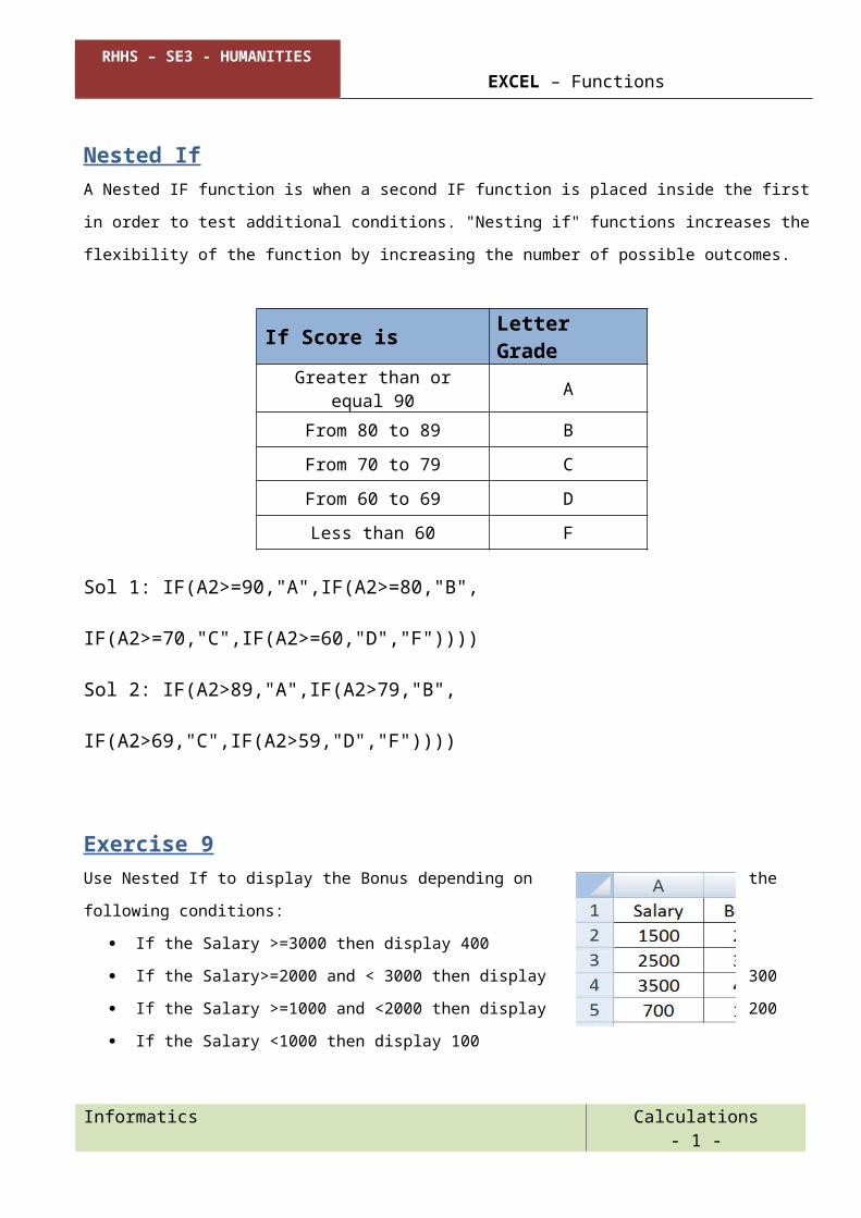
Exercise 9 Use Nested If to display the Bonus depending on the following conditions:

If the Salary >=3000 then display 400 If the Salary>=2000 and < 3000 then display 300 If the Salary >=1000 and <2000 then display 200 If the Salary <1000 then display 100

If(a2>=3000,”400”,if(a2>=2000,”300”,if(a2>=1000,”200”,”100)))

Informatics Calculations - 1 -


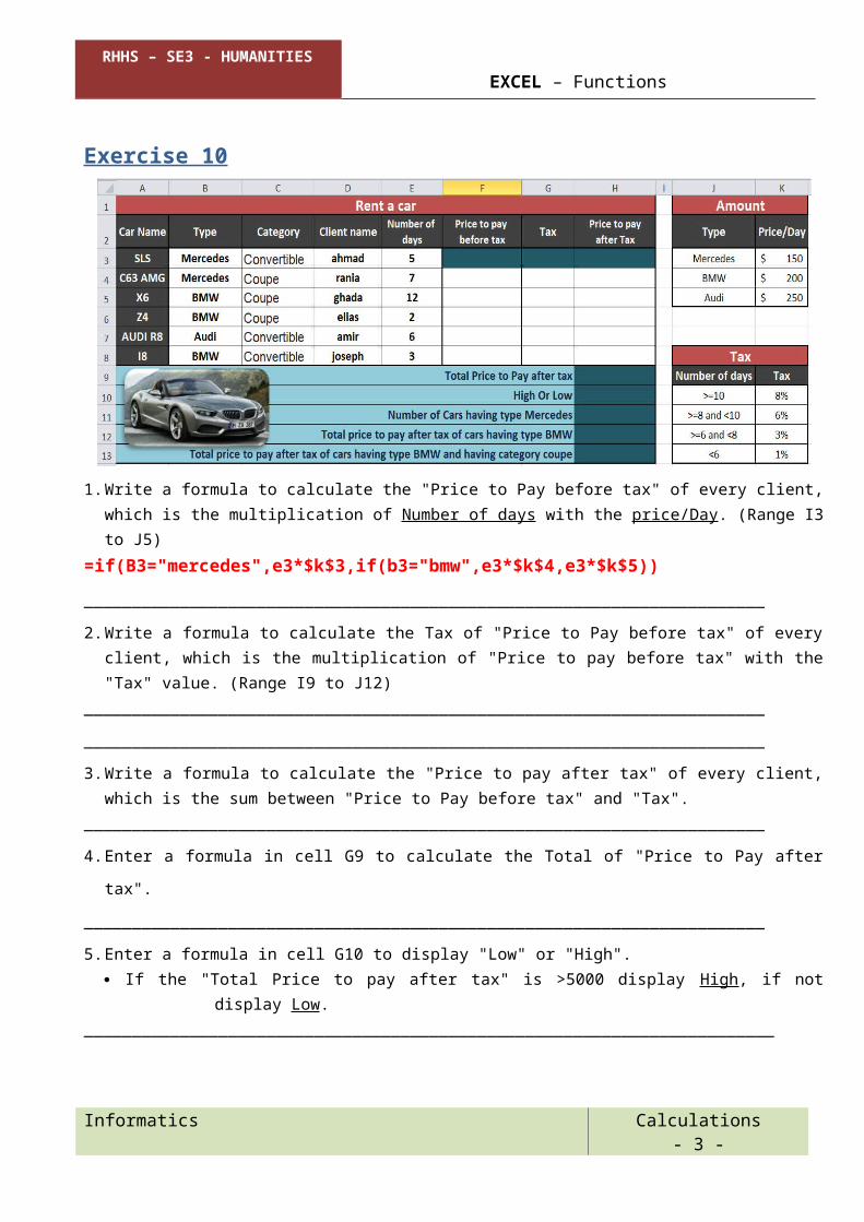
Exercise 10

1. Write a formula to calculate the "Price to Pay before tax" of every client, which is the multiplication of Number of days with the price/Day. (Range I3 to J5)

=if(B3="mercedes",e3*$k$3,if(b3="bmw",e3*$k$4,e3*$k$5))_______________________________________________________________________2. Write a formula to calculate the Tax of "Price to Pay before tax" of every client, which is

the multiplication of "Price to pay before tax" with the "Tax" value. (Range I9 to J12)______________________________________________________________________________________________________________________________________________3. Write a formula to calculate the "Price to pay after tax" of every client, which is the sum

between "Price to Pay before tax" and "Tax"._______________________________________________________________________4. Enter a formula in cell G9 to calculate the Total of "Price to Pay after tax"._______________________________________________________________________5. Enter a formula in cell G10 to display "Low" or "High".

If the "Total Price to pay after tax" is >5000 display High, if not display Low.________________________________________________________________________



And Operator

"AND" will return True ONLY if all the value entered evaluate to True. If only one from many conditions, evaluate to False and the rest are True, the AND Function will return False.

Syntax: =IF (And(Condition1,Condition2),Value-True, Value-False)

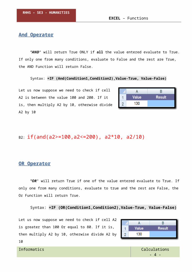
Let us now suppose we need to check if cell A2 is between the value 100 and 200. If it is, then multiply A2 by 10, otherwise divide A2 by 10

B2: if(and(a2>=100,a2<=200), a2*10, a2/10)

OR Operator

"OR" will return True if one of the value entered evaluate to True. If only one from many conditions, evaluate to true and the rest are False, the Or Function will return True.

Syntax: =IF (OR(Condition1,Condition2),Value-True, Value-False)

Let us now suppose we need to check if cell A2 is greater than 100 Or equal to 80. If it is, then multiply A2 by 10, otherwise divide A2 by 10

B2: if(OR(a2>=100,a2=80), a2*10, a2/10)



Exercise 11

Calculate the augmentations

Augmentation 1 is 12% of the salary for all employees having experience year more than 10 years.

=IF(C2>10,D2*12/100,0)

Augmentation 2 is 14% of the salary for employees having department accounting or informatics, and 16% of employees having department marketing, and 18 % for other department.

IF(OR(B2="ACCOUNTING",B2="INFORMATICS"), D2*14/100, IF(B2=”MARKETING”, D2*16/100, D2*18/100))

Augmentation 3 is 10% of the salary for employees having salary >= 1000000 and <=2000000, and 12% of the other employees.

=IF(AND(D2>=1000000,D2<=2000000),D2*10/100,D2*12/100))

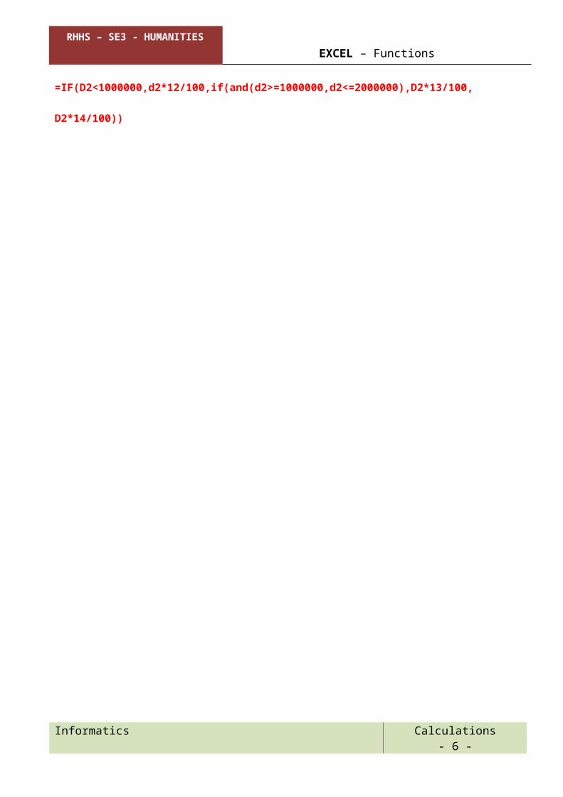
Augmentation 4 is 12% of the salary for employees having salary <1000000 and 13% for employees having salary between 1000000 and 2000000, and 14% for employees having salary >=2000000.

=IF(D2<1000000,d2*12/100,if(and(d2>=1000000,d2<=2000000),D2*13/100,

D2*14/100))



3-D Cell Reference To consolidate data from several worksheets into a single worksheet, you have to

use the 3 – D reference formulas.By using the 3 –D reference formulas, data and formulas can be shared among different worksheets in the same workbook. If you change the numeric data in the worksheet that your formula refers to, the result of the formula will be automatically updated according to the new values.

Example: =(Midyear!A5 + Final!A5)/2

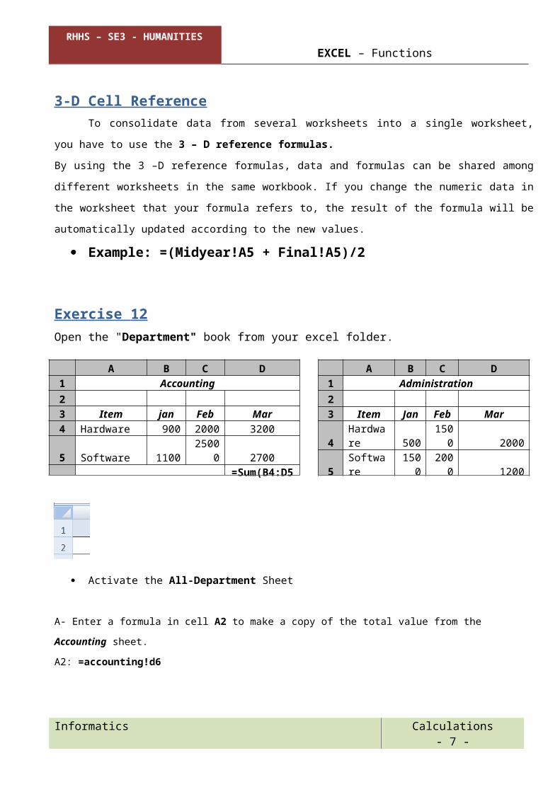
Exercise 12 Open the "Department" book from your excel folder.

Activate the All-Department Sheet

A- Enter a formula in cell A2 to make a copy of the total value from the Accounting sheet.A2: =accounting!d6

B- Enter a formula in cell B2 to make a copy of the total value from the Administrationsheet. B2: =administration!d6

C- Enter a formula in cell C2 to calculate the Total, which is the Sum of the payments for the two departments. C2=a2+b2


A B C D1 Administration23 Item Jan Feb Mar

4Hardware 500

1500 2000

5 Software150

0200

0 1200=Sum(B4:D

A B C D1 Accounting23 Item jan Feb Mar4 Hardware 900 2000 3200

5 Software 11002500

0 2700

6 Total=Sum(B4:D5

)


VLOOKUP VLOOKUP is an Excel function to lookup and retrieve data from a specific column in table. "V" stands for "vertical".

Lookup values must appear in the first column of the table, with lookup columns to the right

Syntax =VLOOKUP (lookup_value, table_array, Col_index_num, range_lookup)

Lookup_value: The value to be found in the first column of the table. Table_array A table of information in which data is looked up. Col_index_num The Column number in table_array from which the matching

value will be returned. Range_lookup A logical value that specifies whether you want VLOOKUP to find

an exact match or an approximate match. Use the word TRUE for an approximate matching value to be returned and use the word FALSE, to find an exact matching value to be returned.

Example 1: Exact match

In most cases, you'll probably want to use VLOOKUP in exact match mode.

This makes sense when you have a unique key to use as a lookup value, for example, the ID in this data.

Example 2: Approximate match

Sometimes, you want to use an approximate mode in cases when you're looking for the best match, not an exact match. A classic example is finding the right commission rate based on a monthly sales number. In this example, the formula in D5 performs an approximate match to retrieve the correct commission.



Exercise 13

The name of the following sheet is Emp-Bonus

In cell B2, write the formula to get the name of the employee depending on their ID.=VLOOKUP(B1,A9:D11,2,FALSE)

In cell B3, write the formula to get the number of children of the employee depending on their ID.=VLOOKUP(B1,A9:D11,3,FALSE)

In cell B4, write the formula to get the salary of the employee depending on their ID.=VLOOKUP(B1,A9:D11,4,FALSE)

In cell B5, write the formula to get the bonus of the employee depending on their number of children (exists in the sheet Emp-Bonus).________________________________________________________________________In cell B6, write the formula to calculate the new salary (salary + bonus).__________________________________________________________________



Text Function

The TEXT function converts a numeric value to text and lets you specify the display formatting by using special format.

Syntax

TEXT(value, format_text)

The format "dddd" is used to display the day of the date.

The format "mmmm" is used to display the month of the date.

The format "yyyy" is used to display the year of the date.

Example: the function =TEXT(1/2/2017,"dddd") displays Saturday.


Documents

pROGRAMMING lANGUAGE - se3 …se3-informatics.wikispaces.com/file/view/1- SE3 - Excel - Quiz 2... · Web viewWrite a formula to calculate the Tax of "Price to Pay before tax" of every