RESIDENTIAL VERTICAL GEOTHERMAL HEAT PUMP SYSTEM MODELS: CALIBRATION TO DATA J.W. Thornton T.P. McDowell J. Shonder P.J. Hughes D. Pahud G. Hellstrom ASHRAE Member ASHRAE Member ASHRAE Member ABSTRACT A detailed component-based simulation model of a geothermal heat pump system has been calibrated to monitored data taken from a family housing unit located at Fort Polk, Louisiana. The simulation model represents the housing unit, geothermal heat pump, ground heat exchanger, thermostat, blower and ground loop pump. Each of these component models were "tuned" to better match the measured data from the site. These tuned models were then interconnected to form the system model. The system model was then exercised in order to demonstrate its capabilities. KEY WORDS Geothermal, heat pump, Ft. Polk, calibration, modeling, simulation, GHP, ground source, energy savings performance contract, ESPC, ground heat exchanger, DST.

RESIDENTIAL VERTICAL GEOTHERMAL HEAT PUMP SYSTEM MODELS: CALIBRATION TO DATA ABSTRACT A detailed component-based simulation model of a geothermal heat pump system has been calibrated to monitored data taken from a family housing unit located at Fort Polk, Louisiana. The simulation model represents the housing unit, geothermal heat pump, ground heat exchanger, thermostat, blower and ground loop pump. Each of these component models were "tuned" to better match the measured data from the site. These tuned models were then interconnected to form the system model. The system model was then exercised in order to demonstrate its capabilities. INTRODUCTION With the implementation of a large-scale energy savings performance contract (ESPC) at Ft. Polk, Louisiana, the heating and cooling systems in each of the military base's 4003 family housing units was retrofitted with a geothermal (ground source) heat pump (GHP). Each of the GHP's at Ft. Polk feature multiple vertical U-tube ground heat exchangers plumbed in parallel to reject/absorb energy to/from the earth. Independently of the ESPC, an evaluation was conducted to verify the energy and demand savings and explore means of improving the economics of future projects. This evaluation included field data collection at the electric feeder level (total power consumption by all apartments served by the feeder), the apartment level (total power consumption of the building), the end-use level, and the “energy balance (technology assessment)” level (sufficient data collection (temperature, flow rate, power, run-time, etc.) to perform an accurate energy balance around each piece of installed equipment). This detailed "energy balance" monitoring was performed on 5 of the 4003 housing units; a representative 5-plex apartment building. A component-based simulation model of one of the “energy balance” monitored housing units has been calibrated against the field data. This "tuned" simulation model can then be used to predict the performance of the GHP systems with various design changes; offering valuable insight on how design changes might impact performance and operating conditions. GROUND SOURCE HEAT PUMP CONFIGURATION Of the 5 "energy balance" monitoring sites at Ft. Polk, one housing unit was chosen for the simulation model calibration documented here. The unit selected had the longest post-retrofit data set while being occupied for the duration of the monitoring period. The unit selected is one of the lower apartments in the two-story building. This unit has a conditioned floor area of 1052 square feet (98 m2) and is equipped with a GHP with the following characteristics: nominal 1.5 ton (17300 btuh) total cooling capacity and 15.4 EER at ARI 330 rating conditions, and an 11800 btuh heating capacity and 3.5 COP at ARI 330 rating conditions. This GHP used water as the ground loop working fluid and came equipped with a desuperheater for supplying domestic hot water. Two vertical U-tube ground heat exchangers connected in a parallel

arrangement were used to reject/absorb heat to/from the earth. Each of the vertical U-tube ground heat exchangers was placed in a vertical borehole of 4.125 inch (0.10477 m) diameter and 258 foot (78.64 m) depth. These boreholes were spaced 16 feet (4.88 m) apart, 25 feet (7.62 m) from the exterior wall and were backfilled with a bentonite-based grout after the installation of the U-tubes. The U-tubes themselves are comprised of 1 inch nominal (0.0254 m) SDR-11 polyethylene pipe (1.08 inch ID, 1.31 inch OD) with a nominal center-to-center spacing of 2.565 inches (0.065 m). The center-to-center U-tube spacing exists at the bottom of the U-tube heat exchanger (the bottom of the bore). No extraordinary measures were taken to maintain this spacing along the length of the bore. The horizontal runouts to the boreholes, and the horizontal piping between the bores, are buried at a depth of 3 feet (0.914 m) with outbound and return legs in separate trenches. Refer to Figure 1 for a graphical representation of the ground heat exchanger configuration.

ENERGY BALANCE MONITORING The detailed "energy-balance" monitoring began in late 1995 and continued through February of 1997. The following points were measured and recorded as 15-minute averages or totals: • Whole Premise Power • GHP Entering Water Temperature (when on) • Total GHP Power • Ground Heat Exchanger Temp. Difference • GHP Compressor Power • Desuperheater Pump Status • Water Heater Power • Desuperheater Inlet Temperature (when on) • Blower Status • Desuperheater Temperature Difference (when on) • Ground Loop Pump Status • Reversing Valve Status • Ambient Temperature • Ambient Relative Humidity In addition to the 15-minute data, one-time measurements of several key parameters were also recorded. These included blower power draw, loop pump power draw, desuperheater pump power draw, ground loop flow rate, and desuperheater flow rate. It was argued that desuperheater operation might confound some of the calibration steps. For this reason for most of the recording period the desuperheater was intentionally disabled. The calibrations reported here are for periods where the desuperheater was not operational. DETAILED SIMULATION MODEL The public domain TRNSYS (Klein, 1996) simulation software package was chosen as the platform for the detailed models because it can operate at any timestep (so ground heat exchanger models requiring small timesteps to be stable and accurate could be used) and it is relatively easy to drive with measured data. TRNSYS is a modular system simulation package where the user describes the components that comprise the system and the manner in which these components are interconnected. Components may be pieces of equipment such as a pump or thermostat or utility modules like occupancy forcing functions, weather data readers, integrators and printers. Because the program is modular, new component models for the heat pump and vertical ground heat exchanger were easily added to the existing component libraries to expand the capabilities of the program to include residential GHP systems.

Unlike most of the commonly used building energy analysis tools, TRNSYS can operate in either "temperature-level" or "energy-rate" control (Klein, 1996). In "energy-rate" control, the heating/cooling loads are calculated based only upon the net heat losses/gains from the conditioned space. The user specifies the set point temperatures for heating and cooling. The program then calculates the amount of energy required to keep the conditioned space at these set points. The calculated loads are then passed to the conditioning equipment; which exactly meets these loads at every timestep. The advantage in using energy rate control is that the loads for a given structure can be calculated once and then re-used in subsequent equipment and plant simulations. However, the detailed interaction between the conditioned space and the equipment is not treated directly. In "temperature-level" control, the temperature of the conditioned space is a function of the ambient conditions as well as the inputs of the equipment. In this mode, a controller is required to command the equipment. For these reasons, "temperature-level" control results in a more realistic and detailed simulation of the interaction between the conditioned space and the equipment. The equipment is either on or off each timestep and delivers whatever capacity would be expected given the operating conditions at that time. An earlier study (Hughes, 1980), has demonstrated the value of using "temperature-level" control as opposed to "energy-rate" control in heat pump system studies. The software performs the dynamic transient analysis at user-defined timesteps, iterating at each timestep until the system of equations created by the interconnection of the component model inputs and outputs is solved. For this work, a timestep of 15 minutes was chosen after considering accuracy, stability requirements, typical equipment cycle times, recorded data intervals, and simulation speed. In order to characterize the performance of the system, the performance of each of the components which comprise the system must be characterized. In this case, the system components were chosen to be the building and its associated forcing functions, the heat pump, the ground heat exchangers, the thermostat, the ground loop pump, and the heat pump blower. The operation of each of these components will be briefly described below. For reference, a TRNSYS assembly panel schematic of the system information flow is included as Figure 2.

Weather: Although the ambient temperature and relative humidity were measured at the site, these values were not used in simulations using the detailed heating/cooling load model due to the lack of solar radiation measurements. (Note: as explained later, the measured temperature and relative humidity data were used in simulations using a simplified load model that can be driven with just these inputs). Instead, Typical Meteorological Year (TMY) weather from Lufkin, TX was used for the simulations, as Lufkin represents the closest inland TMY site to Ft. Polk. An earlier study had shown slight differences in the long-term averages for Lufkin, TX and Alexandria, LA, the closest location to Ft. Polk with published bin data (Right-Loop, 1992). The TMY weather, which is a monthly best-fit average of 30-years of weather data, contains ambient temperature, relative humidity, incident solar radiation, and wind speed values at hourly increments for a year. When the timestep for the simulation is less than the weather data interval, as was the case here, TRNSYS interpolates the weather data. The incident solar radiation on each of the exterior surfaces was processed and subject to overhang and wingwall shading effects as the chosen housing unit has many such features. For reference, the design temperatures (1% value) for Ft. Polk, LA are (ASHRAE, 1989):

• Winter Design Temperature = 23 F (-5 C) • Summer Design Temperature = 95 F (35 C) • Daily Temperature Range = 20 F (11.1 C)

A new TRNSYS component based on the Kusuda correlation (Kusuda, 1965), was developed to estimate the ground temperature for the simulation . This new model takes as input, the average surface temperature, the amplitude of the surface temperature, and the phase delay and calculates the hourly distribution of ground temperature with depth. For reference, the published values of these properties (ASHRAE, 1977) for Alexandria, LA are:

• Mean soil surface temperature = 69 F (20.6 C) • Amplitude of surface temperature = 17 F (9.4 C) • Day of minimum surface temperature = 32

Building Load Model: The detailed heating and cooling load model chosen for this simulation was the standard multi-zone building load model in TRNSYS. This model implements a non-geometrical balance model with one air node per zone. The model accounts for the effects of both short-wave and long-wave radiation exchange, internal generation (both sensible and latent), occupancy effects, infiltration effects, ventilation effects, and convective exchanges. The walls, ceilings, and floors are modeled according to the ASHRAE transfer function approach (ASHRAE, 1977). For this work, the building model was assumed to have one thermal zone representing the conditioned volume of the chosen unit. An earlier analysis by the authors had shown negligible energy differences when compared against the same unit modeled with 10 thermal zones; 7 conditioned zones (kitchen/dining, family room, two bedrooms, bathroom, hallway, and utility room) and 3 unconditioned zones (3 storage areas). The interactions between this zone and the apartments next door and upstairs, the ambient, and the ground (slab floor) were also considered. For this study, the internal gains to the space from lighting, equipment, and occupancy were scheduled based on the time of day. The daily differences (weekend effects) were not considered. The infiltration to the zone was modeled based on a modified ASHRAE method (ASHRAE, 1977) that calculates the air changes per hour based on the wind speed and the temperature difference between ambient and conditioned space. As explained above, when operated in “temperature level control”, the TRNSYS software is somewhat unique in that the thermal interaction between the zone and the conditioning equipment is dynamic. This is unlike other tools that calculate the building loads and pass these loads to the equipment/plant models. In TRNSYS, the zone temperature is a function of the equipment response (on/off, capacity if on, etc.), which is a function of the zone temperature. Thermostats: The standard TRNSYS thermostat model was used for this work. The thermostat model accounts for hysteresis effects. When the temperature of the zone rises above the temperature set point for cooling (or falls below the temperature setpoint for heating) the thermostat calls for cooling (or heating) and continues to call for cooling (or heating) until the temperature of the zone falls below the cooling setpoint temperature minus a user-specified dead-band temperature (or rises above the

heating temperature setpoint plus a user-specified dead-band temperature). The thermostat setpoints did not take into account night setback/setup, although this is possible, because the equipment at Ft. Polk is not operated in that manner. Ground Loop Pump: The ground loop pump used for this study was a simple constant flow pump model. When the thermostat calls for conditioning, the pump flows a steady value of 4.64 gallons per minute (0.293 l/s); the one time measurement from the site. Start-up and shut-down power and flow transients are neglected as is the effect of varying pressure drop due to water property changes with temperature. The power consumed by the ground loop pump is assumed constant; calculated as described in later sections. The model also allows for a fraction of the loop pump power to be converted to flow energy. For this study, all the ground loop pump power was assumed to be converted to flow energy (i.e., dissipated as heat into the fluid rather than radiated from the pump housing). In this way, calculations to determine the required ground heat exchanger length will be slightly conservative when cooling is the dominant factor in determining the ground heat exchanger length (as is the case at Ft. Polk). The pump model assumes that the power instantaneously reaches its steady-state value at the beginning of an on-cycle and instantaneously drops to zero at the end of an on-cycle. Blower: Like the ground loop pump, the blower used for this study was a simple constant flow device. When the thermostat calls for conditioning, the blower moves 600 cubic feet per minute (0.283 m3/s) of air across the heat pump coil; the nominal value from the catalog of performance data for this heat pump. This value was used since reliable measurements of air flow rates were not available. Start-up and shut-down power and flow transients were neglected as was the effect of varying pressure drop due to air property changes with temperature and humidity. The power consumed by the blower was a constant; calculated as described in later sections. The model also allows for a fraction of the blower power to be converted to flow energy. For this study, all the blower power was assumed to be converted to energy used to increase the temperature of the air stream. The blower model assumes that the power instantaneously reaches its steady-state value at the beginning of an on-cycle and instantaneously drops to zero at the end of an on-cycle. Heat Pump: A new water source heat pump model was written for TRNSYS for this project. The heat pump model uses a look-up table approach in both heating and cooling mode to determine the manufacturer's published catalog data for capacity, power, and water heat transfer. Inputs to the model include the entering water temperature and flow rate, the entering air temperature, humidity ratio, and flow rate, and the control signal from the thermostat. Outputs from the model include the calculated values of leaving water temperature and flow rate, exiting air temperature, humidity ratio, and flow rate, and the equipment capacity and power draw. The first table is entered with the input value of water flow rate in gallons per minute (gpm) and the input value of entering water temperature. In heating mode, the steady-state heating capacity, the steady-state heat pump power (blower+controls+compressor), and the steady-state heat absorption rate from the water are interpolated from the data set. In cooling mode, the total steady-state cooling capacity, the sensible steady-state cooling capacity, the steady-state heat pump power (blower+controls+compressor), and the steady-state heat rejection rate to the water are interpolated from the data set.

The second table is entered with the known air flow rate (cfm) to obtain the published correction factors for steady-state capacity, steady-state power, and the steady-state heat rejection/absorption. The final table is entered with the entering air dry bulb temperature (heating mode) or the air dry and wet bulb temperatures (cooling mode) to determine the published correction factors. In cooling mode, the correction factors for steady-state capacity (both total and sensible), and the correction factors for steady-state heat rejection to the water are read from the table. In heating mode, the correction factors for steady-state heating capacity, steady-state heat of absorption from the water, and steady-state power are read from the table. In order to allow for typical discrepancies between published catalog capacities and measured capacities, the heat pump model scales the calculated steady-state capacity values by a user-defined fraction. The heat pump model assumes that the heat pump power draw instantaneously reaches its steady-state value at the beginning of an on-cycle and instantaneously drops to zero at the end of an on-cycle. The model also assumes that the capacity ramps up asymptotically at the start of an on-cycle and drops to zero instantly at the end of an on-cycle. The time constant of the capacity ramp is user input. Energy balance and psychrometric calculations at each iteration assure that the results from the model at each timestep are reasonable.

Ground Heat Exchangers: For GHP systems, the most important component model is the ground heat exchanger. Although several ground heat exchanger models were available for this study, the duct ground heat storage model (DST) was chosen for this study because it is well documented, validated, and considers multi-bore interactions and long-term (multi-year) effects. The duct ground heat storage model (DST) was developed at Lund University (Sweden) and chosen in 1981 by the participants of the International Energy Agency, Solar R&D Task VII (Central Solar Heating Plant with Seasonal Storage) for the simulation of duct ground heat storage. A simpler but faster version was implemented by Hellstrom (1983) in the MINSUN program (Mazzarella, 1991), a simulation tool for the optimization of a central solar heating plant with a seasonal storage (CSHPSS). A TRNSYS version based on this faster DST version was implemented by Mazzarella in 1993. A more recent version (Hellstrom et al., 1996) combined the easy utilization of the simple version with the additional features of the more detailed original DST program (Hellstrom, 1989). In addition, a detailed computation of the local heat transfer along the flow path within the storage region was also possible (Pahud and Hellstrom, 1996). The latest version (Pahud et al., 1996) offers the possibility of having several ground layers that cross the storage region, each having their own thermal properties. In DST, a duct ground heat storage system is defined as a system where heat or cold is stored directly in the ground. A ground heat exchanger, formed by a duct (borehole) or channel system, is used for heat exchange between a heat carrier fluid, which is circulated through the boreholes, and the storage region. The heat transfer from the borehole system to the surrounding ground is approximated by pure conduction. The DST model is a simulation model for characterizing such ground heat storage systems. The storage volume (the volume of earth containing the boreholes) has the shape of a cylinder with a vertical symmetry axis. The boreholes are assumed to be uniformly placed within this storage

volume. There is convective heat transfer in the boreholes and conductive heat transfer in the ground. It is convenient to treat the thermal process in the ground as a superposition of a global and a local problem. The global problem handles the large-scale heat flows in the storage and the surrounding ground, whereas the local problem takes into account the heat transfer between the heat carrier fluid and the storage. The local problem uses local solutions around the boreholes and a steady-flux part, by which the number of local solutions, and thereby computation time, can be reduced without significant loss of accuracy. The global and the local problems are solved with the use of the explicit finite difference method (FDM), whereas the steady-flux part is given by an analytical solution. The total temperature at one point is obtained by a superposition of these three solutions. The short-time effects of the injection/extraction through the boreholes are simulated with the local solutions, which depend only on a radial coordinate and cover a cylindrical volume exclusively ascribed to each borehole. As the model assumes a relatively large number of boreholes, most of the boreholes are surrounded by other boreholes. In consequence, a zero heat flux at the outer boundary is prescribed, due to the symmetrical positions of the neighboring boreholes. This assumption may lead to the under-prediction of heat transfer to the ground in cooling mode for installations with only a few boreholes. The heat transfer from the fluid to the ground in the immediate vicinity of the borehole is calculated with a heat transfer resistance. A steady-state heat balance (performed each time step) for the heat carrier fluid gives the temperature variation along the flow path. The local solution may take into account a radial stratification of the storage temperatures (due to a coupling in series of the boreholes), as well as increased resolution in the vertical direction. The local heat transfer resistance from the fluid to the ground (or borehole thermal resistance) may depend on the flow conditions, i. e., it can be temperature and flow dependent. It may also take into account the unfavorable internal heat transfer between the downward and upward legs of the U-tube in a borehole. The three-dimensional heat flow in the ground is simulated using a two-dimensional mesh with a radial and vertical coordinate. The model assumes homogeneous and constant thermal properties within a horizontal ground layer. Several ground layers are permitted and the thermal properties may vary from layer to layer. Insulation may be placed on the top and sides of the storage volume. A time-varying temperature is given for the ground surface.

CALIBRATING THE SIMULATION MODEL Although a detailed simulation model of the thermal system at the chosen unit provides a very useful tool in developing trends and evaluating the system operation, the same model calibrated to measured site data greatly increases the confidence in the answers that the simulation provides. Due to its modular nature, tuning the system in TRNSYS implies tuning each of the individual component models. The process used to tune each of the important system components is described briefly below.

Controllers: Even with the heat pump compressor and blower motor off, there is power draw by the packaged heat pump unit. This power draw can be attributed to the heat pump controls. To quantify this power draw, the intervals in the data where the heat pump compressor, blower, and loop pump were off for the entire 15-minute interval were stripped from the data. When plotted for the year, the control power is seen to be very different in heating and cooling modes. This difference is thought to be due to the reversing valve for the heat pump. Figure 3 shows these differences for the month of April; the only month with both heating and cooling cycles. Also plotted on Figure 3 is the position of the reversing valve (0=heating, 1 = cooling). For simulation purposes, a controller power draw of 6 Watts was assumed for heating mode and a value of 20 Watts was assumed for cooling mode. These values represent the averages over the heating and cooling seasons respectively. This controller power draw, along with the blower power draw, will be subtracted from the calculated heat pump power (read from the catalog data at each timestep) to determine the heat pump compressor power. Blower: During a portion of the monitoring period for this work, special controls were in place that removed direct compressor control from the occupants. Changing the thermostat setting only affected the operation of the blower. Compressor operation was driven by a return air temperature sensor. This knowledge was then used to tune the blower model. The 15-minute periods where the blower was on, but the compressor and ground loop pump were off were stripped from the data set. During these periods, the measured power consumption of the packaged heat pump unit is equal to the power consumption of the blower motor plus the controller power. The blower power can then be estimated as the power consumption in the 15-minute recording period minus the assumed controller power divided by the blower run time. When plotted for the calibration period, the blower power draw is seen to decay from a value of ~160 Watts in February to a value of ~130 Watts in April. The blower power draw could not be checked after April due to the return to standard compressor controls. The one-time site measurement, taken early in the year, of 160 Watts compares well to the early calculations. The decay in blower power draw was thought to be caused by an increasingly dirty air filter. Although the one-time site measurement of blower power (160 W) was verified for the early part of the year, a calibration value of 130 Watts was selected as a better representation of actual operation. To investigate whether there were start-up "spikes" in blower power, the intervals where just the blower was on, and had just turned on, were stripped from the data. Plots of these values indicate that the average value at start-up is indistinguishable from the calculated steady-state value. The blower model's assumption that the power instantaneously reaches its steady-state value of 130 Watts at turn-on and remains at that value until turn-off (in which case it immediately drops to zero) appear valid. Reliable one-time measurements of air flow rate in cubic feet per minute were not available. The value of 600 cfm (0.0283 m3/s) was used for the calibration. The manufacturer's catalog data reveals that a 15% change in air flow rate results in only a 1% change in total capacity, water heat transfer, and power consumption. The air flow rate was therefore assumed to reach its steady-state value instantaneously at blower turn-on and remain at that value until turn-off (in which case it immediately drops to zero).

Thermostat: With the original controls, the occupants had no direct control over the heating and cooling setpoints. The thermostats only controlled the operation of the blower; a return air thermostat controlled the operation of the heat pump compressor. However, many of the tenants of these housing units had found ways of fooling the systems (heat lamps on the return air sensor for example) and were causing maintenance problems. For these and other reasons, the system was converted to standard compressor controls (thermostat cycles compressor) in April. In an attempt to resolve what the heating and cooling setpoints were for the year, the indoor temperature at the initiation and termination of heating and cooling periods was stripped from the data and plotted for each month. The thermostat setpoints and dead bands were extremely important in determining the building energy loads and the heat pump cycle times (which affect the maximum heat pump entering water temperature predictions). As feared, the results (shown in Table 1) showed varying thermostat setpoints in each month.

Figures 4 and 5 show the turn-on and turn-off temperatures for cooling in the months of May and August. Notice the discernible deadband temperature difference (the temperature difference between turn-on and turn-off) in the month of May and the general lack of a dead-band temperature difference in August. This lack of a discernible temperature difference between turn-on and turn-off is due to the heat pump turning on and off in each of the 15-minute intervals in the month of August. With no distinct heating and cooling setpoints available from the data set, the thermostat model in TRNSYS was modified to accept unique monthly values of the heating and cooling setpoints and the thermostat deadbands. Because there are times of the year at which the cooling set point temperature is below the heating set point temperature, heating and cooling seasons were established for the model. As taken from the data set (which records the position of the reversing valve), the heating season runs from October 3rd until April 13th. Ground Loop Pump: To verify the one time field measurement of the power draw for the loop pump, the data intervals when there was heat pump operation for the entire 15-minute interval were stripped from the data. During these intervals, the electric consumption of the loop pump is equal to the packaged heat pump consumption minus the consumption of the compressor, the blower, and the controls. The electric consumption of the packaged heat pump and the compressor were recorded in the data and the blower and controller consumption were estimated as discussed above. The calculated electric consumption of the loop pump was then divided by the heat pump run time to determine the power draw of the loop pump. The one-time site measurement of loop pump power (220 W) was then used for the calibrated value as plots of measured loop pump power confirm this recorded value. The assumption was also made that the power instantaneously reaches its steady-state value at turn-on and remains at that value until turn-off (in which case it immediately drops to zero). The ground loop pump flow rate is one of the critical parameters for the simulation as both the heat pump and ground heat exchanger performance depend on this value. Without a means of determining the ground loop flow rate from the monitored data set, the measurement of loop pump flow rate at the site was assumed to be the steady-state value for the calibration.

Ground Heat Exchanger: The calibration of the detailed ground heat exchanger model was intended to be relatively straightforward. Where possible, known values of the ground heat exchanger parameters were used. These values included the known heat exchanger geometric data (borehole diameter and depth, header depth, borehole spacing, U-tube pipe sizes and shank spacing), and the thermal properties of the polyethylene pipe and the grout (backfill) material (thermal conductivity, density, and specific heat). The detailed simulation did not include the piping runouts to the ground heat exchangers nor the horizontal buried pipes between the ground heat exchangers. The remaining parameters, deep earth temperature and the soil thermal properties (thermal conductivity, density, and specific heat), were varied to try and achieve a "best fit" soil. This "best fit" effective soil also lumps together any vertical variations in soil properties plus the impact of the horizontal runouts and the horizontal buried pipe between the ground heat exchangers. The "best fit" soil is that soil which best matches the 15-minute recorded data for heat pump entering water temperature versus the model predictions for heat pump entering water temperature. The goal of this study was not to try and demonstrate how accurate the ground heat exchanger model predictions can be when the soil thermal property assumptions are "best-fit" to data (as this "best-fit" process tends to mask any errors or poor assumptions in the ground heat exchanger model), but rather to develop an accurate prediction of the performance of this ground heat exchanger over a range of operating conditions. This "tuned" heat exchanger model can then be expected to provide reasonably accurate simulation results when coupled with other calibrated models. With an accurate estimate of the heat pump leaving water temperature (which is the ground heat exchanger inlet temperature), this process would have been simple. However, after much investigation it was determined that the temperature difference sensor used to calculate the heat pump leaving water temperature was inaccurate at the flow rates at which the heat pump was operating. This was true for all 5 of the "energy-balance" monitoring sites. Without the heat pump leaving water temperature, it was impossible to calculate the amount of energy that was absorbed from/rejected to the soil. The only possible path around this obstacle was to estimate the amount of energy transfer to/from the soil by using the manufacturer's catalog data. This estimation was left to the heat pump component model which allowed for a user-defined fraction of the catalog steady-state capacity to be used. For the purposes of this work, 95% of the published catalog heating and cooling capacities were used for the steady-state heat pump capacities. The model also assumes that the capacity ramps up asymptotically at the start of an on-cycle and drops to zero instantly at the end of an on-cycle. The time constant calculation is described in the heat pump calibration section. The measured loop-temperature data from the site was recorded in 15-minute averages with loop pump run-times also recorded for the 15-minute period. The TRNSYS program operates in discrete timesteps; the heat pump is either on or off for the timestep, not on for a fraction of the timestep. It was therefore necessary to run TRNSYS on a sub 15-minute timestep. A timestep of 1 minute was chosen for the soil calibration. The 15-minute recorded data had to then be discretized into 1 minute segments. The first step in determining 1 minute data from 15 minute averages was to arrange the equipment runtimes in a logical sequence. There are six different scenarios for the operation of the heat pump during a 15 minute interval ranging from the heat pump operating for the whole fifteen minutes period to the heat pump being off for the whole fifteen minute period. The 15-minute data was discretized into 1-minute segments by arranging the run-times based on the

state of the heat pump at the current, previous and next 15-minute periods. This form of discretization was done to try and match the actual cycling times as well as possible. During each 1-minute timestep, the heat pump leaving water temperature is calculated based on the measured 15-minute average heat pump entering water temperature and the heat pump's calculated heat rejection/absorption; which is a function of the heat pump entering water temperature and time. This heat pump leaving water temperature, the one-time measurement of the flow rate, and the measured ambient conditions drive the ground heat exchanger model to produce a "predicted" heat pump entering water temperature. With these inputs from the monitored data and the heat pump model, and with the ground properties of thermal conductivity, the product of specific heat and density, and deep earth temperature varied as parameters, the "predicted" temperature from the ground heat exchanger model in TRNSYS was compared to the outlet temperature from the ground heat exchanger (entering heat pump water temperature) from the collected data to determine "best fit" properties for the soil. Since the collected data was originally in fifteen minute averages, the TRNSYS output was compiled into fifteen minute averages for comparison. The simple statistical comparison to determine "best fit" was done by taking the difference between the "predicted" values and the collected data for each fifteen minute interval when the heat pump operated for the entire interval and squaring this value. These squares of the difference were summed over the length of the simulation and the soil properties with the lowest value were selected as the "best fit" values. The results of the "best match" of the soil properties for this unit correspond almost exactly to the ASHRAE heavy saturated soil; a density of 200 lbm/ft3 (3200 kg/m3), a specific heat of 0.20 BTU/lbm.R (0.84 kJ/kg.K), and a thermal conductivity of 1.40 BTU/h.ft.R (8.722 kJ/h.m.K). The corresponding deep earth temperature was found to be approximately 62 degrees Fahrenheit (16.67 C). The ground heat exchanger calibration was performed for the month of May; a month in which the heat pump only ran in cooling mode. With the known borehole geometry and the "best-fit" soil properties, a pipe-to-soil thermal resistance of 0.2281 hr.ft.F/BTU (0.1318 m.K/W) was calculated by the DST model. With these effective soil properties, an average temperature difference between measured and predicted values when the heat pump was operating of 0.145 degrees Fahrenheit (0.081 C) was observed over the month long test period. Figure 6 shows the "predicted" and measured 15-minute averages for three days near the end of the soil calibration test. These "reverse-engineered" soil properties contradict an earlier independent analysis (before the GHP installations) of the soil (Ewbanks, 1995) at three locations around the base. The results from the earlier analysis are shown below (the housing unit used for this study is located in the South Fort area):

South Fort: Soil Type = Sand, Thermal Conductivity = 1.156 BTU/hr.ft.F (2.001 W/m.K) Mid Fort: Soil Type = Clay, Deep Earth Temperature = 67.8 F (19.89 C) Thermal Conductivity = 0.802 BTU/hr.ft.F (1.388 W/m.K)

North Fort: Soil Type = Clay/Sand, Thermal Conductivity = 0.964 BTU/hr.ft.F (1.668 W/m.K)

The earlier independent analysis was based on six-hour data sets where a thermal test unit was used to heat and pump approximately 6 gpm (0.378 l/s) of water through a ground heat exchanger similar to the one installed at the site. The supply and return temperatures were measured and the soil thermal conductivity calculated for the test site. The property calibration presented here is based on all cycles of an operating system for the period of one month and includes the impact of the horizontal runouts and the horizontal buried pipe between the ground heat exchangers. Heat Pump: With the lack of an accurate temperature difference measurement across the ground heat exchanger, the calibration of the heat pump model proved difficult. It was originally intended to strip from the data set all the points where the heat pump ran for the entire 15-minute interval. Using the measured heat pump water temperature difference, the one-time measurements of air and water flow rates, and the calibrated steady-state values of blower and loop pump power draw, the actual operating capacity of the machine could have been determined as a function of the measured heat pump entering water temperature. This operating capacity curve would then have been compared against the models predicted capacity as a function of entering water temperature and adjusted accordingly. Without the temperature difference measurement, an assumption had to be made about the value of the steady-state capacity for the installed machine. For this work, 95% of the manufacturer's reported catalog capacity was used as the steady-state value. One aspect of the heat pump model that could be checked was the compressor power as a function of entering water temperature. All the points where the compressor ran for the entire 15-minute interval were stripped from the data set. These compressor power data points were then plotted against the measured value of the heat pump entering water temperature. Driving the simulation model with the one-time measurements of water and air flow rates and varying the heat pump entering water temperature, the "predicted" steady-state compressor power curve was determined. As can be seen in Figure 7, the original modeled value of compressor power in cooling mode was on the high side (labeled as "Catalog" in Figure 7). To better match the recorded values of compressor power in cooling mode, the heat pump model was redone to include a linear fit from the data. The heat pump model's predicted compressor power in cooling mode (labeled as "Model" in Figure 7) is then plotted against entering water temperature in Figure 7. Due to monitoring problems early in the year, there are not enough data points in heating mode to compare against the model's predicted compressor power in heating mode. For this reason, the compressor power read from the catalog data was used for heating mode. Although the absolute value of the recorded heat pump water temperature difference was flawed, the measured heat pump entering water temperature could still be used in the heat pump cyclic analysis. As previously mentioned, the capacity of the heat pump is assumed to ramp up asymptotically at the beginning of an on-period. To determine the capacity ramp-up function, the longest heat pump run-time cycle observed in the data was found (approximately 8 hours long). For each of the intervals in the 8 hour run, the capacity of the machine was calculated. The capacity of the heat pump was calculated based on an energy balance taken around the packaged heat pump unit (the heat transfer from the air (the capacity) is equal to the heat transfer to the water minus the power of the blower, the controls, the compressor, and the loop pump). The compressor

power is calculated by dividing the recorded compressor energy by the heat pump run time. The blower, controller and loop pump power were assumed to take their steady-state values as described above. The heat transfer to the water was calculated from the one-time measurement of the loop flow rate and the measured heat pump water temperature difference. The capacity was fitted to a function of the form:

Capacity = k1*Time/(k2+time) (Equation 1)

To approximate the observed asymptotic behavior, the heat pump model capacity calculation was modified to account for this curve fit. In the model, k1 from Equation 1 is represented by the steady-state capacity (calculated in the model) and k2 was set to 0.114265 (the curve-fit coefficient). Building Model: To tune the detailed building model, the amount of heat injected to/removed from the building must be calculated. In heating mode, the rate at which heat was injected to the building was assumed to be 95% of the steady-state value of the catalog heat of absorption rate from the water plus the electrical energy consumption rate of the heat pump. The steady-state heat of absorption rate was taken from curve-fits to the manufacturer's data at the measured value of heat pump entering water temperature. The heat pump electrical consumption over the interval was recorded in the data set. For each interval in the data set where the heat pump operated, the amount of energy to the space was calculated by multiplying the steady-state heat of absorption rate by the run-time and adding the electrical energy consumption of the heat pump. The rate at which energy was added to the space during each interval was calculated by taking the energy delivered to the space over the interval and dividing by the interval timestep. When the average energy rate to the zone is plotted against the corresponding ambient temperature bins, a heating load line is created. The cooling load line was calculated in the same manner except that the cooling load was assumed equal to 95% of the of the steady-state value of the catalog heat of rejection rate to the water minus the electrical energy consumption of the heat pump. With the "measured" heating and cooling load lines in place, the calibration of the building model could proceed. The "tuning" of the building model proved to be the most difficult of all. There are literally hundreds of parameters that could be adjusted to try and match the cooling and heating load lines. Most of these building model parameters are based on the characteristics of the building (such as geometries, wall and window thermal properties etc.) and were left to their modeled values. This left a group of parameters including internal gains (lighting, equipment and occupancy), and infiltration to fit against the collected data. Once set, the internal gains (which have a daily profile) were assumed to be identical for cooling and heating seasons while distinct values of infiltration (which is a function of ambient temperature and wind speed) were established for both heating and cooling seasons. To establish the load lines for the modeled building, all of the conditioning equipment was stripped from the simulation and the building was allowed to operate in energy-rate control mode. In energy-rate control, the space is assumed to be at its setpoint and the amount of energy required to keep it at its setpoint is calculated by the program. The heating and cooling load lines were calculated for the modeled building and compared against the load lines created from the measured data. The modeled building infiltration parameters were then adjusted until the load lines matched. Originally, the infiltration rate was simply a function of a constant, the wind speed, and the indoor-to-outdoor temperature difference. To better match the observed

heating and cooling load lines, the infiltration was assumed to be only a function of the indoor-to-outdoor temperature difference squared. The heating and cooling load lines are shown in Figure 8 for both the modeled system and the observed data. System Calibration: With all the individual system models calibrated against the measured data, the performance of the entire system model was checked. In a GHP system, the main indicators of system performance are the maximum heat pump entering water temperature and the total energy consumed by the packaged heat pump unit (compressor + blower + loop pump + controls). The maximum heat pump entering water temperature measured at the site was 85.1 F (29.5 C). The simulation model predicted significantly lower maximum heat pump entering water temperatures with a maximum of 81.1 F (27.28 C). In an attempt to resolve the differences between the measured and predicted entering water temperatures, the effects of the ambient temperature and the assumption of a 62 F, (16.67 C) deep earth temperature were investigated. The simulation model originally utilized TMY weather data, an average of 30 years of measured data at Lufkin, Texas. The detailed building model used for the simulation study required the ambient conditions (temperature, humidity, and wind speed) as well as the solar radiation. Unfortunately, only the ambient temperature and relative humidity were measured at the site. For this reason, a simple “lumped capacitance” building model was created for this study. The “lumped capacitance” building model required the overall building loss coefficient (UA), the thermal capacitance, the moisture capacitance, the ambient temperature and relative humidity, the infiltration rate, the internal sensible and latent heat generation, and the ventilation to predict the temperature and humidity of the conditioned space. Because the detailed model incorporated all the construction properties of the apartment building, the overall loss coefficient (UA) and the thermal and moisture capacitances were adjusted in the simple model until both the simple and detailed model responded similarly to step changes in ambient temperature and relative humidity. This process was performed with no infiltration and with the same internal heat generation in both models. With the calculated loss coefficients and capacitances, the infiltration of the simple model was adjusted until the average heating and cooling load lines matched the average heating and cooling load lines determined from the measured data (shown in Figure 8). With an approximate method in place to take into account the effects of the actual weather conditions experienced at the site, the effect of the deep earth temperature assumption was explored. The original calibration of the ground heat exchanger model was performed at the beginning of May; the end of the heating season and the beginning of the cooling season. The value of 62 F (16.67 C) found for the “reverse-engineered” soil temperature most likely represents a deep-earth temperature somewhat lower than would otherwise be measured due to the soil heat removal during the heating season. Since a soil calibration could be performed at each month, with most likely different results, an independent analysis of the deep earth temperature (before the installation of the ground heat exchangers) was used. In October of 1995, Ewbanks (Ewbanks, 1995) measured the deep-earth temperature near the site to be 67.8 F (19.889 C). Running the simulation model (with the “lumped” building) using the measured weather and the new assumption for soil temperature reduces the differences between the measured and predicted heat pump entering water temperatures dramatically. The monthly results are shown in Figure 9. The

maximum predicted entering water temperature for the year is now 85.9 F (29.9 C). This compares well against the measured maximum of 85.1 F (29.5 C). The change in deep earth temperature assumption does not necessarily contradict the earlier ground heat exchanger calibration results. The ground heat exchanger calibration was performed for the month of May, the end of the heating season, and hence the lowest deep earth temperature for the year. Additional studies will be performed to recalibrate the soil properties for September, the end of the cooling season, and hence the highest deep earth temperature. The total heat pump power consumption (blower + ground loop pump + compressor + controls) for both the modeled and measured systems is shown in Figure 10. The power consumption is an excellent measure of how well the system model compares against the data as the power consumption is a function of the building load, the ambient conditions, the ground heat exchanger performance, and the heat pump performance. The difference between the total measured and predicted heat pump power for the monitored period of this study was less than 0.2% (713.5 kWh measured, 711.8 kWh predicted).

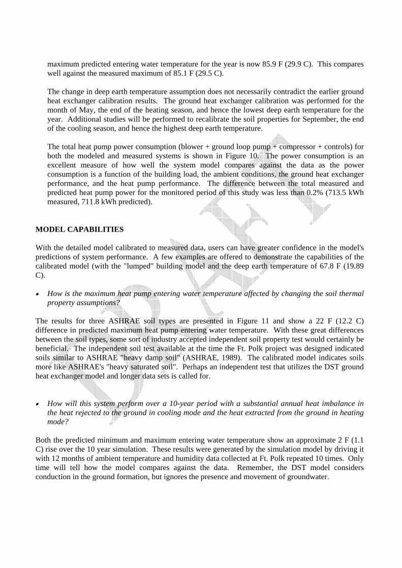
MODEL CAPABILITIES With the detailed model calibrated to measured data, users can have greater confidence in the model's predictions of system performance. A few examples are offered to demonstrate the capabilities of the calibrated model (with the "lumped" building model and the deep earth temperature of 67.8 F (19.89 C). • How is the maximum heat pump entering water temperature affected by changing the soil thermal

property assumptions? The results for three ASHRAE soil types are presented in Figure 11 and show a 22 F (12.2 C) difference in predicted maximum heat pump entering water temperature. With these great differences between the soil types, some sort of industry accepted independent soil property test would certainly be beneficial. The independent soil test available at the time the Ft. Polk project was designed indicated soils similar to ASHRAE "heavy damp soil" (ASHRAE, 1989). The calibrated model indicates soils more like ASHRAE's "heavy saturated soil". Perhaps an independent test that utilizes the DST ground heat exchanger model and longer data sets is called for. • How will this system perform over a 10-year period with a substantial annual heat imbalance in

the heat rejected to the ground in cooling mode and the heat extracted from the ground in heating mode?

Both the predicted minimum and maximum entering water temperature show an approximate 2 F (1.1 C) rise over the 10 year simulation. These results were generated by the simulation model by driving it with 12 months of ambient temperature and humidity data collected at Ft. Polk repeated 10 times. Only time will tell how the model compares against the data. Remember, the DST model considers conduction in the ground formation, but ignores the presence and movement of groundwater.

• If the ground heat exchangers were designed to be 20% shorter than originally proposed, what would be the heat pump entering water temperature consequences?

The length of the modeled ground heat exchanger was reduced by 20% (52 feet, 15.8 meters) per bore and the simulations run for the year. The simulation results for the 20% shorter case are compared with the installed depth simulation in Figure 12. Even with a 20% reduction in ground heat exchanger depth, the system did not exceed the commonly used design heat pump entering water temperature maximum of 95 F (35 C).

CONCLUSIONS A detailed component-based simulation of a GHP system has been calibrated to monitored data taken from a family housing unit at Ft. Polk, LA. The calibrated component models which comprise the system include the heat pump and its blower, the ground loop pump, the ground heat exchanger, the thermostat and the building load. The calibrated system model is then capable of addressing soil property impacts, multi-bore interactions, long-term consequences of annual heat imbalance, bore spacing, bore diameter, pipe spacing, pipe diameter, grout properties, and most other elements of vertical ground heat exchanger design. The outputs from this calibrated model at Ft. Polk can now be used to test the practical vertical ground heat exchanger design sizing programs. Further calibration exercises to monitored data are needed to demonstrate the capabilities and limitations of this new tool. REFERENCES ASHRAE Handbook of Fundamentals, 1977, 1981, 1985, 1985, 1993 Editions Ewbank and Associates, Thermal Test Results, Fort Polk Louisiana, October 1995 Hellstrom G. (1983) Heat Storage Subroutines in Minsun. Duct Storage Systems. Department of Mathematical Physics, University of Lund, Sweden. Hellstrom G. (1989) Duct Ground Heat Storage Model, Manual for Computer Code. Department of Mathematical Physics, University of Lund, Sweden. Hellstrom G., Mazzarella L. and Pahud D. (1996) Duct Ground Heat Storage Model. Lund - DST. TRNSYS 13.1 Version January 1996. Department of Mathematical Physics, University of Lund, Sweden. Hughes P. (1980) Improved Heat Pump Model for TRNSYS. Proceedings of the American Section of the Solar Energy Society. Kusuda, T., and Archenbach, P.R. "Earth Temperature amd Thermal Diffusivity at Selected Stations in the United States", ASHRAE Transactions, Vol. 71, Part 1, 1965 Klein S.A., et. al., TRNSYS Manual, "A Transient Simulation Program", Solar Energy Laboratory, University of Wisconsin, Version 14.2 for Windows, September 1996.

Mazzarella L. (1991) MINSUN 6.0 - NEWMIN 2.0. A Revised IEA Computer Program for Performance Simulation of Energy Systems with Seasonal Thermal Energy Storage. Proceedings Thermastock' 91, pp. 3.5-1 - 3.5-7, Scheveningen, The Netherlands. Mazzarella L. (1993) Duct Thermal Storage Model. Lund-DST. TRNSYS 13.1 Version 1993. ITW, Universitat Stuttgart, Germany, Dipartimento di Energetica, Politechnico di Milano, Italy. Pahud D., Hellstrom G. (1996) The New Duct Ground Heat Model for TRNSYS. Eurotherm Seminar N* 49, Eindhoven, The Netherlands, pp. 127-136. Pahud D., Fromentin A., Hadorn J.-C. (1996) The Duct Ground Heat Storage Model (DST) for TRNSYS Used for the Simulation of Energy Piles. User manual for the December 1996 version. Internal report. Laboratory of Energy Systems (LASEN), Swiss Federal Institute of Technology (EPFL), Lausanne, Switzerland. RIGHT-LOOP User's Manual, Wright Associates Inc., Version 1.00, September 1992. Typical Meteorological Year User's Manual TD - 9734, National Climatic Center, Asheville, North Carolina, May 1981.

TABLES

Heat ON Heat OFF Cool ON Cool OFF Note March 72.2 F

(22.3 C) 76.5 F (24.7 C)

N/A N/A

April 73.3 F (22.9 C)

76.2 F (24.6 C)

80.0 F (26.7 C)

76.3 F (24.6 C)

May N/A N/A 80.8 F (27.1 C)

77.2 F (25.1 c)

June N/A N/A 81.3 F (27.4 C)

76.8 F (24.9 C)

July N/A N/A 70.7 F (21.5 C)

70.7 F (21.5 C)

1

August N/A N/A 70.6 F (21.4 C)

70.6 F (21.4 C)

1, 2

September N/A N/A 77.0 F (25.0 C)

76.7 F (24.8 C)

3

October 78.6 F (25.9 C)

78.9 F (26.1 C)

N/A N/A

November 66.0 F (18.9 C)

68.2 F (20.1 C)

N/A N/A 4

Table 1: Monthly Thermostat Setpoints in Heating and Cooling Modes Table Notes:

1) The heat pump ran in each of the 15-minute recorded intervals for the entire month with no discernible room temperature differences found between when the equipment turned on and turned off.

2) The setpoint temperatures in August show three unique steps: a cooling setpoint of ~70 F for a very short period in the beginning of the month with no discernible turn-on and turn-off temperatures, a relatively long period where the space was maintained at ~74 F with no discernible turn-on and turn-off temperatures, and a short period at the end of the month where the space was maintained at ~62 F with no discernible turn-on and turn-off temperatures.

3) The setpoint temperatures in September shows a unique step: a short period where the cooling turn on temperature of ~64 F with a cooling turn off at ~64.5 F is observed followed by a relatively long period where the space is maintained at ~78 F with no discernible turn-on and turn-off temperatures.

4) The heat pump ran in only two of the 15-minute intervals for the month; making it impossible to determine the setpoints and deadbands.

258 Ft.

16 Ft.

25 Ft.

3 Ft.

(7.6 m)

(4.9 m)

(78.6 m)

(0.9 m)

4.125 Inches

2.57 Inches

1 Inch

(6.53 cm)

(2.54cm)

(10.48 cm)

Figure 1: Ground Heat Exchanger Configuration

Figure 2: Schematic of Modeled Ground Heat Pump System

0

5

10

15

20

25

30

35

40

45

50

1

101

201

301

401

501

601

701

801

901

1001

1101

1201

1301

1401

1501

1601

1701

1801

1901

2001

2101

2201

Interval

Pow

er (W

)

0

0.2

0.4

0.6

0.8

1

Rev

ersi

ng V

alve

Sta

tus

Heat Pump Power DrawReversing Valve Status

Figure 3: Controller Power Draw in Watts for Each 15-Minute Interval in the Month of April

60

65

70

75

80

85

90

1

118

235

352

469

586

703

820

937

1054

1171

1288

1405

1522

1639

1756

1873

1990

2107

2224

2341

2458

2575

2692

2809

2926

Interval

Tem

pera

ture

(F)

Cooling OnCooling Off

60

65

70

75

80

85

90

1

118

235

352

469

586

703

820

937

1054

1171

1288

1405

1522

1639

1756

1873

1990

2107

2224

2341

2458

2575

2692

2809

2926

Interval

Tem

pera

ture

(F)

Cooling OnCoolin Off

Figures 4 and 5: Room Temperatures for Cooling Turn-On and Turn-Off for the Months of May and August Respectively.

50

55

60

65

70

75

80

10.0

12.8

15.6

18.4

21.1

23.9

26.7

Model

Data

Figure 6: Predicted vs. Measured Heat Pump Entering Water Temperatures for Three Days in the

Month-Long Soil-Calibration Test

0.15

0.175

0.2

0.225

0.25

0.275

0.3

60 65 70 75 80 85 90

Entering Water Temperature (F)

Com

pres

sor

Ele

ctri

c C

onsu

mpt

ion

(kW

h)

DataCatalogModel

Figure 7: Energy Consumption of the Heat Pump Compressor as a Function of Heat Pump Entering

Water Temperature in Cooling Mode

0

3000

6000

9000

12000

15000

0.0

0.9

1.8

2.6

3.5

4.4

Ambient Temperature

Heating Data

Heating Model

Cooling Data

Cooling Model

Figure 8: Average Heating and Cooling Load Line Comparisons

60

65

70

75

80

85

90

15.6

18.4

21.1

23.9

26.7

29.4

32.2

Measured

Predicted

Figure 9: Predicted and Measured Maximum Heat Pump Entering Water Temperatures

0

100

200

300

400

500

600

700

Measured

Predicted

Figure 10: Predicted and Measured Heat Pump Power Consumption

50

60

70

80

90

100

110

10.0

15.6

21.1

26.7

32.2

37.8

43.3

Heavy Sat.

Heavy Damp

Heavy Dry

Figure 11: Maximum Heat Pump Entering Water Temperatures for Three Different Soil Types

50

60

70

80

90

100

10.0

15.6

21.1

26.7

32.2

37.8

Installed

20% Shorter

Figure 12: Predicted Maximum Heat Pump Entering Water Temperatures for a System with 20%

Shorter Ground Heat Exchangers than Installed.