Embed Size (px)
Citation preview

HELSINKI UNIVERSITY OF TECHNOLOGYFaculty of Electronics, Communications and AutomationDepartment of Signal Processing and Acoustics
Henri Korhola
Perceptual Study of Loudspeaker Crossover Filters
Master’s Thesis submitted in partial fulfilment of the requirements for the degree of Master ofScience in Technology.
Espoo, 25th February 2008
Supervisor: Professor Matti KarjalainenInstructor: Professor Matti Karjalainen

HELSINKI UNIVERSITY ABSTRACT OF THEOF TECHNOLOGY MASTER’S THESISAuthor: Henri KorholaName of the thesis: Perceptual Study of Loudspeaker Crossover FiltersDate: 25th February 2008 Number of pages: 81+10
Department: Signal Processing and AcousticsProfessorship: S-89
Supervisor: Prof. Matti KarjalainenInstructor: Prof. Matti Karjalainen
Digital signal processing offers interesting possibilities in audio reproduction. Crossover filter-ing in a multi-way loudspeaker is possible to implement digitally in a way that is not possiblewith analog filters. In spite of many publications on the topic, there exists few perceptualstudies of digital crossover filters.
This Master’s thesis presents an introduction to the theory of analog and digital filtering, prac-tical solutions of analog and digital crossover filters and discusses the differences among them.Later in the thesis, a perceptual study is conducted with two digital crossover filters: digitallinear-phase FIR crossover filter and a digital implementation of the analog, so called Linkwitz-Riley crossover filter. The experiment was carried out as a listening experiment using bothheadphone simulation and a real loudspeaker in a listening room. The main goal of the studywas to find out the Just Noticeable Difference (JND) limits for phase errors caused by thecrossover filters with different sound samples.
The results of the listening experiment were analysed with auditory correlates of group delaydistortion (phase errors) and smoothed third-octave spectrum (magnitude error). These corre-lates explain the results of the listening tests to some extent, but with high-order linear-phaseFIR crossover filters, correlation seemed not to always exist. Thus auditory analysis that wasbased on the function of hearing was used for analysis. It seemed to show qualitatively thereasons for perceived phase errors.
It was discovered that high-order, linear-phase FIR crossover filters offer apparently ”ideal”properties in magnitude and phase reproduction for crossover filters, but they cause clearlyaudible degradations as ”ringing” in the audio samples, when the flight-time difference betweenlow- and highpass outputs is not zero. The crossover frequency between low- and highpassbands being 3 kHz, it was noticed on the grounds of the listening experiments that filter ordersabove 600 produce audible errors with linear-phase FIR crossover filters.
Keywords: DSP, digital audio, crossover filters, FIR, psychoacoustics, perception, phase dis-tortion, group delay
i
TEKNILLINEN KORKEAKOULU DIPLOMITYÖN TIIVISTELMÄTekijä: Henri KorholaTyön nimi: Perceptual Study of Loudspeaker Crossover FiltersPäivämäärä: 25.2.2008 Sivuja: 81+10
Laitos: Signaalinkäsittelyn ja akustiikan laitosProfessuuri: S-89
Työn valvoja: Prof. Matti KarjalainenTyön ohjaaja: Prof. Matti Karjalainen
Digitaalinen suodatus tarjoaa kiinnostavia mahdollisuuksia äänentoistossa. Monitiekaiuttimienjakosuotimien digitaalinen toteutus on mahdollista suodinratkaisuilla, jotka eivät analogisis-sa suotimissa ole mahdollisia. Digitaalijakosuotimista on julkaistu monia artikkeleita, muttahavaintotutkimukset ovat harvassa.
Diplomityössä on esitelty analogisen ja digitaalisen suodatuksen teoriaa, käytännön ratkaisuja,sekä pohdittu eroja menetelmien välillä. Työssä on myöhemmin tutkittu monitiekaiuttimien di-gitaalisten jakosuodinten ominaisuuksia kahdella eri jakosuodintyypillä: digitaalisella lineaari-vaiheisella FIR-jakosuotimella sekä niin kutsutun Linkwitz-Riley analogisen jakosuotimen di-gitaalisella toteutuksella. Tutkimus suoritettiin havaintotutkimuksena kuuntelukokeiden avullasekä kuulokesimulaationa että oikealla kaiuttimella kuunteluhuoneessa. Tavoitteena oli selvit-tää jakosuotimien aiheuttamien vaihevirheiden havaittavuutta ja niiden havaintokynnyksiä eriääninäytteillä.
Tuloksia analysoitiin auditoristen korrelaattien, ryhmäviivepoikkeaman (vaihevirhe) ja peh-mennetyn terssikaistaspektrin (magnitudivirhe) avulla. Nämä korrelaatit selittävät havaittujailmiöitä tiettyyn pisteeseen asti, mutta lineaarivaiheisten FIR-jakosuotimien tapauksessa kor-relaatiota ei aina esiintynyt. Tämän vuoksi tutkimuksen loppuvaiheessa tuloksia analysoitiinkuulon toimintaan perustuvan auditorisen analyysin avulla, mikä selittää ilmiöt kvalitatiivises-ti.
Tutkimuksen perusteella havaittiin, että korkean asteen lineaarivaiheiset FIR-jakosuotimet tar-joavat näennäisesti ”ideaaliset” jakosuotimen ominaisuudet sekä vaihe- että magnituditoistonosalta, mutta aiheuttavat selvästi kuultavia häiriötä (”soimista”) ääninäytteisiin, kun aikaeromatalien ja korkeiden taajuuksien kaiutinelementtien välillä ei ole nolla. Matalien ja korkeidentaajuuksien kaistojen jakotaajuuden ollessa 3 kHz havaittiin, että yli 600 asteen lineaarivaihei-set FIR-jakosuotimet näyttävät aiheuttavan selkeitä häiriötä ääneen sekä kuulokesimulaatioidenettä oikean kaiutinkokeen perusteella.
Avainsanat: digitaalinen suodatus, digitaaliaudio, monitiekaiutin, jakosuodin, FIR, psykoakus-tiikka, ryhmäviivepoikkeama, vaihevirhe
ii

Preface
This Master’s thesis has been done for the Acoustics and Audio Signal Processing Laboratory atHelsinki University of Technology during the years 2007-2008. It has been an interesting projectin the audio and psychoacoustics fields. I am grateful for the financial support of TKK that madethe thesis possible.
First, I want to thank my supervisor and instructor of the thesis, professor Matti Karjalainen.His devotion to acoustics and interaction capabilities make a superb combination, which I hadthe pleasure enjoying. The whole staff at the Acoustics Laboratory deserve a praise, as well.Especially Mr. Martti Rahkila, who struggled to find me a good working environment. It is hardto imagine a better place to write a thesis.
Last, my eventually deepest gratitude is directed to my beloved family, friends and to my darling.Thank you all for your many-sided support and presence. Immersing in my work was both easyand pleasant as the surroundings were great around me.
Tontunmäki, 25th February 2008
Henri Korhola
iii

Contents
Abbreviations viii
1 Introduction 1
2 Overview of Loudspeaker Technology 3
2.1 Reproducing Sound . . . . . . . . . . . . . . . . . . . . . . . . . . . . . . . . 3
2.2 Drivers . . . . . . . . . . . . . . . . . . . . . . . . . . . . . . . . . . . . . . 4
2.2.1 Introduction . . . . . . . . . . . . . . . . . . . . . . . . . . . . . . . . 4
2.2.2 Dynamic Driver . . . . . . . . . . . . . . . . . . . . . . . . . . . . . . 4
2.2.3 Equivalent Circuit of Dynamic Driver . . . . . . . . . . . . . . . . . . 4
2.3 Enclosures . . . . . . . . . . . . . . . . . . . . . . . . . . . . . . . . . . . . . 6
2.3.1 Closed Box . . . . . . . . . . . . . . . . . . . . . . . . . . . . . . . . 6
2.3.2 Bass-Reflex Box . . . . . . . . . . . . . . . . . . . . . . . . . . . . . 6
2.4 Room Effects . . . . . . . . . . . . . . . . . . . . . . . . . . . . . . . . . . . 7
2.5 Crossover Filters . . . . . . . . . . . . . . . . . . . . . . . . . . . . . . . . . 8
3 Crossover Filters 9
3.1 Analog and Digital Filtering . . . . . . . . . . . . . . . . . . . . . . . . . . . 9
3.1.1 Laplace-, Fourier- and Z-transform . . . . . . . . . . . . . . . . . . . 9
3.1.2 Transfer Function . . . . . . . . . . . . . . . . . . . . . . . . . . . . . 10
3.1.3 Frequency Response . . . . . . . . . . . . . . . . . . . . . . . . . . . 11
3.1.4 Filter Types by Frequency Response Characteristics . . . . . . . . . . 12
3.2 Crossover Filters . . . . . . . . . . . . . . . . . . . . . . . . . . . . . . . . . 13
3.2.1 Transfer Function of Crossover Filter . . . . . . . . . . . . . . . . . . 14
iv
3.2.2 Butterworth Type Crossovers . . . . . . . . . . . . . . . . . . . . . . . 15
3.2.3 Linkwitz-Riley Type Crossovers . . . . . . . . . . . . . . . . . . . . . 16
3.2.4 FIR Type Filters . . . . . . . . . . . . . . . . . . . . . . . . . . . . . 17
3.2.5 Goal of Crossover Design . . . . . . . . . . . . . . . . . . . . . . . . 18
3.3 Passive Crossover Filters . . . . . . . . . . . . . . . . . . . . . . . . . . . . . 19
3.3.1 Advantages . . . . . . . . . . . . . . . . . . . . . . . . . . . . . . . . 19
3.3.2 Drawbacks and Problems . . . . . . . . . . . . . . . . . . . . . . . . . 20
3.4 Active Crossover Filters . . . . . . . . . . . . . . . . . . . . . . . . . . . . . 21
3.4.1 Advantages and Drawbacks . . . . . . . . . . . . . . . . . . . . . . . 22
3.4.2 Practical Solutions . . . . . . . . . . . . . . . . . . . . . . . . . . . . 23
3.5 Digital Crossover Filters . . . . . . . . . . . . . . . . . . . . . . . . . . . . . 24
3.5.1 Advantages . . . . . . . . . . . . . . . . . . . . . . . . . . . . . . . . 24
3.5.2 Drawbacks and Problems . . . . . . . . . . . . . . . . . . . . . . . . . 25
3.5.3 Practical Solutions . . . . . . . . . . . . . . . . . . . . . . . . . . . . 26
3.6 Summary of Crossover Filters . . . . . . . . . . . . . . . . . . . . . . . . . . 27
4 Psychoacoustics 29
4.1 Auditory System . . . . . . . . . . . . . . . . . . . . . . . . . . . . . . . . . 30
4.2 Timbre and Colouration . . . . . . . . . . . . . . . . . . . . . . . . . . . . . . 32
4.3 Perception of Spectral Properties . . . . . . . . . . . . . . . . . . . . . . . . . 32
4.3.1 Frequency Masking . . . . . . . . . . . . . . . . . . . . . . . . . . . . 33
4.3.2 Critical Band and Frequency Selectivity . . . . . . . . . . . . . . . . . 33
4.3.3 Frequency Sensitivity and Loudness . . . . . . . . . . . . . . . . . . . 35
4.4 Perception of Temporal Properties . . . . . . . . . . . . . . . . . . . . . . . . 36
4.4.1 Temporal Masking . . . . . . . . . . . . . . . . . . . . . . . . . . . . 36
4.4.2 Perception of Timbre . . . . . . . . . . . . . . . . . . . . . . . . . . . 37
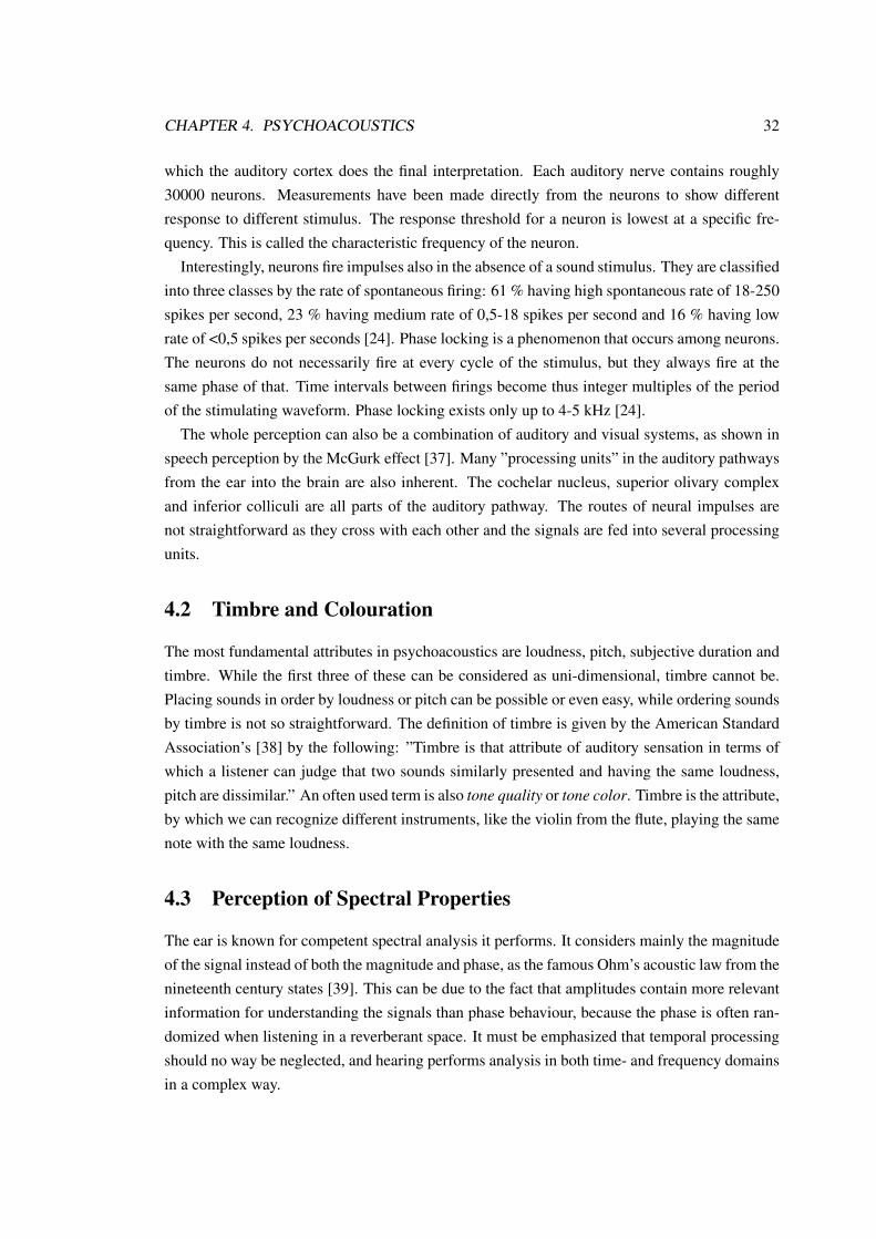
4.5 Perception of Spatial Properties . . . . . . . . . . . . . . . . . . . . . . . . . . 38
5 Listening Experiment 41
5.1 Motivation and Goals . . . . . . . . . . . . . . . . . . . . . . . . . . . . . . . 41
5.2 Description of Listening Test . . . . . . . . . . . . . . . . . . . . . . . . . . . 41
v

5.2.1 Test Procedure . . . . . . . . . . . . . . . . . . . . . . . . . . . . . . 41
5.2.2 Test Material and Parameters . . . . . . . . . . . . . . . . . . . . . . . 42
5.2.3 Test Equipment . . . . . . . . . . . . . . . . . . . . . . . . . . . . . . 44
5.3 Results of Simulated Loudspeaker Test . . . . . . . . . . . . . . . . . . . . . . 44
5.3.1 Results of FIR Crossover Filters . . . . . . . . . . . . . . . . . . . . . 45
5.3.2 Results of Linkwitz-Riley Crossover Filters . . . . . . . . . . . . . . . 46
5.4 Analysis . . . . . . . . . . . . . . . . . . . . . . . . . . . . . . . . . . . . . . 46
5.4.1 Magnitude Errors of L-R Crossover Filters . . . . . . . . . . . . . . . 49
5.4.2 Group Delay Errors of L-R Crossover Filters . . . . . . . . . . . . . . 49
5.4.3 Group Delay Errors of FIR Crossover Filters . . . . . . . . . . . . . . 50
5.4.4 Ringing Phenomenon of FIR Crossover Filters . . . . . . . . . . . . . 52
5.4.5 Effect of Training . . . . . . . . . . . . . . . . . . . . . . . . . . . . . 57
5.5 Results and Analysis of Loudspeaker Listening Experiment . . . . . . . . . . . 58
5.6 Conclusions from the Listening Experiments . . . . . . . . . . . . . . . . . . . 60
6 Auditory Analysis 61
6.1 Different Auditory Models . . . . . . . . . . . . . . . . . . . . . . . . . . . . 61
6.1.1 Psychoacoustical Spectrum Models . . . . . . . . . . . . . . . . . . . 62
6.1.2 Filterbank Models . . . . . . . . . . . . . . . . . . . . . . . . . . . . 62
6.1.3 Cochlear Models . . . . . . . . . . . . . . . . . . . . . . . . . . . . . 63
6.2 Auditory Analysis of the Listening Test . . . . . . . . . . . . . . . . . . . . . 64
6.2.1 Structure of Filterbank Model . . . . . . . . . . . . . . . . . . . . . . 64
6.2.2 Auditory Response to 10 Hz Square Wave . . . . . . . . . . . . . . . . 65
6.2.3 Auditory Response to Castanets . . . . . . . . . . . . . . . . . . . . . 68
6.2.4 Conclusions from Auditory Analysis . . . . . . . . . . . . . . . . . . 70
7 Conclusions and Future Work 74
A Listening Test Graphical User Interface 82
B Results of the listening test 84
C Results of the listening test as table 88
vi

D Results of Real Loudspeaker Experiment 91
vii

Abbreviations
BM Basilar MembranedB decibelDSP Digital Signal ProcessingDFT Discrete Fourier TransformDTFT Discrete-time Fourier TransformERB Equivalent Rectangular BandwidthFFT Fast Fourier TransformFIR Finite Impulse ResponseHRTF Head-related Transfer FunctionHz HertzIIR Infinite Impulse ResponseILD Interaural Level DifferenceITD Interaural Time DifferenceJND Just Noticeable DifferenceL-R Linkwitz-Rileyms millisecondTM Tectorial Membrane
viii
Chapter 1
Introduction
Digital Signal Processing (DSP) technology has come to stay and it offers an interesting varietyof possibilities also in the audio world. The quest for perfect reproduction of sound continuesand open-mindedness is required by accepting the advantages of digital processing of sound.Nowadays the information chain from recording sound signals to the very end of creating thesound pressure fluctuations by a loudspeaker is often digital, hence creating a distinct demandfor digital technology in loudspeakers.
As the physical limitations come into play when trying to cover the entire audio range from thebass range to the high frequencies, reproducing sound waves needs different types of loudspeakerelements (i.e. drivers) for different kinds of sounds. Splitting the audio range for proper drivers isneeded, and this job is done by crossover filters. Until very recently, loudspeaker designers haveused analog technology to do this assignment. However, the development of DSP technologyoffers considerable options for filtering the sound signals and directing the right signals to theright drivers effectively and precisely.
Filtering can be done either passively or actively. Passive filters consist of passive electric cir-cuits, whereas active filters can more freely manipulate the signal by, for example, amplifying it.With digital filtering, new features, such as different filter properties, cheaper mass-production,good adjustability, and on-site equalization (”correction”) of reproduction, become possible. Un-fortunately, they are not coming without side effects. Filtering sound digitally may cause subtlechanges in signals, and the audibility of those changes has been under discussion since the in-troduction of digital technology to the audio world. This thesis will investigate the perceptionof these subtle changes due to digital filtering by simulating crossover filters. A listening test isplanned and conducted to find out differences in digital crossover filters’ effect on sound qualityand to obtain approximate audibility limits for certain errors. Reasons for errors are tried to findand explain with auditory analysis.
The thesis consists of seven chapters. After this introduction, an overview of loudspeakertechnology is given in Chapter 2. A deeper insight into crossover filters and their structure andfunction is given in Chapter 3. The science of psychoacoustics studies the perception of sound,
1
CHAPTER 1. INTRODUCTION 2
and it is thus essential for understanding the whole perception chain from a loudspeaker to thebrain, which eventually produces the listening experience. Psychoacoustics and its essentials forthis thesis are dealt with in Chapter 4. A listening test on differences in digital crossover filtersand their effect on sound quality is presented in Chapter 5, including results and discussion onthe topic. The concept of an auditory model is introduced in Chapter 6. Auditory analysis basedon auditory models is used for further analysis as well as for trying to predict the results ofthe listening test. Finally, conclusions of this study are given in Chapter 7. Bibliography andAppendices are located at the end of the thesis.
Chapter 2
Overview of Loudspeaker Technology
Loudspeakers are designed to reproduce recorded sound signals in the listening environment.They act as the last, and often the weakest link between electric signals and real, audible sound.They are electro-mechanic-acoustic transducers, which create sound pressure fluctuations intothe air from input signals. This task is demanding due to the physical features of sound.
In general, sound reproduction has come all the way from the good old gramophones to state-of-the-art DSP loudspeaker systems in a period of less than a hundred years. The first modern-kind devices were introduced to public during the 1920s, and High-Fidelity (Hi-Fi) reproductionwith two channels (stereo) came into public knowledge in the 1950s. The revolution of digitalaudio with CDs dates back to the 1980s. The quality of loudspeakers was not good by the modernstandards until the 1950s. Since the introduction of CD-players in 1980, it can be said that Hi-Fiquality sound reproduction has been available to everybody, not just to the upper class [1].
2.1 Reproducing Sound
The ratio of air pressure fluctuations between the just noticeable sound and a very high soundpressure level can be as big as 1:1 000 000. This sets unparalleled difficulties for loudspeakersin covering the entire frequency range from 20 to 20000 Hz, which is approximately the hearingrange of humans. Hence, different kinds of loudspeaker elements (drivers) are needed. Creatingsound waves at low frequencies below 100 Hz demands a woofer, which is a physically largedriver, whereas high frequencies from roughly 1-5 kHz up to 20 kHz can be reproduced with asmall, fast vibrating tweeter [1].
A multi-way loudspeaker, which has multiple drivers for different frequency ranges, was in-troduced to public in the 1930s by Bell Laboratories and its principle is used in the present day’sloudspeakers. Using more than one driver creates a problem: how not to feed an improper signal,which the driver is not capable of reproducing, into it? The answer is called the crossover filter,which is an electric circuit that filters the right frequencies to the right drivers. Due to theserequirements, we are faced with one of the fundamental problems in loudspeakers design.
3
CHAPTER 2. OVERVIEW OF LOUDSPEAKER TECHNOLOGY 4
2.2 Drivers
2.2.1 Introduction
Drivers come in many flavors: there are electrodynamic, electrostatic, piezoelectric, horn andribbon drivers. The dynamic, moving-coil driver is by far the most common of these, and theother types are of interest in this thesis. The moving coil loudspeaker was developed by E.W.Kellogg and C. W. Rice and their first commercial product was named ”Radiola 104” [1]. It waslaunched on the market in 1926.
2.2.2 Dynamic Driver
The principle of a dynamic driver is shown in Figure 2.1. It works by the following method: apower amplifier acting as a voltage source creates an alternating current in the driver’s voice coil.This creates an alternating force, which moves the diaphragm that correspondingly replaces airand creates the sound waves that we can hear [2]. The physics behind the two-way connectionbetween electrical and mechanical components are given by:
F = Bli (2.1)
U = Blv (2.2)
where i is the current in the voice coil, F is the force, B is the magnetic flux density in whichthe voice coil is immersed, l is the effective length of voice coil in this magnetic field, U is thevoltage, and v is the velocity of voice coil.
The dynamic element loudspeaker is a usual choice as well for commonplace loudspeakersas for Hi-Fi. Its reproduction quality can be made good, even though the efficiency rate is poor.Only about 1 per cent of the electrical power is transformed into acoustic power.
2.2.3 Equivalent Circuit of Dynamic Driver
Physics includes useful analogues for expressing different components in a unified way to makeproper analysis and to understand things better. Transforming electrical energy to mechanicaland further to acoustic energy can be presented as an electric circuit. Figure 2.2 presents theimpedance equivalent circuit for electro-mechanic-acoustic analogue of a loudspeaker driver.Impedance analogue means that mechanical quantities of force F and velocity u are expressedin electrical quantities as voltage V and current i, respectively [1].
The circuit is driven by a power amplifier, which is modeled by an alternating current (AC)voltage source. The resistance and inductance of the voice coil are modeled by resistor Rc andinductor Lc, correspondingly. In theory, electrical energy is ideally transformed to mechanicalby a transformer of turns ratio Bl : 1, in which B is the density of magnetic flux for the voicecoil and l is the effective length of the voice coil in the magnetic field. This ratio is known as theforce factor.

CHAPTER 2. OVERVIEW OF LOUDSPEAKER TECHNOLOGY 5
Figure 2.1: Cut of electrodynamic driver. The voice coil moving in the magnet field createsmotion to the diaphragm that replaces air molecules.
The middle section of the model is the mechanical section in which mass, mechanical resis-tance, and compliance (inverse of stiffness) of the driver are expressed as Mad, Rad and Cad.
Finally, mechanical energy is ideally transformed to acoustic energy by a transformer of turnsratio 1 : Sd, where Sd is the area of the loudspeaker diaphragm. The acoustic impedances in thefront of and behind the diaphragm are expressed as Za. Now further design, analysis, and studyhave been made easier using the model.
Figure 2.2: Equivalent circuit of electrodynamic driver. [1]

CHAPTER 2. OVERVIEW OF LOUDSPEAKER TECHNOLOGY 6
Figure 2.3: Closed box. Figure 2.4: Equivalent circuit of closedbox.[1]
2.3 Enclosures
An essential part of a loudspeaker is the enclosure. After the driver has created pressure differ-ences in the air (sound waves), they should be directed properly in order to make audible soundinstead of creating destructive interaction between the sound waves in both sides of the driver.Typical solutions are closed boxes and bass-reflex boxes.
Designing an enclosure needs specifying different variables: the driver; the material of the en-closure, its volume and stiffness, etc. All these have to be planned to avoid unwanted resonancesand diffraction from the edges of the enclosure. Typical materials are different types of wood,plastic, steel and even rock. A prevailing choice is to use MDF (Medium Density Fibreboard) asthe loudspeaker material.
2.3.1 Closed Box
A closed box represents a common solution of enclosing the driver. There are no openings inthe box, just the driver radiating sound. Figure 2.3 and Figure 2.4 present a closed enclosure andits electrical equivalent circuit. Rab is the resistivity, Vb is the enclosed volume, γ is the ratio ofheats for air, and Ps is the static pressure [1].
2.3.2 Bass-Reflex Box
Another common enclosure is the bass-reflex box. It is also referred to as a ported or a ventedbox due to a port or a vent in the enclosure. This air tube causes the bass-reflex enclosure actas a Helmholtz resonator, which means that the air mass in the tube resonates together withthe air spring in the enclosure at a specific Helmholtz frequency, thus providing a greater bassreproduction with smaller volume enclosures and reducing the excursion of the driver in theproximity of the resonant frequency.
Figure 2.5 shows a bass-reflex box and Figure 2.6 its equivalent circuit, in which k is the wavenumber (2π/λ), ρ is the density of air, c is the speed of sound in air, Leff is the effective lengthof the air tube in the bass-reflex box, a is the radius of the same tube, Rab is the resistivity as inthe closed box case, Vb is the enclosed volume, and γ is the ratio of heats for air [1].

CHAPTER 2. OVERVIEW OF LOUDSPEAKER TECHNOLOGY 7
Figure 2.5: Vented box. Figure 2.6: Equivalent circuit of ventedbox.[1]
2.4 Room Effects
An integral part of a sound reproduction system is the listening room, excluding headphonelistening. It has a strong effect on the quality of reproduction, and it must not be forgotten thatthe reproduction chain includes also the environment, not only the electric reproduction devices.The analysis of the room’s effect by mathematical functions is demanding and complicated.
There are certain phenomena and certain parameters in room acoustics, which have to beunderstood and taken into account. Standing waves are formed in a room, and they have apowerful effect on the sound field created. They are waves of the same wavelength travelling inopposite directions in a room. This causes interference between the waves, and sound is eitherweakened or strengthened, depending on the observation point.
Room modes are standing waves formed in the room at the natural resonance frequencies ofthe room. The modes depend on the combinations of room dimensions. Lord Rayleigh [3]derived an equation, which gives the frequencies of a rectangular room modes by:
f =c
2
√[nll
]2+[nww
]2+[nhh
]2(2.3)
where nl, nw, nh are integers and l,w,h are the length, width and height of the room.As sound is emitted from sound source to receiver, first the direct sound is perceived. Second,
the early reflections come from nearby surfaces. Finally, the late reflections from other surfacesarrive as reverberation.
Reverberation tells how long the sound field exists after the sound source has stopped emittingsound. As materials absorb and reflect sound diversely, there are big differences in reverberationtimes. Reverberation is the main design parameter in room acoustics, and usually the reverbera-tion time is given as the time, in which sound level has decreased by the factor of 1000, i.e. 60dB. Sabine defined the equation for calculating T60 by [4]:
T60 =0.161VA
(2.4)
where V is the room volume and A is the total absorption area in the room by different materialsand surfaces.

CHAPTER 2. OVERVIEW OF LOUDSPEAKER TECHNOLOGY 8
Flutter echo is a specific reverberation, which occurs between reflective, parallel surfaces asthe sound waves reflect repeatedly between the surfaces with a short delay. Hearing detectsdiscretely the decaying impulses and thus a flutter echo is perceived. It is a common problem ina room with a small amount of damping material and hard, opposite walls. [4].
2.5 Crossover Filters
Physics sets the limits for reproduction systems and compromises have to be made. As noloudspeaker driver can reproduce all the audible frequencies from 20 Hz to 20 kHz in a decent,errorless way, splitting the spectrum for multiple drivers is required by an audio crossover filter.It is an electric filter, which can either be passive without an external power supply, or activewith an external power supply. The active filter can add gain to signal and use external energy.Digital crossover filters have also made their entrance and new, interesting solutions have becomepossible due to digital signal processing. Digital crossover filters can be either digital simulationsof analog filters or purely digital filters that do not have analog counterparts.
An ideal crossover filter would filter exactly the defined frequencies to the woofer and respec-tively to the tweeter, so that no overlapping between the drivers would emerge and interfere witheach other. It would as well keep the filtered, summed output signal from the woofer and tweeterintact in terms of magnitude and phase. In reality, such filter is not possible due to physicallimitations.
After having presented an overview of loudspeaker technology in this chapter, we will nextdiscuss crossover filters in details. Comparison is made between active and passive analogcrossovers. Also a deeper insight into digital crossover filters is given. They are the most inter-esting part of the thesis. The properties of digital filters are studied and their influence on thequality of sound is discussed.
Chapter 3
Crossover Filters
Loudspeaker crossover filters are needed for good sound reproduction, but at the same time manyproblems exist. In this chapter the theoretical basis of loudspeaker crossover filters is given byfirst introducing the concept of filtering in the analog and the digital domains and continuingto crossover filters. After the mathematical and physical background, different realizations andsome practical solutions of crossover filters are presented in their passive and active forms. Fi-nally, the use of digital technology in crossover filters is discussed.
3.1 Analog and Digital Filtering
3.1.1 Laplace-, Fourier- and Z-transform
In system analysis, the concept of filtering is essential. Filtering can be thought as changingthe relative amplitudes and phases of frequency components or perhaps eliminating some com-ponents. A transformation from the time domain to the frequency domain is usually applied infilter analysis. It means representing the time signal as weighted sum of complex components,either in complex form or in polar (exponential) form. In the continuous-time analog world,the transformation is done by the Laplace transform or the Fourier transform, whereas in thediscrete-time digital world it is done by the Z-transform or the discrete-time Fourier transform(DTFT). The transforms are defined by the following equations [5]:
X(s) =∫ ∞−∞
x(t)e−stdt Laplace (3.1)
X(ω) =∫ ∞−∞
x(t)e−jωtdt Fourier (3.2)
where s is the complex frequency variable α+ ωj (where j is the imaginary unit and ω is 2πf ),and for discrete-time respectively:
X(z) =∞∑
n=−∞x(n)z−n Z− transform (3.3)
9

CHAPTER 3. CROSSOVER FILTERS 10
X(z) =∞∑
n=−∞x(n)e−jωn DTFT (3.4)
where z = rejω, in which r is the magnitude, j is the imaginary unit and ω is 2πf .
3.1.2 Transfer Function
Now we can conveniently express signals in either the s-domain or the z-domain. Because ofthe convolution property, the input and output of a linear, time-invariant system (LTI) have arelationship, which is characterised by the system’s transfer function [5]:
H(s) =Y (s)X(s)
(3.5)
and for discrete-time, digital domain:
H(z) =Y (z)X(z)
(3.6)
The transfer function is also called the system function [5]. A block diagram presentation isshown in Figure 3.1.
Figure 3.1: Block diagram of a filter and its transfer function. Transfer function is the ratio ofoutput and input signals.
Since many systems are described by linear, constant-coefficient differential equations in theanalog domain and corresponding difference equations in the digital domain, applying Laplace-or Z-transform to both sides of the equations gives the following:
N∑k=0
akskY (s) =
M∑k=0
bkskX(s) (3.7)
andN∑k=0
akz−kY (z) =
M∑k=0
bkz−kX(z) (3.8)
From Equation (3.5) the general form of transfer function can be presented as the ratio of twopolynomials [5]:
H(s) =∑M
k=0 bksk∑N
k=0 aksk
(3.9)
CHAPTER 3. CROSSOVER FILTERS 11
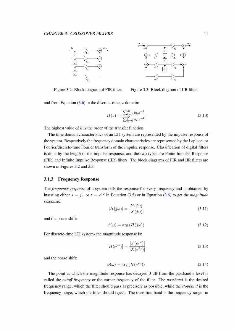
Figure 3.2: Block diagram of FIR filter. Figure 3.3: Block diagram of IIR filter.
and from Equation (3.6) in the discrete-time, z-domain:
H(z) =∑M
k=0 bkz−k∑N
k=0 akz−k
(3.10)
The highest value of k is the order of the transfer function.The time domain characteristics of an LTI system are represented by the impulse response of
the system. Respectively the frequency domain characteristics are represented by the Laplace- orFourier/discrete-time Fourier transform of the impulse response. Classification of digital filtersis done by the length of the impulse response, and the two types are Finite Impulse Response(FIR) and Infinite Impulse Response (IIR) filters. The block diagrams of FIR and IIR filters areshown in Figures 3.2 and 3.3.
3.1.3 Frequency Response
The frequency response of a system tells the response for every frequency and is obtained byinserting either s = jω or z = ejω in Equation (3.5) or in Equation (3.6) to get the magnituderesponse:
|H(jω)| = |Y (jω)||X(jω)|
(3.11)
and the phase shift:φ(ω) = arg (H(jω)) (3.12)
For discrete-time LTI systems the magnitude response is:
∣∣H(ejω)∣∣ =
∣∣Y (ejω)∣∣
|X(ejω)|(3.13)
and the phase shift:φ(ω) = arg (H(ejω)) (3.14)
The point at which the magnitude response has decayed 3 dB from the passband’s level iscalled the cutoff frequency or the corner frequency of the filter. The passband is the desiredfrequency range, which the filter should pass as precisely as possible, while the stopband is thefrequency range, which the filter should reject. The transition band is the frequency range, in

CHAPTER 3. CROSSOVER FILTERS 12
which the magnitude response goes from the passband to the stopband. These properties can beobserved later from Figure 3.4 on Page 13.
From the Equations (3.12) (and 3.14) we can derive the concepts of phase delay and groupdelay. The phase delay tells the frequency-dependent delay to a sinusoid by:
τφ(ω) =−φ(ω)ω
(3.15)
whereas the group delay tells the rate of change by the first derivative of phase shift in respect tofrequency:
τg(ω) =−dφ(ω)dω
(3.16)
From the frequency response we can find out the changes in the magnitude and the phasecompared to the input signal. The frequency response plays a major role in, for example, audiosystem analysis. The main interest is usually laid on the magnitude response, but the phaseresponse should not be neglected. The gain G in the magnitude response is given in decibels bythe definition:
G[dB] = 20 log10
(V
V0
)(3.17)
where V is the voltage level and V0 is the reference voltage level.The group delay is a commonly used measure of phase distortion in crossover filter analysis
telling how much a certain frequency component or frequency range of a signal is delayed. It iscalled also the envelope delay as it tells how much the envelope curve of a complex signal thatcontains many frequencies is delayed. It is usually given in either samples or in milliseconds.
3.1.4 Filter Types by Frequency Response Characteristics
Filters can be divided into several groups by their transfer function type. The properties of afilter are always trade-offs from each other, which means that a flat magnitude response cancause slow roll-off after the required cutoff frequency, or deep damping in the stopband cancause magnitude ripple in the filter’s passband. Common filter types and their properties arepresented in Table 3.1. The first three are analog filters, which would be implemented with IIRfilter types in the digital domain, and the last two are digital filters.
Filter type PropertiesButterworth Maximally flat passband, slow attenuation
Bessel Minimal group delay errors, flat passband, slow attenuation
Elliptic Ripple in pass- and stopband, fast attenuation
Digital FIR Linear phase possible, adds delay, moderate attenuation per order
Digital IIR Non-linear phase, fast attenuation per order
Table 3.1: Common filter types
CHAPTER 3. CROSSOVER FILTERS 13
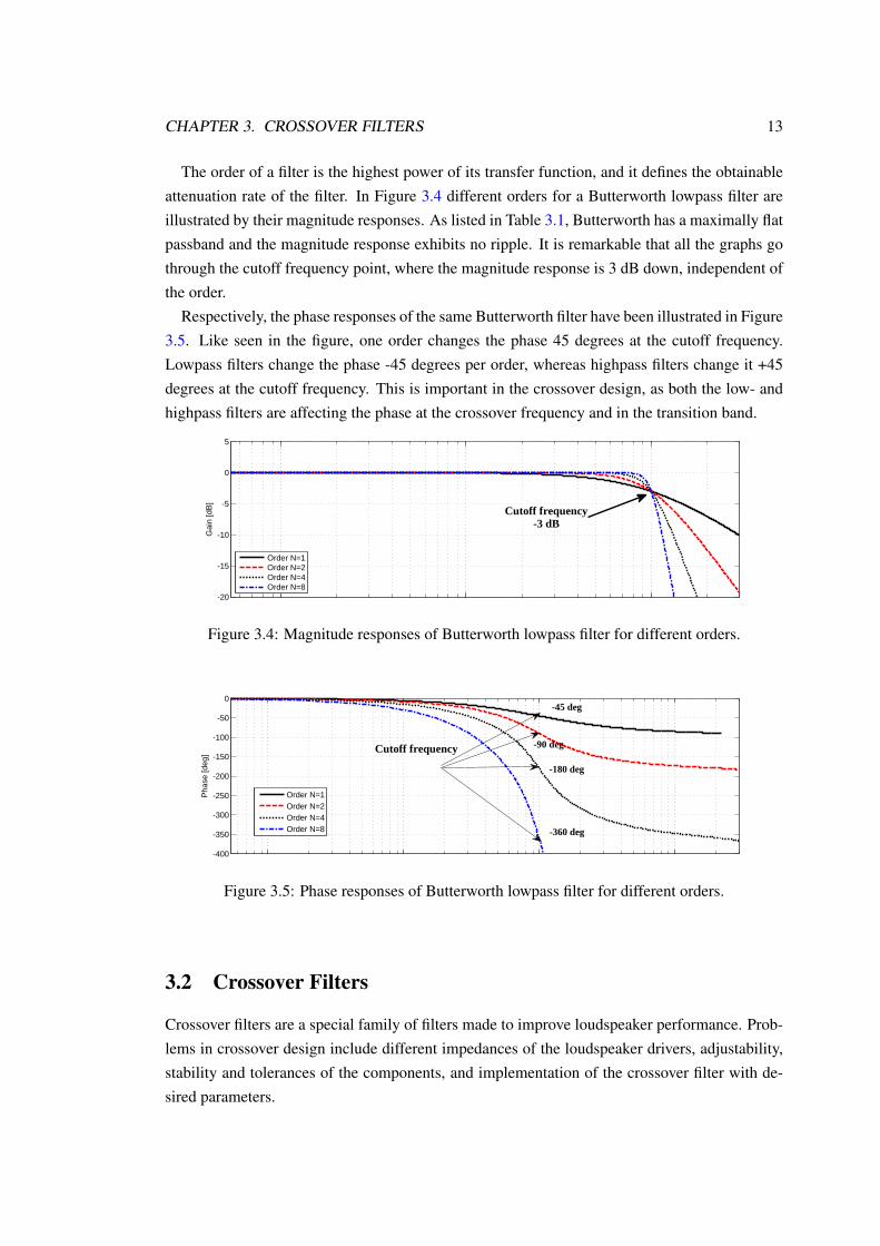
The order of a filter is the highest power of its transfer function, and it defines the obtainableattenuation rate of the filter. In Figure 3.4 different orders for a Butterworth lowpass filter areillustrated by their magnitude responses. As listed in Table 3.1, Butterworth has a maximally flatpassband and the magnitude response exhibits no ripple. It is remarkable that all the graphs gothrough the cutoff frequency point, where the magnitude response is 3 dB down, independent ofthe order.
Respectively, the phase responses of the same Butterworth filter have been illustrated in Figure3.5. Like seen in the figure, one order changes the phase 45 degrees at the cutoff frequency.Lowpass filters change the phase -45 degrees per order, whereas highpass filters change it +45degrees at the cutoff frequency. This is important in the crossover design, as both the low- andhighpass filters are affecting the phase at the crossover frequency and in the transition band.
101
102
103
-20
-15
-10
-5
0
5Amplitude response of Butterworth low pass filter with cutoff at 1 kHz
Gai
n [d
B]
Frequency [Hz]
Order N=1Order N=2Order N=4Order N=8
Cutoff frequency-3 dB
Figure 3.4: Magnitude responses of Butterworth lowpass filter for different orders.
101
102
103
104
-400
-350
-300
-250
-200
-150
-100
-50
0Phase response of Butterworth low pass filter with cutoff at 1 kHz
Pha
se [d
eg]
Frequency [Hz]
Order N=1Order N=2Order N=4Order N=8
Cutoff frequency
-360 deg
-180 deg
-45 deg
-90 deg
Figure 3.5: Phase responses of Butterworth lowpass filter for different orders.
3.2 Crossover Filters
Crossover filters are a special family of filters made to improve loudspeaker performance. Prob-lems in crossover design include different impedances of the loudspeaker drivers, adjustability,stability and tolerances of the components, and implementation of the crossover filter with de-sired parameters.

CHAPTER 3. CROSSOVER FILTERS 14
3.2.1 Transfer Function of Crossover Filter
In a loudspeaker, the transfer function of a crossover filter consists of the sum of low- andhighpass filters’ transfer functions in a two-driver case. It must be remembered that the totalreproduction consists of the transfer functions of both the crossover filter and the loudspeakerdrivers, although here the crossover filter is only discussed. The radiation of sound from the twoseparate sources (woofer and tweeter) is illustrated in Figure 3.6.
Figure 3.6: Radiation from two-way loudspeaker.
Its transfer function is written by the following equation:
H(s) = H(s)L +H(s)H (3.18)
where H(s)L and H(s)H are the transfer functions of the low- and highpass subfilters. In orderto achieve a good response on the listening axis, the drivers are time aligned to radiate copla-narly, as shown in Figure 3.6. Otherwise, there is a lobe error (tilting) in the loudspeaker’sradiation pattern towards the lagging driver [6]. Figure 3.7 shows the magnitude responses ofa crossover filter’s transfer function. The magnitude response can be considered the most im-portant parameter in filter design. Where high- and lowpass signals cross over, they overlap andaffect each other’s reproduction by interference. How much, it depends on in which phase theyare in relation to each other [6, 1, 7].
When the woofer and tweeter are both contributing to the reproduction in the crossover fre-quency region, being in the same phase means that they boost each other, or cancel each otherwhen being in opposite phase. In addition, their mutual phase through the whole frequencyrange is of importance. Group delay (see Section 3.1 on Page 9) is often used as a measure ofdistortion, when crossover filters are examined.
Designing a crossover filter is to implement a desired transfer function, done either passively,actively, or digitally. A general solution for crossover filters has been symmetry between the low-and highpass transfer functions, as illustrated in Figure 3.7. Asymmetrical transfer functions arealso presented by Thiele who is a pioneer in loudspeaker studies [8]. He concludes the bestimplementation to be a third order lowpass filter combined with a fifth order highpass filter,

CHAPTER 3. CROSSOVER FILTERS 15
Figure 3.7: Magnitude responses of crossover filter’s transfer functions.
which should offer an adequate attenuation rate and moderate phase behaviour between low-and highpass filters.
The final design of a good louspeaker means the whole transfer function of the system, notjust that of a crossover filter. In practice, also the driver’s and enclosure’s properties have to beunder accurate inspection. The properties and desired parameters of a crossover filter depend onthe driver’s physical properties, so knowing them is essential for a good result.
3.2.2 Butterworth Type Crossovers
Butterworth type transfer functions are usual in crossover filters, because they have a maximallyflat magnitude response in the passband. The first order Butterworth crossover filter (3.21) is thecombination of low- and highpass filters (3.19) and (3.20) which are connected in-phase (plusto plus, minus to minus). The transfer functions of lowpass, highpass and the sum of crossoversubfilters of Butterworth type filters are the following:
H(s)L =1
1 + sn(3.19)
H(s)H =sn
1 + sn(3.20)
H(s) = H(s)L +H(s)H =1 + sn1 + sn
= 1 (3.21)
where sn is the normalized frequency to the crossover frequency fc:
sn =s
2πfc=α+ j2πf
2πfc(3.22)
The sum of these low- and highpass transfer functions gives the unity, which would be nice for acrossover filter, because it means the magnitude of the signal is maintained when the outputs aresummed from the woofer and the tweeter, as Figure 3.8 shows. This design is known as constant
CHAPTER 3. CROSSOVER FILTERS 16
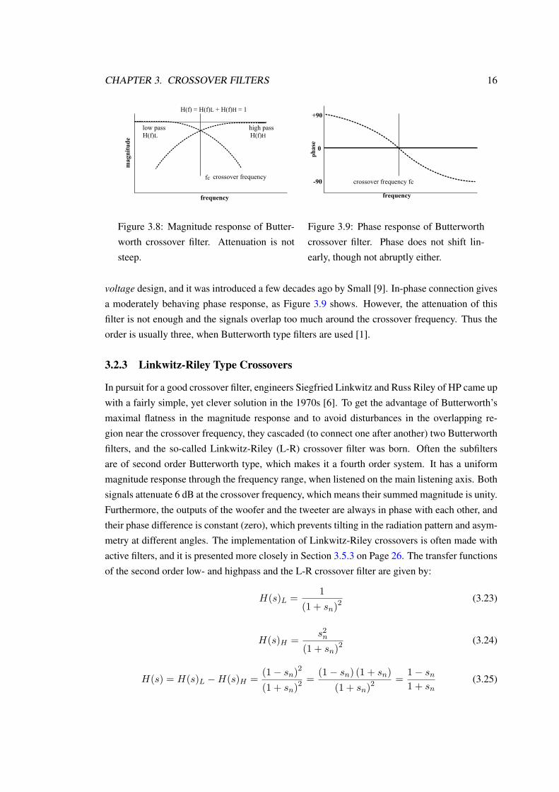
Figure 3.8: Magnitude response of Butter-worth crossover filter. Attenuation is notsteep.
Figure 3.9: Phase response of Butterworthcrossover filter. Phase does not shift lin-early, though not abruptly either.
voltage design, and it was introduced a few decades ago by Small [9]. In-phase connection givesa moderately behaving phase response, as Figure 3.9 shows. However, the attenuation of thisfilter is not enough and the signals overlap too much around the crossover frequency. Thus theorder is usually three, when Butterworth type filters are used [1].
3.2.3 Linkwitz-Riley Type Crossovers
In pursuit for a good crossover filter, engineers Siegfried Linkwitz and Russ Riley of HP came upwith a fairly simple, yet clever solution in the 1970s [6]. To get the advantage of Butterworth’smaximal flatness in the magnitude response and to avoid disturbances in the overlapping re-gion near the crossover frequency, they cascaded (to connect one after another) two Butterworthfilters, and the so-called Linkwitz-Riley (L-R) crossover filter was born. Often the subfiltersare of second order Butterworth type, which makes it a fourth order system. It has a uniformmagnitude response through the frequency range, when listened on the main listening axis. Bothsignals attenuate 6 dB at the crossover frequency, which means their summed magnitude is unity.Furthermore, the outputs of the woofer and the tweeter are always in phase with each other, andtheir phase difference is constant (zero), which prevents tilting in the radiation pattern and asym-metry at different angles. The implementation of Linkwitz-Riley crossovers is often made withactive filters, and it is presented more closely in Section 3.5.3 on Page 26. The transfer functionsof the second order low- and highpass and the L-R crossover filter are given by:
H(s)L =1
(1 + sn)2 (3.23)
H(s)H =s2n
(1 + sn)2 (3.24)
H(s) = H(s)L −H(s)H =(1− sn)2
(1 + sn)2 =(1− sn) (1 + sn)
(1 + sn)2 =1− sn1 + sn
(3.25)
CHAPTER 3. CROSSOVER FILTERS 17
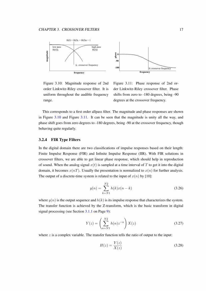
Figure 3.10: Magnitude response of 2ndorder Linkwitz-Riley crossover filter. It isuniform throughout the audible frequencyrange.
Figure 3.11: Phase response of 2nd or-der Linkwitz-Riley crossover filter. Phaseshifts from zero to -180 degrees, being -90degrees at the crossover frequency.
This corresponds to a first order allpass filter. The magnitude and phase responses are shownin Figure 3.10 and Figure 3.11. It can be seen that the magnitude is unity all the way, andphase shift goes from zero degrees to -180 degrees, being -90 at the crossover frequency, thoughbehaving quite regularly.
3.2.4 FIR Type Filters
In the digital domain there are two classifications of impulse responses based on their length:Finite Impulse Response (FIR) and Infinite Impulse Response (IIR). With FIR solutions incrossover filters, we are able to get linear phase response, which should help in reproductionof sound. When the analog signal x(t) is sampled at a time interval of T to get it into the digitaldomain, it becomes x(nT ). Usually the presentation is normalized to x(n) for further analysis.The output of a discrete-time system is related to the input of x(n) by [10]:
y(n) =N2∑
k=N1
h(k)x(n− k) (3.26)
where y(n) is the output sequence and h(k) is its impulse response that characterizes the system.The transfer function is achieved by the Z-transform, which is the basic transform in digitalsignal processing (see Section 3.1.1 on Page 9):
Y (z) =
(N2∑
n=N1
h(n)z−n)X(z) (3.27)
where z is a complex variable. The transfer function tells the ratio of output to the input:
H(z) =Y (z)X(z)
(3.28)

CHAPTER 3. CROSSOVER FILTERS 18
101
102
103
104
-40
-35
-30
-25
-20
-15
-10
-5
0
5Magnitude response of FIR 700
Gai
n [d
B]
Frequency [Hz]
low pass filteredhigh pass filteredsummed signal (output)
0 0.5 1 1.5 2
x 104
-7
-6
-5
-4
-3
-2
-1
0x 10
4 Phase respone of FIR 700
Pha
se [d
eg]
Frequency [Hz]
summed signal (output)
Figure 3.12: Magnitude response of 700thorder FIR crossover filter. Attenuation isreally steep, of ”brick-wall” type.
101
102
103
104
-40
-35
-30
-25
-20
-15
-10
-5
0
5Magnitude response of FIR 700
Gai
n [d
B]
Frequency [Hz]
low pass filteredhigh pass filteredsummed signal (output)
0 0.5 1 1.5 2
x 104
-7
-6
-5
-4
-3
-2
-1
0x 10
4 Phase respone of FIR 700
Pha
se [d
eg]
Frequency [Hz]
summed signal (output)
Figure 3.13: Phase response of 700th orderFIR crossover filter. Phase shifts linearlythroughout the audible frequency range.
hence being able to derive the transfer function of a FIR filter that has an impulse response oflength N2−N1.
H(z) =N2∑
n=N1
h(n)z−n (3.29)
By using the Z-transform signals can be analyzed in the z-domain, which can be particularlyuseful for crossover design. With the possibility of linear phase response, FIR filters can beinteresting as crossover filters. Additionally, the attenuation characteristic can be made arbitrar-ily good by increasing the order, and the term ”brick-wall attenuation” is used for very steepseparation of the audio spectrum. These properties are shown in Figures 3.12 and 3.13. FIRfilters have no feedback property, so they differ fundamentally from analog filters and digital IIRfilters. Linearity in phase response requires symmetry in impulse response.
3.2.5 Goal of Crossover Design
To conclude all these demands for crossover filters and their transfer functions, we end up withthe following goals, as Linkwitz [6], and Lipshitz and Vanderkooy [7] did in their articles:
1. Flatness in the magnitude response. That is, the output signals from woofer and tweetersum up to unity on the main listening axis; there are no dips or peaks at any frequency.
2. Adequately steep cutoff rates of the low- and highpass filters. This is to ensure thatthe drivers operate on their optimal range, and to minimize the interference between thedrivers.
3. Phase difference is zero between the woofer output and the tweeter output at the crossoverfrequency. This prevents tilting in the loudspeaker’s radiation pattern.
CHAPTER 3. CROSSOVER FILTERS 19
4. Ideal polar response of the loudspeaker by having the same phase difference betweenoutputs at all frequencies. That is, the reproduction of the loudspeaker is symmetrical as afunction of angle and it requires the same group delay from low- and highpass filters.
3.3 Passive Crossover Filters
Passive filters have been the most common solution in loudspeakers. Majority of home Hi-Fimulti-way loudspeakers still have passive crossover filters, but, for example, in Public Address(outdoor) reproduction passive filters have not been used because of the high power require-ments. In the recent years, home users have also started using active loudspeakers.
Basic components of a passive filter are resistors, capacitors and inductors. They are placed inan electric circuit in order to acquire the wanted crossover frequency, of which lower componentsof the signal are filtered to the woofer and higher components to the tweeter. Filtering the signaldoes not come for free: it may decrease the quality of the reproduced sound as the filter networkmay add phase shift to the output signal and also distort it.
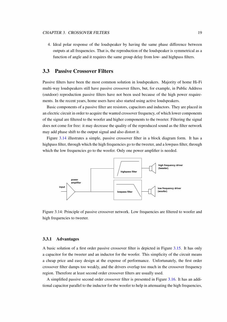
Figure 3.14 illustrates a simple, passive crossover filter in a block diagram form. It has ahighpass filter, through which the high frequencies go to the tweeter, and a lowpass filter, throughwhich the low frequencies go to the woofer. Only one power amplifier is needed.
Figure 3.14: Principle of passive crossover network. Low frequencies are filtered to woofer andhigh frequencies to tweeter.
3.3.1 Advantages
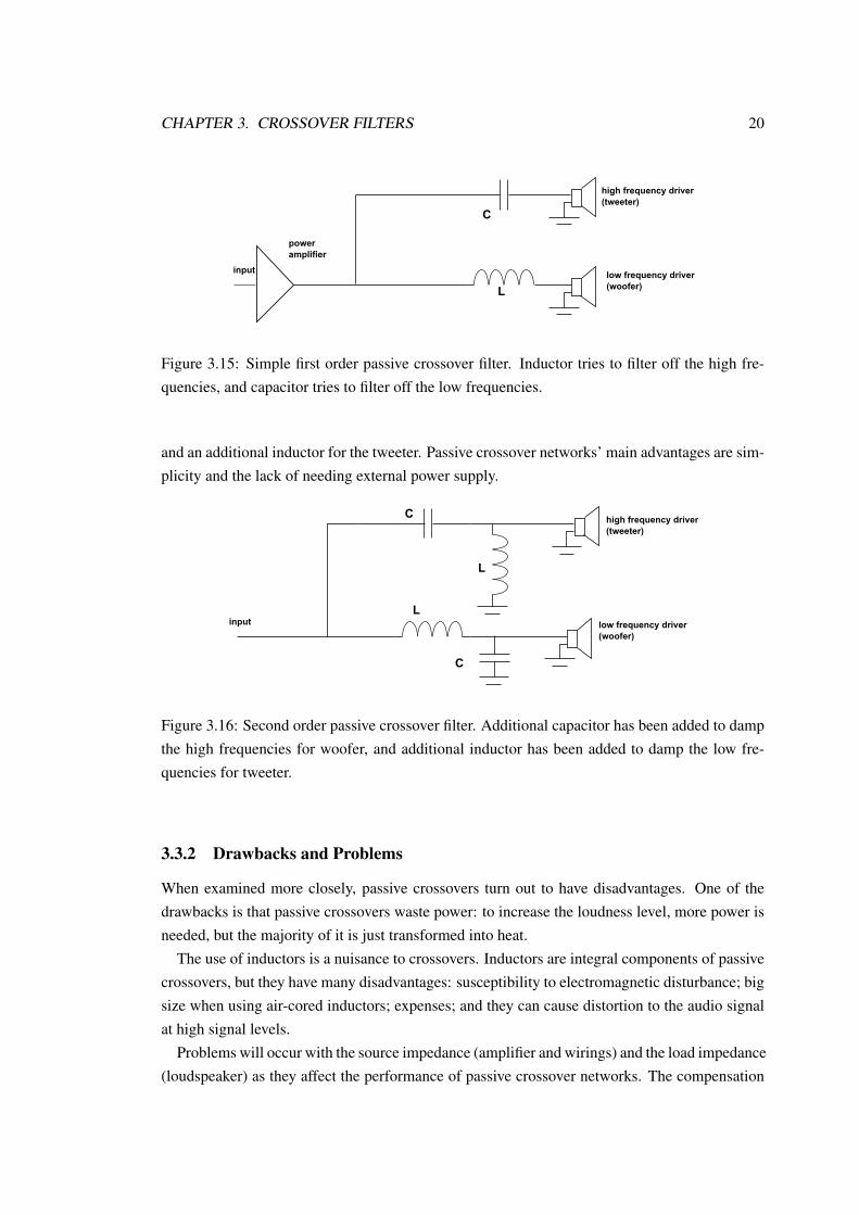
A basic solution of a first order passive crossover filter is depicted in Figure 3.15. It has onlya capacitor for the tweeter and an inductor for the woofer. This simplicity of the circuit meansa cheap price and easy design at the expense of performance. Unfortunately, the first ordercrossover filter damps too weakly, and the drivers overlap too much in the crossover frequencyregion. Therefore at least second order crossover filters are usually used.
A simplified passive second order crossover filter is presented in Figure 3.16. It has an addi-tional capacitor parallel to the inductor for the woofer to help in attenuating the high frequencies,
CHAPTER 3. CROSSOVER FILTERS 20
Figure 3.15: Simple first order passive crossover filter. Inductor tries to filter off the high fre-quencies, and capacitor tries to filter off the low frequencies.
and an additional inductor for the tweeter. Passive crossover networks’ main advantages are sim-plicity and the lack of needing external power supply.
Figure 3.16: Second order passive crossover filter. Additional capacitor has been added to dampthe high frequencies for woofer, and additional inductor has been added to damp the low fre-quencies for tweeter.
3.3.2 Drawbacks and Problems
When examined more closely, passive crossovers turn out to have disadvantages. One of thedrawbacks is that passive crossovers waste power: to increase the loudness level, more power isneeded, but the majority of it is just transformed into heat.
The use of inductors is a nuisance to crossovers. Inductors are integral components of passivecrossovers, but they have many disadvantages: susceptibility to electromagnetic disturbance; bigsize when using air-cored inductors; expenses; and they can cause distortion to the audio signalat high signal levels.
Problems will occur with the source impedance (amplifier and wirings) and the load impedance(loudspeaker) as they affect the performance of passive crossover networks. The compensation

CHAPTER 3. CROSSOVER FILTERS 21
for the inductances of driver’s voice coil can be done by adding a compensation circuit parallelto the driver unit [2]. One solution is called a Zobel network [1], and it has just a resistance anda capacitor in series, which are then connected parallel to the driver. The components’ valuesare calculated directly from the driver’s resistance and inductance values [2].
So called back-EMF (back-electromotive force) may also cause problems. The voice coilkeeps on moving after the signal has stopped coming from the power amplifier, which creates anew voltage due to the electromotive force. The new signal created returns to the network andit can disturb the drivers. The damping factor, df, tells the power amplifier’s ability to damp thereturning signal. It is defined by [1]:
df =Zload
Zsource(3.30)
where Zload is the load impedance and Zsource is the source impedance.Finally, compensating for the impedance variations is not sufficient as the frequency responses
of the drivers may have to be compensated. Therefore magnitude response equalization is com-monly needed as well [2]. Compensating for many things causes that the real implementationsof passive crossovers can become very complicated.
3.4 Active Crossover Filters
Active crossover filters have become increasingly popular recently. Their advantages have beenstudied, and nowadays the professional audio industry uses active filtering in their active monitorspeakers. The fundamental difference of active compared to passive filters is that now the signalis filtered to the drivers before power amplification.
Figure 3.17 shows the principle of an active crossover network. First, filtering is done by theactive low- and highpass filter, and then signals are directed to the power amplifiers and further onto the low- and high-frequency drivers. The active crossover network needs one power amplifierfor each additional driver, and external power for the active filters.
Figure 3.17: Principle of active crossover network. Signals are low- and highpass filtered beforepower amplification.

CHAPTER 3. CROSSOVER FILTERS 22
3.4.1 Advantages and Drawbacks
Active crossovers are superior to their passive counterparts in sound quality if carefully designed.They offer many advantages, such as better power handling, getting rid of inductors, easieradjustability, less (intermodulation) distortion. The biggest advantages of active crossover filtersare that they are separated electrically from the driver and they can operate on low signal andpower levels.
Active crossover filters can be realised without inductors using resistors, capacitors, and am-plifiers called operation amplifiers (op amps). The difference between a lowpass crossover filterrealised passively and actively is presented in Figure 3.18 [2]. The active filter is fed from alow-level source, after which it lowpass filters the signal and then sends it to a specified poweramplifier. Direct connection between the power amplifier and the driver is beneficial for goodcontrol of the driver, as impedance and back-EMF problems decrease. The impedances andsensitivities of the drivers have not to be thought as a whole [6].
Avoiding the use of inductors saves from trouble, but money as well, as large inductors canbe expensive. Additionally, distortion should be smaller in active systems, because there are noinductors causing it at high signal levels.
Figure 3.18: Difference between second order active a) and passive b) crossover filters. Noticethe different order of operations: passive amplifies first and does filtering, active does it viceversa.
Optimizing the operation range of each driver and corresponding power amplifier enableslouder and clearer sound. Intermodulation distortion, which is unwanted interference of soundwaves at different frequencies, is reduced. Time-alignment (see Figure 3.6 on Page 14) of thedrivers may be easier to implement so that the drivers radiate coplanarly. Other equalizationsand adjustments can also be made within the system [2].
The main drawbacks of an active crossover filter can be concluded to be the need of an externalpower supply to the system, as well as the need of additional power amplifiers.

CHAPTER 3. CROSSOVER FILTERS 23
3.4.2 Practical Solutions
The de facto active crossover filter is the Linkwitz-Riley crossover (L-R) [6], whose transferfunction was presented in 3.2.3 on Page 16. The most often used realization of the L-R filteris an active 4th order crossover filter. Its circuit diagram is presented in Figure 3.19. Linkwitzpresented also a passive form in [11].
2R
2R
2C
2C
R R
R
R
C C
C C
RR
input
C
C
to tweeter channel
to woofer channel
Figure 3.19: 4th order Linkwitz-Riley crossover filter.
A crucial assumption for an L-R crossover filter to work properly is that the drivers have beentime-aligned to radiate from the same plane that is also parallel to the loudspeaker cabinet’sfront plane [6]. Otherwise tilting in the radiation pattern will occur in the crossover region(see Figure 3.6 for time-alignment). Having all-pass network characteristics, an L-R filter has afrequency dependent group delay, which may be a problem with higher filter orders. The mainquestions are: is the group delay distortion audible and if yes, how much of it is allowed atdifferent frequencies? Linkwitz referred to the problem already in his celebrated article in 1976,and was of the opinion that generally phase distortion due to the filter is not audible [6, 12].He has also introduced the problem on his web pages [13], but adds nothing essential to theoriginal article. Many other authors have researched the audibility of phase distortion in therecent decades [14, 15, 16, 17, 18, 19, 20, 21, 22]. The conclusions of various tests have beenthat large enough group delay errors may produce audible errors, but when listened to music orsome other real sound material, the differences are often inaudible. More on this topic will bediscussed in Section 4.4.2 on Page 37.
The Linkwitz-Riley crossover alignment has had few seriously taken competitors. One ap-proach is to use different Bessel type filters to build a crossover filter [23]. As listed in Table3.1 on Page 12, Bessel type filters offer the possibility to minimise the changing group delayand thus minimise phase distortion problems, but the trade-off is a non-flat magnitude response.As known that magnitude variations are more audible than phase variations [24], Bessel typefilters are not at the same quality level as the Linkwitz-Riley, as the author in [23], Bohn of
CHAPTER 3. CROSSOVER FILTERS 24
RANE Corporation, notices. A different implementation of the L-R crossover is introduced inChalupa’s article [25] by a subtractive approach. It does not offer much new, just different typeof implementation of the Linkwitz’s design.
As discussed, the audio quality of sound reproduction will most likely be better with activecrossover filters. Also the general opinion has been changing towards it, although passive sys-tems are still widely used. Power amplifier optimization, avoiding lousy, expensive inductors,and adjustability make the active filters a better choice.
3.5 Digital Crossover Filters
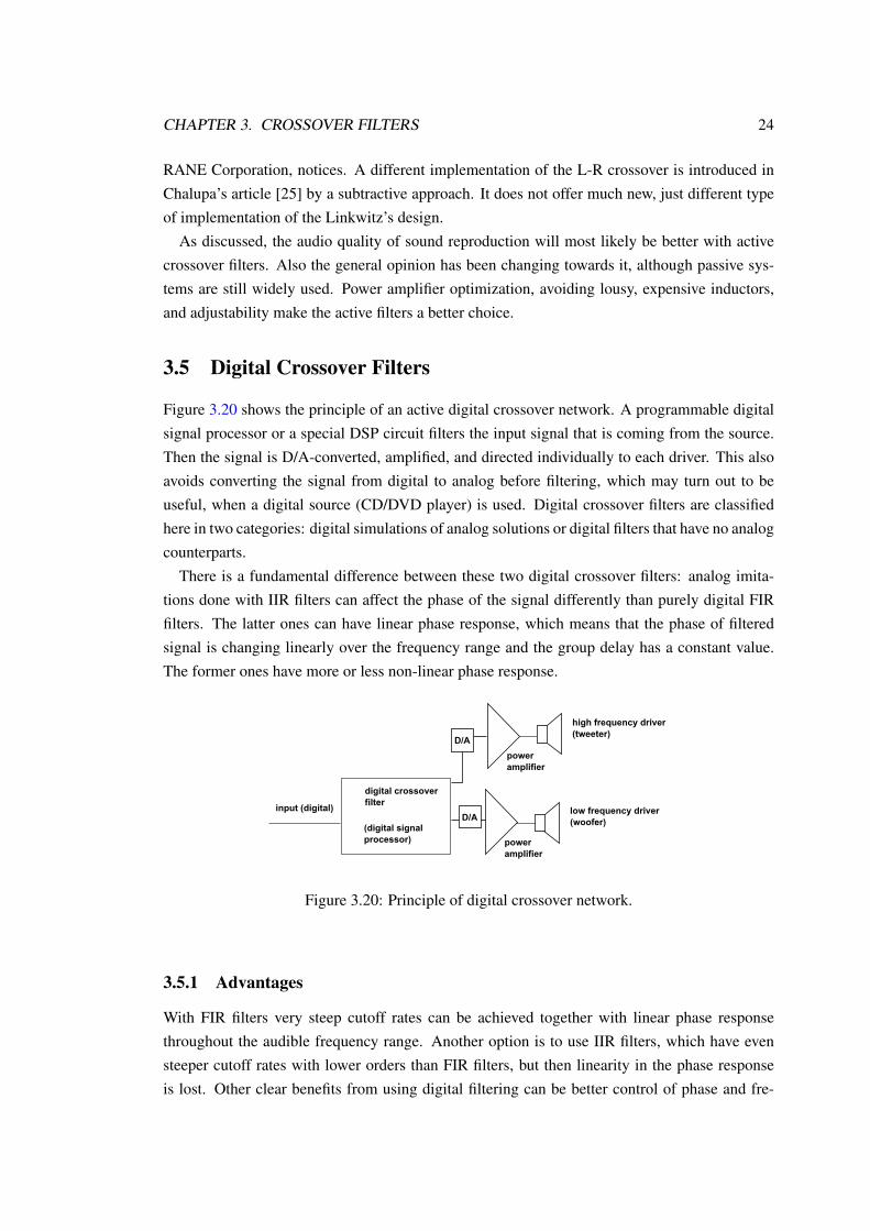
Figure 3.20 shows the principle of an active digital crossover network. A programmable digitalsignal processor or a special DSP circuit filters the input signal that is coming from the source.Then the signal is D/A-converted, amplified, and directed individually to each driver. This alsoavoids converting the signal from digital to analog before filtering, which may turn out to beuseful, when a digital source (CD/DVD player) is used. Digital crossover filters are classifiedhere in two categories: digital simulations of analog solutions or digital filters that have no analogcounterparts.
There is a fundamental difference between these two digital crossover filters: analog imita-tions done with IIR filters can affect the phase of the signal differently than purely digital FIRfilters. The latter ones can have linear phase response, which means that the phase of filteredsignal is changing linearly over the frequency range and the group delay has a constant value.The former ones have more or less non-linear phase response.
Figure 3.20: Principle of digital crossover network.
3.5.1 Advantages
With FIR filters very steep cutoff rates can be achieved together with linear phase responsethroughout the audible frequency range. Another option is to use IIR filters, which have evensteeper cutoff rates with lower orders than FIR filters, but then linearity in the phase responseis lost. Other clear benefits from using digital filtering can be better control of phase and fre-

CHAPTER 3. CROSSOVER FILTERS 25
quency responses including response equalization techniques, better tailoring of filters to matchthe drivers, little intermodulation distortion, easier time delay, better stability of components(no time-or temperature dependence), reduced circuit noise [26], and also a direct interface to aCD/DVD-player in the digital domain.
Some simulations [27] and implementations [28, 26, 29] of digital crossover filters have beenmade, though such de facto crossover filter like the Linkwitz-Riley in the analog world has notyet been introduced.
3.5.2 Drawbacks and Problems
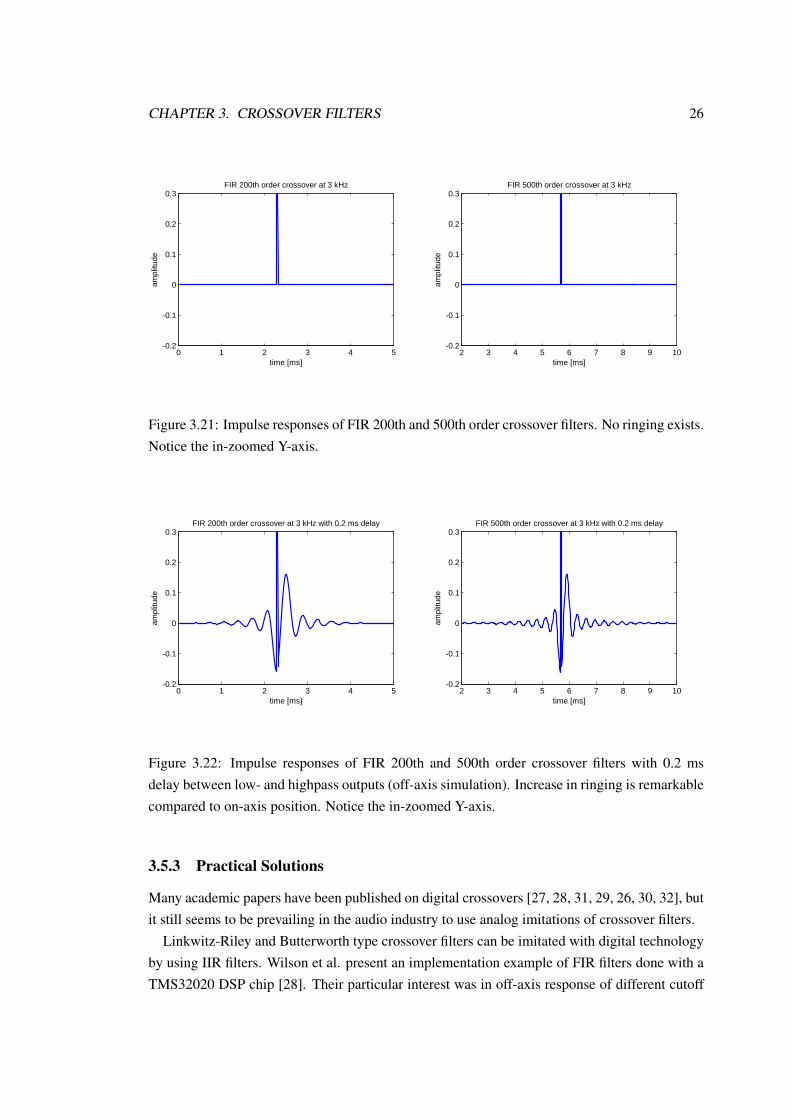
A considerable phenomenon with steep cutoff rates in the FIR case is the ringing of their off-axisresponse [26]. Listening on-axis, the magnitudes of the low- and highpass outputs sum up nicely,and being a linear phase filter, no phase or magnitude problems should occur. However, whenchanging the summing (listening) positions off the axis, the low- and highpass outputs do notsum coherently. Ringing in the impulse response by the Gibbs phenomenon [10] will becomemore audible, increasingly with higher filter orders. The impulse responses of FIR crossoverfilters with orders 200 (left) and 500 (right) at the crossover frequency of 3 kHz are illustratedin closely zoomed Figure 3.21. To illustrate the remarkable growth of the ringing phenomenon,time delay 0.2 ms is added between the low- and highpass outputs of the same crossovers. Figure3.22 depicts this. Looking at the group delay plots when the listening position shifts off the mainaxis, it can also be seen that the group delay is far from a constant. More details on this will begiven in Chapter 5.
There has not been much studies on the audibility of phase distortion and ringing in differentcases. Therefore a listening test was conducted and is reported in Chapter 5.
Rimell and Hawksford came up with the conclusion that it might be better to use lower filterorders in order to avoid ringing, and they introduce a Gaussian filter solution in their article[26]. Greenfield has also paid attention to this problem in his paper [30]. He suggests the use ofpseudo-analog filter functions.
Steeper cutoff means latency (delay) in the systems as the order of a FIR filter is increased(see the block diagram 3.2 on Page 11). This can create problems when sound and picture haveto be synchronized. Only a couple of milliseconds of extra delay can be disturbing in the mostcritical applications. High computational requirements can also be considered as a problem, andthus often different kind of design methods are used to lower the requirements, but possiblysacrifying desired linearity in phase response.
Summing up the problems with increasing filter orders, apparently ”ideal” properties, such as”brick-wall filtering”, on the paper seem not to be immaculate in the reality.
CHAPTER 3. CROSSOVER FILTERS 26
0 1 2 3 4 5-0.2
-0.1
0
0.1
0.2
0.3
time [ms]
ampl
itude
FIR 200th order crossover at 3 kHz
2 3 4 5 6 7 8 9 10-0.2
-0.1
0
0.1
0.2
0.3
time [ms]
ampl
itude
FIR 500th order crossover at 3 kHz
Figure 3.21: Impulse responses of FIR 200th and 500th order crossover filters. No ringing exists.Notice the in-zoomed Y-axis.
0 1 2 3 4 5-0.2
-0.1
0
0.1
0.2
0.3
time [ms]
ampl
itude
FIR 200th order crossover at 3 kHz with 0.2 ms delay
2 3 4 5 6 7 8 9 10-0.2
-0.1
0
0.1
0.2
0.3
time [ms]
ampl
itude
FIR 500th order crossover at 3 kHz with 0.2 ms delay
Figure 3.22: Impulse responses of FIR 200th and 500th order crossover filters with 0.2 msdelay between low- and highpass outputs (off-axis simulation). Increase in ringing is remarkablecompared to on-axis position. Notice the in-zoomed Y-axis.
3.5.3 Practical Solutions
Many academic papers have been published on digital crossovers [27, 28, 31, 29, 26, 30, 32], butit still seems to be prevailing in the audio industry to use analog imitations of crossover filters.
Linkwitz-Riley and Butterworth type crossover filters can be imitated with digital technologyby using IIR filters. Wilson et al. present an implementation example of FIR filters done with aTMS32020 DSP chip [28]. Their particular interest was in off-axis response of different cutoff

CHAPTER 3. CROSSOVER FILTERS 27
rates between filters. After having performed listening tests in a well damped listening room withloudspeakers and with music samples, they concluded that a wider dip in the magnitude responsewas significantly audible, which could be predictable. They suggested already in 1989 that DSPtechnology is usable in crossover filters, though noticing the limitations of DSP technology then.
One of the most interesting applications is presented by Baird and McGrath in 2003 [33].They present a brick-wall type FIR crossover filter with linear phase response. They comparetheir creation with L-R filter with radiation error plots, which are illustrated in Figures 3.23 and3.24. The figures show the magnitude of the error in radiation pattern as a function of angleand frequency. The radiation error is indeed smaller with the linear phase, brick-wall crossover.Presenting a later approach to the subject in a newer article in 2005 [34] with more profoundmeasurements and with real loudspeaker systems, their application is interesting. However,interesting is the lack of perceptual tests, as good plans on the paper do not always go hand inhand with the reality, especially when the off-axis listening problems of digital crossover filtersare known [30].
Figure 3.23: Magnitude of radiation error of linear phase, brick-wall crossover. Adopted from[33]
3.6 Summary of Crossover Filters
Many aspects of loudspeaker crossover filters and their design have been discussed in this chap-ter. Fundamentally, the wide audible frequency range makes it necessary to use a crossover filterin a loudspeaker. The basic classification of a crossover filter is whether the filter is passive or

CHAPTER 3. CROSSOVER FILTERS 28
Figure 3.24: Magnitude of radiation error of L-R crossover. Adopted from [33]
active. Digital crossover filters have also made their entrance into loudspeaker design as thecomputation power has increased. Due to the contribution of both drivers in the crossover fre-quency region, different errors exist. The audibility of these errors has been under discussion fora long time. To find out the reasons why the errors caused by crossover filters can be perceived,an introduction to psychoacoustics is needed. The next chapter will cover the basics of hearing.

Chapter 4
Psychoacoustics
Hearing is one of our five senses. Given the difficulties in physiological measurements and thecomplexity of hearing, its operation is not fully understood. Hearing involves not only our ears,but also a central processing system ending up to the brain.
The physiological and psychophysical aspects of hearing are measured differently. The for-mer is based on the direct measurements from the auditory system, while the latter is measuredsubjectively by different means. The term psychoacoustics basically means representing sub-jective attributes instead of physical attributes. Descriptions given in psychoacoustics can beexpressed in numbers or terms. For example, loudness can be 40 phons; or sound can be saidto be ”warm” or ”metallic”. In Table 4.1 the main physical attributes and their nearest psychoa-coustical correspondences are given [35]. It is emphasized that while the loudness, pitch andsubjective duration are unidimensional, timbre is not [24].
Physical / unit Psychoacoustical /unitPressure / Pascal Loudness / phon
Frequency / Hertz Pitch / mel
Length / s Subjective duration / dura
Spectrum Timbre, not single unit
Table 4.1: Analogues of physical and psychoacoustical attributes. Timbre is the closest corre-spondence to spectrum, though it cannot be physically described by one attribute.
The motivation of this chapter is to make the reader familiar with psychoacoustical attributesas well as with the perception of sound. First, a short introduction to the auditory system is pro-vided. Second, the psychoacoustical attributes of timbre and colouration are explained, becausetimbre is one of the important concepts of the thesis. Third, the spectral and temporal processingof sound are introduced. Finally, a brief inspection of spatial perception of sound is carried out.
29

CHAPTER 4. PSYCHOACOUSTICS 30
4.1 Auditory System
Hearing consists of the ear, neural pathways and the central processing system, which uses alsovisual information to interpret the perception of sound. The ear is divided into three parts: theexternal ear, the middle ear and the inner ear. These parts are illustrated in Figure 4.1, in whichwe can see the basic structure of the ear. The external ear includes the pinna and the ear canal,which are responsible of gathering sound waves and transporting them towards the tympanicmembrane. After the sound waves have arrived at the tympanic membrane, they are conductedfurther by the middle ear, which consists of tiny bones, malleus, incus and stapes. They are usedfor impedance matching between the surrounding air and the fluid in the inner ear. Without themiddle ear, most of the sound would not be transferred into the auditory system, but reflectedaway, as the conduction in the air is very different from conduction in fluid. The transformationthrough the middle ear is most sensitive at the middle frequencies from 500 to 4000 Hz [24].
Figure 4.1: The structure of the ear. Sound waves are captured into the ear canal and onto thetympanic membrane. Malleus, incus and stapes are bones in the middle ear that conduct thewaves into the inner ear. The cochlea is a spiral-shaped organ that analyses the sound. [35]
The inner ear has a specific organ, called the cochlea. Its spiral-type structure is shown in Fig-ure 4.1 and a cut of the cochlea is illustrated in Figure 4.2. There is no evidence of the cochlea’stwisted form being beneficial some way, except saving space [24]. The cochlea is filled withfluid and consists of three chambers, scala vestibuli, scala media and scala tympani, which areseparated by the basilar membrane and the Reissner’s membrane, as shown in Figure 4.2. Thereare sensor cells, called hair cells (inner and outer), on the basilar membrane on the organ of Corti.They are in touch with the tectorial membrane and excited by the basilar membrane’s vibration.The hair cells send the nerve impulses into the auditory pathways that eventually lead to thebrain. A very recent study in October 2007 [36] shows that in addition to the basilar membrane,the tectoral membrane has a stronger influence on the creation of the hearing experience thanthought before. The researchers of Massachusetts Institute of Technology have found a spesific

CHAPTER 4. PSYCHOACOUSTICS 31
longitudinal wave, which proceeds on the tectoral membrane and contributes into formation of asound event by excitating the hair cells.
Figure 4.2: Cut of the cochlea. When the basilar membrane vibrates, hair cells on it are excitedand send nerve impulses into the auditory pathways. [35]
The ear functions as a frequency analyzer. Different locations on the basilar membrane re-spond to different frequencies of the stimulus and so excite hair cells at different locations. Thebase, which is near the oval window, vibrates more by high frequencies and the other end, apex,more by low frequencies. This fact is illustrated in Figure 4.3. The figure shows the response ofthe basilar membrane at different locations to an impulse as a function of time. It is clearly seen,how lower frequencies create excitation farther away than higher frequencies.
Figure 4.3: Response of the basilar membrane to different frequencies. Y-axis is the amplitude,x-axis is time and on the right there are frequencies at different places on the BM. [35]
The central processing system includes auditory pathways from the ears into the brain, in
CHAPTER 4. PSYCHOACOUSTICS 32
which the auditory cortex does the final interpretation. Each auditory nerve contains roughly30000 neurons. Measurements have been made directly from the neurons to show differentresponse to different stimulus. The response threshold for a neuron is lowest at a specific fre-quency. This is called the characteristic frequency of the neuron.
Interestingly, neurons fire impulses also in the absence of a sound stimulus. They are classifiedinto three classes by the rate of spontaneous firing: 61 % having high spontaneous rate of 18-250spikes per second, 23 % having medium rate of 0,5-18 spikes per second and 16 % having lowrate of <0,5 spikes per seconds [24]. Phase locking is a phenomenon that occurs among neurons.The neurons do not necessarily fire at every cycle of the stimulus, but they always fire at thesame phase of that. Time intervals between firings become thus integer multiples of the periodof the stimulating waveform. Phase locking exists only up to 4-5 kHz [24].
The whole perception can also be a combination of auditory and visual systems, as shown inspeech perception by the McGurk effect [37]. Many ”processing units” in the auditory pathwaysfrom the ear into the brain are also inherent. The cochelar nucleus, superior olivary complexand inferior colliculi are all parts of the auditory pathway. The routes of neural impulses arenot straightforward as they cross with each other and the signals are fed into several processingunits.
4.2 Timbre and Colouration
The most fundamental attributes in psychoacoustics are loudness, pitch, subjective duration andtimbre. While the first three of these can be considered as uni-dimensional, timbre cannot be.Placing sounds in order by loudness or pitch can be possible or even easy, while ordering soundsby timbre is not so straightforward. The definition of timbre is given by the American StandardAssociation’s [38] by the following: ”Timbre is that attribute of auditory sensation in terms ofwhich a listener can judge that two sounds similarly presented and having the same loudness,pitch are dissimilar.” An often used term is also tone quality or tone color. Timbre is the attribute,by which we can recognize different instruments, like the violin from the flute, playing the samenote with the same loudness.
4.3 Perception of Spectral Properties
The ear is known for competent spectral analysis it performs. It considers mainly the magnitudeof the signal instead of both the magnitude and phase, as the famous Ohm’s acoustic law from thenineteenth century states [39]. This can be due to the fact that amplitudes contain more relevantinformation for understanding the signals than phase behaviour, because the phase is often ran-domized when listening in a reverberant space. It must be emphasized that temporal processingshould no way be neglected, and hearing performs analysis in both time- and frequency domainsin a complex way.

CHAPTER 4. PSYCHOACOUSTICS 33
4.3.1 Frequency Masking
The masking effect is one of the fundamental phenomena in psychoacoustics. It exists in boththe frequency- and the time-domain. Both effects have specific roles in lossy audio coding, likeMP3’s, where certain parts of the sound signal that are masked by other sounds can be removedwithout a significant decrease in the quality.
Frequency masking is a complicated phenomenon, and it depends on many properties of themasking sound stimulus (a masker). Wideband noise masks differently than narrow band noise,and a sine wave masks differently than a combination of many sinusoids. The spreading ofmasking can be seen in Figure 4.4, where narrow band noise maskers at different center frequen-cies (solid lines) combine with the absolute threshold of hearing (dashed line). The threshold ofhearing a test tone is then the combined line of the dashed and solid lines. Loudness also affectsto the masking effect. When the sound pressure level is held constant at 60 dB, the graphs arequite symmetric, as seen in Figure 4.4. As the sound pressure level increases, the masking effectwidens toward higher frequencies, while it is approximately constant toward lower frequencies.With complex sounds that contain many frequencies, the masking effect is the combination ofeach harmonic of the sound stimulus. In reality, this is often the case.
Figure 4.4: Masking effect of narrow band noise with different center frequencies. The thresholdof a test tone to be heard consists of the absolute threshold (dashed) and the masker lines (solid).Sound pressure level of maskers is held constant at 60 dB. [35]
4.3.2 Critical Band and Frequency Selectivity
Highly related to the masking effect, a crucial property of hearing is the critical band. It canbe considered the frequency domain resolution of hearing with complex sounds. This meansthat within such band, hearing processes partials of complex, wideband sound stimulus as awhole. The physiological basis is the place-dependent analysis of sounds in the cochlea. Whencomparing two noise-like sounds having the same power level, the test sound’s bandwidth canbe widened to a critical point before its loudness starts to exceed that of the reference. Thispoint defines the bandwidth of a critical band. Figure 4.5 shows how the loudness is perceived

CHAPTER 4. PSYCHOACOUSTICS 34
constant as the bandwidth of the stimulus is increased up to 160 Hz. The center frequency of thechannel is 1 kHz and the sound pressure level is held constant at 60 dB. After having passed 160Hz, the loudness is sensed to increase linearly as a function of bandwidth.
The center frequency of a critical band is not constantly located in the spectrum as well as thebandwidth is not constant, but they are formed due to the center or fundamental frequency of thesound stimulus. With sinusoidal sounds, the frequency resolution is much better than the criticalband, being a twenty-fifth part of that for a complex sound [35].
Hearing can be thought to process sound as a filterbank of bandpass filters. The shape of thefilters is not rectangular, but more like with a sharp top and sloping edges on both sides. In psy-choacoustics, the scale of frequency resolution is represented either in Bark or ERB (EquivalentRectangular Bandwidth) scale. One critical band corresponds a Bark band, and ERB tries tomodel the bandwidth of auditory analysis. A suggestion based on physiological measurementsis to use the ERB scale. The bandwidth of an ERB band is typically from 11 to 17 % of thecenter frequency. The corresponding ERB band ERBn in Hz as a function of center frequencyF in kHz is given by [24]
ERBn = 24.7(4.37F + 1) (4.1)
Figure 4.5: Definition of critical bandwidth at the center frequency of 1 kHz. Loudness isperceived as a constant up to bandwidth of 160 Hz, after which it increases linearly. [35]
Separation of partial tones from a complex stimulus is an impressive specimen of hearing’sskill. Plomp [40, 41] has found that the ear is able to hear out 5-7 individual partials in complex,periodic sound. However, the tests showed that the partials could only be heard out if they wereseparated by more than a critical bandwidth. This seems to be in harmony with the critical bandtheory. Plomp himself doubted the consistency at low frequencies, but B.C.J. Moore states in”An Introduction to the Psychology of Hearing” that a better consistency to the separation ofa partial from its neighbour is found if the partials are separated by more than 1.25 times theERB-bandwidth [24].

CHAPTER 4. PSYCHOACOUSTICS 35
4.3.3 Frequency Sensitivity and Loudness
Hearing processes sound non-linearly. One of the examples is the equal loudness contours,originally presented by Fletcher and Munson [42]. Figure 4.6 shows the subjective loudness inphons for sound pressure level in decibels. The reference point is defined so that the subjectiveloudness at 1 kHz equals the sound pressure level at 1 kHz. As seen, loudness level of 40 phonsrequires a sound pressure level of 40 dB at 1 kHz, whereas it requires almost 90 dB to producethe same perceived loudness at 20 Hz. The ear is less sensitive outside the mid-frequencies,roughly below 500 and above 4000 Hz.
Figure 4.6: Equal loudness contours for a sinusoidal sound. The absolute hearing threshold isthe dashed line, and subjective loudness is presented as curves so that loudness in phons at 1 kHzequals sound pressure level at 1 kHz. [35]
Loudness depends also on the bandwidth of the stimulus. On the whole, wideband noise isperceived more loud than a sinusoid. It could already be seen in Figure 4.5, where the loudnessis increasing as the bandwidth exceeds the critical bandwidth. An important property of hearingis the just noticeable difference (JND) of change in loudness. JND is roughly 1 dB on moderatesound pressure levels, but it changes towards higher or lower sound pressure levels. This im-portant fact is illustrated in Figure 4.7 for a sinusoid and for white noise. The test is conductedwith a 4 Hz amplitude-modulated sinusoid. Modulation by 4 Hz tone is known to be the mostsensitive to perceive.
The sensation of loudness takes time to build up. The ear integrates sound over a longer period,and this is called ”temporal integration”. The time period over which the loudness sensation isintegrated, is about 200 ms. After it, the sensation of loudness does not change anymore.

CHAPTER 4. PSYCHOACOUSTICS 36
Figure 4.7: Just noticeable difference of amplitude modulation. 1 kHz sinusoid is modulatedwith 4 Hz sinusoid. The solid line tells how much the difference in level must be to perceive themodulation. For moderate sound pressure levels the JND is roughly 1 dB. [35]
4.4 Perception of Temporal Properties
4.4.1 Temporal Masking
Another side of the masking effect encounters in the time domain. Time masking can be dividedinto backward and forward masking. It means that the masking effect begins before the actualmasking tone begins (backward masking) and does not end immediately after the masker hasended (forward masking), as Figure 4.8 illustrates. The solid line shows the threshold level ofa test tone, when a masker lasting at least 200 ms is applied. Remarkably, the masker curve isnot symmetrical, but backward masking exists only about 10 ms before the masker tone, whileforward masking lasts for about 100-200 ms after the masker tone has ended. However, this isthe case only for long maskers. For an impulse type of masker, the masking curve in the timedomain is much more symmetric, as Figure 4.9 illustrates.
Figure 4.8: Masking effect in the time domain for long maskers. The solid line shows thethreshold of test tone for a long masker (at least 200 ms). The masking effect begins 10-20 msbefore the masker is applied and lasts about 100-200 ms after the masker has stopped. Noticethe asymmetry of the masking curve. [35]

CHAPTER 4. PSYCHOACOUSTICS 37
Figure 4.9: Masking effect in the time domain for impulse type maskers that mask impulse typetest signals. Notice that the masking curve is now much more symmetric than for long lastingmaskers. [35]
4.4.2 Perception of Timbre
Recognition of auditory objects by timbre is a complex subject. The main contributors to timbreof a sound are the relations in the amplitudes and phases of the signals. The general acceptanceis that timbre is mainly related to the excitation level in each critical band [43], but temporalchanges cannot be neglected either. The relative phases of signal components can actually havean influence on tone quality. This can be still considered a somewhat controversial topic after acouple of hundred years after Ohm’s statement that the ear is phase deaf. Much research is doneon the effect of relative phase of complex sound’s components on timbre by Pattersons, [44, 45],as well as Plomp and Steeneken [46]. These researches support the importance of phase ontimbre. The temporal resolution of ear was discovered to be approximately 2.5 ms for signalshaving identical energy spectra and differenting only by phase. This experiment was done byPatterson and Green in 1970 [44].
Another factor in recognizing different timbres is the temporal envelope of a signal. A clas-sical example of the importance of the temporal envelope is a piano tone reversed in time. Withhaving the same magnitude spectrum, the reversed piano tone sounds completely different. Pat-terson has obtained results regarding the temporal envelope importance in timbre perception byamplitude modulated, asymmetric envelopes [47]. The results show that time-reversed soundshaving the same long-term magnitude spectrum as originals were heard as either one sound oras two different sounds. This concludes that the timbre definitely depends on more factors thanjust the relative magnitudes of the components.
Recognizing different auditory objects, like musical instruments, is based on many factors.Schouten has defined the recognition of an ”auditory object” to depend on the following factors[48]:
1. Sound periodicity in the range from 20 to 20000 Hz vs. noise-like, irregular sound

CHAPTER 4. PSYCHOACOUSTICS 38
2. Waveform is constant vs. waveform fluctuates as a function of time; fluctuations are simi-lar/dissimilar
3. Other aspect of sound, like spetrum or periodicity is changing as a function of time
4. What are the preceeding and the following sounds like?
From the audio engineer’s point of view, group delay distortions have been used as a measureof phase errors for a long time. The most comprehensive paper on the group delay matters inthe audio field is probably the paper by Lipshitz, Pocock and Vanderkooy [14], supported by[15, 16, 17, 18, 19, 20, 21, 22]. Hoshino and Takegahara [49] have defined the permissiblevalues for group delay at high frequencies to be roughly 2 ms from 10 kHz, though this has moreimportance in general audio processing than in crossover design, because usually the crossoverfrequencies are way below 10 kHz. A recent study defines the audible value of group delay tobe 1.6 ms [22]. Møller et al. describe the group delay errors as ”ringing” or ”pitchiness” andimportantly state that ”the ringing is detected in the individual ear and not as part of binauralprocessing”.
4.5 Perception of Spatial Properties
Localization of sound events has developed to direct the attention of humans. Localization meansjudging the direction and distance of a sound event, and though possible, it would be way moredifficult without two ears. There are differences in signals arriving at the ears, and the conceptsof inter-aural time difference (ITD) and inter-aural level difference (ILD) between the ears areof the greatest importance. Localization is a learnt property, because it varies among humans asthe shape of the head, the pinnae and the upper body are individual. In headphone listening, thecues for sound localization are lacking, and then hearing often places the sound source insidethe head. This phenomenon is called lateralization. It can cause listening fatigue and annoyance[50]. Interestingly, even though the phenomenon has been in general knowledge for decades, stillno universal solution how to externalize the sound source outside the head has been introduced.
Due to the laws of physics, ITD is the major factor at low frequencies to help in localizationbecause of the relative wavelength of the sound waves are long compared to head’s dimensions.The opposite is true for higher frequencies, as the wavelength is small in relation to head’s di-mensions, and ILD becomes the main reason for localization. Head-related Transfer Functions(HRTF) are used for determining the transfer function from a sound source to the ear in ane-choic conditions. To illustrate the meaning of ILD as a function of arrival angle of sound, themagnitude response is plotted for different angles in Figure 4.10. It can be seen that the higherfrequencies drop in magnitue when the angle is increased, while the lower frequencies exhibita smaller drop. In general, the direction of a sound source is much better localized than thedistance of a sound source.
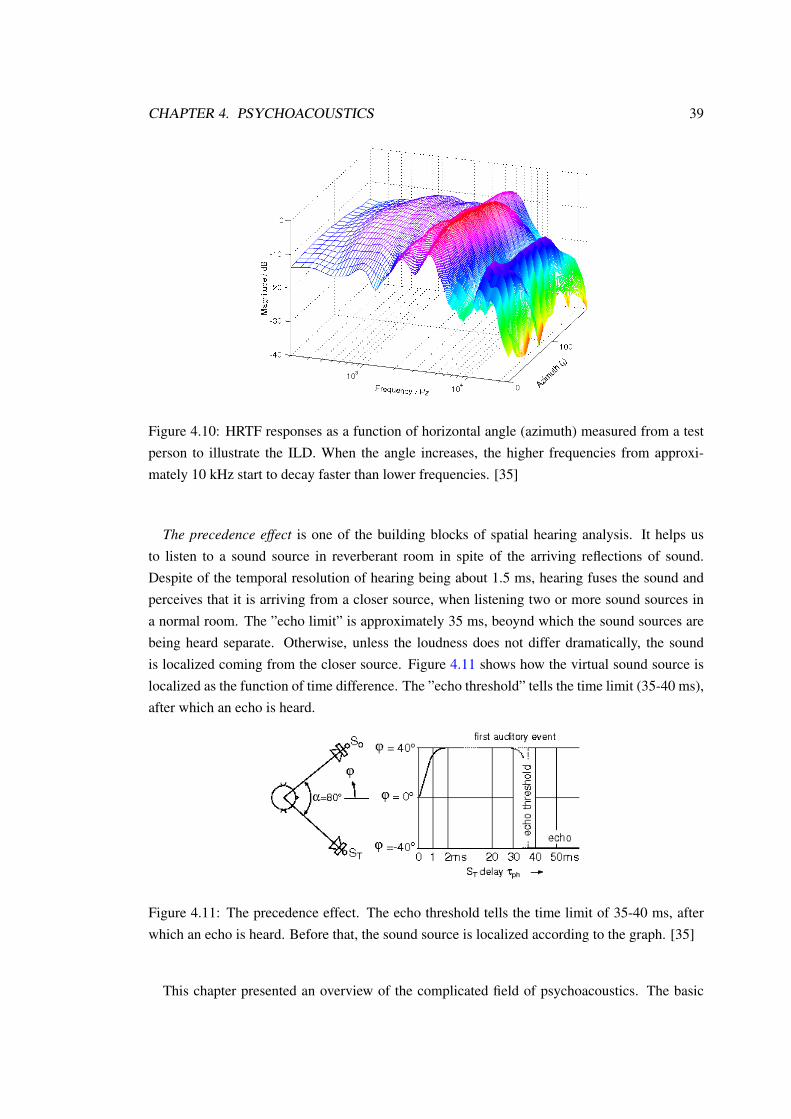
CHAPTER 4. PSYCHOACOUSTICS 39
Figure 4.10: HRTF responses as a function of horizontal angle (azimuth) measured from a testperson to illustrate the ILD. When the angle increases, the higher frequencies from approxi-mately 10 kHz start to decay faster than lower frequencies. [35]
The precedence effect is one of the building blocks of spatial hearing analysis. It helps usto listen to a sound source in reverberant room in spite of the arriving reflections of sound.Despite of the temporal resolution of hearing being about 1.5 ms, hearing fuses the sound andperceives that it is arriving from a closer source, when listening two or more sound sources ina normal room. The ”echo limit” is approximately 35 ms, beoynd which the sound sources arebeing heard separate. Otherwise, unless the loudness does not differ dramatically, the soundis localized coming from the closer source. Figure 4.11 shows how the virtual sound source islocalized as the function of time difference. The ”echo threshold” tells the time limit (35-40 ms),after which an echo is heard.
Figure 4.11: The precedence effect. The echo threshold tells the time limit of 35-40 ms, afterwhich an echo is heard. Before that, the sound source is localized according to the graph. [35]
This chapter presented an overview of the complicated field of psychoacoustics. The basic

CHAPTER 4. PSYCHOACOUSTICS 40
concepts of sound perception were introduced. Timbre, the sound quality, and its perception wasslightly emphasized because of its significance to the perceptual tests carried out in this thesis.For the same reason the spatial perception of sound was left to less attention. The main difficultyin psychoacoustics is to make universal tests and measures to investigate sound phenomena notonly subjectively, but also objectively.
Chapter 5
Listening Experiment
5.1 Motivation and Goals
Careful designs on paper do not always cohere with the perceived reality, and that is why per-ceptual studies are needed. Considering digital crossover filter design for loudspeakers, lack ofperceptual tests is a fact. An experimental study was planned and arranged to help to fix thisshortage. Special interest was laid on the purely digital FIR crossover filter with linear phasecharacteristics and brick-wall attenuation. This way, an ”ideal” crossover filter is approached,though suffering from the ringing phenomenon (see Section 3.5.2 on Page 25 and [30, 22]). An-other crossover filter under study was a digital implementation of the Linkwitz-Riley crossover.It has a uniform magnitude response on-axis and good off-axis response, but as the order in-creases, the peak group delay and the deviation from a uniform group delay grows.
The goals of the study can be set by the following:
1. How much group delay deviations from uniform group delay are allowed for differentsignals, i.e., what is the Just Noticeable Difference (JND limit)? How the type of thegroup delay error affects the audibility?
2. How sensitive are digital crossover filters for off-axis response errors?
3. Is it possible to predict the results of the listening test by objective measures?
5.2 Description of Listening Test
5.2.1 Test Procedure
The experiment was conducted as a comparison test between the original, unprocessed soundsample, and the crossover-simulated sound sample. Simulation with headphones was chosenas the primary test method to reveal small degradations, but also a more brief listening testwas conducted with a real loudspeaker in a listening room to compare the results. Because the
41

CHAPTER 5. LISTENING EXPERIMENT 42
loudspeaker test was different from the simulation experiment, it is discussed in its own Section5.5, starting from Page 58.
Untrained subjects listened to the comparison samples in random order, using a graphicaluser interface (GUI) to respond, and they were supposed to give grades for the basic audioquality difference between the unprocessed and the crossover filtered samples. A screen shot ofthe Matlab [51] GUI is presented in Appendix A. The equipment and instructions given to thesubjects are also presented in the same Appendix A. Oral introduction to the topic, instructions,and guidance were given before the test.
Grading was based on Table 5.1 of ITU’s small impairment scale [52], which is used forjudging small distortions in audio signals. The grade of 5 presents the imperceptible differencein the sample, and the grade of 1 presents high disturbances in the audio quality. The scale isguided to be used at intervals of 0.1, but due to feedback received from preliminary tests, it wasinstead used at intervals of 0.5. Comprehensive training would have been necessary for usingsteps of 0.1. The only trained subject for this test was the author due to preliminary listening ofdifferent scenarios. As the samples were graded in randomized order using the GUI in Matlab,the author could participate to the test. An interesting point is the effect of training, though it isknown to help to detect the group delay distortions [15].
Impairment GradeImperceptible 5.0
Perceptible, but not annoying 4.0
Slightly annoying 3.0
Annoying 2.0
Very annoying 1.0
Table 5.1: The ITU small impairment scale. Grade 5 presents the imperceptible impairment, and1 presents bad disturbance in the signal. The scale was used at intervals of 0.5 in the listeningtest.
5.2.2 Test Material and Parameters
The test material consisted of three different sound samples:
1. 10 Hz square wave
2. The castanets
3. The tom-tom drum
The selection of test material was based on preliminary tests of the topic as well as generalknowledge of psychoacoustics. The square wave is known to be extremely revealing for distor-tions in the audio systems due to its waveform and its contents of odd harmonics. It has also

CHAPTER 5. LISTENING EXPERIMENT 43
been used in many perceptual studies, such as in [16, 14]. The castanets (taken from the AES’audio codec CD) were chosen as a test sound because of its transient nature. The castanet per-cussions are concentrated in a short period of time, and so the phase distortions would affectthe final waveform in an audible way. The third sample was the tom-tom drum (recorder by anindividual, taken from an audio database). It has also a slight impulse nature in its waveform,but not as concentrated as the castanets. It was an interesting sample, because the drum is a verycommon musical instrument, and in contrast to the castanets, it has low frequency contents. Thewaveforms of the three samples are presented in Figure 5.1 to illustrate the described properties.
0 50 100 150 200 250 300 350 400 450 500-1
-0.5
0
0.5
1
time [ms]
ampl
itude
square wave 10 Hz
350 400 450 500 550 600 650-0.5
0
0.5
time [ms]
ampl
itude
castanets
0 100 200 300 400 500 600-1
-0.5
0
0.5
1
time [ms]
ampl
itude
tom-tom
Figure 5.1: Waveforms of the input signals: Square wave (top), castanets (middle), and tom-tom(bottom).
Defining the parameters for simulated crossover filters was planned as carefully as possible.The crossover frequency, at which the audio spectrum is divided into low- and highpass bands,was chosen to be at either 100/300 Hz, 1 kHz or 3 kHz to follow the common divisions in multi-way loudspeakers. The orders of the crossover filters were chosen to be realistic for practicalimplementation, and not to exceed 32 for L-R or 2000 for FIR crossovers. Some exceptionswere included. The delay between low- and highpass outputs was implemented to simulate theelevation of the listening angle, because most of the problems exist, when the vertical angleis changed. With quite a normal separation of drivers of a two-way loudspeaker (0.25 m), thedelay was limited to 0-0.5 ms to simulate far-field elevation angles between 0 and 45 degrees.The parameters have been gathered in Table 5.2 to conclude the diversity of possible scenarios.The large number of different scenarios forced to cut out inaudible (to the author at least) samplesto make the test reasonable in size and duration. For the same reason, the parameters were notalways the same for different signals.
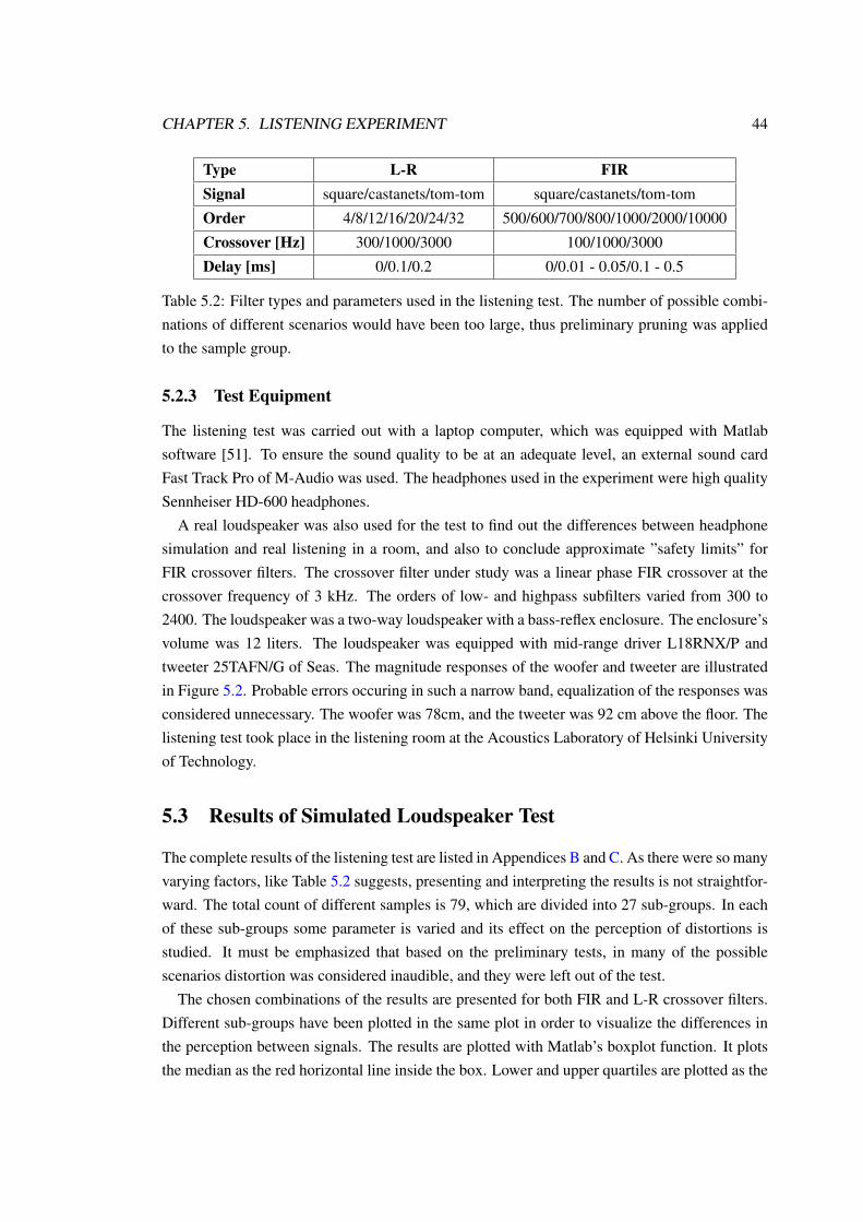
CHAPTER 5. LISTENING EXPERIMENT 44
Type L-R FIRSignal square/castanets/tom-tom square/castanets/tom-tom
Order 4/8/12/16/20/24/32 500/600/700/800/1000/2000/10000
Crossover [Hz] 300/1000/3000 100/1000/3000
Delay [ms] 0/0.1/0.2 0/0.01 - 0.05/0.1 - 0.5
Table 5.2: Filter types and parameters used in the listening test. The number of possible combi-nations of different scenarios would have been too large, thus preliminary pruning was appliedto the sample group.
5.2.3 Test Equipment
The listening test was carried out with a laptop computer, which was equipped with Matlabsoftware [51]. To ensure the sound quality to be at an adequate level, an external sound cardFast Track Pro of M-Audio was used. The headphones used in the experiment were high qualitySennheiser HD-600 headphones.
A real loudspeaker was also used for the test to find out the differences between headphonesimulation and real listening in a room, and also to conclude approximate ”safety limits” forFIR crossover filters. The crossover filter under study was a linear phase FIR crossover at thecrossover frequency of 3 kHz. The orders of low- and highpass subfilters varied from 300 to2400. The loudspeaker was a two-way loudspeaker with a bass-reflex enclosure. The enclosure’svolume was 12 liters. The loudspeaker was equipped with mid-range driver L18RNX/P andtweeter 25TAFN/G of Seas. The magnitude responses of the woofer and tweeter are illustratedin Figure 5.2. Probable errors occuring in such a narrow band, equalization of the responses wasconsidered unnecessary. The woofer was 78cm, and the tweeter was 92 cm above the floor. Thelistening test took place in the listening room at the Acoustics Laboratory of Helsinki Universityof Technology.
5.3 Results of Simulated Loudspeaker Test
The complete results of the listening test are listed in Appendices B and C. As there were so manyvarying factors, like Table 5.2 suggests, presenting and interpreting the results is not straightfor-ward. The total count of different samples is 79, which are divided into 27 sub-groups. In eachof these sub-groups some parameter is varied and its effect on the perception of distortions isstudied. It must be emphasized that based on the preliminary tests, in many of the possiblescenarios distortion was considered inaudible, and they were left out of the test.
The chosen combinations of the results are presented for both FIR and L-R crossover filters.Different sub-groups have been plotted in the same plot in order to visualize the differences inthe perception between signals. The results are plotted with Matlab’s boxplot function. It plotsthe median as the red horizontal line inside the box. Lower and upper quartiles are plotted as the

CHAPTER 5. LISTENING EXPERIMENT 45
102
103
104
-20
-15
-10
-5
0
Magnitude responses of loudspeaker driversG
ain
[dB
]
Frequency [Hz]
woofertweeter
Figure 5.2: Magnitude responses of drivers of the loudspeaker that was used in the real loud-speaker experiment.
bottom and top line of the box. ”Whiskers”, the dashed lines, extend from the ends of the box tothe adjacent values of the data, to the maximum of 1.5 times the interquartile range. The gradesnot in the range of 1.5 times the interquartile are plotted as outliers with an ”x”.
5.3.1 Results of FIR Crossover Filters
The results of 1000th to 2000th order FIR crossovers at 1 kHz are plotted in Figure 5.3. It canbe seen that a 0.2 ms delay between drivers causes clearly perceivable distortion in the squarewave. With a 2000th order FIR at 1 kHz, castanets are susceptible to distortions rather easily,and 0.3 ms delay between the low- and highpass bands produces a perceivable distortion. Thetom-tom drum being the most insusceptible signal, it does not suffer from distortion even with0.5 ms delay at 1 kHz.
0 0,1 0,2 0,3 0,51
2
3
4
5
Gra
de
Delay [ms]
FIR 1000th order crossover at 1 kHz, square wave
0,1/cast 0,2/cast 0,3/cast 0,5/tom1
2
3
4
5
Gra
de
Delay [ms]
FIR 2000th order crossover at 1 kHz, castanets and tom-tom
Figure 5.3: Combined results of the listening test for FIR crossovers at 1 kHz. Square wave issusceptible to clearly audible degradation with 0.2 ms delay, castanets with 0.3 ms delay, whiletom-tom receives high grade even with 0.5 ms delay.
Results for the two other crossover frequencies 100 Hz and 3 kHz are plotted in Figure 5.4.Excluding a couple of outlying grades, the results of FIR crossovers at 100 Hz tell that even

CHAPTER 5. LISTENING EXPERIMENT 46
quite high orders do not produce audible distortions in any of the signals with the maximal delaybetween drivers (0.5 ms). This is illustrated in the top subplot of Figure 5.4.
On the contrary, differences become clearly audible at 3 kHz. The results of FIR crossover at3 kHz with the maximum delay 0.5 ms are presented in the middle subfigure of Figure 5.4. Asthe order of the crossover filter is varied, it seems that castanets begin to suffer from distortionssomewhere between orders of 700 and 1000. The tom-tom presents clearly audible distortionsat order of 700.
When testing the highest order of 2000 with FIR crossovers, interesting results occur, as thebottom subfigure of Figure 5.4 shows. After the smallest delay of 0.01 ms, all the signals startto present audible distortions. The delay is really small, but still the medians of the results areclearly in the disturbance range (below or at the grade of 4). These results will be interesting,because this type of FIR crossover should offer the ”ideal” frequency domain characteristics of acrossover with very high stopband attenuation and yet linearity in the phase response, but as theaudio spectrum is divided steeply in low- and highpass bands, ringing in the time domain occursbecause of the Gibbs phenomenon [10].
5.3.2 Results of Linkwitz-Riley Crossover Filters
A digital implemenation of L-R crossover was simulated to study the audibility of phase distor-tion. The L-R crossover should offer a magnitude response of unity on the listening axis, butit suffers from phase distortion due to increasing group delay deviations as the order increases.Combined results of the Linkwitz-Riley implementations are presented in Figure 5.5. When thecrossover frequency is at 300 Hz, the square wave presents more audible errors than the castanetsor the tom-tom, like the top subplot of Figure 5.5 shows. Looking at the L-R crossover with anorder of 16, the square wave results have received a median grade under 2, while the castanetsand the tom-tom have median grades above 4.
At 1 kHz, the square wave once again suffers from distortion above the order of 8, whereasthe castanets have received acceptable median grade up to order of 16 and the tom-tom does notseem to present considerable distortion up to order of 24. The results of the L-R listening test at1 kHz for all the signals are plotted in the middle subplot of Figure 5.5.
With crossover frequency at 3 kHz, very high orders seem to be acceptable in the light of theresults. With the 10 Hz square wave, orders up to 20, and with the castanets and the tom-tom upto 32, the median grades are clearly above 4.
5.4 Analysis
The reasons for audible reproduction errors can be of two natures. The perceived difference inthe audio quality is caused either by magnitude and/or phase error. A usual measure for phaseerrors is the deviation of the group delay from a constant value. The analysis concentrates onthe computable measures of magnitude error and group delay error. A deeper auditory analysis

CHAPTER 5. LISTENING EXPERIMENT 47
2000/sq 10000/sq 700/cast 10000/cast 700/tom 10000/tom1
2
3
4
5G
rade
Order
FIR crossover at 100 Hz with 0,5 ms delay, all the signals
700/cast 1000/cast 2000/cast 600/tom 700/tom 800/tom 1000/tom 2000/tom1
2
3
4
5
Gra
de
Order
FIR crossover at 3 kHz with 0,5 ms delay, castanets and tom-tom
0,01/sq 0,02/sq 0,03/sq 0,05/sq 0,03/cast 0,05/cast 0,07/cast 0,01/tom 0,03/tom 0,05/tom 0,1/tom1
2
3
4
5
Gra
de
Delay [ms]
FIR 2000th order crossover at 3 kHz, all the signals
Figure 5.4: Combined results of the listening test for FIR crossovers. Top: At 100 Hz no consid-erable degradations are perceived. Middle: At 3 kHz with long delay the grades seem to decreaseafter order of 600-700. Bottom: At 3 kHz with varying delay, even small delays seem to degradethe signals in an audible way.
is documentated in Chapter 6. In order to make the magnitude errors interpretable in termsof psychoacoustics, a smoothed third-octave spectrum was calculated in Matlab. It is a roughmeasure of resolution of the bandpass filterbank of hearing.
Regarding magnitude errors, a general rule of JND is about 1 dB deviation, if the soundpressure level is moderate and there is a comparable reference in the short term memory (seeFigure 4.7 on Page 36). In the crossover filter case, magnitude response should be uniformon-axis. L-R crossovers are known for their relatively good off-axis response, whereas FIRcrossovers are known to suffer from off-axis errors [30]. In the experiment, L-R crossoverswere tested both on- and off-axis. FIR crossovers were tested only off-axis, because the on-axisresponse should be nearly perfect independent of the crossover frequency and the filter order dueto the ”ideal” characteristics of an FIR type crossover filter.
Regarding phase errors, L-R crossovers suffer from increasing group delay at the crossoverfrequency as the order increases. It is interesting to have a clue how much group delay deviationfrom a constant value is allowed for different signals. Do they follow the rule of thumb, which

CHAPTER 5. LISTENING EXPERIMENT 48
8/sq 12/sq 16/sq 4/cast 16/cast 4/tom 16/tom1
2
3
4
5G
rade
Order
L-R crossover at 300 Hz, all the signals
8/sq 24/sq 4/cast 16/cast 24/cast 4/tom 16/tom 24/tom1
2
3
4
5
Gra
de
Order
L-R crossover at 1 kHz, all the signals
20/sq 32/sq 4/cast 16/cast 32/cast 4/tom 16/tom 32/tom1
2
3
4
5
Gra
de
Order
L-R crossover at 3 kHz, all the signals
Figure 5.5: Combined results of the listening test for L-R crossovers. Top: At 300 Hz, only thesquare wave seems to be degraded audibly, while the castanets and the tom-tom have quite highgrades. Middle: At 1 kHz, the square wave suffers from degradation above the order of 8, thecastanets above the order of 16 and the tom-tom does not present clear distortion even at theorder of 24. Bottom: At 3 kHz, degradations become audible with the square wave above theorder of 20, but the castanets and the tom-tom do not suffer from considerable distortions up toorder of 32.
is 1.6 ms [22]? FIR crossovers have a linear phase response through the pass band, which meansa constant group delay. However, when the low- and highpass outputs do not sum up nicely off-axis, errors will also occur for FIR crossovers. Interesting is the shape of the group delay curve.L-R’s group delay rises up as approaching the crossover frequency and then falls toward zeroafterward. Off-axis, FIR provides a constant group delay up to the crossover frequency and afterit, but between the low- and highpass bands, a sudden change occurs. A comparison between8th order L-R at 1 kHz and 1000th order FIR at 1 kHz with 0.2 ms delay is presented in Figure5.6. The group delay of the L-R crossover behaves relatively smoothly if compared to that of theFIR crossover.
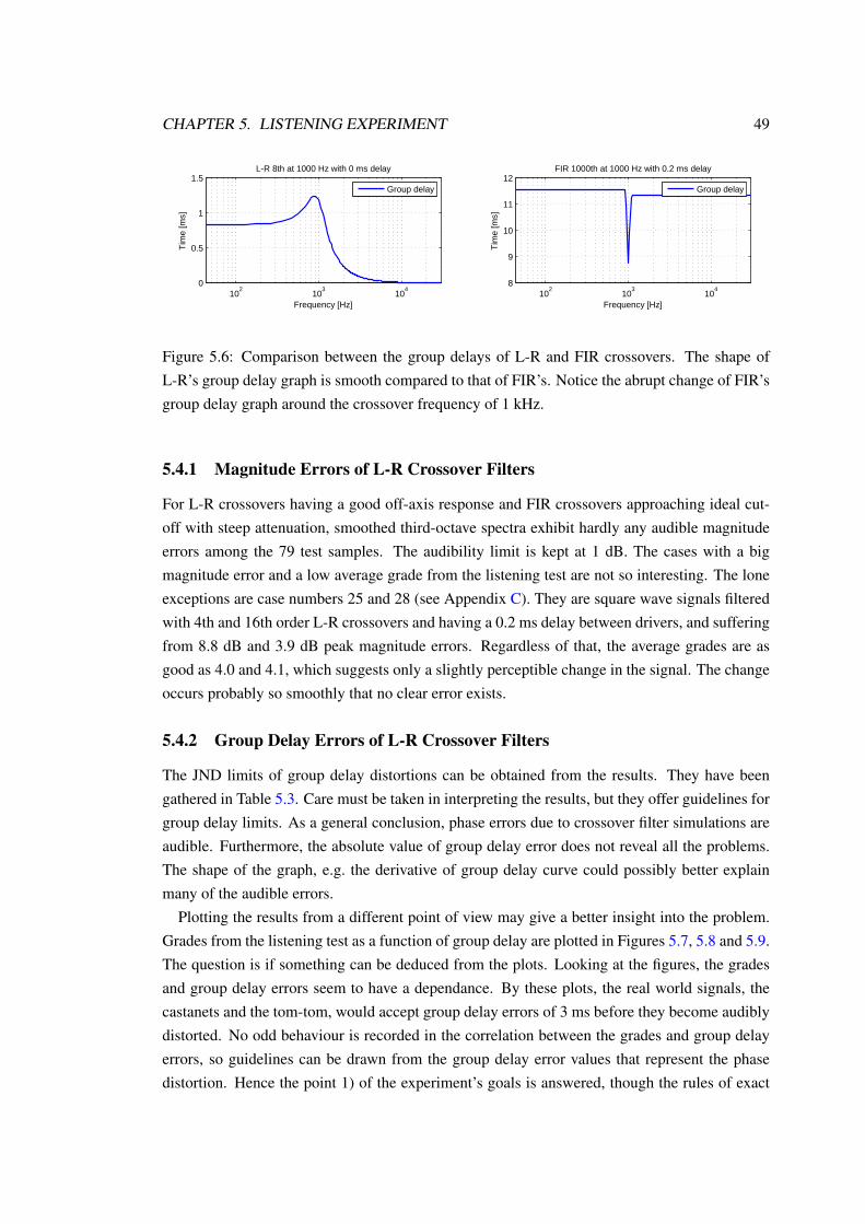
CHAPTER 5. LISTENING EXPERIMENT 49
102
103
104
0
0.5
1
1.5L-R 8th at 1000 Hz with 0 ms delay
Frequency [Hz]
Tim
e [m
s]
Group delay
102
103
104
8
9
10
11
12FIR 1000th at 1000 Hz with 0.2 ms delay
Frequency [Hz]
Tim
e [m
s]
Group delay
Figure 5.6: Comparison between the group delays of L-R and FIR crossovers. The shape ofL-R’s group delay graph is smooth compared to that of FIR’s. Notice the abrupt change of FIR’sgroup delay graph around the crossover frequency of 1 kHz.
5.4.1 Magnitude Errors of L-R Crossover Filters
For L-R crossovers having a good off-axis response and FIR crossovers approaching ideal cut-off with steep attenuation, smoothed third-octave spectra exhibit hardly any audible magnitudeerrors among the 79 test samples. The audibility limit is kept at 1 dB. The cases with a bigmagnitude error and a low average grade from the listening test are not so interesting. The loneexceptions are case numbers 25 and 28 (see Appendix C). They are square wave signals filteredwith 4th and 16th order L-R crossovers and having a 0.2 ms delay between drivers, and sufferingfrom 8.8 dB and 3.9 dB peak magnitude errors. Regardless of that, the average grades are asgood as 4.0 and 4.1, which suggests only a slightly perceptible change in the signal. The changeoccurs probably so smoothly that no clear error exists.
5.4.2 Group Delay Errors of L-R Crossover Filters
The JND limits of group delay distortions can be obtained from the results. They have beengathered in Table 5.3. Care must be taken in interpreting the results, but they offer guidelines forgroup delay limits. As a general conclusion, phase errors due to crossover filter simulations areaudible. Furthermore, the absolute value of group delay error does not reveal all the problems.The shape of the graph, e.g. the derivative of group delay curve could possibly better explainmany of the audible errors.
Plotting the results from a different point of view may give a better insight into the problem.Grades from the listening test as a function of group delay are plotted in Figures 5.7, 5.8 and 5.9.The question is if something can be deduced from the plots. Looking at the figures, the gradesand group delay errors seem to have a dependance. By these plots, the real world signals, thecastanets and the tom-tom, would accept group delay errors of 3 ms before they become audiblydistorted. No odd behaviour is recorded in the correlation between the grades and group delayerrors, so guidelines can be drawn from the group delay error values that represent the phasedistortion. Hence the point 1) of the experiment’s goals is answered, though the rules of exact
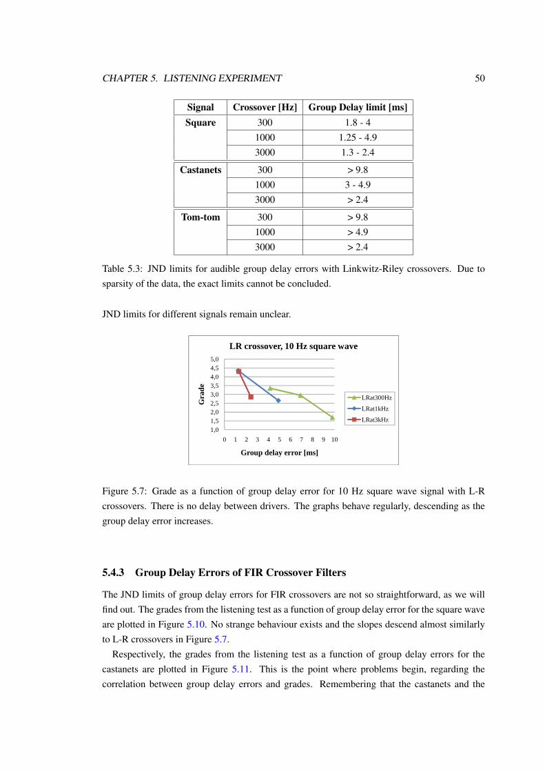
CHAPTER 5. LISTENING EXPERIMENT 50
Signal Crossover [Hz] Group Delay limit [ms]Square 300 1.8 - 4
1000 1.25 - 4.93000 1.3 - 2.4
Castanets 300 > 9.81000 3 - 4.93000 > 2.4
Tom-tom 300 > 9.81000 > 4.93000 > 2.4
Table 5.3: JND limits for audible group delay errors with Linkwitz-Riley crossovers. Due tosparsity of the data, the exact limits cannot be concluded.
JND limits for different signals remain unclear.
3,54,04,55,0
Gra
de
LR crossover, 10 Hz square wave
1,01,52,02,53,0
0 1 2 3 4 5 6 7 8 9 10
Gra
de
Group delay error [ms]
LRat300Hz
LRat1kHz
LRat3kHz
Figure 5.7: Grade as a function of group delay error for 10 Hz square wave signal with L-Rcrossovers. There is no delay between drivers. The graphs behave regularly, descending as thegroup delay error increases.
5.4.3 Group Delay Errors of FIR Crossover Filters
The JND limits of group delay errors for FIR crossovers are not so straightforward, as we willfind out. The grades from the listening test as a function of group delay error for the square waveare plotted in Figure 5.10. No strange behaviour exists and the slopes descend almost similarlyto L-R crossovers in Figure 5.7.
Respectively, the grades from the listening test as a function of group delay errors for thecastanets are plotted in Figure 5.11. This is the point where problems begin, regarding thecorrelation between group delay errors and grades. Remembering that the castanets and the
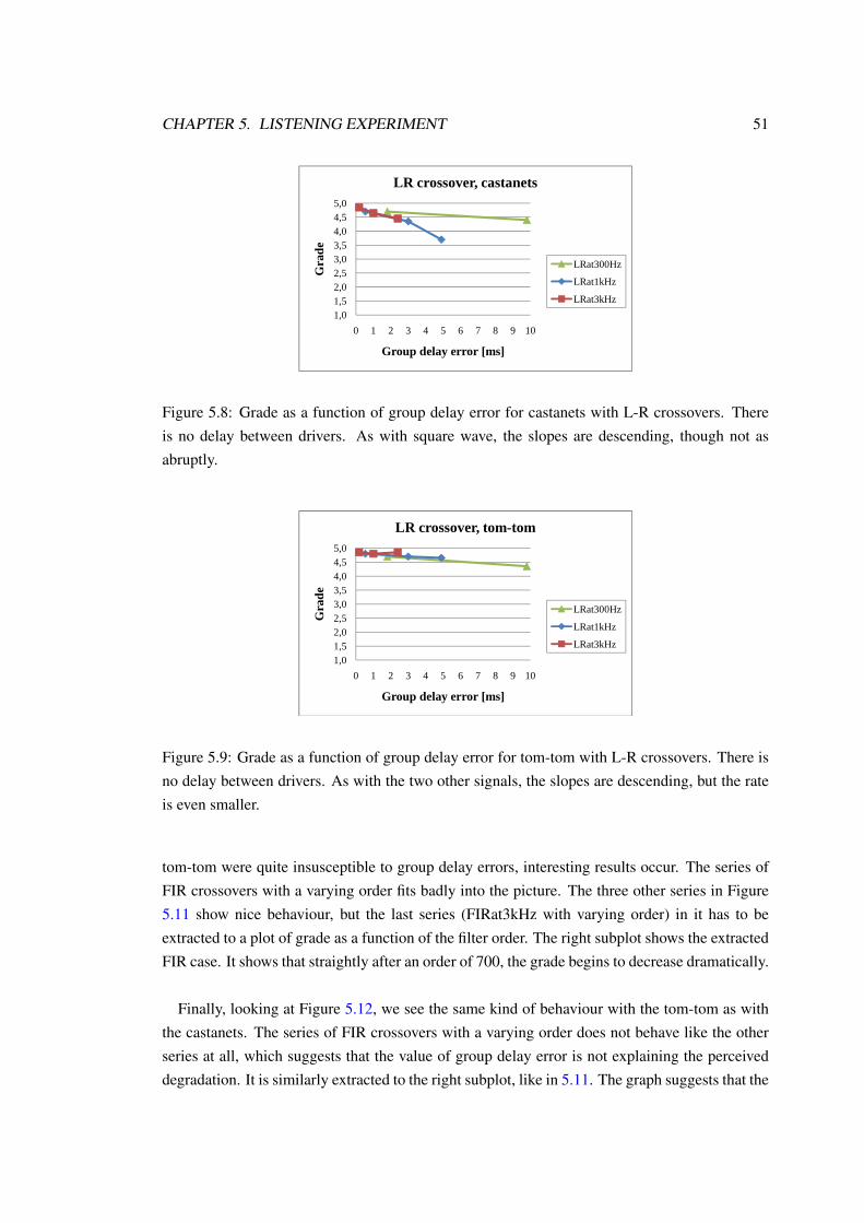
CHAPTER 5. LISTENING EXPERIMENT 51
3,54,04,55,0
Gra
de
LR crossover, castanets
1,01,52,02,53,0
0 1 2 3 4 5 6 7 8 9 10G
rade
Group delay error [ms]
LRat300Hz
LRat1kHz
LRat3kHz
Figure 5.8: Grade as a function of group delay error for castanets with L-R crossovers. Thereis no delay between drivers. As with square wave, the slopes are descending, though not asabruptly.
3,54,04,55,0
Gra
de
LR crossover, tom-tom
1,01,52,02,53,0
0 1 2 3 4 5 6 7 8 9 10
Gra
de
Group delay error [ms]
LRat300Hz
LRat1kHz
LRat3kHz
Figure 5.9: Grade as a function of group delay error for tom-tom with L-R crossovers. There isno delay between drivers. As with the two other signals, the slopes are descending, but the rateis even smaller.
tom-tom were quite insusceptible to group delay errors, interesting results occur. The series ofFIR crossovers with a varying order fits badly into the picture. The three other series in Figure5.11 show nice behaviour, but the last series (FIRat3kHz with varying order) in it has to beextracted to a plot of grade as a function of the filter order. The right subplot shows the extractedFIR case. It shows that straightly after an order of 700, the grade begins to decrease dramatically.
Finally, looking at Figure 5.12, we see the same kind of behaviour with the tom-tom as withthe castanets. The series of FIR crossovers with a varying order does not behave like the otherseries at all, which suggests that the value of group delay error is not explaining the perceiveddegradation. It is similarly extracted to the right subplot, like in 5.11. The graph suggests that the
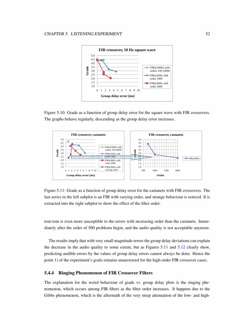
CHAPTER 5. LISTENING EXPERIMENT 52
3,54,04,55,0
Gra
de
FIR crossover, 10 Hz square wave
FIRat100Hz with
1,01,52,02,53,0
0 1 2 3 4 5 6 7 8 9 10G
rade
Group delay error [ms]
FIRat100Hz with orders 100,10000
FIRat1kHz with order 1000
FIRat3kHz with order 2000
Figure 5.10: Grade as a function of group delay error for the square wave with FIR crossovers.The graphs behave regularly, descending as the group delay error increases.
1,0
1,5
2,0
2,5
3,0
3,5
4,0
4,5
5,0
0 1 2 3 4 5 6 7 8 9 10
Gra
de
Group delay error [ms]
FIR crossover, castanets
FIRat100Hz with orders 100,10000
FIRat1kHz with order 2000
FIRat3kHz with order 2000
FIRat3kHz with varying order
1,0
1,5
2,0
2,5
3,0
3,5
4,0
4,5
5,0
500 1000 1500 2000
Gra
de
Order
FIR crossover, castanets
FIRat3kHz
Figure 5.11: Grade as a function of group delay error for the castanets with FIR crossovers. Thelast series in the left subplot is an FIR with varying order, and strange behaviour is noticed. It isextracted into the right subplot to show the effect of the filter order.
tom-tom is even more susceptible to the errors with increasing order than the castanets. Imme-diately after the order of 500 problems begin, and the audio quality is not acceptable anymore.
The results imply that with very small magnitude errors the group delay deviations can explainthe decrease in the audio quality to some extent, but as Figures 5.11 and 5.12 clearly show,predicting audible errors by the values of group delay errors cannot always be done. Hence thepoint 1) of the experiment’s goals remains unanswered for the high-order FIR crossover cases.
5.4.4 Ringing Phenomenon of FIR Crossover Filters
The explanation for the weird behaviour of grade vs. group delay plots is the ringing phe-nomenon, which occurs among FIR filters as the filter order increases. It happens due to theGibbs phenomenon, which is the aftermath of the very steep attenuation of the low- and high-

CHAPTER 5. LISTENING EXPERIMENT 53
1,0
1,5
2,0
2,5
3,0
3,5
4,0
4,5
5,0
0 1 2 3 4 5 6 7 8 9 10
Gra
de
Group delay error [ms]
FIR crossover, tom-tom
FIRat100Hz with orders 100,10000
FIRat1kHz with order 2000
FIRat3kHz with order 2000
FIRat3kHz with varying order
1,0
1,5
2,0
2,5
3,0
3,5
4,0
4,5
5,0
500 1000 1500 2000
Gra
de
Filter order
FIR crossover, tom-tom
FIRat3kHz
Figure 5.12: Grade as a function of group delay error for the tom-tom with FIR crossovers. Thelast series in the left subplot is an FIR with varying order, and strange behaviour is again noticed.It is extracted into the right subplot to show the effect of the filter order.
pass filters [10]. On-axis it is no problem, because the low- and highpass impulse responsessum up nicely, and the crossover filter impulse response is just a delayed impulse. Off-axis thesumming does not succeed and residual ringing will be left.
A comparison is made between two FIR samples with the castanets. Table 5.4 gathers theparameters. By the group delay error values, expecting a better grade for a 2000th order FIRcrossover would be realistic. However, the average grade of the 700th order FIR is 4.4, whilethe 2000th order FIR crossover has only received an average grade of 2.3. This seems counter-intuitive according to the values of magnitude and group delay errors. The only factor whichexplains the difference is the much higher order of the crossover filter, apparently offering im-pressive properties for a crossover filter, but eventually substantially degradating the signal.
Type Order Crossover[Hz]
Delay[ms]
Signal GrpDel Err[ms]
MagnErr [dB]
AvgGrade
FIR 700 3000 0.5 cast 2.25 0.6 4.4
FIR 2000 3000 0.5 cast 0.93 0.2 2.3
Table 5.4: Comparison of samples to demonstrate the ringing phenomenon. The delay betweendrivers is 0.5 ms. Magnitude error is decreasing from 0.6 to 0.2 dB. Judging from the groupdelay and magnitude error values, the 2000th order FIR should receive much better grade, butthe opposite is observed.
Regarding ringing in the time domain, zoomed plots of the impulse responses of 700th and2000th order FIR crossover filters simulated at an off-axis position are presented in Figure 5.13.As the theory [10] dictates, the height of the ripple is unchanged when the filter order is in-creased, but the width and the amount of ripples do change. This is clearly seen in Figure 5.13.The ringing lasts longer in the time domain in both sides of the main response.
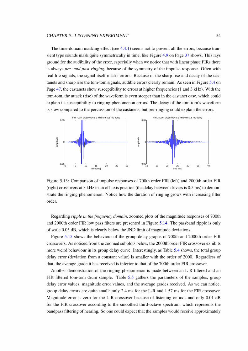
CHAPTER 5. LISTENING EXPERIMENT 54
The time-domain masking effect (see 4.4.1) seems not to prevent all the errors, because tran-sient type sounds mask quite symmetrically in time, like Figure 4.9 on Page 37 shows. This laysground for the audibility of the error, especially when we notice that with linear phase FIRs thereis always pre- and post-ringing, because of the symmetry of the impulse response. Often withreal life signals, the signal itself masks errors. Because of the sharp rise and decay of the cas-tanets and sharp rise the tom-tom signals, audible errors clearly remain. As seen in Figure 5.4 onPage 47, the castanets show susceptibility to errors at higher frequencies (1 and 3 kHz). With thetom-tom, the attack (rise) of the waveform is even steeper than in the castanet case, which couldexplain its susceptibility to ringing phenomenon errors. The decay of the tom-tom’s waveformis slow compared to the percussion of the castanets, but pre-ringing could explain the errors.
0 5 10 15 20 25 30-0.05
0
0.05
time [ms]
ampl
itude
FIR 700th crossover at 3 kHz with 0,5 ms delay
10 15 20 25 30 35 40-0.05
0
0.05
time [ms]
ampl
itude
FIR 2000th crossover at 3 kHz with 0,5 ms delay
Figure 5.13: Comparison of impulse responses of 700th order FIR (left) and 2000th order FIR(right) crossovers at 3 kHz in an off-axis position (the delay between drivers is 0.5 ms) to demon-strate the ringing phenomenon. Notice how the duration of ringing grows with increasing filterorder.
Regarding ripple in the frequency domain, zoomed plots of the magnitude responses of 700thand 2000th order FIR low pass filters are presented in Figure 5.14. The passband ripple is onlyof scale 0.05 dB, which is clearly below the JND limit of magnitude deviations.
Figure 5.15 shows the behaviour of the group delay graphs of 700th and 2000th order FIRcrossovers. As noticed from the zoomed subplots below, the 2000th order FIR crossover exhibitsmore weird behaviour in its group delay curve. Interestingly, as Table 5.4 shows, the total groupdelay error (deviation from a constant value) is smaller with the order of 2000. Regardless ofthat, the average grade it has received is inferior to that of the 700th order FIR crossover.
Another demonstration of the ringing phenomenon is made between an L-R filtered and anFIR filtered tom-tom drum sample. Table 5.5 gathers the parameters of the samples, groupdelay error values, magnitude error values, and the average grades received. As we can notice,group delay errors are quite small: only 2.4 ms for the L-R and 1.57 ms for the FIR crossover.Magnitude error is zero for the L-R crossover because of listening on-axis and only 0.01 dBfor the FIR crossover according to the smoothed third-octave spectrum, which represents thebandpass filtering of hearing. So one could expect that the samples would receive approximately
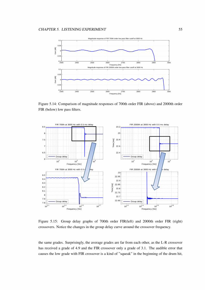
CHAPTER 5. LISTENING EXPERIMENT 55
2300 2400 2500 2600 2700 2800 2900 3000-0.1
-0.05
0
0.05
0.1Magnitude response of FIR 700th order low pass filter cutoff at 3000 Hz
Gai
n [d
B]
Frequency [Hz]
2300 2400 2500 2600 2700 2800 2900 3000-0.1
-0.05
0
0.05
0.1Magnitude response of FIR 2000th order low pass filter cutoff at 3000 Hz
Gai
n [d
B]
Frequency [Hz]
Figure 5.14: Comparison of magnitude responses of 700th order FIR (above) and 2000th orderFIR (below) low pass filters.
102
103
104
6
6.5
7
7.5
8
8.5FIR 700th at 3000 Hz with 0.5 ms delay
Frequency [Hz]
Tim
e [m
s]
Group delay
102
103
104
22.4
22.6
22.8
23
23.2FIR 2000th at 3000 Hz with 0.5 ms delay
Frequency [Hz]
Tim
e [m
s]
Group delay
8.5
FIR 700th at 3000 Hz with 0.5 ms delay 23
FIR 2000th at 3000 Hz with 0.5 ms delay
103.1
103.3
103.5
103.7
7.8
7.9
8
8.1
8.2
8.3
8.4
8.5
Frequency [Hz]
Tim
e [m
s]
Group delay
103.2
103.4
103.6
103.8
22.65
22.7
22.75
22.8
22.85
22.9
22.95
Frequency [Hz]
Tim
e [m
s]
Group delay
Figure 5.15: Group delay graphs of 700th order FIR(left) and 2000th order FIR (right)crossovers. Notice the changes in the group delay curve around the crossover frequency.
the same grades. Surprisingly, the average grades are far from each other, as the L-R crossoverhas received a grade of 4.9 and the FIR crossover only a grade of 3.1. The audible error thatcauses the low grade with FIR crossover is a kind of ”squeak” in the beginning of the drum hit,

CHAPTER 5. LISTENING EXPERIMENT 56
which is caused by pre-ringing phenomenon in the impulse response.
Type Order Crossover[Hz]
Delay[ms]
Signal GrpDel Err[ms]
MagnErr [dB]
AvgGrade
L-R 32 3000 0 tom-tom 2.4 0 4.9
FIR 2000 3000 0.03 tom-tom 1.57 0.01 3.1
Table 5.5: Comparison of samples to demonstrate the ringing phenomenon. The delay imple-mented to the FIR crossover is very small. Group delay errors are below the audibility limitsreceived. Magnitude error of FIR is increasingly small, only 0.01 dB, which is well below thegeneral perception level of 1 dB. Regardless, the average grades differ remarkably.
To study the problem more deeply, the impulse responses are first examined. They are plottedin Figure 5.16. There exists certain ringing in the L-R’s impulse response, but it is practicallydecayed off after 5-6 ms. The duration of FIR crossover’s ringing in the impulse response ismuch longer. Worth noting is also the asymmetry of the L-R’s impulse response. As the FIRcrossover is realised with linear phase, the impulse response has to be symmetric [10]. Thismakes the pre-ringing phenomenon easily audible, as the signal itself masks the errors wellforward with fast-rising, but slow-decaying sounds, such as the tom-tom. The same does nothappen backward.
-1 0 1 2 3 4 5 6 7 8-0.05
0
0.05
time [ms]
ampl
itude
L-R 32th crossover at 3 kHz
18 20 22 24 26 28 30-0.05
0
0.05
time [ms]
ampl
itude
FIR 2000th crossover at 3 kHz with 0,03 ms delay
Figure 5.16: Comparison of impulse responses of 32th order L-R (left) and 2000th order FIR(right) crossovers to demonstrate the ringing phenomenon. Notice the asymmetry in ringing ofL-R’s vs. the symmetry of FIR’s. The impulse responses are closely zoomed to illustrate thephenomenon better.
Zoomed plots of the magnitude responses of a 16th order Butterworth and a 2000th order FIRlowpass filters are shown in Figure 5.17. A 16th order Butterworth filter was used, because a32th order L-R is formed of two such Butterworth filters (for low- and highpass each) and Matlabhad numerical precision difficulties in computing a filter of 32th order.
Figure 5.18 shows the behaviour of group delay of these crossover filters. The L-R crossover’s

CHAPTER 5. LISTENING EXPERIMENT 57
500 1000 1500 2000 2500 3000 3500 4000-0.05
0
0.05Magnitude response of FIR 2000th order low pass filter cutoff at 3000 Hz
Gai
n [d
B]
Frequency [Hz]
500 1000 1500 2000 2500 3000 3500 4000-0.05
0
0.05Magnitude response of Butterworth 16th order low pass filter cutoff at 3000 Hz
Gai
n [d
B]
Frequency [Hz]
Figure 5.17: Comparison of magnitude responses of 16th order Butterworth (below) and 2000thorder FIR (above) lowpass filters.
group delay graph is on the left, and though it is not smooth, it does not have abnormalities init. The FIR crossover’s group delay graph is on the top right, and it has a very sudden changearound the crossover frequency. Furthermore, when the graph is zoomed around the crossoverfrequency, certain ripple can be seen in the graph.
The essential question is: which one is audible, the minimal ripple in the magnitude response,or the strange behaviour of the group delay response? Both degradations are below the generallyknown and obtained audibility limits of group delay (see the results of L-R in Table 5.3 on Page50) and of magnitude (see Figure 4.7 on Page 36), which makes it tricky. As hearing performsanalysis in both time- and frequency domains, the explanation for errors with high-order FIRcrossovers should be searched for with the time-domain analysis. This will be done in Chapter6.
However, the point 2) of the experiment’s goals on Page 41 can be answered after these twoinspections: High order FIR crossovers seem to be highly susceptible to off-axis errors. Thedelay of 0.03 ms corresponds only a flight time difference of 1 cm between the loudspeaker’sdrivers. This equals an off-axis position of only 2-3 degrees when the loudspeaker drivers areseparated by 0.25 m.
5.4.5 Effect of Training
An interesting point was the effect of training on the capability of perceiving group delay (phase)errors. The ability should become better, as e.g. Blauert and Laws state in their study [15]. In thelistening test, the grades between the trained listener (the author) and untrained (all the others)did not, however, differ from each other remarkably. Only a couple of differences above 1.0 wererecorded and the average standard deviation between the author’s grades and the participants’grades was 0.4 over the 79 samples. Notice that only one person was trained in this case, which

CHAPTER 5. LISTENING EXPERIMENT 58
102
103
104
0
0.5
1
1.5
2
2.5L-R 32th at 3000 Hz with 0 ms delay
Tim
e [m
s]
Group delay
102
103
104
21
21.5
22
22.5
23FIR 2000th at 3000 Hz with 0.03 ms delay
Tim
e [m
s]
Group delay
102
103
104
Frequency [Hz]10
210
310
4
Frequency [Hz]
103.3
103.4
103.5
103.6
103.7
22.45
22.5
22.55
22.6
22.65
22.7
22.75
FIR 2000th at 3000 Hz with 0.03 ms delay
Frequency [Hz]
Tim
e [m
s]
Group delay
Figure 5.18: Group delay graphs of L-R (left) and FIR (right) crossovers. Notice the abruptchanges of FIR crossover’s group delay around the crossover frequency in the zoomed subplot(bottom).
is not enough to make any conclusions.The training period for the test being minimal and affecting the difficulty to place the samples
on the grade scale, it can be concluded that in this case the effect of training was not helpingto perceive phase errors. A partial reason is that the exact limits were not found because of thesparsity of the data samples. A different type of test, such as adjustment by decreasing stepsto find the limits, could have recorded enhancement in the perception as the test subjects wouldhave gained experience.
5.5 Results and Analysis of Loudspeaker Listening Experiment
A real loudspeaker was also used for testing linear phase FIR crossover filters. Comparing theresults with headphone simulation was of interest. Five untrained persons participated in theexperiment. After seeing the results from headphone simulation, the test was decided to servefor finding the FIR filter orders that do not produce audible errors. The test signals used in theloudspeaker experiment were 10 Hz square wave and the castanets.
The listening positions in the listening room are depicted in Figure 5.19. The loudspeakerwas placed as the left channel in stereo listening (for position 1). The experiment consisted
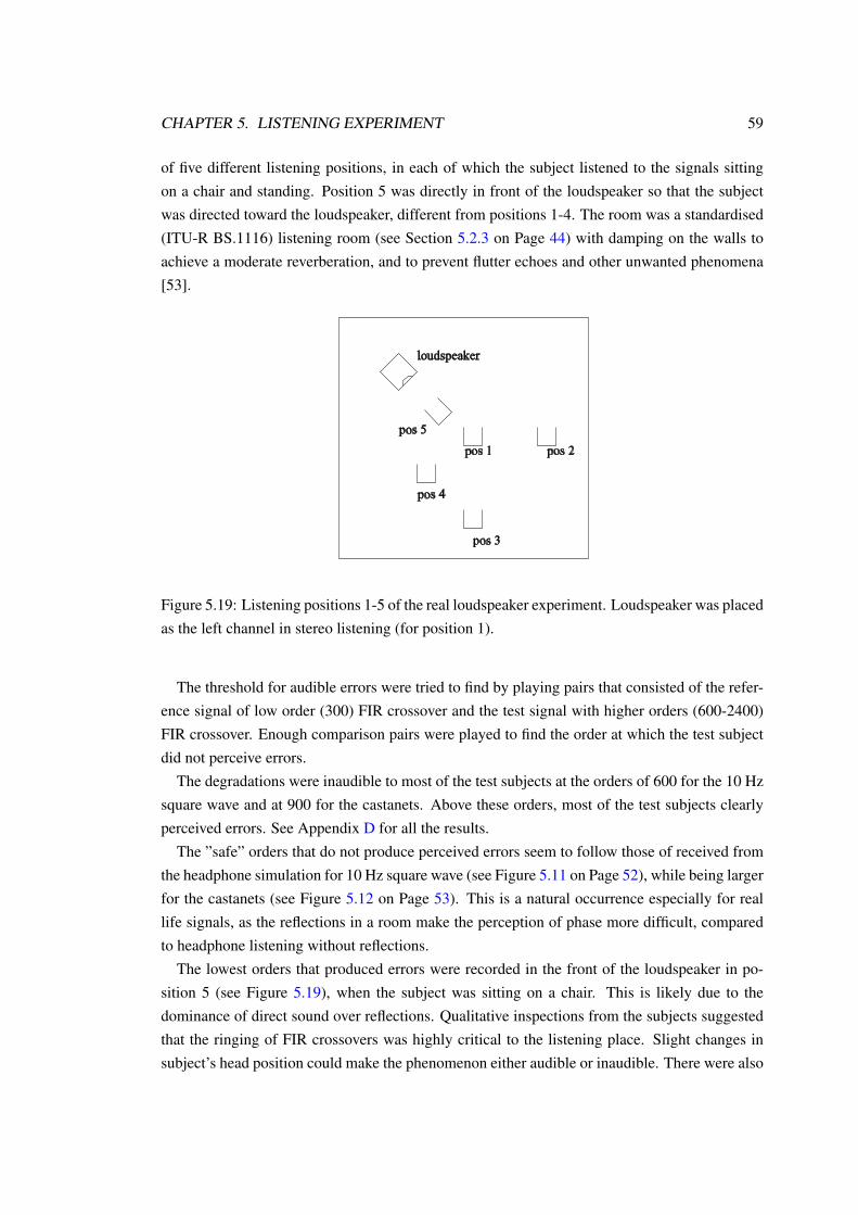
CHAPTER 5. LISTENING EXPERIMENT 59
of five different listening positions, in each of which the subject listened to the signals sittingon a chair and standing. Position 5 was directly in front of the loudspeaker so that the subjectwas directed toward the loudspeaker, different from positions 1-4. The room was a standardised(ITU-R BS.1116) listening room (see Section 5.2.3 on Page 44) with damping on the walls toachieve a moderate reverberation, and to prevent flutter echoes and other unwanted phenomena[53].
Figure 5.19: Listening positions 1-5 of the real loudspeaker experiment. Loudspeaker was placedas the left channel in stereo listening (for position 1).
The threshold for audible errors were tried to find by playing pairs that consisted of the refer-ence signal of low order (300) FIR crossover and the test signal with higher orders (600-2400)FIR crossover. Enough comparison pairs were played to find the order at which the test subjectdid not perceive errors.
The degradations were inaudible to most of the test subjects at the orders of 600 for the 10 Hzsquare wave and at 900 for the castanets. Above these orders, most of the test subjects clearlyperceived errors. See Appendix D for all the results.
The ”safe” orders that do not produce perceived errors seem to follow those of received fromthe headphone simulation for 10 Hz square wave (see Figure 5.11 on Page 52), while being largerfor the castanets (see Figure 5.12 on Page 53). This is a natural occurrence especially for reallife signals, as the reflections in a room make the perception of phase more difficult, comparedto headphone listening without reflections.
The lowest orders that produced errors were recorded in the front of the loudspeaker in po-sition 5 (see Figure 5.19), when the subject was sitting on a chair. This is likely due to thedominance of direct sound over reflections. Qualitative inspections from the subjects suggestedthat the ringing of FIR crossovers was highly critical to the listening place. Slight changes insubject’s head position could make the phenomenon either audible or inaudible. There were also
CHAPTER 5. LISTENING EXPERIMENT 60
differences between test subjects.Remarkable is that the errors were clearly audible with a real signal and a real loudspeaker
in a listening room. This suggests carefulness in designing and using digital crossover filters,especially linear phase FIR crossovers with higher orders.
5.6 Conclusions from the Listening Experiments
1. For Linkwitz-Riley crossovers, JND limits for group delay deviations vary between sig-nals, with the 10 Hz square wave being the most susceptible, the castanets being less sus-ceptible and the tom-tom being the least susceptible to phase distortions. The guidelinesfor JND limits can be read from Table 5.3 on Page 50.
2. For FIR crossovers, JND limits for group delay errors cannot be obtained, as no systematiccorrelation between group delay error values and grades exists.
3. The shape of the group delay graph might be crucial for perceived errors. FIR crossovers’group delay curves show irregularities compared to L-R crossover’s group delay curves.
4. FIR crossovers seem to be highly susceptible to off-axis errors with higher filter orders.The flight time difference of only 0.02-0.03 ms between low- and highpass bands at 3 kHzwas found to produce audible ringing with high FIR orders of the scale 1000-2000. Roughsafety limits would be to keep the order of a linear-phase FIR filter at/under 600 accordingto both the headphone simulation and the real loudspeaker experiment.
5. Predicting the results can be to some extent made for L-R crossovers by the group delayerror values. Prediction with FIR crossovers seem to be much more complicated, as theringing caused by the Gibbs phenomenon causes different behaviour with higher filterorders.
6. The apparent characteristics of an ”ideal” crossover filter turn out not to be pursuited at anycost, because ”brick-wall” attenuation with a linear phase response demands a relativelyhigh-order FIR filter, which is exposed to the ringing phenomenon.
7. It seems obvious that the auditory effect of ringing happens in the time domain. Thisbehaviour will be analysed further with an auditory analysis of hearing in Chapter 6.

Chapter 6
Auditory Analysis
Due to the complexity of hearing, it would be unrealistic to assume that a complete mathematicalmodel could be formed of it. Nonetheless, modelling would be useful in hearing research, inaudio and communication technology, and in medical technology. Computers and digital signalprocessing have offered a realistic possibility to build models of hearing. An auditory modelis a general concept of the modeling of hearing. The models are divided into classes, such aspsychoacoustic models, filterbank models, physiological models of the cochlea, hair cell models,and binaural models. This chapter presents the fundamentals of different auditory models andshows how a simple filterbank analysis of hearing is implemented to interpret the results ofthe listening test conducted in Chapter 5. Further analysis was needed, because the simplecorrelates (group delay, smoothed third-octave spectrum) did not seem to explain the resultswith high-order FIR crossover filters. Optimally, the model would help to fulfill the point 3) ofthe experiment’s goals by predicting how humans perceive the audio quality differences.
6.1 Different Auditory Models
The first computational auditory models were introduced in the 1960s and 1970s [54, 55, 56]followed by more modern models in the 1980s by Lyon, Slaney and others [57, 58, 59, 60, 61].The diversity of the models derives from the complexity of hearing. The author of a model hasto choose the level of details and complexity in the model to opt for and this can lead to severaldifferent outcomes.
In the assessment of audio quality, the ultimate goal is to get rid of time-consuming listeningtests to predict the subjective quality by some objective measures. Two different approaches,intrusive and non-intrusive models, are used [62]. Intrusive models use a reference signal formeasuring the audio quality, while non-intrusive models do not use a reference signal. Theprinciple of Auditory Spectrum Distance (ASD) was introduced by Karjalainen in 1985 [63],and it forms the basis for International Telecommunication Union’s standardized models ITU-TP.861 and P.862 and ITU-R BS.1387 [64, 65, 66]. The last one is better known as PEAQ, which
61
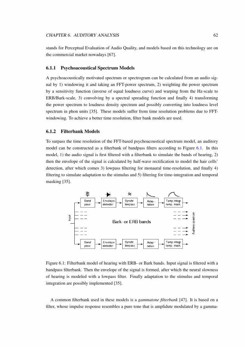
CHAPTER 6. AUDITORY ANALYSIS 62
stands for Perceptual Evaluation of Audio Quality, and models based on this technology are onthe commercial market nowadays [67].
6.1.1 Psychoacoustical Spectrum Models
A psychoacoustically motivated spectrum or spectrogram can be calculated from an audio sig-nal by 1) windowing it and taking an FFT-power spectrum, 2) weighting the power spectrumby a sensitivity function (inverse of equal loudness curve) and warping from the Hz-scale toERB/Bark-scale, 3) convolving by a spectral spreading function and finally 4) transformingthe power spectrum to loudness density spectrum and possibly converting into loudness levelspectrum in phon units [35]. These models suffer from time resolution problems due to FFT-windowing. To achieve a better time resolution, filter bank models are used.
6.1.2 Filterbank Models
To surpass the time resolution of the FFT-based psychoacoustical spectrum model, an auditorymodel can be constructed as a filterbank of bandpass filters according to Figure 6.1. In thismodel, 1) the audio signal is first filtered with a filterbank to simulate the bands of hearing, 2)then the envelope of the signal is calculated by half-wave rectification to model the hair cells’detection, after which comes 3) lowpass filtering for monaural time-resolution, and finally 4)filtering to simulate adaptation to the stimulus and 5) filtering for time-integration and temporalmasking [35].
Figure 6.1: Filterbank model of hearing with ERB- or Bark bands. Input signal is filtered with abandpass filterbank. Then the envelope of the signal is formed, after which the neural slownessof hearing is modeled with a lowpass filter. Finally adaptation to the stimulus and temporalintegration are possibly implemented [35].
A common filterbank used in these models is a gammatone filterbank [47]. It is based on afilter, whose impulse response resembles a pure tone that is amplidute modulated by a gamma-
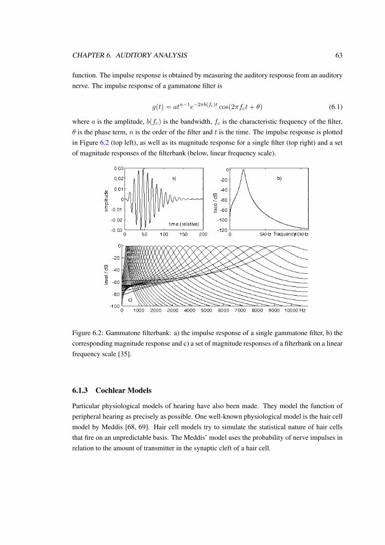
CHAPTER 6. AUDITORY ANALYSIS 63
function. The impulse response is obtained by measuring the auditory response from an auditorynerve. The impulse response of a gammatone filter is
g(t) = atn−1e−2πb(fc)t cos(2πfct+ θ) (6.1)
where a is the amplitude, b(fc) is the bandwidth, fc is the characteristic frequency of the filter,θ is the phase term, n is the order of the filter and t is the time. The impulse response is plottedin Figure 6.2 (top left), as well as its magnitude response for a single filter (top right) and a setof magnitude responses of the filterbank (below, linear frequency scale).
Figure 6.2: Gammatone filterbank: a) the impulse response of a single gammatone filter, b) thecorresponding magnitude response and c) a set of magnitude responses of a filterbank on a linearfrequency scale [35].
6.1.3 Cochlear Models
Particular physiological models of hearing have also been made. They model the function ofperipheral hearing as precisely as possible. One well-known physiological model is the hair cellmodel by Meddis [68, 69]. Hair cell models try to simulate the statistical nature of hair cellsthat fire on an unpredictable basis. The Meddis’ model uses the probability of nerve impulses inrelation to the amount of transmitter in the synaptic cleft of a hair cell.

CHAPTER 6. AUDITORY ANALYSIS 64
6.2 Auditory Analysis of the Listening Test
Simple auditory analysis was made, because the auditory correlates (group delay error andsmoothed third-octave spectrum error) discussed in Chapter 5 did not seem to help in predictingthe listening test results of high-order FIR crossover filters.
The ringing phenomenon was perceived clearly audible, even though both the group delayand magnitude error values were below the generally assumed audibility limits and the resultsreceived from the L-R crossovers’ listening tests. The first goal was to obtain qualitative under-standing of the temporal behaviour of crossover filtered signal in comparison with the original,unfiltered signal. Another goal would have been to predict the results of the listening test byobjective measure(s).
Qualitative analysis of the auditory analysis graphs turned out to be possible for FIR crossovers.For L-R crossovers, the analysis was not as informative. However, auditory analysis helped muchin interpreting the results and finding explanations for perceived phase errors.
6.2.1 Structure of Filterbank Model
A simple filterbank auditory analysis was used to analyse the results of the listening test. Becausethe degradations in the signals due to the crossover filters occurred in a narrow band, the externaland middle ear modeling were left out assuming that the auditory response is relatively flat inthe crossover region. The auditory analysis was implemented in Matlab and consisted of thefollowing steps:
1. Zero-phase (forward and backward) bandpass filtering using a bandpass Butterworth filterwith a bandwidth corresponding to Bark scale [35]:
∆fcb[Hz] = 25 + 75[1 + 1.4(fc[kHz])2]0.69 (6.2)
2. Full-wave rectification instead of half-wave rectification to smooth the response by takingthe absolute value of the signal.
3. Monaural time-resolution by 3rd order lowpass filtering at 300 Hz. No adaptation ortemporal integration (the last two blocks) of Figure 6.1 was used.
Filtering with Butterworth type filter was done with Matlab’s ”filtfilt”-function. A secondorder bandpass filter was applied three times both in forward and reverse directions, and zero-phase filter was thus obtained with smooth, symmetrical responses. Using a single Butterworthtype bandpass filter without reverse filtering (i.e. non-linear phase) was found to produce toomuch ripple in the auditory channel response, which made the interpretation more difficult, so itwas omitted. Time-alignment of original and crossover-simulated signals was also easier with azero-phase filter.
The magnitude responses of the used filterbank in three auditory channels are illustrated inFigure 6.3. The main auditory channel’s center frequency corresponds to the crossover frequency
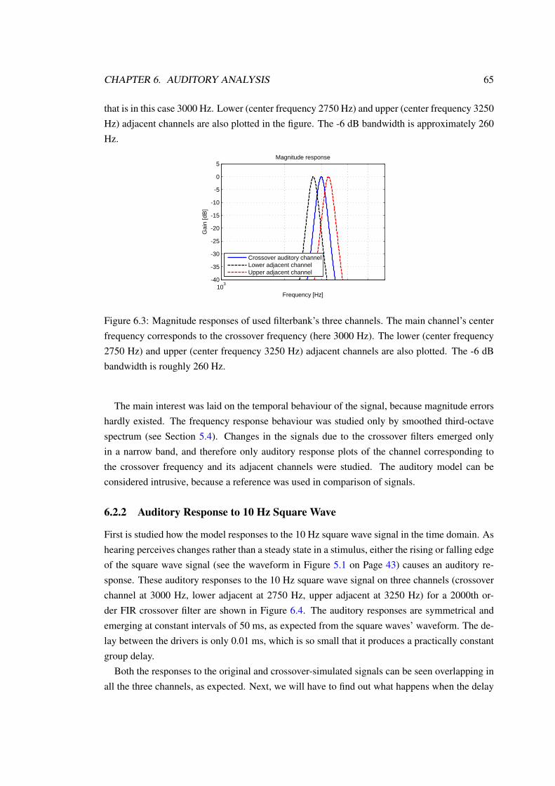
CHAPTER 6. AUDITORY ANALYSIS 65
that is in this case 3000 Hz. Lower (center frequency 2750 Hz) and upper (center frequency 3250Hz) adjacent channels are also plotted in the figure. The -6 dB bandwidth is approximately 260Hz.
103
-40
-35
-30
-25
-20
-15
-10
-5
0
5Magnitude response
Gai
n [d
B]
Frequency [Hz]
Crossover auditory channelLower adjacent channelUpper adjacent channel
Figure 6.3: Magnitude responses of used filterbank’s three channels. The main channel’s centerfrequency corresponds to the crossover frequency (here 3000 Hz). The lower (center frequency2750 Hz) and upper (center frequency 3250 Hz) adjacent channels are also plotted. The -6 dBbandwidth is roughly 260 Hz.
The main interest was laid on the temporal behaviour of the signal, because magnitude errorshardly existed. The frequency response behaviour was studied only by smoothed third-octavespectrum (see Section 5.4). Changes in the signals due to the crossover filters emerged onlyin a narrow band, and therefore only auditory response plots of the channel corresponding tothe crossover frequency and its adjacent channels were studied. The auditory model can beconsidered intrusive, because a reference was used in comparison of signals.
6.2.2 Auditory Response to 10 Hz Square Wave
First is studied how the model responses to the 10 Hz square wave signal in the time domain. Ashearing perceives changes rather than a steady state in a stimulus, either the rising or falling edgeof the square wave signal (see the waveform in Figure 5.1 on Page 43) causes an auditory re-sponse. These auditory responses to the 10 Hz square wave signal on three channels (crossoverchannel at 3000 Hz, lower adjacent at 2750 Hz, upper adjacent at 3250 Hz) for a 2000th or-der FIR crossover filter are shown in Figure 6.4. The auditory responses are symmetrical andemerging at constant intervals of 50 ms, as expected from the square waves’ waveform. The de-lay between the drivers is only 0.01 ms, which is so small that it produces a practically constantgroup delay.
Both the responses to the original and crossover-simulated signals can be seen overlapping inall the three channels, as expected. Next, we will have to find out what happens when the delay

CHAPTER 6. AUDITORY ANALYSIS 66
between low- and highpass outputs of the crossover filter is increased.
2 2.1 2.2 2.3 2.4 2.5 2.6 2.7 2.8 2.9 3
x 104
0
10
20
30
40
50
time [samples]
mag
nitu
de [d
B]
Auditory responses to original and simulated square wave 10 Hz signals with FIR 2000 order crossover at 3000 Hz with 0.01 ms delay
Original signal, fc at 3000 HzSimulated signal, fc at 3000 Hz
2 2.1 2.2 2.3 2.4 2.5 2.6 2.7 2.8 2.9 3
x 104
0
10
20
30
40
50
time [samples]
mag
nitu
de [d
B]
Original signal, fc at 2750 HzSimulated signal, fc at 2750 Hz
2 2.1 2.2 2.3 2.4 2.5 2.6 2.7 2.8 2.9 3
x 104
0
10
20
30
40
50
time [samples]
mag
nitu
de [d
B]
Original signal, fc at 3250 HzSimulated signal, fc at 3250 Hz
Figure 6.4: Auditory analysis responses to 10 Hz square wave signal with 2000th order FIRcrossover filter on three adjacent auditory channels: 3000 Hz (crossover channel, top subplot),2750 Hz (lower channel, middle subplot), and 3250 Hz (upper channel, bottom subplot). Thedelay between drivers is 0.01 ms. The responses are symmetrical, emerging at constant intervalsand are overlapping nicely, and no perceivable difference is expected. The average grade fromthe listening test was 4.5.
Figure 6.5 shows the spreading of the time domain response for the same FIR 2000th ordercrossover at 3 kHz when the delay between the loudspeaker drivers is increased from 0.01 to0.02 ms. Though behaving quite nicely on the lower and upper auditory channels, the crossover-simulated signal response is vastly spread on the auditory channel of 3000 Hz, which correspondsto the crossover frequency. In spite of the group delay error being 1.57 ms, very clearly audibleringing is heard when listened in the test. The case of FIR 2000th order crossover at 3 kHz with0.02 ms delay has received an average grade of 2.8, which implies a clear degradation in audioquality. The parameters and errors of these two cases with 0.01 ms and 0.02 ms delays betweendrivers have been gathered in Table 6.1.
A contrasting demonstration of the effect of the ringing phenomenon is shown in Figure 6.6.

CHAPTER 6. AUDITORY ANALYSIS 67
Type Order Crossover[Hz]
Delay[ms]
Signal GrpDel Err[ms]
MagnErr [dB]
AvgGrade
FIR 2000 3000 0.01 square 0 0.001 4.5
FIR 2000 3000 0.02 square 1.57 0.01 2.8
Table 6.1: Comparison of samples that are used to demonstrate the ringing phenomenon. Theincrease of delay is very small. Group delay error is on the audibility limit according to L-Rcrossover’s results. Magnitude error of FIR is also very small, only 0.01 dB, which is well belowthe JND threshold of 1 dB.
2 2.1 2.2 2.3 2.4 2.5 2.6 2.7 2.8 2.9 3
x 104
0
10
20
30
40
50
time [samples]
mag
nitu
de [d
B]
Auditory responses to original and simulated square wave 10 Hz signals with FIR 2000 order crossover at 3000 Hz with 0.02 ms delay
Original signal, fc at 3000 HzSimulated signal, fc at 3000 Hz
2 2.1 2.2 2.3 2.4 2.5 2.6 2.7 2.8 2.9 3
x 104
0
10
20
30
40
50
time [samples]
mag
nitu
de [d
B]
Original signal, fc at 2750 HzSimulated signal, fc at 2750 Hz
2 2.1 2.2 2.3 2.4 2.5 2.6 2.7 2.8 2.9 3
x 104
0
10
20
30
40
50
time [samples]
mag
nitu
de [d
B]
Original signal, fc at 3250 HzSimulated signal, fc at 3250 Hz
Figure 6.5: Auditory analysis responses to 10 Hz square wave signal with 2000th order FIRcrossover filter on three adjacent auditory channels: 3000 Hz (crossover channel, top subplot),2750 Hz (lower channel, middle subplot), and 3250 Hz (upper channel, bottom subplot). Thedelay between drivers is now 0.02 ms. The crossover-simulated signal response is clearly spreadin time on the auditory channel corresponding to the crossover frequency, which is heard asaudible ringing in the sample. The average grade was 2.8.

CHAPTER 6. AUDITORY ANALYSIS 68
It illustrates the auditory response to the 10 Hz square wave with a 32th order L-R crossover at3 kHz on the main axis (delay between drivers is zero). The parameters and response errors ofthe sample have been gathered in Table 6.2 together with an off-axis sample of the same L-Rcrossover.
Studying the on-axis case, it can be seen that despite of the group delay error of 2.4 ms, whichis clearly audible according to the average grade of 2.9 from the listening test, the L-R crossoverfilter’s time domain auditory response shows only slight difference between the original andcrossover simulated samples, as Figure 6.6 illustrates. However, when the crossover-simulatedsignal responses in all the three channels are zoomed in and plotted in Figure 6.7, the effectof changing group delay is seen. This is an example of different phase error than with FIRcrossover’s ringing that causes spreading in time.
Studying the off-axis case, the auditory response to the 10 Hz square wave signal with L-R32th order crossover off the main axis is shown in Figure 6.8. The delay between drivers is now0.2 ms. Now the auditory response to the square wave shows a clearer difference between theoriginal and crossover simulated signals. The response curve has a bump on the left side on thecrossover channel at 3 kHz, while the adjacent channels do not seem to have any abnormalities.It must be remembered that this sample has a magnitude error larger than 2 dB, which is abovethe JND limit.
Comparing Figure 6.6 on Page 69 with Figure 6.5 on Page 67, it can be concluded that theringing phenomenon of FIR crossovers causes different degradations than L-R crossovers’ phaseerrors. Spreading in time is characteristic for FIR crossovers, whereas different group delays be-tween channels cause the audible phase errors with L-R crossovers. The ringing phenomenonwith FIR crossovers is seen more clearly in auditory responses than slight differences in chan-nels’ group delays with L-R crossovers.
One interpretation for audible distortion can be the abrupt changes in the group delay, asdiscussed in Chapter 5. The FIR crossover possesses a different group delay curve than theL-R crossover (see Figure 5.6). The ”leap” between the low- and highpass bands at (or near)the crossover frequency of an FIR crossover might be crucial for producing the errors. Thefrequency derivative of the group delay curve might be used as a criterion.
The asymmetry of the L-R crossover’s impulse response compared to the symmetry of theFIR crossover’s impulse response can also have an influence on the errors perceived. Pre-ringingcauses the error to be formed in the beginning (or before) the actual signal and not being maskedby the signal itself, which then causes the auditory response degradation.
6.2.3 Auditory Response to Castanets
Another illustration of the ringing phenomenon is presented in Figures 6.9 and 6.10. Table 5.4on Page 53 gathers the parameters of the samples. Figure 6.9 shows the auditory responses tothe castanet signal with a 700th order FIR crossover, suffering from weird behaviour at the topof the graph, but still receiving an average grade of 4.4, which means no audible distortion.
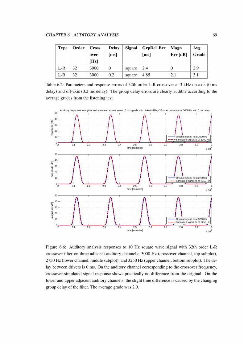
CHAPTER 6. AUDITORY ANALYSIS 69
Type Order Crossover[Hz]
Delay[ms]
Signal GrpDel Err[ms]
MagnErr [dB]
AvgGrade
L-R 32 3000 0 square 2.4 0 2.9
L-R 32 3000 0.2 square 4.85 2.1 3.1
Table 6.2: Parameters and response errors of 32th order L-R crossover at 3 kHz on-axis (0 msdelay) and off-axis (0.2 ms delay). The group delay errors are clearly audible according to theaverage grades from the listening test.
2 2.1 2.2 2.3 2.4 2.5 2.6 2.7 2.8 2.9 3
x 104
0
10
20
30
40
50
time [samples]
mag
nitu
de [d
B]
Auditory responses to original and simulated square wave 10 Hz signals with Linkwitz-Riley 32 order crossover at 3000 Hz with 0 ms delay
Original signal, fc at 3000 HzSimulated signal, fc at 3000 Hz
2 2.1 2.2 2.3 2.4 2.5 2.6 2.7 2.8 2.9 3
x 104
0
10
20
30
40
50
time [samples]
mag
nitu
de [d
B]
Original signal, fc at 2750 HzSimulated signal, fc at 2750 Hz
2 2.1 2.2 2.3 2.4 2.5 2.6 2.7 2.8 2.9 3
x 104
0
10
20
30
40
50
time [samples]
mag
nitu
de [d
B]
Original signal, fc at 3250 HzSimulated signal, fc at 3250 Hz
Figure 6.6: Auditory analysis responses to 10 Hz square wave signal with 32th order L-Rcrossover filter on three adjacent auditory channels: 3000 Hz (crossover channel, top subplot),2750 Hz (lower channel, middle subplot), and 3250 Hz (upper channel, bottom subplot). The de-lay between drivers is 0 ms. On the auditory channel corresponding to the crossover frequency,crossover-simulated signal response shows practically no difference from the original. On thelower and upper adjacent auditory channels, the slight time difference is caused by the changinggroup delay of the filter. The average grade was 2.9.

CHAPTER 6. AUDITORY ANALYSIS 70
315 320 325 330 335 340 3450
10
20
30
40
50
time [ms]
mag
nitu
de [d
B]
Simulated signal, fc at 3000 HzSimulated signal, fc at 2750 HzSimulated signal, fc at 3250 Hz
Figure 6.7: Auditory analysis responses to 10 Hz square wave signal with 32th order L-Rcrossover filter on three auditory channels without the original signal: 3000 Hz (crossover chan-nel), 2750 Hz (lower channel), and 3250 Hz (upper channel). The delay between drivers is 0ms. Notice how the responses differ in time due to changing group delay of the L-R crossover,producing audible phase errors.
On the contrary, Figure 6.10 illustrates the auditory responses to the castanets with a 2000thorder FIR crossover, and clear spreading is noticed. This means audible ringing in the sample,just as with the 10 Hz square wave signal. The smoothed third-octave spectra present only 0.6and 0.2 dB magnitude errors and 2.25 and 0.93 ms group delay errors for 700th and 2000th orderFIR crossovers, respectively. So both the group delay error and the magnitude error decrease asthe order increases, but the average grade decreases from 4.4 for 700th order FIR crossover to2.3 for 2000th order FIR crossover.
Analysing and noticing audible errors of FIR crossover filters may thus demand both analysingthe group delay and magnitude error values as well as time domain analysis of the auditoryresponses.
6.2.4 Conclusions from Auditory Analysis
1. When phase errors are studied, L-R crossovers show completely different auditory re-sponse (differences in channels’ group delays, see Figure 6.6 on Page 69) than high-orderFIR crossovers (spreading in time, see Figure 6.5 on Page 67). Off the main axis, theauditory responses of L-R crossovers show clearer abnormalities (see Figure 6.8 on Page71).
2. The ringing phenomenon caused by the Gibbs phenomenon in high-order FIR crossoversseems to be visible in the auditory responses to 10 Hz square wave and castanet signals,which helps to predict the degradations (see Figure 6.10 on Page 73), when the group delayerror values do not imply any degradation. The tom-tom drum has so complex waveformthat auditory analysis could not be interpreted in practice.

CHAPTER 6. AUDITORY ANALYSIS 71
2 2.1 2.2 2.3 2.4 2.5 2.6 2.7 2.8 2.9 3
x 104
0
10
20
30
40
50
time [samples]
mag
nitu
de [d
B]
Auditory responses to original and simulated square wave 10 Hz signals with Linkwitz-Riley 32 order crossover at 3000 Hz with 0.2 ms delay
Original signal, fc at 3000 HzSimulated signal, fc at 3000 Hz
2 2.1 2.2 2.3 2.4 2.5 2.6 2.7 2.8 2.9 3
x 104
0
10
20
30
40
50
time [samples]
mag
nitu
de [d
B]
Original signal, fc at 2750 HzSimulated signal, fc at 2750 Hz
2 2.1 2.2 2.3 2.4 2.5 2.6 2.7 2.8 2.9 3
x 104
0
10
20
30
40
50
time [samples]
mag
nitu
de [d
B]
Original signal, fc at 3250 HzSimulated signal, fc at 3250 Hz
Figure 6.8: Auditory analysis responses to 10 Hz square wave signal with 32th order L-Rcrossover filter off-axis on three adjacent auditory channels: 3000 Hz (crossover channel, topsubplot), 2750 Hz (lower channel, middle subplot), and 3250 Hz (upper channel, bottom sub-plot). The delay between drivers is 0.2 ms. On the auditory channel corresponding to thecrossover frequency, crossover-simulated signal response shows a bump on the left side. Theaverage grade was 3.1.
3. Quantitative measures of audio quality are challenging to find because of parallel time andfrequency domain analysis of hearing. From points 1) and 2) it can be concluded thateither group delay error values, magnitude error values, or temporal auditory analysis byinspection reveals the degradation in a signal. The L-R crossovers seem to correlate betterwith the group delay error values, while high-order FIR crossovers may show qualitativelyclearer degradations in the auditory responses.

CHAPTER 6. AUDITORY ANALYSIS 72
1.4 1.6 1.8 2 2.2 2.4 2.6 2.8
x 104
0
10
20
30
40
50
time [samples]
mag
nitu
de [d
B]
Auditory responses to original and simulated castanets signals with FIR 700 order crossover at 3000 Hz with 0.5 ms delay
Original signal, fc at 3000 HzSimulated signal, fc at 3000 Hz
1.4 1.6 1.8 2 2.2 2.4 2.6 2.8
x 104
0
10
20
30
40
50
time [samples]
mag
nitu
de [d
B]
Original signal, fc at 2750 HzSimulated signal, fc at 2750 Hz
1.4 1.6 1.8 2 2.2 2.4 2.6 2.8
x 104
0
10
20
30
40
50
time [samples]
mag
nitu
de [d
B]
Original signal, fc at 3250 HzSimulated signal, fc at 3250 Hz
Figure 6.9: Auditory analysis responses to castanet signal with 700th order FIR crossover filteron three adjacent auditory channels: 3000 Hz (crossover channel, top subplot), 2750 Hz (lowerchannel, middle subplot), and 3250 Hz (upper channel, bottom subplot). The delay betweendrivers is 0.5 ms. The center channel has a center frequency corresponding to the crossoverfrequency. On that auditory channel, the crossover simulated signal response is flattened fromthe top, but not much spread. The average grade was 4.4.

CHAPTER 6. AUDITORY ANALYSIS 73
1.4 1.6 1.8 2 2.2 2.4 2.6 2.8
x 104
0
10
20
30
40
50
time [samples]
mag
nitu
de [d
B]
Auditory responses to original and simulated castanets signals with FIR 2000 order crossover at 3000 Hz with 0.5 ms delay
Original signal, fc at 3000 HzSimulated signal, fc at 3000 Hz
1.4 1.6 1.8 2 2.2 2.4 2.6 2.8
x 104
0
10
20
30
40
50
time [samples]
mag
nitu
de [d
B]
Original signal, fc at 2750 HzSimulated signal, fc at 2750 Hz
1.4 1.6 1.8 2 2.2 2.4 2.6 2.8
x 104
0
10
20
30
40
50
time [samples]
mag
nitu
de [d
B]
Original signal, fc at 3250 HzSimulated signal, fc at 3250 Hz
Figure 6.10: Auditory analysis responses to castanet signal with 2000th order FIR crossover filteron three adjacent auditory channels: 3000 Hz (crossover channel, top subplot), 2750 Hz (lowerchannel, middle subplot), and 3250 Hz (upper channel, bottom subplot). The delay betweendrivers is 0.5 ms. On the auditory channel corresponding to the crossover frequency, crossoversimulated signal response is flattened from the top, and also clearly spread in time. The averagegrade was 2.3.

Chapter 7
Conclusions and Future Work
This thesis presented a perceptual study of digital loudspeaker crossover filters, which are re-sponsible for dividing the audio spectrum of a signal to corresponding loudspeaker units. A dig-ital implementation of a well-known analog crossover filter, called Linkwitz-Riley (L-R), wassimulated in Matlab software together with a purely digital FIR crossover filter that is capable ofapproaching the ”ideal” characteristics of low- and highpass filters with brick-wall attenuationand linearity in phase response.
A listening test was planned and conducted with a laptop computer and headphones to ex-amine perceptually the crossover filters’ effect on the sound quality. A minor listening test wasconducted with a loudspeaker in a listening room to compare the differences between headphoneand loudspeaker reproduction.
Artificial and real sound signals were used to get both an analytical and a practical pointof view. Magnitude and phase errors in the signals were studied and just noticeable levels ofdegradations due to different reasons were tried to obtain. Correspondence to recent studies ofthe audibility of phase errors [22] was of considerable interest. The FIR crossover that apparentlyhas nearly ”ideal” characteristics with uniform magnitude response and linear phase response onthe main axis was of the biggest interest, because practically no perceptual studies were foundon the topic.
The results were analysed with simple auditory correlates, such as group delay deviation froma constant value (phase error) or smoothed third-octave spectrum, which represents the spectrumanalysis of hearing (magnitude error). Also a more specific filterbank analysis of hearing wasimplemented in Matlab and was used to interpret the results when audible ringing was perceived.
The results and analysis of the listening test show that phase errors can be heard differentlywith different signals. The approximate JND limits for group delay errors with the L-R crossoverfilter seem to follow the rule of thumb (1.6 ms, [22]), when listening to 10 Hz square wave signal.For real life signals, such as the castanets, the JND limits seem to be higher, from 3-5 ms at highfrequencies (1 and 3 kHz) to over 10 ms at low frequency (300 Hz).
The group delay error limits with FIR crossover filters cannot be deciphered straightly from
74

CHAPTER 7. CONCLUSIONS AND FUTURE WORK 75
the group delay error values, because the ringing phenomenon with high-order FIRs caused bythe Gibbs phenomenon degrades the signal so that group delay error does not correlate withperceived degradations. The effect is only and essentially present, when listening off the mainaxis, and it becomes increasingly disturbing as the filter order increases. Already a very smallmovement off the main listening axis seems to produce clearly audible errors with high-orderdigital FIR crossovers, as only a flight time difference of 0.02 ms with an artificial signal and0.03-0.05 ms with real life signals at the crossover frequency of 3 kHz were perceived distortingin the listening test. With low-order FIRs the ringing effect does not appear as much as withhigh-order FIRs.
Hence, pursuiting of the ”ideal” reproduction of a signal seems to be good on the paper, butperceptual tests, with headphone simulation and a real loudspeaker, show that hearing clearlyperceives ringing degradations in the audio quality with both analytical and real life signals.Rough safety limits according to both test methods would be to keep the order of a linear phaseFIR crossover filter under 600 at higher frequencies (1 and 3 kHz) to prevent from the ringingphenomenon producing audible errors. At low frequencies, such as 100 Hz and 300 Hz, theorder may be up to thousands, and still no audible errors will occur.
Predicting the results of a listening test by some objective measure would be comfortable as areplacement to the tests. Thus correlations between the audio quality degradations and auditorymeasures were tried to find. With the L-R crossover filter, correlations could be found, as thegroup delay errors seemed to correlate fairly well with the evaluated quality. With high-orderFIR crossover filters, correlations seemed to be unsolved, because the increasing filter ordercaused degradations that did not correlate with the group delay error values.
Therefore different type of analysis is needed for revealing the audible errors of FIR crossoverfilters. A simple auditory analysis, which tries to model the function of peripheral hearing, wasused in the thesis. It shows qualitatively the degradations caused by the ringing phenomenonwith high-order FIR crossover filters, which the group delay error values do not imply. Phaseerrors caused by the L-R crossover’s group delay were also shown in the auditory analysis,though the degraded auditory responses were totally different from FIR crossovers’ responses.The shapes of the response graphs and the behaviour of them being complex, no quantitativemeasures could be found in this study, which is considered preliminary just for understandingthe related phenomena.
The abrupt changes in the group delay of a filter might be crucial for the audible errors, asthere are fundamental differences between L-R crossovers’ and high-order FIR crossovers’ groupdelay curves. However, either the magnitude or group delay error values or the auditory analysisreveal the audible errors.
Future work could include the quantification of more exact limits of the audible group delayerrors with a broad set of signals. Also more exact limits of the FIR filter order that begin tocause degradations would be interesting to find out. More experiments should be laid on howchanges in the group delay are affecting the perceived distortion. In listening experiment, a

CHAPTER 7. CONCLUSIONS AND FUTURE WORK 76
different test method to adjust the degradation in asymptotic steps toward the JND limits couldbe used. In the present study, it was considered too massive to conduct. Audiometry tests shouldalso be a part of the preparations for the listening test. One of the drawbacks of the study was thelack of training prior to the listening test, especially when it is known to help in the perceptionof small phase errors [15].
Building an auditory model that would predict the perception of humans by error values orby auditory analysis responses would be useful. It would require careful tuning of the auditorymodel relative to the results of listening tests. First, a predictor for JND degradations withsynthetic signals, such as the square wave, should be found. A more general model would predictthe degradation Mean Opinion Scores (MOS) with arbitrary signals. Such models commonlyneed a ”cognitive model” in addition to the peripheral model of hearing. A more generalisedmodel would also be able to predict MOS gradings for other types of degradations, not only formagnitude and/or phase degradations. The present work may lay ground for such development.
Bibliography
[1] J. Borwick. The Loudspeaker and Headphone Handbook. Focal Press, Oxford, 2nd edition,1994. 601 pages.
[2] M. Colloms. High Performance Loudspeakers. Pentech Press, London, 4th edition, 1991.407 pages.
[3] J. Strutt (Baron Rayleigh). The Theory of Sound, volume 2. MacMillan and Co., London,2nd edition, 1896.
[4] H. Kuttruff. Room Acoustics. Spon Press, London, 4th edition, 2000. 349 pages.
[5] A. V. Oppenheim and A. S. Willsky with I. T. Young. Signals and Systems. Prentice-HallInternational, USA, 1983.
[6] S. Linkwitz. Active crossover networks for noncoincident drivers. Journal of the AudioEngineering Society, 24(1):2–8, Jan/Feb 1976.
[7] S. P. Lipshitz and J. Vanderkooy. A family of linear-phase crossover networks of high slopederived by time delay. Journal of the Audio Engineering Society, 31:2–20, Jan/Feb 1983.
[8] N. Thiele. Implementing asymmetrical crossovers. Journal of the Audio Engineering So-ciety, 55(10):819–832, October 2007.
[9] R. H. Small. Constant-voltage crossover network design. Journal of the Audio EngineeringSociety, 19(1):12–19, January 1971.
[10] S. K. Mitra. Digital Signal Processing: A Computer-Based Approach. McGraw-Hill,Singapore, 1998. 864 pages.
[11] S. Linkwitz. Passive crossover networks for noncoincident drivers. Journal of the AudioEngineering Society, 26(3):149–150, 1978.
[12] B. B. Bauer. Audibility of phaseshift. Wireless World, April 1974.
[13] S. Linkwitz. www.linkwitzlab.com. World Wide Web, October 2007.
77

BIBLIOGRAPHY 78
[14] S. P. Lipshitz, M. Pocock, and J. Vanderkooy. On the audibility of midrange phase dis-tortion in audio systems. In The 67th Convention of the Audio Engineering Society, NewYork, October 1980.
[15] J. Blauert and P. Laws. Group delay distortions in electroacoustical systems. Journal ofthe Audio Engineering Society, (63(5)), May 1978.
[16] H. Suzuki, S. Morita, and T. Shindo. On the perception of phase distortion. Journal of theAudio Engineering Society, 28(9):570–574, February 1980.
[17] E. B. Jensen and H. Moller. On the audibility of phase distortion in audio systems. In The47th Convention of the Audio Engineering Society, Copenhagen, March 1974.
[18] J. A. Deer and P. J. Bloom. Perception of phase distortion in all-pass filters. In The 77thConvention of the Audio Engineering Society, Hamburg, March 1985.
[19] L.R. Fincham. The subjective importance of uniform group delay at low frequencies. InThe 74th Convention of the Audio Engineering Society, New York, October 1983.
[20] G. J. Krauss. On the audibility of group distortion at low frequencies. In The 88th Conven-tion of the Audio Engineering Society, Montreaux, March 1990.
[21] H. D. Harwood. Audibility of phase effects in loudspeakers. Wireless World, pages 30–32,January 1976.
[22] H. Moller, P. Minnaar, S. K. Olesen, F. Christensen, and J. Plogsties. On the audibilityof all-pass phase in electroacoustical transfer functions. Journal of the Audio EngineeringSociety, 55(3):115–134, May 2007.
[23] D. A. Bohn. Investigating 4th order active bessel crossovers. In The 81st Convention of theAudio Engineering Society, Los Angeles, November 1986.
[24] B. C. J. Moore. An Introduction to the Psychology of Hearing. Elsevier Academic Press,London, 2004. 413 pages.
[25] R. Chalupa. A subtractive implementation of Linkwitz-Riley crossover design. In The 78thConvention of the Audio Engineering Society, Anaheim, California, May 1986.
[26] A. Rimell and M. O. Hawksford. Digital crossover design strategy for drive units withimpaired and non-coincident polar characteristics. In The 95th Convention of the AudioEngineering Society, New York, October 1993.
[27] R. M. Aarts and A. J. M Kaizer. Simulation of loudspeaker crossover filters with a digi-tal signal processor. In The 82nd Convention of the Audio Engineering Society, London,London, March 1987.

BIBLIOGRAPHY 79
[28] R. Wilson, G. Adams, and J. Scott. Application of digital filters to loudspeaker crossovernetworks. Journal of the Audio Engineering Society, 37(6):455–464, June 1989.
[29] P. L. Schuck. Digital FIR filters for loudspeaker crossover networks ii: Implementationexample. In The 7th International Conference of the Audio Engineering Society, Toronto,May 1989.
[30] R. Greenfield. Polar response errors in digital crossover alignments. Journal of the AudioEngineering Society, May 1996.
[31] P. L. Schuck and G. Klowak. Digital FIR filters for loudspeaker crossover networks. InThe 85th Convention of the Audio Engineering Society, Los Angeles, November 1988.
[32] P. Reviriego, J. Parera, and R. Garcia. Linear-phase crossover design using digital iir filters.Journal of the Audio Engineering Society, 46(5):406–411, May 1998.
[33] J. Baird and D. McGrath. Practical application of linear phase crossovers with transitionbands approaching a brick wall response for optimal loudspeaker frequency, impulse andpolar response. In The 155th Convention of the AES, New York, October 2003.
[34] D. McGrath, J. Baird, and B. Jackson. Parametric control of filter slope versus time delayfor linear phase crossovers. In The 199th Convention of the Audio Engineering Society,New York, October 2005.
[35] M. Karjalainen. Kommunikaatioakustiikka. Otamedia Oy, Espoo, revised 1st edition edi-tion, 2000.
[36] R. Ghaffari, A. J. Aranyosi, and D. M. Freeman. Longitudinally propagating travelingwaves of the mammalian tectorial membrane. PNAS, 104(42):16510–16515, October 2007.
[37] H. McGurk and J. MacDonald. Hearing lips and seeing voices. Nature, 264:746–748,1976.
[38] American Standards Association. Acoustical terminology SI, 1-1960. American StandardsAssociation, New York, 1960.
[39] G. Ohm. Über die Definition des Tones, nebst daran geknüpfter Theorie der Sirene undähnlicher tonbildender Vorrichtungen. Annalen der Physik und Chemie, 59:513–565, 1843.
[40] R. Plomp. The ear as a frequency analyzer. Journal of the Acoustical Society of America,36(9):1628–1636, September 1964.
[41] R. Plomp. The ear as a frequency analyzer II. Journal of the Acoustical Society of America,43(4):764–767, 1968.
BIBLIOGRAPHY 80
[42] H. Fletcher and W. A. Munson. Loudness, its definition, measurement and calculation.Journal of the Acoustical Society of America, 5:82–108, 1933.
[43] R. Plomp. "Timbre as a multidimensional attribute of complex tones", chapter FrequencyAnalysis and Periodicity Detection in Hearing. Sijthoff, Leiden, 1970.
[44] J. H. Patterson and D. M. Green. Discrimination of transient signals having identical energyspectra. Journal of the Acoustical Society of America, 48(4, part 2):894–905, April 1970.
[45] R. D. Patterson. A pulse ribbon model of monaural phase detection. Journal of the Acous-tical Society of America, 82(5):1560–1586, November 1987.
[46] R. Plomp and H. J. M. Steeneken. Effect of phase on the timbre of complex tones. Journalof the Acoustical Society of America, 46:409–421, March 1969.
[47] R. D. Patterson. The sound of a sinusoid: Spectral models. Journal of the AcousticalSociety of America, 96:1409–1418, 1994.
[48] J. F. Schouten. The perception of timbre. In The 6th international conference on Acoustics,1968. GP-6-2.
[49] Y. Hoshino and T. Takegahara. Permissible value of groud delay distortion of tone qualitydue to low-pass filters. In The proceedings of IEEE ICASSP, Tokyo, 1986.
[50] B. B. Bauer. Improving headphone listening comfort. Journal of the Audio EngineeringSociety, 13(4):300–302, October 1965.
[51] Mathworks Inc. www.mathworks.com. World Wide Web, December 2007.
[52] International Telecommunication Union (ITU). Methods for the subjective assessmentof small impairments in audio systems including multichannel sound systems. ITU-RBS.1116-1, 1997.
[53] A. Järvinen. Kuunteluhuoneen suunnittelu ja mallinnus. Master’s Thesis, Helsinki Univer-sity of Technology, 1999.
[54] T. F. Weiss. A model of the peripheral auditory system. Kybernetik, 3:153–175, 1966.
[55] L. A. Chistovitch. A functional model of signal processing in the peripheral auditory sys-tem. Acustica, 31(6):349–354, 1974.
[56] J. M. Dolmazon, L. Bastet, and V. S. Shupljakov. A functional model of the peripheralauditory system in speech processing. In The Proceedings of IEEE ICASSP’77, pages261–264, Hartford, 1976.
[57] R. F. Lyon. A computational model of filtering, detection and compression in the cochlea.In The Proceedings of IEEE ICASSP’82, pages 1282–1285, Paris, 1982.

BIBLIOGRAPHY 81
[58] M. Slaney. Lyon’s cochlear model. Technical Report 13, Apple Computer, Inc., 1988.
[59] S. Seneff. A joint synchrony/mean-rate model of auditory speech processing. Journal ofPhonetics, 16:55–76, 1988.
[60] S. Shamma. A biophysical model of cochlear processing: Intensity dependency of puretone responses. Journal of the Acoustical Society of America, 80:133–145, 1986.
[61] O. Ghitza. Temporal non-place information in the auditory nerve firing patterns as a fron-tend for speech recognition in a noisy environment. Journal of Phonetics, 16:109–123,1988.
[62] A. W. Rix, J. G. Beerends, D.-S. Kim, P. Kroon, and O. Ghitza. Objective assessmentof speech and audio quality - technology and applications. IEEE transactions on audio,speech and language processing, 14(6):1890–1901, November 2006.
[63] M. Karjalainen. A new auditory model for the evaluation of sound quality of audio system.In The Proceedings of IEEE ICASSP’85, pages 608–611, Paris, 1985.
[64] International Telecommunication Union (ITU). Objective quality measurement oftelephone-band (300-3400 Hz) speech codecs. ITU-T P.861, 1998.
[65] International Telecommunication Union (ITU). Method for objective measurements ofperceived audio quality (PEAQ). ITU-R BS.1387, 1999.
[66] International Telecommunication Union (ITU). Perceptual evaluation of speech quality(PESQ), an objective method of end-to-end speech quality assessment of narrow-band tele-phone networks and speech codecs. ITU-T P.862, 2001.
[67] Opticom GmbH. www.opticom.de. World Wide Web, January 2008.
[68] R. Meddis. Simulation of mechanical to neural transduction in the auditory receptor com-puter model of the auditory periphery. Journal of the Acoustical Society of America,79:702–711, 1986.
[69] R. Meddis. Simulation of auditory neural transduction: Further studies. Journal of theAcoustical Society of America, 83:1056–1063, 1988.
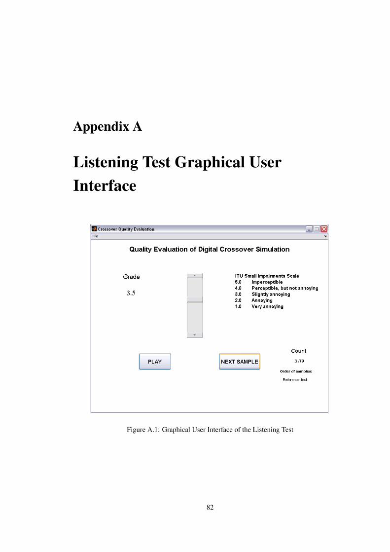
Appendix A
Listening Test Graphical UserInterface
Figure A.1: Graphical User Interface of the Listening Test
82
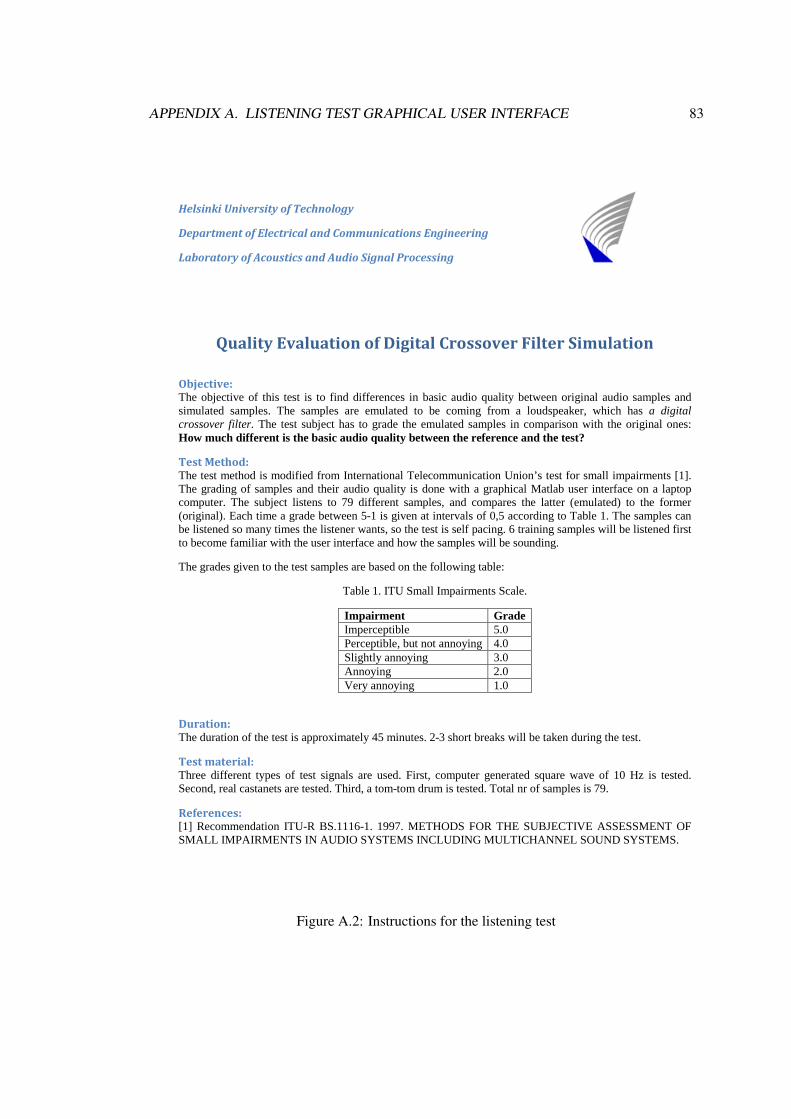
APPENDIX A. LISTENING TEST GRAPHICAL USER INTERFACE 83
Helsinki University of Technology
Department of Electrical and Communications Engineering
Laboratory of Acoustics and Audio Signal Processing
Quality Evaluation of Digital Crossover Filter Simulation
Objective: The objective of this test is to find differences in basic audio quality between original audio samples and simulated samples. The samples are emulated to be coming from a loudspeaker, which has a digital crossover filter. The test subject has to grade the emulated samples in comparison with the original ones: How much different is the basic audio quality between the reference and the test?
Test Method: The test method is modified from International Telecommunication Union’s test for small impairments [1]. The grading of samples and their audio quality is done with a graphical Matlab user interface on a laptop computer. The subject listens to 79 different samples, and compares the latter (emulated) to the former (original). Each time a grade between 5-1 is given at intervals of 0,5 according to Table 1. The samples can be listened so many times the listener wants, so the test is self pacing. 6 training samples will be listened first to become familiar with the user interface and how the samples will be sounding.
The grades given to the test samples are based on the following table:
Table 1. ITU Small Impairments Scale.
Impairment Grade Imperceptible 5.0 Perceptible, but not annoying 4.0 Slightly annoying 3.0 Annoying 2.0 Very annoying 1.0
Duration: The duration of the test is approximately 45 minutes. 2-3 short breaks will be taken during the test.
Test material: Three different types of test signals are used. First, computer generated square wave of 10 Hz is tested. Second, real castanets are tested. Third, a tom-tom drum is tested. Total nr of samples is 79.
References: [1] Recommendation ITU-R BS.1116-1. 1997. METHODS FOR THE SUBJECTIVE ASSESSMENT OF SMALL IMPAIRMENTS IN AUDIO SYSTEMS INCLUDING MULTICHANNEL SOUND SYSTEMS.
Figure A.2: Instructions for the listening test

Appendix B
Results of the listening test
2000 100001
2
3
4
5
Gra
de
Order
FIR crossover at 100 Hz with 0,5 ms delay, square wave
700 100001
2
3
4
5G
rade
Order
FIR crossover at 100 Hz with 0,5 ms delay, castanets
700 100001
2
3
4
5
Gra
de
Order
FIR crossover at 100 Hz with 0,5 ms delay, tomtom
0 0,1 0,2 0,3 0,51
2
3
4
5
Gra
de
Delay [ms]
FIR 1000th order crossover at 1 kHz, square wave
0,1 0,2 0,31
2
3
4
5
Gra
de
Delay [ms]
FIR 2000th order crossover at 1 kHz, castanets
0,51
2
3
4
5
Gra
de
Delay [ms]
FIR 2000th order crossover at 1 kHz with 0,5 ms delay, tomtom
Figure B.1: Results of the listening test for FIR crossovers.
84
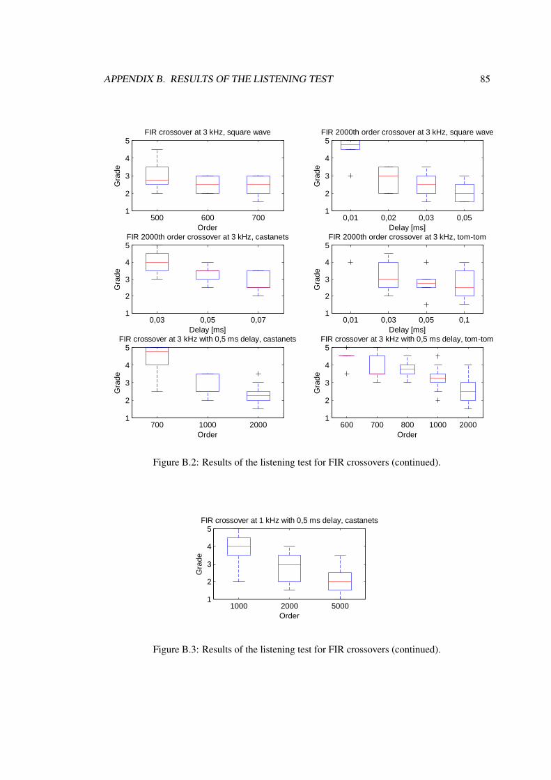
APPENDIX B. RESULTS OF THE LISTENING TEST 85
500 600 7001
2
3
4
5
Gra
de
Order
FIR crossover at 3 kHz, square wave
0,01 0,02 0,03 0,051
2
3
4
5
Gra
de
Delay [ms]
FIR 2000th order crossover at 3 kHz, square wave
0,03 0,05 0,071
2
3
4
5
Gra
de
Delay [ms]
FIR 2000th order crossover at 3 kHz, castanets
0,01 0,03 0,05 0,11
2
3
4
5
Gra
de
Delay [ms]
FIR 2000th order crossover at 3 kHz, tomtom
700 1000 20001
2
3
4
5
Gra
de
Order
FIR crossover at 3 kHz with 0,5 ms delay, castanets
600 700 800 1000 20001
2
3
4
5
Gra
de
Order
FIR crossover at 3 kHz with 0,5 ms delay, tomtom
Figure B.2: Results of the listening test for FIR crossovers (continued).
1000 2000 50001
2
3
4
5
Gra
de
Order
FIR crossover at 1 kHz with 0,5 ms delay, castanets
Figure B.3: Results of the listening test for FIR crossovers (continued).
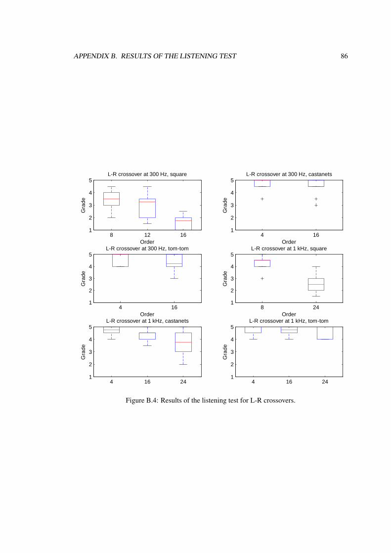
APPENDIX B. RESULTS OF THE LISTENING TEST 86
8 12 161
2
3
4
5
Gra
de
Order
LR crossover at 300 Hz, square
4 161
2
3
4
5
Gra
de
Order
LR crossover at 300 Hz, castanets
4 161
2
3
4
5
Gra
de
Order
LR crossover at 300 Hz, tomtom
8 241
2
3
4
5
Gra
de
Order
LR crossover at 1 kHz, square
4 16 241
2
3
4
5
Gra
de
Order
LR crossover at 1 kHz, castanets
4 16 241
2
3
4
5
Gra
de
Order
LR crossover at 1 kHz, tomtom
Figure B.4: Results of the listening test for L-R crossovers.
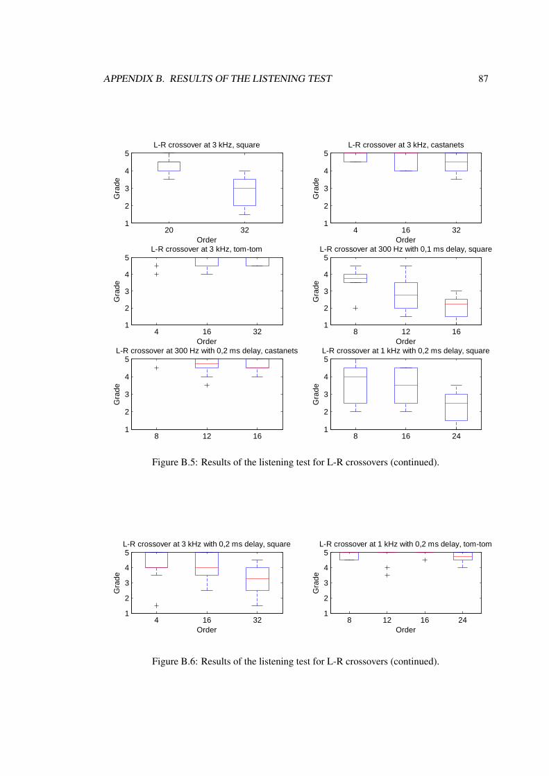
APPENDIX B. RESULTS OF THE LISTENING TEST 87
20 321
2
3
4
5
Gra
de
Order
LR crossover at 3 kHz, square
4 16 321
2
3
4
5
Gra
de
Order
LR crossover at 3 kHz, castanets
4 16 321
2
3
4
5
Gra
de
Order
LR crossover at 3 kHz, tomtom
8 12 161
2
3
4
5
Gra
de
Order
LR crossover at 300 Hz with 0,1 ms delay, square
8 12 161
2
3
4
5
Gra
de
Order
LR crossover at 300 Hz with 0,2 ms delay, castanets
8 16 241
2
3
4
5
Gra
de
Order
LR crossover at 1 kHz with 0,2 ms delay, square
Figure B.5: Results of the listening test for L-R crossovers (continued).
4 16 321
2
3
4
5
Gra
de
Order
LR crossover at 3 kHz with 0,2 ms delay, square
8 12 16 241
2
3
4
5
Gra
de
Order
LR crossover at 1 kHz with 0,2 ms delay, tomtom
Figure B.6: Results of the listening test for L-R crossovers (continued).

Appendix C
Results of the listening test as table
Sample number Type Order Crossover Delay Signal Average GrpDel error [ms] Smoothed spectrum
29 LR 8 300 0 square 3,4 4,14 unity
21 LR 12 300 0 square 3,0 6,9 unity
2 LR 16 300 0 square 1,7 9,8 unity
20 LR 8 1000 0 square 4,4 1,25 unity
18 LR 24 1000 0 square 2,7 4,9 unity
6 LR 20 3000 0 square 4,3 1,3 unity
23 LR 32 3000 0 square 2,9 2,4 unity
16 LR 8 300 0,1 square 3,7 4,1 -0,03
22 LR 12 300 0,1 square 2,9 6,7 -0,03
30 LR 16 300 0,1 square 2,2 9,5 0,05
15 LR 8 1000 0,2 square 3,8 1,24 -1,74
8 LR 16 1000 0,2 square 3,5 2,6 -1,25
5 LR 24 1000 0,2 square 2,4 4,2 -0,95
25 LR 4 3000 0,2 square 4,0 0,85 -8,8
28 LR 16 3000 0,2 square 4,1 2,36 -3,9
19 LR 32 3000 0,2 square 3,1 4,85 -2,1
53 LR 4 300 0 kast 4,7 1,8 unity
45 LR 16 300 0 kast 4,4 9,8 unity
39 LR 4 1000 0 kast 4,7 0,54 unity
50 LR 16 1000 0 kast 4,4 3 unity
47 LR 24 1000 0 kast 3,7 4,9 unity
31 LR 4 3000 0 kast 4,9 0,18 unity
33 LR 16 3000 0 kast 4,7 1 unity
54 LR 32 3000 0 kast 4,5 2,4 unity
Figure C.1: Results of the listening test as table. Average is the average grade the sample hasreceived. GrpDel error is the deviation of group delay from a constant value. Smoothed spectrumtells the magnitude error calculated in third-octave bands.
88

APPENDIX C. RESULTS OF THE LISTENING TEST AS TABLE 89
38 LR 8 300 0,2 kast 4,9 4 -0,15
44 LR 12 300 0,2 kast 4,6 6,5 -0,13
49 LR 16 300 0,2 kast 4,6 9,3 -0,12
58 LR 4 300 0 tomtom 4,7 1,8 unity
70 LR 16 300 0 tomtom 4,4 9,8 unity
78 LR 4 1000 0 tomtom 4,8 0,54 unity
65 LR 16 1000 0 tomtom 4,7 3 unity
73 LR 24 1000 0 tomtom 4,7 4,9 unity
68 LR 4 3000 0 tomtom 4,9 0,18 unity
71 LR 16 3000 0 tomtom 4,8 1 unity
57 LR 32 3000 0 tomtom 4,9 2,4 unity
69 LR 8 1000 0,2 tomtom 4,9 1,24 -1,7
60 LR 12 1000 0,2 tomtom 4,8 1,9 -1,45
56 LR 16 1000 0,2 tomtom 5,0 2,6 -1,25
74 LR 24 1000 0,2 tomtom 4,7 4,2 -0,95
9 FIR 2000 100 0,5 square 4,5 1,6 -0,1
10 FIR 10000 100 0,5 square 4,4 0,85 -0,03
24 FIR 1000 1000 0 square 4,4 0 -0,003
17 FIR 1000 1000 0,1 square 4,4 1,15 -0,1
26 FIR 1000 1000 0,2 square 3,2 2,8 -0,45
7 FIR 1000 1000 0,3 square 2,9 4,6 -0,8
11 FIR 1000 1000 0,5 square 3,1 0,52 -1,4
13 FIR 500 3000 0,2 square 2,9 5,25 -0,75
1 FIR 600 3000 0,2 square 2,5 6,14 -0,6
14 FIR 700 3000 0,2 square 2,4 6,8 -0,5
27 FIR 2000 3000 0,01 square 4,5 0 -0,001
Figure C.2: Results of the listening test as table (continued).
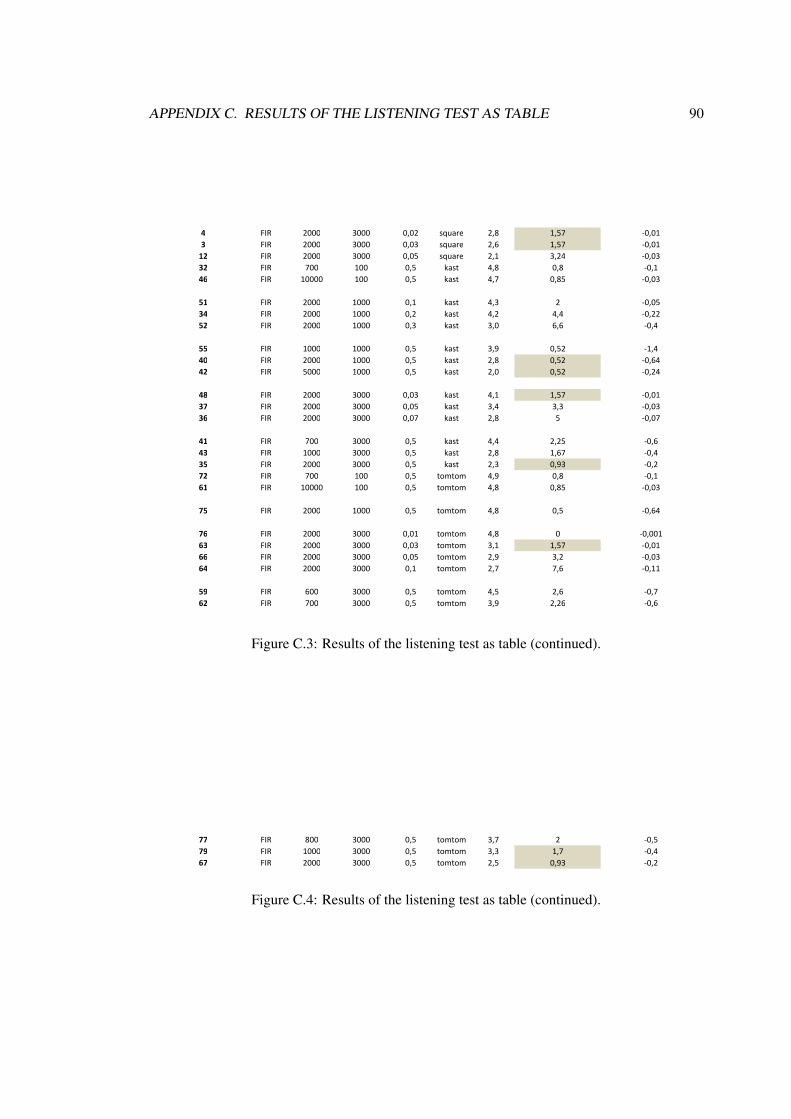
APPENDIX C. RESULTS OF THE LISTENING TEST AS TABLE 90
4 FIR 2000 3000 0,02 square 2,8 1,57 -0,01
3 FIR 2000 3000 0,03 square 2,6 1,57 -0,01
12 FIR 2000 3000 0,05 square 2,1 3,24 -0,03
32 FIR 700 100 0,5 kast 4,8 0,8 -0,1
46 FIR 10000 100 0,5 kast 4,7 0,85 -0,03
51 FIR 2000 1000 0,1 kast 4,3 2 -0,05
34 FIR 2000 1000 0,2 kast 4,2 4,4 -0,22
52 FIR 2000 1000 0,3 kast 3,0 6,6 -0,4
55 FIR 1000 1000 0,5 kast 3,9 0,52 -1,4
40 FIR 2000 1000 0,5 kast 2,8 0,52 -0,64
42 FIR 5000 1000 0,5 kast 2,0 0,52 -0,24
48 FIR 2000 3000 0,03 kast 4,1 1,57 -0,01
37 FIR 2000 3000 0,05 kast 3,4 3,3 -0,03
36 FIR 2000 3000 0,07 kast 2,8 5 -0,07
41 FIR 700 3000 0,5 kast 4,4 2,25 -0,6
43 FIR 1000 3000 0,5 kast 2,8 1,67 -0,4
35 FIR 2000 3000 0,5 kast 2,3 0,93 -0,2
72 FIR 700 100 0,5 tomtom 4,9 0,8 -0,1
61 FIR 10000 100 0,5 tomtom 4,8 0,85 -0,03
75 FIR 2000 1000 0,5 tomtom 4,8 0,5 -0,64
76 FIR 2000 3000 0,01 tomtom 4,8 0 -0,001
63 FIR 2000 3000 0,03 tomtom 3,1 1,57 -0,01
66 FIR 2000 3000 0,05 tomtom 2,9 3,2 -0,03
64 FIR 2000 3000 0,1 tomtom 2,7 7,6 -0,11
59 FIR 600 3000 0,5 tomtom 4,5 2,6 -0,7
62 FIR 700 3000 0,5 tomtom 3,9 2,26 -0,6
Figure C.3: Results of the listening test as table (continued).
77 FIR 800 3000 0,5 tomtom 3,7 2 -0,5
79 FIR 1000 3000 0,5 tomtom 3,3 1,7 -0,4
67 FIR 2000 3000 0,5 tomtom 2,5 0,93 -0,2
Figure C.4: Results of the listening test as table (continued).

Appendix D
Results of Real LoudspeakerExperiment
Lou
dsp
ea
ke
r e
xp
eri
me
nt
da
te:
28
.1,
29
.1.2
00
8
loca
tio
n:
List
en
ing
ro
om
of
Aco
ust
ics
Lab
ora
tory
at
He
lsin
ki
Un
ive
rsit
y o
f T
ech
no
log
y
sub
ject
1su
bje
ct2
sub
ject
3su
bje
ct4
sub
ject
5
10
Hz
squ
are
wa
ve
sitt
ing
sta
nd
ing
sitt
ing
sta
nd
ing
sitt
ing
sta
nd
ing
sitt
ing
sta
nd
ing
sitt
ing
sta
nd
ing
po
siti
on
11
50
02
00
09
00
15
00
12
00
24
00
60
09
00
90
02
00
0
po
siti
on
22
00
02
00
09
00
12
00
90
09
00
60
09
00
90
01
50
0
po
siti
on
32
00
02
00
02
00
02
40
02
40
02
00
01
20
09
00
90
01
50
0
po
siti
on
42
00
02
00
01
20
09
00
12
00
90
09
00
60
01
20
01
20
0
po
siti
on
56
00
24
00
60
01
20
06
00
15
00
60
06
00
60
01
50
0
the
ca
sta
ne
tssi
ttin
gst
an
din
gsi
ttin
gst
an
din
gsi
ttin
gst
an
din
gsi
ttin
gst
an
din
gsi
ttin
gst
an
din
g
po
siti
on
11
20
01
50
01
20
01
50
01
20
01
20
09
00
15
00
15
00
20
00
po
siti
on
11
20
01
50
01
20
01
50
01
20
01
20
09
00
15
00
15
00
20
00
po
siti
on
22
00
02
40
01
20
02
00
09
00
12
00
12
00
12
00
15
00
12
00
po
siti
on
32
00
02
40
02
40
01
50
02
40
02
00
01
20
01
20
02
00
02
00
0
po
siti
on
42
40
01
50
01
20
01
50
01
20
01
50
01
20
01
20
02
00
02
00
0
po
siti
on
59
00
24
00
90
02
00
09
00
24
00
90
01
20
01
20
02
40
0
Figure D.1: Results of the real loudspeaker experiment in a listening room.
91