Embed Size (px)
Citation preview

Loudspeaker crossover networks
ØrstedDTU – Acoustical Technology 1
Loudspeaker crossover networks
By
Tore A. Nielsen
Student 041915 at DTU, the Technical University of Denmark
August 2005
Abstract
Loudspeaker systems use crossover networks directing low and high frequencies to individual loudspeaker units optimised for limited frequency ranges. The introduction of a crossover network should not degrade the resultant performance but the loudspeakers are physically separated, which introduces problems around the crossover frequency when listening off-axis, and the individual responses of the loudspeaker units further complicates summation of the output signals. The front baffle introduces reflections from the edges and the listening room adds reflections from its boundaries causing interference with the direct signal seriously affecting the resultant response of the loudspeaker system.
The objective of this report is the study of crossover networks and the different causes that degrades the performance.
Loudspeaker crossover networks
ØrstedDTU – Acoustical Technology 2
Contents
1. Introduction ........................................................................................................... 5
1.1. Crossover network .......................................................................................... 5
1.2. Threshold of hearing ....................................................................................... 6
1.2.1. Audible range .......................................................................................... 6
1.2.2. Change of level ........................................................................................ 6
1.2.3. Group delay ............................................................................................. 7
1.3. Musical instruments ........................................................................................ 7
1.4. Cut-off slope ................................................................................................... 8
1.5. Transfer function ............................................................................................ 9
1.5.1. Ideal filters – Constant voltage filters ..................................................... 10
1.5.2. Non-ideal filters – All-pass filters .......................................................... 11
1.5.3. Butterworth filters .................................................................................. 13
2. Crossover networks ............................................................................................. 15
2.1. First-order ..................................................................................................... 15
2.1.1. Symmetrical – two way ......................................................................... 15
2.1.2. Using bass loudspeaker roll-off .............................................................. 17
2.2. Second-order ................................................................................................ 19
2.2.1. Asymmetrical – two way ....................................................................... 19
2.2.2. Symmetrical – two way ......................................................................... 21
2.2.3. Symmetrical – three way........................................................................ 22
2.2.4. Steep cut-off – two way ......................................................................... 24
2.3. Third order.................................................................................................... 27
2.3.1. Asymmetrical – two way ....................................................................... 27
2.3.2. Symmetrical – two way ......................................................................... 29
2.3.3. Symmetrical – three way........................................................................ 30
2.3.4. Steep cut-off – two way ......................................................................... 31
2.4. Fourth order .................................................................................................. 34
2.4.1. Symmetrical – three way........................................................................ 34
2.4.2. Steep cut-off – two way ......................................................................... 35
2.5. Passive network ............................................................................................ 37
2.5.1. First order .............................................................................................. 37
2.5.2. Second order .......................................................................................... 38
2.5.3. Third order ............................................................................................ 38
2.5.4. Fourth order ........................................................................................... 39
2.5.5. Loudspeaker impedance ......................................................................... 40
2.6. Active network ............................................................................................. 42
2.6.1. First order .............................................................................................. 43
2.6.2. Second order .......................................................................................... 43
2.6.3. Higher orders ......................................................................................... 43
2.6.4. Special ................................................................................................... 44
3. Models ................................................................................................................ 46
3.1. Electro-acoustical model ............................................................................... 46
3.1.1. The loudspeaker unit .............................................................................. 47
3.1.2. Electrical circuit ..................................................................................... 49
3.1.3. Mechanical circuit ................................................................................. 50
3.1.4. Acoustical circuit ................................................................................... 52

Loudspeaker crossover networks
ØrstedDTU – Acoustical Technology 3
3.1.5. Diaphragm velocity ............................................................................... 54
3.1.6. Sound pressure ...................................................................................... 57
3.2. Loudspeaker pass band ................................................................................. 59
3.2.1. Sound pressure level .............................................................................. 59
3.2.2. Diaphragm excursion ............................................................................. 60
3.2.3. SPICE simulation model ........................................................................ 61
3.3. Directivity .................................................................................................... 62
3.4. Diffraction .................................................................................................... 63
3.4.1. Circular baffle ........................................................................................ 63
3.4.2. Sectional baffle ...................................................................................... 65
3.4.3. Square baffle ......................................................................................... 66
3.5. Listening angle ............................................................................................. 69
3.5.1. Two loudspeakers .................................................................................. 69
3.5.2. Three loudspeakers ................................................................................ 71
3.6. Boundary reflection ...................................................................................... 73
3.6.1. One reflecting surface ............................................................................ 73
3.6.2. Rectangular room .................................................................................. 75
3.6.3. Home entertainment ............................................................................... 77
3.6.4. Public address ........................................................................................ 80
3.7. Loudspeaker characteristics .......................................................................... 81
3.8. Group delay .................................................................................................. 82
3.8.1. Calculation method ................................................................................ 82
3.8.2. Implementation in MATLAB ................................................................. 82
3.8.3. Verification............................................................................................ 83
4. Assembling the models ....................................................................................... 86
4.1. Loudspeaker models ..................................................................................... 86
4.2. Crossover network ........................................................................................ 86
4.3. Angular response .......................................................................................... 89
4.4. Reflections .................................................................................................... 90
4.5. Conclusion .................................................................................................... 91
5. References .......................................................................................................... 92
5.1. Books ........................................................................................................... 92
5.2. Papers ........................................................................................................... 92
5.3. Links ............................................................................................................ 92
6. Appendix ............................................................................................................ 93
6.1. Plot transfer function .................................................................................... 93
6.1.1. Main script ............................................................................................ 93
6.1.2. Filter function ........................................................................................ 96
6.1.3. Loudspeaker .......................................................................................... 96
6.1.4. Directivity ............................................................................................. 97
6.1.5. Diffraction ............................................................................................. 97
6.1.6. Boundary reflections .............................................................................. 97
6.2. Plot boundary reflection ................................................................................ 98

Loudspeaker crossover networks
ØrstedDTU – Acoustical Technology 4
Foreword
The current project was initiated as a three-week course to be executed in August of the 2005 summer vacation since I could not participate in the normal three-week period in June. My professor Finn Agerkvist accepted the proposal of a project to study crossover networks.
The main objective was the design of crossover networks realising a transfer function of unity, i.e. flat amplitude and zero phase, and I planned to include the effect of loudspeaker bandwidth, the problems associated with off-axis listening due to the displacement of the loudspeaker on the front baffle and the interference from reflections within the listening room. Finn Agerkvist suggested that I also included the reflections due to diffraction.
Initially I planned to use SPICE for simulations and a spread sheet for calculations, but I soon realised that it was more appropriate to base the simulations and calculations on MATLAB.
I decided to work through the loudspeaker model presented by Leach in order to derive a useful model for loudspeakers, and I included the effect of the voice coil inductance and combined the low and high frequency models from Leach into one single model, which covers the frequency range below diaphragm break-up.
As the project progressed, I realised the need to include group delay and it seemed appropriate to add notes on the threshold of hearing thus defining an acceptance limit for use during the development of a crossover network.
According to my log, I have been working for 180 hours, which is 50 % more than the nominal workload for a three-week course. If an unlimited amount of time were available, I would have worked more on high-order crossover filters and improved the sections on diffraction, off-axis listening, boundary reflection and group delay.
Tore A. Nielsen
August 14, 2005.
Loudspeaker crossover networks
ØrstedDTU – Acoustical Technology 5
1. Introduction Ideally, a single loudspeaker should reproduce the full audible frequency range without any detectable distortion, but this is unfortunately not possible although good full-range loudspeakers do exist. The frequency range of a full-range loudspeaker is limited with weak bass and unsatisfactory treble, the frequency response is irregular or at least compromised by the directivity at high frequencies and it is difficult to keep distortion low when the same diaphragm is used for bass and treble.
Low frequencies moves the diaphragm significantly at high sound pressure levels thus introducing harmonic distortion related to loudspeaker construction (magnet, voice coil and suspension) and inter-modulation between bas and treble caused by the Doppler-effect. The one and only way of distortion reduction is decreasing diaphragm excursion, but this require an increase of diaphragm area to compensate for the lost sound pressure; and enlarging loudspeaker size worsens high frequency reproduction.
It all boils down to a requirement of loudspeakers optimised for reproduction of a limited frequency range and thus the need of a frequency dividing network.
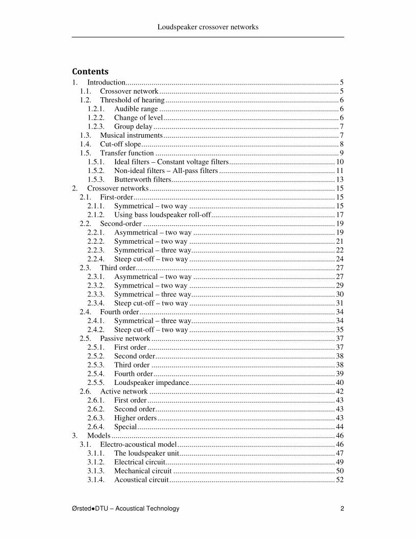
1.1. Crossover network
A pair of typical crossover networks are shown in Figure 1. To the left is a two-way system, which could use a crossover frequency around 2 kHz, and to the right is a three-way system, which could use crossover frequencies around 800 Hz and 4 kHz.
High-pass
filter
Low-pass filter
High-pass
filter
Band-pass filter
Low-pass filter
High-frequency loudspeaker
(Treble)
Mid-frequency loudspeaker
(Midrange)
Low-frequency loudspeaker
(Bass)
PA
PA
PA
PA
Audio
source
Audio
source
Figure 1 – Layout of a typical cross-over network, which can be passive, i.e. consisting
of capacitors, inductors and resistors and driven from a single power amplifier (left),
or it can be active, i.e. using operational amplifiers with frequency-dependent
feedback and individual power amplifiers for each channel (right).
The loudspeakers are driven from power amplifiers, which can either be located before the crossover network; the conventional approach using passive crossover networks, or the power amplifier can be located between the crossover network and the loudspeaker; thus requiring an amplifier for each loudspeaker.
The passive crossover network is currently the most used approach but the active crossover network is expected to be increasingly popular in the near future since high-quality power amplifier modules based upon the switch-mode technique (Class D) are becoming a serious alternative to the linear power amplifiers of today. In addition to improved control of filter parameters and protection of the loudspeakers do the active crossover network offer electrical control of the moving system parameters and adjustment of the response to the listening room.
But before entering the study of crossover networks, a few words on what can be heard, and what cannot, is required.

Loudspeaker crossover networks
ØrstedDTU – Acoustical Technology 6
1.2. Threshold of hearing
There is no idea in optimising a filter if the improvement is inaudible and the money could be spend better on other jobs. So, here is a brief overview of what is audible and what is not. Don’t take the limits too literately; they are meant as guidelines.
1.2.1. Audible range
The audible range is defined by the Fletcher-Munson curves reproduced to the left in Figure 2. They published their data in 1933 using headphones; measurements using anechoic chambers were published in 1956 by Robinson-Dadson and later reviewed and standardised in 2003 as ISO 226, shown to the right.
Figure 2 – Equal loudness contours due to Fletcher-Munson (http://en.wikipedia.org)
and to Robinson-Dadson (http://www.aist.go.jp/aist_e/latest_research).
We can hear signals from 15 Hz to 15 kHz but few loudspeaker systems can reproduce this range, at least not at realistic levels since low-frequency signals require large diaphragms and long voice coils in order to move the air; the sound pressure level must exceed 80 dB at very low frequencies to be heard and 110 dB is required at 20 Hz to balance a typical speech level around 65 dB.
Organ music may extend to 16 Hz for organs fitted with 32 feet pipes, but they are rarely found – and rarely used – so organs music is limited to 32 Hz. Piano music may extend to 27 Hz, while jazz, rock and popular music seldom passes below 41 Hz; the lowest string on the acoustical double bass and the electric bass guitar. Powerful low-frequency signals may, however, arise from electrical keyboards, computerized effects and recordings of large drums, machines, thunder storms and explosions.
No one can hear sound above 20 kHz, and aging further reduces the limit, so a pragmatic upper limit would be 15 kHz. People with “golden ears” may postulate that the treble unit should extend far beyond 20 kHz to avoid phase distortion. The audibility of phase is controversial, so a safe view would be that reproduction beyond 20 kHz do not harm; but have in mind that FM-radio broadcasting limits the range to 15 kHz and CD-recordings to 20 kHz. Modern signal transmission using MPEG and other formats often use the 44.1 kHz sampling frequency of the CD-media thus sharing the limit.
1.2.2. Change of level
The ability to detect a change of level is between 0.5 dB and 2 dB [1] so loudspeaker artefacts below this limit can be expected inaudible. This is quite fortunate, since

Loudspeaker crossover networks
ØrstedDTU – Acoustical Technology 7
irregularities of this order of magnitude must be expected with loudspeakers. It is obvious that the lowest limit should be used designing high-end equipment, since the listener can be expected to have trained ears.
1.2.3. Group delay
Threshold of audibility of group delay is being debated, but it should be relatively safe stating the limit as a couple of milliseconds for signals in the 500 Hz to 8 kHz range. (Source: http://www.trueaudio.com/post_010.htm).
1.3. Musical instruments
The fundamental note of musical instruments is typical located below 1 kHz as shown in Figure 3. The harmonic overtones extend beyond the hearing limit but the level is reduced toward the higher frequencies. The decay is strongly dependent upon the actual instrument being examined, but an average slope would be around –6 dB/octave. Most music use fundamentals within the 3½ octave range from the lower C-note at 65 Hz to the upper g2-note at 780 Hz, so the musical power is mainly restricted to this range.
10 Hz 100 Hz 1 kHz 10 kHz
String quartet
Human voice
Brass ensemble
Wood wind
Piano
Organ
Orchester
Dynamic range
50 dB
50 dB
35 dB35 dB
70 dB
50 dB
50 dB
Figure 3 – Frequency range for the fundamental note of musical instruments [5].
The dynamic range extend from 40 dB to 110 dB for acoustical instruments and higher for electrically amplified music. A symphony or rock orchestra cannot be reproduced at realistic levels for home entertainment, so the playback level must typically be reduced.
Recording level was previously compressed manually by increasing the weakest levels during recording, in order to cut the master disk (LP records) keeping the weakest signals above the noise floor of the medium. This is not needed nowadays for recording of compact disks (CD), where the dynamic level is, at least theoretically, 96 dB.
Reducing the reproduction level moves the weakest signals below the threshold of hearing, at least for the lowest frequencies, so the loudspeaker system may require a bass boost for reproduction at reduced levels. This is sometimes called physiological
loudness contour and is included with many amplifier systems. The success of this correction is dependent upon the set-up of the combined system, consisting of the source, the amplifier, the loudspeaker and the size of the room and is most effectively implemented with integrated systems where the interconnection levels are known.
The correction is often accompanied by a treble boost as well, but this is based on a misinterpretation of the equal loudness contour; the treble part of the equal loudness contour is turned upward at high frequency thus indicating reduced sensitivity at high frequencies, but the distance between the different levels is almost constant so correction is not required.

Loudspeaker crossover networks
ØrstedDTU – Acoustical Technology 8
1.4. Cut-off slope
A crossover network is not a brick wall filter with infinite attenuation outside the pass band; the crossover network gradually attenuates the signal above or below the crossover frequency as illustrated in Figure 4 for low-pass and high-pass filters.
The pass band is the frequency range where attenuation is minimum, typically –3 dB although some filters attenuate more than this. The transition band is the frequency range where the attenuation is becoming active and the stop band is the frequency range where the attenuation has become sufficient to efficiently remove the loudspeaker.
Figure 4 – Filter characteristics for Butterworth filters with orders 1, 2, 3, 4 and 6.
A loudspeaker contributes with audible output in the transition band, which must be taken into account to avoid interference between the loudspeakers. Sufficient amount of attenuation is obtained when the level from the attenuated channel is less than a certain limit, for instance below –20 dB. The limit defines the acceptable interference level.
Assume for example, that the loudspeaker peaks 6 dB at some frequency near the stop band and that this must be attenuated. With –20 dB of intended attenuation this corresponds an actual level of –14 dB, or a sound pressure of 10-14/20 = 20 % of the nominal level, which may result in ±2 dB of interference.
A crossover network with a cut-off slope of ±6 dB/octave indicates that the loudspeaker must be well-behaved for at least 3 octaves beyond the cross-over frequency. A bass loudspeaker, which is to be cut-out above 2 kHz, must be reasonably flat to 16 kHz.
The crossover network must protect the treble loudspeaker from the high power levels at lower frequencies. The loudspeaker is compliance-controlled below the resonance frequency, which is usually around 1 kHz, so the diaphragm moves in proportion to the applied voltage. The low-frequency excursion of the diaphragm may be inaudible but it may give rise to audible distortion of high-frequency signals when the low-frequency excursion of the suspension system reaches the non-linear region. The unnecessary dissipation of power heats the voice coil and may damage the treble loudspeaker, which is capable of handling few watts only.
Most of the signal power in music is located below approximately 500 Hz so a power reduction well below 1 W of dissipation within the treble loudspeaker requires in excess of 20 dB of attenuation for sufficient protection. If the treble loudspeaker is to be cut-in at 2 kHz, which is just two octaves above 500 Hz, the required filter slope becomes a minimum of 12 dB/octave.

Loudspeaker crossover networks
ØrstedDTU – Acoustical Technology 9
1.5. Transfer function
All channels of the crossover network will be described by their transfer function, which is a convenient way of describing an electrical filter, and system analogies allow straightforward transformation to mechanical and acoustical systems as well. The transfer function may be defined from requirements such as flat amplitude, which can then be used to specify the system parameters.
Bandwidth-limited channel #1
H1
Input
signal
Bandwidth-limited
channel #2
H2
+
+
Output
signal
EOUT = (H1 + H2)EIN EIN
EOUT1 = H1EIN
EOUT2 = H2EIN
Σ
Figure 5 – A crossover network consists of two or more filter channels dividing the
frequency range between the loudspeakers. The output from the loudspeakers are
summed at the observation point; i.e. at the ear of the listener.
Transfer functions will be expressed in the frequency domain where frequency is
represented by the Laplace operator s, defined by: s = α + iω. The initial conditions are
described by α and ω = 2πf is the angular frequency. Throughout this report is α = 0, so
s = iω can be assumed although the formulas are generally valid and may, if required, be transformed to the time domain using the inverse Laplace transform. However, time domain representations are not referenced in this document.
The complex frequency operator will be normalised by division with ω0, which represents the cut-off frequency in most situations.
0
0 ωs
s =
A transfer function H is defined by the excitation input to the network, EIN, and the output response from the network, EOUT. Assuming sinusoidal excitation:
( )tiHEHEE INOUT ωexp0==
An input excitation signal EIN is routed in parallel to the channels of a network with the individual transfer functions H1, H2, ... and the output signals become:
...,, 2211 INOUTINOUT EHEEHE ==
The loudspeakers will, for the moment, be considered ideal, so the acoustical output of the loudspeaker is a true copy of the electrical input signal. Assuming linearity, the signals from the individual channels are added at the receiver:
K++= 21 OUTOUTOUT EEE
Using the above definition of the transfer function, the sum can be written:
( ) INMOUT EHHHE +++= K21
The sum of the individual transfer functions is defined as the system transfer function.
MHHHH K++= 21

Loudspeaker crossover networks
ØrstedDTU – Acoustical Technology 10
The main objective of this report is analysing the system transfer function for the complete system involving the crossover network, the loudspeakers, the front baffle and the listening room. In order to do so, a reference transfer function is needed for comparison. It is obvious, that an ideal transfer function should not add or remove any information, it should be a string of wire.
1=H
A scaling factor, different from unity, is allowed, since amplification, attenuation, sign inversion or time delay within the system is not considered a distortion of the signal. The scaling factor may also include a dimension for transformation between the electrical, mechanical or acoustical systems.
1.5.1. Ideal filters – Constant voltage filters
Although loudspeakers are far from ideal, avoiding approximations in the design of the crossover network it is a good starting point. The design of crossover networks fulfilling the requirement H = 1, which guarantees flat amplitude and a phase of zero, are called constant-voltage filters and will be based upon the following polynomial:
NN
NN ssasasaP 0
1
01
2
02011 +++++= −−L
The constants a1, a2, …, aN-1 defines the filter type, N is the order of the polynomial and the coefficients are shown for the Butterworth filter type later in this chapter.
Other polynomials, such as Bessel or Chebychev, can use the above polynomial form if they are normalised to unity for coefficients a0 and aN. If this is not the case, all terms of the
polynomials must be divided by a0, and the normalisation coefficient ω0 must thereafter be corrected to include a0 and aN.
An alternative representation of PN is the product form, which is using the roots of the polynomial.
The third order Butterworth polynomial can be represented by the following two identical expressions:
( ) ( ) ( )0003
3
0
2
003
866.05.0866.05.01
221
sisisP
sssP
+−×++×+=+++=
After the multiplications are carried out the original polynomial results.
A transfer function of order N can now be defined:
N
o
N
N
N
o
N
N
N
NN
ssasasa
ssbsbsb
P
QH
++++++++++
== −−
−−
1
01
2
0201
1
01
2
0201
1
1
L
L
The transfer function satisfy the requirement H = 1 when ai = bi since the nominator polynomial QN and denominator polynomial PN are identical, but the requirement will
be violated, if ai ≠ bi for one or more of the terms. This violation may be required building crossover networks of high order where the ideal transfer function becomes cumbersome. The result is anyway a valid transfer function although the phase response and possibly also the amplitude response will be affected.

Loudspeaker crossover networks
ØrstedDTU – Acoustical Technology 11
Division into crossover channels uses the following identity:
N
N
N
N
N
NNN
NP
s
P
sb
P
sb
P
sb
PH 0
1
01
2
02011+++++=
−−
L
Each term represents a transfer function with its own characteristics and two or more terms can be combined as required. All terms share the same denominator polynomial and are thus of the same order, regardless of the actual order of the nominator.
Two examples will introduce the method.
Example 1. For a first-order crossover only two terms are available so the design leaves no choice other than accepting the following arrangement:
0
0
1
01
0
111
11
s
s
P
sH
sPH HP
N
LP +==
+==
Example 2. For a crossover network of sufficiently high order (N ≥ 4), the first two terms of PN can be used for the bass channel, the last two terms for the treble channel and the remaining terms are available for the midrange channel:
N
NN
N
HPN
N
N
N
BPN
N
LPNP
ssbH
P
sbsbH
P
sbH 0
1
01
2
02
2
02011 +=
++=
+=
−−
−−L
The cut-off slopes are proportional to 1/fN-1 for the bass channel, fN-1 for the treble channel and f2 and 1/f2 for the midrange channel. A fourth order filter would offer cut-off slopes of ±18 dB/octave for bass and treble and ±12 dB/octave for midrange.
Both filters are realised in the next chapter together with other implementations.
1.5.2. Non-ideal filters – All-pass filters
The above method is useful for filters up to fourth order but become cumbersome for higher orders. A solution is to remove all middle terms and use only the first and last terms representing the low-pass and high-pass channels. These filters, which are called all-pass filters, can be used for crossover networks of any order. The requirement H = 1 is not satisfied so the phase of the filter will be different from zero.
With b1, b2, … , bN-1 set to zero the transfer functions become:
N
N
N
N
N
HPN
N
LPNP
sH
P
sHand
PH 00 11 +
=⇒==
The first term represents a low-pass channel with a cut-off frequency of f0 = ω0/2π and a cut-off slope of 1/fN, so the higher frequencies are attenuated by –6N dB/octave. Filter amplitude response is flat under certain conditions, which will be analysed below. First-order filters are ideal (constant-voltage filters) and will not need special considerations.
Ns
N
s
N
LPN
sP
PH
0
0
11
11
0
0
→=
→=
∞→
→
The second term represents a high-pass channel with a cut-off frequency of f0 = ω0/2π and a cut-off slope of fN, so the lower frequencies are attenuated by 6N dB/octave.
Frequency
Amplitude
f0
-6N dB/octave 1

Loudspeaker crossover networks
ØrstedDTU – Acoustical Technology 12
10
00
00
0
0
0
= →=
→=
∞→
→
N
N
s
N
N
N
s
N
N
HPN
s
s
P
s
sP
sH
When the output from both channels are combined the following transfer function for the complete system is obtained:
N
N
N
N
N
NP
iHcrossoverAt
P
sH
+=
+=
1:
1 0
At crossover (s0 = i) is the sum depending upon the filter order and for N = 2, 6, 10, ... the terms cancel – no signal is being transmitted at crossover. The cancellation can be avoided by sign inversion one of the channels, which has the consequence that the phase moves from 0° to –180° through the frequency range.
• For N odd are the channels 90° or 270° out of phase, and the channels combine at crossover with 3 dB of loss. To avoid peaking, the transfer functions must be designed to –3 dB at the crossover frequency and this can be realised using a Butterworth polynomial as basis for the design.
• For N even are two channels in-phase if the above mentioned sign inversion is included as required and the channels combine at crossover without loss. To avoid peaking, the transfer functions must be designed to –6 dB at the crossover frequency. This can be realised using a squared Butterworth polynomial as basis for the design; a design method referred to as the Linkwitz-Riley filter design.
Constant amplitude, |HN| = 1, is realised by the so-called all-pass filters, which are based upon the Butterworth polynomials.
First-order crossover networks are born as ideal filters (i.e. constant voltage), so the
amplitude is constant. This will be demonstrated below using variable w = ω/ω0 as a substitute for s0 in order to identify real and imaginary parts of the frequency variable. The all-pass variant of the first-order crossover network (1 – s0 in the nominator) is also useful and is analysed as well [2].
11
1
1
1
1
1
22
22
0
01 =
+
+=
+±
=+±
=w
w
iw
iw
s
sH
Filters of higher order can realise the all-pass function when the polynomial used is of Butterworth characteristic, since this allows factorisation of the nominator and denominator polynomials.
Second-order crossover networks require inversion of the high-pass channel to avoid the notch filter and the level must be –6 dB at crossover, so the crossover network is based on a squared first-order Butterworth polynomial. The amplitude response becomes [2]:
( )( )( )( )( ) 1
1
1
1
1
1
1
11
11
1
1
22
22
0
0
00
00
2
0
2
02 =
+
+=
+−
=+−
=++−+
=+−
=w
w
iw
iw
s
s
ss
ss
s
sH
Frequency
Amplitude
f0
6N dB/octave 1

Loudspeaker crossover networks
ØrstedDTU – Acoustical Technology 13
Third-order crossover networks are insensitive to the sign of the treble channel (the amplitude response is unaltered although the phase response is changed). The third-order Butterworth polynomial use a1 = a2 = 2, and the factorisation results in [2]:
( )( )( )( )
( )( )
( )( )( )( ) 1
1
1
1
1
11
11
221
1
11
1
1
1
11
11
221
1
22
22
2
000
2
000
3
0
2
00
3
03
22
222
2
2
2
000
2
000
3
0
2
00
3
03
=+
+=
+−
=+++++−
=+++
−=
=+−
+−=
−+−−
=++++−+
=+++
+=
w
w
iw
iw
sss
sss
sss
sH
ww
ww
wiw
wiw
sss
sss
sss
sH
Fourth-order crossover networks require a level of –6 dB at crossover and can be based
upon a squared second-order Butterworth polynomial (a1 = √2). The amplitude response becomes [2]:
( )( )( )
( )( )( )
1
1
1
21
21
21
21
21
2121
21
1
22
22
2
2
2
00
2
00
22
00
2
00
2
00
22
00
4
04
=+
+=
+++−
=
+++−
=++
+−++=
++
+=
w
w
wwi
wwi
ss
ss
ss
ssss
ss
sH
Higher order filters are not covered in this report but can, according to reference [2], be
shown to fulfil the all-pass filter requirement H = 1.
1.5.3. Butterworth filters
Crossover networks are often based upon the Butterworth polynomial since this leads to good all-pass filters. The amplitude response for a Butterworth low-pass filter is [5]:
1
1
1
1
1
0
0
2
0
2
0
0
0
→
→
+
=+
=
→
∞→
s
N
sNNLPN
sH
ωω
ωω
The amplitude approaches unity for zero frequency, the amplitude is 1/√2 or –3 dB at the crossover frequency regardless of the filter order, and the asymptotic cut-off slope for higher frequencies is –6N dB/octave. This is a maximally flat filter and one of its characteristics is, that all filter blocks of the physical implementation will be designed for the same cut-off frequency but with different quality factors.
Other filter characteristics are realised through frequency transformation, introduced briefly below [5], but the transformations are not required for the current analysis since the different channels are generated directly from the transfer function and not from transformation of a model filter.

Loudspeaker crossover networks
ØrstedDTU – Acoustical Technology 14
A high-pass filter is realised by transformation of s0 into 1/s0:
N
s
sNNHPN
s
Hs
s
→
→
+
=
+
=⇒→
→
∞→
0
0
2
0
2
0
0
0
0
01
1
1
11
11
ωω
ωω
A band-pass filter is realised by the following transformation, which consists of 1/s0 as well as s0 in combination with a coefficient B, representing the bandwidth of the resulting filter:
N
N
Ns
is
N
N
NsNBPN
B
Bs
B
B
s
Bs
s
HBs
ss
=
→
→
=
→
++
=⇒+
→
→
=
∞→
0
0
0
0
02
0
2
00
2
00
1
1
1
1
11
11
0
0
0
ωω
ωω
The coefficients and roots of the Butterworth polynomial is shown in the table below for filters from second to seventh order. The first-order polynomial 1 + s0 is Butterworth too but do not include coefficients to be defined.
Table 1 – Coefficients and roots of Butterworth polynomials (from [5]).
Order Coefficients Roots
2 a1 = 1.4142 (-0.7071 ±i0.7071)
3 a1 = a2 = 2.0000 (-1)
(-0.5000 ±i0.8660)
4 a1 = a3 = 2.6131
a2 = 3.4142 (-0.3827 ±i0.9239) (-0.9239 ±i0.3817)
5 a1 = a4 = 3.2361 a2 = a3 = 5.2361
(-1) (-0.3090 ±i0.9511) (-0.8090 ±i0.5878)
6 a1 = a5 = 3.8637 a2 = a4 = 7.4641
a3 = 9.1416
(-0.2588 ±i0.9659) (-0.7071 ±i0.7071) (-0.9659 ±i0.4339)
7 a1 = a6 = 4.4940
a2 = a5 = 10.0978 a3 = a4 = 14.5918
(-1) (-0.2225 ±i0.9749) (-0.6235 ±i0.7818) (-0.9010 ±i0.4339)

Loudspeaker crossover networks
ØrstedDTU – Acoustical Technology 15
2. Crossover networks Ideal filters, defined by the transfer function requirement H = 1, were expected to realise good crossover networks but this proved to be the case only for low-order networks; higher order networks tend to include terms complicating the construction and obstructing the operation. All-pass filters, realising two-way systems with maximum cut-off slope, were also analysed and proved to operate as expected.
2.1. First-order
Crossover networks of first order are popular because the component cost is low; it may sometimes be possible designing crossover networks with one single capacitor for the treble loudspeaker. However, the cut-off slope is ±6 dB/octave, which is insufficient in most cases since the loudspeakers must reproduce well 3 octaves past the crossover frequency. This is problematic since bass loudspeakers suffer from increased directivity and diaphragm break-up at high frequencies, which concentrates the sound on-axis and typically generates a ragged high-frequency response, and treble loudspeakers cannot reproduce below the resonance frequency.
In addition to this is the filter insufficient in protecting the treble loudspeaker against destructive low-frequency signals, so the first-order crossover is limited to loudspeakers intended for low sound pressure levels and is typically found in low-cost designs.
A first-order transfer function is defined from HN with N = 1:
0
01
1
1
s
sH
++
=
2.1.1. Symmetrical – two way
The equation is separated into two channels with a low-pass channel for the bass loudspeaker and a high-pass channel for the treble loudspeaker.
0
1
0
01
1
1
1
sH
s
sH
LP
HP
+=
+=
Realisation is simple, only one component is required for each branch but the filter is very dependent upon the impedance of the loudspeaker so the passive network may not prove satisfactory in real life.
Bass
REB
LB1 CT1
Treble
RET
Figure 6 – Passive crossover network. The attenuation is as expected only when the
impedance of the loudspeakers are constant, so impedance compensation is required
in most cases – hence opposing the simplicity of the design.

Loudspeaker crossover networks
ØrstedDTU – Acoustical Technology 16
The result is shown below. The channels add up to unity and the phase to zero, as they should since this is an ideal filter (constant-voltage) and assuming perfect loudspeakers with identical path lengths to the listener.
Figure 7 – Amplitude and phase response. The loudspeakers are 90° out of phase
throughout frequency, thus adding with 3 dB of loss when combined. The channels
are at –3 dB at crossover and add to 0 dB.
A variant of the filter is realised by inverting the treble loudspeaker, which generates the following transfer function:
0
01
1
1
s
sH
+−
=
This is an all-pass filter, where the amplitude is flat but the phase is changing gradually from 0° to –180° through frequency with –90° at crossover.
Figure 8 – Amplitude and phase response with the treble loudspeaker inverted. The
loudspeakers are 90° out of phase throughout frequency.
The introduction of a phase different from zero for the complete crossover network introduces a group delay different from zero and this is shown in Figure 9.
Note that the group delay unit is calculated for a normalised filter corresponding to a cut-off frequency of 1 Hz. With a cut-off frequency of 1000 Hz the group delay scaling will be in milliseconds and not seconds.

Loudspeaker crossover networks
ØrstedDTU – Acoustical Technology 17
Figure 9 – Group delay with the treble loudspeaker inverted.
2.1.2. Using bass loudspeaker roll-off
Some bass loudspeakers are designed to roll off smoothly above a certain frequency, typically in the range where the crossover frequency is placed. The crossover network can be simplified if this roll off is used as the low-pass filter thus only implementing the high-pass filter capacitor for the treble loudspeaker. This results in a low-cost crossover network since only one capacitor is required. The bass loudspeaker must realise the required transfer function, so the –3 dB frequency of the bass loudspeaker dictates the crossover frequency.
Bass
RE
CT1
Treble
RE
Figure 10 – Passive crossover network using the bass loudspeaker roll off.
Treble loudspeakers build from piezoelectric transducers with an integrated horn are available with a cut-off frequency of approximately 4 kHz and can be used without external components. The treble loudspeaker accepts up to 30 V applied directly and can be used for a two-way system without any components within the crossover network – but the cut-off is very sharp so the resulting design is not a first-order crossover network.
It is possible to electrically adjust the cut-off frequency of the bass loudspeaker using pole-zero compensation, which is most effectively implemented using active filtering. The method can be used to “move” the bass loudspeaker voice coil cut-off frequency from the actual value to the desired value.
Assume that the bass loudspeaker cut-off frequency is at ω1, and not at ω0 as required. The transfer function can be rewritten to include a null and a pole at the new frequency. The ratio of the new null/pole transfer function is unity so the transfer function is not changed.
( )( ) 11
10
1
1
1
00
111
1
1
1
1
1
1
1LSCNLP HH
ss
s
s
s
ssH =
+++
=++
×+
=+
=
Loudspeaker crossover networks
ØrstedDTU – Acoustical Technology 18
The terms are then arranged so the zero is moved to the crossover network HCN1. The transfer functions for the crossover network HCN1 and the bass loudspeaker HLS1 then becomes:
1
1
0
11
1
1
1
1
sH
s
sH LSCN +
=++
=
The crossover network HCN1 is now a correction filter, which modifies the amplitude spectrum of the low-frequency channel making the bass loudspeaker useful with the required crossover frequency. The correction should not be brought too far, however, but minor corrections of the order of ±6 dB (one octave up or down) should be realisable.
Note, that moving the crossover frequency upward requires amplification of the signal fed to the bass loudspeaker and moving the crossover frequency down requires attenuation of the signal fed to the bass loudspeaker. The former is impossible to implement using passive filters and the latter impractical, hence the recommendation of active filtering.

Loudspeaker crossover networks
ØrstedDTU – Acoustical Technology 19
2.2. Second-order
Crossover networks of second order are popular due to the low component count and relatively steep cut-off slope. In addition is the designer provided with an interesting collection of filters to select among; both the ideal constant-voltage and the non-ideal all-pass filters are offered.
A second-order transfer function is defined from HN with N = 2:
2
001
2
0012
1
1
ssa
ssaH
++++
=
Coefficient a1 defines the filter characteristic around the crossover frequency and is conventionally defined by the quality factor Q of a second-order circuitry:
Qa
11 =
A common quality factor is 0.71 for the Butterworth characteristic, which is –3 dB at the crossover frequency, but any value can be used with Q = 0.5 to 1 as typical values.
2.2.1. Asymmetrical – two way
One obvious realisation of a two-way crossover network is to divide between the first-order and second-order terms thus increasing the cut-off slope for the treble loudspeaker to improve the protection.
2
001
012
2
001
2
02
1
1
1
ssa
saH
ssa
sH
LP
HP
+++
=
++=
The high-pass filter is of second-order with a slope of 12 dB/octave, which is sufficient to protect the treble loudspeaker. A useful range of 1.5 octaves below the cut-off frequency is required for 20 dB of attenuation so the crossover frequency must be higher than 21.5 = 2.83 times the resonance frequency of the treble loudspeaker.
At the crossover frequency, and assuming a1 = 2, we get:
°−∠=−=+
=−+
+=
°∠==−
=−+
−=
271.112
21
121
21
905.02
1
121
1
21
2
21
2
ii
i
i
iH
iii
H
LP
HP
So, the channels are 117° apart and will add with some loss, hence the slight boost of the low-frequency channel at the crossover frequency. For a1 = 1 both channels are boosted but the sum remains constant at unity so the phase of the channels are moved further apart for reduced value of a1. This is not a good way of designing a crossover network; the channels should not oppose each other since the result then becomes a difference between two fighting channels. A sound way of designing is to select a fairly large value of the coefficient, where a1 = 2 seems to be a fair compromise.

Loudspeaker crossover networks
ØrstedDTU – Acoustical Technology 20
Bass
REB
LB1 CT1
Treble
RET LT1
RB1
CB1
Figure 11 – Passive crossover network.
Active realisation:
22 1 HPLP HH −=
The transfer function HHP2 is implemented as a standard second-order high-pass filter with Q = 1/a1, and the low-pass channel can be derived by an operational amplifier. A value of a1 = 1 results in Q = 1, which is a 1 dB Chebychev characteristic with relative steep cut-off and this also applies to the low-pass channel, which is cut-off after one decade. A value of a1 = 2 results in Q = 0.5, which is the limit where the roots of the polynomial becomes real. This removes any tendency to oscillate in the treble channel, hence the smooth transition without peaking. The cut-off of the low-pass channel is somewhat weaker so the bass loudspeaker must operate well to at least twenty times the cut-off frequency.
Figure 12 – Amplitude response with a1 = 1 (left) and a1 = 2 (right). The quality factor
refers to the treble channel and is Q = 1 (left) and Q = 0.5 (right).
The low-pass filter is second-order but the first-order term in the nominator reduces the cut-off slope to –6 dB/octave at high frequencies, which requires a bass loudspeaker capable of operating 3 octaves above the cut-off frequency, so the channel is more or less full range and the bass loudspeaker must perform well at high frequencies.

Loudspeaker crossover networks
ØrstedDTU – Acoustical Technology 21
2.2.2. Symmetrical – two way
The first-order term of the transfer function can be split into two halves so both channels includes a first-order term.
2
001
01
2
2
001
2
001
2
12
1
12
ssa
sa
H
ssa
ssa
H
LP
HP
++
+=
++
+=
Both filters are of second-order but the slope is ±6 dB/octave, which is insufficient to protect the treble loudspeaker so the solution should not be used for high-power systems. The loudspeakers must be capable of operating 3 octaves outside the crossover frequency
At the crossover frequency, and assuming a1 = 2, we get:
°−∠=+
=−+
+=
°∠=−
=−+
−=
4571.02
1
121
1
4571.02
1
121
1
2
2
i
i
i
iH
i
i
i
iH
LP
HP
So, the channels are 90° apart at crossover and will add with 3 dB loss to 0 dB. Reducing the coefficient to a1 = 1 introduces peaking in both channels to compensate for the increased phase difference.
Bass
REB
LB1 CT1
Treble
RET LT1
RB1
CB1
RT1
Figure 13 – Passive crossover network.
The coefficient adjusts the behaviour of the filter and two examples are shown below. The design with a1 = 1 results in steep cut-off but there is a tendency for ringing on transients although the two channels will cancel when combined. It could be taken as a warning for problems with off-axis listening where the output from the bass loudspeaker is reduced due to its directivity.

Loudspeaker crossover networks
ØrstedDTU – Acoustical Technology 22
Figure 14 – Amplitude response with a1 = 1 (left) and a1 = 2 (right).
It appear that a1 should be in the range from 0.5 to 1 as a starting point at least. A very smooth result is obtained with a value of 1.6, which is shown in Figure 15.
Figure 15 – Amplitude response with a1 = 1.6.
2.2.3. Symmetrical – three way
The equation can be split into three channels:
2
001
2
2
001
012
2
001
2
02
1
1
1
1
ssaH
ssa
saH
ssa
sH
LP
BP
HP
++=
++=
++=
The cut-off slope is ±12 dB/octave for the bass and treble channels and ±6 dB/octave for the midrange channel so the treble loudspeaker is protected but the midrange loudspeaker must cover a range of 6 octaves total. Coefficient a1 represents the quality factor (Q = 1/ a1), thus defining the pulse response of the individual channels; the resultant pulse response of the complete system is unity when the outputs are combined, assuming perfect addition of the channels.

Loudspeaker crossover networks
ØrstedDTU – Acoustical Technology 23
At the crossover frequency, and assuming a1 = 2, we get:
°−∠==−+
=
°∠=−+
=
°∠=−
=−+
−=
9050.02
1
121
1
01121
2
9050.02
1
121
1
2
2
2
iiH
i
iH
iiH
LP
BP
HP
So, the low-pass and high-pass channels cancel at crossover and leaves the midrange to fill the gap. The design was originally proposed by Bang & Olufsen and labelled as the Filler Driver system. The name indicates that the middle channel was not considered a conventional midrange channel but rather a phase correction of a two-way system.
Bass
REB
LB1 CT1
Treble
RET LT1 CB1
CM1
Treble
RET
LM1
Figure 16 – Passive crossover network.
Two examples are shown, using Q = 1, which represents a 1 dB Chebychev filter characteristic of the second-order filter, and Q = 0.5, which represents the limit where the channels are unconditionally stable (real roots).
Figure 17 – Amplitude and phase response with a1 = 1.
The phase difference between the neighbour channels is 90° throughout frequency and 180° between the low-pass and high-pass channels.

Loudspeaker crossover networks
ØrstedDTU – Acoustical Technology 24
Figure 18 – Amplitude and phase response with a1 = 2.
2.2.4. Steep cut-off – two way
Maximum cut-off slope of both channels is obtained if the first-order term is removed from the nominator, resulting in a two-way crossover. The filter does not satisfy the
requirement of unity transfer function since H2 ≠ 1 but it can realise an all-pass filter.
2
001
2
2
001
2
02
1
1
1
ssaH
ssa
sH
LP
HP
++=
++=
Determination of the coefficients assume modelling by a combination of two first-order Butterworth filters in cascade (the Linkwitz-Riley method). The nominator polynomial is not important for this evaluation, only the denominator polynomial is considered.
2
00
2
1
2
0
12
12
21
1
ss
N
s
NHH LPLP
++=
+==
By comparison, the coefficient is found to:
21 =a
The transfer functions of the channels become:
2
0
2
022
0
22121
1
o
HP
o
LPss
sHand
ssH
++=
++=
The resultant transfer function becomes:
2
0
2
02
21
1
oss
sH
+++
=
At crossover is s0 = i so the nominator equates zero; i.e. the filter introduces a notch at the crossover frequency as can be seen from Figure 20.

Loudspeaker crossover networks
ØrstedDTU – Acoustical Technology 25
Bass
REB
LB1 CT1
Treble
RET LT1 CB1
Figure 19 – Passive crossover network.
Figure 20 – Amplitude phase response with a1 = 2. The notch at crossover is due to the
phase difference between the loudspeaker. The bass loudspeaker is –90° and the treble
loudspeaker is 90°, i.e. 180° apart, so the outputs cancel.
A solution is to invert the polarity of one of the channels, often the treble loudspeaker, which restores the phase difference to 0°. The resultant transfer function becomes:
2
001
2
0222
1
1
ssa
sHHH HPLP ++
−=−=
The resulting amplitude response is flat but the phase decreases gradually from 0° at low frequencies to –180° at high frequencies. This is a small price to pay for a filter with sufficient cut-off slope to reduce the bandwidth requirement to 1 octave outside cut-off and to protect the treble loudspeaker against low-frequency signals.
Figure 21 – Amplitude and phase response with a1 = 2 and inverted treble channel.

Loudspeaker crossover networks
ØrstedDTU – Acoustical Technology 26
The introduction of a phase different from zero introduces a group delay, which is shown in Figure 22. Note that the group delay unit is calculated for a normalised filter corresponding to a cut-off frequency of 1 Hz. With a cut-off frequency of 1000 Hz the group delay scaling will be in milliseconds and not seconds.
Figure 22 – Group delay with a1 = 2 and inverted treble channel.
The filter is very popular due to the low component count of two components per channel and relative steep cut-off.

Loudspeaker crossover networks
ØrstedDTU – Acoustical Technology 27
2.3. Third order
Ideal crossover networks of third order are problematic, as will be shown in this section. The problem being large phase difference between channels, which results in quite odd designs.
A third-order transfer function is defined from HN with N = 3:
3
0
2
0201
3
0
2
02013
1
1
ssasa
ssasaH
++++++
=
Determination of the coefficients assume modelling by a combination of a first-order filter and a second-order filter in cascade. The nominator polynomial is not important for this evaluation, only the denominator polynomial is considered.
( ) ( ) 3
0
2
00
21
2
0
21213
111
11
sscsc
NN
scs
N
s
NHHH LPLPLP
+++++=
++×
+=×=
By comparison, the coefficients are found to:
ca
ca
+=+=
1
1
2
1
The value of c must be chosen for the use with all-pass filters. The phase difference between the channels is 270° at crossover (since i3 = –1), so the signals are added with a loss of 3 dB. The crossover filters should thus be –3 dB and since the first-order filter realises this, the second-order filter must be set to 0 dB at crossover so it requires c = 1 since c = 1/Q for the second-order filter defines the level at resonance (equal to Q).
2.3.1. Asymmetrical – two way
One obvious realisation of a two-way crossover network is to divide between the first-order and second-order terms:
3
0
2
0201
2
02013
3
0
2
0201
3
03
1
1
1
ssasa
sasaH
ssasa
sH
LP
HP
+++++
=
+++=
A passive implementation is sensitive to loudspeaker impedance because of the series elements. The damping must be supplied by the load resistance, the loudspeaker, which is far from resistive if not compensated properly, so the passive crossover network requires impedance compensation of both branches.

Loudspeaker crossover networks
ØrstedDTU – Acoustical Technology 28
At crossover, and assuming a1 = a2 = 2 for simplicity, we get:
°−∠=−
−=
+−+−
=−−+
−+=
°+∠=−
=+−
−=
−−+−
=
1858.11
21
1
21
221
221
13571.011221
3
3
i
i
i
i
ii
iH
i
i
i
i
ii
iH
LP
HP
So, the channels are 153° out of phase at crossover but the level is increased for the low-frequency channels to compensate for the loss and the channels add up to 0°. This is not a healthy way of designing a crossover network, the design should not be based upon subtraction of large figures; this will easily lead to problems.
Bass
REB
LB1 CT1
Treble
RET LT
RB1
CB
RB2
LB2
CT2
Figure 23 – Passive crossover network.
An active filter realisation could use the following algorithm to extract the low-pass channel from the high-pass channel.
33 1 HPLP HH −=
The resulting amplitude response is shown below for two arbitrarily selected values of the coefficients a1 and a2.
Figure 24 – Amplitude response with a1 = a2 = 2 (left) and a1 = a2 = 3 (right).
The peaking becomes worse for smaller values and the slope becomes too soft for larger values of a1 and a2 so this is not a particularly valuable design. The high-pass filter cut-off slope is 18 dB/octave, but the low-pass channel is only –6 dB/octave so the loudspeaker must be well-behaved three octaves above the cut-off frequency.

Loudspeaker crossover networks
ØrstedDTU – Acoustical Technology 29
2.3.2. Symmetrical – two way
One obvious realisation of a two-way crossover network is to divide between the second-order and third-order terms:
3
0
2
0201
013
3
0
2
0201
3
0
2
023
1
1
1
ssasa
saH
ssasa
ssaH
LP
HP
++++
=
++++
=
Cut-off slope is ±12 dB for both channels and the filter is symmetrical for a1 = a2. At crossover, and assuming a1 = a2 = 2 for simplicity, we get:
°−∠=−
+−=
+−+
=−−+
+=
°+∠=−+
=+−−−
=−−+
−−=
7258.11
21
1
21
221
21
7258.11
2
1
2
221
2
3
3
i
i
i
i
ii
iH
i
i
i
i
ii
iH
LP
HP
So, the channels are 144° out of phase at crossover but the level is increased for both channels to compensate for the loss and the channels add up to 0°. This is not a healthy way of designing a crossover network, the design should not be based upon subtraction of large figures; this will easily lead to problems.
A passive implementation is sensitive to loudspeaker impedance because of the series elements. The damping must be supplied by the load resistance, the loudspeaker, which is far from resistive if not compensated properly.
Bass
REB
LB1 CT1
Treble
RET LT1 CB1
RB1
LB2
RB1
CT2
Figure 25 – Passive crossover network.
An active filter realisation could use the following algorithm to extract the low-pass channel from the high-pass channel.
33 1 HPLP HH −=
The resulting amplitude response is shown below for two arbitrarily selected values of the coefficients a1 and a2. The cut-off slope is sufficient to reduce the loudspeaker requirement to 2 octaves past the crossover frequency and using a value of a1 = a2 around 4 seems useful since the peaking is limited to around 1 dB for each channel, which could be expected to work in real life.

Loudspeaker crossover networks
ØrstedDTU – Acoustical Technology 30
Figure 26 – Amplitude response with a1 = a2 = 2 (left) and a1 = a2 = 3.7 (right).
2.3.3. Symmetrical – three way
A symmetrical three-way crossover network can be build by using the middle two terms for the midrange loudspeaker:
3
0
2
0201
3
3
0
2
0201
2
02013
3
0
2
0201
3
03
1
1
1
1
ssasaH
ssasa
sasaH
ssasa
sH
LP
BP
HP
+++=
++++
=
+++=
Cut-off slope is ±18 dB/octave for the bass and treble channels but only ±6 dB/octave for the midrange channel. The filter will be symmetrical for a1 = a2.
A passive implementation is not attractive but the active solution is straightforward, when the low-pass and high-pass channels have been constructed:
333 1 HPLPBP HHH −−=
The low-pass and high-pass channels can be constructed from standard third-order Butterworth filter blocks – but the design is quite tricky as the following analysis will show. Assume that the coefficients are a1 = a2 = 2, to simplify the analysis. The following amplitudes and phases can then be found at the crossover frequency (s0 = i):
°−∠=−
−=
+−=
−−+=
°∠=−−
=+−
−=
−−+−
=
°+∠=−
=+−
−=
−−+−
=
13571.01
1
1
1
221
1
021
12
1
12
221
22
13571.011221
3
3
3
iiiiH
i
i
i
i
ii
iH
i
i
i
i
ii
iH
LP
BP
HP
So, the low-pass and high-pass channels combine to –1 at crossover while the midrange channel is at 0°, which means that the two channels opposes the midrange channel. The midrange channel must be boosted to 2 in order for the sum of all channels to be unity.
Loudspeaker crossover networks
ØrstedDTU – Acoustical Technology 31
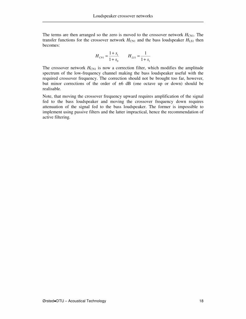
Figure 27 - Amplitude response for the symmetrical third-order three-way crossover
network with a1 = a2 = 2.5 (left) and a1 = a2 = 4 (right).
The conclusion is, that the design would do better without the midrange channel, and this is exactly the following crossover network to be analysed. This is at the end of the ideal filters with H = 1, since higher order filters includes too many terms; they are cumbersome to implement, especially with passive filters.
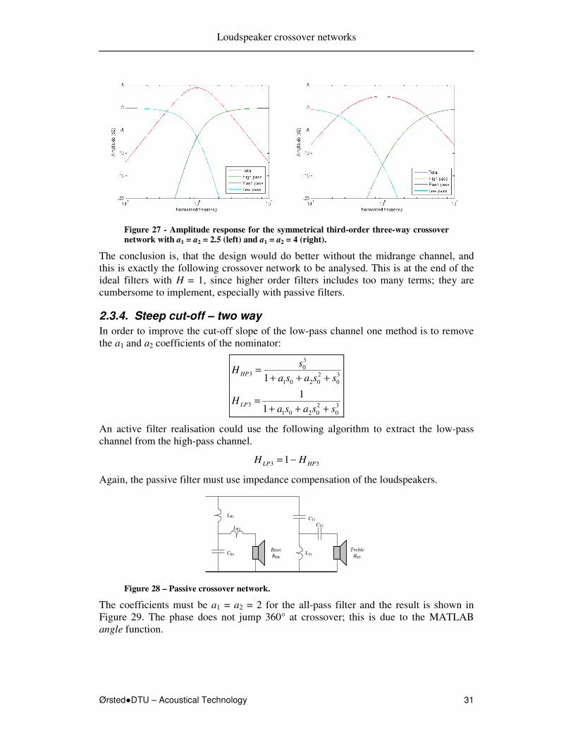
2.3.4. Steep cut-off – two way
In order to improve the cut-off slope of the low-pass channel one method is to remove the a1 and a2 coefficients of the nominator:
3
0
2
0201
3
3
0
2
0201
3
03
1
1
1
ssasaH
ssasa
sH
LP
HP
+++=
+++=
An active filter realisation could use the following algorithm to extract the low-pass channel from the high-pass channel.
33 1 HPLP HH −=
Again, the passive filter must use impedance compensation of the loudspeakers.
Bass
REB
LB1 CT1
Treble
RET LT1 CB1
LB2 CT2
Figure 28 – Passive crossover network.
The coefficients must be a1 = a2 = 2 for the all-pass filter and the result is shown in Figure 29. The phase does not jump 360° at crossover; this is due to the MATLAB angle function.

Loudspeaker crossover networks
ØrstedDTU – Acoustical Technology 32
Figure 29 - Amplitude and phase response with a1 = a2 = 2.
The introduction of a phase different from zero introduces a group delay shown in Figure 30. Note that the group delay unit is calculated for a normalised filter corresponding to a cut-off frequency of 1 Hz. With a cut-off frequency of 1000 Hz the group delay scaling will be in milliseconds and not seconds.
Figure 30 – Group delay with a1 = a2 = 2.
The filter includes two coefficients and its sensitivity to variations was analysed by scaling the coefficients by ±10 % with the result shown in Figure 31.

Loudspeaker crossover networks
ØrstedDTU – Acoustical Technology 33
Figure 31 - Amplitude response for 10 % change of coefficients: a1 = 1.8, a2 = 2.2 (left)
and a1 = 2.2, a2 = 1.8 (right).
The filter accept inversion of the treble loudspeaker.
Figure 32 - Amplitude and phase response with a1 = a2 = 2 and inverted treble.
The group delay is reduced in amplitude and becomes monotonically as result of the inversion, so although one may argument against the inversion, there could be an audible improvement by doing so.
Figure 33 – Group delay with a1 = a2 = 2 and inverted treble loudspeaker.

Loudspeaker crossover networks
ØrstedDTU – Acoustical Technology 34
2.4. Fourth order
Crossover networks of fourth-order are popular due to the steep cut-off slopes, which reduces the loudspeaker requirement to less than 2 octaves beyond the crossover frequency. However, a passive implementation is practical only for the all-pass filter, since component count would be too large with the three-way system.
A fourth-order transfer function is defined from HN with N = 4:
4
0
3
03
2
0201
4
0
3
03
2
02014
1
1
ssasasa
ssasasaH
++++++++
=
2.4.1. Symmetrical – three way
A symmetrical three-way crossover network can be build using the middle term for the midrange loudspeaker. Coefficient a2 must be removed from the nominator.
4
0
3
03
2
0201
014
4
0
3
03
2
0201
2
024
4
0
3
03
2
0201
4
0
3
034
1
1
1
1
ssasasa
saH
ssasasa
saH
ssasasa
ssaH
LP
BP
HP
+++++
=
++++=
+++++
=
An active implementation could use:
444 1 HPLPBP HHH −−=
The low-pass and high-pass channels includes two terms each so they cannot be implemented using standard low-pass and high-pass filters but the circuitry is not too complex to be implemented using active filters. When build, the midrange channel is derived by subtracting the channels from the input signal.
Assume that the coefficients are a1 = 2, a2 = 3 and a3 = 2, to simplify the analysis. The following amplitudes and phases can then be found at the crossover frequency (s0 = i):
°−∠=−+
=+−−+
+=
°∠=−−
=+−−+
−=
°∠=−−
=+−−+
+−=
2432.21
21
12321
21
00.31
3
12321
3
2432.21
21
12321
12
3
3
3
i
ii
iH
iiH
i
ii
iH
LP
BP
HP
So, the low-pass and high-pass channels are 486° out of phase (corresponds to 126°) and adds with some loss and the midrange channel adds the required signal. The channels are all at fairly high levels around crossover so this is a design, which is based upon subtraction of large figures – it should be avoided.

Loudspeaker crossover networks
ØrstedDTU – Acoustical Technology 35
Figure 34 – Amplitude and phase with a1 = 2, a2 = 3, a3 = 2.
2.4.2. Steep cut-off – two way
The terms with a1, a2 and a3 are removed from the nominator resulting in a two-way crossover with maximum cut-off slope within both channels. The filter does not satisfy the requirement of unity transfer function.
4
0
3
03
2
0201
4
4
0
3
03
2
0201
4
04
1
1
1
ssasasaH
ssasasa
sH
LP
HP
++++=
++++=
Determination of the coefficients assume modelling by a combination of two second-order Butterworth filters in cascade (the Linkwitz-Riley method). The nominator polynomial is not important for this evaluation, only the denominator is considered.
( ) 4
0
3
0
2
0
2
0
21
2
00
2
2
00
1224
2221
2,11
scssccs
NN
cwherescs
N
scs
NHHH LPLPLP
+++++=
=++
×++
=×=
By comparison, the coefficients are found to:
83.22
00.42
83.22
3
2
2
1
===+=
==
ca
ca
ca
A passive implementation is at the limit of what can (or should) be done but the network is straight forward from a theoretical point of view. It is a requirement that the loudspeakers are impedance compensated.

Loudspeaker crossover networks
ØrstedDTU – Acoustical Technology 36
Bass
REB
LB1 CT1
Treble
RET LT1 CB1
LB2 CT2
CB2 LT2
Figure 35 – Passive crossover network.
The result is shown in Figure 36. The phase difference between the channels are 360° at crossover so the signals are added without loss.
Figure 36 – Amplitude and phase response with a1 = a3 = 2.83, a2 = 4.00.
Figure 37 – Group delay with a1 = a3 = 2.83, a2 = 4.00.

Loudspeaker crossover networks
ØrstedDTU – Acoustical Technology 37
2.5. Passive network
A passive network is best suited for low order crossover networks and can be build as shown in Figure 38, where Z1, Z2, etc. are impedances, which may consist of resistors, inductors and capacitors or even combinations hereof. The number of branches is defined by the filter order; a first order crossover network would consist of Z1 only.
RE
Z3
Z2
Z1
Figure 38 – Conventional ladder-network for a passive crossover. The impedances can
be any of resistor, inductor or capacitor.
The transfer function of the filter can be derived from inspection of the circuitry. The below collection of crossover network transfer functions is limited to third order since higher order networks become more involved and are of little practical use. Higher order filters should preferably be build using active circuitry.
2.5.1. First order
This consists only of Z1 so Z2 not used and Z3 is a short circuit. The filter is a voltage divider between the series element Z1 and the loudspeaker, represented by the DC voice coil resistance RE. The transfer function for the first order network is:
E
E
RZ
RH
+=
1
1
To introduce real components, the impedance must be substituted by an inductor or a capacitor. The impedance of the inductor and capacitor is defined as:
sCZ
sLZ
C
L
1=
=
Using an inductor for Z1 the result is a low-pass filter:
L
Rwhere
s
R
sLRsL
RH E
E
E
ELP =
+=
+=
+= 0
0
1 ,1
1
1
1 ω
Using a capacitor for Z1 the result is a high-pass filter:
EE
E
E
EHP
CRwhere
s
s
sCR
sCR
RsC
RH
1,
111 0
0
01 =
+=
+=
+= ω

Loudspeaker crossover networks
ØrstedDTU – Acoustical Technology 38
2.5.2. Second order
The crossover network includes Z2, which is shunted across the loudspeaker (since Z3 is a short circuit), so the transfer function can be derived from H1 by substituting RE by a parallel combination of Z2 and RE:
2121
2
2
21
2
2
2
ZZR
ZZ
Z
RZ
RZZ
RZ
RZ
H
EE
E
E
E
++=
++
+=
Using an inductor for Z1 and a capacitor for Z2 the result is a low-pass filter:
sCsL
sCRsL
sCH
E
LP 11
1
2
++=
After reduction:
C
L
RQa
CLwhere
ssaH
E
LP
111,
1
1102
001
2 ===++
= ω
Using a capacitor for Z1 and an inductor for Z2 the result is a high-pass filter:
EE
EHP
sLRRsC
sLsC
sLRH
++=
112
After reduction:
C
L
RQa
CLwhere
ssa
sH
E
HP
111,
1102
001
2
02 ===
++= ω
2.5.3. Third order
Derivation starts from the loudspeaker where Z3 forms a voltage divider with RE. The two first components also forms a voltage divider between Z1 and Z2, where Z2 is in parallel with Z3 + RE.
( )
( )E
E
E
E
E
E
RZ
R
RZZ
RZZZ
RZZ
RZZ
H+
+++
+
+++
=3
32
321
32
32
3
After reduction::
EE
E
RZZZRZZZZZ
RZH
23213121
23 ++++
=

Loudspeaker crossover networks
ØrstedDTU – Acoustical Technology 39
Using an inductor for Z1 and Z3 and a capacitor for Z2 the result is a low-pass filter:
( ) 1
1
111
1
22
323
++++=
++++=
EEE
EE
E
LP
R
sLCLs
R
CLs
R
LsR
sCsL
sCsLRsL
sCsL
RsCH
After reduction:
2
322
31
320
3
0
2
0201
3
1
1
1
===
+++=
CL
RCLa
C
LR
Ra
CL
R
ssasaH
EE
E
E
LP
ω
Using a capacitor for Z1 and Z3 and an inductor for Z2 the result is a high-pass filter:
CLsR
Ls
sCRR
Ls
CLs
sLRsC
sLRsCsC
sLsC
sLRH
EEEEE
E
2
2
23
111111 ++++
=+++
+=
After reduction:
2
322
31
320
3
0
2
0201
3
03
1
1
===
+++=
CL
RCLa
C
LR
Ra
CL
R
ssasa
sH
EE
E
E
LP
ω
2.5.4. Fourth order
Filter realisation will use the ladder-network shown in Figure 39, which is a general filter using impedances.
Z1
EG Z2
Z3
Z4 RL EL
E2
Figure 39 – Generic ladder-filter for realisation of the crossover networks. The
impedance Z represents any combination of capacitors (Z = 1/sC), inductors (Z = sL)
or resistors (Z = R). The load resistor RL represents the loudspeaker.
The voltages at the nodes are, according to Kirchhoff’s law, which states that the sum of currents to a node must equal zero (with positive direction defined away from the node):
0
0
43
2
3
2
2
2
1
2
=++−
=−
++−
L
LLL
LG
R
E
Z
E
Z
EE
Z
EE
Z
E
Z
EE

Loudspeaker crossover networks
ØrstedDTU – Acoustical Technology 40
The terms are rearranged:
L
L
L
L
LG
ER
Z
Z
ZE
Z
EE
RZZ
Z
E
Z
EE
ZZZ
++=⇒=−
++
=−−
++
3
4
32
3
2
43
31
2
321
10111
0111
Elimination of E2 results in:
13
3
4
3
321
1111
Z
E
Z
EE
R
Z
Z
Z
ZZZ
GLL
L
=−
++
++
And:
13
3
4
3
321
11
111
Z
EE
ZR
Z
Z
Z
ZZZ
GL
L
=
−
++
++
And:
GL
L
EEZ
Z
R
Z
Z
Z
Z
Z
Z
Z=
−
++
++
3
13
4
3
3
1
2
1 11
The transfer function becomes:
3
13
4
3
3
1
2
1 11
1
Z
Z
R
Z
Z
Z
Z
Z
Z
ZE
EH
L
G
L
−
++
++
==
2.5.5. Loudspeaker impedance
All passive crossover networks are sensitive to the load impedance and they are most often designed for constant and resistive loading; but the impedance of a loudspeaker is neither constant nor resistive as can be seen from Figure 40. The impedance is real only at very low frequencies and changes from capacitive to inductive within the pass band.

Loudspeaker crossover networks
ØrstedDTU – Acoustical Technology 41
Figure 40 – Electrical impedance of loudspeaker with resonance frequency normalised
to unity, with voice coil cut-off frequency set to 30 times the resonance frequency and
with mechanical quality factor QM = 5.
A passive crossover network will not operate as intended if loaded by this impedance so the presumptions of the filter will be validated and the result can be rather dramatic.
R1
L1
C1
R2
C2
RE
Figure 41 – Compensation networks for loudspeaker impedance correction.
Consider a treble loudspeaker with 1 kHz resonance frequency, which is to be activated above 4 kHz by a series capacitor. The required attenuation at the crossover frequency is (1 kHz)/(4 kHz) = 0.25, so the capacitor must have an impedance of 4 times the nominal impedance at this frequency. But the impedance of the loudspeaker may have increased to 4 times the nominal value, thus compensating for the rise in impedance; the effective crossover frequency becomes the resonance frequency of the loudspeaker.
It is possible to compensate, at least partially, for the variation in loudspeaker impedance, using networks shown Figure 41, thus introducing additional components increasing complexity and cost.
The equations for the correction networks are shown below [2]. The required parameters are the electrical and mechanical quality factors (QEC and QMC) and the resonance frequency (fC) of the loudspeaker in the closed cabinet, the DC resistance of the voice coil (RE), and the inductance of the voice coil (LE).
ECEC
C
ECE
E
MC
EC
QRfC
f
QRL
RQ
QR
π
π
2
1
2
1
1
1
1
=
=
+=
22
1
2 E
E
E
R
LC
RR
π=
=

Loudspeaker crossover networks
ØrstedDTU – Acoustical Technology 42
Midrange loudspeaker: QEC = 0.4, QMC = 3, fS = 80 Hz, RE = 6 Ω.and LE = 0.1 mH.
Compensation of the resonance frequency: R1 = 6.8 Ω, L1 = 4.8 mH and C1 = 800 µF.
Compensation of the voice coil inductance: 6 Ω and 0.44 µF.
It is not required compensating for the resonance frequency of a bass loudspeaker, since this is within the pass band of the crossover network and similar arguments are valid for the voice coil inductance of the treble loudspeaker. A midrange loudspeaker may require compensation of both parameters.
An active crossover network solves the problem of interaction between the crossover network and the loudspeaker. It offers better control of filter parameters, since inductors can be avoided, and it is insensitive to the temperature dependency of the voice coil DC impedance. Problems, which must be addressed by the designer of a passive crossover network, in addition to the more obvious problems of selecting the crossover frequencies, deciding a network topology and how to construct the loudspeaker system from available components.
2.6. Active network
Active networks are build from filter blocks, such as the two blocks shown in Figure 42. Amplifiers are used as buffers avoiding interaction between the filter sections. It should be mentioned that the layout possibilities are large and the below examples represents but a few of the possible implementations.
First-order filter block Second-order filter block
RE
Z5
Z4
Z3
Power amplifier and
loudspeaker
Z6
Buffer Buffer
Z1
Z2 E1 E2 E3
A
B
Figure 42 – Active filter consisting of a first-order filter block and a second-order
filter block. The amplifiers isolates the sections thus simplifying the design.
Active filters are designed from resistors, capacitors and amplifier circuits. The inductor is not required and has been omitted since it is difficult to build good inductors; they are plagued by their series resistance and parallel capacitance and the component is prone to pick-up of hum from magnetic fields. The resistor and capacitor are almost ideal components with few parasitic components. The missing inertia, offered by the inductor in the passive crossover networks, and required by circuits with complex poles, is supplied by the amplifier.
In this example is the amplifier arranged as a voltage-follower, which means that it monitors the voltage at the input without loading the circuitry and outputs the voltage. The gain factor (amplification factor) is unity.

Loudspeaker crossover networks
ØrstedDTU – Acoustical Technology 43
2.6.1. First order
The filter is actually a passive filter since one of the components are a resistor and the other a capacitor. The network is energised from node E1 with output at node E2.
CR
ssCRH
s
s
sCR
sCRH
ZZ
Z
E
EH
LP
sCZRZ
HP
RZsCZ
1
1
1
1
1
11
0
0
1/1
0
01/1
21
2
1
21
2
1
2
1
=
+=
+= →
+=
+= →
+==
==
==
ω
2.6.2. Second order
The transfer function is best derived from the Kirchhoff law of nodes, which states that the sum of current into a node must equal zero. There are two internal nodes, A and B, but node B is identical to the output node E3 due to the buffer. The network is energised from node E2 with output at node E3. The equations are:
0
0
4
3
5
3
5
3
4
3
3
2
=+−
=−
+−
+−
Z
E
Z
EE
Z
EE
Z
EE
Z
EE
A
AAA
After reduction:
64
53
6
532
32
1
1
ZZ
ZZ
Z
ZZE
EH
++
+==
Using resistors for Z4 and Z6 and capacitors for Z3 and Z5 results in a high-pass filter:
1
2
21
21
2121
02
00
2
02
11,
1 R
R
CC
CCQ
aRRCCwhere
sas
sH HP +
===++
= ω
Using resistors for Z3 and Z5 and capacitors for Z4 and Z6 results in a low-pass filter:
2
1
21
21
2121
02
00
2
11,
1
1
C
C
RR
RRQ
aRRCCwhere
sasH LP +
===++
= ω
2.6.3. Higher orders
Filters of higher order can be build from first and second order filter blocks by cascading the filters. A seventh order two-way crossover network will be used as an example:
2
003
2
002
2
0010
7
2
003
2
0
2
002
2
0
2
001
2
0
0
07
1
1
1
1
1
1
1
1
1111
ssassassasH
ssa
s
ssa
s
ssa
s
s
sH
LP
HP
++×
++×
++×
+=
++×
++×
++×
+=

Loudspeaker crossover networks
ØrstedDTU – Acoustical Technology 44
All blocks share the same cut-off frequency, given by ω0, with the Butterworth design but the coefficient a1, a2 and a3, are different. The coefficients determine the roots of the denominator polynomial. The root of the first order polynomial is s0 = –1, and the roots of the second order polynomials are determined from:
01 2
00 =++ sas
The roots are:
2
4
2
4 22 aiaaai
−±−=
−±−=± βα
It follows that both the real part and imaginary parts of the roots (α and β respectively) are defined by the coefficient a. Hence, the value is given by:
α2−=a
For the seventh order Butterworth polynomial are the roots defined as shown below in Table 2, which also shows the calculated values of the coefficients as well as the quality factors Q = 1/a:
Table 2 – Coefficients for a seventh order crossover network. The real value of the
root determines the coefficient and thus the quality factor.
Section Roots Coefficient a Quality factor Q
1 (-1) - -
2 (-0.2225 ±i0.9749) 0.445 2.247
3 (-0.6235 ±i0.7818) 1.247 0.802
4 (-0.9010 ±i0.4339) 1.802 0.555
The coefficient could as well be determined from the imaginary root value, which gives the same result. Take for instance the last root. With a = 1.802 is imaginary value:
( )4338.0
2
802.14
2
422
±=−±
=−±
=aβ
This is indeed the specified value.
2.6.4. Special
Several of the crossover networks used an algorithm such as the following for derivation of the low-pass channel from a steep high-pass channel.
33 1 HPLP HH −=
This can relative easily be implemented as shown below where the input signal is high-pass filtered and routed through a power amplifier to the treble loudspeaker as well as to a subtraction circuitry for construction of the low-pass channel.
The high-pass filter is realised as a conventional third-order filter and a subtraction network (an operational amplifier) is used to generate the low-pass channel.

Loudspeaker crossover networks
ØrstedDTU – Acoustical Technology 45
Power amplifier
High-pass
filter
Bass
Power amplifier
Σ Treble
-
+
Input
3
0
2
0201
3
0
1 ssasa
s
+++
3
0
2
0201
2
0201
3
0
2
0201
3
0
1
1
11
ssasa
sasa
ssasa
s
+++++
=+++
−
1
Figure 43 – Active crossover network.

Loudspeaker crossover networks
ØrstedDTU – Acoustical Technology 46
3. Models A loudspeaker is not just a linear transducer that outputs sound as a true replica of the input signal; the loudspeaker, the baffle and the listening room introduces limitations, severely affecting the signal quality. The loudspeaker bandwidth is limited and it is not small compared to wavelength at high frequencies, which affects the radiation angle concentrating the sound at the front of the loudspeaker. The front baffle introduces an impedance discontinuity at the edges, which cause reflections known as diffraction, that interferes with the direct signal and results in the well-known 6 dB loss of bass as well as ripples at higher frequencies. Listening off-axis introduces time difference for signals from the different loudspeakers, which create ripples around the crossover frequency, and reflections from large surfaces further affects the low frequency reproduction.
The model derived in this section is a transfer function for analytical studies using MATLAB. The models apply solely to the electro-dynamic loudspeaker using a moving-coil for the energy transfer; so electrostatic, piezoelectric and ribbon-type loudspeakers are not referenced.
At first, a model for the loudspeaker is introduced and this is followed by models for the surrounding; i.e. diffraction due to the baffle, the listening angle due to the distance between the loudspeakers and the reflections from the boundaries of the listening room. A model is also introduced for the calculation of group delay based upon the resultant transfer function.
3.1. Electro-acoustical model
The transfer function model for the loudspeaker consists of several terms each describing a specific part of the loudspeaker. The result is the sound pressure p at distance r with an number of parameters describing the loudspeaker.
( ) GREF
DVC EKikrr
rHHp ×
×−××= exp
The excitation voltage EG from the power amplifier is converted to a sound pressure by the constant K, which assembles the electrical, mechanical and acoustical parameters and represents the sound pressure within the middle of the pass-band at a reference distance rREF, but it does not include parameters such as frequency and angle. The useful frequency range is specified by HVC for the voice coil high-frequency cut-off and by HD for the low frequency cut-off. The inverse-distance law is specified by rREF/r, and the exponential function. The model can easily be enhanced by introducing more functions dealing with specific areas.
Derivation starts by analysing the mechanical construction of the loudspeaker and the following analysis will be based upon the introduction presented by Leach and with reference to Beranek. The loudspeaker model applies to bass, midrange and treble units and will be limited to units with the rear side radiating into a closed cavity thus realising a single model common to all the loudspeaker units.

Loudspeaker crossover networks
ØrstedDTU – Acoustical Technology 47
Electrical
system
Voltage
EG, EM
Current
IC
Generator voltage
EG
Mechanical
system
Force
FM, FA
Velocity
UD
Acoustical
system
Pressure
pD
Volume velocity
SDUD
Front ZAF
Sound pressure
pD
Rear ZAR
Voice coil current
IC
Volume velocity
SDUD
Radiation resistance
Figure 44 – The model is based upon the model of a loudspeaker and operates with
three different system analogies: electrical, mechanical and acoustical.
The initial part of the analysis concentrates on deriving a model for the diaphragm velocity as a function of generator voltage, which introduces the loudspeaker frequency dependency. The diaphragm velocity is converted into sound pressure, which introduces the inverse-distance law. The remaining analysis deals with the consequence of diaphragm diameter, monitoring angle and the baffle size thus introducing directivity and diffraction. The consequence of reflections from the listening room will also be considered.
It is common to divide the loudspeaker unit into three different system analogies as shown in Figure 44. The electrical system is responsible for the voice coil current, the mechanical system translates this into diaphragm velocity and the acoustical system accounts for sound pressure, air loading and the effect of the closed cabinet.
3.1.1. The loudspeaker unit
A layout of the electro-dynamic loudspeaker is sketched in Figure 45, which also displays the main difference between the bass/midrange and treble units. The diaphragm of the treble unit is reduced to a dome to cut the mass and the size of the loudspeaker thus improving reproduction of the high-frequency range.
The diaphragm is the moving surface of the loudspeaker which radiates sound. The preferred material is paper, due to its low weight and high internal damping, although plastic and metal are also used. The diaphragm is cone or dome shaped to improve rigidity although loudspeakers with flat diaphragm exists. A suspension system is used to keep the diaphragm at the correct position with the voice coil within the magnet gap and restrict the diaphragm movement to the axial direction only.
The effective diameter of the diaphragm (D) includes some of the outer suspension, which is moving as well, so the effective cross-sectional area becomes:
22
4DaSD
ππ ==
The area is 300 cm2 for an 8 inch loudspeaker and 5 cm2 for 1 inch diameter.
For treble loudspeakers is the diaphragm a dome and the equation is gives a rough estimate when the dome is approximately one-quarter of a sphere.

Loudspeaker crossover networks
ØrstedDTU – Acoustical Technology 48
Suspension
Diaphragm (cone)
Magnet
D
Air gap
Diaphragm (dome)
Suspension
D
Dust cover
Mounting base
Mounting base
FRONT side of the diaphragm
REAR side of the diaphragm
Maximum linear
displacement
Voice coil
a
Figure 45 – Model of bass and midrange units (left) and treble units (right). The main
difference between units is the mass of the moving system and the effective cross-
sectional area of the diaphragm.
The loudspeaker will be assumed sealed to interrupt the radiation from the rear of the diaphragm thus reducing the complexity of the model. The intention is that the same model should apply to all loudspeaker units with adjustment of parameter values. Treble units are almost always sealed and midrange units most often include a can at the rear side. The bass loudspeakers are never sealed and must be placed within a closed cabinet.
As will be shown later in this section, the loudspeaker is a transducer where the transfer function is a band-pass filter with a frequency range determined by the moving system and the voice coil. The sound pressure is downward limited by the resonance frequency below which any closed-box loudspeaker systems will drop off at 12 dB/octave and the sound pressure is upward limited by the electrical low-pass filter of the voice coil resistance and inductance above which the response drops off by –6 dB/octave.
The model assumes that the loudspeaker diaphragm is vibrating as a rigid piston. This is
true for low frequencies where the diaphragm circumference 2πa is short compared to
wavelength λ. This is most often expressed as ka < 1, where frequency is represented by the angular wave number k:
a
cf
c
f
ckka
πλππω
2
221 <⇒===∧<
A loudspeaker with diameter a= 0.05 m becomes directive above approximately 1.1 kHz.
A loudspeaker can be assumed equivalent to a monopole sound source at low frequencies (ka < 1) where radiation is equally well in all directions. The loudspeaker becomes directive at high frequencies (ka > 1) where the output becomes concentrated on the loudspeaker axis and the off-axis output is limited. At higher frequencies (ka > 3) may the diaphragm break up and vibrate in sections with different phases, which affects both amplitude and directivity.

Loudspeaker crossover networks
ØrstedDTU – Acoustical Technology 49
3.1.2. Electrical circuit
Electrical variables are the voltage difference E and current I and the electrical impedance is defined by:
Ω==A
Vunit
I
EZE :
Input to the loudspeaker is an applied voltage EG from an external voltage generator with an internal series impedance ZG, see Figure 46. The resulting voice coil current IC generates a voltage drop across the generator impedance of:
CG IZE =1
The voice coil current flows through the voice coil resistance RE and inductance LE. The voice coil is shown in parallel with a resistor RL to model the effect of eddy current losses in the magnetic circuit. The voltage across the voice coil is given by:
C
LE
LEE I
RsL
RsLRE ×
++=2
When the voice coil and diaphragm is moving with velocity UD, a voltage is induced into the voice coil wire:
DM UBLE ×=
The product of the magnet flux density B and the effective length of the voice coil wire L is the force factor, which is specified in the loudspeaker data sheet. We now know the individual terms of the electrical system.
Generator impedance
ZG
Generator voltage
EG
Voice coil resistance
RE
Voice coil inductance
LE
Voice coil voltage
EM
Voice coil current
IC
E2 E1
External Internal
Eddy current
RL
Figure 46 – Electrical model of loudspeaker input with the generator EG representing
the power amplifier and with the voice coil DC resistance RE and the inductance LE.
The feedback from the moving system is represented by the second voltage source EM.
The relation between generator voltage EG, voice coil current IC and diaphragm velocity UD can now be derived by Kirchhoff’s law, which states that the sum of all voltages within a closed mask must equal zero. It follows that:
MC
LE
LEEGG EI
RsL
RsLRZE +×
+++=
The generator impedance is often ignored since the output impedance approximates zero in most situations. This assumption will be used to simplify the expressions, but the ZG can be re-introduced at any time by substituting RE with RE + ZG.

Loudspeaker crossover networks
ØrstedDTU – Acoustical Technology 50
fC fL
-6 dB/octave
Hence, the voice coil current becomes:
E
MG
L
E
E
E
L
E
LE
LEE
MGC
R
EE
R
R
R
sL
R
sL
RsLR
RsLR
EEI
−
++
+=
++
−=
11
1
The equation includes a filter with a cut-off frequency (pole frequency fC) due to the voice coil series resistance RE and inductance LE and a correction due to the eddy current losses represented by RL (null frequency fL). The frequencies are:
E
LLL
E
E
E
L
EE
CC
L
Rf
L
R
L
R
RR
f
ππω
πππω
22
22
1
2
==
≈
+
==
For RE = 5 Ω and LE = 1 mH is fC = 800 Hz (ignoring RL) so the higher frequencies are
attenuated by –6 dB/octave. For RL = 100 Ω is fL = 16 kHz above which the attenuation ceases.
The voice coil current is represented by:
E
MGVCC
R
EEHI
−=
The transfer function HVC due to the voice coil is defined by:
C
L
C
L
C
LVC
s
s
s
s
s
s
H++
=++
=+
+=
1
1
1
1
ωω
ω
ω
For low frequencies is HVC = 1, which indicates that the voice coil current IC is proportional to the difference between the excitation voltage EG and the velocity-induced voltage EM and that the correlation constant is the DC resistance of the voice coil RE. For high frequencies are the voice coil current reduced since the impedance of the inductance LE is becoming the dominating term.
3.1.3. Mechanical circuit
Mechanical variables are force F and velocity U, which are analogue to voltage and current in electrical systems although the electrical current flows through series-connected components, whereas the velocity in mechanical systems is common to parallel-connected components. The mechanical impedance is defined by:
s
kg
m
Nsunit
U
FZM == :

Loudspeaker crossover networks
ØrstedDTU – Acoustical Technology 51
The motor of the loudspeaker is the voice coil, which is located within the strong magnetic flux of the air gap. The electrical current IC within the voice coil results in a mechanical force working on the voice coil:
CM IBLF ×=
A typical value of BL is 10 N/A so a voice coil current of one ampere results in a force on the voice coil of 10 N, which is approximating the weight of a 1 kg plumb.
A pressure difference between the front and rear side of the diaphragm results in a force working on the diaphragm, which is the pressure difference multiplied by the area:
( ) DDRFDA pSppSF =−=
For an 8 inch loudspeaker with a diaphragm area SD = 0.032 m2, and a pressure difference of pD = 1 Pa, corresponding to 94 dB sound pressure level, the force from the acoustical system becomes fA = 0.032 N, which is small compared to the mechanical forces involved so the reaction from the acoustic system can be ignored in some applications.
The resultant force working upon the mechanical system becomes:
AMR FFF −=
The direction of the forces has been selected so FM > 0 drives the diaphragm forward while FA > 0 drives it backward. This is an arbitrary choice, but it models the actual behaviour of the loudspeaker where the mechanical force is opposed by the force from the acoustical system.
Moving mass
MMD
Suspension compliance
CMS
Suspension losses
RMS
Electrical force
fM
Diaphragm velocity
uD
Acoustical force
fA
Figure 47 – Mechanical model of loudspeaker moving system (mobility analogy). The
mass of voice coil and diaphragm are assembled into MMD, the suspension system is
represented by the spring compliance CMS and the friction losses by RMS.
Typical values for an 8 inch loudspeaker are: MMD = 80 10-3 kg, CMS = 500 10-6 m/N and RMS = 3 kg/s.
The mechanical system consists of the mass MMD of voice coil and diaphragm, and of the compliance CMS and friction losses RMS of the suspension system. The diaphragm velocity UD is described as the solution to the following differential equation:
AMD
MS
DMSD
MD FFdtuC
uRdt
duM −=++ ∫
1
The first term is due to the law of motion, FM = MMDaD, where aD = duD/dt is the acceleration of the diaphragm. The second term is the relation between force and friction losses, FR = RMSuD. The third term is due to compliance, FC = xD/CMS, where xD is the diaphragm displacement and is related to velocity by uD = dxD/dt.

Loudspeaker crossover networks
ØrstedDTU – Acoustical Technology 52
The mechanical system is completely described by the resonance frequency fS and the quality factor QS.
MS
MD
MS
S
MSMD
S
C
M
RQ
CMf
1
2
1
=
=π
In the frequency domain is the equation easy to solve for diaphragm velocity:
AMD
MS
MSMD FFUsC
RsM −=
++
1
This can be written:
MS
MSMDMAMDMsC
RsMZwhereFFUZ1
++=−=
The corresponding circuit model is shown in Figure 48.
Electrical force
FM
Suspencion losses
RMS
Moving mass
MMD
Acoustical force
FA
Compliance suspension
CMS
Diaphragm velocity
UD
Figure 48 – Impedance analogy of the mechanical system. The mass and compliance
cancels at the resonance frequency where the diaphragm velocity is maximum.
The diaphragm velocity is maximum around the resonance frequency where ZM ≈ RMS and is in phase with the excitation. Below the resonance frequency will the diaphragm velocity increase with increasing frequency and the phase approaches +90°, while the diaphragm velocity decreases with frequency above the resonance frequency where the phase approaches –90°, compared to the excitation.
3.1.4. Acoustical circuit
Acoustical variables are the pressure difference p and volume velocity SU, which are analogue to voltage and current in electrical systems. The volume velocity is in this study represented by the diaphragm cross-sectional area S multiplied by the velocity, hence the variable SU. The acoustical impedance is defined by:
23:
sm
kg
m
Nsunit
SU
pZ A ==
Two different load impedances will be analysed below; the loading at the front side of the diaphragm, which is assumed radiating into free space, and the loading at the rear side, which is radiating into a closed cabinet.
The front side of the diaphragm is loaded by air and the impedance is defined in [3] for a circular piston at the end of an infinitely long tube. The impedance consists of a mass term, which dominates for ka < 1, and a frequency-dependent resistive term, which

Loudspeaker crossover networks
ØrstedDTU – Acoustical Technology 53
dominates at higher frequencies and approximates a constant for ka > 2. The resulting impedance is a parallel combination of:
2
00 318.0195.0a
cRand
aM AFAF
ρρ≈≈
Examples are MAF = 2.3 kg/m4 and RAF = 20 103 kg/sm4 for a = 0.1 m (8 inch loudspeaker). The impedances are transformed to the mechanical circuit by multiplication with SD
2. For
SD = πa2 = 30 10-3 m2 the values become: MMF = 2.3 g and RMF = 20 103 kg/s.
The mass term represents a volume of uncompressed air, which is moving with the diaphragm velocity. The resistance term represents the energy lost into the air.
Since the components are in parallel the total impedance becomes:
AF
AFAFAF
AF
AF
AFAF
AFAFAF
M
Rfwhere
s
sM
RsM
RsMZ
ππω
ω22
1
==+
=+
=
The cut-off frequency fAF is 1.4 kHz for the 8 inch loudspeaker.
A fair representation is a mass MAF at low frequencies (LF) and a resistor RAF at high frequencies (HF), which will be represented as follows (ka limits from [3]):
( ) ( ) 55.0 >=<= kaforRZandkaforMZHF
AFAF
LF
AFAF
The rear side of the loudspeaker is loaded by the closed cabinet, which is represented by an acoustical impedance with CAB for the compliance of the confirmed air, MAB for the air load on the rear side of the diaphragm and RAB for the losses within the box. The acoustical loss within the closed box RAB cannot easily be calculated and must be estimated by other means; but luckily, the value is of minor importance, at least for this study, and can safely be ignored. The compliance and mass load can be calculated by the following approximations, which assumes that the box is small and without any damping material.
aMand
c
VC AB
ABAB π
ρρ
0
2
0
65.0≈≈
A box is small when the largest dimension is less than λ/10, which corresponds to the following design requirement where LB represents the largest box dimension:
BL
cf
10>
The equivalent circuit for the loading of the loudspeaker is shown in Figure 49, with the rear of the loudspeaker radiating into a closed box and the front into free space.

Loudspeaker crossover networks
ØrstedDTU – Acoustical Technology 54
Acoustical
losses
RAB
Moving air mass
MAB
Box compliance
CAB
Air load mass
MA1
Volume velocity
SDUD
pD
Sound pressure
difference
Air load resistance
RA1
Figure 49 – Load impedances for the loudspeaker.
Hence, the sound pressure difference between the loudspeaker front and rear side:
( ) ( ) ( ) DDARAFDD
AB
ABAB
HF
AF
LF
AFD USZZUSsC
RsMRsMp +=
++++=
1
Radiation resistance ZAF is a function on loudspeaker mounting. The loudspeaker may be approximated by a monopole sound source at low frequencies but the loudspeaker baffle comes into play at higher frequencies and the model is then approximately a monopole close to an infinite wall, which doubles the sound pressure. The transition between the two models is unfortunately not straightforward.
The model should also include the interaction between two sources operating at the same frequency (i.e. at cross-over) and the reflections from cabinet boundary (diffraction). In order to separate the different models, the loudspeaker model will load the front of the loudspeaker by the radiation impedance of a plane piston in an infinite tube. This models the monopole sound source and the other factors can then be added to the model without a need of changing the basic model.
3.1.5. Diaphragm velocity
The first step is to derive a relation between the diaphragm velocity UD and generator voltage EG and the final step is to determine the sound pressure.
Two expressions are at hand for the voice coil current IC and using them to eliminate the voice coil current introduces EG, UD and the force FM from the voice coil.
( )E
DGVCM
M
E
DGVCC
R
UBLBLEHF
BL
F
R
BLUEHI
2−×=⇒=
−×=
HVC represents the voice coil high-frequency attenuation, which is unity for frequencies below approximately 500 Hz.
Another expression for FM is available introducing the mechanical impedance ZM and the force from the acoustical system FA, which again introduces the acoustical impedances ZAF and ZAR for the loading on the loudspeaker front and rear sides.
( ) DDARAFDMMADMM USZZUZFFUZF2++=⇒+=
Elimination of FM results in the following equation for estimation of diaphragm velocity UD versus generator voltage EG.
( ) ( ) DDARAFMD
E
DGVC USZZZU
R
UBLBLEH
2
2
++=−
×

Loudspeaker crossover networks
ØrstedDTU – Acoustical Technology 55
The expression is solved for diaphragm velocity UD as a function of EG:
( ) ( )G
E
VC
DARAFM
E
VC
D ER
BLH
SZZZR
HBLU ×××
+++=
2
2
1
The first term is consists of mechanical impedances with the voice coil HVC transformed to the mechanical system by (BL)2, and the acoustical impedances transformed by SD
2.
The (BL)2HVC/RE term represents the damping from the electrical system. The term is
active around resonance where the denominator consists of (BL)2/RE plus the frequency-independent terms from ZM, ZAF and ZAR (the reactive terms cancel at resonance). The (BL)2/RE term is gradually removed at high frequencies due to HVC, but the denominator is dominated by the mass-term of ZM above resonance, so HVC can be ignored without consequences at higher frequencies. This can be seen from the following inequity, which states the requirement for the mass term to dominate over the (BL)2/RE term:
( ) ( )MDE
MDMD
E MR
BLfMsM
R
BL
πω
2
22
>⇒=<
For BL = 10 N/A, RE = 5 Ω and MMD = 0.050 kg is f >160 Hz. The HVC term is unity for frequencies below approximately 500 Hz, so the correction due to HVC can be ignored.
Using this simplification and introducing the definitions for the mechanical impedance ZM and the radiation resistance ZAF and ZAR the equation becomes.
( ) ( ) ( ) 2
211
D
AB
ABAB
HF
AF
LF
AF
MS
MSMD
E
G
E
VC
D
SsC
RsMRsMsC
RsMR
BL
ER
BLH
U
++++++++
××=
As stated before, the acoustical impedance for the front of the diaphragm consists of two contributions, the mass MAF, which is effective at low frequency (ka < 0.5), and the resistance RAF, which is effective at high frequency (ka > 5). Note that the two terms are not active at the same time, hence the notation with super fixes LF and HF.
As will be seen in the following, the resistance term RAF is of no importance for the definition of the resonance frequency, since the resonance frequency this is a low-frequency parameter, and it will be completely masked by the mass of the moving system at high frequencies, hence RAF will never contribute to the transfer function and will be ignored.
The above simplifications do not limit the useful frequency range of the model; we are simply deleting terms, which will never contribute to the result. The model is thus valid from the extreme low-frequency range and up to the limit where the loudspeaker diaphragm breaks up, i.e. about around ka = 3.

Loudspeaker crossover networks
ØrstedDTU – Acoustical Technology 56
The following definitions will be introduced to ease the analysis: MMS, which is the moving mass of the total system, RMT, which is the mechanical resistance of the total and CMT, which is the mechanical compliance of the total system:
( )( )
2
2
2
2
2
2
2
11
D
ABMS
D
ABMS
ABMSD
ABMSMT
AB
D
MSMT
DABMS
E
MT
DABAFMDMS
S
CC
S
CC
CCS
CCC
sC
S
sCsC
SRRR
BLR
SMMMM
+=
+=⇒+=
++=
++=
Hence, the following equation for the diaphragm velocity:
G
E
VC
MT
MTMS
D ER
BLH
sCRsM
U ×××++
=1
1
The equation is multiplied and divided by RMT and the nominator and denominator are multiplied by sCMT thus resulting in a second-order denominator polynomial in s.
G
EMT
VC
MTMSMTMS
MTMTD E
RR
BLH
CsRCMs
CsRU ×××
++=
12
The resonance frequency fS is identified as the frequency where s2MMSCMT + 1 = 0:
MTMS
SS
CMf
ππω
2
1
2==
The second-order term is normalised to (s/ωS)2 and the first-order term sRMSCMT is
normalised as follows:
MS
MTMT
SMTMS
MTMT
S
MTMTS
S
MTMTM
CR
s
CM
CRsCR
sCsR
ωωω
ω===
The constant factor to s/ωS is dimension-less and is identified as the total quality factor
for the loudspeaker in a closed cabinet:
MT
MS
MT
TSC
M
RQ
1=
The total quality factor is sensitive to both the electrical, mechanical and acoustical systems but damping from the electrical system is the dominating factor.
QTS = 0.50 corresponds to a critically damped system, which should theoretically reproduce transients without oscillations. The level is 6 dB down at the resonance frequency, which can be compensated electronically by a bass boost from the amplifier.
QTS = 0.71 corresponds to a Butterworth filter with –3 dB at the resonance frequency and some oscillations with transient input. It is often called the maximally flat alignment.

Loudspeaker crossover networks
ØrstedDTU – Acoustical Technology 57
QTS = 1.00 corresponds to a 1 dB Chebychev filter with 0 dB at the resonance frequency, a peaking of 1 dB above the resonance frequency and oscillations with transients.
It is common to divide the quality factor into electrical and mechanical quality factors by the use of the definition for RMT and ignoring the acoustical resistance, which is small compared to the two others.
( ) MSES
MSESTS
MS
MS
MS
MS
MS
MSEES
QQQ
C
M
RQ
C
M
BL
RQ
+===
12
The quality factor is proportional to RE. This reflects the recommendation, found in many loudspeaker books and magazines, that a bass loudspeaker should not be driven from a high-impedance source. This would otherwise increase the effective value of RE (which is in series with ZG) and result in a booming bass.
The transfer function for diaphragm velocity UD as a function of generator voltage EG can then be expressed as follows:
G
EMT
VC
STSS
STSD E
RR
BLH
s
Q
s
s
QU ×××
++
=
11
1
2
ωω
ω
The expression for the diaphragm velocity is a band-pass filter centred at the resonance frequency and with symmetrical skirts. The diaphragm velocity is maximum at the resonance frequency and less for all other frequencies.
3.1.6. Sound pressure
Derivation of the sound pressure from the loudspeaker uses the equation for the sound pressure at distance r from a monopole sound source in free space. The sound pressure is specified with a given volume velocity SDUD and is [3]:
( ) ( ) DDUSikrr
irp −= exp
40
πωρ
The exponential is a complex unit vector which defines the phase due to the delay of the sound waves travelling the distance r from the source to the monitoring point where k is
the angular wave number (k = ω/c).
The sound pressure becomes:
( ) ( ) G
EMT
VC
STSS
STSD E
RR
BLH
s
Q
s
s
QSikr
r
irp ×××
++
×−=
11
1
exp4 2
0
ωω
ωπ
ωρ

Loudspeaker crossover networks
ØrstedDTU – Acoustical Technology 58
Which can be rearranged into five terms: two transfer functions, one angular transfer function, a constant expression and the excitation voltage:
( ) ( ) G
EMTTS
DS
STSS
SVC E
RRrQ
BLSikr
s
Q
s
si
Hrp ××−×
++
×=
πωρ
ωω
ωω
4exp
11
02
2
The resonance frequency has been included into the constant expression in order to simplify the expression.
Using the relation s = iω and introducing a reference distance rREF, the resultant transfer function for the sound pressure p(r) at distance r given by the excitation voltage EG:
( ) ( ) GREF
DVC KEikrr
rHHrp ×−××= exp
The transfer function due to the mechanical system is:
11
2
2
++
=
STSS
S
D
s
Q
s
s
H
ωω
ω
The constant K assembles the scaling factors:
EMTTSREF
DS
RRQr
BLSfK
20ρ
=
Expressing RMT by the definition of the total quality factor and substituting CMT by the definition of the resonance frequency, the mechanical losses can be expressed as:
TS
SMS
MSS
MS
TSMT
MS
TS
MTQ
M
M
M
QC
M
QR
ω
ω
===
2
1
11
The scaling factor is thus:
EMSREF
D
RMr
BLSK
πρ
40=
The loudspeaker is mass-controlled above the resonance frequency, i.e. the diaphragm movement is controlled almost entirely by the force from the voice coil and the mass of the moving system MMS. This represents the normal use of the loudspeaker. The scaling factor is valid for all frequencies but assumes a diaphragm vibrating as a rigid piston. The effective frequency limit is thus approximately ka < 3:
a
cfMAX π2
3≈
For an 8 inch loudspeaker with a = 0.1 m the upper limit is approximately 1.6 kHz.

Loudspeaker crossover networks
ØrstedDTU – Acoustical Technology 59
3.2. Loudspeaker pass band
Loudspeakers are band-pass filters with a transfer function given by HVCHD from the previous section. The amplitude response is shown in Figure 50 for a theoretical loudspeaker with the frequency axis normalised to the resonance frequency.
Figure 50 – Response of a loudspeaker with system resonance frequency normalised to
unity, total quality factor QTC = 0.71 and the voice-coil frequency at 30 times the
system resonance.
The useful pass band is the frequency range above the mechanical resonance frequency (normalised to unity) and below the cut-off due to the voice coil inductance (arbitrarily set to 30 times the resonance frequency). Frequencies below the mechanical resonance frequency are attenuated 12 dB/octave and high frequencies are attenuated –6 dB/octave due to the voice coil inductance.
The actual performance may depart from the typical view shown above due to the construction affecting the voice coil impedance, the loudspeaker directivity and diaphragm break-up.
3.2.1. Sound pressure level
The sound pressure level is calculated from:
( ) ( )dB
p
rprL
REF
= 10log20
The reference sound pressure is pREF = 20 10-6 Pa and corresponds to 0 dB of sound pressure level, i.e. the threshold of hearing around 1 kHz.
The reference sound pressure level LREF, at distance rREF (typically 1 m) and excitation
voltage EREF (typically 2.83 V for 1 W of power dissipated into 8 Ω) and without the
influence from a loudspeaker baffle (radiating into 4π), is:
( ) dBERMpr
BLSL REF
EMSREFREF
DREF
=
πρ
π4
log20 0104

Loudspeaker crossover networks
ØrstedDTU – Acoustical Technology 60
The reference sound pressure level is used to characterise the loudspeaker sensitivity
and is most often measured with radiation into 2π. In order to compare the calculation to
the measurement the formula can be changed to radiation into 2 π:
( ) dBERMpr
BLSL REF
EMSREFREF
DREF
=
πρ
π2
log20 0102
Measurements on the loudspeaker typically use a rigid plane that forms one of the walls of the anechoic chamber. This is a practical implementation of an infinite baffle.
Example 1. Peerless 315SWR: SD = 50 10-3 m2, BL = 11.6 N/A, RE = 5.5 Ω, MMS = 84 10-3
kg, and EREF = 2.83 V. The sensitivity at rREF = 1 m becomes 90.6 dB re. 20 µPa. The specification is LREF = 89.3 dB, which is 1.3 dB below the calculated.
Example 2. Peerless 205WR33: SD = 22 10-3 m2, BL = 9.6 N/A, RE = 6.0 Ω, MMS = 26 10-3
kg, and EREF = 2.83 V. The sensitivity at rREF = 1 m becomes 91.3 dB re. 20 µPa. The specification is LREF = 90 dB, which is 1.3 dB below the calculated.
3.2.2. Diaphragm excursion
Loudspeaker design requires observation of the diaphragm excursion in order to design a loudspeaker that can withstand the intended use. An important parameter is the diaphragm excursion, since the system may depart from the assumption of linearity at high levels and low frequencies.
The analysis starts from the previously derived expression for diaphragm velocity:
G
EMT
STSS
STSVCD E
RR
BL
s
Q
s
s
QHU ××
++
×=
11
1
2
ωω
ω
The second-order function is a band-pass filter with a maximum at the system resonance frequency fS, so the diaphragm velocity is proportional to frequency below resonance and inversely proportional to frequency above resonance. The loudspeaker is assumed used above the resonance frequency and since the following analysis will deal with low frequencies can the first term be assumed unity.
A good approximation for the diaphragm velocity above the resonance frequency and
below the voice coil cut-off frequency is obtained by observing that the (s/ω)2 term dominates and the HVC is unity. The diaphragm velocity can thus be described by:
G
EMT
S
TS
DD ERR
BL
sQUU
C
S
××= →<>
ωωωωω
1o
The equation can be rewritten with the aid of the definition of QTS:
G
EMS
G
EMT
S
TS
D ERsM
BLE
RR
BL
sQU ×=××=
ω1o
Diaphragm excursion can be calculated from:
( ) ( ) ( ) ( )ωi
sUsxdttUtx D
D
tiontransformaFrequency
DD = →←= ∫

Loudspeaker crossover networks
ØrstedDTU – Acoustical Technology 61
Hence, and ignoring the minus sign from (iω)2:
G
EMS
D ERM
BLx ×=
2ω
The lowest allowable frequency (above resonance frequency) for a maximum excursion xD and generator voltage EG is:
EMSD
GMIN
RMx
EBLf
×=
π2
1
Example. For BL = 10 N/A, EG = 40 V (EG RMS = 28.3 V for 100 W into 8 Ω), xD = 5 mm,
MMS = 30 g and RE = 6 Ω the limit is 106 Hz. With EG = 4 V (for 1 W into 8 Ω) the same loudspeaker can operate down to 35 Hz.
For sinusoidal excitation at xD excursion the oscillation is described as:
( ) ( ) tixtx D ωexpRe=
The maximum diaphragm velocity is found as the maximum of the derivative of the oscillation:
( ) ( ) DMAXD
MAX
MAX xtiixdt
tdxu ωωω === expRe
The maximum free field sound pressure becomes:
( ) ( ) ( )ikrr
xSfixSikr
r
irp DD
DD −=−= expexp4
2
00 πρωπ
ωρ
The maximum sound pressure level at frequency f and at the reference distance rREF and with an excursion of xD is:
( ) dBpr
xSfL
REFREF
DDMAX
=
2
0104 log20
πρπ
Example. For an 8 inch loudspeaker with SD = 30 10-3 m2 and xD = 5 mm excursion will the maximum sound pressure level at rREF = 1 m and f = 35 Hz be LMAX = 91 dB. A 12 inch loudspeaker with SD = 60 10-3 m2 and same linear excursion would produce LMAX = 97 dB.
3.2.3. SPICE simulation model
Based upon the previous sections, the loudspeaker simulation model becomes as shown in Figure 51.
ZG
EG
RE LE
EM IC FM
RMS MMS
FA
CMS
UD ZAB
QD
ZAF
pD
PB PF
Electrical system Mechanical system Acoustical system
Figure 51 – Loudspeaker model with input from the generator (EG) at the left side and
output at the front side of the diaphragm (pF) at the right side.

Loudspeaker crossover networks
ØrstedDTU – Acoustical Technology 62
3.3. Directivity
A loudspeaker does not distribute the radiation evenly across space although it is often assumed to do so at low frequencies in order to simplify things. As diaphragm diameter or frequency increases, the loudspeaker concentrates the radiation on-axis.
The sound pressure at distance r for a circular piston with radius a and volume velocity Q = SDUD in an infinite baffle is [3]:
( ) ( )( )( ) ( )ikr
ka
kaJ
r
Qirp −
= exp
sin
sin2
2, 1
θθ
πωρθ
The expression within the square brackets represents the directivity. The on-axis
response is obtained for kasin(θ) small where the Bessel function can be approximated:
( )( ) ( )2
sinsin1
θθ kakaJ =
Using this approximation the on-axis sound pressure becomes:
( ) ( )ikrr
Qirp −= exp
2,
πωρθ
This shows that the far-field on-axis pressure radiated by a circular disk in an infinite baffle is identical to the pressure radiated by a point source against a rigid surface.
The conclusion is that the directivity of a loudspeaker in a cabinet can be modelled by:
( ) ( )( )( )θ
θθsin
sin2 1
ka
kaJD =
The directivity is plotted in Figure 52. Low frequencies (ka < 1) are virtually unaffected by the observation angle (less than 1 dB attenuation) while high frequencies (ka > 1) are attenuated for the off-axis radiation.
Figure 52 – Directivity for a loudspeaker in an infinite baffle at four different values
of ka, where a is diaphragm radius.
The directivity is of minor importance for ka > 3 since the loudspeaker may suffer from diaphragm break-up, which drastically changes both amplitude and directivity, and this behaviour is hard to model.

Loudspeaker crossover networks
ØrstedDTU – Acoustical Technology 63
3.4. Diffraction
Loudspeaker units are in this report assumed mounted within one of the walls of a closed cabinet so the proximity of the loudspeaker is a rigid surface. The cabinet dimensions can be considered small only at low frequencies where the loudspeaker is
radiating into full space (4π solid angle). Cabinet dimensions become comparable to wavelength at increasing frequency and the radiation of high-frequency waves become
restricted to the half-space (2π solid angle) in front of the cabinet thus increasing the sound pressure by 6 dB. The increase in sound pressure toward high frequencies is known as diffraction and will be introduced.
3.4.1. Circular baffle
It is assumed that the direct signal from the loudspeaker is radiated from a point source into half space in front of the loudspeaker cabinet (pD, blue colour in Figure 53). At the edge of the cabinet is some part of the wave propagated along the side of the cabinet in order to fill the area behind the cabinet (pB, green). The discontinuity at the edge gives rise to a reflection of opposite polarity (pR, red). It will, for the case of simplicity, be assumed that the sound pressure is halved at the discontinuity so the backward radiation and the forward reflection are of equal amplitude but opposite polarity.
The effect of cabinet thickness will not be considered.
Observation
point r
Direct signal
Reflected signal
Baffle
Loudspeaker
Reflection
represented as a
single point source
Loudspeaker
within a closed
cabinet
pD
pR = -pD/2
Model using
the radial
symmetry
pB = pD/2
Figure 53 – A simplified model assuming the loudspeaker located at a circular baffle
with negligible thickness (closed cabinet). The reflections are assumed assembled into
one point source located at the edge of the surface.
The sound pressure at observation distance R from the loudspeaker is represented by a point source with volume velocity Q = SDUD, which is radiating into the half space at the front of the loudspeaker:
( ) ( )ikRR
QiRpD −= exp
2πω
Here is k = ω/c = 2πf/c the angular wave number.
Reflection from the cabinet boundary is delayed by distance r, the radius of the baffle, the sound pressure is one-half that of the loudspeaker sound pressure and the polarity is the opposite in order to partially cancel the radiation from the loudspeaker outside the baffle. The attenuation due to the increased path length will be ignored (distance r is assumed small compared to the observation distance R), and the reflected sound pressure at the observation point becomes:
( ) ( )( )rRikR
QiRpR +−−= exp
4πω

Loudspeaker crossover networks
ØrstedDTU – Acoustical Technology 64
The resulting far field sound pressure on the axis of symmetry is the sum of the two expressions:
( ) ( ) ( )( )rRikR
QiikR
R
QiRpF +−−−= exp
4exp
2 πω
πω
This can be reduced to:
( ) ( ) ( )
−−−= ikrikRR
QiRpF exp
2
11exp
2πω
The first two terms are identified as pD, the direct sound from the loudspeaker, so the far field sound pressure with a circular baffle can be described as:
( ) ( ) ( )RpikrRp DF
−−= exp2
11
At low frequencies, where the exponential approaches unity, is the level one-half that of a loudspeaker within an infinite baffle, i.e. the level is 6 dB down compared to the
specification in the data sheet (measured at 2π). At higher frequencies, where the exponential rotates within the unit circle, is the amplitude oscillating from 0.5 to 1.5 times the level with an infinite baffle (from –6 dB to 3.5 dB).
Nominal level (0.0 dB) ( ) 1exp2
11 =
−− ikr 32.14
1arccos ≈
=kr r
cfNOM 21.0=
First peak (+3.5 dB) ( ) 1exp =− ikr 14.3≈= πkr r
cfPEAK 50.0=
First dip (-6.0 dB) ( ) 1exp −=− ikr 28.62 ≈= πkr r
cfDIP =
For a circular baffle with radius r= 0.1 m, the nominal level is crossed first time at 720 Hz, the first peak is at 1.7 kHz and the first dip is at 3.4 kHz.
The behaviour of the equation within the square brackets is shown in Figure 54. The ripple at higher frequencies will be less pronounced in real life since the loudspeaker become directive thus reducing the effect of the reflection.
Figure 54 – Diffraction for a loudspeaker located at the centre of a circular tube of
radius r. The model does not account for loudspeaker directivity or baffle thickness.

Loudspeaker crossover networks
ØrstedDTU – Acoustical Technology 65
3.4.2. Sectional baffle
Assume a loudspeaker baffle designed from sections of circles, such as the one in Figure 55, where four sections of 90° each are shown. The number of sections N is arbitrary, as are the radii rk of the sections, but the analysis assumes that the sections are
all covering the same angle (ϕk = 360°/N).
r1
Loudspeaker
r2
r3 r4
Baffle
ϕ = 0°
ϕ = 90°
ϕ = 180°
ϕ = 270°
Figure 55 – Loudspeaker baffle constructed of four circular sections in order to smear
the amplitude ripple.
The sound pressure of the direct signal from the loudspeaker is as before modelled by a point source radiating into half space:
( ) ( )ikRR
QiRpD −= exp
2πω
The reflections are modelled by point sources, one for each section, each with a sound pressure of 1/2N of the sound pressure of the direct signal and of opposite polarity.
( ) ( )( ) NnrRikRN
QiRp nn ,...,2,1exp
4=+−−=
πω
The resulting far field sound pressure becomes:
( ) ( ) ( )∑=
+=N
n
nDF RpRpRp1
Inserting the expressions and collecting terms:
( ) ( ) ( )
−−−= ∑
=
N
n
nF ikrN
ikRR
QiRp
1
exp2
11exp
2πω
This is equivalent to:
( ) ( ) ( )RpikrN
Rp D
N
n
nF
−−= ∑
=1
exp2
11
At low frequencies are all exponentials approximating unity so the sum equals N and the expression within the square brackets becomes one-half, so the initial level is –6 dB compared to the infinite baffle.
An example is shown in Figure 56 with four different values of the radii. The peak-peak ripple is reduced from 9 dB for the circular baffle to 2 dB for kr < 15 by this set-up.

Loudspeaker crossover networks
ØrstedDTU – Acoustical Technology 66
Figure 56 – Diffraction for a baffle consisting of four circular sections, each 90° wide
and with radii r1:r2:r3:r4 = 0.4:0.8:1.2:1.6, which scales the result so it is comparable to
the previous plot.
3.4.3. Square baffle
A square baffle is shown in Figure 57, and differs from the previous analysis by the
distance from loudspeaker to edge being a function of angle ϕ. The symmetry of the system can simplify the analysis since there are eight identical sections, which can be
represented by the section from 0 to π/4 and the result can be repeated eight times.
Loudspeaker
ϕ = 0° r(ϕ)
ϕ = -45°
ϕ = 45°
Baffle
2r
ϕ = 45°
Baffle
d
0
r
ϕ
r tan(ϕ)
Baffle
Figure 57 – A square baffle with side length 2r being defined by polar coordinates.
Symmetry divides the baffle into eight identical sections of 45° each.
The distance from the centre of the loudspeaker to the edge is given by Pythagoras as:
( )( )222 cos ϕrrd +=
Using sin2ϕ+ cos2ϕ = 1, this can be reduced to:
( ) ( ) ( )ϕϕ
ϕ seccos
rr
d ==
The free-field radiation from each of the eight sections at distance R become:
( ) ( )[ ] 8,,2,1,secexp48
14/
0
K=−−= ∫ ndikrR
QiRpn
π
ϕϕπω
Factor one-eights is due to symmetry and the reduced range of the angle. The secant can be approximated by the Taylor series expansion [Schaum 20.25]:
( )2
...,720
61
24
5
!21sec
642 πϕϕϕϕϕ <++++=

Loudspeaker crossover networks
ØrstedDTU – Acoustical Technology 67
It is possible to terminate the series after the second term since the third term is 0.08 for
ϕ = π/4 and the higher-order terms are even smaller.
The sound pressure becomes:
( )
( ) ∫
∫
−−−=
+−−=
4/
0
2
4/
0
2
2expexp
32
21exp
32
π
π
ϕϕπ
ω
ϕϕπ
ω
dikrikrR
Qi
dikrR
QiRpn
The Taylor series expansion of the exponential is [Schaum 20.15]:
∞<++++= xxx
xx ...,!3!2
1)exp(32
The series expansion converges for any x if the number of terms is sufficiently large so the expansion is not an approximation but the series will be terminated after integration has been carried out. The integral becomes:
( ) ( )
( ) ( )
( ) ( )
( ) ( )kri
krikrkri
kri
krkri
kri
krkri
dkr
ikrkr
i
dikrikrikr
dikr
15.079.0
0005.00075.00807.07854.0
4336440464
336406
48821
2!3
1
2!2
1
21)
2exp(
32
73523
4/
0
7
3
5
2
3
4/
0
6
3
4
2
2
4/
0
32
2224/
0
2
−≈++−−=
+
+
−
−=
++−−=
++−−=
+
−+
−+
−+=
−
∫
∫∫
K
K
K
K
K
ππππ
ϕϕϕϕ
ϕϕϕϕ
ϕϕϕϕϕϕ
π
π
ππ
The approximation is valid for vanishing higher-order terms. This requires that:
( )r
cfkr
kr
π5
100075.0
7854.01
7854.0
0075.02
<⇒=<⇒<
For r = 0.15 m (a baffle width of 0.3 m) the limiting frequency becomes f < 3.6 kHz.
The approximation is a phase vector with an amplitude of 0.79 and a phase of 0° at low frequencies and an amplitude of 0.80 and a phase of 11° at kL = 1. The change in amplitude can be neglected and the phase becomes:
( )krkr
19.0arctan79.0
15.0arctan −=
−

Loudspeaker crossover networks
ØrstedDTU – Acoustical Technology 68
Hence, the integral can be represented by the approximation:
( )ikrdikr
19.0exp79.0)2
exp(4/
0
2
−≈−
∫π
ϕϕ
The sound pressure from one of the edges becomes:
( ) ( ) ( )
( )ikrR
Qi
ikrikrR
QiRpk
19.1exp2
0494.0
19.0exp79.0exp32
−−=
−−−=
πω
πω
The resulting far field sound pressure becomes:
( ) ( ) ( )∑=
+=8
1n
nDF RpRpRp
Inserting the expressions:
( ) ( ) ( )ikrR
QiikR
R
QiRpF 19.1exp
23950.0exp
2−−−=
πω
πω
Hence, the far-field sound pressure for kr < 10:
( ) ( ) ( )RpikrRp D
N
k
F
−−= ∑
=1
19.1exp395.01
This is almost the same equation as for the circular baffle; the amplitude of the reflections is reduced from 0.500 to 0.395 and the phase due to the delay is 19 % faster. This could indicate that the model is over-simplified.
Figure 58 – Diffraction from a square baffle with side length 2r. The model is valid for
kr < 10.
The peak-to-peak ripple is reduced from 9.5 dB (3.5 dB to –6.0 dB) for the circular baffle to 7.3 dB (2.9 dB to –4.4 dB) with the square baffle.

Loudspeaker crossover networks
ØrstedDTU – Acoustical Technology 69
3.5. Listening angle
A loudspeaker system with a crossover network outputs signals from two loudspeakers, which are displaced vertically or horizontally. Listening at angles different from 0° introduces a time delay between the loudspeakers causing interference between the loudspeakers. The problem can be solved by arranging the loudspeakers in-line on the front plane but the problem remains for the other axis and will be analysed below.
3.5.1. Two loudspeakers
Two loudspeakers are placed at the same baffle with the distance L between centres. They are assumed ideal transducers in the following to simplify the analysis.
On axis ϕ
∆L
∆L
ϕ > 0
ϕ < 0
ϕ = 0 L
Figure 59 – Loudspeakers are located above each other to avoid horizontal time
delays. Vertical offset of the listening angle introduces a time delay thus changing the
phase difference between the loudspeakers at the summing position.
Offset angle ϕ introduces a distance ∆L, which increases the listening distance for one of the loudspeakers and reduces the distance for the other.
( )ϕsin2
LL =∆
For L = 0.25 m between the loudspeakers and ϕ = 15° offset the distance is ∆L = 32 mm.
The distance gives rise to a time shift, which is positive for the channel where the distance is increased and negative for the other.
( )ϕτϕ sin2c
L
c
L=
∆=
For L = 0.25 m and ϕ = 15° the time delay is τϕ = 95 µs.
Time shifting is equivalent to phase.
( ) ( )ϕϕωωτθ ϕ sin2
sin2
kL
c
L===
With angle ϕ positive upward, and with top position T and bottom position B, the phase relations for the two channels become:
( ) ( )( )( ) ( )( )ϕθ
ϕθsinexpexp
sinexpexp
21
21
ikLiH
ikLiH
B
T
−=−=
==
This is significant for most of the frequency range since kL < 0.1 is only satisfied for frequencies below 20 Hz (L = 0.25 m) and listening angles above ±5° must be expected.

Loudspeaker crossover networks
ØrstedDTU – Acoustical Technology 70
The result is shown in Figure 60 for a first-order crossover with ±15° listening angle
corresponding to ±95 µs of time delay (0.25 m loudspeaker distance). In Figure 61 and Figure 62 are crossovers of second and third order with ±15° and ±30° listening angle. The figures apply to positive and negative angles as well.
Figure 60 – Amplitude response with angle 15° (left) and –15° (right) for first-order
crossover.
Figure 61 – Amplitude response with angle ±15° (left) and ±30° (right) for second-
order crossover with inverted treble.
Figure 62 - Amplitude response with angle ±15° (left) and ±30° (right) for fourth-
order crossover.

Loudspeaker crossover networks
ØrstedDTU – Acoustical Technology 71
The impact upon amplitude response is significant so the loudspeaker should be tilted to point toward the listener. This can be problematic for public-address applications, where the loudspeaker must cover a large area.
The calculations are equally valid for loudspeaker displacement offset, where the loudspeakers are axially displaced. This is shown to the right of Figure 62.
3.5.2. Three loudspeakers
The phase difference between the bass and treble loudspeakers can be cancelled by using two bass loudspeakers centred around the treble loudspeaker.
On axis ϕ
-∆L
+∆L
ϕ > 0
ϕ < 0
ϕ = 0
L
L
Figure 63 – Two bass loudspeakers balance the time delay to zero at low frequencies.
Offset angle ϕ introduces a distance ∆L, which increases the listening distance for one of the bass loudspeakers and reduces the distance for the other. The distance between the bass loudspeakers is 2L so the equation for the distance becomes.
( )ϕsinLL =∆
Hence the phase:
( ) ( )ϕϕωθ sinsin kLc
L==
The transfer function for the output from the combined bass loudspeakers is:
( ) ( ) ( )( )ϕθθ sincosexp2
1exp
2
1kLiiH B =−+=
So, the phase angle is transformed into an amplitude error, which is zero for on-axis listening and reduces the bass loudspeaker amplitude around crossover. The amplitude error is a function of frequency, and oscillate for high frequencies. The first null occur
at the frequency where kLsin(ϕ) becomes π/2, which is:
( )ϕsin4L
cfN =
For L = 0.25 m is the first null at fN = 1.3 Hz at ϕ =.15° and fN = 690 Hz at ϕ =.30°.
The result is shown in Figure 64 for the first-order network, which now accepts much larger listening angle. The reduction in bass loudspeaker amplitude is clearly seen and the ripples in the high-frequency range is due to interference between the bass loudspeakers.

Loudspeaker crossover networks
ØrstedDTU – Acoustical Technology 72
Figure 64 – Amplitude response with angle ±15° (left) and ±30° (right) for first-order
crossover.
Figure 65 – Amplitude response with angle ±15° (left) and ±30° (right) for second-
order crossover with inverted treble.
Figure 66 - Amplitude response with angle ±15° (left) and ±30° (right) for fourth-
order crossover.

Loudspeaker crossover networks
ØrstedDTU – Acoustical Technology 73
3.6. Boundary reflection
Loudspeakers used within rooms are affected by reflections from the surfaces, which interferes with the direct signal causing peaks and dips in the amplitude response. It is common to use the ray method for the analysis of this problem, see Figure 67. The sound ray from the loudspeaker is reflected by the surface and echoed back into the room as if the surface were a mirror. The resultant sound pressure is calculated by addition of the individual sound rays from the loudspeaker and the virtual sources. The ray method assumes that the location of source and observation point are in the free field, thus ignoring near-field effects such as the increase in radiation impedance of two coherent sources located close to each other. This limits the validity of the ray method to frequencies where the distance between sources, surfaces and observation point must all be large compared to wavelength.
3.6.1. One reflecting surface
A simple model will introduce the ray method before a more complete model is developed. Only one boundary is present, typically the floor or one of the walls. The loudspeaker is assumed pointing directly at the listener at horizontal distance L from the loudspeaker. The listener is distance H0 from the boundary and the loudspeaker is distance H1 from the boundary. The boundary is assumed rigid so that all signal is
reflected and the loudspeaker directivity is described as defined previously by angle θ.
Observation
point Loudspeaker
Mirror
RD
RR
Surface
θ
θ
H1 H0
L
L
H0 – H1 θ1
L
H0 + H1
θ2
Figure 67 – A simplified model with one reflecting boundary. Direct signal path length
is RD and reflected signal path length is RR. The loudspeaker is assumed pointing to
the listener.
The direct sound at the observation point, located at distance RD from a monopole source with volume velocity Q, is:
( ) ( ) 22
10,exp4
LHHRwhereikRR
Qip DD
D
D +−=−=π
ωρ
The reflection is delayed due to the increased path length and becomes:
( ) ( ) ( ) 22
10,exp4
LHHRwhereDikRR
Qip RR
R
R ++=−= θπ
ωρ
The loudspeaker radiation toward the boundary is dependent upon the angle θ, which can be described as the sum of two angles according to the drawings at the right side of Figure 67:
++
−=+=
L
HH
L
HH 101021 arctanarctanθθθ

Loudspeaker crossover networks
ØrstedDTU – Acoustical Technology 74
The resultant sound pressure becomes:
( ) ( ) ( )θπ
ωρπ
ωρDikR
R
QiikR
R
Qip R
R
D
D
D −+−= exp4
exp4
This can be written:
( ) ( )( ) DDR
R
DR pRRik
R
DRp
−−+= exp1
θ
The effect of boundary reflection is to multiply the direct sound pressure by a complex phasor with an amplitude between 0 and 2 and a phase, which is a function of frequency and distances. At low frequencies is the exponential function approaching unity, so the amplitude is increased, with a maximum of 2 times (6 dB) the direct signal. At higher frequencies will the amplitude ripple between a low value where the exponential is –1 and a high value where the exponential is 1.
The first null occur at:
( ) ( )( )DR
NULLDR
DRRR
cf
c
RRRRk
−=⇒=
−=−
2πω
For RD = 2 m and RR = 2.8 m the first null is at fNULL = 210 Hz. The first peak occur at two times fNULL, which is at 420 Hz.
The result is shown in Figure 68 for two different set-ups. The left hand figure is with both loudspeaker and listener at 1 m height and 2 m between loudspeaker and listener. The reflected signal is delayed 0.83 m and the first null occurs at 210 Hz. The ripple amplitude decays at high frequencies since the loudspeaker becomes directive. The right hand figure is with the loudspeaker at 0.2 m distance from the floor. The reflected signal is now only delayed 0.17 m so the first null occurs at 960 Hz and loudspeaker directivity removes most of the ripple.
Figure 68 – Amplitude response with loudspeaker at 1 m height (left) and 0.2 m
(right), with 2 m listening distance and 1 m listener height. Loudspeaker radius was
0.1 m.
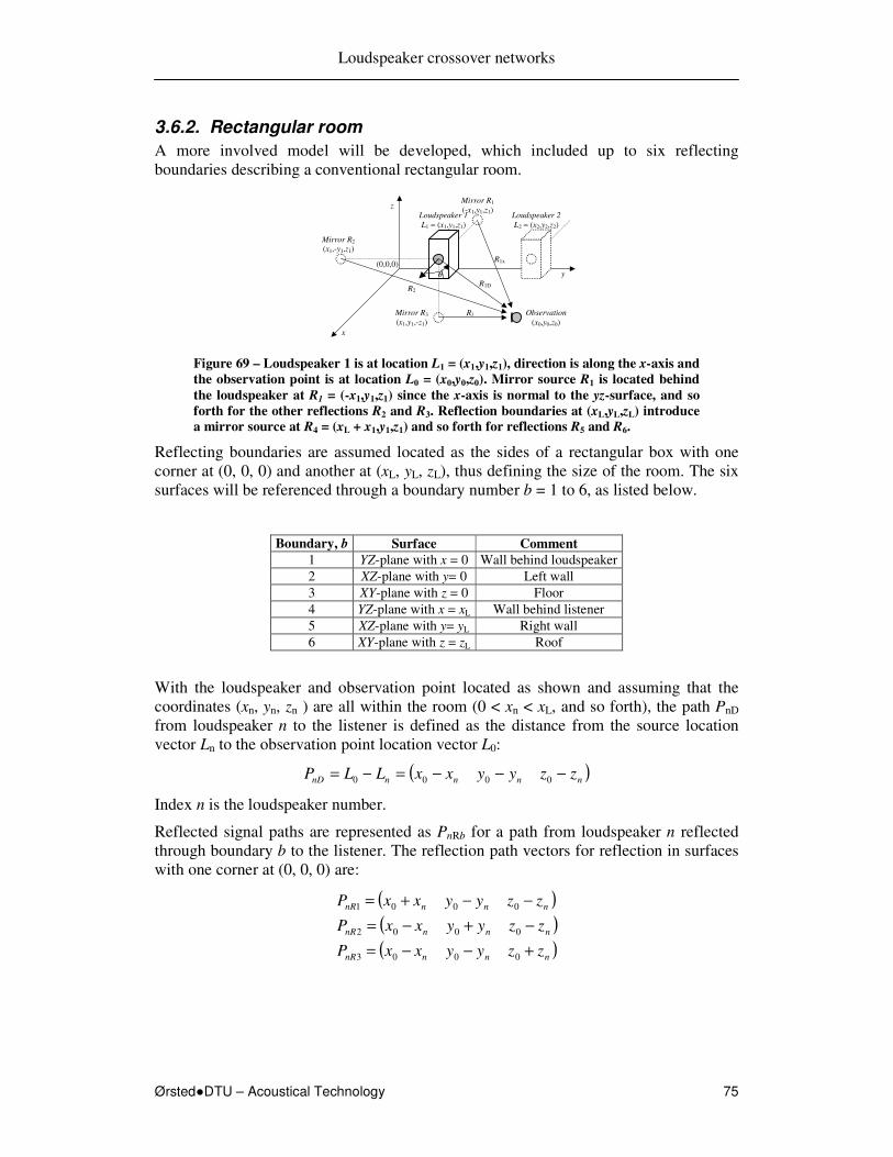
Loudspeaker crossover networks
ØrstedDTU – Acoustical Technology 75
3.6.2. Rectangular room
A more involved model will be developed, which included up to six reflecting boundaries describing a conventional rectangular room.
Loudspeaker 1
L1 = (x1,y1,z1)
Mirror R3
(x1,y1,-z1)
Observation
(x0,y0,z0)
x
y
z Mirror R1
(-x1,y1,z1)
Mirror R2
(x1,-y1,z1)
θ1
R1D
R1x
R2
R3
Loudspeaker 2
L2 = (x2,y2,z2)
(0,0,0)
Figure 69 – Loudspeaker 1 is at location L1 = (x1,y1,z1), direction is along the x-axis and
the observation point is at location L0 = (x0,y0,z0). Mirror source R1 is located behind
the loudspeaker at R1 = (-x1,y1,z1) since the x-axis is normal to the yz-surface, and so
forth for the other reflections R2 and R3. Reflection boundaries at (xL,yL,zL) introduce
a mirror source at R4 = (xL + x1,y1,z1) and so forth for reflections R5 and R6.
Reflecting boundaries are assumed located as the sides of a rectangular box with one corner at (0, 0, 0) and another at (xL, yL, zL), thus defining the size of the room. The six surfaces will be referenced through a boundary number b = 1 to 6, as listed below.
Boundary, b Surface Comment
1 YZ-plane with x = 0 Wall behind loudspeaker
2 XZ-plane with y= 0 Left wall
3 XY-plane with z = 0 Floor
4 YZ-plane with x = xL Wall behind listener
5 XZ-plane with y= yL Right wall
6 XY-plane with z = zL Roof
With the loudspeaker and observation point located as shown and assuming that the coordinates (xn, yn, zn ) are all within the room (0 < xn < xL, and so forth), the path PnD from loudspeaker n to the listener is defined as the distance from the source location vector Ln to the observation point location vector L0:
( )nnnnnD zzyyxxLLP −−−=−= 0000
Index n is the loudspeaker number.
Reflected signal paths are represented as PnRb for a path from loudspeaker n reflected through boundary b to the listener. The reflection path vectors for reflection in surfaces with one corner at (0, 0, 0) are:
( )( )( )nnnnR
nnnnR
nnnnR
zzyyxxP
zzyyxxP
zzyyxxP
+−−=−+−=−−+=
0003
0002
0001

Loudspeaker crossover networks
ØrstedDTU – Acoustical Technology 76
And for reflection in surfaces with one corner at (xL, yL, zL):
( )( )( )( )
( )( )nLnnnR
nnLnnR
nnnLnR
zzzyyxxP
zzyyyxxP
zzyyxxxP
−−−−=−−−−=−−−−=
2
2
2
0006
0005
0004
Loudspeaker radiation is dependent upon the angle from on-axis so the direction of the loudspeaker must be specified. Loudspeaker n is orientated with the main direction (loudspeaker front side) pointing along the direction vector LnD:
( )nDnDnDnD zyxL =
The coordinates can be determined from the horizontal angle θ, which is 0° along the x-
axis and the vertical angle φ, which is 0° at the xy-plane (z = 0), as:
( ) ( )( ) ( )( )nnD
nnnD
nnnD
z
y
x
φφθφθ
sin
cossin
coscos
===
For loudspeaker 1 pointing along the x-axis the vector becomes L1D =(1, 0, 0).
The observation angle is different for the reflections; one coordinate changes sign due to the reflection.
( )( )( )nDnDnDnRnR
nDnDnDnRnR
nDnDnDnRnR
zyxLL
zyxLL
zyxLL
−==−==
−==
63
52
41
The observation angle for the direct sound from the loudspeaker θnD is determined as the angle between the loudspeaker direction vector LnD and the vector pointing from the loudspeaker to the observation point PnD. The angle is 0° for the loudspeaker pointing directly at the observation point. The observation angle is extracted from the definition of the inner product (dot product) between LnD and PnD [5]:
( )nDnDnDnDnD PLPL θcos=•
The observation angle for the direct signal from loudspeaker n becomes:
•=
nDnD
nNnDnD
PL
PLarccosθ
The inner product is defined in MATLAB with A • B expressed as A’ * B, where A’ means the transposed of column vector A.
The observation angles for the reflections are:
•=
•=
•=
•=
•=
•=
66
666
55
555
44
444
33
333
22
222
11
111
arccosarccosarccos
arccosarccosarccos
nRnR
nRnRnR
nRnR
nRnRnR
nRnR
nRnRnR
nRnR
nRnRnR
nRnR
nRnRnR
nRnR
nRnRnR
PL
PL
PL
PL
PL
PL
PL
PL
PL
PL
PL
PL
θθθ
θθθ

Loudspeaker crossover networks
ØrstedDTU – Acoustical Technology 77
The sound pressure at the observation point from loudspeaker n and six reflections, assuming equal volume velocity Q for all loudspeakers and mirror sources, is:
( ) ( ) ( ) ( )∑=
−+−=6
1
exp4
exp4 b
nRbRbnRb
nRb
nDnD
nD
n DCikPP
QiDikP
P
Qip θ
πωρθ
πωρ
The reflection coefficient CR was included for two reasons; it is an easy way to selective enable and disable reflections and it allows use of partially reflective surfaces. Set all coefficients to zero to completely cancel reflection or set one or more to unity to selectively enable reflection. Values between zero and unity simulates panel absorbers, thick curtains or walls with large openings and the constants may be complex, if
required. D(θ) represents the loudspeaker directivity, which is defined in 3.3.
The resultant sound pressure from N loudspeakers with six reflecting surfaces:
( ) ( ) ( ) ( )∑ ∑= =
−+−=
N
n b
nRb
nRb
nRbbn
n
n ikPP
DCikP
P
DQip
1
6
1
expexp4
θθπ
ωρ
3.6.3. Home entertainment
A typical set-up for home entertainment could be with the loudspeaker 1 m above ground and the listener at 2 m distance and with the head at the same height as the loudspeaker.
1 m
2 m
Figure 70 – Set-up for home entertainment with a loudspeaker in a living room, which
was 5 m ×××× 10 m and 3 m high in the analysis.
The amplitude response is shown in Figure 71, left. The reflection is delayed 0.82 m corresponding to a half wave length at 210 Hz where destructive interference occurs. Lower frequencies are increased due to the reflection being in-phase and higher frequencies oscillates. An improvement for the low-frequency operation can be obtained by reducing the loudspeaker elevation as shown to the right.
The curves are similar to Figure 68, which was calculated using the simplified model with one reflecting boundary. The difference in Figure 71, right, is due to the loudspeaker pointing along the x-axis and not directly toward the listener.

Loudspeaker crossover networks
ØrstedDTU – Acoustical Technology 78
Figure 71 – Amplitude response for loudspeaker at 1 m height and 2 m distance (left)
and height reduced to 0.2 m (right). Listening height was 1 m. Diaphragm radius was
a = 0.1 m and the loudspeaker points along the x-axis.
The oscillations ceases at high frequencies due to the frequency-dependent loudspeaker directivity and the small bursts of oscillation at high frequency is caused by side lobes. Anyway, the model is not valid for high frequencies where the diaphragm is not vibrating as a rigid piston, the limit is around ka < 3, which is 1.6 kHz for a diaphragm diameter of a = 0.1 m.
Activating reflection from the side wall with 1 m distance from the loudspeaker and listener reintroduces the reflection with the dip at 210 Hz but the dip is less pronounced now since the overall level is increased. Moving the loudspeaker closer to the wall increases the frequency of the dip.
Figure 72 – Amplitude response for loudspeaker at 0.2 m height, 1 m from a wall and
at 2 m listener (left). Distance to wall reduced to 0.5m (right).
The high-frequency response is more ragged than before since three signal paths are combined (direct sound and two reflections). Activating the reflection from the wall behind the loudspeaker increases the low-frequency level.

Loudspeaker crossover networks
ØrstedDTU – Acoustical Technology 79
Figure 73 – Amplitude response for loudspeaker at 0.2 m height, 1 m from both walls
and at 2 m to listener (left). Distance to all three surfaces reduced to 0.2 m (right).
A descent amplitude response is obtained with the loudspeaker located close to both the corner between floor and walls as shown in Figure 73, right. The amplitude response indicates the need of crossover to the midrange loudspeaker below 200 Hz so the corner is optimal for a sub woofer (ignoring the standing waves within a real room).
The midrange and treble loudspeakers should be displaced from the sub woofer in order to reduce the effect of room reflections.
All surfaces are activated in Figure 74 where the loudspeaker is located at some distance from the corner at the left drawing and is moved closer to the corner in the second drawing. The most flat amplitude response is obtained close to the corner, but using the corner position may cause excitation of room resonances, not modelled here, and this may lead to a booming reproduction of low frequencies.
Figure 74 – Amplitude response for a room of 5 m by 10 m with 3 m height.
Loudspeaker at 1 m distance from corner (left) or 0.2 m from corner (right).
It is interesting to note, that the level at low frequencies is not increased 3 dB for each surface, as is sometimes stated in the popular literature; the figures are rather 6 dB from the first surface, 3 dB from the two next, and an insignificant amount from additional surfaces. There is no simple explanation to this observation – it could be expected that the direct and reflected signals would add almost lossless at low frequencies, but it appears not to be so.

Loudspeaker crossover networks
ØrstedDTU – Acoustical Technology 80
3.6.4. Public address
Another application is a large room for theatre or concerts, which is fitted with a loudspeaker system for public address.
1 m
2 m
Figure 75 – Large room for concerts, with dimensions 50 m ×××× 30 m and 15 m high.
The loudspeaker is located 5 m from each wall and 10 m above the floor and the
listening position was 35 m from the loudspeaker, 1/3 from the wall and 3 m above the
floor. The surfaces were absorbing.
The resulting amplitude response for a room with reflecting surfaces is shown in Figure 76 for a room without damping material. Only the direct signal and six reflections are included but the amplitude response is very ragged with ±10 dB variation within the main frequency range. The effect of adding damping to the surfaces is shown to the right, where the amplitude response is within ±5 dB for most of the audible range but the overall level is reduced some 10 dB since the reflections are reduced in level.
Figure 76 – Amplitude response for a room without damping (left) and the reflection
coefficients adjusted to 0.3 for the wall behind loudspeaker and the left and right walls
and 0.1 for roof, floor and the wall behind the listener (right).
The decaying high-frequency amplitude is caused by the directivity of the loudspeaker; the listener is off-axis.

Loudspeaker crossover networks
ØrstedDTU – Acoustical Technology 81
3.7. Loudspeaker characteristics
Four loudspeakers have been selected as being representative for the loudspeaker sizes found in two-way and three-way systems and are listed in Table 3 together with the published parameters of interest for this study. The values are not directly used in this document but have formed the basis for selection of parameters.
Table 3 – Typical loudspeaker characteristics for two-way and three-way systems.
Loudspeaker model P:Peerless, S:ScanSpeak
Symbol Woofer S:26W8667
Bass P:205WR33
Midrange S:13M8636
Treble S:DT2905
Unit
Diaphragm diameter D 168 mm
Effective diaphragm area SD 32 10-3 22 10-3 4.8 10-3 0.85 10-3 m2
Voice coil resistance RE 5.8 6.0 5.8 4.7 Ω
Voice coil inductance LE 0.4 1.8 0.1 0.08 mH
Force factor BL 11.1 9.6 6.0 3.5 N/A
Diaphragm & voice coil mass MMD 56 25.9 4.6 0.45 g
Suspension compliance CMS - 1.13 - - mm/N
Suspension friction loss RMS 1.5 - 0.8 - kg/s
Sensitivity (2.83 V) Lref 87 90 86.5 90 dB
Linear excursion xMAX ±9.0 ±5.5 ±1.5 ±0.4 mm
Electrical quality factor QMS 5.2 3.94 2.8 - -
Mechanical quality factor QES 0.36 0.31 0.36 - -
Total quality factor QTS 0.34 0.29 0.32 - -
Equivalent volume VAS 136 76 3.0 - m3
Resonance frequency fS 22 30 77 650 Hz
Frequency for ka = 1 fA 0.54 1.4 3.3 kHz
Frequency due to voice coil fC 2.3 9.2 9.4 kHz
The top values refers to the published figures for the stated loudspeakers. The bottom two values are calculated using the equations from this section.

Loudspeaker crossover networks
ØrstedDTU – Acoustical Technology 82
3.8. Group delay
Group delay specify the delay experienced by a group of sinusoidal components, which
have frequencies within a narrow frequency interval about f = ω/2π. The bandwidth in this interpretation must be restricted to a frequency interval over which the phase response is approximately linear.
3.8.1. Calculation method
The group delay is defined as the rate of change of phase with respect to frequency [7]:
ωθτ
d
dGD −=
The phase is a property of the transfer function H(ω), which can be written in polar
notation with G(ω) as the amplitude response and θ(ω) as the phase response where both are real valued functions:
( ) ( ) ( )( )ωθωω iGH exp=
This can be separated into amplitude and phase terms using the logarithmic function.
( )( ) ( )( ) ( )ωθωω iGH += lnln
This is differentiated with respect to angular frequency:
( )( ) ( )( ) ( )ωθω
ωω
ωω d
diG
d
dH
d
d+= lnln
Using the differentiation rule for the logarithm (Schaum 13.27):
( )( )
( )( ) ( )ωθωω
ωω
'''
iG
G
H
H +=
G’(ω) and θ’(ω) denotes the derivative of G(ω) and θ(ω) respectively. The group delay
is represented by the imaginary part, and since G’(ω)/G(ω) is real this becomes.
( ) ( )( )
−=−=ωωωθτ
H
HGD
'Im'
3.8.2. Implementation in MATLAB
The derivative of H(ω) can be expressed as the slope of H(ω) within a narrow frequency
range from ω to ω + ∆ω by use of the definition of the derivative (Schaum 13.1):
( ) ( ) ( )ω
ωωωωω ∆
−∆+=
→∆
HHH
0lim'
The difference ∆ω cannot reach zero so a finite value of 0.001 will be used.
The frequency variable is s0 = iω/ω0 = if/f0 so the increment becomes ∆ω = 0.001ω0 or
alternatively ∆f = 0.001f0. The incremental frequency is thus 1 Hz for a normalisation frequency (crossover frequency) of f0 = 1000 Hz.

Loudspeaker crossover networks
ØrstedDTU – Acoustical Technology 83
Hence, calculation of H(ω) using the following expression:
( ) ( ) ( )( )
∆−∆+
−=−=ωω
ωωωωθτH
HHGD Im'
The frequency is defined as the vector f0*[0.1:0.001:10], using MATLAB notation, so the incrementally larger frequency uses another vector g defined from f to output the step following immediately after, i.e. defined as g = f + 0.001* f0.
3.8.3. Verification
Two filters will be analysed for testing the MATLAB implementation of group delay.
The first test object is a first-order low-pass filter, which is brought onto a form suitable for analytic extraction of the phase.
2
0
0
00
0
0
0
1
1
1
11
1
1
1
1
1
+
−=
−
+
−=
+=
+=
ωω
ωω
ωω
ωω
ωω
ωω
i
ii
i
isH
The phase is:
01
1
Re
Imarctan
ωωθ i
H
H−=
=
And the group delay becomes (Schaum 13.22):
2
0
001
11
+
=
−−=
ωωωω
ωω
τ id
dGP
The result is shown in Figure 77 and indicates good agreement.
Figure 77 – Group delay using the analytic expression (left) and the calculation from
the transfer function of the low-pass filter (right).

Loudspeaker crossover networks
ØrstedDTU – Acoustical Technology 84
The second test object a second-order all-pass filter with constant amplitude for a1 = 2.
2
001
2
02
1
1
ssa
sH
++−
=
The derivative of the test function can be calculated from the definition of the derivative of a quotient of two functions (Schaum 13.9):
( ) ( ) ( ) ( )( )22
001
2
001
2
0
2
0
2
0012
2
1
1111'
ssa
ssad
dss
d
dssa
d
dHH
++
++−−−++== ωω
ω
The derivative of the frequency variables:
( )
( ) 0
000
2
0
2
0
2
0
00
0
222s
iiii
d
ds
d
d
ii
d
ds
d
d
ωωω
ωωω
ωω
ωω
ωωω
ωω
==−=
=
=
=
Hence, the derivative of the test function:
( ) ( )( )22
001
0
00
12
00
0
2
001
2
1
21
21
'ssa
siia
ssi
ssa
H++
+−−
−++
=ωωω
This was implemented in MATLAB for comparison and the result of the analytical expression is shown in Figure 78 with the calculation method based on transfer function output shown in Figure 79.
Figure 78 – Group delay using a test function with symbolic differentiation carried
out before calculation. Plot for a1 = 1 (left) and a1 = 2 (right).

Loudspeaker crossover networks
ØrstedDTU – Acoustical Technology 85
Figure 79 – Group delay using the transfer function output at two frequencies with
incremental distance (i.e. f and f + ∆∆∆∆f). Plot for a1 = 1 (left) and a1 = 2 (right).
There are no visual differences between the figures, so the agreement is good. But a couple of figures using some few transfer functions cannot proof the validity of the calculation – but it indicates that the method come close on a couple of tests.

Loudspeaker crossover networks
ØrstedDTU – Acoustical Technology 86
4. Assembling the models It is time to combine the models into a system design trial. The target is a low-budget two-way system, so the design must be kept simple and uncomplicated to assemble during production, i.e. using a simple passive crossover network.
4.1. Loudspeaker models
The loudspeaker system is a closed cabinet with baffle measures shown in Figure 88. The loudspeaker units are:
• A bass loudspeaker, 8 inch with 70 Hz resonance frequency and a total quality factor of 0.7 within the cabinet and it is assumed to reproduce smoothly to 3 kHz at –3 dB with a cut-off slope of –6 dB/octave at higher frequencies.
• A treble loudspeaker, 1 inch dome with 1 kHz resonance frequency, a total quality factor of 1 and high-frequency roll-off above 20 kHz at – 3 dB.
The amplitude and phase responses of the system are shown in Figure 80 where the “total” curve represents a system where the outputs are added without a crossover filter.
Figure 80 – Loudspeaker models for the two-way system. The bass loudspeaker is
defined by the resonance frequency fS = 70 Hz, total quality factor QTC = 0.7 and high-
frequency roll-off at fC = 3 kHz. For the treble loudspeaker is fS = 1 kHz, QTC = 1.0
and fC = 20 kHz.
4.2. Crossover network
A crossover network must protect the treble loudspeaker, and this is in this report assumed fulfilled for at least 20 dB of attenuation at the resonance frequency of 1 kHz. Using a second-order crossover network offers 24 dB of attenuation with a crossover frequency of 4 kHz, so this will be used for a start.
A notch at the crossover frequency is to be expected using a second-order crossover network due to 180° of phase difference between the bass and treble loudspeakers so the treble loudspeaker is inverted. Assuming ideal addition of the outputs require a crossover network with 6 dB attenuation at the crossover frequency so the filter must use a quality factor of 0.5 since the attenuation is 20 log10(Q) dB.
The resulting amplitude and phase responses are shown in Figure 81. A dip of approximately 3 dB is seen at the crossover frequency.

Loudspeaker crossover networks
ØrstedDTU – Acoustical Technology 87
Figure 81 – Resultant amplitude and phase response for the system with a second-
order crossover network at 4 kHz and inverted treble.
The phase difference between bass and treble is around 50°, so the loudspeakers are not in-phase due to the phase responses of the loudspeaker units. The difference can be reduced by removing one of the poles from the low-pass filter thus simplifying the crossover network by reducing the low-pass filter to first order. The result is shown in Figure 82, where the phase difference is close to 0° at 4 kHz and the amplitude response is improved.
Figure 82 – Loudspeaker response for a system with a first-order low-pass filter for
the bass loudspeaker and second-order filter for the treble loudspeaker.
A crossover network with an inductor in series with the loudspeaker is not attractive, first of all due to the loudspeaker impedance, which is increasing at high frequencies and thus opposing the intended low-pass filtering, and second, because the inductor is a relatively costly component.
Bass
REB
CT1
Treble
RET LT1
Figure 83 – Passive crossover network for the two-way system. The bass loudspeaker
high-frequency roll-off is used as the low-pass channel of the crossover network.

Loudspeaker crossover networks
ØrstedDTU – Acoustical Technology 88
If the inductor is removed, the resulting crossover network consists of a second-order high-pass filter for the treble loudspeaker and no filter for the bass loudspeaker. This is very attractive from a production point of view, but the resulting response in Figure 84 (left picture) shows response peaking some 2 dB around the crossover frequency. This peak will not be removed by the inductor, unless an impedance compensation is included for the bass loudspeaker, and this is not the idea behind the system.
Figure 84 – Loudspeaker response with the low-pass filter removed (left) and with the
treble loudspeaker attenuated 6 dB (right). Neither designs are acceptable.
The peak can be removed by attenuation of the treble loudspeaker, but the resultant amplitude response, shown in Figure 84 (right picture), shows that the result is an early roll-off in the treble, which cannot be accepted.
The phase response of the bass channel should include two poles, one from the loudspeaker and another from the crossover network, but the current design only includes the pole from the loudspeaker. The phase is not sufficiently negative, so it could be possible to add the missing phase by time-shifting of the signal from the treble loudspeaker by moving it axially. A time shift introduces a rotating phase where the
angular speed is defined by frequency f and the distance ∆L the treble loudspeaker is moved, according to:
( )c
LfiH DDTIME
∆=−= ττ ,exp
A delay of 100 µs corresponds to a distance of ∆L = 34 mm and the result of this movement of the treble loudspeaker is shown to the left in Figure 85. The result is not the intended removal of the peak, rather is the amplitude response completely ruined by the movement. Doing the opposite, advancing time by moving the treble loudspeaker toward the listener, is shown to the right is Figure 85. There is a little change but the peak is not at all removed.
So, it seems that we have to live with the 2 dB boost around 4 kHz.

Loudspeaker crossover networks
ØrstedDTU – Acoustical Technology 89
Figure 85 – Loudspeaker response with loudspeaker delayed 100 µµµµs by moving is 34
mm into the cabinet, or the bass loudspeaker 34 mm out from the cabinet (left) and
advancing the time 100 µµµµm by moving it the other way (right).
4.3. Angular response
The loudspeaker proved rather sensitive to modest delays, thus indicating that it would be a good idea to study the behaviour to off-axis listening. Two angles are relevant for this analysis, the horizontal angle representing a loudspeaker pointing toward one of the sides of the head of the listener, and the vertical angle representing a loudspeaker pointing above or below the head.
The effect of horizontal angle is shown in Figure 86 for two angles at 15° and 30° and shows that the amplitude response is somewhat sensitive to changes in the horizontal angle. The bass loudspeaker is the problem since the diaphragm diameter is comparable to wavelengths around the crossover frequency.
Figure 86 – Loudspeaker response for a horizontal angle of 15° (left) and 30° (right).
The loudspeakers radius was 100 mm for the bass loudspeaker and 10 mm for the
treble loudspeaker. The bass loudspeaker becomes directive above 550 Hz (ka = 1).
The effect of vertical angle is shown in Figure 87 for two angles at 15° and 30° and shows that the amplitude response is quite sensitive to changes in the horizontal angle. The loudspeaker is not symmetrical on the vertical axis, and the behaviour for negative angles is not shown here, but the curves indicate that the loudspeaker must be tilted so that it points to the listener.

Loudspeaker crossover networks
ØrstedDTU – Acoustical Technology 90
Figure 87 – Loudspeaker response for a vertical angle of 15° (left) and 30° (right).
A conclusion so far is that the peak at the crossover frequency should be kept as it is although the on-axis response could be improved. The consequence of modifying the loudspeaker to a flatter amplitude would most probably be degradation of the off-axis response. The direct sound will be slightly improved around the crossover frequency but the off-axis response shows a decrease in the same range and this affects the sound pressure level within the reverberant field.
4.4. Reflections
Reflection from the edges of the loudspeaker interferes with the loudspeaker and was modelled in section 3.4 where the model with circular sections were most successful and will be used for the analysis below. The loudspeaker cabinet is rectangular and will be modelled by four circular sections with radii equal to the mean distance from the centre of the bass loudspeaker to the edge. This is a coarse model, but it gives an idea of the effect of the front baffle.
L
200 mm H
400 mm
W
250 mm
150 mm
D1
150 mm D2
210 mm
D4
290 mm
D5
250 mm
D3
150 mm
Figure 88 – Loudspeaker front baffle measures for calculation of diffraction.
The shortest mean distance is the average between D1 and D2; hence R1 = 0.18 m. Due to symmetry is the two next shortest distances identical and the average between D2, D3 and D4; hence R2 = R3 = 0.22 m. The largest mean distance is the average between D4 and D5; hence R1 = 0.27 m. The result is shown in Figure 89 and is seen to overrule the effect of the peak around the crossover frequency. Also seen is the reduced output at low frequencies where the baffle becomes small compared to wavelength. The
loudspeaker is at low frequencies radiating into 4π solid angle, while the baffle limits
the radiation angle to 2π at higher frequencies.

Loudspeaker crossover networks
ØrstedDTU – Acoustical Technology 91
Figure 89 – Loudspeaker response with reflections from the baffle (left) and with
reflections from one boundary included (right). The loudspeaker was located 1 m
above ground at 2 m distance from the listener.
Reflections from a large surface (the floor) is shown to the right of Figure 89 with the loudspeaker 1 m above ground at 2 m distance to the listener with his or hers ears 1 m above ground. The low frequency response is improved but a dip is seen at 210 Hz, which is due to the delayed distance through the reflection path, which is 0.83 m longer than the direct path and cause destructive interference with the direct signal. Interference becomes constructive at 420 Hz and so forth.
Figure 90 – Loudspeaker at 0.5 m (left) and 0.25 m (right). The model includes the
crossover network, the loudspeakers, diffraction and one reflection.
An improvement is obtained by reducing the loudspeaker height to 0.5 m above the floor (Figure 90, left picture). The first dip occur at 350 Hz and the first peak is located at 700 Hz. The peak is of large amplitude but can be reduced by lowering the height to 0.25 m above the floor (Figure 90, right picture).
The high-frequency ripple is due to the simplified models and will be less pronounced in real life.
4.5. Conclusion
The models form an effective tool for initial loudspeaker design although improvements are required especially for the diffraction and boundary reflection models.

Loudspeaker crossover networks
ØrstedDTU – Acoustical Technology 92
5. References
5.1. Books
[1]: Brian C. J. Moore “An introduction to the Psychology of Hearing”, 5th edition, 2004, Elsevier Academic Press.
[2]: W: Marshall Leach, Jr. “Introduction to Electroacoustics & Audio Amplifier Design”, 3rd edition, 2003, Kendall/Hunt Publishing Company.
[3]: Leo L. Beranek, “Acoustics”, Acoustical Society of America, 1993 edition, 1996.
[4] Finn Jacobsen, Peter Juhl “Radiation of Sound”, not published, DTU, 2005.
[5] Hans Ebert “Elektronik Ståbi”, Teknisk Forlag, 1995.
[6] http://ccrma.stanford.edu/~jos/filters/Group_Delay.html.
5.2. Papers
Paper: S. Linkwitz, 'Active Crossover Networks for Non-Coincident Drivers,' J. Audio
Eng. Soc., vol. 24, pp. 2-8 (Jan./Feb. 1976) – together with his co-worker Russ Riley
5.3. Links
http://sound.westhost.com/lr-passive.htm - A very nice introduction to the design of a crossover network, including compensation of loudspeaker impedance, voice coil temperature and much more.

Loudspeaker crossover networks
ØrstedDTU – Acoustical Technology 93
6. Appendix
6.1. Plot transfer function
Amplitude and phase responses are plotted using the following MATLAB shell script. Representative functions addressed within the script are included in the following section.
6.1.1. Main script
The file was executed by entering plot_transfer_function at the MATLAB prompt.
% Plot transfer functions.
clear all % Remove old stuff.
% -------------------------------------------------------------------------
% Constants.
% -------------------------------------------------------------------------
% Frequency.
FBEG = 20; % Start frequency (Hz).
FEND = 20000; % Stop frequency (Hz).
FSTEP = 1; % Frequency increment (Hz).
f = [FBEG:FSTEP:FEND]; % Frequency f.
g = f + FSTEP; % Frequency g (required for group delay).
% Acoustical.
F0 = 4000; % Crossover frequency (Hz).
c = 343; % Speed of sound (m/s).
L = 0.25; % Displacement between loudspeakers (m).
% Miscellaneous.
D2R = pi/180; % Conversion from degrees to radians.
R2D = 180/pi; % Conversion from radians to degrees.
TRUE = logical(1); % Used by the IF statement.
FALSE = logical(0);
% -------------------------------------------------------------------------
% Crossover network coefficients.
% -------------------------------------------------------------------------
% Second order, N = 2:
A1 = 2.00; % 1.00
% Third order, N = 3:
% A1 = 3.00;
% A2 = 3.00;
% Fourth order, N = 4:
% A1 = 2.83; % 2.00, 2.61
% A2 = 4.00; % 3.00, 3.41
% A3 = 2.83; % 2.00, 2.61
% Sixth order, N = 6:
% A1 = 1.00;
% A2 = 3.00;
% A3 = 6.00;
% A4 = 3.00;
% A5 = 1.00;
% -------------------------------------------------------------------------
% Crossover network at frequency f.
% -------------------------------------------------------------------------
bass_f = 1;
% treble_f = 1;

Loudspeaker crossover networks
ØrstedDTU – Acoustical Technology 94
% bass_f = lowpass_1(F0,f);
% treble_f = highpass_1(F0,f);
% bass_f = lowpass_2(F0,A1,f);
% midrange_f = bandpass_2(F0,A1,f);
treble_f = highpass_2(F0,A1,f);
% bass_f = lowpass_3(F0,A1,A2,f);
% midrange_f = bandpass_3(F0,A1,A2,f);
% treble_f = highpass_3(F0,A1,A2,f);
% bass_f = lowpass_4(F0,A1,A2,A3,f);
% midrange_f = bandpass_4(F0,A1,A2,A3,f);
% treble_f = highpass_4(F0,A1,A2,A3,f);
% bass_f = lowpass_6(F0,A1,A2,A3,A4,A5,f);
% treble_f = highpass_6(F0,A1,A2,A3,A4,A5,f);
% -------------------------------------------------------------------------
% Crossover network at frequency g.
% -------------------------------------------------------------------------
bass_g = 1;
% treble_g = 1;
% bass_g = lowpass_1(F0,g);
% treble_g = highpass_1(F0,g);
% bass_g = lowpass_2(F0,A1,g);
% midrange_g = bandpass_2(F0,A1,g);
treble_g = highpass_2(F0,A1,g);
% bass_g = lowpass_3(F0,A1,A2,g);
% midrange_g = bandpass_3(F0,A1,A2,g);
% treble_g = highpass_3(F0,A1,A2,g);
% bass_g = lowpass_4(F0,A1,A2,A3,g);
% midrange_g = bandpass_4(F0,A1,A2,A3,g);
% treble_g = highpass_4(F0,A1,A2,A3,g);
% bass_g = lowpass_6(F0,A1,A2,A3,A4,A5,g);
% treble_g = highpass_6(F0,A1,A2,A3,A4,A5,g);
% -------------------------------------------------------------------------
% Include loudspeaker models.
% -------------------------------------------------------------------------
% Treble loudspeaker.
FCT = 20e3; % Voice coil cutoff pole frequency (Hz).
FLT = 10e6; % Voice coil cutoff null frequency (Hz).
FST = 1e3; % Mechanical resonance frequency (Hz).
QTCT = 1; % Total quality factor.
treble_f = loudspeaker(FCT,FLT,FST,QTCT,treble_f,f);
treble_g = loudspeaker(FCT,FLT,FST,QTCT,treble_g,g);
% Midrange loudspeaker.
FCM = 10e3; % Voice coil cutoff pole frequency (Hz).
FLM = 10e6; % Voice coil cutoff null frequency (Hz).
FSM = 100; % Mechanical resonance frequency (Hz).
QTCM = 1; % Total quality factor.
% midrange_f = loudspeaker(FCM,FLM,FSM,QTCM,midrange_f,f);
% midrange_g = loudspeaker(FCM,FLM,FSM,QTCM,midrange_g,g);
% Bass loudspeaker.
FCB = 3e3; % Voice coil cutoff pole frequency (Hz).
FLB = 10e6; % Voice coil cutoff null frequency (Hz).
FSB = 70; % Mechanical resonance frequency (Hz).
QTCB = 0.7; % Total quality factor.
bass_f = loudspeaker(FCB,FLB,FSB,QTCB,bass_f,f);
bass_g = loudspeaker(FCB,FLB,FSB,QTCB,bass_g,g);
% -------------------------------------------------------------------------
% Introduce directivity.
% -------------------------------------------------------------------------
THETA = 0; % Horisontal or vertical ongle (degrees).
AT = 10e-3; % Treble diaphragm radius (m).
AM = 50e-3; % Midrange diaphragm radius (m).
AB = 100e-3; % Bass diaphragm radius (m).

Loudspeaker crossover networks
ØrstedDTU – Acoustical Technology 95
% treble_f = directivity(THETA,AT,f).*treble_f;
% treble_g = directivity(THETA,AT,g).*treble_g;
% midrange_f = directivity(THETA,AM,f).*midrange_f;
% midrange_g = directivity(THETA,AM,g).*midrange_g;
% bass_f = directivity(THETA,AB,f).*bass_f;
% bass_g = directivity(THETA,AB,g).*bass_g;
% -------------------------------------------------------------------------
% Introduce phase due to vertical angle.
% -------------------------------------------------------------------------
% Vertical offset angle.
VA = 0; % Vertical offset angle (degrees).
% Two-loudspeaker arrangement (bass + treble).
% treble_f = exp( i*2*pi*f*L*sin(VA*D2R)/(2*c)).*treble_f;
% treble_g = exp( i*2*pi*g*L*sin(VA*D2R)/(2*c)).*treble_g;
% bass_f = exp(-i*2*pi*f*L*sin(VA*D2R)/(2*c)).*bass_f;
% bass_g = exp(-i*2*pi*g*L*sin(VA*D2R)/(2*c)).*bass_g;
% midrange_f = midrange_f;
% midrange_g = midrange_g;
% Three-loudspeaker arrangement (bass + treble + bass).
% treble_f = treble_f;
% treble_g = treble_g;
% bass_f = (exp( i*2*pi*f*L*sin(VA*D2R)/c) + ...
% exp(-i*2*pi*f*L*sin(VA*D2R)/c)).*bass_f/2;
% bass_g = (exp( i*2*pi*g*L*sin(VA*D2R)/c) + ...
% exp(-i*2*pi*g*L*sin(VA*D2R)/c)).*bass_g/2;
% -------------------------------------------------------------------------
% Resultant transfer functions.
% -------------------------------------------------------------------------
ATT = 1.0; % Attenuator network.
DLY = 0e-6; % Delay (s).
% sum_f = bass_f + treble_f; % Two-way.
% sum_g = bass_g + treble_g;
sum_f = bass_f - ATT*treble_f; % Two-way, inverted.
sum_g = bass_g - ATT*treble_g;
% sum_f = bass_f - treble_f.*exp(-i*f*DLY); % Two-way, time shifted.
% sum_g = bass_g - treble_g.*exp(-i*f*DLY);
% sum_f = bass_f + midrange_f + treble_f; % Three-way.
% sum_g = bass_g + midrange_g + treble_g;
% sum_f = ones(size(f)); % Dummy (unity sums).
% sum_g = ones(size(g));
% -------------------------------------------------------------------------
% Include diffraction model.
% -------------------------------------------------------------------------
sum_f = diffraction_sectional(0.18,0.22,0.22,0.27, f).*sum_f;
sum_g = diffraction_sectional(0.18,0.22,0.22,0.27, f).*sum_g;
% -------------------------------------------------------------------------
% Include one-dimensional boundary reflection model.
% -------------------------------------------------------------------------
H1 = 0.25; % Loudspeaker distance above floor (m).
H0 = 1.00; % Listener distance above floor (m).
L = 2.00; % Horizontal distance to listener (m).
RD = sqrt((H0 - H1)^2 + L^2);
RR = sqrt((H0 + H1)^2 + L^2);
TH = R2D*(atan((H0 - H1)/L) + atan((H0 + H1)/L));
sum_f = boundary_simple(RD,RR,TH,AB,f).*sum_f;
% -------------------------------------------------------------------------
% Plot amplitude spectrum.

Loudspeaker crossover networks
ØrstedDTU – Acoustical Technology 96
% -------------------------------------------------------------------------
figure(1);
semilogx(f, 20*log10(abs(sum_f)), ...
f, 20*log10(abs(treble_f)), ...
f, 20*log10(abs(bass_f)));
legend('Total','Treble','Bass');
axis([FBEG FEND -20 5]);
ylabel('Amplitude (dB)');
xlabel('Frequency (Hz)');
% -------------------------------------------------------------------------
% Plot phase spectrum.
% -------------------------------------------------------------------------
figure(2);
semilogx(f, R2D*angle(sum_f), ...
f, R2D*angle(treble_f), ...
f, R2D*angle(bass_f));
legend('Total','Treble','Bass');
axis([FBEG FEND -200 200]);
ylabel('Phase (°)');
xlabel('Frequency (Hz)');
% -------------------------------------------------------------------------
% Plot group delay spectrum.
% -------------------------------------------------------------------------
% Group delay = -Im(H'/H).
% groupdelay = -imag((sum_g - sum_f)./(sum_f*FSTEP));
% figure(3);
% semilogx(f, groupdelay);
% axis([FBEG FEND 0 1e-3]);
% ylabel('Group delay (s)');
% xlabel('Frequency (Hz)');
6.1.2. Filter function
All filters, being low-pass, band-pass or high-pass, are written in the below style. Input “f0” is the centre frequency of the filter and A1 and so forth are coefficients to the polynomials and are specified from the main script file. Input “f” is a frequency vector, either from 0.1 to 10 in steps of 0.01 (normalised frequency) or from 20 Hz to 20000 Hz in steps of 1 Hz. Different filter flavours are specified for several filters but only one is enabled by un-commenting the relevant definition.
% Second order low-pass filter.
function out = lowpass_2(f0,A1, f);
s0 = (i/f0)*f;
% out = (1 + A1*s0)./(1 + A1*s0 + s0.^2);
% out = (1 + (A1/2)*s0)./(1 + A1*s0 + s0.^2);
out = 1./(1 + A1*s0 + s0.^2);
Only the last equation is enabled.
6.1.3. Loudspeaker
A loudspeaker is defined by a second-order high-pass filter and a first-order low-pass filter. Input coefficients are specified from the main script. Variable in is the input response, which is returned with the loudspeaker transfer function.

Loudspeaker crossover networks
ØrstedDTU – Acoustical Technology 97
% Loudspeaker transfer function.
function out = loudspeaker(FC, FL, FS, QTC, in, f);
% FC = Voice coil pole frequency due to RE and LE (Hz).
% FL = Voice coil null frequency due to eddy currents (Hz).
% FS = Mechanical resonance frequency (Hz).
% QTC = Total quality factor.
out = ((1+i*f/FL)./(1+i*f/FC)) .* ...
( ((i*f/FS).^2)./(1+i*f/(FS*QTC)+(i*f/FS).^2) ).*in;
6.1.4. Directivity
Directivity is defined by the Bessel-function besselj, which is of the first kind. The if-statement avoids division by zero at low frequencies and zero angle.
function out = directivity(T, A, f)
% T = Angle (degrees).
% A = Loudspeaker radius (m).
% f = Frequency (Hz).
TT = (pi/180)*T; % Convert angle from degrees to radians.
ka = 2*pi*f*A/343; % Angular wave number.
out = ones(size(f));
if (abs(TT) > eps)
out = abs(2*besselj(1,ka*sin(TT))./(ka*sin(TT)));
end
6.1.5. Diffraction
A simplified model is used, which is based upon the circular section method, here limited to four sections (90° each).
function out = diffraction_sectional(R1,R2,R3,R4, f)
% R1 = Radius of section 1 (m).
% R2 = Radius of section 2 (m).
% R3 = Radius of section 3 (m).
% R4 = Radius of section 4 (m).
ikR1 = i*2*pi*f*R1/343;
ikR2 = i*2*pi*f*R2/343;
ikR3 = i*2*pi*f*R3/343;
ikR4 = i*2*pi*f*R4/343;
out = 1-( exp(-ikR1)+exp(-ikR2)+exp(-ikR3)+exp(-ikR4) )/8;
6.1.6. Boundary reflections
A simplified model is used for reflection from the boundary, which is only using one reflecting surface. The model includes loudspeaker directivity and assumes that the loudspeaker is pointing directly toward the listener.
function out = boundary_simple(RD,RR,TH,A,f);
% PD = Direct path length (m).

Loudspeaker crossover networks
ØrstedDTU – Acoustical Technology 98
% PR = Reflected path length (m).
ik = i*2*pi*f/343;
out = 1 + (RD/RR)*directivity(TH,A,f).*exp(-ik*(RR-RD));
6.2. Plot boundary reflection
This is the full script for calculation of the effect of boundary reflections. The model assume a rectangular room with six reflecting surfaces. The initial part of the script checks for negative or too large coordinates and zero diaphragm diameter.
% Compute the resultant sound pressure for a loudspeaker within a room.
clear all;
% -------------------------------------------------------------------------
% Input parameters.
% -------------------------------------------------------------------------
% Room dimensions (m):
XL = 50; YL = 30; ZL = 15;
% Observation point (m):
X0 = 40; Y0 = 10; Z0 = 3;
%Loudspeaker 1 (m):
X1 = 5; Y1 = 5; Z1 = 10;
A1H = 0; % Loudspeaker horisontal angle (degrees).
A1V = 0; % Loudspeaker vertical angle (degrees).
C1 = 0.3; % Reflection coefficient for wall behind loudspeaker (m).
C2 = 0.3; % Reflection coefficient for left wall (m).
C3 = 0.1; % Reflection coefficient for floor (m).
C4 = 0.1; % Reflection coefficient for wall behind listener (m).
C5 = 0.3; % Reflection coefficient for right wall (m).
C6 = 0.1; % Reflection coefficient for roof (m).
A = 0.1; % Loudspeaker diaphragm radius (m).
f = [10:1:10000]; % Frequency range.
% -------------------------------------------------------------------------
% Check consistency of input parameters.
% -------------------------------------------------------------------------
if (min([X0 Y0 Z0 X1 Y1 Z1]) < 0)
error('Coordinates (x,y,z) must not be negative.');
end
if (min([XL YL ZL]) < 0)
error('Room coordinates must not be negative.');
end
if (min([(XL-X0) (YL-Y0) (ZL-Z0) (XL-X1) (YL-Y1) (ZL-Z1)]) < 0)
error('oordinates (x,y,z) must not exceed room limits.');
end
if (min([C1 C2 C3 C4 C5 C6]) < 0)
error('Reflection coefficients (C) must not be negative.');
end
if (max([C1 C2 C3 C4 C5 C6]) > 1)
error('Reflection coefficients (C) must be maximum unity.');
end
if (A <= 0)
error('Loudspeaker diaphragm diameter must be positive.');
end
% -------------------------------------------------------------------------
% Calculate constant vectors.

Loudspeaker crossover networks
ØrstedDTU – Acoustical Technology 99
% -------------------------------------------------------------------------
% Distance vectors for loudspeaker 1:
P1D = [(X0-X1) (Y0-Y1) (Z0-Z1)]; % Direct signal.
P1R1 = [(X0+X1) (Y0-Y1) (Z0-Z1)]; % Reflection 1.
P1R2 = [(X0-X1) (Y0+Y1) (Z0-Z1)]; % Reflection 2.
P1R3 = [(X0-X1) (Y0-Y1) (Z0+Z1)]; % Reflection 3.
P1R4 = [(X0-(2*XL-X1)) (Y0-Y1) (Z0-Z1)]; % Reflection 4.
P1R5 = [(X0-X1) (Y0-(2*YL-Y1)) (Z0-Z1)]; % Reflection 5.
P1R6 = [(X0-X1) (Y0-Y1) (Z0-(2*ZL-Z1))]; % Reflection 6.
% Loudspeaker direction vector:
L1X = cos(pi*A1H/180)*cos(pi*A1V/180); % Coordinate x.
L1Y = sin(pi*A1H/180)*cos(pi*A1V/180); % Coordinate y.
L1Z = sin(pi*A1V/180); % Coordinate z.
L1D = [ L1X L1Y L1Z];
L1R1 = [-L1X L1Y L1Z];
L1R2 = [ L1X -L1Y L1Z];
L1R3 = [ L1X L1Y -L1Z];
L1R4 = [-L1X L1Y L1Z];
L1R5 = [ L1X -L1Y L1Z];
L1R6 = [ L1X L1Y -L1Z];
% -------------------------------------------------------------------------
% Observation angles:
% -------------------------------------------------------------------------
T1 = acos((L1D *P1D') /(norm(L1D) *norm(P1D))); % Direct signal.
T1R1 = acos((L1R1*P1R1')/(norm(L1R1)*norm(P1R1))); % Reflection 1.
T1R2 = acos((L1R2*P1R2')/(norm(L1R2)*norm(P1R2))); % Reflection 2.
T1R3 = acos((L1R3*P1R3')/(norm(L1R3)*norm(P1R3))); % Reflection 3.
T1R4 = acos((L1R4*P1R4')/(norm(L1R4)*norm(P1R4))); % Reflection 4.
T1R5 = acos((L1R5*P1R5')/(norm(L1R5)*norm(P1R5))); % Reflection 5.
T1R6 = acos((L1R6*P1R6')/(norm(L1R6)*norm(P1R6))); % Reflection 6.
% Check that the angls are non-zero (>2.2e-16) to avoid division by zero.
if (abs(T1)<eps) T1 = eps; end
if (abs(T1R1)<eps) T1R1 = eps; end
if (abs(T1R2)<eps) T1R2 = eps; end
if (abs(T1R3)<eps) T1R3 = eps; end
if (abs(T1R4)<eps) T1R4 = eps; end
if (abs(T1R5)<eps) T1R5 = eps; end
if (abs(T1R6)<eps) T1R6 = eps; end
% -------------------------------------------------------------------------
% Directivity.
% -------------------------------------------------------------------------
k = (2*pi/343).*f; % Expand k vector.
% Directivities:
D1D= 2*besselj(1,k*A*sin(T1)) ./(k*A*sin(T1)); % Direct signal.
D1R1 = 2*besselj(1,k*A*sin(T1R1))./(k*A*sin(T1R1)); % Reflection 1.
D1R2 = 2*besselj(1,k*A*sin(T1R2))./(k*A*sin(T1R2)); % Reflection 2.
D1R3 = 2*besselj(1,k*A*sin(T1R3))./(k*A*sin(T1R3)); % Reflection 3.
D1R4 = 2*besselj(1,k*A*sin(T1R4))./(k*A*sin(T1R4)); % Reflection 4.
D1R5 = 2*besselj(1,k*A*sin(T1R5))./(k*A*sin(T1R5)); % Reflection 5.
D1R6 = 2*besselj(1,k*A*sin(T1R6))./(k*A*sin(T1R6)); % Reflection 6.
% -------------------------------------------------------------------------
% Sound pressure.
% -------------------------------------------------------------------------
sp = norm(P1D)*(D1D/norm(P1D) .*exp(-i*k*norm(P1D)) + ...
(C1*D1R1/norm(P1R1)).*exp(-i*k*norm(P1R1)) + ...
(C2*D1R2/norm(P1R2)).*exp(-i*k*norm(P1R2)) + ...
(C3*D1R3/norm(P1R3)).*exp(-i*k*norm(P1R3)) + ...
(C4*D1R4/norm(P1R4)).*exp(-i*k*norm(P1R4)) + ...
(C5*D1R5/norm(P1R5)).*exp(-i*k*norm(P1R5)) + ...
(C6*D1R6/norm(P1R6)).*exp(-i*k*norm(P1R6)) );
% -------------------------------------------------------------------------
% Plot data.

Loudspeaker crossover networks
ØrstedDTU – Acoustical Technology 100
% -------------------------------------------------------------------------
semilogx(f, 20.*log10(abs(sp)));
ylabel('Sound pressure level (dB)');
xlabel('Frequency (Hz)');
axis([10 10000 -20 15]);


![SOLUZIONE COMETE E FESTONI - Luminarie Torelli...scipioni sanitari TORE]LLI TORE]LLI TORE]LLI TORE]LLI TORE]LLI Created Date 8/11/2016 5:22:43 PM](https://img.dokumen.tips/doc/110x75/5f14d2c96f660216110f0172/soluzione-comete-e-festoni-luminarie-scipioni-sanitari-torelli-torelli-torelli.jpg)