Embed Size (px)
Citation preview

OPTION PRICING BASED ON THE
GENERALIZED LAMBDA DISTRIBUTION
Charles J. CorradoDepartment of Accounting and Finance
The University of AucklandNew Zealand
May 22, 2000
Forthcoming in the February 2001 issue of the Journal of Futures Markets
ABSTRACT
This paper proposes the generalized lambda distribution as a tool for modeling non-lognormal security price distributions. Known best as a facile model for generatingrandom variables with a broad range of skewness and kurtosis values, potentialfinancial applications of the generalized lambda distribution include Monte Carlosimulations, estimation of option-implied state price densities, and almost anysituation requiring a flexible density shape. A multivariate version of the generalizedlambda distribution is developed to facilitate stochastic modeling of portfolios ofcorrelated primary and derivative securities.
JEL classification: C14, C15, G13
Keywords: Option pricing, Monte Carlo simulations, Generalized lambda distribution
Correspondence to Charles Corrado, Department of Accounting and Finance, The University ofAuckland, Private Bag 92019, Auckland, New Zealand, (64+9) 373-7599 ext. 7190, Fax (64+9)373-7406, Email [email protected]

1
OPTION PRICING BASED ON THE
GENERALIZED LAMBDA DISTRIBUTION
INTRODUCTION
Option pricing theory has advanced along many fronts since the pioneering breakthroughs by
Black and Scholes (1973) and Merton (1973). At the forefront of these advances has been the
development of option pricing solutions within the original framework of Black-Scholes-Merton,
in which security return volatility is a deterministic function of the underlying security price and
time, that is, σ = σ(S,t). Within this classic framework, options can be used to form a dynamic,
riskless hedge with the underlying security. An absence of arbitrage opportunities in financial
markets implies that the resulting option prices are independent of investor risk preferences (Cox
and Ross (1976), Harrison and Kreps (1979)).
The deterministic volatility approach to option valuation has been productive. The
famous Black-Scholes (1973) formula represents the special case of a constant volatility
diffusion process. Merton (1976) shows that substituting average volatility into the Black-
Scholes formula yields the solution where volatility is solely a function of time. Cox and Ross
(1976) derive the option pricing formula for the case of a constant elasticity relationship between
volatility and the underlying security price. These are well-known solutions. The actual number
of known solutions is too large for review in even comprehensive texts. Though large, this
number is a fraction of the plausible forms for the deterministic volatility function σ = σ(S,t), for
which no general solution exists.
Flanking the traditional approach of developing specific solutions from exact parametric
assumptions, several researchers have recognized the need for general solutions based on limited
assumptions. These solutions are intended to apply across varied stochastic process
specifications within the Black-Scholes-Merton framework, yet still provide sufficient accuracy

2
to be useful to market participants. In an early effort, Jarrow and Rudd (1982) develop an option
pricing formula that supplements the Black-Scholes formula with Edgeworth expansion terms
related to the skewness and kurtosis of the underlying security price distribution. More recently,
Rubinstein (1994) and Jackwerth and Rubinstein (1996) implement a nonparametric method to
fit a security price distribution to observed options price data. In concert, Buchen and Kelley
(1996) and Stutzer (1996) suggest methods of fitting a maximum entropy distribution to
historical security returns data and currently observed option prices. Still another approach, well
exemplified by Ait-Sahalia and Lo (1998), makes use of growing computing power to extract a
price structure consistent with market data using kernel regression techniques.
Broadly described, a parametric option pricing model specifies in advance a stochastic
process for a security price from which a future security price distribution can be derived.
Evaluating this distribution on one side of a strike price yields the expected payoff to a European
option. This approach dates at least to Bachelier (1900), and has advanced to provide a rich
inventory of models with varied stochastic process assumptions. Most recent contributions focus
on stochastic volatility and interest rate assumptions; a partial list includes Amin and Jarrow
(1992), Amin and Ng (1993), Bailey and Stulz (1989), Bakshi and Chen (1997a,b), Bates (1996),
Heston (1993), Hull and White (1987), Scott (1997) and Stein and Stein (1991). Bakshi, Cao and
Chen (1997) provide extensive empirical tests based on an extended formula that nests varied
models as special cases. They conclude that each nested model is to some degree misspecified by
the criterion of internal parameter consistency, but each does in fact yield improved performance
relative to a constant interest rate and volatility specification.
By contrast, nonparametric models typically begin with a future security price
distribution, often estimated from observed market data. It is well known that a theoretically
justified estimate of a future security price distribution, or at least its risk-neutral cousin, can be
obtained from European options on the underlying security (Ross (1976), Breeden and
Litzenberger (1978)). Derman and Kani (1994), Dupire (1994) and Rubinstein (1994) take this
approach a step further to infer a stochastic process for a security price from its estimated price
distribution. In particular, Rubinstein (1994) develops an implied binomial tree algorithm that
yields a deterministic-volatility stochastic process from almost any plausible security price
distribution.

3
The nonparametric methods cited immediately above share the practical advantage of
being data-driven, with a minimal reliance on specific parametric assumptions. Notwithstanding,
each approach has specific advantages and trade-offs in actual applications. The Jarrow-Rudd
method is one of the simplest to implement, since it adds only two parameters to the Black-
Scholes formula. Moreover, these two parameters are straightforward measures describing the
skewness and kurtosis of the underlying security price distribution. Similar simplicity is achieved
by the entrenched ‘street’ method of fitting a volatility smile to options price data. Dumas,
Fleming and Whaley (1998) conclude that fitting a quadratic function to a volatility smile works
as well in practical terms as more complex specifications. A quadratic implied volatility function
also adds only two parameters to the Black-Scholes formula, in this case describing the shape of
the volatility smile. By contrast, other methods cited earlier are parameter intensive, typically
requiring a lengthy vector of parameters that individually provide an incremental description of
the underlying price distribution. Nevertheless, parameter intensity is hardly a problem in actual
implementations, since modern computing power is fully adequate to the task. Rather, the issue
of parameter intensity pivots on the practical trade-off between underfitting a model to data with
too few parameters and overfitting with too many.
Table I reproduces a data set originally presented in Rubinstein (1994) comprising
16 S&P 500 index call option prices and the underlying dividend-adjusted index level. This is an
interesting data set because it reveals well some nettlesome characteristics of observed options
price data. In Table I, the first column lists strike prices, while the second and third columns list
the corresponding bid and ask call option prices for each strike. The next column reports bid-ask
price averages. The last column presents prices of butterfly positions centered on three adjacent
strike prices, reported only in instances where adjacent strikes are $5 apart. These butterfly prices
are calculated using bid-ask average prices. Each butterfly price represents a long butterfly
position created by buying a call for each of the two outer strikes and writing two calls for the
inner strike.
As shown in Table I, butterfly positions centered on the 345 and 380 strikes have
negative prices. These indicate points of non-convexity in the observed relationship between
option prices and strike prices. Such non-convexities are common in archival options price data
but do not necessarily represent arbitrage violations, since they may not reflect the full cost of

4
trading at bid and ask prices.1 Nonetheless, bid-ask average prices are standard inputs for
estimating an implied distribution of future security prices from options price data (Jackwerth
and Rubinstein (1996), Dumas, Fleming and Whaley (1998)). Consequently, an estimation
method that allows overfitting an implied distribution function to options price data might yield
unduly small or possibly even negative density values over strikes with negative observed
butterfly prices. Indeed, Jackwerth and Rubinstein (1996) report that much of the difficulty
encountered in estimating an implied price distribution from options price data stems from the
trade-off between overfitting, which tends to produce jagged density estimates, and smoothing
procedures designed to avoid overfitting. The jaggedness of the butterfly prices reported in
Table I, typical in observed options price data, suggests that this not a trivial task.
This paper proposes the generalized lambda distribution as a flexible tool for modeling
non-lognormal security price distributions. Originally developed as a facile method for
generating random variables in Monte Carlo simulations, the generalized lambda distribution
was later suggested by Ramberg et al. (1979) as a supple model for fitting a distribution to data
since it permits a broad range of skewness and kurtosis values. Applied to the problem of fitting
an implied security price distribution to options price data, it combines elements of the simplicity
of Jarrow-Rudd and the versatility of Buchen-Kelley-Stutzer and Jackwerth-Rubinstein. Well
known among statisticians, the generalized lambda distribution has not yet been advanced as an
empirical tool in the finance literature.
The remainder of the paper is organized into six sections. The section immediately below
describes the generalized lambda distribution and highlights its more salient details. The next
section derives option pricing formulas based on the generalized lambda distribution. These
formulas are applied in the following section to the problem of recovering a probability
distribution implied by option prices. A procedure for exactly calibrating an implied binomial
tree to the generalized lambda distribution comes next. Then the following section develops a
multivariate version of the generalized lambda distribution. Finally, a summary and conclusion
reviews the major advantages of the generalized lambda distribution in financial applications.
1 Other empirical anomalies in option prices have been documented. For example, Bakshi, Cao andChen (2000) show that option prices do not always move with underlying stock prices in thetheoretically predicted direction. Bergman, Grundy and Wiener (1996) provide a generaldiscussion of rational option pricing.

5
THE GENERALIZED LAMBDA DISTRIBUTION
The generalized lambda distribution is primarily defined by its percentile function. For this
reason, it is frequently applied to algorithms generating random variables in Monte Carlo
simulations. The percentile function s(p) immediately below defines a generalized lambda
distribution with a zero mean and unit variance. The parameters λ3 and λ4 determine the shape of
the generalized lambda density, and p represents a probability measure.
s p p p( ),
( )= − − ++
−+
FHG
IKJ
11
1
1
1
12 3 4 4 3
3 4
λ λ λ λ λλ λ
b g (1)
The scaling function λ2 = λ2(λ3,λ4) specified in equation (2), in which β(x,y) denotes the
complete beta function, assumes the conditions λ3×λ4 > 0 and min(λ3,λ4) > -1/2 are satisfied.
λ λ λ λ
λ λ
λ λβ λ λ
2 3 4 32
3 4
3 43 4
1
1
1
1
1
2 1
1
2 12 1 1
( , )
,
= × −
=+
−+
=+
++
− + +
sign B A
A
B
b g
b g
(2)
Ramberg et al. (1979) point out that the conditions λ3×λ4 > 0 and min(λ3,λ4) > -1/2 suffice to
ensure that s(p) is a continuous, monotonically increasing function of the probability measure p.
In Monte Carlo simulations, p-values drawn from a uniform random number generator enter the
generalized lambda percentile function s(p) to become random variables with population
skewness and kurtosis determined by the shape parameters λ3 and λ4.
Ramberg et al. (1979) show that existence of the nth moment of s(p) requires that
min(λ3,λ4) > -1/n. Thus, the condition min(λ3,λ4) > -1/4 ensures that fourth and lower moments
exist. In this case, coefficients of skewness and kurtosis are well-defined functions of the shape
parameters λ3 and λ4. Ramberg et al. (1979) provide these expressions for coefficients of
skewness and kurtosis, in which A and B are defined in equation (2) above:

6
SkewnessC AB A
B AKurtosis
D AC A B A
B A
C
D
=− +
−=
− + −
−
=+
−+
+ + + − + +
=+
++
− + + − + +
+ + +
3 2 4 6 3
1
3 1
1
3 13 2 1 1 3 2 1 1
1
4 1
1
4 14 3 1 1 4 3 1 1
6 2 1 2 1
3
2 3 2
2 4
2 2
3 44 3 3 4
3 44 3 3 4
3 4
c h c hb g b g
b g b gb g
/
, ,
, ,
,
λ λβ λ λ β λ λ
λ λβ λ λ β λ λ
β λ λ
(3)
Inverting the first derivative of the percentile function s(p) yields the generalized lambda
density function dp/ds:
dp ds p p/ , / ( )= + −− −λ λ λ λ λλ λ2 3 4 3
14
13 41b g c h
The condition λ3×λ4 > 0 along with the appropriate scaling function ensures that this density
function is non-negative everywhere on the probability measure p.
Figure 1 graphs four generalized lambda densities with zero means, unit variances and
increasing coefficients of kurtosis and negative skewness. The panel immediately below states
the skewness and kurtosis values for these densities, along with corresponding values for their
shape parameters λ3 and λ4. For any generalized lambda density, interchanging values for the
parameters λ3 and λ4 reverses the direction of skewness. The equality λ3 = λ4 yields a symmetric
density function with zero skewness.
Skewness = 0Kurtosis = 3λ3 = .134912λ4 = .134912
Skewness = -1Kurtosis = 6λ3 = .038800λ4 = .018738
Skewness = -3Kurtosis = 30λ3 = -.174915λ4 = -.049470
Skewness = -6Kurtosis = 2000λ3 = -.248020λ4 = -.047853
An analytic expression for the cumulative distribution function p(s) of the generalized
lambda distribution does not exist, except as the inverse of its percentile function s(p). This is not
a practical concern, since the same is true of the normal distribution and many popular
distributions for which numerical methods enable function evaluation. An iterative bisection
algorithm is perhaps the simplest method to evaluate the generalized lambda distribution
function p(s). That is, to obtain p(c) first compare the value of c with s(.5) and next with s(.75) or
s(.25) as c > s(.5) or c < s(.5), respectively. Iterate this bisection procedure until |s(p) - c| < ε,

7
with ε determining the desired level of precision. Fortran programs for all numerical procedures
implemented in this paper are available from the author upon request.
The generalized lambda percentile function in equation (1) may be located and scaled to
any desired mean and variance without affecting the density shape. In a security market context,
setting the mean to s0ert and the variance to s e ert t
0
2 2
1c h e jσ − yields the percentile function shown
in equation (4) below, in which s0 is a current security price, r an appropriate interest rate, t the
time to a future price realization and σ2 a variance parameter.
s p s ee
p prtt
( ),
( )= +−
− − ++
−+
FHG
IKJ
FHGG
IKJJ0
2 3 4 4 3
11
11
1
1
1
2
3 4
σλ λ
λ λ λ λ λb g (4)
The mean and variance of s(p) in equation (4) have a form identical to that of the lognormal
distribution adapted to a security market context (Jarrow and Rudd (1982)).
The percentile function in equation (4) generates random security prices from
distributions with arbitrary means, variances and coefficients of skewness and kurtosis.
Moreover, skewness and kurtosis values can be specified from a wide range of possible values.
There are several potentially interesting alternatives to the generalized lambda
distribution that share some of its flexible shape characteristics. Classical examples are the
Pearson family and the Johnson and Burr systems of distributions (Stuart and Ord (1987)). A
well-known example from the finance literature is the generalized beta distribution of the second
kind suggested by Bookstaber and McDonald (1987). Among these alternatives, only the Burr
system possesses a percentile function in closed-form similar to equation (1) and is therefore
well-suited to Monte Carlo simulation procedures. However, the Burr system has a limited range
of negative skewness values (Rodriguez (1977), Tadikamalla (1980)), which may be an
impediment in some applications.
Option pricing formulas consistent with the percentile function s(p) in equation (4) might
usefully supplement financial Monte Carlo simulations and other procedures involving options
by allowing arbitrary assumptions regarding the skewness and kurtosis of the underlying security
price distribution. Option pricing formulas for the generalized lambda distribution are developed
in the next section.

8
OPTION PRICING FORMULAS BASED ON THE GENERALIZED LAMBDA
DISTRIBUTION
The basic formulas
Pricing formulas for European call and put options based on the generalized lambda distribution
(GLD) are readily derived from the security price percentile function in equation (4). With p(s)
representing a security price distribution on an option expiration date, equation (5) below states
the expected expiration-date payoff to a European call option with strike price k, wherein the
change of variable s(p) = s is applied in moving from left- to right-hand sides of the equation.
( ) ( ) ( ( ) )( )
s k dp s s p k dpk p k
− = −∞z z1
(5)
In equation (5), p(k) denotes the probability that a call option expires out of the money.
Substituting equation (4) into the right-hand side of equation (5), completing the integration and
discounting the expected payoff yields this call price formula:
( )
23 4
0 1 2
1 1
12 3 4 3 4
2
1 ( ) ( ) 1 ( ) (1 ( ))1 ( )
, 1 1
1 ( )
rt
t
Call s G e k G
e p k p k p k p kG p k
G p k
λ λσ
λ λ λ λ λ
−
+ +
= −
− − − − −= − + + + +
= −
(6.a)
Applying put-call parity results in this put price formula:
Put e k G s Grt= − − −− 1 12 0 1b g b g (6.b)
In actual applications, the first four moments of a target security price distribution are
matched to those of the generalized lambda percentile function in equation (4). Option prices are
then calculated using the corresponding formulas in equation (6.a) or (6.b). Intuition suggests
that the first four moments of a security price distribution will account for most of the stochastic
influences affecting the underlying security price.

9
Comparisons with Black-Scholes formula values
A pertinent concern in many applications is how well the GLD option pricing formulas derived
above might perform in applications where the Black-Scholes (1973) formula yields exact
results. In the Black-Scholes model, future security prices are lognormally distributed with mean
s ert0 and variance s e ert t
0
2 2
1c h e jσ − . These match the mean and variance of the generalized
lambda percentile function in equation (4). To adapt the generalized lambda distribution to
approximate the Black-Scholes model, skewness and kurtosis are matched to those of the target
lognormal distribution.
Expressions for lognormal skewness and kurtosis are these, in which q e t2 2
1= −σe j(Jarrow and Rudd (1982)):
Skewness q q Kurtosis q q q q= + = + + + +3 3 16 15 63 2 4 6 8
For example, the volatility and time parameters σ = .4 and t = .167 imply lognormal skewness
and kurtosis values of .4975 and 3.4433, respectively. Identical skewness and kurtosis values for
the generalized lambda distribution are obtained with the parameter values λ3 = .054989 and
λ4 = .012446 in equation (4). The IMSL Fortran routine BCPOL efficiently computes values for
the parameters λ3 and λ4 from given skewness and kurtosis values, and is similar to the algorithm
used by Ramberg et al. (1979) to produce their reference tables.
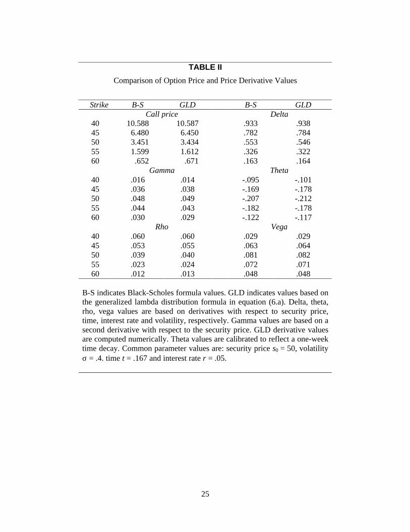
Table II reports option price and price derivative values based on the Black-Scholes
formula and the GLD call price formulas in equation (6.a), with appropriately matched mean,
variance, skewness and kurtosis values. All formulas share common parameter values for the
security price s0 = 50, volatility σ = .4, time t = .167 and interest rate r = .05.
Table II reveals that call price formulas derived from the generalized lambda distribution
yield option price and price derivative values that differ from corresponding Black-Scholes
formula values by at most a few cents. These deviations are similar in magnitude to what is
obtainable using a binomial tree approximation of the Black-Scholes formula (Cox and
Rubinstein (1985), Breen (1991)) and small relative to the price ticks of exchange traded options.

10
RECOVERING A PROBABILITY DISTRIBUTION IMPLIED BY OPTION PRICES
Option pricing formulas based on the generalized lambda distribution (GLD) adapt well to the
problem of recovering a probability distribution from observed option prices. The effectiveness
of such a recovery procedure is demonstrated here and compared with several alternative
procedures using the options price data listed in Table I. For these price data, option maturity is
164 days, the interest rate is 9 percent and the dividend-adjusted index level is 349.21.
Fitting a generalized lambda distribution to the call option price data in Table I involves
estimating the three parameters σ, λ3, λ4 by minimizing the sum of squares stated in equation (7)
immediately below. In equation (7), C(kj,σ,λ3,λ4) represents the GLD call price formula from
equation (6.a) with the arguments s0, t and r suppressed. C(kj) denotes an observed call price for
the strike price kj.
min ( ( , , , ) ( )), ,σ λ λ
σ λ λ3 4
3 42C k C kj j
j
−∑ (7)
Minimizing this sum of squares using the GLD call price formula from equation (6.a)
yields the volatility and shape parameters σ = .168, λ3 = -.065042 and λ4 = -.020756. These
estimates for the parameters λ3 and λ4 imply skewness and kurtosis values of -1.58 and 8.55,
respectively.
Table III compares fitted option prices obtained via this least squares procedure with
fitted values obtained by Rubinstein (1994). Rubinstein’s algorithm produces an implied security
price distribution satisfying the restriction that all fitted option prices lie within observed bid-ask
spreads. This algorithm was later abandoned in Jackwerth and Rubinstein (1996), as it did not
yield solutions with some data sets. However, the fitted prices in the third column of Table III
represent a solution for this data set. For the reader’s convenience, strike prices and bid-ask
average prices from Table I are listed again in the first and second columns, respectively, of
Table III.
Table III also presents fitted option prices obtained using a volatility smile technique and
two density expansion models. The volatility smile technique is based on the quadratic
regression equation stated in equation (8) below, in which IV(k) denotes a fitted implied
volatility for an option with strike price k. Using this function adds just two parameters to the

11
Black-Scholes model. Dumas, Fleming and Whaley (1998) demonstrate the effectiveness of this
parsimonious specification in modeling an implied volatility function.
IV k k s k s R( ) . . / . / .= − − =482 212 096 9950 0
2 2b g (8)
Summing coefficients in this regression yields an at-the-money (k = s0) volatility of σ = .173.
The high regression R2 value indicates that the volatility smile fits a parabolic shape quite well.
The fourth column of Table III reports fitted option prices for each strike computed by
substituting fitted volatility values IV(k) from equation (8) into the Black-Scholes formula.
The two density expansion methods are based on equation (9) below, in which CX
represents an expanded formula composed by a Black-Scholes formula price, denoted by CBS,
and skewness and kurtosis adjustment terms derived from the density function a(St) for the
expiration date security price. Coefficients c3 and c4 are measures related to skewness and
kurtosis deviations, respectively, from a normal or lognormal distribution depending on the
expansion employed.
C Cc da K
dS
c d a K
dSX BSt t
= + +3 42
23 4!
( )
!
( )(9)
In the Jarrow and Rudd (1982) model, equation (9) represents an Edgeworth expansion of the
lognormal density. Alternatively, equation (9) can represent an expansion of the normal density
(Rubinstein (1998)). Corrado and Su (1996, 1997a,b) show that both expansions are effective in
flattening empirical volatility smiles implied by S&P 500 index option prices.
Following least squares procedures to simultaneously estimate implied volatilities and
coefficients of skewness and kurtosis, the lognormal expansion model produces an implied
volatility of σ = .161 and skewness and kurtosis values of -1.253 and 3.188, respectively. The
normal expansion model produces an implied volatility of σ = .178 and skewness and kurtosis
values of -1.648 and 4.934, respectively. The fifth and sixth columns of Table III report fitted
call option prices for each strike using the lognormal and normal density expansion models,
respectively.
Beneath each column of fitted option prices in the third through seventh columns of
Table III are reported root mean squared deviations (RMSD) between fitted prices listed in that

12
column and corresponding bid-ask average prices listed in the second column. These root mean
squared deviations of fitted prices from bid-ask average prices represent a goodness of fit
measure. The RMSD obtained from Rubinstein’s fitted prices and the fitted volatility smile are
$.27 and $.25, respectively. RMSDs based on the lognormal and normal density expansion
models are $.19 and $.21, respectively. In comparison, the GLD call price formula in
equation (6.a) produces call prices resulting in a RMSD of $.23. Differences in magnitude
among these RMSDs appear insignificant relative to the average bid-ask spread of $.78 for these
data.
Figure 2 presents probability densities inferred from the Rubinstein data using the three
recovery methods described earlier. In Figure 2, the smooth, but distinguishably bimodal density
is based on an expansion of the lognormal density. The bimodal density shape reported in
Figure 4 of Rubinstein (1994) is similar, though less pronouncedly bimodal. Not shown here, an
expansion of the normal density yields a recovered density shape that is also distinguishably
bimodal, though slightly less so than that produced by the lognormal expansion.
Figure 2 also plots two unimodal densities with nearly identical shapes. These are the
densities associated with the volatility smile in equation (8) and the GLD call price formula in
equation (6.a). Little visible difference exists between these two densities, except that the mode
of the generalized lambda density lies slightly to the left of the mode of the volatility smile
density.
CALIBRATING AN IMPLIED BINOMIAL TREE TO THE GENERALIZED LAMBDA
DISTRIBUTION
An implied binomial tree infers a stochastic process from a security price distribution and is
widely used to calculate prices for options on futures and other American-style options from
non-standard security price distributions. Rubinstein (1994) points out that his proposed implied
binomial tree algorithm can be used with almost any plausible distribution to obtain a discrete time
stochastic process with a valid limiting diffusion process. Construction of an implied binomial tree
begins by assigning to each of its terminal nodes a nodal value and a nodal probability. An
ordered sequence of N nodal values and probabilities uniquely defines an implied tree with N-1

13
steps. This section describes a method to precisely calibrate the nodal values and probabilities of
an implied tree to the generalized lambda percentile function in equation (4).
The method is straightforward. To calibrate an implied binomial tree with N-1 steps
leading to N terminal nodes, first form an ascending sequence of N+1 strike prices from k0 ≡ 0
through kN ≡ ∞. The N intervals kj+1 - kj > 0, j = 0,1,2,..,N–1 need not be equally spaced, but in
practice at least a subset will normally be selected to match observed equally spaced strike
prices. Precise calibration to the generalized lambda percentile function in equation (4) occurs
when European option prices calculated on the tree for each of the first N strikes match exactly
prices calculated using the corresponding GLD option pricing formula. This requires satisfying
the N equalities stated immediately below, in which C(kj,N) denotes a call price calculated on an
implied tree with N terminal nodes and C k j( , , , )σ λ λ3 4 represents a call price calculated from
equation (6.a):
C k C k N j Nj j( , , , ) , , , , ...,σ λ λ3 4 01 2= ∀ =d i –1
The procedure for determining nodal values and probabilities needed to satisfy these equalities is
described immediately below.
Following the notation used earlier, the probability of a security price realization less than
or equal to the strike price kj is denoted by p(kj). The probability of a security price realization in
the interval kj+1 - kj is therefore p(kj+1) - p(kj), where p(kN+1) ≡ 1 and p(k0) = 0. The probability
p(kj+1) - p(kj) is assigned to node j.
In terms of the generalized lambda percentile function in equation (4), expected values of
security price realizations within the interval kj+1 - kj are specified in equation (10):
E s k s ks p dp
p k p kp j j
p k
p k
j j
j
j
< ≤ =−
=++
+z1
1
1
e j d i d id id i
( )(10)
s ee p k p k
p k p k p k p krt
t j j
j j j j
02 3 4
1
11 1
3
11 1
4
11
1
1
1 1
1
2
3 3 4 4+
− −
×−
+−
− − −
+
FHG
IKJ
F
H
GGGGG
I
K
JJJJJ
F
H
GGGGG
I
K
JJJJJ
+
++ +
++ +
σ
λ λ λ λλ λ λ
λ λ
, ( ) ( ) ( ( )) ( ( ))b gd i d i

14
The expected value E s k s kp j j< ≤ +1e j is assigned to node j for j = 0,1,2,..,N–1.
These nodal values E s k s kp j j< ≤ +1e j and probabilities p(kj+1) - p(kj) precisely calibrate
an implied binomial tree to the percentile function in equation (4). This is demonstrated by
summing expected values of all call option payoffs above the jth strike price to yield this call
price equality:.
C k N e E s k s k k p k p k
e E s k s k k p k
e E s p k
C k
jrt
p i i j i ii j
N
rtp j N j j
rtp j
j
,
max , ( )
( , , , )
d i c hd i b g b gc h
e je j d ie jd i
= < ≤ − −
= < ≤ − −
= −
=
−+ +
=
−+
−
∑ 1 1
1
3 4
1
0
σ λ λ
(11)
In particular, the strike k0 = 0 yields the initial security price C(k0,N) = s0.
This calibration method might be implemented with other distributions. The principal
advantage of the generalized lambda distribution is its adaptability to Monte Carlo applications.
It also allows assigning any of a broad range of skewness and kurtosis values, while maintaining
a unimodal, bell-shaped density. This contrasts with density expansion methods that yield a
unimodal density within only a limited range of skewness and kurtosis values (Stuart and Ord
(1987)). For example, Rubinstein (1998) shows that an expansion of the normal density must
limit the absolute value of skewness to less than one to maintain a unimodal form. The next
section provides a multivariate extension of the generalized lambda distribution.
MULTIVARIATE GENERALIZED LAMBDA DISTRIBUTION
This section begins by developing a multivariate version of the generalized lambda distribution
that facilitates stochastic modeling of multiple, correlated security prices. Immediately
subsequent, the multivariate generalized lambda distribution is extended to a multi-index security
returns model.
Bradley and Fleisher (1994) suggest obtaining correlated generalized-lambda variables
via a transformation from normal variables. Their method proceeds by first generating correlated

15
normal variables using a Cholesky decomposition of the correlation matrix R. They then
compute a univariate p-value for each generated normal variable. These univariate p-values are
then transformed into generalized-lambda variables as, for example, described earlier in this
paper. The correlation matrix G represents the resulting correlation structure among these
generalized-lambda variables.
Bradley and Fleisher (1994) point out that the generalized-lambda correlations and
normal correlations composing the matrices G and R, respectively, will differ somewhat.
Obtaining a precise target configuration for the matrix G requires making incremental
adjustments to the off-diagonal elements of R until the resulting correlation structure in G
converges to the target configuration. Bradley and Fleisher suggest a simulation algorithm to
compute the generalized-lambda correlations in G at each adjustment. However, the accuracy of
the algorithm depends on the size of the simulation and therefore may be computationally
burdensome. A direct approach involves computing generalized-lambda correlations via the
following integral, where the left-side expression γ λ λ λ λ13 14 23 24, , ,b g denotes a correlation
between two generalized-lambda variables with the indicated shape parameters:
γ λ λ λ λ λ λ λ λ ρ13 14 23 24 1 13 14 2 23 24 1 2 1 2, , , ; , ; , , ;b g b gc h b gc h b g=−∞
∞
−∞
∞ zz s N z s N z n z z dz dz
In the right-side integrand, s N zb gc h; ,λ λ3 4 is a unit-variance generalized-lambda variable (a la
equation (1)) generated by the normal probability N zb g and shape parameters λ3 and λ4.
n z z1 2, ; ρb g is a bivariate standard normal density with the correlation parameter ρ. The IMSL
Fortran routine TWODAQ performs this numerical integration quickly and efficiently.
The panel immediately below compares target generalized-lambda correlations with the
normal correlations required to obtain them for the four generalized-lambda densities presented
in Figure 1. The first two columns state skewness and kurtosis values for these densities. As
shown, the required normal correlations are somewhat larger in absolute value than the
generalized-lambda correlations they produce.

16
Skewness KurtosisTarget Generalized-Lambda
Correlations
Required Normal
Correlations0 3 γ ρ-1 6 .1 .104-3 30 .3 -.5 .340 -.583-6 2000 .5 -.3 -.1 .793 -.377 -.141
Development of the multivariate generalized lambda system in the context of a multi-
index model proceeds as follows: Equation (12) immediately below defines the security return yj
as a linear function of the security-specific return xj and the N orthogonal index returns and
factor weights fF and βF,j, respectively.2
y x fj j F j FF
N
= +=
∑ β ,1
(12)
Exact expressions for the variance, skewness and kurtosis of the security return yj are
stated as
Var y Var x Var fj j F j FF
N
( ) ( ) ( ),= +=
∑ β 2
1
Skew y Skew x Var x Skew f Var f Var yj j j F j F FF
N
j( ) ( ) ( ) ( ) ( ) / ( )/,
/ /= +FHG
IKJ=
∑3 2 3 3 2
1
3 2β (13)
Kurt y
Kurt x Var x Var x Var f
Kurt f Var f
Var f Var f
Var yj
j j j F j FF
N
F j F FF
N
F j H j F FH F
N
F
N
j( )
( ) ( ) ( ) ( )
( ) ( )
( ) ( )
/ ( )
,
,
, ,
=
+
+
+
F
H
GGGGGGG
I
K
JJJJJJJ
=
=
= +=
−
∑
∑
∑∑
2 2
1
4 2
1
2 2
11
1
2
6
6
β
β
β β
This multivariate system lends itself to modeling the stochastic properties of portfolios.
Portfolio variance, skewness and kurtosis based on the weights wj, j = 1,2,..,P, for a portfolio of
P securities are stated by these expressions:
2 Elton and Gruber (1987) review multi-index models and provide an extensive bibliography.

17
Var w y w Var x Var f wj jj
P
j jj
P
F j F jj
P
F
N
= = ==∑ ∑ ∑∑FHG
IKJ = +
FHG
IKJ1
2
1 1
2
1
( ) ( ) ,β
Skew w y
w Skew x Var x Skew f Var f w
Var w yj j
j
N j j jj
P
F F j F jj
P
F
N
j jj
N=
= ==
=
∑∑ ∑∑
∑
FHG
IKJ =
+FHG
IKJ
FHG
IKJ
1
3 3 2
1
3 2
1
3
1
3 2
1
( ) ( ) ( ) ( )/ /,
/
β
(14)
Kurt w y
w Kurt x Var x w w Var x Var x
w w Var x Var f
w Kurt f Var f
w Var f w
j jj
N
j j jj
P
k j k jk i
P
j
P
j k F kk
P
j FF
N
j
P
j F jj
P
F FF
N
j F jj
P
F j H jj
=
= = +=
−
===
==
= =∑
∑ ∑∑
∑∑∑
∑∑
∑FHG
IKJ =
+
+FHG
IKJ
+FHG
IKJ
+FHG
IKJ
1
4 2
1
2 2
11
1
2
1
2
11
1
4
2
1
1
2
6
3
6
( ) ( ) ( ) ( )
( ) ( )
( ) ( )
( )
,
,
, ,
β
β
β β1
2
11
1
2
1
P
HH F
N
F
N
j jj
N
Var f
Var w y
∑∑∑
∑
FHG
IKJ
F
H
GGGGGGGGGGGG
I
K
JJJJJJJJJJJJFHG
IKJ
= +=
−
=
( )
These portfolio variance, skewness and kurtosis expressions might be used in conjunction with
the GLD option pricing formulas derived earlier to calculate accurate option values for security
market indexes or other security portfolios.
SUMMARY AND CONCLUSION
This paper introduced the generalized lambda distribution as a flexible tool for modeling non-
lognormal security price distributions. Major advantages of the generalized lambda distribution
include: the flexibility to assign almost any combination of skewness and kurtosis values, ease of
random number generation owing to the simple form of its percentile function, and ready
construction of a multivariate distribution in which each marginal distribution may be assigned
unique skewness and kurtosis values. These advantages suggest several financial applications,
including estimation of option-implied state price densities and risk analyses based on Monte

18
Carlo simulations wherein varied distributional assumptions may be applied to portfolios of
primary and derivative securities.
The generalized lambda distribution is readily applied to the problem of recovering an
implied security price distribution from market-observed option prices. An example of such a
recovery procedure revealed that while estimates based on the generalized lambda distribution
are comparable to those obtained using other methods, generalized-lambda estimates ensure a
unimodal, bell-shaped density. Complementing the recovery of an implied distribution, a method
to calibrate exactly an implied binomial tree to a generalized-lambda density was demonstrated.
Finally, a multivariate version of the generalized lambda distribution was developed that
allows an arbitrary correlation structure among generalized-lambda variables. This development
was extended to a multi-index security returns model and skewness and kurtosis expressions for
linear combinations of correlated generalized-lambda variables were provided. This multivariate
system would be particularly useful in Monte Carlo simulations based on multiple correlated
securities where the experimenter wishes to assign arbitrary skewness and kurtosis values to the
target security price distributions.

19
APPENDIX: CLAMPING THE GENERALIZED LAMBDA DISTRIBUTION
In the case of negative shape parameters, i.e., λ3,λ4 < 0, the range of support for the generalized
lambda distribution spans the real line, thereby assigning positive probabilities to negative security
price values. Jackwerth and Rubinstein (1996) impose clamping to force a price density to zero in
regions where a price realization is disallowed. This imposition is readily applied to the generalized
lambda distribution. The resulting security price percentile function that disallows negative price
realizations is this generalization of equation (1).
s ps e
p
e
pp p
p prt t
( )( ) ( ); ,
( )( ) ( )
=−
+−
− − +−
+−
−+
FHG
IKJ
FHGG
IKJJ
+ +0
2 3 4
1
4
1
31 01
1
01
1 0
1
1 0
1
2
3 4
4 3σλ λ
λ λ
λ λ λ λ λb gb g
(A.1)
The scaling function λ λ λ2 3 40( ( ); , )p defined in equation (A.2) below, in which
β p x y,b g denotes the incomplete beta function, correctly realigns the variance of s(p) in
equation (A.1) on s e ert t0
2 2
1c h e jσ − .
λ λ λ λ
λ λ
λ λβ λ λ β λ λ
λ λ
λ λ
2 3 4 32
1
3
1
4
2 1
3
2 1
43 4 0 3 4
0
1 0
1
1 0
1
1 0
2 1
1 0
2 12 1 1 1 1
3 4
3 4
( ( ); , )
( ) ( )
( ) ( ), ,( )
p sign B A
Ap p
Bp p
p
= × −
=−
+−
−+
=−
++
−+
− + + − + +
+ +
+ +
b gb g
b g b g b gd i
(A.2)
The resulting call price formula is this generalization of equation (6.a).
( ) ( )
( )
( ) ( )
3 3
2
4 4
0 1 2
1
1 1
3
1 12
4
2
1 ( ) / 1 (0)
( ) (0) (0) ( )
11
1 (0) ( ) (0) (1 ( )) (1 (0))
1
1 ( ) / 1 (0)
rt
t
Call s G e kG
G p k p
p k p p p k
e
p p k p p k p
G p k p
λ λ
σ
λ λ
λ
λ
λ
−
+ +
+ +
= −
= − −
− + − +− + − − + − − −
− +
= − −
(A.3)

20
Put-call parity yields the corresponding put price formula:
Put e k G s Grt= − − −− 1 12 0 1b g b g (A.4)
In equations (A.3) and (A.4), the scaling parameter is stated simply as λ2 but is taken from
equation (A.2). With p(0) = 0, equations (A.1), (A.3) and (A.4) all collapse to equations (4), (6.a)
and (6.b), respectively, and therefore are preferred as a more general implementation.
An implementation of clamping might also use these generalizations of the coefficients of
skewness and kurtosis from equation (3), in which A and B are defined in equation (A.2) above:
( ) ( )( ) ( ) ( )( )
( ) ( )( )( ) ( )
43
43
3 2 4
3/2 22 2
3 13 1
4 3 (0) 4 33 4
3 4 (0) 3 4
4 14 1
4 3 (0)3 4
3 2 4 6 3
1 (0)1 (0)3 2 1, 1 2 1, 1
3 1 3 1
3 2 1, 1 2 1, 1
1 (0)1 (0)4 3 1, 1
4 1 4 1
p
p
p
C AB A D AC A B ASkewness Kurtosis
B A B A
ppC
ppD
λλ
λλ
β λ λ β λ λλ λ
β λ λ β λ λ
β λ λ βλ λ
++
++
− + − + −= =
− −
−−= − + + + − + +
+ +
− + + − + +
−−= + − + + −
+ +( )( )
( ) ( )( )( ) ( )( )
4 3
4 3 (0) 4 3
3 4 (0) 3 4
3 1, 1
4 3 1, 1 3 1, 1
6 2 1, 2 1 2 1, 2 1
p
p
λ λ
β λ λ β λ λ
β λ λ β λ λ
+ +
− + + − + +
+ + + − + +
It is worth noting that with plausible parameter values, the probability p(0) is typically
trivial. For example, the generalized lambda distribution was applied to fit an implied security
price distribution to the options price data listed in Table 1. Despite the strong negative skewness
exhibited by this fitted distribution, the derived probability of a negative price realization is only
p(0) = 8.4E-5. Extending the maturity from the original 164 days to 365 days, while retaining all
other parameter values, yields the probability p(0) = 9.0E-4.

21
BIBLIOGRAPHY
Ait-Sahalia, Y., Lo, A.W. (1998): “Nonparametric estimation of state-price densities implicit in
financial asset prices.” Journal of Finance, 53: 499-547.
Amin, K.I., Jarrow, R.A. (1992): “Pricing options on risky assets in a stochastic interest rate
economy,” Mathematical Finance, 2: 217-237.
Amin, K.I., Ng, V.K. (1993): “Option valuation with systematic stochastic volatility,” Journal of
Finance, 48: 881-910.
Bailey, W., Stulz, R.M. (1989): “The pricing of stock index options in a general equilibrium
model,” Journal of Financial and Quantitative Analysis, 24: 1-12.
Bachelier, L. (1964): “Theory of speculation,” Trans. A.J. Boness in P. Cootner, ed. The Random
Character of Stock Market Prices, Cambridge: MIT Press. Translated from dissertation
originally published in 1900.
Bakshi, G., Cao, C., Chen, Z.W. (1997): “Empirical performance of alternative option pricing
models,” Journal of Finance, 52: 2003-2049.
Bakshi, G., Cao, C., Chen, Z.W. (2000): “Do Call Prices and the Underlying Stock Always
Move in the Same Direction?”, Review of Financial Studies, Forthcoming.
Bakshi, G., Chen, Z.W. (1997a): “An alternative valuation model for contingent claims,” Journal
of Financial Economics, 44: 123-165.
Bakshi, G., Chen, Z.W. (1997b): “Equilibrium valuation of foreign exchange claims,” Journal of
Finance, 52: 799-826.
Bates, D.S. (1996): “Jumps and stochastic volatility: Exchange rate processes implicit in
Deutschemark options,” Review of Financial Studies, 9: 69-107.
Bergman, Y.Z., Grundy, B.D., Wiener, Z. (1996): “General Properties of Option Prices”, Journal
of Finance, 51: 1573-1610.
Black, F., Scholes, M.S. (1973): “The pricing of options and corporate liabilities,” Journal of
Political Economy, 81: 637-659.
Bookstaber, R.M., McDonald, J.B. (1987): “A general distribution for describing security price
returns,” Journal of Business, 60: 401-424.
Bradley, D.R., Fleisher, C.L. (1994): “Generating multivariate data from nonnormal
distributions: Mihal and Barrett revisited,” Behavior Research Methods, Instruments, &
Computers, 26: 156-166.

22
Breeden, D.T., Litzenberger, R.H. (1978): “Prices of state-contingent claims implicit in options
prices,” Journal of Business, 51: 621-651.
Breen, R. (1991): “The accelerated binomial option pricing model,” Journal of Financial and
Quantitative Analysis, 26: 153-164.
Buchen, P.W., Kelley, M. (1996): “The maximum entropy distribution of an asset inferred from
option prices,” Journal of Financial and Quantitative Analysis, 31: 143-159.
Corrado, C.J., Su, T. (1996): “Skewness and kurtosis in S&P 500 index returns implied by option
prices,” Journal of Financial Research, 19: 175-192.
Corrado, C.J., Su, T. (1997a): “S&P 500 index option tests of Jarrow and Rudd’s approximate
option valuation formula,” Journal of Futures Markets, 16: 611-630.
Corrado, C.J., Su, T. (1997b): “Implied volatility skews and stock index skewness and kurtosis
implied by S&P 500 index option prices,” Journal of Derivatives, 4: 8-19.
Cox, J.C., Ross, S.A. (1976): “The valuation of options for alternative stochastic processes,”
Journal of Financial Economics, 3: 145-166.
Cox, J.C., Rubinstein, M. (1985): Options Markets, Englewood Cliffs, New Jersey: Prentice
Hall.
Derman, E., Kani, I. (1994): “Riding on a smile,” Risk, 7: 32-39.
Dumas, B., Fleming, J., Whaley, R.E. (1998): “Implied volatility functions: Empirical tests,”
Journal of Finance, 53: 2059-2106.
Dupire, B. (1994): “Pricing with a smile,” Risk, 7: 18-20.
Elton, E.J., Gruber, M.J. (1987): Modern Portfolio Theory and Investment Analysis, New York:
John Wiley and Sons.
Harrison, J.M., Kreps, D.M. (1979): “Martingales and arbitrage in multiperiod securities
markets,” Journal of Economic Theory, 20: 381-408.
Heston, S.L. (1993): “A closed form solution for options with stochastic volatility,” Review of
Financial Studies, 6: 327-343.
Hull, J., White, A. (1987): “The pricing of options on assets with stochastic volatilities,” Journal
of Finance, 42: 281-300.
Jackwerth, J.C., Rubinstein, M. (1996): “Recovering probability distributions from option
prices,” Journal of Finance, 51: 1611-1652.

23
Jarrow, R.A., Rudd, A. (1982): “Approximate option valuation for arbitrary stochastic
processes,” Journal of Financial Economics, 10: 347-369.
Merton, R.C. (1973): “The theory of rational warrant pricing,” Bell Journal of Economics and
Management Science, 4: 141-183.
Merton, R.C. (1976): “The impact on option pricing of specification error in the underlying stock
price returns,” Journal of Finance, 31: 333-350.
Ramberg, J.S., Dudewicz, E.J., Tadikamalla, P.R., Mykytka, E.F. (1979): “A probability
distribution and its uses in fitting data,” Technometrics, 21: 201-214.
Rodriguez, R.N. (1977): “A guide to the Burr type XII distributions,” Biometrika, 64: 129-134.
Ross, S.A. (1976): “Options and efficiency,” Quarterly Journal of Economics, 90: 75-89.
Rubinstein, M. (1994): “Implied binomial trees,” Journal of Finance, 49: 771-818.
Rubinstein, M. (1998): “Edgeworth binomial trees,” Journal of Derivatives, 5: 20-27.
Scott, L.O. (1997): “Pricing stock options in a jump-diffusion model with stochastic volatility
and interest rates,” Mathematical Finance, 7: 413-426.
Stein, E.M., Stein, J. (1991): “Stock price distributions with stochastic volatility,” Review of
Financial Studies, 4: 727-752.
Stuart, A., Ord, J.K. (1987): Kendall's Advanced Theory of Statistics, New York: Oxford
University Press.
Stutzer, M. (1996): “A simple nonparametric approach to derivative security valuation,” Journal
of Finance, 51: 1633-1652.
Tadikamalla, P.R. (1980): “A look at the Burr distribution,” International Statistical Review, 48:
337-344.

24
TABLE I
S&P 500 Index Call Options Data
Call option prices Bid-ask price ButterflyStrikes Bid Ask averages prices
0 349.16 349.26 349.210250 109.47 109.71 109.590275 85.66 86.71 86.185300 63.00 64.04 63.520325 42.00 42.75 42.375330 37.97 38.60 38.285 .130335 34.01 34.64 34.325 .050340 30.10 30.73 30.415 .285345 26.45 27.13 26.790 -.030350 22.79 23.48 23.135 .120355 19.32 19.88 19.600 .195360 15.98 16.54 16.260 .520365 13.13 13.75 13.440 .215370 10.52 11.15 10.835 .515375 8.37 9.12 8.745 .370380 6.65 7.40 7.025 -.050385 4.91 5.60 5.255
Strike, bid and ask prices are reproduced from Figure 4 in Rubinstein(1994). A butterfly price represents a long butterfly position created bybuying a call for each of two outer strikes and writing two calls for the innerstrike. Butterfly prices are based on bid-ask price averages and listed only incases where adjacent strikes are $5 apart.
25
TABLE II
Comparison of Option Price and Price Derivative Values
Strike B-S GLD B-S GLDCall price Delta
40 10.588 10.587 .933 .93845 6.480 6.450 .782 .78450 3.451 3.434 .553 .54655 1.599 1.612 .326 .32260 .652 .671 .163 .164
Gamma Theta40 .016 .014 -.095 -.10145 .036 .038 -.169 -.17850 .048 .049 -.207 -.21255 .044 .043 -.182 -.17860 .030 .029 -.122 -.117
Rho Vega40 .060 .060 .029 .02945 .053 .055 .063 .06450 .039 .040 .081 .08255 .023 .024 .072 .07160 .012 .013 .048 .048
B-S indicates Black-Scholes formula values. GLD indicates values based onthe generalized lambda distribution formula in equation (6.a). Delta, theta,rho, vega values are based on derivatives with respect to security price,time, interest rate and volatility, respectively. Gamma values are based on asecond derivative with respect to the security price. GLD derivative valuesare computed numerically. Theta values are calibrated to reflect a one-weektime decay. Common parameter values are: security price s0 = 50, volatilityσ = .4. time t = .167 and interest rate r = .05.

26
TABLE III
S&P 500 Index Observed and Fitted Call Prices
Fitted call option valuesBid-ask Rubin- Volatility Log-
Strikes average stein smile normal Normal GLD
250 109.590 109.71 109.59 109.20 109.11 109.84275 86.185 86.70 86.22 85.83 85.91 86.47300 63.520 63.90 63.53 63.72 63.82 63.69325 42.375 42.09 42.13 42.50 42.46 42.14330 38.285 37.99 38.09 38.36 38.31 38.07335 34.325 34.01 34.17 34.30 34.26 34.11340 30.415 30.16 30.36 30.36 30.32 30.28345 26.790 26.45 26.70 26.56 26.54 26.59350 23.135 22.90 23.20 22.95 22.95 23.07355 19.600 19.55 19.87 19.56 19.59 19.73360 16.260 16.45 16.74 16.43 16.47 16.61365 13.440 13.65 13.84 13.58 13.62 13.73370 10.835 11.15 11.18 11.03 11.06 11.11375 8.745 8.96 8.79 8.79 8.80 8.78380 7.025 7.07 6.69 6.85 6.83 6.75385 5.255 5.45 4.89 5.21 5.15 5.04
RMSD .27 .24 .19 .21 .23
Bid-ask averages are based on bid and ask call option prices reported inFigure 4 of Rubinstein (1994). Fitted call option values in the third columnare reproduced directly from Rubinstein. Fitted values in the fourth throughseventh columns are computed using the volatility smile specified inequation (8), lognormal and normal density expansion formulas representedby equation (9) and the GLD call price formula in equation (6.a). Root meansquared deviations (RMSD) in third through seventh columns are based ondeviations from corresponding bid-ask averages in second column.

0.00
0.10
0.20
0.30
0.40
0.50
0.60
0.70
0.80
0.90
-4 -3 -2 -1 0 1 2 3
Support
Pro
bab
ility
Generalized lambda density functions with unit variances.
Figure 1

0.000
0.005
0.010
0.015
225 275 325 375 425 475
Index Level
Pro
bab
ility
Option implied probability density functions.
Figure 2