The Double Pareto-Lognormal Distribution – A

New Parametric Model for Size Distributions.

William J. Reed∗

Department of Mathematics and Statistics,University of Victoria,

PO Box 3045, Victoria, B.C.,Canada V8W 3P4

(e-mail:reed@math.uvic.ca).and

Murray JorgensenDepartment of StatisticsUniversity of Waikato

Private Bag 3105, HamiltonNew Zealand.

(e-mail:maj@waikato.ac.nz).

July, 2000. Revised January, October, 2003

∗Research supported by NSERC grant OGP 7252 and originated at the Department ofMathematics and Statistics, University of Melbourne, whose support and hospitality are grate-fully acknowledeged.

1

Abstract

A family of probability densities, which has proved useful in mod-elling the size distributions of various phenomena, including incomes andearnings, human settlement sizes, oil-field volumes and particle sizes, is in-troduced. The distribution, named herein as the double Pareto-lognormalor dPlN distribution, arises as that of the state of a geometric Brownianmotion (GBM), with lognormally distributed initial state, after an expo-nentially distributed length of time (or equivalently as the distribution ofthe killed state of such a GBM with constant killing rate). A number ofphenomena can be viewed as resulting from such a process (e.g. incomes,settlement sizes), which explains the good fit. Properties of the distri-bution are derived and estimation methods discussed. The distributionexhibits Paretian (power-law) behaviour in both tails, and when plottedon logarithmic axes, its density exhibits hyperbolic-type behaviour.

Keywords: size distribution; Pareto law; power-law distribution; fattails; EM algorithm; WWW file size; financial returns.

2

1 Introduction.

The purpose of this paper is to describe a new distribution which has proved to

be very useful in modelling the size distributions of various phenomena arising

in a wide range of areas of inquiry. These include economics (distributions of

incomes and earnings); finance (stock price returns); geography (populations

of human settlements); physical sciences (particle sizes) and geology (oil-field

volumes). A glance ahead to the figures in Sec. 5 will indicate how well the

distribution fits such data.

The distribution, which has four parameters, is somewhat similar in form

to the log-hyperbolic distribution (Barndorff-Nielsen, 1977) and like that dis-

tribution exhibits power-law (Paretian) behaviour asymptotically in both tails.

Also like the log-hyperbolic, it can be derived as a mixture of lognormal dis-

tributions. However the form of the mixing is in a sense more natural, arising

from the distribution of the final state of a geometric Brownian motion (GBM),

killed or stopped with a constant killing rate (or equivalently as the state of a

GBM after an exponentially distributed period of evolution)1. This appears to

be the reason behind the excellent fits obtained for much empirical size data.

Also the new distribution is somewhat simpler to handle analytically than the

log-hyperbolic.

In the next two sections the distribution is defined and its properties, and

those of its close relative, the Normal-Laplace distribution, are presented. Es-1Generalized hyperbolic distributions can also arise as killed GBMs, albeit with more

complicated killing rate functions. See Eberlein (2001) for a discussion of the genesis ofhyperbolic distributions by subordination.

3

timation is discusssed in Section 4 and the paper concludes in Section 5 with

some examples illustrating the excellent fit of the model to a variety of different

empirical size distributions.

2 Genesis and definitions.

Consider a geometric Brownian motion (GBM) defined by the Ito stochastic

differential equation

dX = µXdt + σXdw (1)

with initial state X(0) = X0 distributed lognormally, log X0 ∼ N(ν, τ2). After

T time units the state X(T ) will also be distributed lognormally with

log X(T ) ∼ N(ν + (µ− σ2/2)T, τ2 + σ2T ). (2)

Suppose now that the time T at which the process is observed is an exponentially

distributed random variable with densityfT (t) = λe−λt, t > 0 (or equivalently

that the process is ‘killed’ (e.g. Karlin & Taylor, 1981) with constant killing rate

k(X) ≡ λ and the final ‘killed’ state observed). The distribution of the state

X, say, at the time of observation or killing is a mixture of lognormal random

variables (2) with mixing parameter T .

To find the distribution of X it is easiest to work in the logarithmic scale.

Thus let Y = log X (so that Y is the state of an ordinary Brownian motion

after an exponentially distributed time). The distribution of Y can be shown

(see Appendix in Reed, 2003) to be that of the sum of independent random

variables W and Z say, where Z follows an N(ν, τ2) distribution; and W follows

4

a a skewed Laplace distribution (see e.g. Kotz et al., 2001) with probability

density function (pdf)

fW (w) =

{αβ

α+β eβw, for w ≤ 0αβ

α+β e−αw, for w > 0(3)

where α and −β (α, β > 0) are the roots of the characteristic equation

σ2

2z2 + (µ− σ2

2)z − λ = 0. (4)

The distribution of Y can be obtained by the convolution of the Laplace and

normal densities. It is most conveniently expressed in terms of the Mills’ ratio

of the complementary cumulative distribution function (cdf) to the pdf of a

standard normal distribution:

R(z) =Φc(z)φ(z)

.

With some algebra, the pdf of Y can be shown to be

g(y) =αβ

α + βφ

(y − ν

τ

)[R (ατ − (y − ν)/τ) + R (βτ + (y − ν)/τ)] . (5)

We shall refer to this as the Normal-Laplace distribution and write Y ∼ NL(α, β, ν, τ2)

to indicate that Y follows this distribution.

Note that since a Laplace random variable can be expressed as the dif-

ference between two exponentially distributed variates (Kotz et al. 2001), a

NL(α, β, ν, τ2), random variable, Y , can be expressed as

Yd= ν + τZ + E1/α− E2/β (6)

where E1, E2 are independent standard exponential deviates and Z is a standard

normal deviate independent of E1 and E2. This is the easiest way to generate

5

pseudo-random numbers from the NL distribution. The pdf of X is easily found

from (5). It can be expressed in terms of the Mills’ ratio as

f(x) =1x

g(log x) (7)

or alternatively in terms of the cdf and complementary cdf Φ and Φc of N(0, 1),

asf(x) = αβ

α+β

[A(α, ν, τ)x−α−1Φ

(log x−ν−ατ2

τ

)+

xβ−1A(−β, ν, τ)Φc(

log x−ν+βτ2

τ

)] (8)

where

A(θ, ν, τ) = exp(θν + α2τ2/2). (9)

We shall refer to this distribution as the double Pareto-lognormal distribution

and write

X ∼ dP lN(α, β, ν, τ2)

to indicate that a random variable X follows this distribution. Clearly (from

(6)) a dP lN(α, β, ν, τ2) random variable can be represented as

Xd= UV1/V2 (10)

where U, V1 and V2 are independent, with U lognormally distributed (log U ∼

N(ν, τ2)) and with V1 and V2 following Pareto distributions with parameters α

and β respectively i.e. with pdf

f(v) = θv−θ−1, v > 1

with θ = α and θ = β respectively. Alternatively we can write

Xd= UQ, (11)

6

where Q is the ratio of the above Pareto random variables, so that Q has pdf

f(q) =

{αβ

α+β qβ−1, for 0 < q ≤ 1αβ

α+β q−α−1, for q > 1(12)

We shall refer to the distribution (12) as the double Pareto distribution – hence

the name double Pareto lognormal distribution for the distribution of X (since

such a distribution results from the product of independent double Pareto and

lognormal components).

To generate pseudo-random deviates from the dP lN(α, β, ν, τ2) distribution,

one can exponentiate pseudo-random deviates from NL(α, β, ν, τ2) generated

using (6).

3 Some properties.

Since most of the results concerning the dPlN distribution are most easily de-

rived using the Normal-Laplace we present results for that distribution first.

3.1 The Normal-Laplace distribution.

Two special cases of the Normal-Laplace distribution are of interest, correspond-

ing to α = ∞ and β = ∞. In the latter case the NL distribution is that of the

sum of independent normal and exponentially distributed components and ex-

hibits extra normal variation (i.e. has a fatter tail than the normal) only in the

upper tail. The pdf (5) in this case reduces to

g1(y) = αφ

(y − ν

τ

)R (ατ − (y − ν)/τ) (13)

Similarly with α = ∞ the NL distribution is that of the difference between inde-

pendent normal and exponential components, exhibiting extra normal variation

7

only in the lower tail, and its pdf is

g2(y) = αφ

(y − ν

τ

)R (βτ + (y − ν)/τ)) . (14)

We shall refer to these distributions respectively as the right-handed and left-

handed normal-exponential distributions and use the notation Y ∼ NEr(α, ν, τ2)

to indicate that Y has the pdf g1(y); and Y ∼ NEl(β, ν, τ2) when Y has pdf

g2(y).

We now give some properties of the general NL(α, β, ν, τ2) distribution.

• Cumulative distribution function. A closed-form expression for the cdf of

NL(α, β, ν, τ2) can be obtained. It is

G(y) = Φ(

y − ν

τ

)− φ

(y − ν

τ

)βR(ατ − (y − ν)/τ)− αR(βτ + (y − ν)/τ)

α + β

(15)

This expression is useful for calculating cell probabilities when fitting the model

to grouped data.

•Moment generating function (mgf). From the representation (6) it follows that

the mgf of NL(α, β, ν, τ2) is the product of the mgfs of its normal and Laplace

components. Precisely it is

MY (s) =αβ exp(νs + τ2s2/2)

(α− s)(β + s). (16)

•Mean and variance. Expanding the cumulant generating function, KY (s) =

log MY (s), yields

E(Y ) = ν + 1/α− 1/β; var(Y ) = τ2 + 1/α2 + 1/β2 (17)

8

The third and fourth order cumulants are

κ3 = 2/α3 − 2/β3; κ4 = 6/α4 + 6/β4. (18)

• Representation as a mixture. The NL(α, β, ν, τ2) can be represented as a

mixture of mixture of right-handed and left handed normal-exponential distri-

butions:

g(y) =β

α + βg1(y) +

α

α + βg2(y). (19)

where g1 and g2 are the pdfs of NEr(α, ν, τ2) and NEl(β, ν, τ2) respectively.

• Closure under linear transformation. The NL distribution is closed under

linear transformation. Precisely if Y ∼ NL(α, β, ν, τ2) and a and b are any

constants, then aY + b ∼ NL(α/a, β/a, aν + b, a2τ2).

• Infinite divisibility. The NL distribution is infinitely divisible. This follows

from writing its mgf as

MY (s) =

[exp(

ν

ns +

τ2

2ns2)

(α

α− s

)1/n (β

β + s

)1/n]n

for any integer n > 0 and noting that the term in square brackets is the mgf of

a random variable formed as Z +G1−G2, where Z, G1 and G2 are independent

and Z ∼ N( νn , τ2

n ) and G1 and G2 have gamma distributions with parameters

1/n and α and 1/n and β respectively. The infinite divisibility implies that

it is possible to construct a Levy process with increments following the NL

distribution. Such a process could be used to model the logarithmic returns of

financial instruments (stock prices, foreign currency prices etc.) reflecting the

fact that observed logarithmic returns for high frequency data have fatter tails

than those of the normal distribution (see Sec. 5.5).

9

3.2 The double Pareto-lognormal distribution.

Corresponding to right-handed and left-handed normal-exponential distribu-

tions arising as the two limiting cases of the normal-Laplace distribution are

the right-handed and left-handed Pareto-lognormal distributions with pdfs

f1(x) = αx−α−1A(α, ν, τ)Φ(

log x− ν − ατ2

τ

). (20)

and

f2(x) = βxβ−1A(−β, ν, τ)Φc

(log x− ν + βτ2

τ

). (21)

which are the limiting forms (as β → ∞ and α → ∞) of the dP lN(α, β, ν, τ2)

distribution. Colombi (1990) considered the distribution (20), which he called

the Pareto-lognormal, as a model for income distibrutions.

• Representation as a mixture. From (19) it follows that the dP lN(α, β, ν, τ2)

distribution can be represented as a mixture as

f(x) =β

α + βf1(x) +

α

α + βf2(x). (22)

• Cumulative distribution function. The cdf of dPLN(α, β, ν, τ2) can be written

either as F (x) = G(ex) where G is given by (15); or as

F (x) = Φ(

log x−ντ

)− 1

α+β

[βx−αA(α, ν, τ)Φ

(log x−ν−ατ2

τ

)+

αxβA(−β, ν, τ)Φc(

log x−ν+βτ2

τ

)] (23)

• Power-law tail behaviour. The dP lN(α, β, ν, τ2) distribution exhibits power-

law (or Paretian) behaviour in both tails in the sense that

f(x) ∼ k1 x−α−1 (x →∞); f(x) ∼ k2 xβ−1 (x → 0)

10

where k1 = αA(α, ν, τ) and k2 = βA(−β, ν, τ). The cdf F (x) and complemen-

tary cdf S(x) = 1− F (x) also exhibit power-law tail behaviour with

S(x) ∼ A(α, ν, τ) x−α (x →∞); F (x) ∼ A(−β, ν, τ) xβ (x → 0).

The limiting (Pareto-lognormal) distribution (β = ∞) with pdf f1(x) exhibits

only upper-tail power-law behaviour; while the other limiting (Pareto-lognormal)

distribution (α = ∞) with pdf f2(x) exhibits only lower-tail power-law behav-

iour.

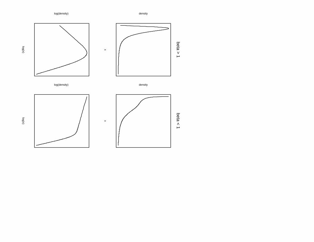
• Shape of distribution. The dP lN(α, β, ν, τ2) pdf is unimodal if β > 1 and

is monotonically decreasing when 0 < β < 1 (see Fig. 1, top row). Like the

log-hyperbolic pdf, when plotted on logarithmic axes, the dP lN(α, β, ν, τ2) pdf

has a shape similar to a hyperbola, with asymptotes of slope −(α+1) and β−1.

In the case 0 < β < 1, both arms have negative slope (see Fig. 1, bottom row).

If the dPlN distribution arises as the final state of a killed GBM, β < 1 if and

only if λ < σ2 − µ.

• Moments. The moment generating function does not exist. However lower-

order moments about zero are easy to obtain. They are

µ′r = E(Xr) =αβ

(α− r)(β + r)exp

(rν + r2τ2/2

)(24)

for r < α. As with the Pareto distribution µ′r does not exist for r ≥ α. The

mean (for α > 1) is

E(X) =αβ

(α− 1)(β + 1)eν+τ2/2 (25)

while the variance and coefficient of variation (for α > 2) are

var(X) =αβe2ν+τ2

(α− 1)2(β + 1)2

[(α− 1)2(β + 1)2

(α− 2)(β + 2)eτ2

− αβ

](26)

11

and

CV =[(α− 1)2(β + 1)2)αβ(α− 2)(β + 2)

eτ2− 1

]1/2

Clearly the CV is independent of ν, increases with τ2 and decreases with α and

β.

• Closure under power-law transformations. The dPlN family of distributions

is closed under power-law transformation. i.e. if X ∼ dP lN(α, β, ν, τ2), then

for constants a, b > 0, W = aXb will also follow a dPlN distribution. Precisely

W = aXb ∼ dP lN(α/b, β/b, bν + log a, b2τ2). (27)

4 Estimation.

4.1 Method of Moments.

Given data assumed to be from the dPlN distribution one could, in principle,

obtain method of moments estimates (MMEs) of α, β, ν and τ2 using the first

four moments of either the dPlN distribution or, having first log-transformed

the data, of the NL distribution. The estimates are not the same. Use of the

dPlN moments (with untransformed data) however is not recommended, since

population moments of order α or greater do not exist. Thus there is in effect

a lower bound (of 4) on the MME of α.

To find MMEs of α and β using the NL distribution, one needs only solve

(18), with κ3 and κ4 set to their sample equivalents. Estimates of ν and τ can

then be obtained from (17). Experience with simulated data has shown that

occasionally (18) has no real solution. This is of no serious consequence since

12

estimates can be obtained by maximum likelihood and we recommend the use of

the method of moments only for finding starting values for iterative procedures

for finding maximum likelihood estimates. In their absence trial and error can

be used.

4.2 Maximum Likelihood.

Unlike MMEs maximum likelihood estimates (MLEs) are the same whether one

fits the dPlN to data x1, x2, . . . , xn or fits the NL to y1 = log x1, . . . , yn = log xn.

The log likelihood function is

` = n log α+n log β−n log(α+β)+n∑

i=1

φ

(yi − ν

τ

)+

n∑i=1

log [R(pi) + R(qi)] (28)

where

pi = ατ − (yi − ν)/τ qi = βτ + (yi − ν)/τ (29)

This can be maximized analytically over ν to yield

ν = y − 1/α + 1/β (30)

and a concentrated (profile) likelihood

ˆ(α, β, τ) = n log α + n log β − n log(α + β) +∑n

i=1 φ(

yi−y+1/α−1/βτ

)+∑n

i=1 log[R(ατ − yi−y+1/α−1/β

τ ) + R(βτ + yi−y+1/α−1/βτ )

].

(31)

This can be maximized numerically using the MMEs as starting values. Note

that it is not difficult to code the score function, nor the elements of the Hessian

matrix for obtaining the observed information matrix.

For grouped data the log-likelihood is of the form

`(α, β, ν, τ2) =N∑

j=1

fj log(G(y(j))−G(y(j−1))) (32)

13

where G is the cdf (15), and −∞ = y(0) < y(1) < . . . , y(N−1) < y(N) = ∞

separate the cells 1, 2, . . . , N .

Both when using grouped and ungrouped data, one can fit either of the limit-

ing (Pareto-lognormal) pdfs f1(x) or f2(x) in a similar fashion, maximizing over

only three parameters. Experience has shown that it is worthwhile examining

the data for evidence of power-law behaviour in the tails. If for example there

is only power-law behaviour in one tail, attempts to fit the dPlN may result in

the non-convergence of the optimization algorithm, while fitting the appropri-

ate Pareto-lognormal pdf (f1 or f2) will be satisfactory. One can examine the

data for power-law tail behaviour, both by plotting (on a logarithmic scale) the

frequencies in a histogram for the logged data; and by plotting the empirical

cdf or complementary cdf on logarithmic axes2. In both cases linearity in the

plots suggests power-law behaviour.

4.3 EM Algorithm.

The representation in Section 2 of a normal-Laplace (NL) variable Y as the

sum of independent random variables W and Z, (where Z follows an N(ν, τ2)

distribution and W follows a a skewed Laplace distribution) suggests that an

approach to ML estimation via the EM algorithm (Dempster, Laird, and Rubin

(1977); McLachlan and Krishnan (1997); Jorgensen (2002)) may prove to be

effective. The EM algorithm uses a likelihood function based on augmented

data as a stepping stone towards the maximization of the likelihood based on2This is equivalent to producing rank-size plots, in which the observations are plotted (on

a logarithmic scale) against their ascending or descending rank (again on logarithmic scale).Zipf’s law, which claims upper-tail power-law behaviour in the size distribution of cities isknown in the urban geography literature as the rank-size property. - see Sec. 5.2.

14

the observed data.

The algorithm alternates between two phases. In the first phase, known as

the E-step, the log-likelihood function based on the augmented data is made to

depend on the original data alone by taking the expectation with respect to the

conditional distribution of the augmented data given the original data. In the

case where the augmented data log-likelihood has exponential family form, the

E-step may be accomplished by taking expectations of the sufficient statistics.

In the M-step an improved set of parameter estimates is constructed so as

to maximize the expected augmented-data log-likelihood. It is shown in the

references given that the new set of parameter estimates cannot have lower

(original data) log-likelihood than the previous set.

Suppose then that we have a sample y1, y2, . . . , yn from the normal-Laplace

distribution. We take the augmented data to be z1, z2, . . . , zn and w1, w2, . . . , wn,

where zi + wi = yi for i = 1, . . . , n, with z1, z2, . . . , zn a sample from N(ν, τ2),

and w1, w2, . . . , wn a sample from the skewed Laplace distribution (3).

The E-step of the can be carried out as follows. Define vi to be 1 if wi ≥ 0,

and 0 otherwise. It is easy to see that the augmented data log-likelihood depends

on the augmented data as a linear function of

zi, z2i , wi, and wivi.

We therefore need to be able to take expectations of quantities of those four

forms with respect to the joint density of (zi, wi) conditional on yi. As zi +wi =

yi we need only the conditional density of wi given yi which more algebra shows

15

to be

h(wi|yi) =τ−1 exp

(tiwi/τ − w2

i /(2τ2))

R(qi) + R(pi)

where

ti = qi(vi − 1)− pivi ={

qi = βτ + yi−ντ if wi < 0

−pi = −ατ + yi−ντ if wi ≥ 0

from which we may obtain

E[wi|yi] = τqiR(qi)− piR(pi)

R(qi) + R(pi)= wi , say

E[wivi|yi] = τ1− piR(pi)

R(qi) + R(pi)= wivi

E[w2i |yi] = τ2 (1 + q2

i )R(qi) + (1 + p2i )R(pi)− τ(α + β)

R(qi) + R(pi).

The conditional expectations of zi and z2i given yi follow easily from these,

completing the E-step.

The M-step may be carried out almost as easily as if we had available

independent random samples z1, z2, . . . , zn from N(ν, τ2) and w1, w2, . . . , wn

from the skewed Laplace distribution with parameters α and β, because in the

augmented-data log-likelihood `c the two distributions are effectively decoupled:

`c = −n log τ − 1τ2

n∑i=1

(zi − ν)2+

n log α + n log β − n log(α + β) + βn∑

i=1

wi(1− vi)− αn∑

i=1

wivi .

Firstly the updated estimates of ν and τ are obtained from conditional expec-

tations of∑

zi and∑

z2i in the usual way. Then define A =

∑i wivi/n and

B = A−∑

i wi/n. The updated estimates of α and β are then

1A +

√AB

and1

B +√

AB

16

respectively. The E-step and the M-step are then repeated until convergence is

reached.

The same caveat regarding whether to fit a dPlN distribution as opposed to

a Pareto-lognormal with power-law behaviour in only one tail (as discussed at

the end of Sec. 4.2) is appropriate here also. If there is power-law behaviour

in only one tail, EM algorithm will be unlikely to converge – it will proceed

making one or other of the parameters α or β progressively larger.

In terms of computing time the EM procedure appears to be more efficient

than the numerical maximization of the 3-parameter concentrated log-likelihood

(Sec. 4.2), probabaly due to the fact that the M-step in the EM procedure is

accomplished analytically. However programming the EM procedure is some-

what more time consuming than simply programming the use of a numerical

optimization routine.

5 Some Applications.

In this section examples of the fit of the dPlN to various size-distribution

datasets are discussed. In two cases the data are grouped (incomes, particle

sizes) while in the others, the actual size observations are available (settlement

sizes, oil-fields, stock price returns). Maximum likelihood estimates of parame-

ters (see Table 1) were obtained under the assumption that the observations

constituted a simple random sample. When the observations do not represent

a true random sample, this method will not of course provide true maximum

likelihood estimates. However it can be justified as providing maximum likeness

17

estimates (Barndorff-Nielsen, 1977) which minimize the discrimination informa-

tion between the fitted distribution and the data.

5.1 Earnings and income distributions.

Examples of the fit of the dPlN (with plots) to various earnings/income distri-

butions are presented in Reed (2003). It was to explain such distributions (and

Pareto’s law of Incomes) that the dPLN (as the state of a killed GBM) was de-

veloped. The explanation revolves around the assumption that an individual’s

earnings (or family’s income) follows GBM (an assumption based on Gibrat’s

law of proportional effects (Gibrat, 1931), common in the income distribution

literature e.g. Champernowne, 1953) and that the population of individuals

(or families) is approximately growing at a fixed rate. Starting incomes are as-

sumed to be lognormally distributed and evolving as GBM. The assumption of

a growing population implies that the time that an individual has been earning

(or a family been in existence) is approximately exponentially distributed, and

thus that current earnings or income follow close to that of a GBM killed with

a constant killing rate.

5.2 Human settlements size.

It has long been recognized that the distribution of size (human population)

of cities within a particular country or jurisdiction frequently exhibits Paretian

behaviour in the upper tail. This phenomenon is known as the rank size property

or in the case when the Pareto exponent is unity as Zipf’s law. There have been

many attempts to explain this phenomenon, two of the more recent being by

18

Gabaix (1999) and Brakman et al. (1999). However the fact that there can also

be Paretian behaviour in the lower tail of the distribution of human settlement

size appears to have escaped notice. Such behaviour in both tails is manifest

in the dPlN distribution which turns out to fit settlement size data very well

(see Reed, 2002, for examples). The good fit can be explained in a similar

way to that of incomes/earning data. If it is assumed that the growth in size

of settlements follows GBM (e.g. Gabaix, 1999), then provided that the time

since foundation follows an exponential distribution, and that at foundation

sizes are lognormally distributed, then the current sizes should follow the dPlN

distribution. The approximate exponential form of the distribution of the time

since foundation follows if the foundation of settlements occur in a Yule process

(Yule, 1924) (i.e. homogeneous pure birth process) over a long time period.

Such an assumption seems reasonable, corresponding to the situation in which

existing settlements create satellites at a fixed probabilistic rate.

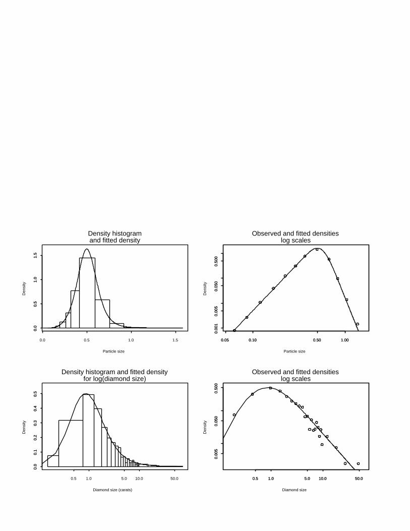
5.3 Particle size.

Fig. 2 shows the fit of the dPlN to grouped data on aeolian sand particle size

and diamond particle size presented in Barndorff-Nielsen (1977) who fitted the

log-hyperbolic distribution to these data. Visual inspection of Fig. 4 and of the

graphs in Barndorff-Nielsen (1977) suggest very similar fits for the two models.

It may be possible to view the size of a particle as the outcome of a killed

multiplicative (geometric) stochastic process (i.e. as the result of a random

number of random fractures), although perhaps not precisely as the result of

GBM with a constant killing rate. In spite of the fact of no explanatory model

19

for why particle sizes should exactly follow dPlN, the empirical fit is nonetheless

extremely good.

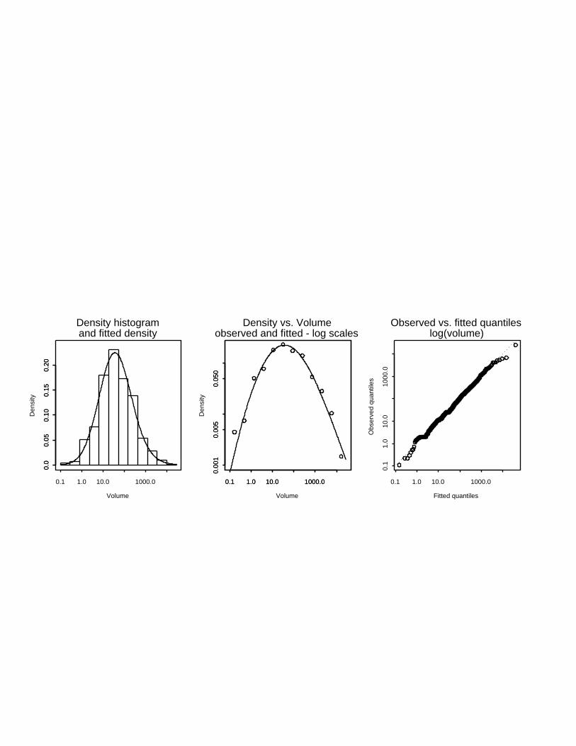
5.4 Oil-field size.

Fig. 3 shows the dPlN distribution fitted to the volumes of 634 oil fields in the

West Siberian Basin3 (the world’s largest oil province). The fit is very good

except possibly in the extreme upper tail. An oil-field can be thought of as a

percolation cluster (Stauffer and Aharony, 1992) and thus as a killed stochastic

process, although not of course exactly as a killed GBM.

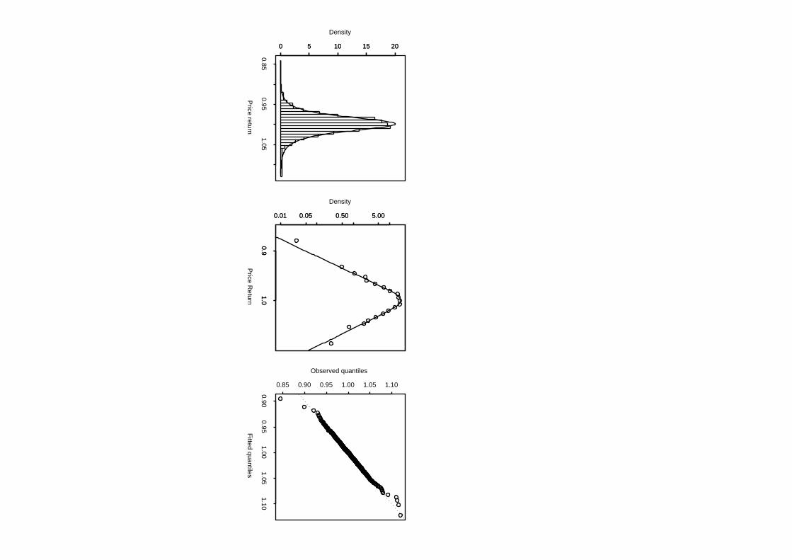
5.5 Stock price returns.

It has been recognized for some time (see e.g Rydberg, 2000 for a discussion)

that the logarithmic returns log[P (t + 1)/P (t)], of a stock whose price Pt is

observed at discrete times t = 1, 2, . . . follow a distibution with fatter tails than

that of the normal distribution predicted by the standard GBM model of stock

price movement. Furthermore the departures from normality increase as the

reporting interval shortens. Various alternatives have been proposed including

the asymmetric Laplace distribution (e.g. Madan and Milne, 1991; Kozubowski

and Podgorski, 2001); and the generalized hyperbolic (Eberlein, 2001). For both

of these alternatives option pricing formulas (a la Black-Scholes) have been de-

veloped. The crucial fact that enables this is that in both cases the distributions

are infinitely divisible, so that a Levy process can be constructed for which the

increments (representing logarithmic returns) have the given distribution.

3Data from http://energy.cr.usgs.gov:8080/energy/WorldEnergy/OF97-463 a website ofU.S Dept. of Interior Geological Survey.

20

The dPlN distribution is similar in form to the log-hyperbolic (and the NL

similar to the hyperbolic) and provides another candidate for stock-price re-

turns. Fig 4 shows the fit of the NL to the logarithmic daily returns using the

closing price of IBM ordinary stock from Jan 1, 1999 to Sept. 18, 2003 (929

observations). The NL distribution is infinitely divisible and so it possible to

construct a Levy process for the movement of stock prices, based on this distri-

bution. Option prices for this model can be evaluated using the characteristic

function approach (e.g. Schoutens, 2003, p. 20).

5.6 Size of WWW sites and computer files – a potentialapplication.

Huberman and Adamic (1999) have shown that the size distribution (number of

pages) of World-Wide Web sites follows power-law behaviour in the upper-tail,

while Mitzenmacher (2001) showed that both upper- and lower-tail power-law

behaviour occurs in the distribution of file sizes. Both papers offerred an expla-

nation analogous to the derivation of the double Pareto distribution described

in Sec. 2, viz. that it results from a multiplicative process observed after a

geometrically distributed number of steps. No attempt is made to fit a theo-

retical distribution to the data, in either paper. However Mitzenmacher points

out that file size distributions ‘have a lognormal body and Pareto tail’. This

suggests the dPlN as an obvious candidate for such data.

21

REFERENCES

Barndorff-Nielsen, O. Exponentially decreasing distributions for the logarithm

of particle size. Proc. R. Soc. Lond. A. 1977, 353, 401-419

Brakman, S., H. Garretsen, C. Van Marrewijk and M. van den Berg (1999) The

return of Zipf: towards a further understanding of the rank-size distribution, J.

Reg. Sci,, 1999, 29, 183-213.

Colombi, R. A new model of income distribution: ThePareto lognormal distri-

bution. In Income and wealth distribution, inequality and poverty, C. Dagum

and M. Zenga, (eds.), Springer, Berlin, 1990.

Champernowne, D. A model of income distribution, Econ. J., 1953, 63, 318-

351.

Dempster, A.P., Laird, N.M., D. B. Rubin. Maximum likelihood from incom-

plete data via the EM algorithm, J. Roy. Stat. Soc. 1977, B39, 1-38.

Eberlein E. Applications of generalized hyperbolic Levy motions to finance.

Levy Processes: Theory and Applications. O. Barndorff-Nielsen, T. Mikorsky

and S. Resnick (eds.). Birkhauser, Boston, 2001.

Gabaix, X. Zipf’s Law for cities: an explanation, Quart. J. Econ., 1999, 114,

739-767.

Gibrat, R.Les inegalites economiques, Librairie du Recueil Sirey, Paris, 1931.

Huberman, B. and L. A. Adamic. Internet: Growth dynamics of the World-

Wide web. Nature, 1999, 401, 130-131.

22

Jorgensen, M. Expectation-maximization algorithm, Encyclopedia of Environ-

metrics, A. H. El-Shaarawi and W. W. Piegorsch (eds). J. Wiley and Sons, New

York, 2001.

Karlin, S. and H. M. Taylor. An Introduction to Stochastic Processes, Vol II,

New York, Academic Press, 1981.

Kotz, S., T. J. Kozubowski and K. Podgorski. The Laplace Distribution and

Generalizations. Birkhauser, Boston, 2001.

T. J. Kozubowski and K. Podgorski. Asymmetric Laplace laws and modeling

financial data, Math. Comput. Model., 2001, 34, 1003-1021.

Madan, D.B.and F. Milne. Option pricing with VG martingale components.

Math. Fin., 1991, 1 39-55.

McLachlan, G.J. and T. Krishnan. The EM algorithm and Extensions. J. Wiley

and Sons, New York, 1997.

Mitzenmacher, M. Dynamic models for file sizes and double Pareto distributions.

2001, Draft manuscript avilable at

http://www.eecs.harvard.edu/ michaelm/NEWWORK/papers/.

Reed, W. J. The Pareto law of incomes - an explanation and an extension.

Physica A, 2003, 319, 579-597.

Reed, W. J. On the rank-size distribution for human settlements. J. Reg. Sci.,

2002, 42 1-17.

Rydberg, T. H. (2000). Realistic statistical modelling of financial data. Inter.

Stat. Rev., 2000, 68, 233-258.

23

Schoutens, W. Levy Processes in Finance, J. Wiley and Sons, Chichester, 2003.

Stauffer, D and A. Aharony (1992). Introduction to Percolation Theory, London,

Taylor and Francis, 1992.

Yule, G., (1924) A mathematical theory of evolution based on the conclusions

of Dr. J. C. Willis, F.R.S., Philos. Trans. B, Roy. Soc. London, 1924, 213

21-87.

24

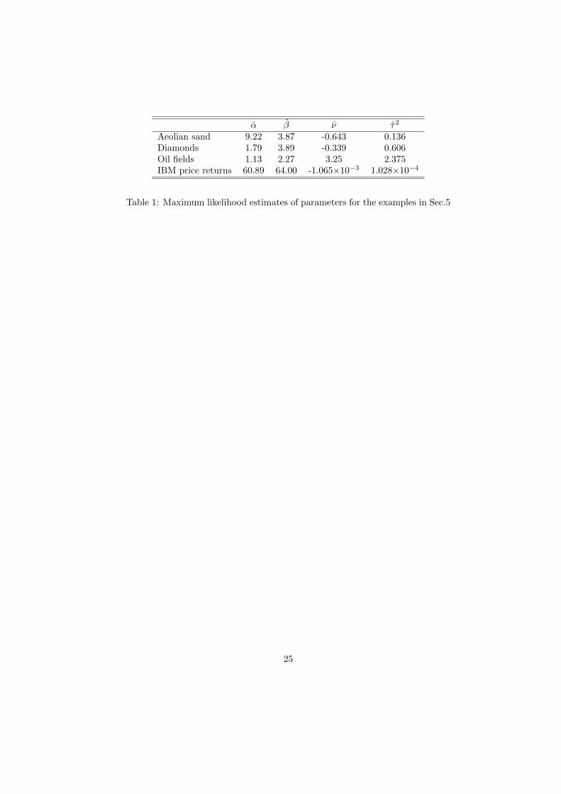
α β ν τ2

Aeolian sand 9.22 3.87 -0.643 0.136Diamonds 1.79 3.89 -0.339 0.606Oil fields 1.13 2.27 3.25 2.375IBM price returns 60.89 64.00 -1.065×10−3 1.028×10−4

Table 1: Maximum likelihood estimates of parameters for the examples in Sec.5

25

Figure captions.

Fig.1 Two forms of the double Pareto-lognormal density, in the natural scale (top

row) and logarithmic scales (bottom row). The panels in the left-hand column show

the case β > 1 and those in the right-hand column the case β < 1.

Fig.2 Empirical and fitted dPlN distributions for aeolian sand particle size in millime-

tres (top row) and diamond size in carats from a South West African diamond mine

(bottom row) using data in Barndorff-Nielsen (1977). In each case the left-hand panel

shows a density histogram and the dPlN fitted density (size in logarithmic scale) while

the right-hand panels shows the empirical density (calculated from histogram) and the

fitted dPlN density (density and size both in logarithmic scales).

Fig.3 Empirical and fitted dPlN distributions for the volume (mmb) of 634 oil fields in

the West Siberian basin. The left-hand panel shows a density histogram and the fitted

dPlN density (volume in logarithmic scale). The centre panel shows the empirical

density (calculated from histogram) and fitted dPlN distribution (density and volume

both on logarithmic scales) and the right-hand panel shows a quantile-quantile plot of

the empirical and fitted dPlN distributions (both in logarithmic scales).

Fig.4 Empirical and fitted dPlN distributions for the daily price returns on IBM

common stock. The left-hand panel shows a density histogram and the fitted dPlN

density. The centre panel shows the empirical density (calculated from histogram)

and fitted dPlN distribution (density and price return both on logarithmic scales) and

the right-hand panel shows a quantile-quantile plot of the empirical and fitted dPlN

distributions.

26

x

density

beta > 1

x

density

beta < 1

log(x)

log(density)

log(x)

log(density)

0.0

0.5

1.0

1.5

Particle size

Den

sity

0.0 0.5 1.0 1.5

0.0

0.5

1.0

1.5

Density histogramand fitted density

0.05 0.10 0.50 1.00

0.00

10.

005

0.05

00.

500

Particle size

Den

sity

0.05 0.10 0.50 1.00

0.00

10.

005

0.05

00.

500

Observed and fitted densitieslog scales

0.0

0.1

0.2

0.3

0.4

0.5

Diamond size (carats)

Den

sity

0.5 1.0 5.0 10.0 50.0

0.0

0.1

0.2

0.3

0.4

0.5

Density histogram and fitted densityfor log(diamond size)

0.5 1.0 5.0 10.0 50.0

0.00

50.

050

0.50

0

Diamond size

Den

sity

0.5 1.0 5.0 10.0 50.0

0.00

50.

050

0.50

0

Observed and fitted densitieslog scales

0.0

0.05

0.10

0.15

0.20

Volume

Den

sity

0.1 1.0 10.0 1000.0

0.0

0.05

0.10

0.15

0.20

Density histogramand fitted density

0.1 1.0 10.0 1000.0

0.00

10.

005

0.05

0

Volume

Den

sity

0.1 1.0 10.0 1000.0

0.00

10.

005

0.05

0

Density vs. Volumeobserved and fitted - log scales

Fitted quantiles

Obs

erve

d qu

antil

es

0.1 1.0 10.0 1000.0

0.1

1.0

10.0

1000

.0

Observed vs. fitted quantileslog(volume)

0 5 10 15 20

Price return

Density

0.850.95

1.05

0 5 10 15 20

Price R

eturn

Density

0.91.0

0.01 0.05 0.50 5.00

0.91.0

0.01 0.05 0.50 5.00

Fitted quantiles

Observed quantiles

0.900.95

1.001.05

1.10

0.85 0.90 0.95 1.00 1.05 1.10