Review of Lognormal Statistics andReview of Lognormal Statistics and analyzing small data sets

Review of IH StatisticsI. Lognormal distributiongII. Sample 95th percentileIII. UCL for the sample 95th percentileIV. Rules-of-thumb for “Eyeballing” Exposure Data

2

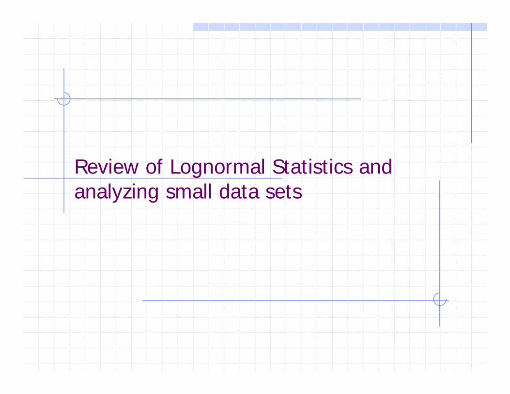
I. Lognormal Distribution – Exampleg pAirborne exposures to inorganic lead

3

source: Cope et al. AIHAJ 40:372-379, 1979

Copyright 2007 Exposure Assessment Solutions, Inc. 4

Parameters vs. StatisticsParameters Statistics

-calculated using all elements of the population-log transform each element

-calculated from a sample of n elements randomly selected-log transform each element-log transform each element -log transform each element

Population Mean

μSample Mean

y_μ y

Population Standard Deviation

Sample Standard Deviation

y

Standard Deviation σ Deviation sy y

Th t t d t t l l l ( )

5

The measurements are converted to natural logs: y = ln(x)

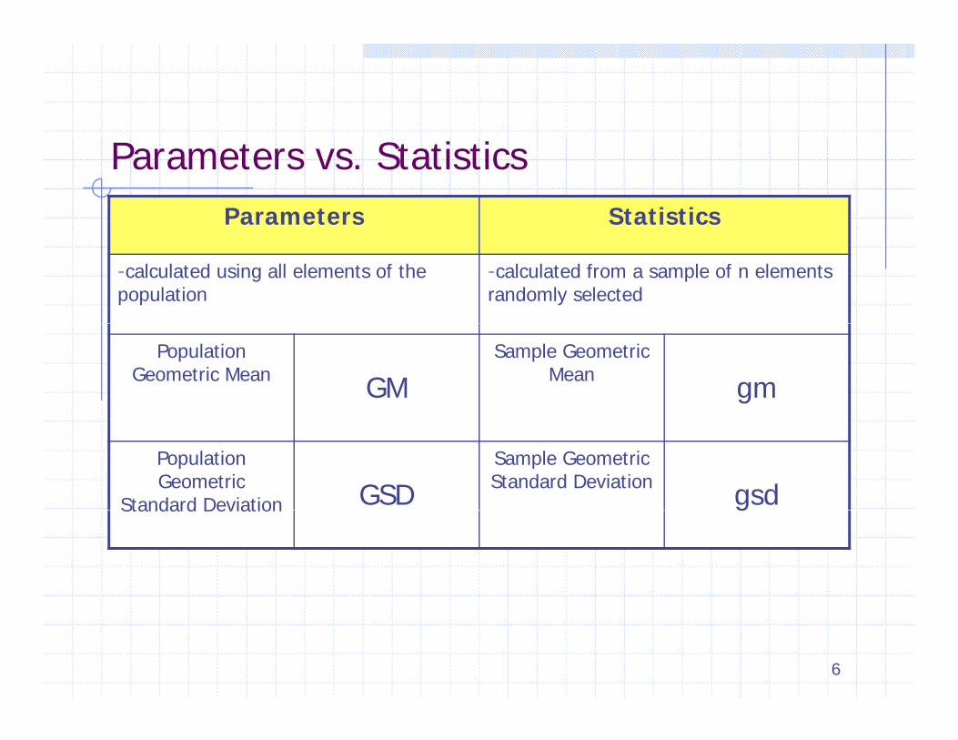
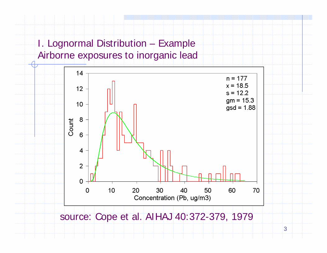
Parameters vs. StatisticsParameters Statistics

-calculated using all elements of the population

-calculated from a sample of n elements randomly selected

Population Geometric Mean GM

Sample Geometric Mean gm

Population Geometric

Standard Deviation GSDSample Geometric Standard Deviation gsdStandard Deviation g

6

Lognormal distribution PDF

GM

7

Lognormal

8

Sample geometric mean (gm) &p g (g )geometric standard deviation (gsd)

9

Example: Welding fume data -estimate GM and GSD

Case xi (mg/m3) yi=ln(xi) (yi-y)2

1 0.84 -0.1744 0.055877

2 0 98 -0 0202 0 006762

_

2 0.98 -0.0202 0.006762

3 0.42 -0.8675 0.864025

4 1.16 0.1484 0.007463

5 1.36 0.3075 0.060248

6 2.66 0.9783 0.839600

Sum = 0.3722 1.833976

y = 0.0620

gm = 1 06

_

10

gm = 1.06

gsd = 1.83

Example: Welding fume data -estimate GM and GSD

11

Example: Welding fume data -estimate μ and σ

Case xi (mg/m3) ( xi-x )2

1 0.84 0.157344

_

2 0.98 0.065878

3 0.42 0.666944

1 164 1.16 0.005878

5 1.36 0.015211

6 2 66 2 0258786 2.66 2.025878

Sum = 7.42 2.937133

1 24_

12

x = 1.24

sd = 0.77

Example: Welding fume data -estimate μ and σ

13

14

1.2 3.1

GSD = X84/X50 = 3 1/1 2 = 2 6GSD X84/X50 3.1/1.2 2.6

II. Sample 95th Percentile ExposureThe focus is on the upper tail of the exposure profile.The sample 95th percentile can be considered a “decision statistic”. The (usual) goal is to determine which category the 95th

P til t lik l f llPercentile most likely falls.It is used to assist in reaching a decision that the exposure profile is

“Controlled” or “Acceptable”Controlled or Acceptable“Unacceptable”or falls in a “Control Category”

16

95th Percentile interpretation of TWA OELs

ACGIHRoach, S.A., Baier, E.J., Ayer, H.E., and Harris, R.L.: Testing compliance with Threshold Limit Values for respirable dusts. American Industrial Hygiene Association Journal 28:543-553 (1967).Stokinger, H.E.: Industrial air standards - theory and practice. Journal ofStokinger, H.E.: Industrial air standards theory and practice. Journal of Occupational Medicine 15:429-431 (1973).Still, K.R. and Wells, B.: Quantitative Industrial Hygiene Programs: Workplace Monitoring. (Industrial Hygiene Program Management series, part VIII) Applied Industrial Hygiene 4:F14-F17 (1989)part VIII). Applied Industrial Hygiene 4:F14-F17 (1989).

17

95th Percentile interpretation of TWA OELs

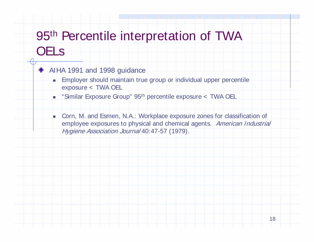
AIHA 1991 and 1998 guidanceEmployer should maintain true group or individual upper percentile exposure < TWA OEL“Similar Exposure Group” 95th percentile exposure < TWA OEL

Corn, M. and Esmen, N.A.: Workplace exposure zones for classification of employee exposures to physical and chemical agents. American Industrial Hygiene Association Journal 40:47-57 (1979).

18

95th Percentile interpretation of TWA OELs

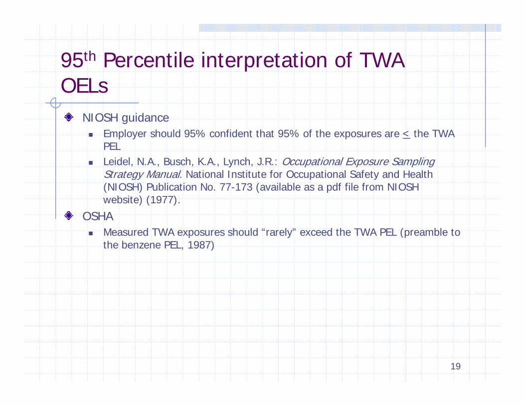
NIOSH guidanceEmployer should 95% confident that 95% of the exposures are < the TWA PELLeidel, N.A., Busch, K.A., Lynch, J.R.: Occupational Exposure Sampling Strategy Manual. National Institute for Occupational Safety and HealthStrategy Manual. National Institute for Occupational Safety and Health (NIOSH) Publication No. 77-173 (available as a pdf file from NIOSH website) (1977).

OSHAM d TWA h ld “ l ” d h TWA PEL ( blMeasured TWA exposures should “rarely” exceed the TWA PEL (preamble to the benzene PEL, 1987)

19

95th Percentile interpretation of TWA OELs

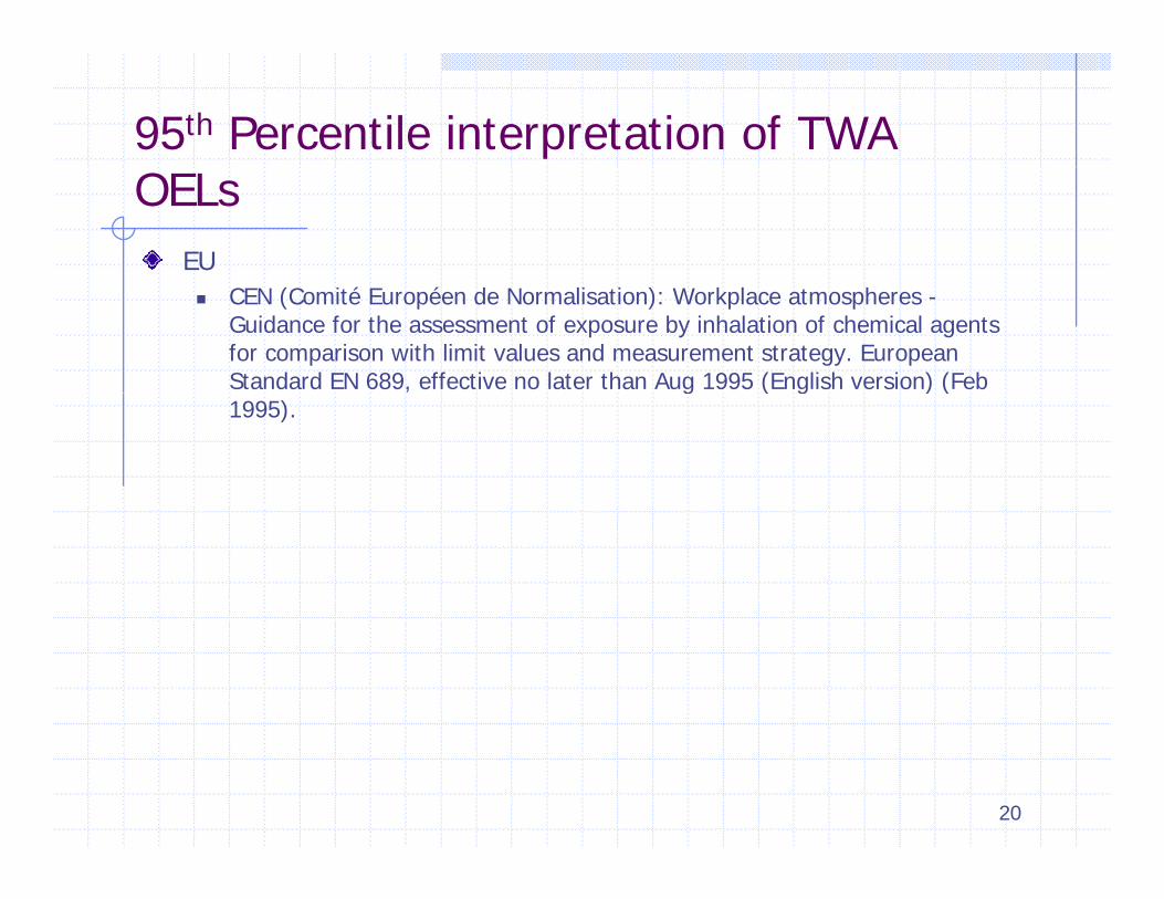
EUCEN (Comité Européen de Normalisation): Workplace atmospheres -Guidance for the assessment of exposure by inhalation of chemical agents for comparison with limit values and measurement strategy. European Standard EN 689, effective no later than Aug 1995 (English version) (Feb , g ( g ) (1995).

20

ExampleA sample of six full-shift TWA welding fume p gmeasurements resulted in the following statistics:

(sample) geometric mean is 1.06 mg/m3

(sample) geometric standard deviation is 1 83(sample) geometric standard deviation is 1.83

What is the point estimate (i.e., best estimate) of the true 95th percentile?

21

90th, 95th, and 99th Percentiles

22

95th Percentile

23

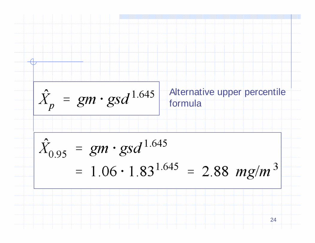
Alternative upper percentileformulaformula

24

Focus on Upper Tail

25

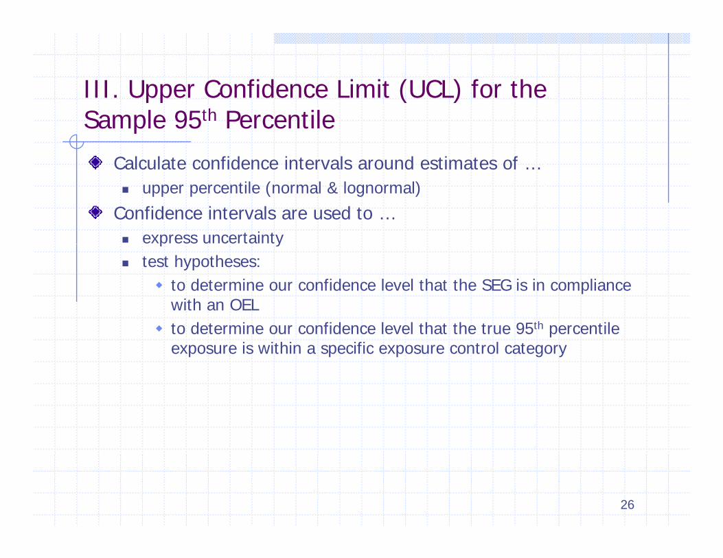
III. Upper Confidence Limit (UCL) for the Sample 95th Percentile

Calculate confidence intervals around estimates of …upper percentile (normal & lognormal)

Confidence intervals are used to …express uncertaintyp ytest hypotheses:

to determine our confidence level that the SEG is in compliance with an OELto determine our confidence level that the true 95th percentile exposure is within a specific exposure control category

26

For single shift, TWA exposure limits (TWA OELs) …g , p ( )focus on the upper tail of the distributione.g., 95th percentile exposure

27

Upper Percentile (e.g., 95th percentile)Concept

Calculate the 95% upper confidence interval for the 95th percentile statistic (upper tolerance limit)

Application95%UCL can be used to test the following hypotheses:95%UCL can be used to test the following hypotheses:

Ho: 95th percentile > OELHa: 95th percentile < OEL

I t t tiInterpretationIf the 95%UCL is less than the OEL, then we can say that we are at least 95% confident that the true 95th percentile is less than the OEL

28

95%UCL for the 95th PercentileProcedure:

Calculate the gm and gsdUsing n, read the UCL K-value from the appropriate table

γ = confidence level, e.g., 0.95γp = proportion, e.g., 0.95n = sample size

Using gm, gsd, and k, calculate the 95%UCLg g , g , ,y = ln( gm )sy = ln( gsd )

_

29

30

31

32

IV. Rule-of-thumb for “Eyeballing” Exposure Data

Given:G = medianXp = G x DZp (e.g., X0.95=G x D1.645)

R l f th b id li b d i d f… a Rule-of-thumb, or guideline, can be devised for quickly estimating from limited data the range in which the true 95th percentile might lie.

33

Multiple of GM (median)

GSD Xp = 95th percentile

Zp = 1.645

1.5 1.95

2.0 3.13

2.5 4.51

3.0 6.09

34

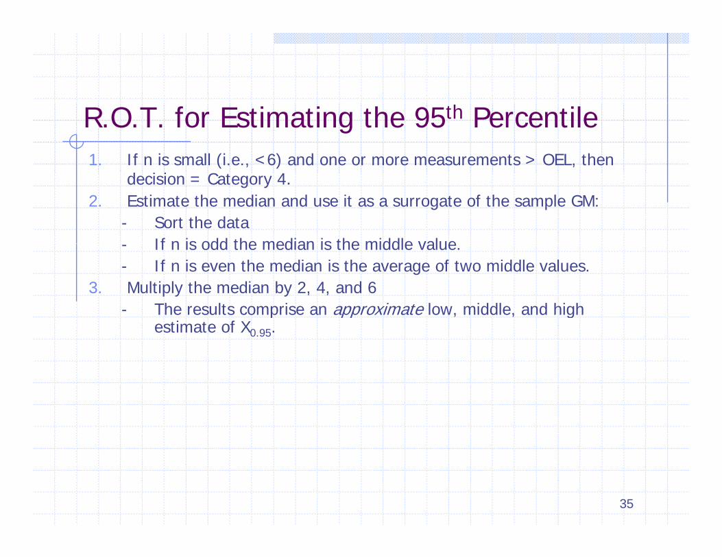
R.O.T. for Estimating the 95th Percentile1. If n is small (i.e., <6) and one or more measurements > OEL, then

d i i C t 4decision = Category 4.2. Estimate the median and use it as a surrogate of the sample GM:

- Sort the dataIf n is odd the median is the middle value- If n is odd the median is the middle value.

- If n is even the median is the average of two middle values.3. Multiply the median by 2, 4, and 6

- The results comprise an approximate low, middle, and highThe results comprise an approximate low, middle, and high estimate of X0.95.

35

Rule-of-thumb Workshop(assume OEL=100)a. X = {5}bb. X = {68}c. X = {7, 34, 57}d. X = {1, 1, 2, 5}e X {4 5 8 23}e. X = {4, 5, 8, 23}f. X = {0.3, 1, 2, 3, 4, 22}g. X = {10, 10, 10, 20, 50, 105}h X = {7 10 16 21 45 53}h. X = {7, 10, 16, 21, 45, 53}

For each dataset, determine the appropriate Exposure Category – 1, 2, 3, or 4 – using the above Rule-of-thumb.

36

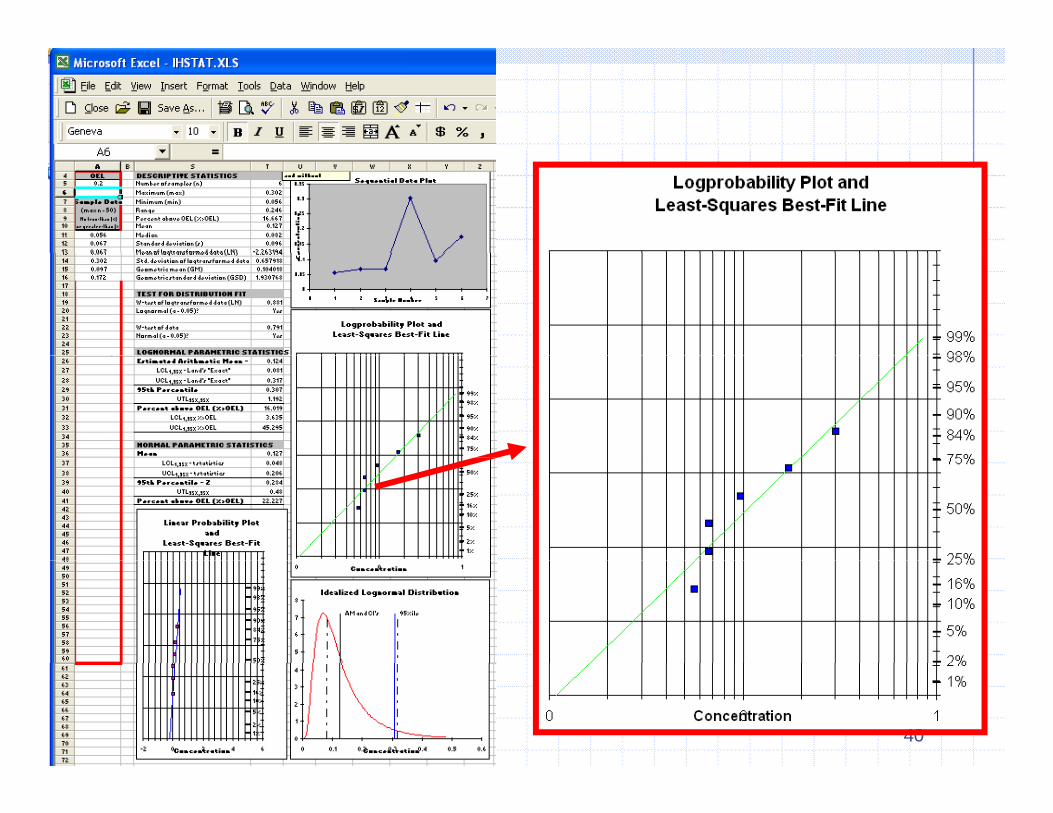
Available Data Analysis ToolsIHStats.xls

Comes with the AIHA 3rd Edition “Exposure Assessment and Management …”handles n<50handles n<50

EASC-IHStats.xlswww.aiha.org/1documents/committees/EASC-IHSTAT.xls An update of the IHStats.xls spreadsheethandles n<200multiple languagesmultiple languages

37

38

39

40

41

42

43

44

45