HERA, 96-26

Using Lognormal Distributions and Lognormal Probability Plotsin Probabilistic Risk Assessments

David E. BurmasterDelores A. Hull

Alceon CorporationPO Box 382669Cambridge, MA 02238-2669

tel: 617-864-4300fax: 617-864-9954email: deb@Alceon.com

Running Head: Using Lognormal Distributions in Risk Assessments

Contents:

• Abstract

• Key Words

• Introduction to Lognormal Distributions

• Concepts and Notations for Random Variables

• Symbolic Approach

• The Two-Parameter Lognormal Distribution

• Percentiles of Random Variables ln[X] and X

• Arithmetic Central Moments of Random Variables ln[X] and X

• Geometric Moments of Random Variable X

• Different Ways to Parameterize the Lognormal Distribution

• A Constant Times a Lognormal Distribution

• Products and Quotients of Lognormal Distributions

• A Simplified Way to Fit Lognormal Distributions to Data

• Discussion of the Simplified 8-Step Method

• Numerical Simulations with Lognormal Variables

• Introduction to Lognormal Probability Plots

• The Functions p(z) and z(p)

• Computing the Function z(p)

• Plotting a Lognormal Probability Plot

• Discussion of Lognormal Probability Plots

• End Notes

• Dedication and Acknowledgement

• References

1

HERA, 96-26

Abstract

Lognormal distributions play a central role in human and ecological risk assessment, so

every risk assessor needs to understand and exploit their basic properties. Similarly,

Lognormal probability plots are invaluable because they provide a powerful way to

visualize measured data or simulated results.

Key Words

Lognormal distribution, Lognormal probability plot

3

HERA, 96-26

Introduction to Lognormal Distributions

Lognormal distributions (with two parameters) have a central role in human and

ecological risk assessment for at least three reasons. First, many physical, chemical,

biological, toxicological, and statistical processes tend to create random variables that

follow Lognormal distributions (Hattis and Burmaster, 1994). For example, the physical

dilution of one material (say, a miscible or soluble contaminant) into another material

(say, surface water in a bay) tends to create non equilibrium concentrations which are

Lognormal in character (Ott, 1995; Ott, 1990). Second, when the conditions of the

Central Limit Theorem obtain (Mood, Graybill, and Boes, 1974), the mathematical

process of multiplying a series of random variables will produce a new random variable

(the product) which tends (in the limit) to be Lognormal in character, regardless of the

distributions from which the input variables arise (Benjamin and Cornell, 1970). Finally,

Lognormal distributions are self-replicating under multiplication and division, i.e.,

products and quotients of Lognormal random variables are themselves Lognormal

distributions (Crow and Shimizu, 1988; Aitchison and Brown, 1957), a result often

exploited in back-of-the-envelope calculations.

Concepts and Notations for Random Variables

In this review, we use the symbol V to denote a positive random variable, i.e., a variable

in an equation that can take any value greater than zero. Here, the underscore indicates

that V is a random variable. The relative frequency of values sampled (or "realized")

from the distribution is governed by a mathematical function called a probability

distribution (Freund, 1971). We use random variables described by probability

4

HERA, 96-26

distributions to represent the variability inherent in a quantity (Morgan and Henrion,

1990).

Symbolic Approach

In this presentation, we do not manipulate the probability density function (PDF) or the

cumulative distribution function (CDF) for any distributions (Feller, 1968; Feller, 1971;

Stuart and Ord, 1987; Stuart and Ord, 1991). Instead, we demonstrate an alternative

symbolism, complete with its own algebra, that makes the concepts and the calculations

easier to understand (Springer, 1979). This abstract symbolism is, of course, not what a

computer does in a numerical simulation with Monte Carlo or Latin Hypercube sampling.

Computer algorithms are beyond the scope of this review (Morgan, 1984; Knuth, 1981;

Rubinstein, 1981). In this symbolic notation, one writes the sentence "the random

variable V is distributed as a Normal distribution" as follows: V ~ Normal(parameters).

The Two-Parameter Lognormal Distribution

The 2-parameter Lognormal distribution takes its name from the fundamental property

that the logarithm of the random variable is distributed according to a Normal or

Gaussian distribution (Evans, Hastings, and Peacock, 1993; Crow and Shimizu, 1988;

Aitchison and Brown, 1957):

ln[X] ~ N(µ, σ) Eqn 1

where ln[•] denotes the natural or Napierian logarithm function (base e) and N(•, •)

denotes a Normal or Gaussian distribution with two parameters, the mean µ and the

standard deviation σ (with σ > 0). In Eqn 1, X is a Lognormal random variable, and ln[X]

5

HERA, 96-26

is a Normal random variable. By convention, X is called a Lognormal random variable

because its logarithm follows a Normal distribution. In Eqn 1, µ is the mean and σ is the

standard deviation of the distribution for the Normal random variable ln[X], not the

Lognormal random variable X. Although sometimes confusing, µ is also the median of

the Normal random variable ln[X] because µ is the median of N(µ, σ). Eqn 1 represents

the Lognormal random variable X in "logarithmic space." As can be seen in Eqn 1, the

random variable ln[X] follows a Normal distribution, but the random variable X follows a

Lognormal distribution.

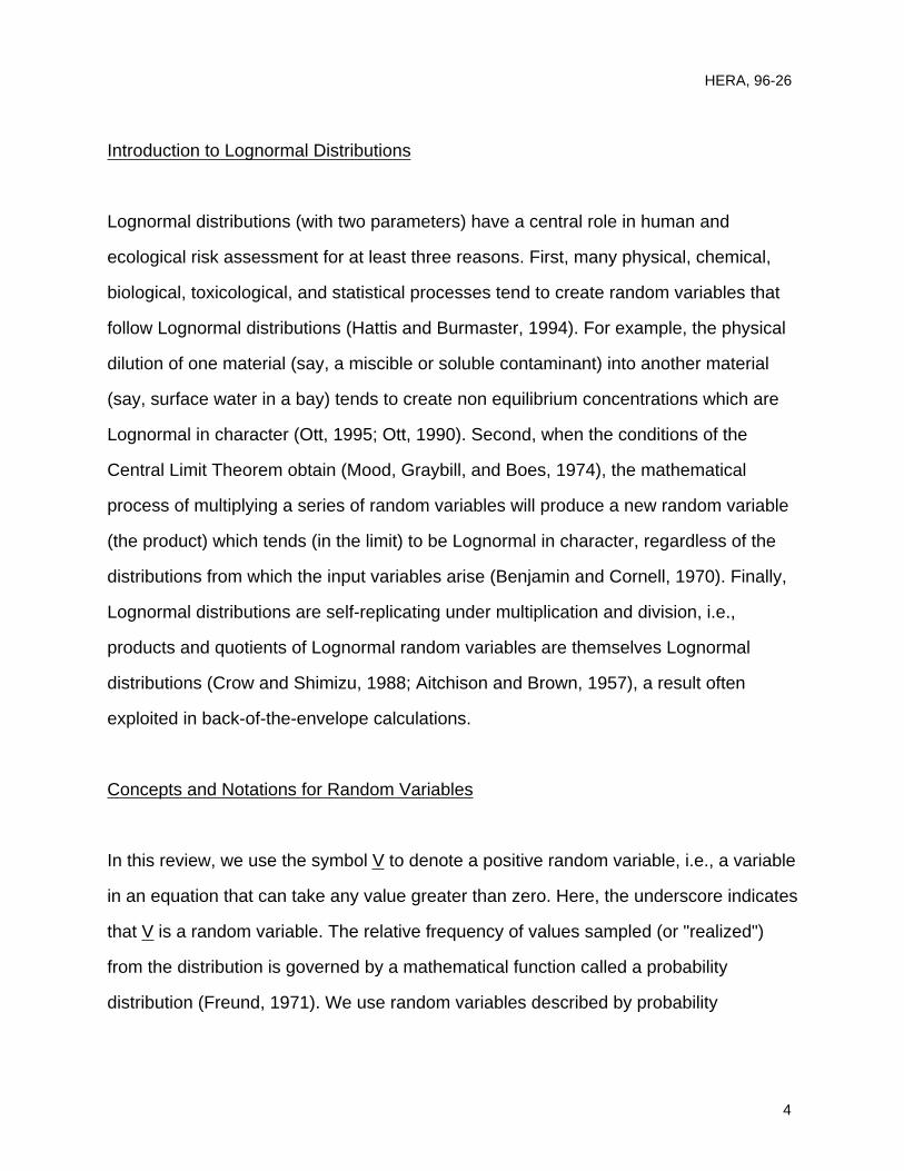
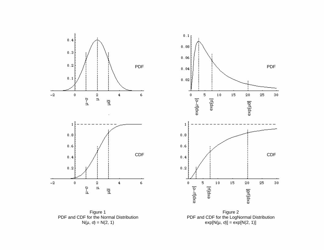
Figure 1 shows graphs for both the PDF and the CDF for an illustrative Normal

distribution, N(µ, σ) = N(2, 1). In Figure 1, the three dotted vertical lines show the values

of the distribution at x = µ and x = µ±σ. As for every Normal distribution, some 68

percent of the area under the PDF occurs between x = µ-σ and x = µ+σ.

The information coded in Eqn 1 is identical to the information coded in Eqn 2:

X ~ exp[ N(µ, σ) ] Eqn 2

where exp[•] denotes the exponential function and N(•, •) again denotes the same

Normal or Gaussian distribution with the same two parameters, mean µ and the

standard deviation σ (with σ > 0) as above. In Eqn 2, X is a Lognormal random variable

(because its logarithm follows a Normal distribution). As earlier, µ is the mean and σ is

the standard deviation of the Normal random variable ln[X], not the Lognormal random

variable X. Many people say that Eqn 2 represents the Lognormal random variable X in

"arithmetic space" or in "linear space." When working with Eqn 2 as the representation

for a Lognormal random variable X, many people refer to N(µ, σ) as the "underlying

6

HERA, 96-26

Normal distribution" or "the Normal distribution in logarithmic space" as a way to

remember its origins.

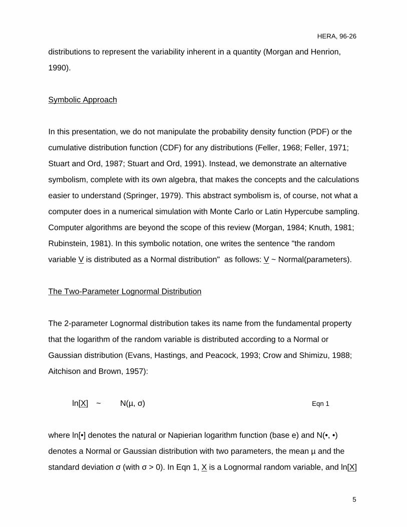
Figure 2 shows graphs for both the PDF and the CDF for the Lognormal distribution,

exp[N(µ, σ)] = exp[N(2, 1)], i.e., the Lognormal distribution for which the Normal

distribution in Figure 1 is the underlying Normal distribution. In Figure 2, the dotted

vertical lines show the values of the Lognormal distribution at x = exp[µ] and x =

exp[µ±σ]. As for every Lognormal distribution, some 68 percent of the area under the

PDF occurs between x = exp[µ-σ] and x = exp[µ+σ].

These two alternate representations for a Lognormal random variable -- Eqn 1 and Eqn

2 -- contain identical information. [EndNote 1] For a particular Lognormal distribution,

the Normal or Gaussian distributions N(µ, σ) in Eqn 1 and Eqn 2 have numerically

identical parameters. The graphs in Figures 1 and 2, then, show two ways to visualize a

particular Lognormal distribution, exp[N(2, 1)]. Figure 1 shows the Normal distribution (in

"logarithmic space") underlying the Lognormal distribution (in "arithmetic space" or linear

space") in Figure 2.

Percentiles of Random Variables ln[X] and X

The two random variables ln[X] and X are related intimately to each other by a common

transformation -- either ln[•] or exp[•] -- depending on the direction of the transformation.

The transformations are 1:1 and monotonic, so the percentiles are closely related by the

same transforms. For example, the 95th percentile for X is the exponential of the 95th

percentile for ln[X], and, in the other direction, the 95th percentile of ln[X] is the natural

logarithm of the 95th percentile of X.

7

HERA, 96-26

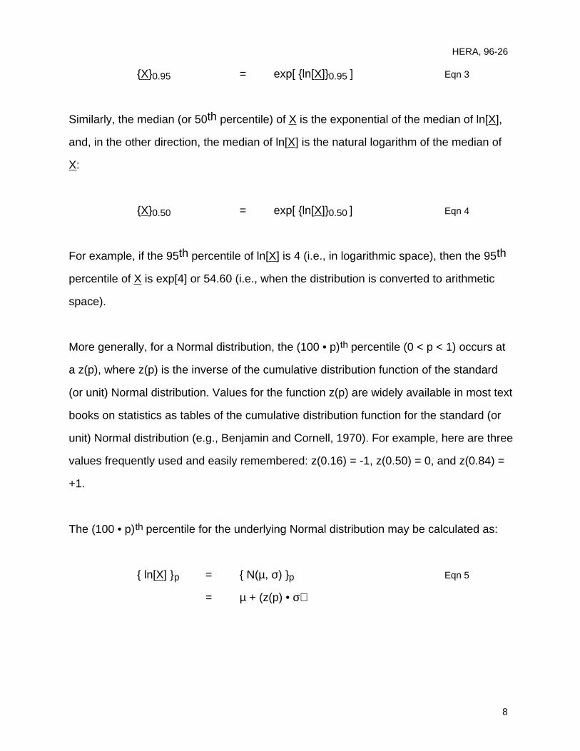
{X}0.95 = exp[ {ln[X]}0.95 ] Eqn 3

Similarly, the median (or 50th percentile) of X is the exponential of the median of ln[X],

and, in the other direction, the median of ln[X] is the natural logarithm of the median of

X:

{X}0.50 = exp[ {ln[X]}0.50 ] Eqn 4

For example, if the 95th percentile of ln[X] is 4 (i.e., in logarithmic space), then the 95th

percentile of X is exp[4] or 54.60 (i.e., when the distribution is converted to arithmetic

space).

More generally, for a Normal distribution, the (100 • p)th percentile (0 < p < 1) occurs at

a z(p), where z(p) is the inverse of the cumulative distribution function of the standard

(or unit) Normal distribution. Values for the function z(p) are widely available in most text

books on statistics as tables of the cumulative distribution function for the standard (or

unit) Normal distribution (e.g., Benjamin and Cornell, 1970). For example, here are three

values frequently used and easily remembered: z(0.16) = -1, z(0.50) = 0, and z(0.84) =

+1.

The (100 • p)th percentile for the underlying Normal distribution may be calculated as:

{ ln[X] }p = { N(µ, σ) }p Eqn 5

= µ + (z(p) • σ)

8

HERA, 96-26

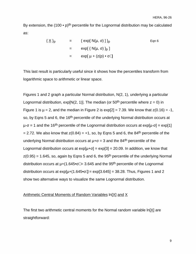
By extension, the (100 • p)th percentile for the Lognormal distribution may be calculated

as:

{ X }p = { exp[ N(µ, σ) ] }p Eqn 6

= exp[ { N(µ, σ) }p ]

= exp[ µ + (z(p) • σ) ]

This last result is particularly useful since it shows how the percentiles transform from

logarithmic space to arithmetic or linear space.

Figures 1 and 2 graph a particular Normal distribution, N(2, 1), underlying a particular

Lognormal distribution, exp[N(2, 1)]. The median (or 50th percentile where z = 0) in

Figure 1 is µ = 2, and the median in Figure 2 is exp[2] = 7.39. We know that z(0.16) = -1,

so, by Eqns 5 and 6, the 16th percentile of the underlying Normal distribution occurs at

µ-σ = 1 and the 16th percentile of the Lognormal distribution occurs at exp[µ-σ] = exp[1]

= 2.72. We also know that z(0.84) = +1, so, by Eqns 5 and 6, the 84th percentile of the

underlying Normal distribution occurs at µ+σ = 3 and the 84th percentile of the

Lognormal distribution occurs at exp[µ+σ] = exp[3] = 20.09. In addition, we know that

z(0.95) = 1.645, so, again by Eqns 5 and 6, the 95th percentile of the underlying Normal

distribution occurs at µ+(1.645•σ) = 3.645 and the 95th percentile of the Lognormal

distribution occurs at exp[µ+(1.645•σ)] = exp[3.645] = 38.28. Thus, Figures 1 and 2

show two alternative ways to visualize the same Lognormal distribution.

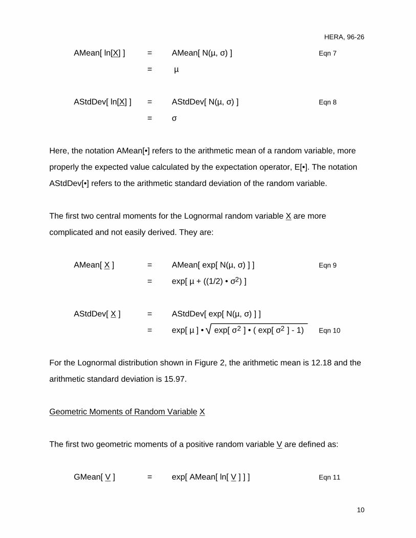
Arithmetic Central Moments of Random Variables ln[X] and X

The first two arithmetic central moments for the Normal random variable ln[X] are

straightforward:

9

HERA, 96-26

AMean[ ln[X] ] = AMean[ N(µ, σ) ] Eqn 7

= µ

AStdDev[ ln[X] ] = AStdDev[ N(µ, σ) ] Eqn 8

= σ

Here, the notation AMean[•] refers to the arithmetic mean of a random variable, more

properly the expected value calculated by the expectation operator, E[•]. The notation

AStdDev[•] refers to the arithmetic standard deviation of the random variable.

The first two central moments for the Lognormal random variable X are more

complicated and not easily derived. They are:

AMean[ X ] = AMean[ exp[ N(µ, σ) ] ] Eqn 9

= exp[ µ + ((1/2) • σ2) ]

AStdDev[ X ] = AStdDev[ exp[ N(µ, σ) ] ]

= exp[ µ ] • exp[ σ2 ] • ( exp[ σ2 ] - 1) Eqn 10

For the Lognormal distribution shown in Figure 2, the arithmetic mean is 12.18 and the

arithmetic standard deviation is 15.97.

Geometric Moments of Random Variable X

The first two geometric moments of a positive random variable V are defined as:

GMean[ V ] = exp[ AMean[ ln[ V ] ] ] Eqn 11

10

HERA, 96-26

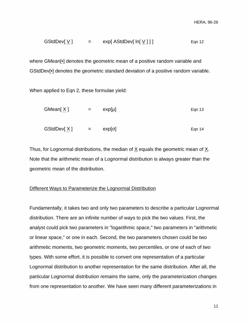
GStdDev[ V ] = exp[ AStdDev[ ln[ V ] ] ] Eqn 12

where GMean[•] denotes the geometric mean of a positive random variable and

GStdDev[•] denotes the geometric standard deviation of a positive random variable.

When applied to Eqn 2, these formulae yield:

GMean[ X ] = exp[µ] Eqn 13

GStdDev[ X ] = exp[σ] Eqn 14

Thus, for Lognormal distributions, the median of X equals the geometric mean of X.

Note that the arithmetic mean of a Lognormal distribution is always greater than the

geometric mean of the distribution.

Different Ways to Parameterize the Lognormal Distribution

Fundamentally, it takes two and only two parameters to describe a particular Lognormal

distribution. There are an infinite number of ways to pick the two values. First, the

analyst could pick two parameters in "logarithmic space," two parameters in "arithmetic

or linear space," or one in each. Second, the two parameters chosen could be two

arithmetic moments, two geometric moments, two percentiles, or one of each of two

types. With some effort, it is possible to convert one representation of a particular

Lognormal distribution to another representation for the same distribution. After all, the

particular Lognormal distribution remains the same, only the parameterization changes

from one representation to another. We have seen many different parameterizations in

11

HERA, 96-26

the literature, and we have seen some authors even use several different

parameterizations in one article. Given the infinite number of representations for just

one Lognormal distribution, the possibilities for confusion and mistakes are boundless.

In this review, we emphasize the central importance of µ and σ, the mean and standard

deviation of the Normal or Gaussian distributions in "logarithmic space," as a consistent

and powerful way to parameterize a Lognormal distribution for X. We strongly

recommend this practice.

However, in writing articles in the refereed literature, many other authors often choose

different parameterizations. Many authors prefer to parameterize a Lognormal

distribution for X in terms of its geometric mean and its geometric standard deviation, or

equivalently, in terms of its median and its geometric standard deviation.

Fewer authors parameterize a Lognormal distribution for X in terms of its arithmetic

mean and arithmetic standard deviation. We find this usage problematic because the

arithmetic mean of X and arithmetic standard deviation of X are numerically unstable

when working with data or simulations.

Given the formulae in the earlier sections, the reader may solve the equations pairwise

to convert one parameterization to another.

To reduce confusion, we also mention that some authors prefer to use common

logarithms (base 10) in the fundamental representations:

log10[ X ] ~ N(µ10, σ10) Eqn 1'

12

HERA, 96-26

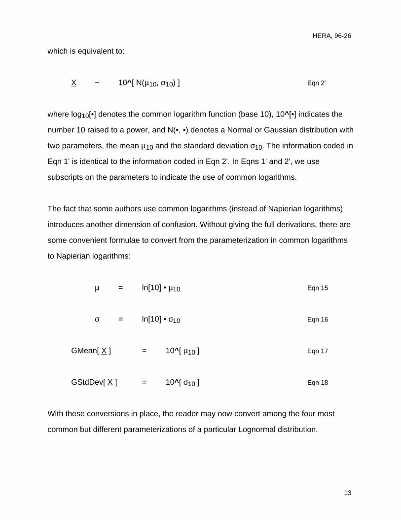
which is equivalent to:

X ~ 10^[ N(µ10, σ10) ] Eqn 2'

where log10[•] denotes the common logarithm function (base 10), 10^[•] indicates the

number 10 raised to a power, and N(•, •) denotes a Normal or Gaussian distribution with

two parameters, the mean µ10 and the standard deviation σ10. The information coded in

Eqn 1' is identical to the information coded in Eqn 2'. In Eqns 1' and 2', we use

subscripts on the parameters to indicate the use of common logarithms.

The fact that some authors use common logarithms (instead of Napierian logarithms)

introduces another dimension of confusion. Without giving the full derivations, there are

some convenient formulae to convert from the parameterization in common logarithms

to Napierian logarithms:

µ = ln[10] • µ10 Eqn 15

σ = ln[10] • σ10 Eqn 16

GMean[ X ] = 10^[ µ10 ] Eqn 17

GStdDev[ X ] = 10^[ σ10 ] Eqn 18

With these conversions in place, the reader may now convert among the four most

common but different parameterizations of a particular Lognormal distribution.

13

HERA, 96-26

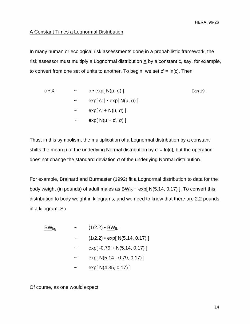
A Constant Times a Lognormal Distribution

In many human or ecological risk assessments done in a probabilistic framework, the

risk assessor must multiply a Lognormal distribution X by a constant c, say, for example,

to convert from one set of units to another. To begin, we set c' = ln[c]. Then

c • X ~ c • exp[ N(µ, σ) ] Eqn 19

~ exp[ c' ] • exp[ N(µ, σ) ]

~ exp[ c' + N(µ, σ) ]

~ exp[ N(µ + c', σ) ]

Thus, in this symbolism, the multiplication of a Lognormal distribution by a constant

shifts the mean µ of the underlying Normal distribution by c' = ln[c], but the operation

does not change the standard deviation σ of the underlying Normal distribution.

For example, Brainard and Burmaster (1992) fit a Lognormal distribution to data for the

body weight (in pounds) of adult males as BWlb ~ exp[ N(5.14, 0.17) ]. To convert this

distribution to body weight in kilograms, and we need to know that there are 2.2 pounds

in a kilogram. So

BWkg ~ (1/2.2) • BWlb

~ (1/2.2) • exp[ N(5.14, 0.17) ]

~ exp[ -0.79 + N(5.14, 0.17) ]

~ exp[ N(5.14 - 0.79, 0.17) ]

~ exp[ N(4.35, 0.17) ]

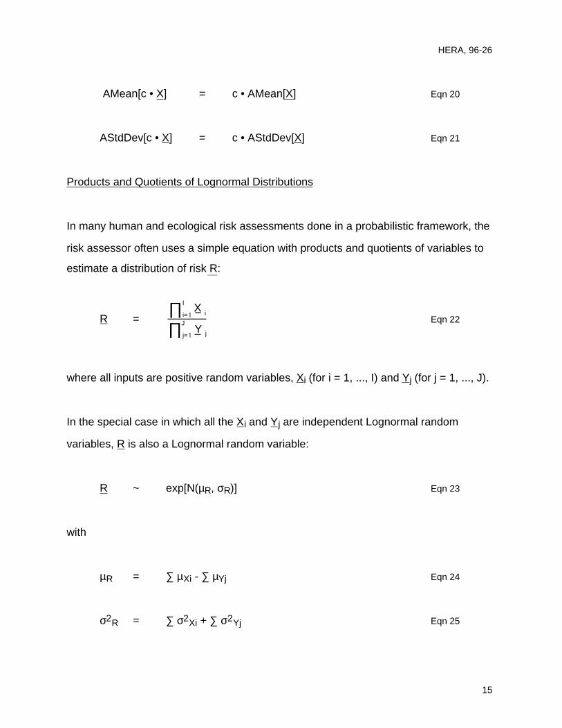
Of course, as one would expect,

14

HERA, 96-26

AMean[c • X] = c • AMean[X] Eqn 20

AStdDev[c • X] = c • AStdDev[X] Eqn 21

Products and Quotients of Lognormal Distributions

In many human and ecological risk assessments done in a probabilistic framework, the

risk assessor often uses a simple equation with products and quotients of variables to

estimate a distribution of risk R:

R =iX

i= 1

I∏jY

j= 1

J∏Eqn 22

where all inputs are positive random variables, Xi (for i = 1, ..., I) and Yj (for j = 1, ..., J).

In the special case in which all the Xi and Yj are independent Lognormal random

variables, R is also a Lognormal random variable:

R ~ exp[N(µR, σR)] Eqn 23

with

µR = ∑ µXi - ∑ µYj Eqn 24

σ2R = ∑ σ2Xi + ∑ σ2Yj Eqn 25

15

HERA, 96-26

This result demonstrates both a fundamental property of independent Lognormal

distributions and the felicity of parameterizing the distributions in terms of the mean and

standard deviation of the underlying Normal distribution. In the first equation for µR, the

contribution from the variables in the denominator enter preceded by a minus sign, but,

in the second equation for σ2R, the contribution from the variables in the denominator

enter preceded by a plus sign.

A Simplified Way to Fit Lognormal Distributions to Data

We use the symbols x1, x2, ..., xn, ... , xN to denote a set of N values sampled or

realized from the random variable X. Even though X is a random variable, each of the N

realizations from it, denoted xn (for n = 1, ..., N), is a point value.

First, before beginning a formal fitting process below, use exploratory data analysis and

visualization to plot the data in many different ways on many different axes (Cleveland,

1994; Cleveland, 1993; Tukey, 1977). Modern commercial software (e.g., Systat, 1992)

running on a desktop computer makes this exploratory data analysis fast, fun, and

indispensable. We emphasize the critical importance of this approach.

When it comes time to fit a Lognormal distribution to a set of data x1, ..., xN, we

recommend an 8-step, simplified process. In this review, we do not consider more

complicated situations such as fitting a distribution to a data set with censored or

truncated values, e.g., chemical concentrations reported as BDL (below the detection

limit), although such fits are easily accomplished using the Method of Maximum

Likelihood (Keeping, 1995; Edwards, 1992) or other methods (Travis and Land, 1990).

16

HERA, 96-26

Step 1: Check to see if each of the values xn > 0 for n = 1, ... , N. If some values are

zero or negative, Stop, because a 2-parameter Lognormal distribution cannot fit the

data. If all xn are positive, Go to Step 2, because a 2-parameter Lognormal distribution

may fit the data.

Step 2: Take the natural logarithms of the xn values for n = 1, ..., N. Work in "logarithmic

space" with the ln[xn] values in all of the remaining steps in this fitting process. Go to

Step 3.

Step 3: Plot a histogram of the ln[xn] values. If the histogram of the ln[xn] values is

asymmetric by having a long tail to the left or the right, Stop, because a 2-parameter

Lognormal distribution cannot fit the data. If the histogram of the ln[xn] values is

symmetric, Go to Step 4, because a 2-parameter Lognormal distribution may fit the

data.

Step 4: Plot a Lognormal probability plot with z(p) on the abscissa and ln[xn] on the

ordinate (see Section 13, below). If the N points plot in a curved line on these axes,

Stop, because a 2-parameter Lognormal distribution cannot fit the data. If the N points

plot in an approximately straight line on these axes, Go to Step 5, because a 2-

parameter Lognormal distribution will fit the data. Include this graph in your final report.

Some authors (e.g., D'Agostino and Stephens, 1986) and some commercial software

packages (e.g., Systat, 1992) transpose the axes by plotting ln[xn] on the abscissa and

z(p) on the ordinate.

Step 5: Using ordinary least-squares regression, fit a straight line to the data plotted on

the Lognormal probability plot with z(p) on the abscissa and ln[xn] on the ordinate. The

line will have this functional form, with z as the independent variable in the regression:

17

HERA, 96-26

line = a + (b • z) Eqn 26

where a is the intercept of the fitted line when z = 0 and b is the slope of the fitted line.

Include this graph in your final report, along with all the goodness of fit statistics for the

regression. Then, ˆ µ = a is a good estimate for the parameter µ in Eqns 1 and 2 and ˆ σ =

b is a good estimate for σ in Eqns 1 and 2. Usually the regression package will report

confidence internals for a and b. Go to Step 6. In this Step 5, a regression line fit to the

transposed Lognormal probability plot with ln[xn] on the abscissa and z(p) on the

ordinate will not give correct estimates for ˆ µ and ˆ σ because the regression does not

have the proper independent variable.

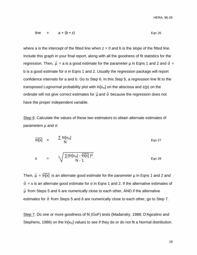
Step 6: Calculate the values of these two estimators to obtain alternate estimates of

parameters µ and σ:

ln[x] =∑ ln[xn]

N Eqn 27

s = ∑(ln[xn] - ln[x] )2

N - 1 Eqn 28

Then, ˆ µ = ln[x] is an alternate good estimate for the parameter µ in Eqns 1 and 2 and

ˆ σ = s is an alternate good estimate for σ in Eqns 1 and 2. If the alternative estimates of

ˆ µ from Steps 5 and 6 are numerically close to each other, AND if the alternative

estimates for ˆ σ from Steps 5 and 6 are numerically close to each other, go to Step 7.

Step 7: Do one or more goodness of fit (GoF) tests (Madansky, 1988; D'Agostino and

Stephens, 1986) on the ln[xn] values to see if they do or do not fit a Normal distribution.

18

HERA, 96-26

Even though these methods do not visualize the data and are not as robust as the

probability plot above, discuss the results of these tests in your final report. Go to Step

8.

Step 8: Discuss the adequacy of the fit compared to the use of the Lognormal

distribution in a narrative in your final report. Note any outliers, problems, or issues.

State the conditions and circumstances in which the results apply; also state the

conditions and circumstances in which the results do not apply. Discuss alternative fits

and conduct numerical experiments to see if use of an alternative fit would lead to a

different decision in the real world.

Discussion of the Simplified 8-Step Method

After the initial exploratory data analysis and data visualization, we recommend an 8-

step, simplified process for fitting a Lognormal distribution to data. First, we recommend

that the analyst work with the ln[xn] values to fit the parameters µ and σ of the

underlying Normal distribution -- precisely because working with the untransformed xn

values is numerically unstable in most cases. Second, we recommend that the analyst

complete all 8 steps in entirety -- precisely because we have seen egregious mistakes

when an analyst ignores a particular step. Third, visualize! visualize!! visualize!!! in each

step in the procedure. These 8 steps form the framework of many publications in the

refereed literature (e.g., Roseberry and Burmaster, 1992; Murray and Burmaster, 1992)

Although we have found that these 8 steps work well for many univariate data sets and

for the marginal distributions of many multivariate data sets, the methods will not work to

fit a multivariate distribution to multivariate data that may include non negligible

correlations and/or dependencies. Finally, although this recommended 8-step process

19

HERA, 96-26

rests on powerful and recognized statistical techniques with long pedigrees -- i.e.,

probability plots, the method of moments, and the method of maximum likelihood --

there are other powerful and accepted techniques not included -- e.g., maximum

entropy methods (Kapur and Kesavan, 1992) and model-free curve estimation (Tarter

and Lock, 1993).

Numerical Simulations with Lognormal Variables

When starting a numerical simulation with Lognormal random variables, we recommend

a two-step process:

First, generate or simulate values for ln[X] by drawing values from the underlying

Normal distribution N(µ, σ) in logarithmic space. Second, exponentiate those values for

ln[X] to obtain values for X from the Lognormal distribution exp[N(µ, σ)] in linear space.

This two-step process basically reverses the 8-step fitting process just presented in

Section 11.0 above. For example, when using a commercial software product in

conjunction with a spreadsheet on a desktop computer, the analyst would simulate the

underlying Normal distribution, N(µ, σ), in one cell and then exponentiate it in an

adjacent cell. This two-step process gives the analyst much more control of the

simulation at a negligible penalty in speed. It also helps the reviewer, e.g., a reviewer at

a regulatory agency, check for errors.

Many common software packages, [e.g., Crystal Ball™ (Decisioneering, 1992),

Demos™ (Lumina, 1993), RiskQ™ (Bogen, 1992; Murray and Burmaster, 1993)] offer

pre-programmed routines or functions that sample a Lognormal distribution in one step

20

HERA, 96-26

instead of two. We recommend that an analyst not use these features until she or he is

seasoned and highly experienced in the pitfalls of simulation.

Why not use such tempting features? In our experience, each different software

package uses a different parameterization for the Lognormal distribution. This in itself is

not necessarily bad, only confusing, especially when the Users Manuals are often less

than clear on the chosen parameterization. If a neophyte analyst misinterprets the User

Manual -- say by specifying the geometric mean of a distribution when the software

expects the arithmetic mean of the distribution as an input -- the overall simulation may

be wrong by an order of magnitude or more. Moreover, a reviewer would have an

extremely difficult time catching this fundamental error. GIGO [EndNote 2] happens all

too often in numerical simulations because the analyst does not understand the tools in

use and does not use numerical experiments or the algebra of random variables

(Springer, 1979) to check the first set of simulations. Once an analyst has months of

experience with the two-step process recommended here, she or he may want to

experiment with the built-in features of her or his chosen software package. Caveat

emptor! as always.

Introduction to Lognormal Probability Plots

Statisticians have designed "probability plots" for many kinds of probability distributions,

e.g., Normal, Lognormal, and Exponential distributions, but no probability plots exist for

some distributions, e.g, Gamma distributions. For a general discussion of probability

plots, see, e.g., Chapter 1 in Goodness-of-Fit Techniques (D'Agostino and Stephens,

1986).

21

HERA, 96-26

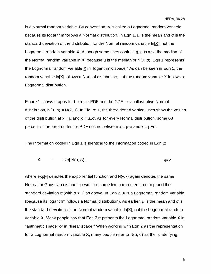
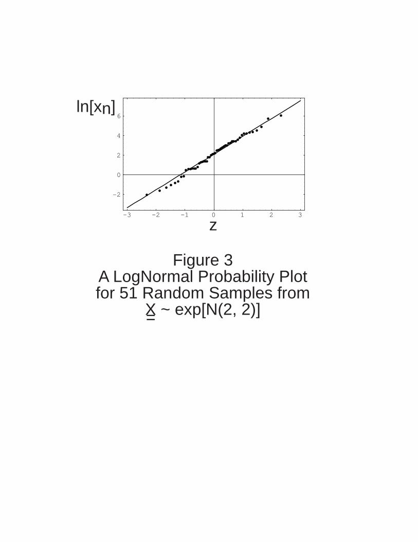
Lognormal probability plots have many uses in probabilistic risk assessments precisely

because Lognormal distributions occur naturally and are ubiquitous in probabilistic risk

assessments. Figure 3 shows a typical Lognormal probability plot with a straight line fit

by ordinary least squares regression.

By definition, a probability plot is any 2D graph (with special or transformed axes) on

which values realized from the corresponding probability distribution plot in a straight

line (Benjamin and Cornell, 1970). For example, a set of values that are randomly

sampled from an exponential distribution will plot in a straight line on an exponential

probability plot (or in an almost straight line, given the randomness of the sample). As

another example, data measured from many physical, chemical, or biological processes

follow Lognormal distributions in theory and in practice (Hattis and Burmaster, 1994).

In this review, we show how to create a Lognormal probability plot using only a

spreadsheet program. As a practical matter, we think all risk assessors need to know

how to plot their own probability plot for three reasons. First, it teaches important skills.

Second, it allows the risk assessor to extend the technique to develop and plot data on

related graphs, e.g., a CubeRoot probability plot. Third, it gives the risk assessor a way

to correct a flaw in many commercial statistics programs (e.g., Systat, 1992) that

reverse (transpose) the axes.

In this presentation, we do not consider making a Lognormal probability plot for a set of

values or data that include censored or truncated entries, e.g., chemical concentrations

reported as BDL (below the detection limit), although such plots are sometimes easily

accomplished if only a few values are truncated or censored (see, e.g., Travis and Land,

1990).

22

HERA, 96-26

The Functions p(z) and z(p)

The Function p(z)

Most introductory books on probability or statistics introduce the "standard" or "unit"

Normal distribution with a mean µ = 0 and a standard deviation σ = 1. Here, we write the

unit Normal distribution as N(0, 1) (Freund, 1971).

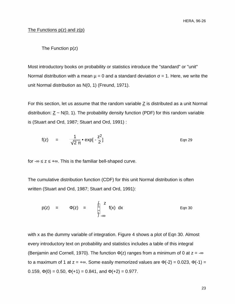
For this section, let us assume that the random variable Z is distributed as a unit Normal

distribution: Z ~ N(0, 1). The probability density function (PDF) for this random variable

is (Stuart and Ord, 1987; Stuart and Ord, 1991) :

f(z) =1

2 π • exp[ -

z2

2 ] Eqn 29

for -∞ ≤ z ≤ +∞. This is the familiar bell-shaped curve.

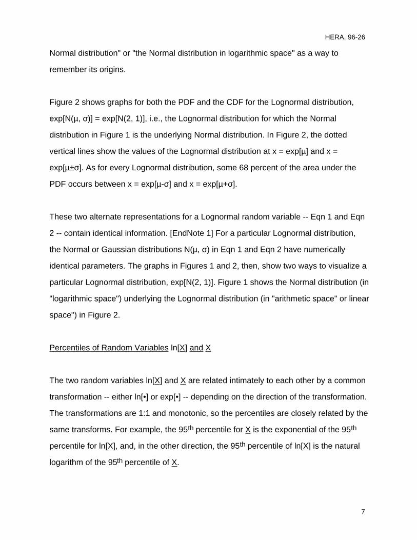
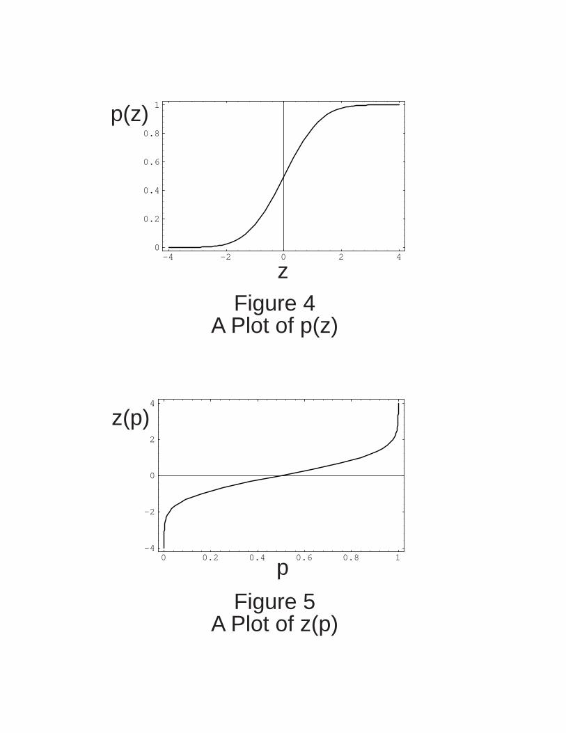
The cumulative distribution function (CDF) for this unit Normal distribution is often

written (Stuart and Ord, 1987; Stuart and Ord, 1991):

p(z) = Φ(z) =⌡⌠

-∞

z f(x) dx Eqn 30

with x as the dummy variable of integration. Figure 4 shows a plot of Eqn 30. Almost

every introductory text on probability and statistics includes a table of this integral

(Benjamin and Cornell, 1970). The function Φ(z) ranges from a minimum of 0 at z = -∞

to a maximum of 1 at z = +∞. Some easily memorized values are Φ(-2) = 0.023, Φ(-1) =

0.159, Φ(0) = 0.50, Φ(+1) = 0.841, and Φ(+2) = 0.977.

23

HERA, 96-26

We interpret 100 • Φ(z) as computing the percentile of the unit Normal distribution

associated with a particular z value for -∞ ≤ z ≤ +∞. Under this interpretation, we see

that the z = -1 corresponds to the 16th percentile, z = 0 corresponds to the 50th

percentile (the median), and z = +1 corresponds to the 84th percentile. Thus, we can

use Eqn 30 to compute the percentiles for a unit Normal distribution.

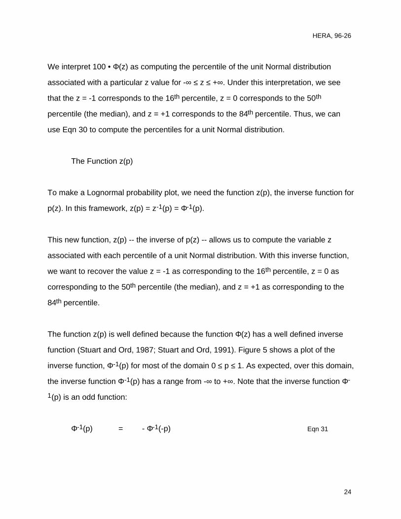
The Function z(p)

To make a Lognormal probability plot, we need the function z(p), the inverse function for

p(z). In this framework, z(p) = z-1(p) = Φ-1(p).

This new function, z(p) -- the inverse of p(z) -- allows us to compute the variable z

associated with each percentile of a unit Normal distribution. With this inverse function,

we want to recover the value z = -1 as corresponding to the 16th percentile, z = 0 as

corresponding to the 50th percentile (the median), and z = +1 as corresponding to the

84th percentile.

The function z(p) is well defined because the function Φ(z) has a well defined inverse

function (Stuart and Ord, 1987; Stuart and Ord, 1991). Figure 5 shows a plot of the

inverse function, Φ-1(p) for most of the domain 0 ≤ p ≤ 1. As expected, over this domain,

the inverse function Φ-1(p) has a range from -∞ to +∞. Note that the inverse function Φ-

1(p) is an odd function:

Φ-1(p) = - Φ-1(-p) Eqn 31

24

HERA, 96-26

Computing the Function z(p)

To make a Lognormal probability plot, we need values for the function z(p) evaluated at

each of the sampled or measured values. There are generally two ways to do this.

First, from standard tables. It is easy but tedious to read standard tables p(z)

backwards, i.e., to read values for z(p) from tables of p(z) (e.g., Benjamin and Cornell,

1970).

Second, by computation. Many commercial spreadsheet products and many other

commercial software packages calculate the function z(p). For example, in Microsoft

Excel™ 5.0 for the Macintosh and for Windows (Microsoft, 1994), the built-in function

called NORMSINV(probability) computes z(p) for -∞ < p < +∞. In Mathematica™

(Wolfram, 1991), the user may define a function z(p) in terms of functions built into the

software:

z[p_] := Sqrt[2] InverseErf[2 p - 1] Eqn 32

With the mathematical formulae available in standard mathematical handbooks (e.g,

Abramowitz and Stegun, 1964), the analyst can evaluate the function z(p) by knowing

the right built-in function or by writing a short subroutine. Also, Bogen (1993) has

published a fast intermediate-precision approximation for z(p).

Plotting a Lognormal Probability Plot

In this section, we again use the symbols x1, x2, ..., xn, ... , xN to denote a set of N

values sampled (or realized or measured) from a random variable X. We want to see if

25

HERA, 96-26

these xn values come from a Lognormal distribution. Even though X is a random

variable, each of the N realizations from it, denoted xn (for n = 1, ..., N), is a point value.

We recommend a 6-step process to make a Lognormal probability plot to visualize a set

of N values x1, x2, ..., xN. [EndNote 3]

Step 1: Sort the N values from the smallest to the largest, so that x1 ≤ x2 ≤ .... ≤ xN. This

presentation allows for some ties among the N values. In the rest of this algorithm for

Lognormal probability plots, we assume that the N values are sorted from the smallest

to the largest.

Step 2: Check to see if each of the values xn > 0 for n = 1, ... , N. If some values are

zero or negative, Stop, because a 2-parameter Lognormal distribution cannot fit the

data. If all xn are positive, Go to Step 3, because a 2-parameter Lognormal distribution

may fit the data.

Step 3: Take the natural logarithms of the xn values for n = 1, ..., N. Work in "logarithmic

space" with the ln[xn] values in all of the remaining steps in this fitting process. Go to

Step 4. [EndNote 4]

Step 4: For each of the N data points, compute an empirical cumulative probability as:

pn =n - 0.5

N for n = 1, 2, ..., N. Eqn 33

This simple formula works well in most cases, but the statistical literature contains

discussions of other formulae for computing the empirical cumulative probability for use

in probability plots.

26

HERA, 96-26

Step 5: Compute z(pn) for n = 1, 2, ... , N. [EndNote 5]

Step 6: Plot the points with coordinates {z(pn), ln[xn]} for n = 1, 2, ... , N on a Lognormal

probability plot with z(pn) on the abscissa and ln[xn] on the ordinate. If the N points plot

in a curved line on these axes, Stop, because a 2-parameter Lognormal distribution

cannot fit the data. [EndNote 6] If the N points plot in an approximately straight line on

these axes, Continue, because a 2-parameter Lognormal distribution will fit the data.

[EndNote 7] Include this graph in the final report. Some authors (e.g., D'Agostino and

Stephens, 1986) and some commercial software packages (e.g., Systat, 1992)

transpose the axes.

Discussion of Lognormal Probability Plots

A Lognormal probability plot is a powerful technique because the plot allows the analyst

to see all the data in comparison to a full Lognormal distribution (and because it

combines exploratory data analysis with parameter estimation). Data points falling on a

straight line on a Lognormal probability plot imply that a Lognormal distribution will fit the

data with high fidelity (e.g., Figure 1), and data points falling near a straight line (with no

systematic curvature) imply that a Lognormal distribution will fit the data with good

fidelity. In such a situation, the analyst may estimate the two parameters of the best-fit

Lognormal distribution by using ordinary least squares to fit a straight line to the data

and to compute the regression coefficients. Lognormal probability plots do have a major

limitation, however. By design, each quantile on a Lognormal probability plot depends

on the lower ones, so that the plotting positions of the independent variable in the linear

regression are not independent. When in doubt, the analyst may use the Method of

27

HERA, 96-26

Maximum Likelihood (Edwards, 1992) to estimate the two best-fit parameters for the

Lognormal distribution.

With a Lognormal probability plot, the analyst can see the nature and the quality of the

fit over the whole distribution, and she or he can use any systematic departures from a

fit to investigate other models for the data (D'Agostino, Belanger, and D'Agostino, 1990).

For example, Figure 4 in Brainard and Burmaster (1992) shows how a systematic

curvature of data points plotted on a Lognormal probability plot led to a new

understanding of the distribution of women's body weights. Traditional GoF tests do not

let the analyst visualize the data. With a traditional GoF test, one or two errant data

points may lead to a conclusion that a Lognormal distribution does not fit the data, even

though a Lognormal probability plot may show that the fit is excellent over the range of

interest.

28

HERA, 96-26

EndNotes

1. Eqn 1 and Eqn 2 are unrealistic models for certain physical, chemical, or biological phenomena

insofar as they allow random variable X to increase without bound. It may be necessary to

truncate the model in Eqns 1 or 2 at a finite value for the upperbound of the phenomenon.

2. In the early days of electronic computers, GIGO stood for the phrase "Garbage In, Garbage Out."

Today, GIGO too often stands for the phrase "Garbage In, Gospel Out."

3. A Logprobit plot is almost identical (Finney, 1971), except the abscissa is translated 5 units.

4. Some authors (e.g., Hattis and Burmaster, 1994) use common logarithms (to the base 10) in

making Lognormal probability plots. This convention is internally consistent, but any parameters

estimated by linear regression on such a plot require conversion if the rest of the analysis uses

Napierian logarithms.

5. Given that z(p) is an odd function, z(p1) = -z(pN) when pn = n - 0.5

N for n = 1, 2, ..., N.

6. If the points tend to follow a smooth, nonlinear curve on a Lognormal probability plot, D'Agostino

and Stephens (1986) suggest other types of probability plots to consider. For example, the data

may plot in a straight line on a Normal probability plot, a CubeRoot probability plot, or another

PowerTransformed probability plot.

7. In our experience, an R2 ≥ 0.95 with no systematic curvature implies an adequate fit. But note:

the R2 for a regression on a probability plot is not a substitute for the Wilks-Shapiro test for the

adequacy of a fit (Gilbert, 1987).

29

HERA, 96-26

Dedication and Acknowledgments

We dedicate this manuscript in the memory of Jerome Bert Wiesner.

Alceon Corporation funded this work.

We thank two anonymous reviewers for excellent suggestions for improvements to this

manuscript.

30

HERA, 96-26

References

Abramowitz, M. and Stegun, I.A., Eds. 1964. Handbook of Mathematical Functions with Formulas,

Graphs, and Mathematical Tables, National Bureau of Standards, Applied Mathematics Series

Number 55, Issued June 1964, Tenth Printing with corrections in December 1972, US

Government Printing Office, Washington, DC.

Aitchison, J. and Brown, J.A.C. 1957. The Lognormal Distribution, Cambridge University Press,

Cambridge, UK.

AIHC (American Industrial Health Council). 1994. Exposure Factors Source Book, Washington, DC.

Benjamin, J.R. and Cornell, C.A. 1970. Probability, Statistics, and Decision for Civil Engineers, McGraw

Hill, New York, NY.

Bogen, K.T. 1993. An Intermediate-Precision Approximation of the Inverse Cumulative Normal

Distribution, Communications in Statistics, Simulation and Computation, Volume 23, Number 3,

pp 797 - 801

Bogen, K.T. 1992. RiskQ: An Interactive Approach to Probability, Uncertainty, and Statistics for Use with

Mathematica, Reference Manual, UCRL-MA-110232 Lawrence Livermore National Laboratory,

University of California, Livermore, CA, July 1992.

Brainard, J. and Burmaster, D.E. 1992. Bivariate Distributions for Height and Weight of Men and Women

in the United States, Risk Analysis, 1992, Vol. 12, No. 2, pp 267-275

31

HERA, 96-26

Burmaster, D.E. and Bloomfield, L.R. 1996. Mathematical Properties of the Risk Equation When

Variability is Present, Human and Ecological Risk Assessment, Volume 2, Number 2, pp 348 -

355.

Cleveland, W.S. 1993. Visualizing Data, AT&T Bell Laboratories, Hobart Press, Summit, NJ.

Cleveland, W.S. 1994. The Elements of Graphing Data, AT&T Bell Laboratories, Hobart Press, Summit,

NJ.

Crow, E.L. and Shimizu, K., Eds. 1988. Lognormal Distributions, Theory and Applications, Marcel Dekker,

New York, NY.

D'Agostino, R.B., Belanger, A., and D'Agostino, Jr., R.B. 1990. A Suggestion for Using Powerful and

Informative Tests of Normality, American Statistician, Volume 44, Number 4, pp 316 - 321.

D'Agostino, R.B. and Stephens, M.A. 1986. Goodness-of-Fit Techniques, Marcel Dekker, New York, NY.

Decisioneering, Inc., 1992. Users Manual for Crystal Ball, Denver, CO.

Edwards, A.W.F. 1992. Likelihood, John Hopkins University Press, Baltimore, MD.

Evans, M., Hastings, N. and Peacock, B. 1993. Statistical Distributions, Second Edition, John Wiley and

Sons, New York, NY.

Feller, W. 1968. An Introduction to Probability Theory and Its Applications, Volume I, John Wiley, New

York, NY.

32

HERA, 96-26

Feller, W. 1971. An Introduction to Probability Theory and Its Applications, Volume II, John Wiley, New

York, NY.

Finney, D.J. 1971. Probit Analysis, Cambridge Press, Cambridge, UK.

Freund, J.E. 1971. Mathematical Statistics, Second Edition, Prentice-Hall, Englewood Cliffs, NJ.

Gilbert, R.O. 1987. Statistical Methods for Environmental Pollution Monitoring, Van Nostrand Reinhold,

New York, NY.

Hattis, D.B. and Burmaster, D.E. 1994. Assessment of Variability and Uncertainty Distributions for

Practical Risk Assessments, Risk Analysis, Volume 14, Number 5, pp 713 - 730.

Kapur, J.N. and Kesavan, H.K. 1992. Entropy Optimization: Principles with Applications, Academic Press,

Harcourt Brace Jovanovich, Boston, MA..

Keeping, E.S. 1995. Introduction to Statistical Inference, Dover, New York, NY.

Knuth, D.E. 1981. The Art of Computer Programming, Seminumerical Algorithms, Volume 2, Second

Edition, Addison-Wesley, Reading, MA.

Lumina Decision Systems. 1993. Users Manual for DEMOS™, Los Altos, CA.

Madansky, A.,1988. Prescriptions for Working Statisticians, Springer-Verlag, New York, NY.

Microsoft Corporation. 1994. Microsoft Excel 5 Worksheet Function Reference, Microsoft Press,

Redmond, WA.

33

HERA, 96-26

Mood, A.M., Graybill, F.A., and Boes, D.C. 1974. Introduction to the Theory of Statistics, Third Edition,

McGraw Hill, New York, NY.

Morgan, J.T.M. 1984. Elements of Simulation, Chapman and Hall, London, UK.

Morgan, M.G. and Henrion, M. 1990. Uncertainty, Cambridge University Press, Cambridge, UK.

Murray, D.M., and Burmaster, D.E. 1992. Estimated Distributions for Total Body Surface Area of Men and

Women in the United States, Journal of Exposure Analysis and Environmental Epidemiology

Volume 2, Number 4, pp 451 - 461.

Murray, D.M. and Burmaster, D.E. 1993. Review of RiskQ: An Interactive Approach to Probability,

Uncertainty, and Statistics for Use with Mathematica, Risk Analysis, Volume 13, Number 4, pp

479 - 482.

Ott, W.R. 1995. Environmental Statistics and Data Analysis, Lewis Publishers, Boca Raton, FL.

Ott, W.R. 1990. A Physical Explanation of the Lognormality of Pollutant Concentrations, Journal of the Air

and Waste Management Association, Volume 40, pp 1378 et seq.

Roseberry, A.M., and Burmaster, D.E. 1992. Lognormal Distributions for Water Intake by Children and

Adults, Risk Analysis, Volume 12, Number 1, pp 99 - 104.

Rubinstein, R.Y. 1981. Simulation and the Monte Carlo Method, John Wiley and Sons, New York, NY.

Springer, M.D. 1979. The Algebra of Random Variables, John Wiley and Sons, New York, NY.

34

HERA, 96-26

Stuart, A. and Ord, J.K. 1987. Kendall's Advanced Theory of Statistics, Fifth Edition of Volume 1, Oxford

University Press, New York, NY.

Stuart, A. and Ord, J.K. 1991. Kendall's Advanced Theory of Statistics, Fifth Editions of Volume 2, Oxford

University Press, New York, NY.

Systat, Inc., 1992, Users Manual, Evanston, IL.

Tarter, M.E. and Lock, M.D. 1993. Model-Free Curve Estimation, Chapman and Hall, New York, NY.

Travis, C.C. and Land, M.L. 1990. Estimating the Mean of Data Sets with NonDetectable Values,

Environmental Science and Technology, Volume 24, Number 7, pp 961 - 962.

Tukey, J.W. 1977. Exploratory Data Analysis, Addison-Wesley, Reading, MA.

Wolfram, S. 1991. Mathematica™, A System for Doing Mathematics by Computer, Second Edition,

Addison-Wesley, Redwood City, CA.

35

µ−σ µ

µ+σ

µ−σ µ

µ+σ

exp[

µ−σ]

exp[

µ]

exp[

µ+σ]

exp[

µ−σ]

exp[

µ]

exp[

µ+σ]

Figure 1PDF and CDF for the Normal Distribution

N(µ, σ) = N(2, 1)

PDF

CDF

Figure 2PDF and CDF for the LogNormal Distribution

exp[N(µ, σ)] = exp[N(2, 1)]

PDF

CDF

-3 -2 -1 0 1 2 3

-2

0

2

4

6

z

ln[xn]

Figure 3A LogNormal Probability Plotfor 51 Random Samples from

X ~ exp[N(2, 2)]=

-4 -2 0 2 40

0.2

0.4

0.6

0.8

1

0 0.2 0.4 0.6 0.8 1-4

-2

0

2

4

z

p(z)

z(p)

p

Figure 4A Plot of p(z)

Figure 5A Plot of z(p)