Embed Size (px)
Citation preview
NONLINEAR FINITE ELEMENT ANALYSIS OF COLUMNS
by
RAJKIRAN MUPPAVARAPU
Presented to the Faculty of the Graduate School of
The University of Texas at Arlington in Partial Fulfillment
of the Requirements
for the Degree of
MASTER OF SCIENCE IN AEROSPACE ENGINEERING
THE UNIVERSITY OF TEXAS AT ARLINGTON
May 2011

ii
ACKNOWLEDGEMENTS
I would like to first thank Dr. Kent Lawrence for his guidance throughout the project. He
has been a big source of inspiration for me. I would also like to thank Dr. B.P. Wang and Dr. S.
Nomura for taking the time to serve on my committee.
I would also like to thank my friend Mahesh Kumar Varrey for his help and advice. I
would also like to thank my roommates for creating a cordial environment.
I wish to thank my parents, Dr. Raghuram Muppavarapu and Madhavi Muppavarapu,
who taught me everything I know and supported me over the years. I would also like to thank
my sister and grand parents for their love and support. I dedicate this thesis to my family.
April 14, 2011
iii
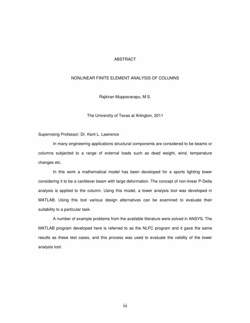
ABSTRACT
NONLINEAR FINITE ELEMENT ANALYSIS OF COLUMNS
Rajkiran Muppavarapu, M.S.
The University of Texas at Arlington, 2011
Supervising Professor: Dr. Kent L. Lawrence
In many engineering applications structural components are considered to be beams or
columns subjected to a range of external loads such as dead weight, wind, temperature
changes etc.
In this work a mathematical model has been developed for a sports lighting tower
considering it to be a cantilever beam with large deformation. The concept of non-linear P-Delta
analysis is applied to the column. Using this model, a tower analysis tool was developed in
MATLAB. Using this tool various design alternatives can be examined to evaluate their
suitability to a particular task.
A number of example problems from the available literature were solved in ANSYS. The
MATLAB program developed here is referred to as the NLFC program and it gave the same
results as these test cases, and this process was used to evaluate the validity of the tower
analysis tool.
iv
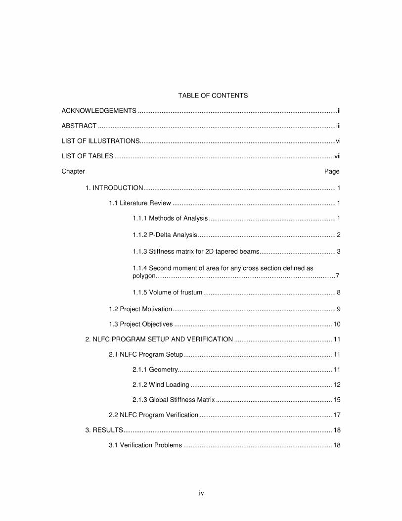
TABLE OF CONTENTS
ACKNOWLEDGEMENTS ..............................................................................................................ii
ABSTRACT ...................................................................................................................................iii
LIST OF ILLUSTRATIONS............................................................................................................vi
LIST OF TABLES .........................................................................................................................vii
Chapter Page
1. INTRODUCTION.......................................................................................................... 1
1.1 Literature Review .......................................................................................... 1
1.1.1 Methods of Analysis ...................................................................... 1
1.1.2 P-Delta Analysis............................................................................ 2
1.1.3 Stiffness matrix for 2D tapered beams.......................................... 3
1.1.4 Second moment of area for any cross section defined as polygon…………………………………………………..……….……..……7
1.1.5 Volume of frustum ......................................................................... 8
1.2 Project Motivation.......................................................................................... 9
1.3 Project Objectives ....................................................................................... 10
2. NLFC PROGRAM SETUP AND VERIFICATION ...................................................... 11
2.1 NLFC Program Setup.................................................................................. 11
2.1.1 Geometry..................................................................................... 11
2.1.2 Wind Loading .............................................................................. 12
2.1.3 Global Stiffness Matrix ................................................................ 15
2.2 NLFC Program Verification ......................................................................... 17
3. RESULTS................................................................................................................... 18
3.1 Verification Problems .................................................................................. 18
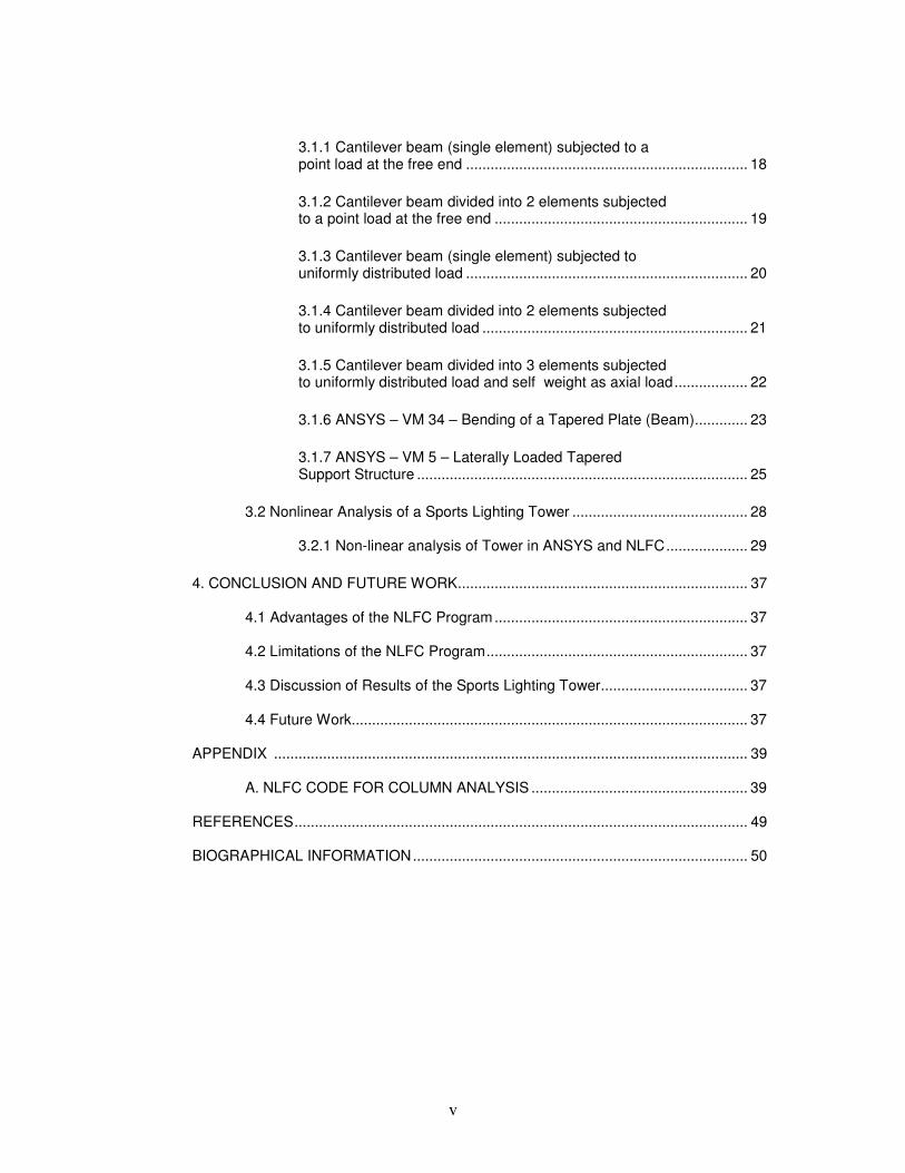
v
3.1.1 Cantilever beam (single element) subjected to a point load at the free end ..................................................................... 18
3.1.2 Cantilever beam divided into 2 elements subjected to a point load at the free end .............................................................. 19
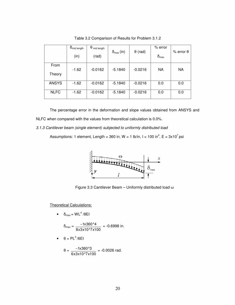
3.1.3 Cantilever beam (single element) subjected to uniformly distributed load ..................................................................... 20
3.1.4 Cantilever beam divided into 2 elements subjected to uniformly distributed load ................................................................. 21
3.1.5 Cantilever beam divided into 3 elements subjected to uniformly distributed load and self weight as axial load.................. 22
3.1.6 ANSYS – VM 34 – Bending of a Tapered Plate (Beam)............. 23
3.1.7 ANSYS – VM 5 – Laterally Loaded Tapered Support Structure ................................................................................. 25
3.2 Nonlinear Analysis of a Sports Lighting Tower ........................................... 28
3.2.1 Non-linear analysis of Tower in ANSYS and NLFC.................... 29
4. CONCLUSION AND FUTURE WORK....................................................................... 37
4.1 Advantages of the NLFC Program.............................................................. 37
4.2 Limitations of the NLFC Program................................................................ 37
4.3 Discussion of Results of the Sports Lighting Tower.................................... 37
4.4 Future Work................................................................................................. 37
APPENDIX .................................................................................................................... 39
A. NLFC CODE FOR COLUMN ANALYSIS ..................................................... 39
REFERENCES............................................................................................................... 49
BIOGRAPHICAL INFORMATION.................................................................................. 50
vi
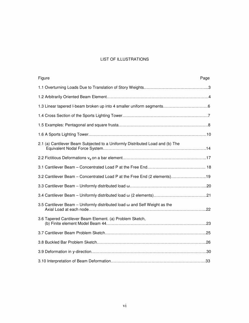
LIST OF ILLUSTRATIONS
Figure Page
1.1 Overturning Loads Due to Translation of Story Weights………………………………………...3
1.2 Arbitrarily Oriented Beam Element…………………………………………………………………4
1.3 Linear tapered I-beam broken up into 4 smaller uniform segments……………………………6
1.4 Cross Section of the Sports Lighting Tower………………………………………………………7
1.5 Examples: Pentagonal and square frusta…………………………………………………………8
1.6 A Sports Lighting Tower……………………………………………………………………………10
2.1 (a) Cantilever Beam Subjected to a Uniformly Distributed Load and (b) The Equivalent Nodal Force System………………………………………………………………….14
2.2 Fictitious Deformations νφ on a bar element……………………………………………………..17
3.1 Cantilever Beam – Concentrated Load P at the Free End……………………………………. 18
3.2 Cantilever Beam – Concentrated Load P at the Free End (2 elements)……………………..19
3.3 Cantilever Beam – Uniformly distributed load ω………………………………………………...20
3.4 Cantilever Beam – Uniformly distributed load ω (2 elements)…………………………………21
3.5 Cantilever Beam – Uniformly distributed load ω and Self Weight as the Axial Load at each node…………………………………………………………………………...22 3.6 Tapered Cantilever Beam Element. (a) Problem Sketch, (b) Finite element Model Beam 44………………………………………………………………..23 3.7 Cantilever Beam Problem Sketch………………………………………………………………...25
3.8 Buckled Bar Problem Sketch……………………………………………………………………...26
3.9 Deformation in y-direction………………………………………………………………………….30
3.10 Interpretation of Beam Deformation…………………………………………………………….33
vii
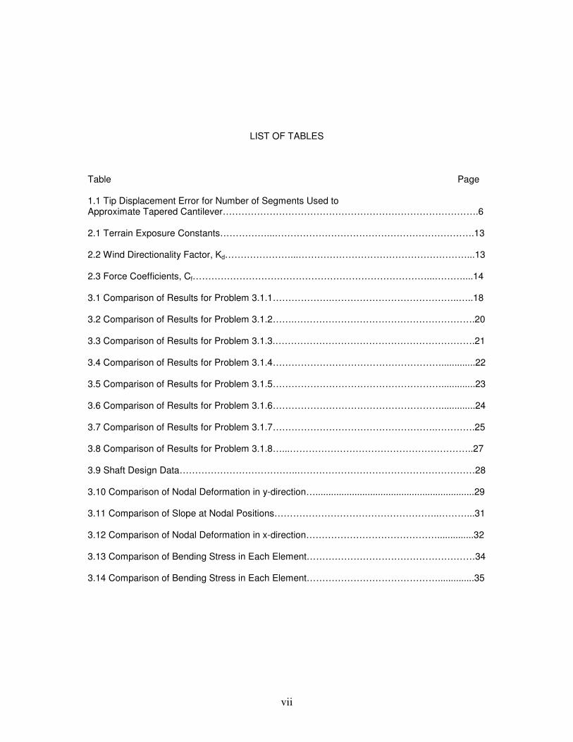
LIST OF TABLES
Table Page
1.1 Tip Displacement Error for Number of Segments Used to Approximate Tapered Cantilever……………………………………………………………………….6 2.1 Terrain Exposure Constants……………...……………………………………………………….13
2.2 Wind Directionality Factor, Kd…………………...………………………………………………...13
2.3 Force Coefficients, Cf…………………………………………………………………...………....14
3.1 Comparison of Results for Problem 3.1.1……………….…………………………………..…..18
3.2 Comparison of Results for Problem 3.1.2…….………………………………………………….20
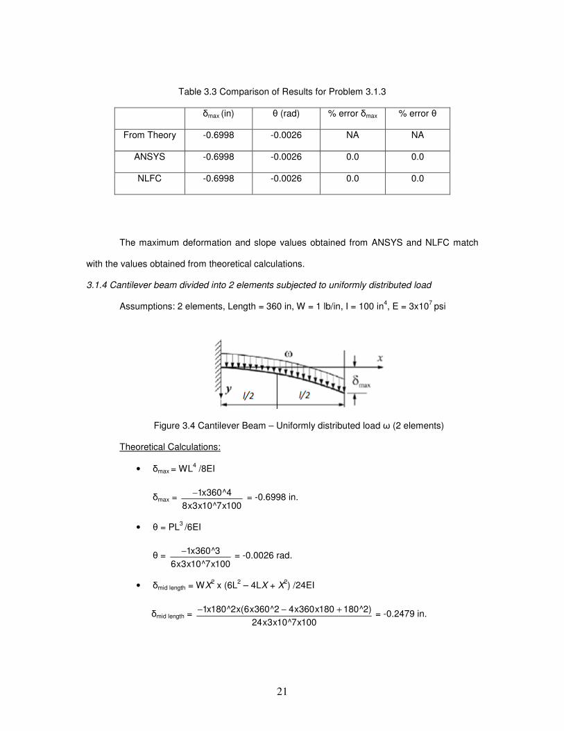
3.3 Comparison of Results for Problem 3.1.3.……………………………………………………….21
3.4 Comparison of Results for Problem 3.1.4……………………………………………….............22
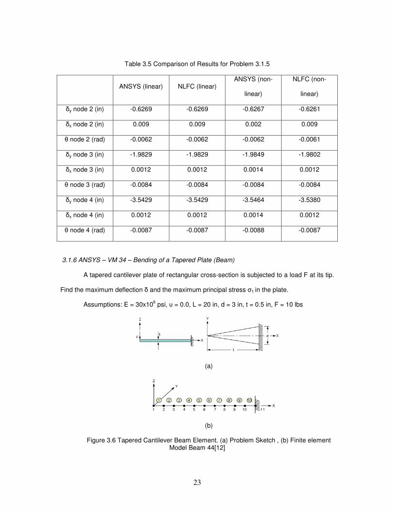
3.5 Comparison of Results for Problem 3.1.5……………………………………………….............23
3.6 Comparison of Results for Problem 3.1.6……………………………………………….............24
3.7 Comparison of Results for Problem 3.1.7…………………………………………….………….25
3.8 Comparison of Results for Problem 3.1.8…...…………………………………………………..27
3.9 Shaft Design Data………………………………..…………………………………………………28
3.10 Comparison of Nodal Deformation in y-direction….............................................................29
3.11 Comparison of Slope at Nodal Positions……………………………………………..………...31
3.12 Comparison of Nodal Deformation in x-direction……………………………………..............32
3.13 Comparison of Bending Stress in Each Element………………………………………………34
3.14 Comparison of Bending Stress in Each Element……………………………………..............35
1
CHAPTER 1
INTRODUCTION
Among the various numerical methods available, finite element method is very popular
and widely used. It is perhaps the most sophisticated tool for solving engineering problems.
When the structures have complicated shapes the conventional methods fail to give accurate
solutions and also it is quite uneconomical and time consuming. Almost any structure having
any shape and made of any material can be analyzed by the finite element method. Such an
advantage is not available with other methods.
Finite element analysis has now become an integral part of computer aided engineering
(CAE) and is being extensively used in the analysis and design of many complex real life
systems. While it started off as an extension of matrix methods of structural analysis it was
initially perceived as a tool for structural analysis alone, its applications now range from
structures to bio mechanics to electromagnetic field problems. Simple linear static problems as
well as highly complex nonlinear transient dynamic problems are effectively solved using the
finite element method. The field of finite element analysis has matured and now rests on
rigorous mathematical foundation. In preprocessing we build the model by defining geometry,
specifying element type, defining material properties, creating mesh, applying loading and
boundary conditions. In post processing we can extract results such as displacements, stresses
etc., time history relation wherever applicable and graphical representation of the results [1].
1.1 Literature Review
1.1.1 Methods of Analysis
Structural analysis can be divided into two groups, analytical methods and numerical
methods. Analytical methods cannot easily be used for complex structures and so numerical
methods must be used.
2
The numerical methods of structural analysis can be divided into two types: (1)
numerical solutions of differential equations for displacements and stresses and (2) matrix
methods based on discrete element idealization.[2]
In the first type, the equations of elasticity are solved for a given structural configuration
by using the finite difference techniques or by direct numerical integration. This method involves
mathematical approximation of differential equations.
The second method, matrix methods, is a concept that is used to replace the actual
continuous structure by a mathematical model made up of structural elements of finite size with
known elastic and inertial properties that can be expressed in matrix form.
In matrix methods, particles are of finite size and shape and are referred to as structural
elements. The analysis of the entire structure is done by analyzing the assembly of the
structural elements. When the size of these elements is decreased, the deformational behavior
of the mathematical model (under some restrictions) converges to that of the continuous
structure.
There are two types of matrix methods: (1) the displacement method (stiffness method),
where displacements are the unknowns, and (2) the force method (flexibility method), where
forces are unknowns. In both these methods the analysis can be considered as a combination
of individual unassembled structural elements into an assembled structure in which conditions
of equilibrium and compatibility are satisfied.
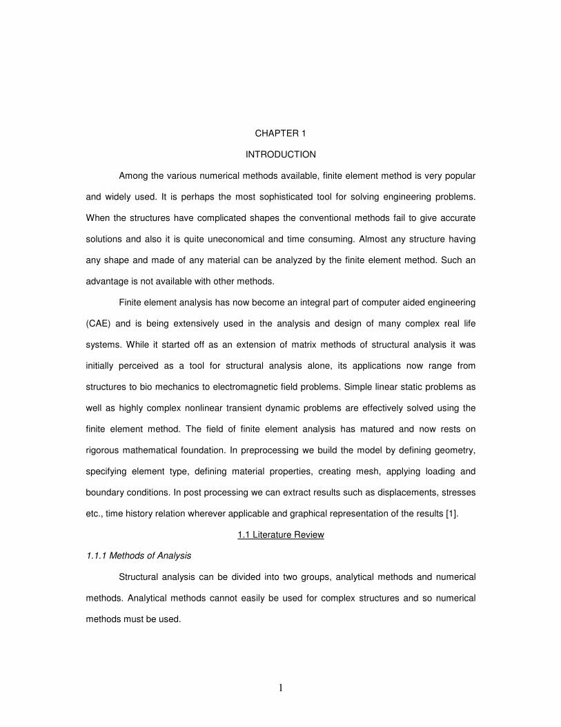
1.1.2 P-Delta Analysis
Using the geometric stiffness matrix is a method to include the secondary effects in the
static and dynamic analysis of all types of structural systems [3]. In civil structural engineering
this method is referred to as P-Delta analysis. This type of analysis is based on a more physical
approach. For example, in building analysis the lateral movement of a story mass to a deformed
position generates second-order overturning moments. This additional overturning moments on
the building are equal to the sum of the story weights ‘P’ times the lateral displacements ‘Delta’.
3
For structures where the weight is constant during lateral motions, the P-Delta problem
can be linearized. The solution is also obtained directly and exactly without iteration. This
method does not require iteration since the total axial force that is applied at each story level is
equal to the weight of the building above that level and it remains constant even when lateral
loads are applied.
Figure 1.1 Overturning Loads Due to Translation of Story Weights[8]
The vertical cantilever type structure shown in the Figure 1.1 best illustrates the basic
problem.
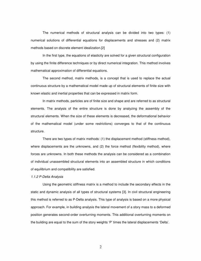
1.1.3 Stiffness matrix for 2D tapered beams
1.1.3.1 Two-dimensional Arbitrarily Oriented Beam Element Elastic Stiffness Matrix
The stiffness matrix for an arbitrarily oriented beam element, as shown in Figure 1.2, is
in a manner similar to that used for the bar element. The local axes ẋ and ẏ are located along
the beam element and transverse to the beam element, respectively, and the global axes x and
y are located to be convenient for the total structure.[4]
4
Figure 1.2 Arbitrarily Oriented Beam Element[4]
For a beam element the transformation matrix is defined as:
T =
−
−
100000
0CS000
000100
0000CS
(1.1)
The axial effects are not included yet. Here, C=cosθ and S=sinθ.
The global stiffness matrix for a beam element that includes shear and bending
resistance is as follows:
where
‘E’ is Young’s modulus,
‘I’ is principal moment of inertia about the z axis,
‘L’ length of the element,
5
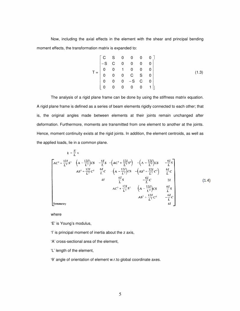
Now, including the axial effects in the element with the shear and principal bending
moment effects, the transformation matrix is expanded to:
T =
−
−
100000
0CS000
0SC000
000100
0000CS
0000SC
(1.3)
The analysis of a rigid plane frame can be done by using the stiffness matrix equation.
A rigid plane frame is defined as a series of beam elements rigidly connected to each other; that
is, the original angles made between elements at their joints remain unchanged after
deformation. Furthermore, moments are transmitted from one element to another at the joints.
Hence, moment continuity exists at the rigid joints. In addition, the element centroids, as well as
the applied loads, lie in a common plane.
where
‘E’ is Young’s modulus,
‘I’ is principal moment of inertia about the z axis,
‘A’ cross-sectional area of the element,
‘L’ length of the element,
‘θ’ angle of orientation of element w.r.to global coordinate axes.

6
Now to apply the above method of constructing stiffness matrix for a tapered beam
element; the element is broken down into smaller sections. The section properties for each of
these elements are taken from the point on the true tapered beam that corresponds to the
midpoint of a given piece.[5]
Figure 1.3 Linear tapered I-beam broken up into 4 smaller uniform segments[5]
Using this procedure the tip deflection results are compared to various cases with
number of segments ‘n’. The table 1.1 shows the convergence as the number of segments
increases.
Table 1.1 Tip displacement error for number of segments used to approximate tapered cantilever[5]
7
1.1.3.2 Geometrical Stiffness Matrix
The elastic stiffness matrix is calculated as shown in the previous section. When large
deflections are present, the equations of force equilibrium must be formulated for the deformed
configuration of the structure. This means that the linear relationship ‘F=KD’ between the
applied forces ‘F’ and the displacements ‘D’ cannot be used. However, because of the presence
of large deflections, strain-displacement equations contain nonlinear terms, which must be
included in calculating the stiffness matrix.[3]
K = KE + KG (1.5)
The geometric stiffness matrix is given by:
KG = Faxial/L
−
−−−
−
−
15/2^L210/L030/2^L10/L0
10/L5/6010/L5/60
000000
30/2^L10/L015/2^L210/L0
10/L5/6010/L5/60
000000
(1.6)
where
‘Faxial’ is the axial nodal force,
‘L’ is length of the element.
1.1.4 Second moment of area for any cross section defined as polygon
The second moment of are of a polygon can be calculated by adding up the individual
contributions of each segment of the polygon[6].
Figure 1.4 Cross Section of the Sports Lighting Tower
8
For this problem, each segment is a triangle. The number of triangles is equal to the
number of sides of the polygon. Two corners of each triangle segment are on the perimeter of
the polygon and the third corner is the origin of the polygon. The following are the equations to
calculate the second moments of area of the polygon:
Ix = 12
1∑
=
n
1i
( y2
i + yi yi+1 + y2
i+1) ai
Iy = 12
1∑
=
n
1i
( x2
i + xi xi+1 + x2
i+1) ai (1.7)
Ixy = 24
1∑
=
n
1i
( xi yi+1 + 2 xi yi + 2 xi+1 yi+1 + xi+1 yi) ai
• ai = xi yi+1 – xi+1 yi is twice the area of the elementary triangle,
• index ‘i' passes overall ‘n’ points in the polygon, which is considered closed, i.e. point
‘n+1’ is point 1.
According to these formulae the points defining the polygon are in anticlockwise order.
For a clockwise defined polygon these formulae will give negative values.
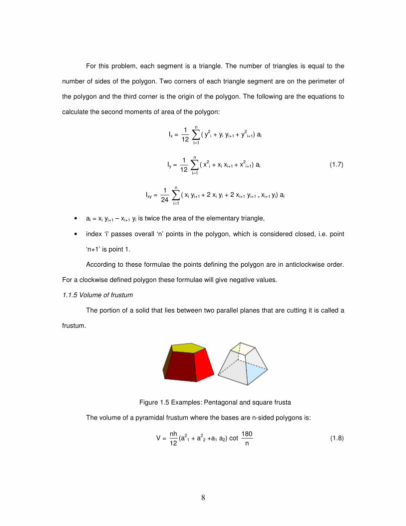
1.1.5 Volume of frustum
The portion of a solid that lies between two parallel planes that are cutting it is called a
frustum.
Figure 1.5 Examples: Pentagonal and square frusta
The volume of a pyramidal frustum where the bases are n-sided polygons is:
V = 12
nh(a
21 + a
22 +a1 a2) cot
n
180 (1.8)
9
where
‘a1’ and ‘a2’ are the sides of the bottom and top of the frustum respectively,
‘h’ is the height of the frustum.
1.2 Project Motivation
Light steel structures have been extensively used as being the most effective in
practical application. The main advantages of this kind of structures are the effective use of
materials and quick erection as well as their good characteristics. Over the past two decades,
solution of the buildings with tapered frames, manufactured from high tensile strength steel,
have become a standard. Their contours are quite close to the bending moment diagram, so the
cross-section is effectively utilized. Analysis of such kind of frames is rather complicated and not
widely investigated. This concept can be applied to a range of structures in various fields.[10]
The results of buckling analysis for a tapered column under the combination of an axial
force and a bending moment cannot be obtained just by adding the solutions obtained for those
loads acting separately because this dependency is non-linear.
A FEM stability analysis of tapered beam columns by Sapalas, Samofalov and
Saraskinas was done in 2004.[10] In this a theoretical and a numerical analysis of tapered
beam columns subjected to a bending moment and an axial force was conducted. Critical forces
were calculated by using a correction factor.
The analysis of tapered members are covered in many textbooks on structural analysis,
e.g., Przemieniecki.[2] The analysis involves lengthy calculations for each member. The
alternative is to use methods such as finite element method, where the member is represented
by a number of segments and the stiffness matrix for the segments are superimposed to
produce the stiffness matrix for the whole member. Because of current digital computer
capacities the increase in the number of equations due to the process of member discretization
is not disadvantageous. The disadvantage is the huge amount of input data required, especially
in the case of large structures.

10
1.3 Project Objectives
There are three main objectives in this project:
• To reduce the amount of input data required to analyze large structures.
• To reduce the number of steps in analyzing the structure.
• To develop a robust tool in MATLAB to analyze a large structure, by using the
methods mentioned above.
A sports lighting tower as shown in Figure 1.6, will be analyzed to find the deformations
and stresses under wind loading and self weight. The tower has polygonal cross section.
Figure 1.6 A Sports Lighting Tower[11]
The thesis will have the following sections:
• Chapter 2: NLFC Program Setup and Verification
• Chapter 3: Discussion of Results
• Chapter 4: Conclusion and Future Work
11
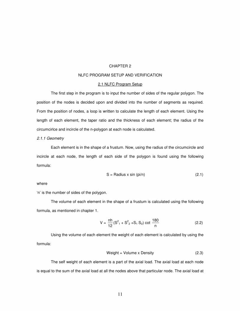
CHAPTER 2
NLFC PROGRAM SETUP AND VERIFICATION
2.1 NLFC Program Setup
The first step in the program is to input the number of sides of the regular polygon. The
position of the nodes is decided upon and divided into the number of segments as required.
From the position of nodes, a loop is written to calculate the length of each element. Using the
length of each element, the taper ratio and the thickness of each element; the radius of the
circumcirlce and incircle of the n-polygon at each node is calculated.
2.1.1 Geometry
Each element is in the shape of a frustum. Now, using the radius of the circumcircle and
incircle at each node, the length of each side of the polygon is found using the following
formula:
S = Radius x sin (pi/n) (2.1)
where
‘n’ is the number of sides of the polygon.
The volume of each element in the shape of a frustum is calculated using the following
formula, as mentioned in chapter 1.
V = 12
nh(S
21 + S
22 +S1 S2) cot
n
180 (2.2)
Using the volume of each element the weight of each element is calculated by using the
formula:
Weight = Volume x Density (2.3)
The self weight of each element is a part of the axial load. The axial load at each node
is equal to the sum of the axial load at all the nodes above that particular node. The axial load at
12
the nodes due to structural parts such as light fixtures etc., of the actual structure is also added
to this.
Next the second moment of area at each node with respect to different axes is
calculated according to section 1.1.4 of Chapter 1. For this, the coordinates of the polygon at
each node are to be calculated. This is done generating a polygon in MATLAB by using the
radius of the circumcircle and limiting the number of points to the number of sides of the
polygon. The following command is used to generate the circle:
t = linspace (0,2*pi,n+1) (2.4)
Then each coordinate is calculated using the angle at which each point was used to
make the circle, using the following formula:
X = Radius x sin (t)
Y = Radius x cosine (t) (2.5)
A total of ‘n+1’ sets of coordinates are generated but the first set of coordinates is the
same as the ‘n+1’th set.
2.1.2 Wind Loading
The effect of wind forces on the structure is calculated. The wind forces are lateral
loads on the structure. The calculation of wind loads is done as per ASCE 7-02 code for
cantilevered structures classified as other structures.
There are various constants that need to be calculated to get the wind forces acting on
each element. The first is ‘Kz’, velocity pressure exposure coefficient at height ‘z’. the formula to
calculate ‘Kz’ is as follows:
If Z < 15 then: Kz = 2.01*(15/Zg) ^ (2/α)
If Z >= 15 then: Kz = 2.01*(Z/Zg) ^ (2/α) (2.6)
where ‘Z’ is the height of the element above the ground.
‘Zg’ and ‘α’ are called terrain exposure coefficients. These values can be obtained in Table 2.1.
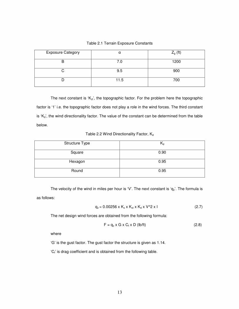
13
Table 2.1 Terrain Exposure Constants
Exposure Category α Zg (ft)
B 7.0 1200
C 9.5 900
D 11.5 700
The next constant is ‘Kzt’, the topographic factor. For the problem here the topographic
factor is ‘1’ i.e. the topographic factor does not play a role in the wind forces. The third constant
is ‘Kd’, the wind directionality factor. The value of the constant can be determined from the table
below.
Table 2.2 Wind Directionality Factor, Kd
Structure Type Kd
Square 0.90
Hexagon 0.95
Round 0.95
The velocity of the wind in miles per hour is ‘V’. The next constant is ‘qz’. The formula is
as follows:
qz = 0.00256 x Kz x Kzt x Kd x V^2 x I (2.7)
The net design wind forces are obtained from the following formula:
F = qz x G x Cf x D (lb/ft) (2.8)
where
‘G’ is the gust factor. The gust factor the structure is given as 1.14.
‘Cf’ is drag coefficient and is obtained from the following table.
14
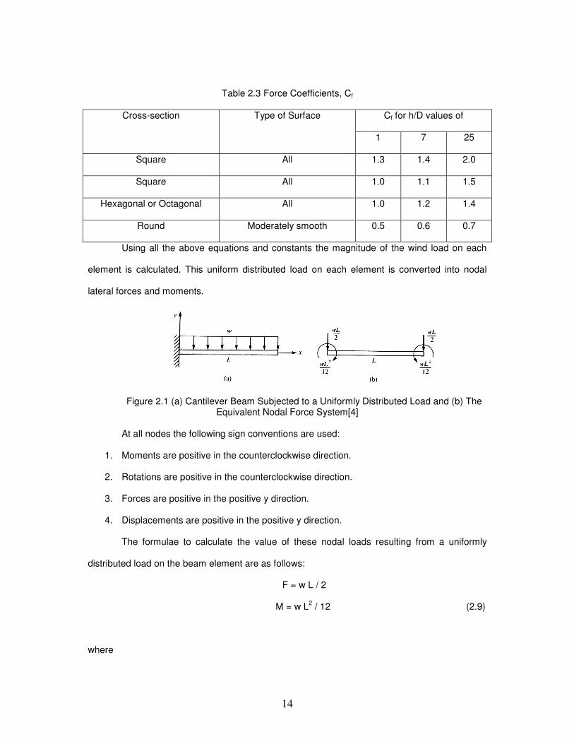
Table 2.3 Force Coefficients, Cf
Cf for h/D values of Cross-section Type of Surface
1 7 25
Square All 1.3 1.4 2.0
Square All 1.0 1.1 1.5
Hexagonal or Octagonal All 1.0 1.2 1.4
Round Moderately smooth 0.5 0.6 0.7
Using all the above equations and constants the magnitude of the wind load on each
element is calculated. This uniform distributed load on each element is converted into nodal
lateral forces and moments.
Figure 2.1 (a) Cantilever Beam Subjected to a Uniformly Distributed Load and (b) The Equivalent Nodal Force System[4]
At all nodes the following sign conventions are used:
1. Moments are positive in the counterclockwise direction.
2. Rotations are positive in the counterclockwise direction.
3. Forces are positive in the positive y direction.
4. Displacements are positive in the positive y direction.
The formulae to calculate the value of these nodal loads resulting from a uniformly
distributed load on the beam element are as follows:
F = w L / 2
M = w L2 / 12 (2.9)
where
15
‘w’ is the uniformly distributed load
‘L” is the length of the beam element.
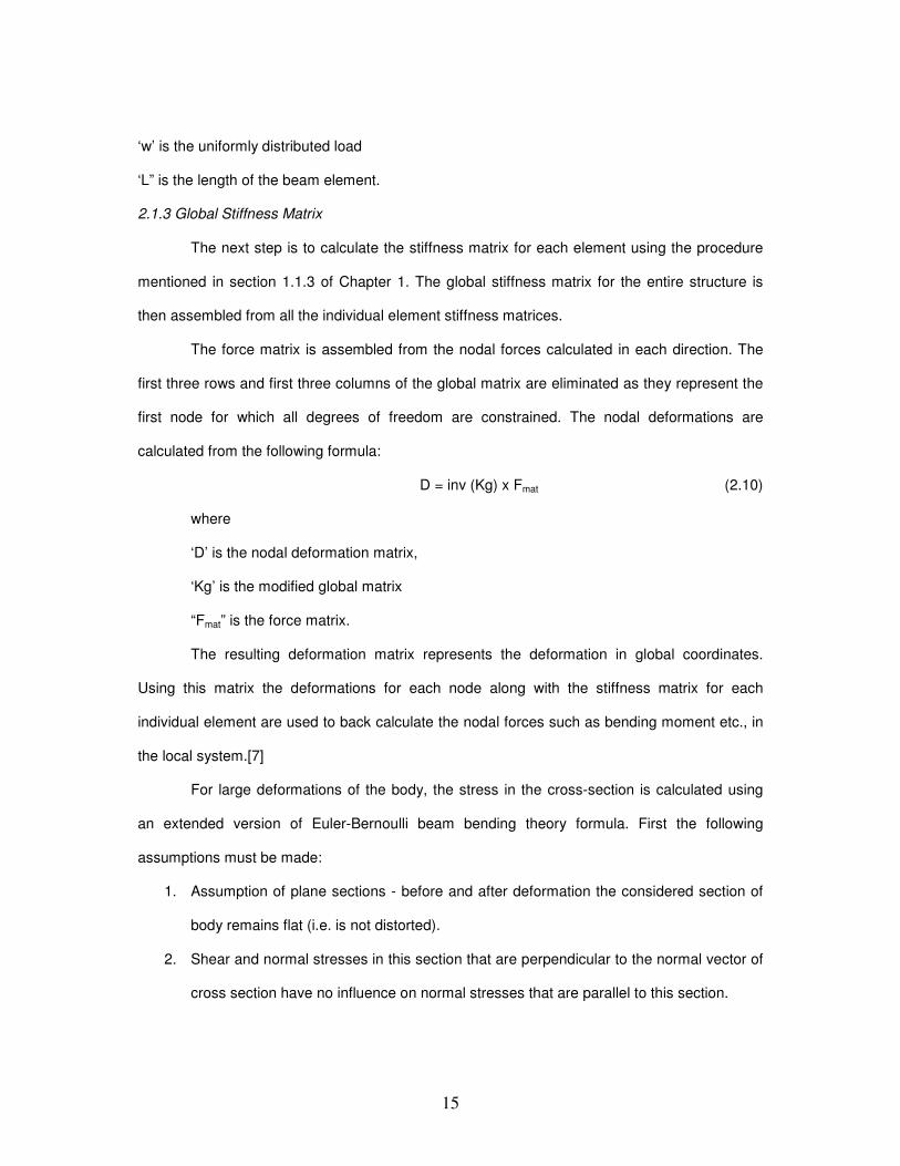
2.1.3 Global Stiffness Matrix
The next step is to calculate the stiffness matrix for each element using the procedure
mentioned in section 1.1.3 of Chapter 1. The global stiffness matrix for the entire structure is
then assembled from all the individual element stiffness matrices.
The force matrix is assembled from the nodal forces calculated in each direction. The
first three rows and first three columns of the global matrix are eliminated as they represent the
first node for which all degrees of freedom are constrained. The nodal deformations are
calculated from the following formula:
D = inv (Kg) x Fmat (2.10)
where
‘D’ is the nodal deformation matrix,
‘Kg’ is the modified global matrix
“Fmat” is the force matrix.
The resulting deformation matrix represents the deformation in global coordinates.
Using this matrix the deformations for each node along with the stiffness matrix for each
individual element are used to back calculate the nodal forces such as bending moment etc., in
the local system.[7]
For large deformations of the body, the stress in the cross-section is calculated using
an extended version of Euler-Bernoulli beam bending theory formula. First the following
assumptions must be made:
1. Assumption of plane sections - before and after deformation the considered section of
body remains flat (i.e. is not distorted).
2. Shear and normal stresses in this section that are perpendicular to the normal vector of
cross section have no influence on normal stresses that are parallel to this section.
16
Large bending considerations should be implemented when the bending radius ρ is
smaller than ten section heights h:
ρ < 10h
With those assumptions the stress in large bending is calculated as:
σ = A
Faxial +
A
M
ρ +
Ix'
My
y+ρ
ρ (2.11)
where
‘Faxial’ is the normal force
‘A’ is the section area
‘M’ is the bending moment
‘ρ’ is the local bending radius (the radius of bending at the current section)
Ix' is the area moment of inertia along the x axis, at the y place
‘y’ is the position along y axis on the section area in which the stress σ is calculated
When bending radius ρ approaches infinity and y is near zero, the original formula is
back:
σ = A
Faxial +
I
My (2.12)
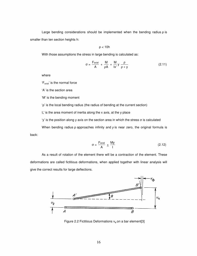
As a result of rotation of the element there will be a contraction of the element. These
deformations are called fictitious deformations, when applied together with linear analysis will
give the correct results for large deflections.
Figure 2.2 Fictitious Deformations νφ on a bar element[3]

17
The formula to calculate fictitious deformation is:
νφ = l2
1−(u4 – u2)
2 (2.13)
2.2 NLFC Program Verification
A series of simple example problems based on a cantilever beam were created. The
solutions were obtained by theoretical calculations. The problems were solved using the NLFC
program. The example problems were also solved using ANSYS. The results obtained from the
program and ANSYS were compared to the results from theoretical calculations. The different
example problems are as follows:
1. Cantilever beam (single element) subjected to a point load at the free end.
2. Cantilever beam divided into 2 elements subjected to a point load at the free end.
3. Cantilever beam (single element) subjected to uniformly distributed load.
4. Cantilever beam divided into 2 elements subjected to uniformly distributed load.
5. Cantilever beam divided into 3 elements subjected to uniformly distributed load and self
weight.
6. ANSYS – VM 34 – Bending of a Tapered Plate (Beam)
7. ANSYS – VM 5 – Laterally Loaded Tapered Support Structure.
8. ANSYS – VM 136 – Large Deflection of a Buckled Bar.
18
CHAPTER 3
RESULTS
3.1 Verification Problems
For the verification problems 3.1.1, 3.1.2, 3.1.3, 3.1.4 and 3.1.5 all the data was chosen
arbitrarily.
3.1.1 Cantilever beam (single element) subjected to a point load at the free end
Assumptions: 1 element, Length = 360 in, P = 1000 lb, I = 100 in4, E = 3x10
7 psi
Figure 3.1 Cantilever Beam – Concentrated Load P at the Free End
Theoretical Calculations:
• δmax = PL3 /3EI
δmax =
100x7^10x3x3
3^360x1000− = -5.1840 in.
• θ = PL2 /2EI
θ = 100x7^10x3x2
2^360x1000− = -0.0216 rad.
Table 3.1 Comparison of Results for Problem 3.1.1
δmax (in) θ (rad) % error δmax % error θ
From Theory -5.1840 -0.0216 NA NA
ANSYS -5.1840 -0.0216 0.0 0.0
NLFC -5.1840 -0.0216 0.0 0.0
19
The maximum deformation and slope values obtained from ANSYS and NLFC match
with the values obtained from theoretical calculations.
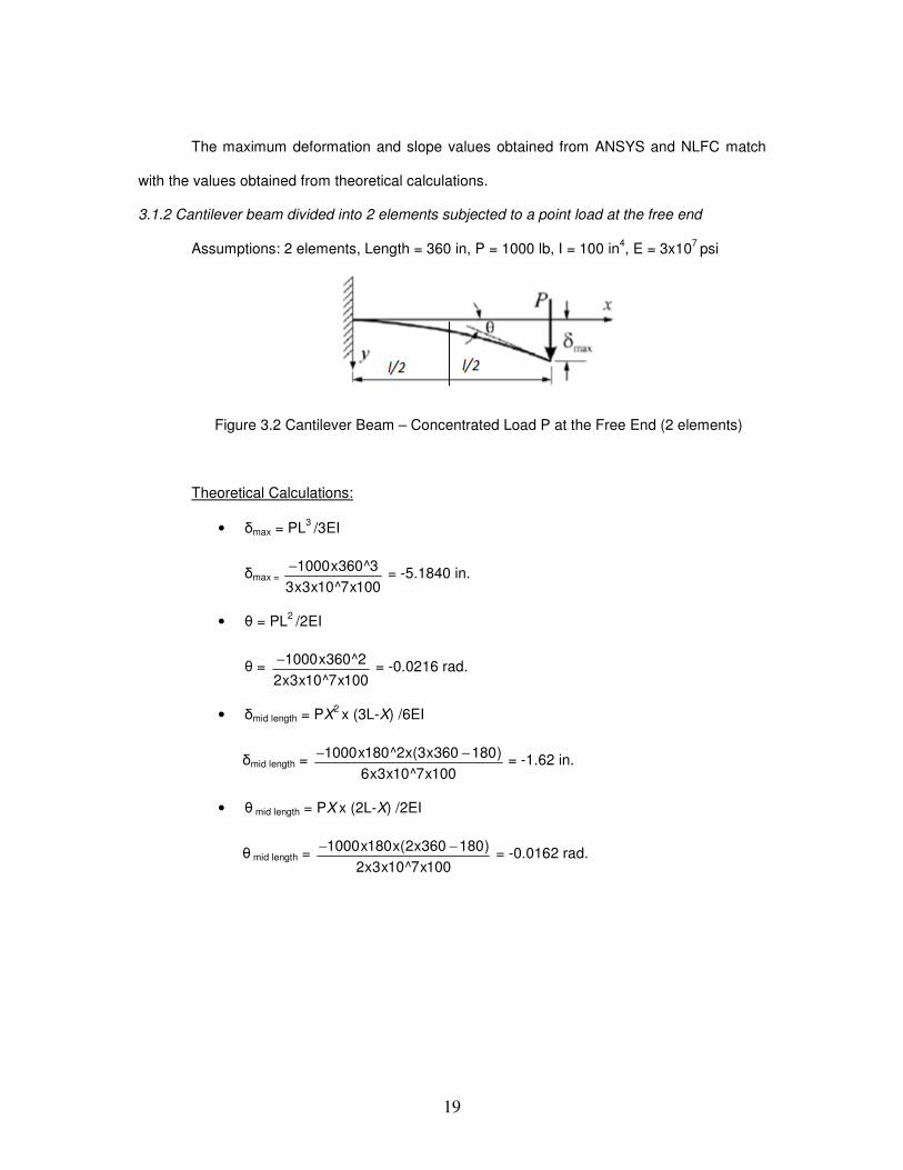
3.1.2 Cantilever beam divided into 2 elements subjected to a point load at the free end
Assumptions: 2 elements, Length = 360 in, P = 1000 lb, I = 100 in4, E = 3x10
7 psi
Figure 3.2 Cantilever Beam – Concentrated Load P at the Free End (2 elements)
Theoretical Calculations:
• δmax = PL3 /3EI
δmax =
100x7^10x3x3
3^360x1000− = -5.1840 in.
• θ = PL2 /2EI
θ = 100x7^10x3x2
2^360x1000− = -0.0216 rad.
• δmid length = PX2 x (3L-X) /6EI
δmid length = 100x7^10x3x6
)180360x3(x2^180x1000 −− = -1.62 in.
• θ mid length = PX x (2L-X) /2EI
θ mid length = 100x7^10x3x2
)180360x2(x180x1000 −− = -0.0162 rad.
20
Table 3.2 Comparison of Results for Problem 3.1.2
δmid length
(in)
θ mid length
(rad) δmax (in) θ (rad)
% error
δmax % error θ
From
Theory -1.62 -0.0162 -5.1840 -0.0216 NA NA
ANSYS -1.62 -0.0162 -5.1840 -0.0216 0.0 0.0
NLFC -1.62 -0.0162 -5.1840 -0.0216 0.0 0.0
The percentage error in the deformation and slope values obtained from ANSYS and
NLFC when compared with the values from theoretical calculation is 0.0%.
3.1.3 Cantilever beam (single element) subjected to uniformly distributed load
Assumptions: 1 element, Length = 360 in, W = 1 lb/in, I = 100 in4, E = 3x10
7 psi
Figure 3.3 Cantilever Beam – Uniformly distributed load ω
Theoretical Calculations:
• δmax = WL4 /8EI
δmax = 100x7^10x3x8
4^360x1− = -0.6998 in.
• θ = PL3 /6EI
θ = 100x7^10x3x6
3^360x1− = -0.0026 rad.
21
Table 3.3 Comparison of Results for Problem 3.1.3
δmax (in) θ (rad) % error δmax % error θ
From Theory -0.6998 -0.0026 NA NA
ANSYS -0.6998 -0.0026 0.0 0.0
NLFC -0.6998 -0.0026 0.0 0.0
The maximum deformation and slope values obtained from ANSYS and NLFC match
with the values obtained from theoretical calculations.
3.1.4 Cantilever beam divided into 2 elements subjected to uniformly distributed load
Assumptions: 2 elements, Length = 360 in, W = 1 lb/in, I = 100 in4, E = 3x10
7 psi
Figure 3.4 Cantilever Beam – Uniformly distributed load ω (2 elements)
Theoretical Calculations:
• δmax = WL4 /8EI
δmax = 100x7^10x3x8
4^360x1− = -0.6998 in.
• θ = PL3 /6EI
θ = 100x7^10x3x6
3^360x1− = -0.0026 rad.
• δmid length = WX2 x (6L
2 – 4LX + X
2) /24EI
δmid length = 100x7^10x3x24
)2^180180x360x42^360x6(x2^180x1 +−− = -0.2479 in.
22
• θ mid length = WX x (3L2 – 3LX + X
2) /6EI
θ mid length = 100x7^10x3x6
)2^180180x360x32^360x3(x180x1 +−− = -0.0023 rad.
Table 3.4 Comparison of Results for Problem 3.1.4
δmid length
(in)
θ mid length
(rad) δmax (in) θ (rad)
% error
δmax
% error
θ
From
Theory -0.2479 -0.0023 -0.6998 -0.0026 NA NA
ANSYS -0.2479 -0.0023 -0.6998 -0.0026 0.0 0.0
NLFC -0.2479 -0.0023 -0.6998 -0.0026 0.0 0.0
The percentage error in the deformation and slope values obtained from ANSYS and
NLFC when compared with the values from theoretical calculation is 0.0%.
3.1.5 Cantilever beam divided into 3 elements subjected to uniformly distributed load and self
weight as axial load
Assumptions: 3 elements, L = 180 in, W = 1 lb/in, I = 100 in4, E = 3x10
7 psi
Figure 3.5 Cantilever Beam – Uniformly distributed load ω and Self Weight as the Axial Load at each node
Both linear and non-linear analysis was carried out in ANSYS and the NLFC program.
23
Table 3.5 Comparison of Results for Problem 3.1.5
ANSYS (linear) NLFC (linear) ANSYS (non-
linear)
NLFC (non-
linear)
δy node 2 (in) -0.6269 -0.6269 -0.6267 -0.6261
δx node 2 (in) 0.009 0.009 0.002 0.009
θ node 2 (rad) -0.0062 -0.0062 -0.0062 -0.0061
δy node 3 (in) -1.9829 -1.9829 -1.9849 -1.9802
δx node 3 (in) 0.0012 0.0012 0.0014 0.0012
θ node 3 (rad) -0.0084 -0.0084 -0.0084 -0.0084
δy node 4 (in) -3.5429 -3.5429 -3.5464 -3.5380
δx node 4 (in) 0.0012 0.0012 0.0014 0.0012
θ node 4 (rad) -0.0087 -0.0087 -0.0088 -0.0087
3.1.6 ANSYS – VM 34 – Bending of a Tapered Plate (Beam)
A tapered cantilever plate of rectangular cross-section is subjected to a load F at its tip.
Find the maximum deflection δ and the maximum principal stress σ1 in the plate.
Assumptions: E = 30x106 psi, υ = 0.0, L = 20 in, d = 3 in, t = 0.5 in, F = 10 lbs
(a)
(b)
Figure 3.6 Tapered Cantilever Beam Element. (a) Problem Sketch , (b) Finite element Model Beam 44[12]
24
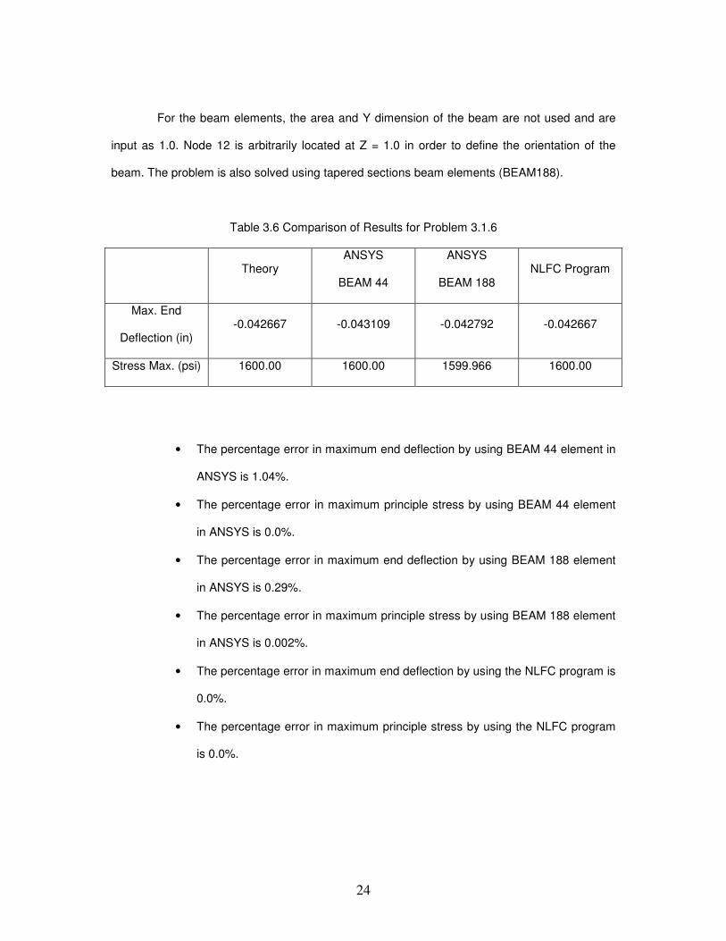
For the beam elements, the area and Y dimension of the beam are not used and are
input as 1.0. Node 12 is arbitrarily located at Z = 1.0 in order to define the orientation of the
beam. The problem is also solved using tapered sections beam elements (BEAM188).
Table 3.6 Comparison of Results for Problem 3.1.6
Theory ANSYS
BEAM 44
ANSYS
BEAM 188 NLFC Program
Max. End
Deflection (in) -0.042667 -0.043109 -0.042792 -0.042667
Stress Max. (psi) 1600.00 1600.00 1599.966 1600.00
• The percentage error in maximum end deflection by using BEAM 44 element in
ANSYS is 1.04%.
• The percentage error in maximum principle stress by using BEAM 44 element
in ANSYS is 0.0%.
• The percentage error in maximum end deflection by using BEAM 188 element
in ANSYS is 0.29%.
• The percentage error in maximum principle stress by using BEAM 188 element
in ANSYS is 0.002%.
• The percentage error in maximum end deflection by using the NLFC program is
0.0%.
• The percentage error in maximum principle stress by using the NLFC program
is 0.0%.
25
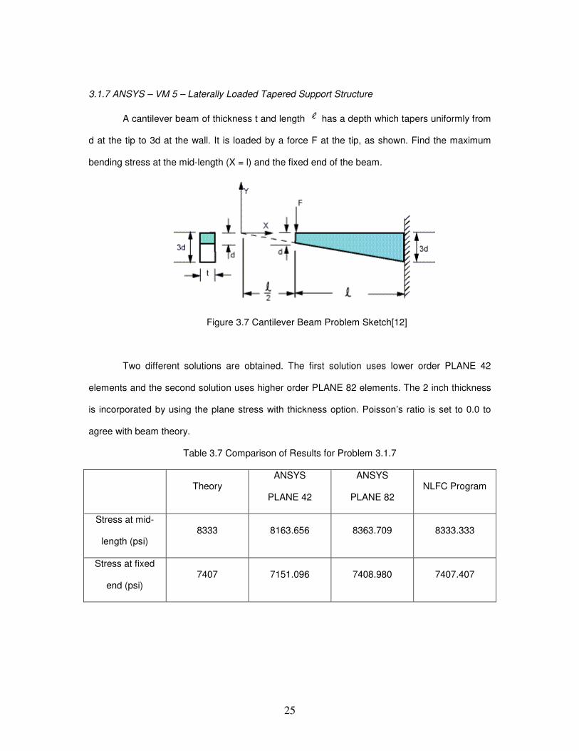
3.1.7 ANSYS – VM 5 – Laterally Loaded Tapered Support Structure
A cantilever beam of thickness t and length has a depth which tapers uniformly from
d at the tip to 3d at the wall. It is loaded by a force F at the tip, as shown. Find the maximum
bending stress at the mid-length (X = l) and the fixed end of the beam.
Figure 3.7 Cantilever Beam Problem Sketch[12]
Two different solutions are obtained. The first solution uses lower order PLANE 42
elements and the second solution uses higher order PLANE 82 elements. The 2 inch thickness
is incorporated by using the plane stress with thickness option. Poisson’s ratio is set to 0.0 to
agree with beam theory.
Table 3.7 Comparison of Results for Problem 3.1.7
Theory ANSYS
PLANE 42
ANSYS
PLANE 82 NLFC Program
Stress at mid-
length (psi) 8333 8163.656 8363.709 8333.333
Stress at fixed
end (psi) 7407 7151.096 7408.980 7407.407
26
• The percentage error in stress at mid length by using PLANE 42 element in
ANSYS is 2.03%.
• The percentage error in stress at fixed end by using PLANE 42 element in
ANSYS is 3.46%.
• The percentage error in stress at mid length by using PLANE 82 element in
ANSYS is 0.37%.
• The percentage error in stress at fixed end by using PLANE 42 element in
ANSYS is 0.03%.
• The percentage error in stress at mid length by using the NLFC program is
0.004%.
• The percentage error in stress at fixed end by using the NLFC program is
0.006%.
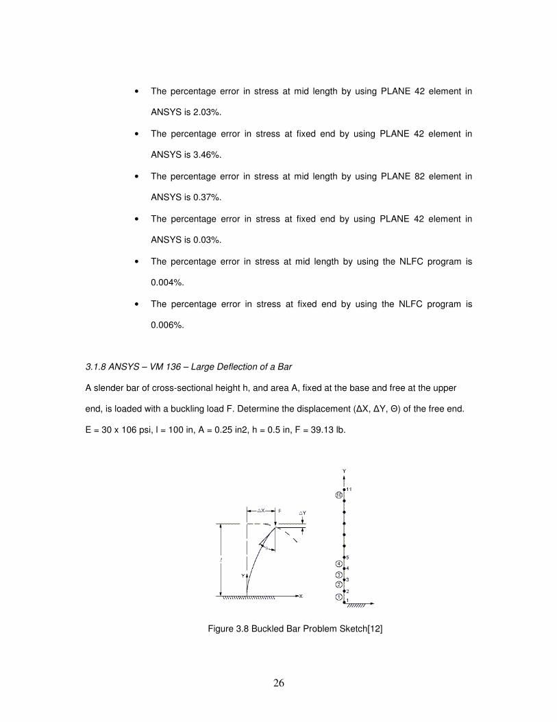
3.1.8 ANSYS – VM 136 – Large Deflection of a Bar
A slender bar of cross-sectional height h, and area A, fixed at the base and free at the upper
end, is loaded with a buckling load F. Determine the displacement (∆X, ∆Y, Θ) of the free end.
E = 30 x 106 psi, l = 100 in, A = 0.25 in2, h = 0.5 in, F = 39.13 lb.
Figure 3.8 Buckled Bar Problem Sketch[12]
27
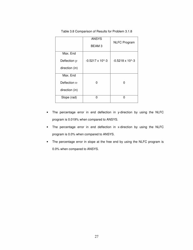
Table 3.8 Comparison of Results for Problem 3.1.8
ANSYS
BEAM 3 NLFC Program
Max. End
Deflection y-
direction (in)
-0.5217 x 10^-3 -0.5218 x 10^-3
Max. End
Deflection x-
direction (in)
0 0
Slope (rad) 0 0
• The percentage error in end deflection in y-direction by using the NLFC
program is 0.019% when compared to ANSYS.
• The percentage error in end deflection in x-direction by using the NLFC
program is 0.0% when compared to ANSYS.
• The percentage error in slope at the free end by using the NLFC program is
0.0% when compared to ANSYS.
28
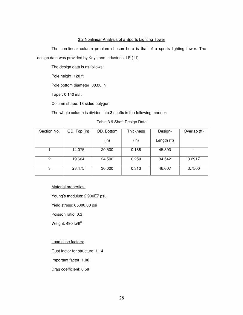
3.2 Nonlinear Analysis of a Sports Lighting Tower
The non-linear column problem chosen here is that of a sports lighting tower. The
design data was provided by Keystone Industries, LP.[11]
The design data is as follows:
Pole height: 120 ft
Pole bottom diameter: 30.00 in
Taper: 0.140 in/ft
Column shape: 18 sided polygon
The whole column is divided into 3 shafts in the following manner:
Table 3.9 Shaft Design Data
Section No. OD. Top (in) OD. Bottom
(in)
Thickness
(in)
Design-
Length (ft)
Overlap (ft)
1 14.075 20.500 0.188 45.893 -
2 19.664 24.500 0.250 34.542 3.2917
3 23.475 30.000 0.313 46.607 3.7500
Material properties:
Young’s modulus: 2.900E7 psi,
Yield stress: 65000.00 psi
Poisson ratio: 0.3
Weight: 490 lb/ft3
Load case factors:
Gust factor for structure: 1.14
Important factor: 1.00
Drag coefficient: 0.58
29
Direction of structure weight: X
Wind velocity in x-direction: 0.00 mph
Wind velocity in y-direction: 90.00 mph
Wind velocity in z-direction: 0.00 mph
There are other applied concentrated loads because of the light structures that are
applied at different nodes.
3.2.1 Non-linear analysis of Tower in ANSYS and NLFC
A Beam 3 element is used in ANSYS. The same problem is solved using the NLFC
code developed. These results are compared with the data provided by Keystone Industries,
LP.
Table 3.10 Comparison of Nodal Deformation in y-direction
Nodal Position (ft)
nodal deformation y-direction from given data
(in)
ANSYS nodal deformation
y-direction (in)
NLFC nodal deformation
y-direction (in)
0.0000 0.0000 0.0000 0.0000
5.0000 -0.1801 -0.1898 -0.1856
10.000 -0.7201 -0.76092 -0.7434
15.0000 -1.6255 -1.7219 -1.6817
20.0000 -2.9014 -3.0805 -3.0086
25.0000 -4.5528 -4.8434 -4.7321
30.0000 -6.5843 -7.0162 -6.86
35.0000 -8.9999 -9.6033 -9.3992
42.8570 -13.5782 -14.364 -14.085
46.6070 -16.0582 -16.87 -16.559
50.0000 -18.467 -19.264 -18.9284
55.0000 -22.3998 -23.143 -22.7784
60.0000 -26.785 -27.505 -27.1277
65.0000 -31.6184 -32.342 -31.9738
70.0000 -36.8926 -37.646 -37.3106
74.1070 -41.5459 -42.299 -42.007
77.3990 -45.4472 -46.164 -45.9178
80.0000 -48.6456 -49.3 -49.0972
85.0000 -55.1713 -55.664 -55.5618
90.0000 -62.1574 -62.496 -62.5257
95.0000 -69.5533 -69.742 -69.9392
100.000 -77.2937 -77.335 -77.738
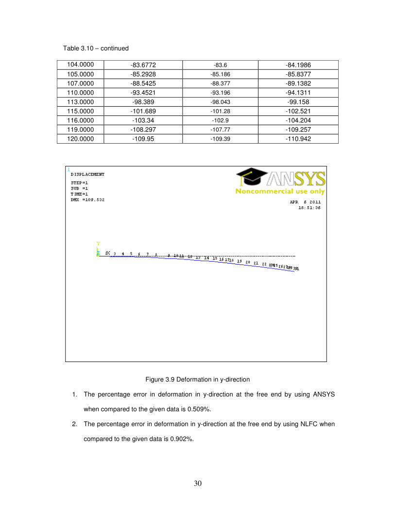
30
104.0000 -83.6772 -83.6 -84.1986
105.0000 -85.2928 -85.186 -85.8377
107.0000 -88.5425 -88.377 -89.1382
110.0000 -93.4521 -93.196 -94.1311
113.0000 -98.389 -98.043 -99.158
115.0000 -101.689 -101.28 -102.521
116.0000 -103.34 -102.9 -104.204
119.0000 -108.297 -107.77 -109.257
120.0000 -109.95 -109.39 -110.942
Figure 3.9 Deformation in y-direction
1. The percentage error in deformation in y-direction at the free end by using ANSYS
when compared to the given data is 0.509%.
2. The percentage error in deformation in y-direction at the free end by using NLFC when
compared to the given data is 0.902%.
Table 3.10 – continued
31
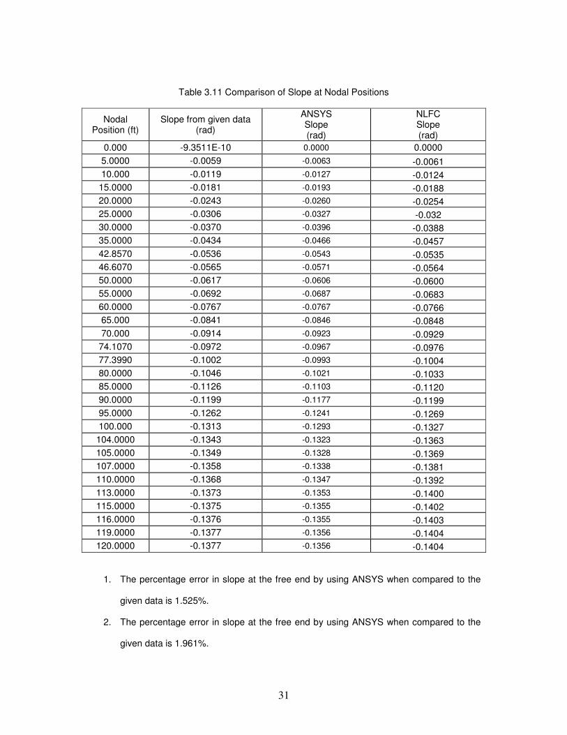
Table 3.11 Comparison of Slope at Nodal Positions
Nodal Position (ft)
Slope from given data (rad)
ANSYS Slope (rad)
NLFC Slope (rad)
0.000 -9.3511E-10 0.0000 0.0000
5.0000 -0.0059 -0.0063 -0.0061
10.000 -0.0119 -0.0127 -0.0124
15.0000 -0.0181 -0.0193 -0.0188
20.0000 -0.0243 -0.0260 -0.0254
25.0000 -0.0306 -0.0327 -0.032
30.0000 -0.0370 -0.0396 -0.0388
35.0000 -0.0434 -0.0466 -0.0457
42.8570 -0.0536 -0.0543 -0.0535
46.6070 -0.0565 -0.0571 -0.0564
50.0000 -0.0617 -0.0606 -0.0600
55.0000 -0.0692 -0.0687 -0.0683
60.0000 -0.0767 -0.0767 -0.0766
65.000 -0.0841 -0.0846 -0.0848
70.000 -0.0914 -0.0923 -0.0929
74.1070 -0.0972 -0.0967 -0.0976
77.3990 -0.1002 -0.0993 -0.1004
80.0000 -0.1046 -0.1021 -0.1033
85.0000 -0.1126 -0.1103 -0.1120
90.0000 -0.1199 -0.1177 -0.1199
95.0000 -0.1262 -0.1241 -0.1269
100.000 -0.1313 -0.1293 -0.1327
104.0000 -0.1343 -0.1323 -0.1363
105.0000 -0.1349 -0.1328 -0.1369
107.0000 -0.1358 -0.1338 -0.1381
110.0000 -0.1368 -0.1347 -0.1392
113.0000 -0.1373 -0.1353 -0.1400
115.0000 -0.1375 -0.1355 -0.1402
116.0000 -0.1376 -0.1355 -0.1403
119.0000 -0.1377 -0.1356 -0.1404
120.0000 -0.1377 -0.1356 -0.1404
1. The percentage error in slope at the free end by using ANSYS when compared to the
given data is 1.525%.
2. The percentage error in slope at the free end by using ANSYS when compared to the
given data is 1.961%.
32
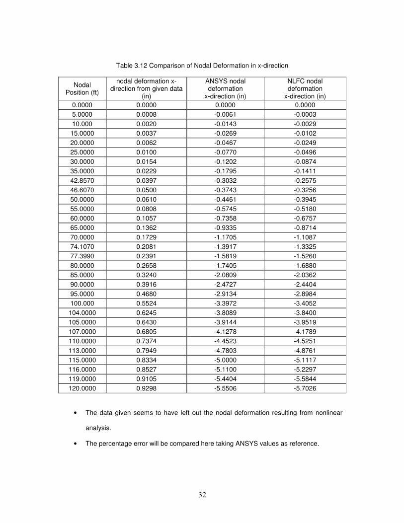
Table 3.12 Comparison of Nodal Deformation in x-direction
Nodal Position (ft)
nodal deformation x-direction from given data
(in)
ANSYS nodal deformation
x-direction (in)
NLFC nodal deformation
x-direction (in)
0.0000 0.0000 0.0000 0.0000
5.0000 0.0008 -0.0061 -0.0003
10.000 0.0020 -0.0143 -0.0029
15.0000 0.0037 -0.0269 -0.0102
20.0000 0.0062 -0.0467 -0.0249
25.0000 0.0100 -0.0770 -0.0496
30.0000 0.0154 -0.1202 -0.0874
35.0000 0.0229 -0.1795 -0.1411
42.8570 0.0397 -0.3032 -0.2575
46.6070 0.0500 -0.3743 -0.3256
50.0000 0.0610 -0.4461 -0.3945
55.0000 0.0808 -0.5745 -0.5180
60.0000 0.1057 -0.7358 -0.6757
65.0000 0.1362 -0.9335 -0.8714
70.0000 0.1729 -1.1705 -1.1087
74.1070 0.2081 -1.3917 -1.3325
77.3990 0.2391 -1.5819 -1.5260
80.0000 0.2658 -1.7405 -1.6880
85.0000 0.3240 -2.0809 -2.0362
90.0000 0.3916 -2.4727 -2.4404
95.0000 0.4680 -2.9134 -2.8984
100.000 0.5524 -3.3972 -3.4052
104.0000 0.6245 -3.8089 -3.8400
105.0000 0.6430 -3.9144 -3.9519
107.0000 0.6805 -4.1278 -4.1789
110.0000 0.7374 -4.4523 -4.5251
113.0000 0.7949 -4.7803 -4.8761
115.0000 0.8334 -5.0000 -5.1117
116.0000 0.8527 -5.1100 -5.2297
119.0000 0.9105 -5.4404 -5.5844
120.0000 0.9298 -5.5506 -5.7026
• The data given seems to have left out the nodal deformation resulting from nonlinear
analysis.
• The percentage error will be compared here taking ANSYS values as reference.
33
• The percentage error in deformation in x-direction at the free end by using the NLFC
program is 2.74%.
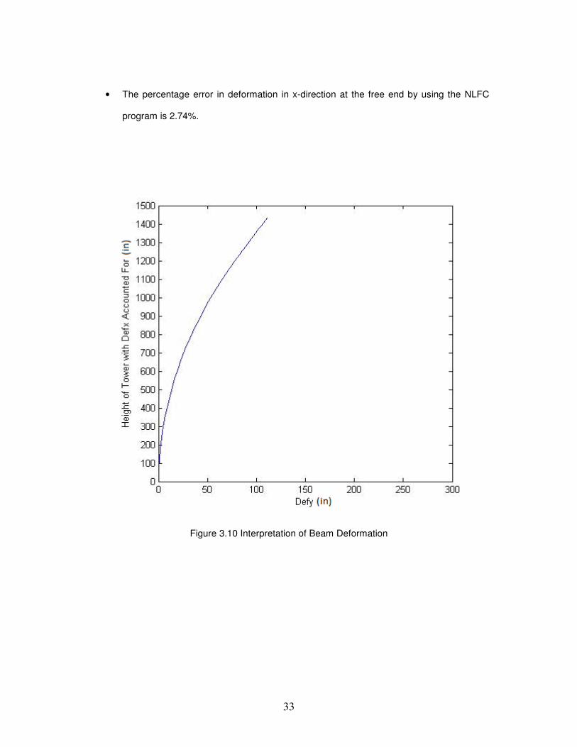
Figure 3.10 Interpretation of Beam Deformation
34
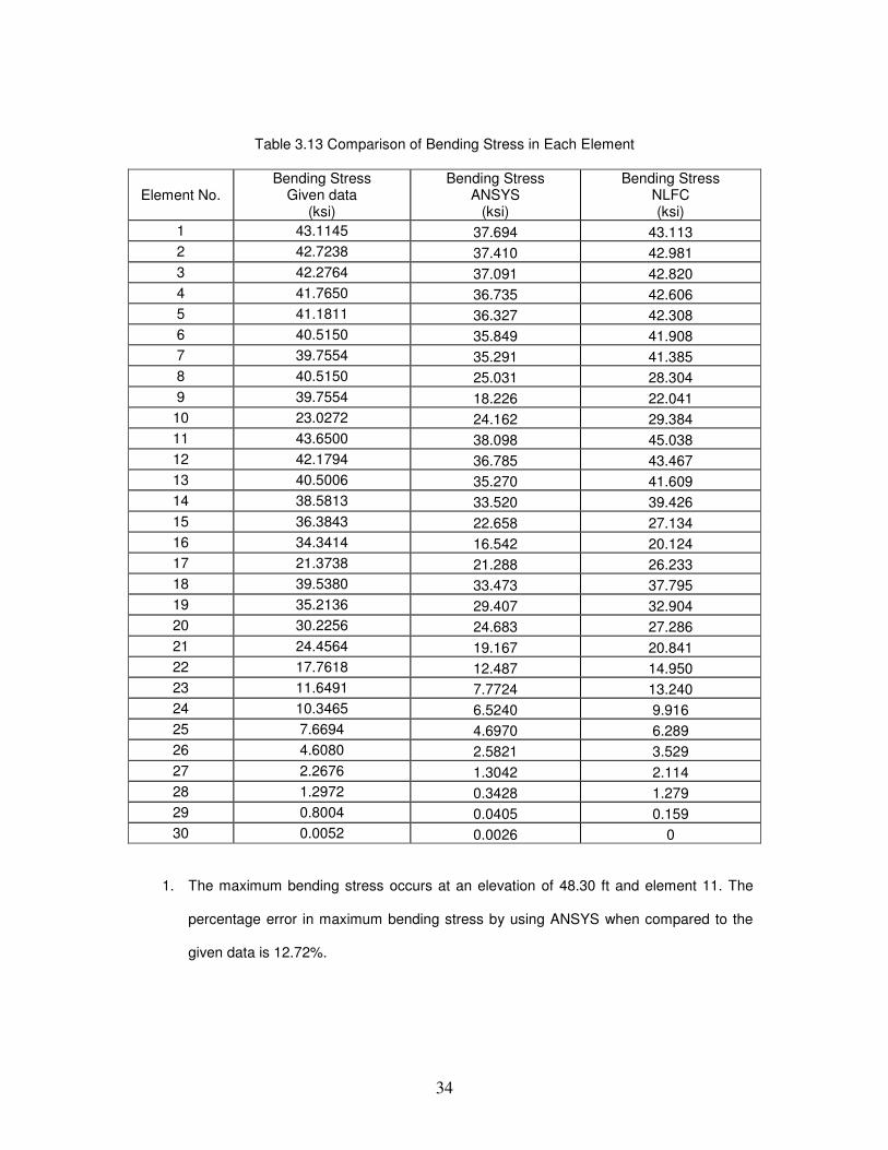
Table 3.13 Comparison of Bending Stress in Each Element
Element No. Bending Stress
Given data (ksi)
Bending Stress ANSYS
(ksi)
Bending Stress NLFC (ksi)
1 43.1145 37.694 43.113
2 42.7238 37.410 42.981
3 42.2764 37.091 42.820
4 41.7650 36.735 42.606
5 41.1811 36.327 42.308
6 40.5150 35.849 41.908
7 39.7554 35.291 41.385
8 40.5150 25.031 28.304
9 39.7554 18.226 22.041
10 23.0272 24.162 29.384
11 43.6500 38.098 45.038
12 42.1794 36.785 43.467
13 40.5006 35.270 41.609
14 38.5813 33.520 39.426
15 36.3843 22.658 27.134
16 34.3414 16.542 20.124
17 21.3738 21.288 26.233
18 39.5380 33.473 37.795
19 35.2136 29.407 32.904
20 30.2256 24.683 27.286
21 24.4564 19.167 20.841
22 17.7618 12.487 14.950
23 11.6491 7.7724 13.240
24 10.3465 6.5240 9.916
25 7.6694 4.6970 6.289
26 4.6080 2.5821 3.529
27 2.2676 1.3042 2.114
28 1.2972 0.3428 1.279
29 0.8004 0.0405 0.159
30 0.0052 0.0026 0
1. The maximum bending stress occurs at an elevation of 48.30 ft and element 11. The
percentage error in maximum bending stress by using ANSYS when compared to the
given data is 12.72%.
35
2. The maximum bending stress occurs at an elevation of 48.30 ft and element 11. The
percentage error in maximum bending stress by using NLFC when compared to the
given data is 3.18%.
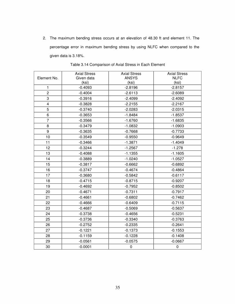
Table 3.14 Comparison of Axial Stress in Each Element
Element No. Axial Stress Given data
(ksi)
Axial Stress ANSYS
(ksi)
Axial Stress NLFC (ksi)
1 -0.4093 -2.8196 -2.8157
2 -0.4004 -2.6113 -2.6089
3 -0.3916 -2.4099 -2.4092
4 -0.3828 -2.2155 -2.2167
5 -0.3740 -2.0283 -2.0315
6 -0.3653 -1.8484 -1.8537
7 -0.3566 -1.6760 -1.6835
8 -0.3479 -1.0832 -1.0903
9 -0.3635 -0.7668 -0.7733
10 -0.3549 -0.9550 -0.9649
11 -0.3466 -1.3871 -1.4049
12 -0.3244 -1.2567 -1.278
13 -0.4088 -1.1355 -1.1605
14 -0.3889 -1.0240 -1.0527
15 -0.3817 -0.6662 -0.6892
16 -0.3747 -0.4674 -0.4864
17 -0.3680 -0.5842 -0.6117
18 -0.4715 -0.8715 -0.9207
19 -0.4692 -0.7952 -0.8502
20 -0.4671 -0.7311 -0.7917
21 -0.4661 -0.6802 -0.7462
22 -0.4666 -0.6409 -0.7115
23 -0.4687 -0.5069 -0.5637
24 -0.3738 -0.4656 -0.5231
25 -0.3736 -0.3340 -0.3763
26 -0.2752 -0.2335 -0.2641
27 -0.1221 -0.1373 -0.1553
28 -0.1159 -0.1228 -0.1408
29 -0.0561 -0.0575 -0.0667
30 -0.0001 0 0

36
1 The maximum axial stress is 2.8196 ksi and occurs in element 11 by using ANSYS.
2 The maximum axial stress is 2.8157 ksi and occurs in element 11 by using the NLFC
program.

37
CHAPTER 4
CONCLUSION AND FUTURE WORK
4.1 Advantages of the NLFC Program
The NLFC program is a very robust tool. This can be determined from the results and
comparisons shown in Chapter 3. The process of analyzing a column or beam like structure
from start to finish is faster than ANSYS, as all the calculations such as loads, moments etc. are
done within the program. The program can be easily modified to work with any kind of structure
such as an aeroplane wing, just by generating an aerofoil design instead of a regular polygon as
in the program.
4.2 Limitations of the NLFC Program
The NLFC program can be used for regular polygons only. The program uses the
concept of tapered beams by approximating the properties of each element to the properties of
the element at the geometrical centre. The program needs to be modified to analyze 3D
structures.
4.3 Discussion of Results of the Sports Lighting Tower
The NLFC program shows excellent agreement in deformation in y-direction, slope and
bending stresses with the data provided by Keystone Industries, LP. The most serious
disagreement with the given data comes in from deformation in x-direction results from ANSYS.
For nodal deformations in x-direction the data given seems to have left out the nodal
deformation resulting from nonlinear analysis.
4.4 Future Work
The results show that there are certain advantages to using the NLFC program.
However, these advantages can be increased and the errors reduced by implementing a 3

38
dimensional approach and also calculating the element properties along the length. The ability
to generate and analyse irregular polygons can also be considered.

39
APPENDIX A
NLFC CODE FOR COLUMN ANALYSIS
40
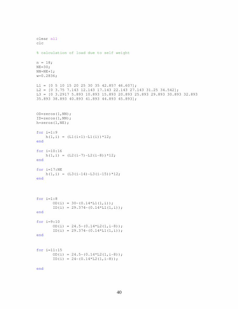
clear all clc
% calculation of load due to self weight
n = 18; NE=30; NN=NE+1; w=0.2836;
L1 = [0 5 10 15 20 25 30 35 42.857 46.607]; L2 = [0 3.75 7.143 12.143 17.143 22.143 27.143 31.25 34.542]; L3 = [0 3.2917 5.893 10.893 15.893 20.893 25.893 29.893 30.893 32.893
35.893 38.893 40.893 41.893 44.893 45.893];
OD=zeros(1,NN); ID=zeros(1,NN); h=zeros(1,NE);
for i=1:9 h(1,i) = (L1(i+1)-L1(i))*12; end
for i=10:16 h(1,i) = (L2(i-7)-L2(i-8))*12; end
for i=17:NE h(1,i) = (L3(i-14)-L3(i-15))*12; end
for i=1:8 OD(i) = 30-(0.14*L1(1,i)); ID(i) = 29.374-(0.14*L1(1,i)); end
for i=9:10 OD(i) = 24.5-(0.14*L2(1,i-8)); ID(i) = 29.374-(0.14*L1(1,i)); end
for i=11:15 OD(i) = 24.5-(0.14*L2(1,i-8)); ID(i) = 24-(0.14*L2(1,i-8));
end
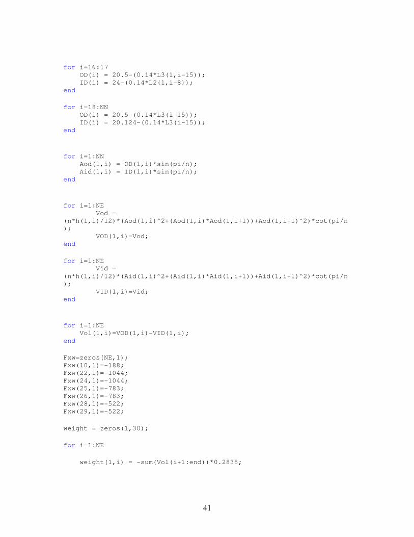
41
for i=16:17 OD(i) = 20.5-(0.14*L3(1,i-15)); ID(i) = 24-(0.14*L2(1,i-8)); end
for i=18:NN OD(i) = 20.5-(0.14*L3(i-15)); ID(i) = 20.124-(0.14*L3(i-15)); end
for i=1:NN Aod(1,i) = OD(1,i)*sin(pi/n); Aid(1,i) = ID(1,i)*sin(pi/n); end
for i=1:NE Vod =
(n*h(1,i)/12)*(Aod(1,i)^2+(Aod(1,i)*Aod(1,i+1))+Aod(1,i+1)^2)*cot(pi/n
); VOD(1,i)=Vod; end
for i=1:NE Vid =
(n*h(1,i)/12)*(Aid(1,i)^2+(Aid(1,i)*Aid(1,i+1))+Aid(1,i+1)^2)*cot(pi/n
); VID(1,i)=Vid; end
for i=1:NE Vol(1,i)=VOD(1,i)-VID(1,i); end
Fxw=zeros(NE,1); Fxw(10,1)=-188; Fxw(22,1)=-1044; Fxw(24,1)=-1044; Fxw(25,1)=-783; Fxw(26,1)=-783; Fxw(28,1)=-522; Fxw(29,1)=-522;
weight = zeros(1,30);
for i=1:NE
weight(1,i) = -sum(Vol(i+1:end))*0.2835;
42
end
Weight=weight'+Fxw;
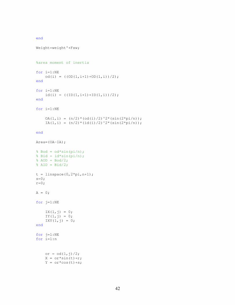
%area moment of inertia
for i=1:NE od(i) = ((OD(1,i+1)+OD(1,i))/2); end
for i=1:NE id(i) = ((ID(1,i+1)+ID(1,i))/2); end
for i=1:NE
OA(1,i) = (n/2)*(od(i)/2)^2*(sin(2*pi/n)); IA(1,i) = (n/2)*(id(i)/2)^2*(sin(2*pi/n));
end
Area=(OA-IA);
% Bod = od*sin(pi/n); % Bid = id*sin(pi/n); % AOD = Bod/2; % AID = Bid/2;
t = linspace(0,2*pi,n+1); s=0; r=0;
A = 0;
for j=1:NE
IX(1,j) = 0; IY(1,j) = 0; IXY(1,j) = 0; end
for j=1:NE for i=1:n
or = od(1,j)/2; X = or*sin(t)+r; Y = or*cos(t)+s;
43
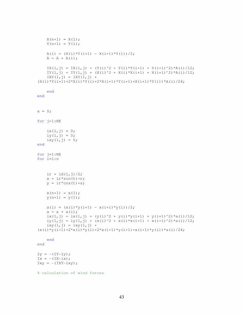
X(n+1) = X(1); Y(n+1) = Y(1);
A(i) = (X(i)*Y(i+1) - X(i+1)*Y(i))/2; A = A + A(i);
IX(1,j) = IX(1,j) + (Y(i)^2 + Y(i)*Y(i+1) + Y(i+1)^2)*A(i)/12; IY(1,j) = IY(1,j) + (X(i)^2 + X(i)*X(i+1) + X(i+1)^2)*A(i)/12; IXY(1,j) = IXY(1,j) +
(X(i)*Y(i+1)+2*X(i)*Y(i)+2*X(i+1)*Y(i+1)+X(i+1)*Y(i))*A(i)/24;
end end
a = 0;
for j=1:NE
ix(1,j) = 0; iy(1,j) = 0; ixy(1,j) = 0; end
for j=1:NE for i=1:n
ir = id(1,j)/2; x = ir*sin(t)+r; y = ir*cos(t)+s;
x(n+1) = x(1); y(n+1) = y(1);
a(i) = (x(i)*y(i+1) - x(i+1)*y(i))/2; a = a + a(i); ix(1,j) = ix(1,j) + (y(i)^2 + y(i)*y(i+1) + y(i+1)^2)*a(i)/12; iy(1,j) = iy(1,j) + (x(i)^2 + x(i)*x(i+1) + x(i+1)^2)*a(i)/12; ixy(1,j) = ixy(1,j) +
(x(i)*y(i+1)+2*x(i)*y(i)+2*x(i+1)*y(i+1)+x(i+1)*y(i))*a(i)/24;
end end
Iy = -(IY-iy); Ix = -(IX-ix); Ixy = -(IXY-ixy);
% calculation of wind forces
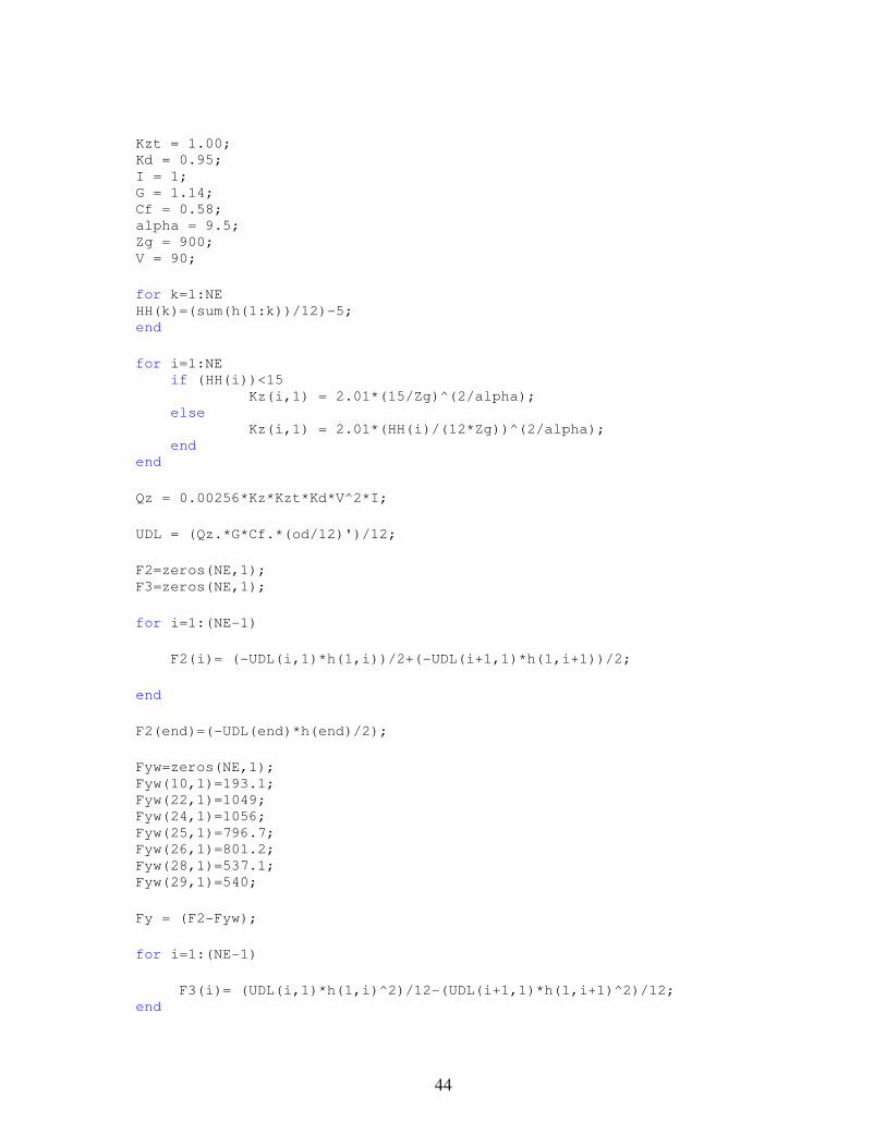
44
Kzt = 1.00; Kd = 0.95; I = 1; G = 1.14; Cf = 0.58; alpha = 9.5; Zg = 900; V = 90;
for k=1:NE HH(k)=(sum(h(1:k))/12)-5; end
for i=1:NE if (HH(i))<15 Kz(i,1) = 2.01*(15/Zg)^(2/alpha); else Kz(i,1) = 2.01*(HH(i)/(12*Zg))^(2/alpha); end end
Qz = 0.00256*Kz*Kzt*Kd*V^2*I;
UDL = (Qz.*G*Cf.*(od/12)')/12;
F2=zeros(NE,1); F3=zeros(NE,1);
for i=1:(NE-1)
F2(i)= (-UDL(i,1)*h(1,i))/2+(-UDL(i+1,1)*h(1,i+1))/2;
end
F2(end)=(-UDL(end)*h(end)/2);
Fyw=zeros(NE,1); Fyw(10,1)=193.1; Fyw(22,1)=1049; Fyw(24,1)=1056; Fyw(25,1)=796.7; Fyw(26,1)=801.2; Fyw(28,1)=537.1; Fyw(29,1)=540;
Fy = (F2-Fyw);
for i=1:(NE-1)
F3(i)= (UDL(i,1)*h(1,i)^2)/12-(UDL(i+1,1)*h(1,i+1)^2)/12; end
45
F3(end)=(UDL(end)*h(end)^2/12);
F=zeros(3*NE,1);
for i=1:3:3*NE for j=(i+2)/3
F(i)=Weight(j);
end end
for i=2:3:3*NE for j=(i+1)/3
F(i)=Fy(j);
end end
for i=3:3:3*NE for j=i/3
F(i)=F3(j);
end end
% calculation of element stifness matrix
E = 2.9e7; % deg = 0; % C = cos(deg*180/pi); % S = sin(deg*180/pi);
for i=1:NE
S(1,i)=((OD(1,i+1)/2)-(OD(1,i)/2))/(h(1,i)^2-((OD(1,i)/2)-
(OD(1,i+1)/2))^2)^0.5; C(1,i)=1-S(1,i)^2;
end
for i=1:NE
ke =
(E/h(1,i))*[(Area(1,i)*C(1,i)^2+12*(Iy(1,i)/h(1,i)^2)*S(1,i)^2)
(Area(1,i)-12*Iy(1,i)/h(1,i)^2)*C(1,i)*S(1,i) (-
6*Iy(1,i)/h(1,i))*S(1,i) -
46
(Area(1,i)*C(1,i)^2+12*(Iy(1,i)/h(1,i)^2)*S(1,i)^2) -(Area(1,i)-
12*Iy(1,i)/h(1,i)^2)*C(1,i)*S(1,i) (-6*Iy(1,i)/h(1,i))*S(1,i); (Area(1,i)-12*Iy(1,i)/h(1,i)^2)*C(1,i)*S(1,i)
(Area(1,i)*S(1,i)^2+12*(Iy(1,i)/h(1,i)^2)*C(1,i)^2)
(6*Iy(1,i)/h(1,i))*C(1,i) -(Area(1,i)-
12*Iy(1,i)/h(1,i)^2)*C(1,i)*S(1,i) -
(Area(1,i)*S(1,i)^2+12*(Iy(1,i)/h(1,i)^2)*C(1,i)^2)
(6*Iy(1,i)/h(1,i))*C(1,i); (-6*Iy(1,i)/h(1,i))*S(1,i) (6*Iy(1,i)/h(1,i))*C(1,i) 4*Iy(1,i)
(6*Iy(1,i)/h(1,i))*S(1,i) (-6*Iy(1,i)/h(1,i))*C(1,i) 2*Iy(1,i); -(Area(1,i)*C(1,i)^2+12*(Iy(1,i)/h(1,i)^2)*S(1,i)^2) -
(Area(1,i)-12*Iy(1,i)/h(1,i)^2)*C(1,i)*S(1,i)
(6*Iy(1,i)/h(1,i))*S(1,i)
Area(1,i)*C(1,i)^2+12*(Iy(1,i)/h(1,i)^2)*S(1,i)^2 (Area(1,i)-
12*Iy(1,i)/h(1,i)^2)*C(1,i)*S(1,i) (6*Iy(1,i)/h(1,i))*S(1,i); -(Area(1,i)-12*Iy(1,i)/h(1,i)^2)*C(1,i)*S(1,i) -
(Area(1,i)*S(1,i)^2+12*(Iy(1,i)/h(1,i)^2)*C(1,i)^2) (-
6*Iy(1,i)/h(1,i))*C(1,i) (Area(1,i)-12*Iy(1,i)/h(1,i)^2)*C(1,i)*S(1,i)
(Area(1,i)*S(1,i)^2+12*(Iy(1,i)/h(1,i)^2)*C(1,i)^2) (-
6*Iy(1,i)/h(1,i))*C(1,i); (-6*Iy(1,i)/h(1,i))*S(1,i) (6*Iy(1,i)/h(1,i))*C(1,i) 2*Iy(1,i)
(6*Iy(1,i)/h(1,i))*S(1,i) (-6*Iy(1,i)/h(1,i))*C(1,i) 4*Iy(1,i)];
Ke(:,:,i) = ke;
end
% assembly of global stiffness matrix
NN = NE+1; NE2 = 3*NN;
for i=1:NE2 for j=1:NE2 kg(i,j)=0; end end for k = 1:NE; kk = 3*(k-1); for i=1:6 for j=1:6 kg(kk+i,kk+j) = kg(kk+i,kk+j)+Ke(i,j,k); end end end
Kg=kg(4:NE2,4:NE2);
for i=1:NE

47
kax = (weight(1,i)/h(1,i))*[0 0 0 0 0 0; 0 6/5 h(1,i)/10 0 -6/5 h(1,i)/10; 0 h(1,i)/10 (2/15)*h(1,i)^2 0 -h(1,i)/10 (-h(1,i)^2)/30; 0 0 0 0 0 0; 0 -6/5 -h(1,i)/10 0 6/5 -h(1,i)/10; 0 h(1,i) (-h(1,i)^2)/30 0 -h(1,i)/10 (2/15)*h(1,i)^2];
Kax(:,:,i) = kax;
end
for i=1:NE2 for j=1:NE2 kp(i,j)=0; end end for k = 1:NE; kk = 3*(k-1); for i=1:6 for j=1:6 kp(kk+i,kk+j) = kp(kk+i,kk+j)+Kax(i,j,k); end end end
Kp=kp(4:NE2,4:NE2);
Ktot=Kg+Kp;
D = Ktot\F;
DDefx=D(1:3:end); Defy=D(2:3:end) Slope=D(3:3:end)
ddefx=zeros(NE,1);
for i=1
ddefx(i,1)=((Defy(1))^2)/(2*h(1,i));
end
for i=2:NE
ddefx(i,1)=((Defy(i)-Defy(i-1))^2)/(2*h(1,i));
end
48
Defx=zeros(NE,1);
for i=1:NE
Defx(i,1)=-sum(ddefx(1:i));
end
Defx
Bstress = zeros(NE,1); Astress = zeros(NE,1);
for i=1
qw=Ke(:,:,i)*[0; 0; 0; DDefx(i); Defy(i); Slope(i)];
Bstress(i,1) = ((qw(6)*od(i)/2)/Iy(i)) + qw(5)/Area(i);
Astress(i,1) = qw(4)/Area(i);
end
for i=2:NE
qw=Ke(:,:,i)*[DDefx(i-1); Defy(i-1); Slope(i-1); DDefx(i);
Defy(i); Slope(i)];
Bstress(i,1) = (qw(6)*od(i)/2)/Iy(i) + qw(5)/Area(i);
Astress(i,1) = qw(4)/Area(i);
end
Bstress Astress
49
REFERENCES
1. Ramamrutham S, “Strength of Materials,” Dhanpat Rai publishing company, 2004.
2. J.S. Przemieniecki, “Theory of Matrix Structural Analysis,” Mc-Graw Hill, Inc., 1968.
3. A. Rutenberg, "Simplified P-Delta Analysis for Asymmetric Structures," ASCE
Journal of the Structural Division, Vol. 108, No. 9, Sept. 1982.
4. Daryl L. Logan, “A First Course in Finite Element Method,” PWS publishers, 1986.
5. Louie L. Yaw, “Stiffness Matrix for 2D Tapered Beams,” Walla Walla University, 2009.
6. Pilkey, Walter D, “Analysis and Design of Elastic Beams,” John Wiley & Sons,
Inc., ISBN 0-471-38152-7.
7. Gere, J. M. and Timoshenko, S.P., “Mechanics of Materials,” PWS Publishing
Company, 1997.
8. E. L. Wilson and A. Habibullah, "Static and Dynamic Analysis of Multi-Story Buildings
Including P-Delta Effects," Earthquake Spectra, Earthquake Engineering Research
Institute, Vol. 3, No.3, May 1987.
9. R. D. Cook., D. S. Malkus and M. E. Plesha, “Concepts and Applications of Finite
Element Analysis,” Third Edition, John Wiley & Sons, Inc, ISBN 0-471-84788-7, 1989.
10. Sapalas, Samofalov, Sarakinas, “FEM Stability Analysis of Tapered Beam-Columns”,
July 2005.
11. Personal Communication, Keystone Industries, L.P.
12. Ansys 11.0 Verification Manual.

50
BIOGRAPHICAL INFORMATION
Rajkiran Muppavarapu was born in Chennai, India in January 1987. He attended
Vellore Institute of Technology, Vellore, India where he received his B.Tech in Mechanical
Engineering in 2004. He joined University of Texas at Arlington in 2008 to pursue a Master of
Science in Aerospace Engineering. His interests include Finite Element Analysis, Computer
Aided Design and Automobile Design.