15/11/2004

Nonlinear Finite Element Method

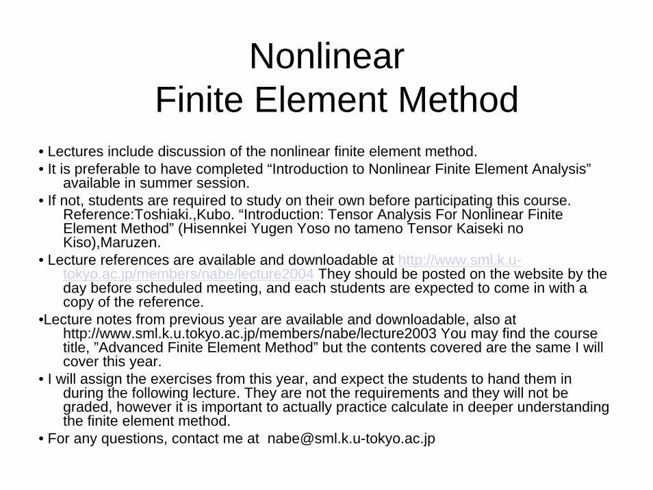
Nonlinear Finite Element Method

• Lectures include discussion of the nonlinear finite element method.• It is preferable to have completed “Introduction to Nonlinear Finite Element Analysis”

available in summer session.• If not, students are required to study on their own before participating this course.

Reference:Toshiaki.,Kubo. “Introduction: Tensor Analysis For Nonlinear Finite Element Method” (Hisennkei Yugen Yoso no tameno Tensor Kaiseki noKiso),Maruzen.

• Lecture references are available and downloadable at http://www.sml.k.u-tokyo.ac.jp/members/nabe/lecture2004 They should be posted on the website by the day before scheduled meeting, and each students are expected to come in with a copy of the reference.

•Lecture notes from previous year are available and downloadable, also at http://www.sml.k.u.tokyo.ac.jp/members/nabe/lecture2003 You may find the course title, ”Advanced Finite Element Method” but the contents covered are the same I will cover this year.

• I will assign the exercises from this year, and expect the students to hand them in during the following lecture. They are not the requirements and they will not be graded, however it is important to actually practice calculate in deeper understanding the finite element method.

• For any questions, contact me at nabe@sml.k.u-tokyo.ac.jp

Nonlinear Finite Element Method Lecture Schedule

1. 10/ 4 Finite element analysis in boundary value problems and the differential equations2. 10/18 Finite element analysis in linear elastic body3. 10/25 Isoparametric solid element (program)4. 11/ 1 Numerical solution and boundary condition processing for system of linear

equations （with exercises）5. 11/ 8 Basic program structure of the linear finite element method(program)6. 11/15 Finite element formulation in geometric nonlinear problems(program)7. 11/22 Static analysis technique、hyperelastic body and elastic-plastic material for

nonlinear equations (program)8. 11/29 Exercises for Lecture79. 12/ 6 Dynamic analysis technique and eigenvalue analysis in the nonlinear equations10. 12/13 Structural element11. 12/20 Numerical solution— skyline method、iterative method for the system of linear

equations12. 1/17 ALE finite element fluid analysis13. 1/24 ALE finite element fluid analysis

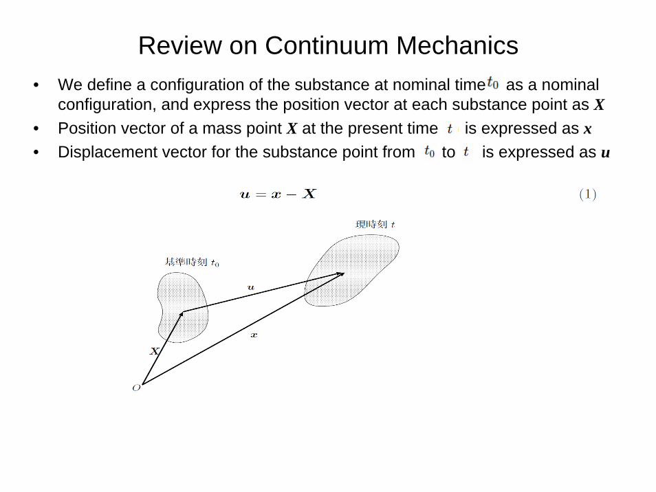
Review on Continuum Mechanics• We define a configuration of the substance at nominal time as a nominal

configuration, and express the position vector at each substance point as X• Position vector of a mass point X at the present time is expressed as x• Displacement vector for the substance point from to is expressed as u

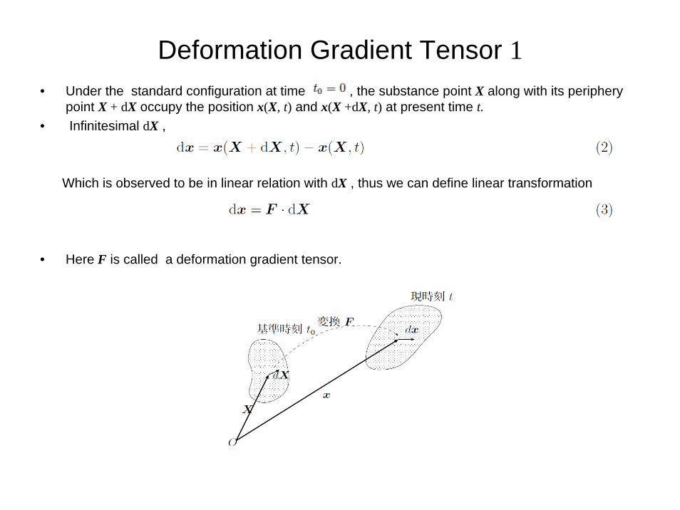
Deformation Gradient Tensor 1• Under the standard configuration at time , the substance point X along with its periphery

point X + dX occupy the position x(X, t) and x(X +dX, t) at present time t.• Infinitesimal dX ,

Which is observed to be in linear relation with dX , thus we can define linear transformation

• Here F is called a deformation gradient tensor.

Deformation Gradient Tensor 2• Generally, the deformation gradient tensor F is not in symmetry.• detF = 0 must not be established but, when the inverse relationship:

If the relation above exist in transformation, then the tensor is considered to be in symmetry.• Which refers that the substance points before the transformation dx and dX, correspond to the

points after the deformation respectively.• Generally, when we have an orthogonal tensor R and a positive symmetrical tensor U , the

deformation gradient F can be decomposed in the following,

• U is called a right stretch tensor, and this is called the right polar decomposition of the deformation gradient tensor.

• Likewise, having R as the same orthogonal tensor as seen in the right polar decomposition, and V as a positive symmetrical tensor,

The above is called the left polar decomposition of the deformation gradient tensor. V is called the left stretch tensor.

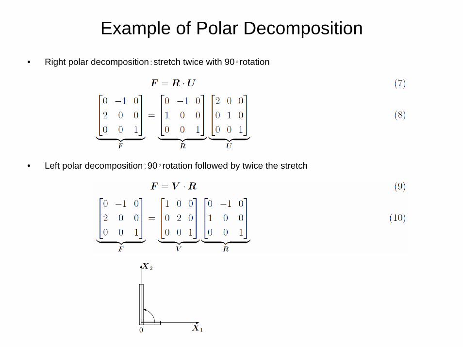
Example of Polar Decomposition

• Right polar decomposition：stretch twice with 90◦ rotation

• Left polar decomposition：90◦ rotation followed by twice the stretch

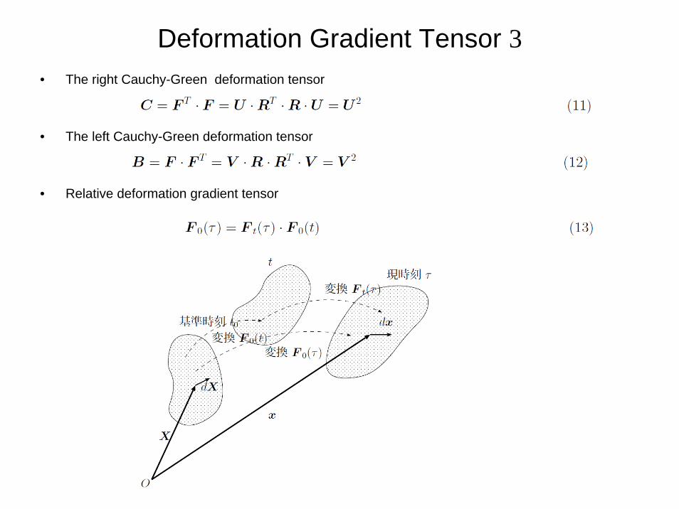
Deformation Gradient Tensor 3• The right Cauchy-Green deformation tensor

• The left Cauchy-Green deformation tensor

• Relative deformation gradient tensor

Strain 1

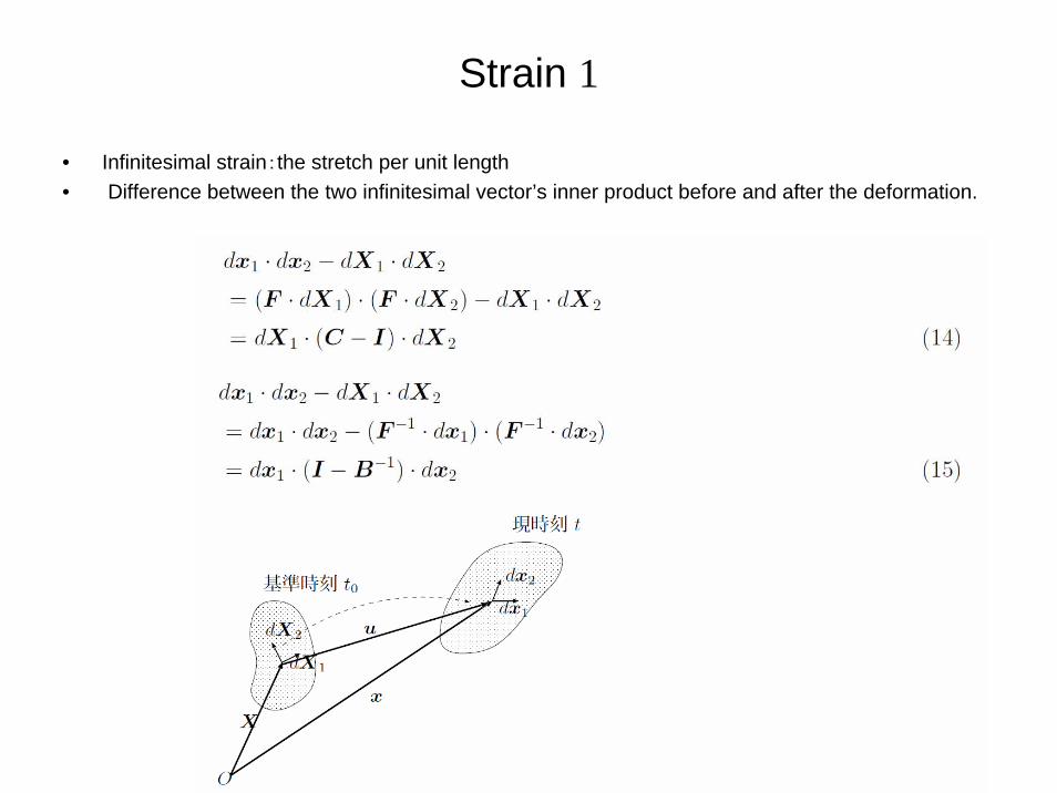
• Infinitesimal strain：the stretch per unit length• Difference between the two infinitesimal vector’s inner product before and after the deformation.

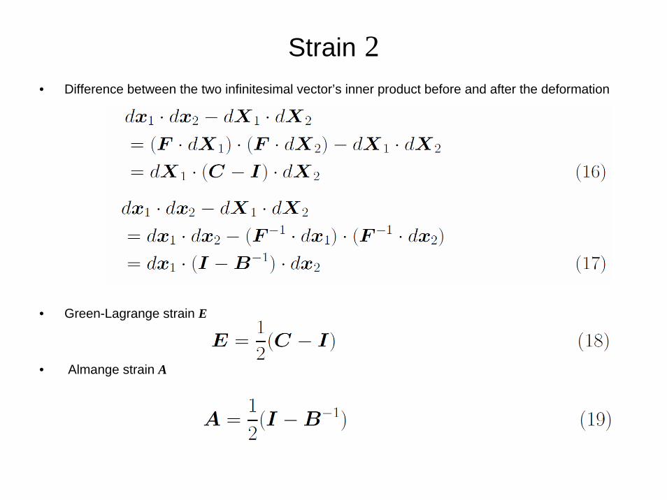
Strain 2• Difference between the two infinitesimal vector’s inner product before and after the deformation

• Green-Lagrange strain E

• Almange strain A

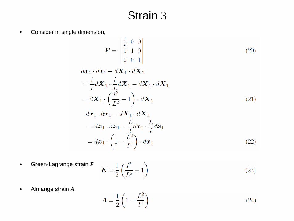
Strain 3• Consider in single dimension，

• Green-Lagrange strain E

• Almange strain A

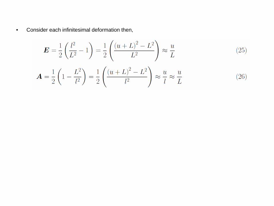
• Consider each infinitesimal deformation then,

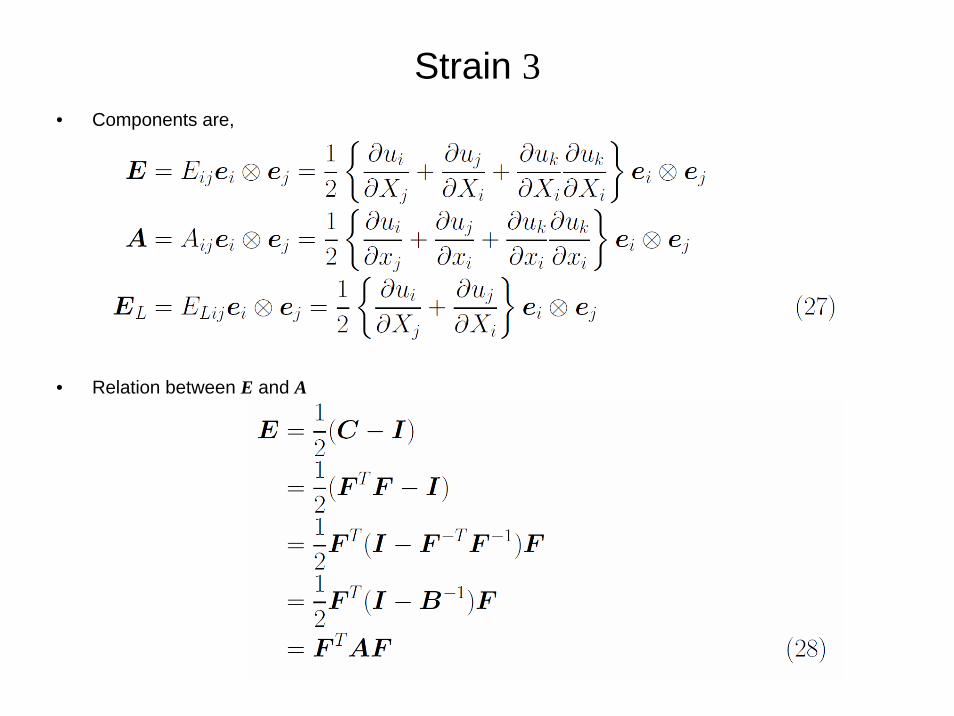
Strain 3• Components are,

• Relation between E and A

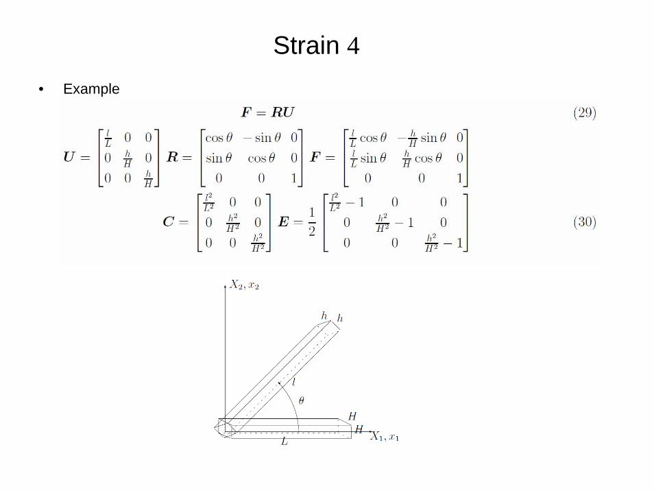
Strain 4• Example

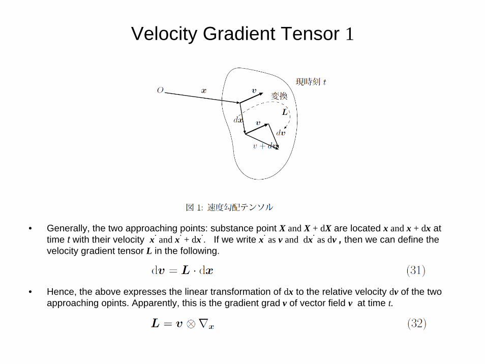
Velocity Gradient Tensor 1

• Generally, the two approaching points: substance point X and X + dX are located x and x + dx at time t with their velocity x˙ and x˙ + dx˙. If we write x˙ as v and dx˙ as dv , then we can define the velocity gradient tensor L in the following.

• Hence, the above expresses the linear transformation of dx to the relative velocity dv of the two approaching opints. Apparently, this is the gradient grad v of vector field v at time t.

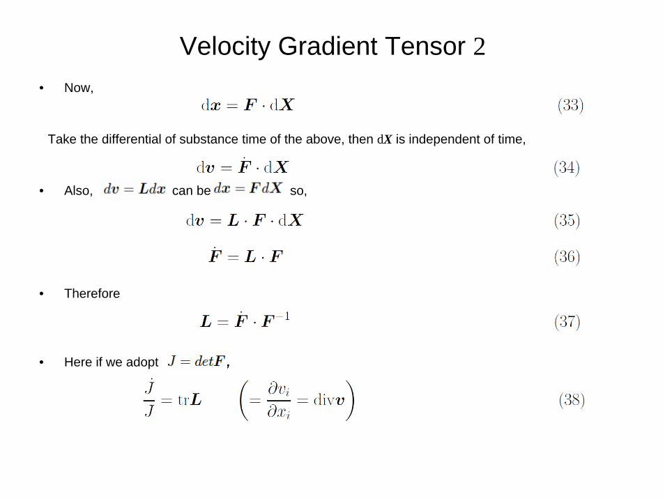
Velocity Gradient Tensor 2• Now,

Take the differential of substance time of the above, then dX is independent of time,

• Also, can be so,

• Therefore

• Here if we adopt ,

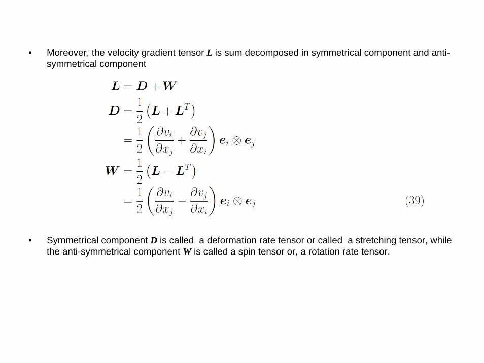
• Moreover, the velocity gradient tensor L is sum decomposed in symmetrical component and anti-symmetrical component

• Symmetrical component D is called a deformation rate tensor or called a stretching tensor, while the anti-symmetrical component W is called a spin tensor or, a rotation rate tensor.

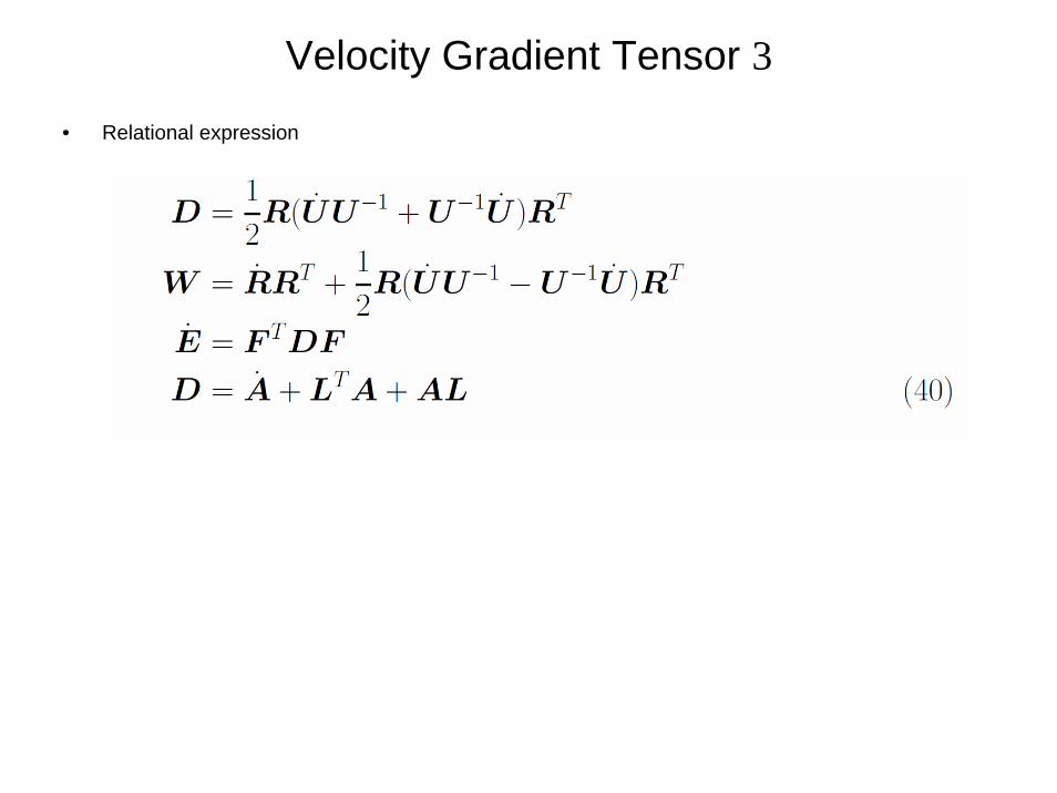
Velocity Gradient Tensor 3

• Relational expression

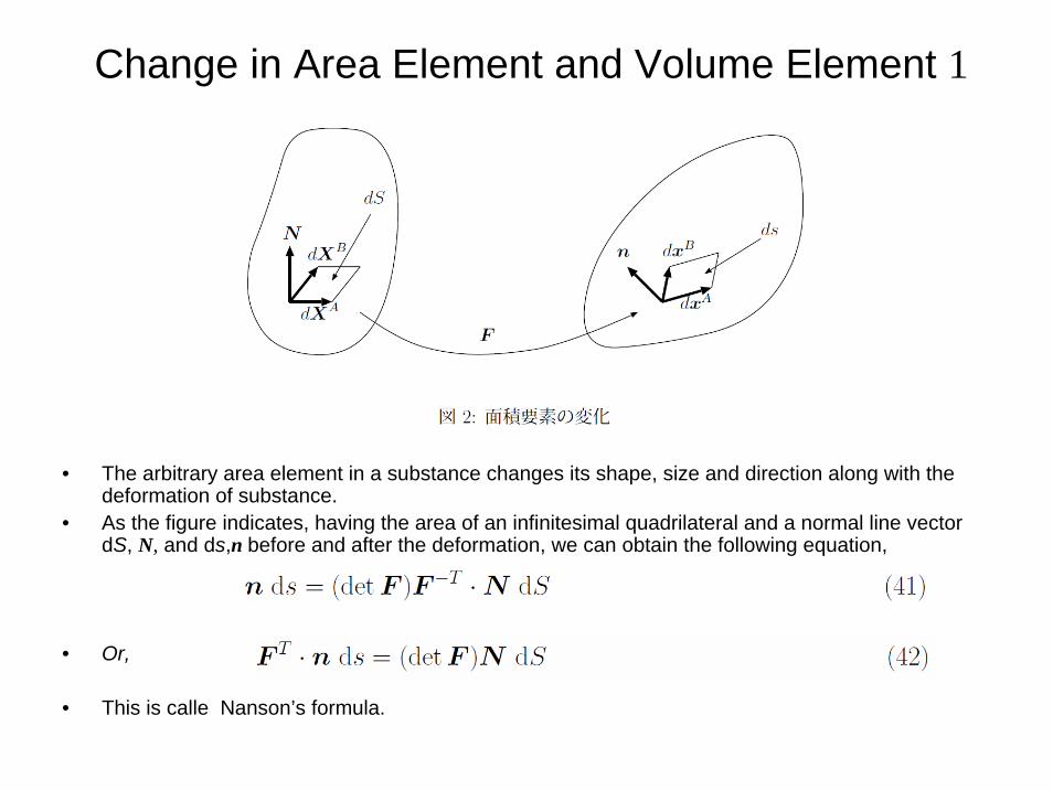
Change in Area Element and Volume Element 1

• The arbitrary area element in a substance changes its shape, size and direction along with the deformation of substance.

• As the figure indicates, having the area of an infinitesimal quadrilateral and a normal line vector dS, N, and ds,n before and after the deformation, we can obtain the following equation,

• Or,

• This is calle Nanson’s formula.

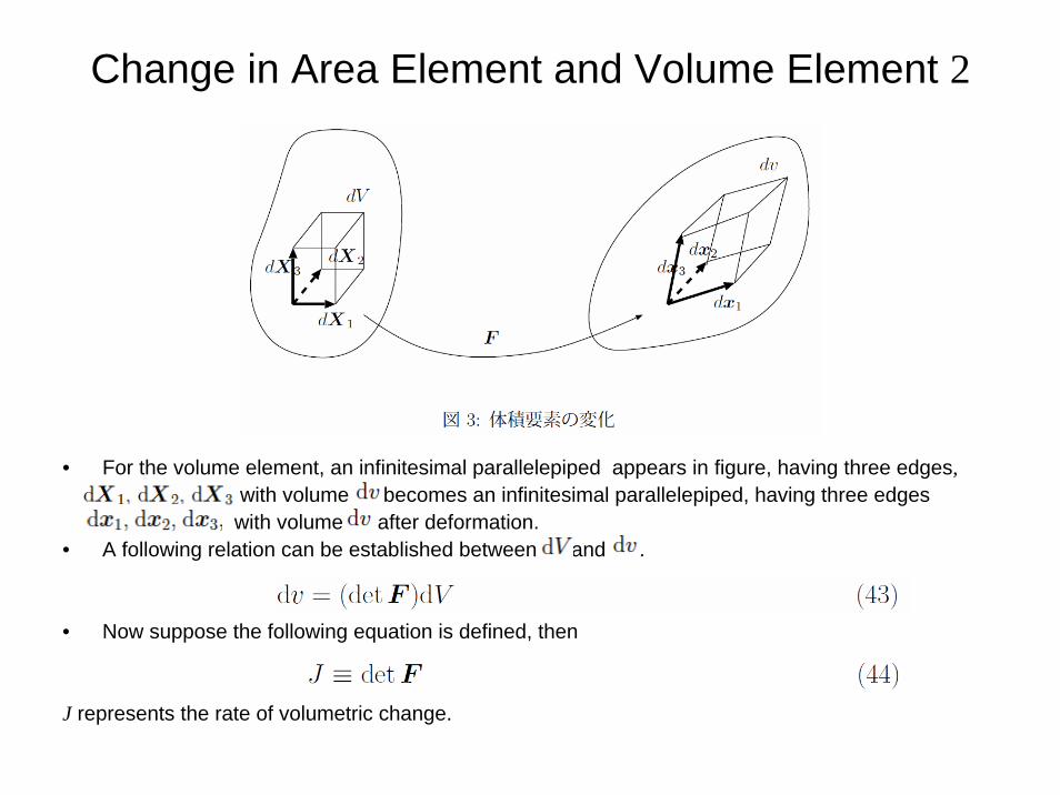
Change in Area Element and Volume Element 2

• For the volume element, an infinitesimal parallelepiped appears in figure, having three edges,with volume becomes an infinitesimal parallelepiped, having three edges

with volume after deformation.• A following relation can be established between and .

• Now suppose the following equation is defined, then

J represents the rate of volumetric change.

Principle of Conservation of Mass• The mass of substance m with mass density ρ, and a region occupied by substance v ,we can write as,

• Principle of conservation of mass stands for m to stay constant, and being independent of time, thus

• Here, ˙ represents a substance time derivative, and with ,

• If we take the time derivatives in above equation,

The above transformation can be established to the arbitrary part of the substance, also.

Principle of Conservation of Momentum 1• Force that acts on the substance includes a body force vector ρg and a surface force vector t. grepresents the body force per unit mass, while ρg represents the force acting on the unit volume. and, t represents the force acting on the unit area.

• The sum of these forces in total substance equals to the velocity of momentum , hence

• This is called Euler’s first law of motion.• Here ,we define v˙ ≡ a, so we use to express the following.

Principle of Conservation of Momentum 2• We obtain the following equation for the angular momentum.

• Therefore, the substance force, the surface force moment and the moment of momentum share the same velocity about the origin of the coordinates.

• This is called Euler’s second law of motion. In the left hand side, we have

thus

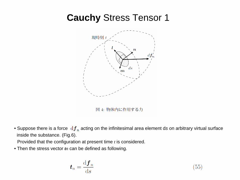
Cauchy Stress Tensor 1

• Suppose there is a force acting on the infinitesimal area element ds on arbitrary virtual surface inside the substance. (Fig.6).Provided that the configuration at present time t is considered.

• Then the stress vector tn can be defined as following.

Cauchy Stress Tensor 2

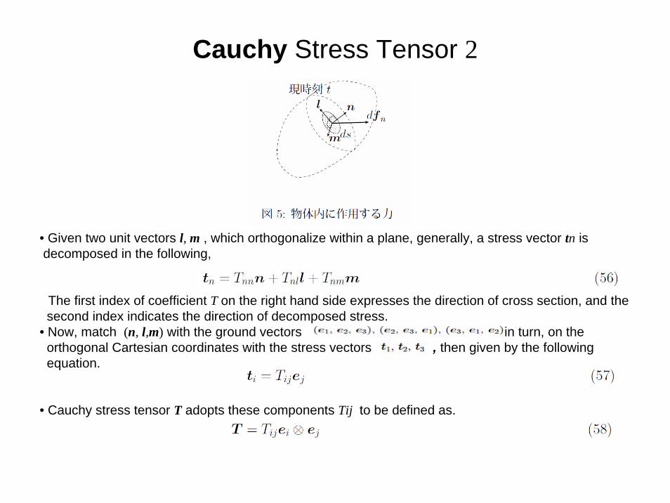
• Given two unit vectors l, m , which orthogonalize within a plane, generally, a stress vector tn is decomposed in the following,

The first index of coefficient T on the right hand side expresses the direction of cross section, and the second index indicates the direction of decomposed stress.

• Now, match (n, l,m) with the ground vectors in turn, on the orthogonal Cartesian coordinates with the stress vectors , then given by the following equation.

• Cauchy stress tensor T adopts these components Tij to be defined as.

Cauchy Stress Tensor 3

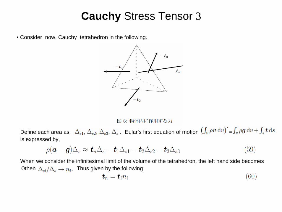
• Consider now, Cauchy tetrahedron in the following.

Define each area as ． Eular’s first equation of motion = is expressed by,

When we consider the infinitesimal limit of the volume of the tetrahedron, the left hand side becomes ０then Thus given by the following．

Cauchy Stress Tensor 4• When we substitute into , we obtain the following Cauchy’s formula :

• Cauchy’s formula can be formed on the surface of substance, also. By substituting into t in derived from Eular’s first law of motion, and by adopting the divergence theorem, we can obtain the following.

• Since this equation can be established for an arbitrary part of the substance,

or,

• This is called Cauchy’s first law of motion or an equilibriumequation.

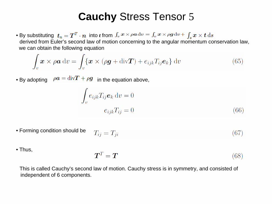
Cauchy Stress Tensor 5• By substituting into t from

derived from Euler’s second law of motion concerning to the angular momentum conservation law, we can obtain the following equation

• By adopting in the equation above,

• Forming condition should be

• Thus,

This is called Cauchy’s second law of motion. Cauchy stress is in symmetry, and consisted of independent of 6 components.

Various Stress Tensor

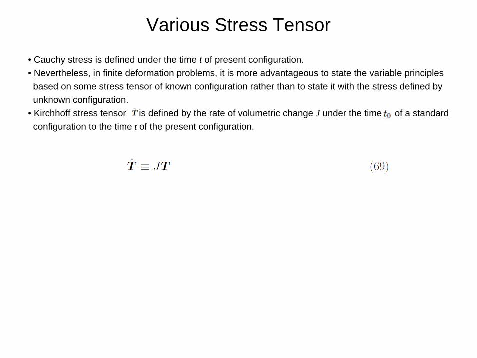
• Cauchy stress is defined under the time t of present configuration.• Nevertheless, in finite deformation problems, it is more advantageous to state the variable principles based on some stress tensor of known configuration rather than to state it with the stress defined by unknown configuration.

• Kirchhoff stress tensor is defined by the rate of volumetric change J under the time of a standard configuration to the time t of the present configuration.