Nuclear Engineering and Design 51 (1979) 389-401 389 © North-Holland Publishing Company

FINITE ELEMENT FORMULATION AND SOLUTION OF NONLINEAR HEAT TRANSFER

Klaus-Jfirgen BATHE and Mohammad R. KHOSHGOFTAAR Department of Mechanical Engineering, Massachusetts Institute of Technology, Cambridge, MA 02139, USA

Received 31 July 1978

A general and effective finite element formulation for analysis of nonlinear steady-state and transient heat transfer is presented. Heat conduction conditions, and convection and radiation boundary conditions are considered. The solutions of the incremental heat transfer equations is achieved using Newton-Raphson iteration, and in transient analysis using a one- step s-family time integration scheme. The stability and accuracy of the time integration is discussed. The solution tech- niques have been implemented, and the results of various sample solutions are discussed and evaluated.

1. Introduction

Since the advent of the electronic digital computer, the associated development of effective finite element procedures for stress analysis of structures and con- tinua [1,2], and the application of finite element techniques to the solution of heat transfer problems [3-5] , the predominant numerical method for anal- ysis of heat transfer problems remained the finite difference method. It is only during the very recent years that the advantages of a finite element analysis have become more clear. Apart from the benefits that can be obtained from the generality of the finite ele- ment method, e.g. to approximate geometries and material properties, emphasis on the development of effective finite element procedures for field prob- lems is also important, because the application of finite element methods shows much promise for the solu- tion of coupled stress and field problems [6].

The objective in this paper is to present a general and effective incremental finite element formulation for analysis of nonlinear steady-state and transient heat transfer, the numerical algorithms employed for solution and various experiences that have been gained in the evaluation of the solution procedures. The analysis techniques have been implemented in the computer program ADINAT and are employed for the solution of heat transfer problems with conduc- tion, convection and radiation conditions [7]. In this

work decoupled stress and temperature conditions are assumed, but the ultimate objective is also the develop- ment of effective solution techniques for analysis of coupled stress and field problems.

2. Finite element solution of nonlinear heat transfer

The governing equations for heat transfer analysis of a body idealized by a system of finite elements can be derived by invoking the stationarity of a func- tional or using the Galerkin method [2]. However, the realization that, physically, heat flow equilibrium is to be satisfied at the finite element nodes (and in an integrated sense throughout the finite element idealization) yields additional insight into the solu- tion process, and provides an effective basis for the development of the incremental heat flow equilibrium equations for linear and nonlinear steady.state and transient analysis.

2.1. Incremental fleM equations

As in incremental finite element stress analysis [2], assume that the conditions of the body at time t have been calculated, and that the temperatures are to be determined for time t + At, where At is the time increment. To evaluate the temperatures at time t + At the heat flow equilibrium of the body is considered

390 K.-J. Bathe, M.R. Khoshgoftaar / Nonlinear heat transfer

at time t + na t , where 0 < a < 1 and a is chosen to obtain opttmmn stability and accuracy in the solution. (In steady-state a n a l y ~ e = I and At is used to deter- mine the heat flow increment, but is otherwise a dummy variable.) Considezing heat flow equilibrium at time t + n a t the basic equation to be satisfied for a three-dimentional body is

f 6 0 ' r t+~at k t+aat o, t+aAt 0 d V

v

+ f 6os t + ~ t h ~ + a l t O e - t+aAtoS) dS

8c

+ . f ~ O S t+aAtg(t+o~AtOr -- t+aAtoS) d~ (1)

sr

where 0 is the temperature of the body, 0 s is the sur- face temperature, 0e is the environmental temperature, 0r is the temperature of a radiating source and the superscript t + ~ t denotes "at time t + nat". Also,

denotes "variation in", h is the surface convection coefficient, r is a radiation coefficient and

ay

° il k = ky ,

0

where kx, ky and kj are the thermal conductivities corresponding to the principal directions of conduc- tivity x, y and z.

In eq. (1)So andSr are the surface areas with con- vection and radiation boundary conditions respec- tively, and t+aatO is the virtual work of the external heat flow input to the system at time t + r, At. The quantity t+az~t0 includes the effects of surface heat flow inputs, qS, (that are not included in the convec- tion and radiation boundary conditions), internal heat generation, ~ B, and temperature-dependent heat capa- city, c. Hence

t+~AtQ = fsos t+~Atq S dS

s

+ f~o( t+~r4a- t+oLAtct+aAto)dV (2)

V

It should be noted that in linear analysis t+~Atk, t+~AtC and t+~ath are comtaat and radiation bound- ary conditiom are not included. Hence eq. ( l ) can be solved directly for the temperature t+~Ato, see eq. (9). However, in nonlinear analysis eq. (1) is a non- linear equation for the temperature at time t + r"xt. Using eq. (2) for steady-state analysis or transient analysis with implicit time integration { explicit time integration (case a = 0) is performed as in linear anal- ysis [2] } the solution is obtained effectively by lin- earizing eq. (1) as shown in table 1 and then using the modified Newton-Raphson iteration method. In this

Table 1 Linearization of nonlinear heat flow equilibrium equations

1. Equilibrium equations at time t + ~At

J 6 0 ' T t+~At k t+~At O, t+~At(~ dV

V

/ 60 S t+~Ath(t+~Ato e -- t+~AtoS) dS +

$c

f 60 S t+~Atr(t+UAtor -- t+c~AtoS)dS +

Sr

2. Linearization of equations We use:

t+~Ato = to +0 ; t+~At~ = t o , +O o ; t+~At k= t k + k ;

t+~Ath = th + h ; t+~At~ = t~ + r

and assume:

t+aAtk t+aAt0' = tk(t0' +0') ;

t+aAth(t+~Ato e _ t+~AtoS ) = th(t+~A to e _ toS _ 0 s)

t+~Atg(t+~AtOr _ t+~AtoS ) = tg(t+~AtOr _ toS _ 0 s)

Substituting into the equations of heat flow equilibrium we obtain

f 6o'T tkO' dV + f 6oS th oS ds + f ~oS t~ oS dS

V S c Sr

t+~AtQ+ f 60 S th(t+'~Atoe _ toS ) dS

8e

+ [ ~ 0 s t,,(t~Ato r - tO s) dS - f i e ' r t k t o , dV

sr v

K.-Z Bathe, M.R. Khoshgoftaar / Nonlinear heat transfer 391

iteration we solve, for i = 1,2, ...,

f ~ o ' T t k A0 '(/) dV+ fsoS th A0S(i) dS

V Sc

+ / ~0 S tg A0s(i) dS = t+~AtQ

sr

+ / ~0 S t+etath(i-l)(t+otAtOe -- t+¢XAtoS(i-1)) dS

Sc

+ f 808 t+~Atg(i--1)(t+¢XAto r -- t+¢XAto$(i--l)) (iS

Sr

- f so 'T t+aAtk(i-1) t+aato'(i-1) dV, v

where

t+~Ato(i) = t+aAto(i--1) + A0(i) ,

(3)

(4) and t+aZ~th(i-O, t cea t l¢ ( i - l ) , and t+aAtk( i -1) are the

convection and radiation coefficients and the con- ductivity matrix that correspond to the temperature t+~Ato(t-1)"

In transient analysis t+aatQ is a function of t+aAto, which is approximated using a time integration scheme as discussed in section 2.4.

2.2. Finite element discretization

It is effective to employ isoparametric finite ele- ment discretization, in which we use for an element [2]:

N N N

x = ~ hix i; y = ~ hiYi; z= ~ hizi, (5) i= 1 i = 1 i= 1

and

N N

t4ctAt 0 = ~ h i t4ctAtot; t o = ~ h i t o i , i = 1 i = 1

N

AO = ~ hi AOi, (6) i= I

where the hi are the element interpolation functions; N is the number of nodal points; xi, Yi, zi are the coordinates of nodal point i, and t+aZ~tot, tot, A0i are the temperatures at times t + czAt, t and temperature

increment at nodal point i. Eq. (5) has been written for a three-dimensional element; for a one- or two- dimensional element only the appropriate coordinate interpolations would be employed.

The finite element incremental heat flow equili- brium equations are derived by substituting the inter- polations of eqs. (5) and (6) into eqs. (2) and (3). As usual, only a single finite element is considered, because the equilibrium equations of the complete system of finite elements are obtained by assemblage of the individual finite element matrices [2]. Table 2 summarizes the finite element matrices that are obtained from eqs, (2) and (3), when the interpola- tions in eqs. (5) and (6) are substituted. Using the results of table 2, eqs. (2) and (3) are thus for a single finite element:

( tKk + tKC + tKr ) A0(i) = t+~AtQ

+ t+~AtQC(i-1) + t+~AtQr( i - l ) _ t+~AtQk( i - l ) ,(7)

where

t+~Ato(i) = t+~Ato(i-1) + A0 (i) • (8)

Considering table 2 it should be noted that the tem- perature interpolation matrices, H and H s, are directly constructed from the element interpolation functions, and the temperature gradient interpolation matrices, B, are obtained from the derivatives of the interpola- tion functions as described in [2,p. 187].

Eq. (7) is the general incremental heat flow equi- librium equation, that is valid for linear and nonlinear analysis. However, in linear analysis, the equation can be used in a more effective form. Namely, if the con- ductivity, specific heat and convection coefficients are constant, i.e. tKk and tKC are constant matrices, and radiation boundary conditions are not included, eq. (7) becomes:

(K k + K c) t+~At 0 = t+~AtQ + t+~AtQe (9)

where K ¢ and t+¢XAtQe are defined in table 2.

2. 3. Incorporation of boundary conditions

Convection and radiation boundary conditions are taken into account by including the matrices tK¢ and tKr and the vectors t-mAtQ e and t+aat{~ in the heat flow equilibrium equations, eq. (7). Additional exter- nal heat flow input on the boundary is specified in t4~AtQ as surface heat flow input (see table 2).

392

Table 2 Finite element matrices

Integral

f s 0 ' T t k A0,(i) d V

K.-J. Bathe, M.R. Khoshgoftaar / Nonlinear heat transfer

Finite element evaluation

tKk A0 (i) = ( ;B T tk B dIO A0 (i)

V

f so s th ~oS(i) dS Se

f SO S t K AoS(i) dS

Sr t+~AtQ [in eq. (2)]

f 60 s - dS t+aAth(i-- l )(t+aA to e t+~AtoS(i-1) )

Sc

f SO S - dS t+aAtK(i- l )(t+aAtor t+aAtoS(i-1) )

Sr

f so T t+a~tk(i-1) t+aAto'(i-1) dV

V

f h 80 S t+c~AtoS dS

Se

f h 80 S t+ahto e dS

Sc

v

tKC A0 (i) = ( ; th H ST H S dS) A0 (i)

Sc

tKr A0(i) = ( ; t~ HSTH S dS) A0 (i)

Sr t+aAtQ(i- 1) = t+aAt~ _ t+aA Pc(i- 1 ) t+aA tO(i- 1 )

t+aAt~= / H T t+aAt~B dV +fH sT t+aAtqS dS

V S

t+~A tc(i- 1) = f t+~te(i- ~ ) H T H dV V

t+cgAtQe(i--l ) = f t+~Ath(i-1 ) H ST[HS(t+aAt Oe

Sc --t+aAto(i- 1))1 dS

t+aAtQr(i-1) = f t+aAtK(i--1 ) HST [HS(t+~At0r

Sr

- t+c~At0(i-1))] dS

t+aAtQk(i-l) = f BT[t+aAtk(i-1)B t+c~Ato(i-1) ] dV

V

K c t+~At0 = ( ; h H ST H S dS) t+aAt0

Sc

t+aAtQe : f h HST[H S t+~At0e] dS

Sc

The only boundary conditions that have not yet been taken into account in eq. (7) are temperature boundary conditions. Zero temperature conditions at a nodal point are simply imposed by not including the heat flow equilibrium equation corresponding to that nodal point. In order to specify a nonzero tem- perature condition, it is effective to employ the pro- cedure that is used to impose convection boundary conditions. Namely, by specifying a large value of h the surface temperature will be equal to the applied temperature.

2.4. Step-by-step time integration

Considering the finite element heat transfer equi- librium equations, we recognize that for any time t these equations can be written in the form,

CO + KO-- O, (10)

where C is the heat capacity matrix, Q is a vector of thermal nodal loads and

K = K k + K c + K r . (11)

K.-J. Bathe, M.R. Khoshgoftaar / Nonlinear heat transfer 393

In eq. (10) the matrices C and K and the vector Q are in general temperature dependent.

2.4.1. Time integration schemes For transient analysis it is effective to employ

numerical time integration [2]. In this study we con- sider a family of one-step methods with the following assumptions [8-10] :

t+aAto = (t+£xt 0 _ t O ) / A t , (12)

and

t+aato = (1 - a) tO + olt+Ato . (13)

Using eq. (10) at time t + aAt [as was done in the formulation, eq. (7)], and the assumptions in eq. (12) and (13)we obtain for an effective incremental solu- tion the equations corresponding to an Euler for- mula with time step aAt,

ao t+aAtc t+At/alO + t4~AtK t+aAto

= t+~AtO + ao t+aAtc t o , (14)

and also

t+Ato = a l t+At/alO + (1 -- a l ) to , (15)

where

ao =(At) - t , a l = l f o r a = 0 ,

ao = (aAt) -1 , al = a -1 for a 4: 0 .

In the above scheme we have the Euler forward method when a = 0 and the Euler backward method when a = 1 [2].

Since, in nonlinear analysis, t+~a~{} must be cal- culated by an iterative technique, we employ for the assemblage of elements:

t+aato(i) = (t+aAto(i--1) + A0( i ) _ to ) / (aAt )" (16)

This relation is obtained from eqs. (12) and (13) by e l i m i n a t i n g t+Ato and then using eq. (8).

2.4.2. Stability and accuracy The stability of the time integration scheme is

analyzed as usual by considering the single degree-of- freedom nonlinear heat transfer equation

b +X(0, t)O = 0 , (17)

where it is assumed that the effect of temperature dependent loads is negligible. Using the integration

scheme we obtain:

[I - (1 - a) At t+aAt~ 7 t+At 0

1 + aAtt T(62XT~ d to (18)

where for stability:

1 -- (1 -- a) At t+aAtx T + a A t ~ - ~ / ~ ~ 1. (19)

Here, it should be noted that k contains the effects of conduction, convection and radiation, because the convection and radiation matrices are in eq. (10) simply added to the conduction matrix. From eq. (19) we obtain the following results:

(i) for a/> ~ the scheme is unconditionally stable; (ii) for a < ~ the scheme is stable provided At <~

2/[(1 - 2a) t+~Atx].

The solution accuracy of the scheme is also anal- yzed considering eq. (17). Of particular interest are the Euler forward method (a = 0), the trapezoidal rule (a = 1) and the Euler backward method (a = 1). 2 To identify the accuracy of the Euler forward method we employ the Taylor series expansion

At 2 tb. + At3 t. 0. .... t+ato = to + At t~ + ~ . ~f. + (20)

and obtain by rearranging:

At t~ At2c'" tO = (t+ato -- to) /At - ~ - -f(f. 0 - .... (21)

Similarly, to identify the accuracy of the Euler back- ward method, we can obtain

= (t+z~t 0 _ t o ) / A t +~t.t+At" O" _ At2 t+At. ~. + - ... . t+AtO 2v • 3 !

(22)

Eqs. (21) and (22) show that both Euler methods are first-order accurate. However, in the Euler back- ward method the terms that are truncated to repre- sent the time derivative approximately [compare eqs. (12) and (22)] alternate in sign, which can result in significantly better solution accuracy using this method•

To identify the accuracy of the trapezoidal rule we recognize that the total solution for t+ato involves a backward Euler step and then a forward Euler step each with time step At~2. Thus, using backward and forward Taylor series expansions about t + At~2 for to and t+ato, respectively, we obtain using eq. (17)

394 K.-J. Bathe, M.R. Khoshgoftaar / Nonlinear heat transfer

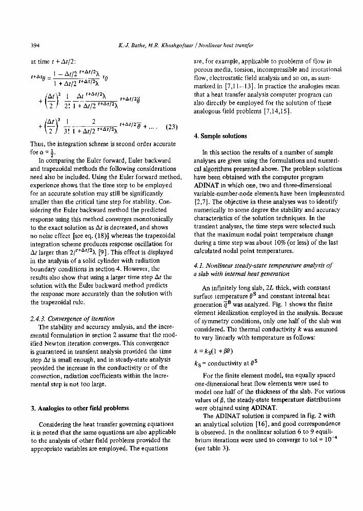
at time t + At/2:

t+At 0 = 1 - At~2 t+At/2~k to 1 + At~2 t+At/2~k

( A t f 1 At t+At/2x t+At/2~ + - - 2~ 1 +At~2 t+at/2X

(~t)3 1 2 t+At/2ff + ~ 3T. 1 +At~2 t+Atl2~ + .... (23)

Thus, the integration scheme is second order accurate for a = ½.

In comparing the Euler forward, Euler backward and trapezoidal methods the following considerations need also be included. Using the Euler forward method, experience shows that the time step to be employed for an accurate solution may still be significantly smaller than the critical time step for stability. Con- sidering the Euler backward method the predicted

response using this method converges monotonically to the exact solution as At is decreased, and shows no noise effect [see eq. (18)] whereas the trapezoidal integration scheme produces response osciUation for At larger than 2/t+At/g~k [9]. This effect is displayed in the analysis of a solid cylinder with radiation boundary conditions in section 4. However, the results also show that using a larger time step At the solution with the Euler backward method predicts the response more accurately than the solution with the trapezoidal rule.

2. 4. 3. Convergence o f iteration The stability and accuracy analysis, and the incre-

mental formulation in section 2 assume that the mod- ified Newton iteration converges. This convergence is guaranteed in transient analysis provided the time step At is small enough, and in steady-state analysis provided the increase in the conductivity 9r of the convection, radiation coefficients within the incre- mental step is not too large.

3. Analogies to other field problems

Considering the heat transfer governing equations it is noted that the same equations are also applicable to the analysis of other field problems provided the appropriate variables are employed. The equations

are, for example, applicable to problems of flow in porous media, torsion, incompressible and irrotational flow, electrostatic field analysis and so on, as sum- marized in [7,11-13]. In practice the analogies mean that a heat transfer analysis computer program can also directly be employed for the solution of these analogous field problems [7,14,15 ].

4. Sample solutions

In this section the results of a number of sample analyses are given using the formulations and numeri- cal algorithms presented above. The problem solutions have been obtained with the computer program ADINAT in which one, two and three-dimensional variable-number-node elements have been implemented [2,7]. The objective in these analyses was to identify numerically to some degree the stability and accuracy characteristics of the solution techniques. In the transient analyses, the time steps were selected such that the maximum nodal point temperature change during a time step was about 10% (or less) of the last calculated nodal point temperatures.

4.1. Nonlinear steady-state temperature analysis o f a slab with internal heatgeneration

An infinitely long slab, 2L thick, with constant surface temperature 0 s and constant internal heat generation ~B was analyzed. Fig. 1 shows the finite element idealization employed in the analysis. Because of symmetry conditions, only one half of the slab was considered. The thermal conductivity k was assumed to vary linearly with temperature as follows:

k = ks(1 +/30)

k s = conductivity at 0 s

For the finite element model, ten equally spaced one-dimensional heat flow elements were used to model one half of the thickness of the slab. For various values of/~, the steady-state temperature distributions were obtained using ADINAT.

The ADINAT solution is compared in fig. 2 with an analytical solution [16], and good correspondence is observed. In the nonlinear solution 6 to 9 equili- brium iterations were used to converge to tol = 10 -4 (see table 3).

K.-J. Bathe, M.R. Khoshgoflaar / Nonlinear heat transfer 395

ct)

O S . . - ~

MATERIAL MODEL:

k=ks(l+BO)

~x

oo

-,-----~_ oS

's• ~=tona k ks= conductivity of

material at 0 s " O

Are°=l FINITE ELEMENT MODEL /_

IO EQUALLY SPACED ONE-DIMENSIONAL ELEMENTS FOR HALF OF THE SLAB

Fig. 1. Nonlinear temperature analysis o f slab with internal heat generation.

4.2. Transient temperature analysis of a slab subjected to simultaneous boundary convection and radiation

The slab shown in fig. 3 is initially at a uniform t e m p e r a t u r e 0 i . At time t = 0 ÷ the slab surfaces are exposed to convection (temperature 0e = 0, heat transfer coefficient h) and radiation (temperature O r = 0, shape factor F, emissivity e). The thermal con- ductivity k and heat capacity c are assumed constant.

In the analysis using ADINAT the Euler backward method was employed. The solution for 0 s (surface temperature) and 0 c (temperature at the center of the slab) depends upon two parameters, Bi and r'. Figs. 4 and 5 show the temperature variations at the sur- face and at the center, respectively, for Bi = 0.2, 4, and for radiation parameters r of 0 and 4. The ADI- NAT solutions compare well with solutions obtained by Haji-Sheikh and Sparrow [17], who used a prob- ability method.

In order to obtain the required accuracy in the

LO'

Q:,OD IO"

0.9

0.8

0.7

0.6

0.5

Ok

0.5

0.2

0.1

/~aL2/Zk,:O0

~ 02

04

0.6

- - ANALYTICAL SOLUTION

ADINAT SOLUTION

0.0 I i I I 0.0 02 0.4 0.6 0.8 Lo

x /L

Fig. 2. Steady state temperatures of slab with internal heat generation and temperature dependent conductivity.

ADINAT analysis the time step was changed during the response predictions. Table 4 summarizes the time step selections and gives the number of iterations used.

4.3. Transient temperature analysis of a solid cylinder subjected to simultaneous boundary convection and radiation

The solid cylinder shown in fig. 6 initially at a uni- form high temperature Oi is allowed to cool in air. The cylinder surface exchanges energy with the air by convection and radiation. The thermal conductivity k and heat capacity c of the cylinder are assumed con- stant. Since the cylinder is infinitely long, heat trans- fer takes place in the radial direction only.

The solution for 0 s (surface temperature) and 0 ¢ (temperature at the center of the cylinder) depends upon three parameters, Bi, r ' and 0e/0 i. Figs. 7 and 8

396 K.-J. Bathe, M.R. Khoshgoftaar /Nonl inear heat transfer

Table 3 Summary o f step-by-step integration

INITIAL CALCULATIONS tI( = L D L T

1. Form linear conductivity matrix K, linear heat capacity matrix C,

2. Initialize the following constants: tol < 0.01 ; nitem t> 3; f o r a = 0 :a0 = l / A t , al =1 for a :~ 0: ao = 1/c~At, al = 1/c~

3. Calculate effective linear conductivity matrix: f o r ~ = 0: l( = aoC and go to A f o r c ~ : ~ 0 : I ( = K k + K c + a o C

4. In linear analysis, triangularize I(.

FOR EACH TIME STEP

A. In linear analysis, a ~ 0 (i) Compute effective heat flow vector:

t+~tAQ = t+aAt~ + t+aAtQe + aoC tO

(ii) Solve for nodal point temperatures at time t + At

I( t+eeAt 0 = t+eAt O

t+At0= al t+°eAt0 + (1 - a l ) tO

B. In linear and nonlinear analysis i f e = 0: (i) If a new heat capacity matrix ( tc) is to formed,

update l i to obtain tI(,

t~[ = a 0 t c

(ii) Compute effective heat flow vector: t 0 = t ~ + t Q C + t Q r _ t Q k + a 0 t C t 0

(iii) Solve for nodal point temperatures at time t + At:

tI( t+AtO= t o

C. In nonlinear analysis i f ,~ ~ 0: (i) If a new conductivity matrix (tKk), nonlinear heat

capacity matrix ( tc) , nonlinear convection matrix (tKC), or radiation matrix (tKr) is to be formed, up- date I( to obtain t l ( and factorize t~,

tl( = tKk + tKC + tKr + a0 t c

(ii) Compute effective heat flow vector: t+~At 0 = t+c~At~ + tQC + tQr _ tQk

(iii) Solve for increments in nodal point temperatures using latest D, L factors:

L D LTo = t+~At 0

(iv) If required iterate for heat flow equilibrium; then initialize

0 (0)= 0, i = 0

(a) i= i+ 1

(b) Calculate (i - 1)st approximation to nodal point temperatures and time derivatives of nodal point temperatures:

t + a A t o ( i - l ) = t0+0( i - -1 ) ;

t + a A t 6 ( i - l )= ao( t+aAto( i -1 ) _ tO)

(c) Calculate ith out-of-balance heat flow rates: t+c~AtO(i-I ) = t+c~AtQ(i-1) + t+aAtQc( i -1 )

+ t+c~AtQr(i-1) _ t+aAtQk(i--1)

(d) Solve for ith correction to temperature increments: L D L T A0 (i) = t+aAtO( i -1 )

(e) Calculate new temperature increments:

0(i) = 0 ( i -1 ) + A0(i)

(f) Iteration convergence if IIAO(i)ll2/f = At, .~.. , t + AtlJ0112 < to1

If convergence: 0 = 0 (i) and go to (v); If no con- vergence and i < nitem: go to (a); otherwise restart using a new matrix reformation interval and/or a small time step size.

(v) Calculate new nodal point temperatures

t+At 0= t 0 + a l 0

show the temperature variations at the surface and at the center of the cylinder, respectively, for 1.0 ~< Bi~< 10, F = 1, and 0 e / 0 i = 0.55.

In the figures the ADINAT solutions are compared with the finite difference solutions obtained by SUCEC and KUMAR [18] and good correspondence in the results is noted.

In this analysis the Euler backward method and

trapezoidal rule have been used with the time step sizes summarized in table 5.

Some characteristics of the time integrations in a typical analysis of the problem are shown in fig. 9. It is seen that, using the Euler backward method, as the time step is decreased the predicted response con- verges uniformly to the response calculated with a very small time step, whereas, using the trapezoidal

K.-J. Bathe, M.R. Khoshgoftaar /Nonlinear heat transfer 397

CO

SIMULTANEOUS BOUNDARY~~ -

t - i CONVECTION AND RADIATION

L 00

MATERIAL MODELS :

SIMULTANEOUS BOUNDARY CONVECTION AND RADIATION

ee=er=O.O

k = conductivity, constant

h= convection coefficient, constant

E = emissivity coefficient, constant

Area = I FINITE ELEMENT MODEL _ _;_ . . . . . . . . . . . ; : = ~..; ; _...~_convection and . . . . . . . . . . . . . . radiation

2_0 EQUALLY SPACED ONE-DIMENSIONAL ELEMENTS FOR HALF OF THE SLAB

Fig. 3. Nonlinear temperature analysis of slab with rad ia t ion- convection boundary conditions.

1.0 - - o . 0

z

. 6 . 4

8 i , 8 i HAJ'-SHE'KH AND ~ ~ / .4 SPARROW / ~ / "O.J .6

.2 , e, ~.x~ /. ~ .8

I J I I I i J 1 I I I I I 61.0 02 4 6 810 -2 2 4 6 810 -I 2 4 6 8100 2 4

(:[ t / L 2

~F~8~L r : k

Bi=-~-

~= k._.~_ pc

Fig. 4. Transient temperature results for a slab wi th rad ia t ion- convection boundary condit ions, Bi = 0.2.

398 K.-J. Bathe, M.R. Khoshgoftaar / Nonlinear heat transfer

I0 0

.6 r=o. ~ Bi=h L 4.0 e c

z : - ~ - i co= p_.~ - .4 4. ~- HAJI-SHEIKH AND~ 0 . ~ / .6

2 4 6 810 -2 2 4 6 810 -~ 2 4 6 810 ° 2 4 6 ~t/k. 2

Fig. 5. Transient temperature results for a slab with radiation- convection boundary conditions, Bi -- 4.0.

m e t h o d with a large t ime step, the calculated response

oscillates about the accurate solution.

4. 4. Linear transient heat transfer analysis o f a solid block subjected to convection cooling

The solid block in fig. 10 is init ially at a un i form

temperature 400°F . The block surfaces are suddenly

exposed to convect ion condi t ions wi th a cons tant

convect ion coeff icient .

For the finite e lement analysis, 45 three-dimen-

sional 8 node e lements were used to mode l one quar-

ter o f the solid block. Fig. 11 gives the tempera tures

at points A and B (see fig. 10), as calculated using

ADINAT and in an analytical solut ion [16]. Good

correspondence be tween the results is observed.

In this analysis the trapezoidal rule has been used

for the t ime integrat ion and to obtain good solut ion

accuracy, the t ime step was changed during the res-

ponse predictions. Table 6 summarizes the t ime step

selection and gives the solut ion accuracy (measured on the analytical solution).

Table 4 Transient analysis of a slab with radiation-convection boundary conditions

Shape factor F = 1 emissivity e = 1 (black body) thermal diffusivity a = 1 in2/h tol = 1 X 10 -4 Euler backward method used

L = l i n o = 0.118958 X 10 -1° Btu/in: • h • °R4 k = 0.01 Btu/in • h • °F

Biot number t* = ~t/L 2 &talL 2 Number of average number time steps of iterations

Bi = 0.2 0 < t* < 0.08 0.002 40 3 0 <~ r < 4 0.08 < t* ~ 0.88 0.02 40 2

0.88 < t* ~ 3.88 0.05 60 2

Bi = 4.0 0 < t* ~ 0.06 0.001 60 3 0 ~ F ~ 4 0.06 < t* ¢ 0.66 0.01 60 2

0.66 < t* ~ 3.66 0.05 60 2

K.J. Bathe, M.R. Khoshgoflaar /Nonlinear heat transfer 399

Table 5 Transient analysis of a solid cylinder with radiation-convection boundary conditions

Shape factor F = 1 emissivity e = 1 (black body) thermal diffusivity ~ = 1 in2/h Euler backward method (E.B.)

o = 0.118958 × 10 -1° Btu/in 2 • h. °R4 k = 0.5238 Btu/in • h. °F Trapezoidal integration rule (T.R.) tol = 1 X 10 -3

t * Biot = ~t/r~ number

A t air 2 Number of time Average number of steps iterations

E.B. T.R. E.B. T.R. E.B. T.R.

Bi = 10 0 < t* < 0.01 0.0005 I ~ = 1 0.01 < t* < 0.21 0.005 0e/0 i = 0.55 0.21 < t* < 1.21 0.05

Bi = 2 0 < t* < 0.04 0.002 r = 1 0.04 < t* < 0.44 0.02 0e/0 i = 0.55 0.44 < t* < 1.44 0.1

0.001 20 10 2 2 0.01 40 20 2 2 0.05 20 20 1 1

0.004 20 I0 2 2 0.02 20 20 1 1 0.1 I0 10 I 1

5. Conclusions

A general and effective finite element solution scheme for the analysis of linear and nonlinear steady-

I i

simultaneous boundary _ _ . ~__ ._ ~ c o n v e c t i o n and radiation

0° .o ,

i MATERIAL MODELS:

c = heat capacity, constant k = conduct iv i ty , constant h = convection coeff icient, constant c = emissivity coefficient, constant

, ir o .075ro 1 .0Sro .O25ro

~J~ _ _ _ ~ convection and

AXISYMMETRIC FINITE E L E M E N T MODEL

Fig. 6. Nonlinear temperature analysis of an inf'mite solid cylinder with radiation-convection boundary conditions.

state and transient heat transfer problems has been presented. Conduction, convection and radiation

conditions are considered. The solution is achieved using isoparametric finite element discretization and direct time integration with a one step a-family inte- gration scheme. This family includes the conditionally

stable Euler forward method and the unconditionally stable Euler backward and trapezoidal methods. The

solution procedures have been implemented and in the paper the results of various sample analyses are given. Based on the experience gained in the use of the solution techniques, it is concluded that the meth-

ods can be employed effectively to obtain accurate

response predictions, but the nature of the transient

heat transfer response may require a varying time step At in the analysis.

Table 6 Transient analysis of a solid block with convection cooling (Using trapezoidal rule)

t At Number Max. error (h) (h) of time measured on

steps analytical solution (%)

0 < t < 1 0.1 10 5% 1.0 < t < 7.0 0.4 15 5%

Lo~- 8e/8i =0.55 =8'- e~ = f.0 8i-8e

'" o. Fe83ro o6L ~ -o.. - ~ . . ~ / / 20 r-- k a -- p--=--

( 1 4 - -

02 SUCEC AND ~ ~ q , , x / ~ - MAR__ _

o ADINAT SOLUTION "~X,,,."~"x,,~ 0.0 ~ t , ,,~I , h , ,~,~,I , ~'~'~:~'~, L , JJ~,~i ~ J

0.001 0.01 0.1 1,0 I0,0 100.0

at / roe

Fig. 7. Transient temperature distribution for solid cylinder subjected to simultaneous convection and radiation boundary condi- tions, at r/ro = 1.0.

8 c ee I.O

~ 8i- 8e \ \ \ hr o

o 8 - B,

8e / 8 i =0.55 ' ~ r = °~F~ ~r-O 0.6-- F = 1.0

qb B -i=l,O/Z -~ a = ~ p c o o -

0 . 2 - -

0.001 0.0 I 0. I 1.0 10.0 (zt /ro 2

Fig. 8. Transient temperature distribution for solid cylinder subjected to simultaneous convection and radiation boundary con- ditions at r/r o = 0.0; ADINAT solution.

1.0

0.8

0.6

0.4

0 . 2 - -

0 . 0 0.001

- - • +

- - A t "~= . 0 0 0 5 ( T . R . )

- - • /k t * = . 0 0 0 5 ( E . B . )

• A t * = . 0 0 2 (T. R.)

• A t * = . 0 0 2 (E .B . )

x A t ~ =.005 (T.R.) + A t * = . O 0 5 (E.B.)

85-8e ¢' = ei-ee

A t*= At a / ro e

8e e--~-=o.a5 r=[.

x ~ i = 3.33

Trapezoidal integration rule (T.R.) Fuler backward integration method ( E. B. )

, I , I ~ 1 L l J l I I , 0.002 0 .004 0OO6 .008 O.01 0.02

a t / r o 2

Fig. 9. Variation of surface temperature of solid cylinder subjected to simultaneous convection-radiation cooling.

K..J. Bathe, M.R. Khoshgoftaar / Nonlinear heat transfer 401

z 4 ' ? /

/ z ~

- / - f " - 7 - / ' . l : ~ X ~ Y MATER IA L MOOELS :

/ o.. , , o , ,

, I A," ! ! V , / h= 6 , tu , , r , t - ,

d ~ h convective heot tronsfer " on s u r f a c e

Fig. 10. Linear heat transfer analysis of a solid block subjected to convection cooling.

Considering the stability properties of the time integration scheme employed, the numerical expe- riences largely substantiated the conclusions of the theoretical stabili ty analysis, although this analysis was based on the usual assumptions. Also, it is im-

por tant to note, that no convergence difficulties in the solution of the nonlinear heat transfer equili- brium equations were encountered.

Acknowledgements

The work reported in this paper has been financed by the ADINA users group. We would like to acknowl- edge gratefully this support.

ANALYTICAL SOLUTION i I00 Node B o ADINAT SOLUTION

o I I I J I I o. i. z 3. 4. 5. 6.

time ( hrl Fig. 11. Linear heat transfer analysis of a solid block subjected to convection cooling.

References

[1] O.C. Zienkiewicz, The Finite Element Method in Engi- neering Science (McGraw-Hill, London, 1971).

[2] K.J. Bathe and E.L. Wilson, Numerical Methods in Finite Element Analysis (Prentice-Hag, Englewood Cliffs, 1976).

[3] O.C. Zienkiewicz and Y.K. Cheung, The Engineer, Sept. 24, 1964.

[4] E.L. Wilson and R.E. Nickel, NucL Eng. Des. 4 (1966) 276.

[5] E.L. Wilson, K.J. Bathe and F.E. Peterson, NucL Eng. Design, 29 (1974) 240.

[6] M.A. Biot, J. Appl. Phys. 27 (1956) 240. [7] K.J. Bathe, ADINAT-A Finite Element Program for

Automatic Dynamic Incremental Nonlinear Analysis of Temperatures, AVL Rep. 82448-5, Mech. Eng. Dep. MIT (1977).

[8] L. Collatz, The Numerical Treatment of Differential Equations, (Springer-Verlag, New York, 1966).

[9] W.L. Wood, and R.W. Lewis, Int. J. Num. Meth. Eng. 9 (1975) 679.

[10] T.J.R. Hughes, Comp. Meth. Appl. Mech. Eng., 10 (1977) 135.

[11] A. Verruijt, Theory of Groundwater Flow (Gordon & Breach, New York, 1970).

[12] Y.C. Fung, A First Course in Continuum Mechanics (Prentice-Hall, London, 1969).

[13] S. Ramo, J.R. Whinnery and T. van Duzer, Fields and Waves in Communication Electronics (New York, 1965).

[14] K.J. Bathe and M.R. Khoshgoftaar, Int. J. Num. Anal. Meth. Geomech., to be published.

[15] R.O. Ritchie and K.J. Bathe, Int. J. Fracture, in press. [16] V.S. Arpaei, Conduction Heat Transfer (Addison-Wesley,

Reading, 1966). [17] A. Haji-Sheikh and E.M. Sparrow, Trans. ASME. J. Heat

Transfer, 89 (1967) 121. [18] J. Sucec and A. Kumar, Int. J. Num. Methods Eng. 6

(1973) 297.