Embed Size (px)
Citation preview
A STABILIZED MIXED FINITE ELEMENT FORMULATION FOR FINITE STRAIN
DEFORMATION
by
Roxana Cisloiu
BS, Technical University “Gh.Asachi”, Iasi, Romania, 1991
MS, West Virginia University, 2001
Submitted to the Graduate Faculty of
the School of Engineering in partial fulfillment
of the requirements for the degree of
Doctor of Philosophy
University of Pittsburgh
2006
UNIVERSITY OF PITTSBURGH
SCHOOL OF ENGINEERING
This dissertation was presented
by
Roxana Cisloiu
It was defended on
February 27, 2006
and approved by
Dr. Roy D. Marangoni, Associate Professor, Dept. of Mechanical Engineering
Dr. Laura Schaefer, Assistant Professor, Dept. of Mechanical Engineering
Dr. William S. Slaughter, Associate Professor, Dept. of Mechanical Engineering
Dissertation Advisor: Dr. Michael R. Lovell, Associate Professor, Dept. of Industrial Engineering
ii
ABSTRACT
A STABILIZED MIXED FINITE ELEMENT FORMULATION FOR FINITE STRAIN DEFORMATION
Roxana Cisloiu, PhD
University of Pittsburgh, 2006
When improving the current state of technology in the finite element method, element
formulation is a very important area of investigation. The objective of this dissertation is to
develop a robust low-order tetrahedral element that is capable of meshing complicated
geometries which cannot be meshed with standard brick elements. This element will be
applicable to a large class of nonlinear materials that include nearly incompressible and
incompressible materials and capable of analyzing small and large deformation as well as large
rotations. Development of such an element will particularly benefit large strain metal-forming
applications.
Linear tetrahedral elements are very practical for several reasons including their simplicity
and efficiency. Despite their advantages, these elements have known shortcomings in their
performance when applied to incompressible or nearly incompressible materials because of their
tendency to lock. To overcome this problem a stabilized mixed formulation is proposed for
tetrahedral elements that can be utilized in solid mechanics and large deformation problems.
iii
An enhanced strain derived from a bubble function is added to the element to provide the
necessary stabilization. The uniqueness of the proposed formulation lies within the fact that it
does not require any geometric or material dependent parameters and no specific material model
so that the formulation is completely general.
The element was implemented through a user-programmable element into the commercial
finite element software, ANSYS. Using the ANSYS platform, the performance of the element
was evaluated by different numerical investigations encompassing both small and large
deformation, linear and nonlinear materials as well as near and fully incompressible conditions.
The element formulation was tested with several standard metal forming problems such as
metal extrusion and punch forging that are known to experience difficulties during large
deformations. The results were compared with analytical results or other available finite element
results in the literature.
Finally, conclusions are drawn and possible future investigations are discussed such as the
application of the new element in 3D rezoning, dynamic problems and anisotropic materials.
iv

TABLE OF CONTENTS
ABSTRACT................................................................................................................................... iii LIST OF TABLES....................................................................................................................... viii LIST OF FIGURES ....................................................................................................................... ix ACKNOWLEDGEMENTS........................................................................................................... xi 1. 0 INTRODUCTION ................................................................................................................... 1
1.1 SIGNIFICANCE................................................................................................................... 1
1.2 MOTIVATION AND OBJECTIVES................................................................................... 3
1.3 NONLINEAR FINITE ELEMENT METHODS.................................................................. 4 2.0 LITERATURE REVIEW ......................................................................................................... 6
2.1 MIXED FORMULATION METHODS............................................................................... 6
2.1.1 General Aspects ............................................................................................................. 6
2.1.2 Stability of Mixed Methods: The Patch Test. ................................................................ 7
2.1.3 Two-Field Mixed Formulation ...................................................................................... 9
2.1.4 Three-Field Mixed Formulation .................................................................................. 13
2.2 REVIEW OF STABILIZED MIXED METHODS ............................................................ 14
2.2.1 Bubble Stabilization..................................................................................................... 15
2.2.2 Stabilization by Adding Mesh-Dependent Terms........................................................ 17
2.2.3 Mixed Enhanced Strain Stabilization........................................................................... 19
2.2.4 Orthogonal Sub-Grid Scale Method ............................................................................ 23
v
2.2.5 Finite Increment Calculus Method............................................................................... 26
2.2.6 Equivalence between bubble methods and pressure stabilized methods ..................... 28 3.0 THEORETICAL DEVELOPMENT ...................................................................................... 31
3.1 OVERALL APPROACH.................................................................................................... 32
3.2 DEVELOPMENT OF THE THREE-FIELD MIXED ENHANCED FORMULATION .. 33
3.2.1 Formulation of the Principle of Virtual Work ............................................................. 33
3.2.2 Selection of Appropriate Stress and Strain Measures.................................................. 35
3.2.3 Linearization of the Principle of Virtual Work............................................................ 37
3.3 REDUCTION OF THE THREE-FIELD TO A TWO-FIELD FORMULATION............. 41
3.4 UPDATED LAGRANGIAN JAUMANN FORMULATION............................................ 43
3.5 ENHANCED DEFORMATION GRADIENT................................................................... 44
3.6 FINITE ELEMENT APPROXIMATION. MATRIX FORMULATION .......................... 46
3.6.1 Shape Functions ........................................................................................................... 46
3.6.2 Matrix Formulation...................................................................................................... 49 4.0 ELEMENT IMPLEMENTATION ASPECTS....................................................................... 55
4.1 INTEGRATION RULES.................................................................................................... 55
4.2 NONLINEAR ITERATIVE ALGORITHM ...................................................................... 57
4.2.1 Static Condensation Procedure .................................................................................... 58
4.2.2 Newton – Raphson Procedure...................................................................................... 60
4.3 STRESS AND STRAIN UPDATE ALGORITHM ........................................................... 62 5.0 NUMERICAL INVESTIGATIONS OF LINEAR INCOMPRESSIBLE MATERIALS...... 65
5.1 HOMOGENEOUS DEFORMATION TESTS................................................................... 66
5.2 EXPANSION OF A THICK-WALL CYLINDER UNDER PRESSURE......................... 68
vi
5.3 COOK’S PROBLEM.......................................................................................................... 73
5.4 TEST OF BENDING CAPABILITY ................................................................................. 79 6.0 NUMERICAL INVESTIGATIONS OF NONLINEAR MATERIALS IN LARGE DEFORMATIONS ....................................................................................................................... 85
6.1 NONLINEAR HOMOGENEOUS DEFORMATION TESTS .......................................... 85
6.2 UPSETTING OF A BILLET.............................................................................................. 90
6.3 METAL EXTRUSION ....................................................................................................... 95
6.4 HYPERELASTIC CANTILEVER BEAM ...................................................................... 100 7.0 CONCLUSIONS................................................................................................................... 106
7.1 SUMMARY...................................................................................................................... 106
7.2 SUGGESTIONS FOR FUTURE WORK......................................................................... 108 APPENDIX A............................................................................................................................. 110 APPENDIX B ............................................................................................................................. 113 BIBLIOGRAPHY....................................................................................................................... 115
vii
LIST OF TABLES
Table 1. Numerical Integration for Tetrahedral Element.............................................................. 56 Table 2. Radial displacements for the thick wall cylinder, N=10................................................ 69 Table 3. Radial displacements for the thick wall cylinder, N=20................................................ 69 Table 4. Radial displacements for the thick wall cylinder, N=30................................................ 70 Table 5. Cook’s problem, vertical displacement of top corner node for different mesh sizes .... 75 Table 6. Cook’s problem, axial tensile stress for different mesh sizes......................................... 75 Table 7. Extrusion: Comparison between tetrahedral and hexahedral mesh displacements ........ 97
viii
LIST OF FIGURES
Figure 1. Linear displacement/linear pressure triangle with bubble function .............................. 16 Figure 2. Volume Coordinates...................................................................................................... 47 Figure 3. Integration Point Location for Tetrahedral Element [2]................................................ 55 Figure 4. Newton-Raphson Procedure[2] ..................................................................................... 62 Figure 5. Stress and strain in the direction of loading for the uniaxial compression test ............. 67 Figure 6. Finite element model of unit cube formed by 25-tetrahedra ........................................ 67 Figure 7. Thick walled cylinder stresses for N=20....................................................................... 72 Figure 8. Cook’s problem geometry ............................................................................................. 73 Figure 9. Cook’s Problem: Normal Stress in x direction.............................................................. 76 Figure 10. Cook’s Problem: Normal Stress in y direction............................................................ 77 Figure 11. Cook’s Problem: Shear Stresses.................................................................................. 78 Figure 12. Finite element model of the pure bending test ............................................................ 80 Figure 13. Pure Bending Test: Axial Stress for ν=0.3................................................................. 81 Figure 14. Pure Bending Test: Shear Stress for ν=0.3 ................................................................. 82 Figure 15. Pure Bending Test: Axial Stress for ν=0.49999......................................................... 83 Figure 16. Pure Bending Test: Shear Stress for ν=0.49999. ........................................................ 84 Figure 17. Stress-Strain curve of MISO material ......................................................................... 86 Figure 18. Nonlinear Uniaxial Compression Test: Strain in loading direction. ........................... 87
ix
Figure 19. Nonlinear Uniaxial Compression Test: Hydrostatic Pressure. .................................... 88 Figure 20. Rate-Dependent Uniaxial Compression Test: Equivalent Stress ................................ 89 Figure 21. Homogeneous Deformation Test with linear displacement: Equivalent Stress. ......... 90 Figure 22. Finite element model of the upsetting problem........................................................... 91 Figure 23. Upsetting of a billet: Equivalent Stress ....................................................................... 93 Figure 24. Upsetting of a billet: Principal stress in second direction ........................................... 94 Figure 25. Finite Element model of the metal extrusion ............................................................. 96 Figure 26. Extrusion process: Equivalent Stress........................................................................... 98 Figure 27. Extrusion process: Equivalent Strain........................................................................... 99 Figure 28. Hyperlastic Cantilever Beam: Finite Element model................................................ 100 Figure 29. Hyperelastic Cantilever Beam: Equivalent Stress..................................................... 103 Figure 30. Hyperelastic Cantilever Beam: Principal Stress in second direction ........................ 104 Figure 31. Hyperelastic Cantilever Beam: Hydrostatic Pressure................................................ 105
x
ACKNOWLEDGEMENTS I have learnt a great deal from those who have taught me and worked with me over these years
and I would like to gratefully acknowledge all of them.
First of all, I would like to thank my advisor, Dr. Michael Lovell, for his faith in me, for
always encouraging me, for his enthusiastic and expert guidance. Without his support this work
could not have been neither started nor completed.
My great appreciation also goes to wonderful people of ANSYS, Inc. and especially to Jin
Wang who helped me with great patience at critical and opportune times. I am grateful to him for
his thoughtful and creative comments and more generally for exploring with me the boundaries
of professional friendship.
Many thanks to the committee members: Dr. Roy Marangoni, Dr. Laura Schaefer and Dr.
William Slaughter.
I express my gratitude to the staff of the Mechanical Engineering Department and especially
to Glinda Harvey who has been for me, not only the graduate administrator but always a very
dear friend.
I am deeply indebted to my long standing friends – Matt Palamara, Sergey Sidorov, Raffaella
de Vita, Brian Ennis, Zhaochun Yang, Jim Cordle and Jon Chambers and last, but not least, I
should thank to my husband and son for their patience and forbearance whilst I have spent so
much of our time working on this degree.
xi
1. 0 INTRODUCTION
1.1 SIGNIFICANCE
Tetrahedral elements are very attractive because the most powerful mesh generators used today
produce these elements. They are simple and less sensitive to distortion and their implementation
leads to lower memory requirements and computational costs. Because of advances in hardware
and parallel computations techniques, more complicated geometries are now being modeled.
Meshing of these geometries becomes extremely difficult using quadrilateral and brick elements.
The stringent necessity of a finite model that can easily interface with CAD models, together
with the fact that triangular and tetrahedral meshes are very robust and fast, has brought about
the need for developing high quality tetrahedral elements.
As noted in the literature, none of these elements developed to date perform well in all
situations. Herein lies the main motivation of the proposed research. Standard displacement
based finite elements lock in two different situations: bending (shear locking) and
incompressible or near incompressible materials (volumetric locking). Constant strain tetrahedral
elements show severe volumetric locking and stiff behavior in bending. Locking can generally be
defined as the tendency for the finite element solution to approach zero because of restrictions in
the medium being modeled (shear strain or incompressibility constraints). When expressed in a
discrete form, locking is a condition of an over constrained system. In these situations the
interpolation functions are incapable of representing the deformations that develop.
1
The interpolation functions should ensure that any anticipated constraints are handled without
over restricting the system. Failure to do so causes solutions to lock which ultimately leads to
erroneous results. Displacements are under predicted by factors of 5 to 10, making these
elements completely useless [6]. Thus, in bending dominated problems, constant strain elements
don’t have the capacity to represent the curvature because of their lack of deformation modes
resulting in a very stiff answer. This effect can be alleviated if the mesh is refined or if higher
order elements are used; both of these solutions are detrimental to the computational time. The
most difficult situation that cannot be solved by refining the mesh is the volumetric locking.
Under nearly incompressible (Poisson’s ratio close to 0.5 or bulk modulus approaches
infinity) and incompressible conditions, the displacements are not accurately predicted. The
volumetric strain, which is determined from the derivatives of the displacements, will therefore
not be accurately predicted. Any small error in the volumetric strain will transform into a larger
error in the stresses and hydrostatic pressures, which in turn will have a detrimental effect on the
displacements [4]. This is due to the fact that external loads are at any moment balanced by
stresses via the principle of virtual work. To eliminate volumetric locking, two different
techniques have evolved [6]. The first uses multi-field elements in which the pressures or the
stresses and strain fields are considered as independent variables. The second uses the reduced
integration procedures in which certain terms of the internal forces are under integrated. Both of
these techniques have their own shortcomings. When multi-field methods are used, the resulting
elements possess instabilities in the additional fields. The same shortcoming emerges from the
reduced integration techniques as well. Over the last several years different strategies have been
developed for reducing and avoiding the volumetric locking and pressure oscillations in finite
element solutions.
2
Unfortunately, very few contributions in the area of element technology were sought to
improve the performance of the linear tetrahedral elements. The focus has always been on
stabilizing the low-order quadrilateral and hexahedral elements and it seems that only in the last
three-four years some attention has been directed towards the simplex elements. Therefore there
are very few publications related to the stabilization of triangular and tetrahedral elements and
most of them are directed towards fluid elements [1, 7, 9-10, 17, 25, 29, 35-36, 41-42]. Among
the few works of stabilizing these elements, some formulations address the problem of small
deformations [14-16,30-33] and other apply only to hyperelastic materials [11-12, 27, 44] or J2
plasticity [15, 33, 38]. At present there is no formulation applicable to both general finite strain
deformation and to a large class of nonlinear materials.
1.2 MOTIVATION AND OBJECTIVES
The increasing use of automated mesh generators and remeshers has triggered the need for
accurate and efficient triangular and tetrahedral elements. This is especially true in the modeling
of metal forming processes. At the present time, there is not a meshing program available that
can discretize complex geometrical shapes of formed parts without using triangular and
tetrahedral elements. Finite element models used in analyses of metal forming processes must be
able to represent the nearly incompressible nature of elasto-plastic deformation of materials
during forming. For this to be possible, the issue of volumetric locking has to be addressed since
it can cause severe artificial stiffness that limits the flow of the material. Because linear triangles
and tetrahedral elements developed with mixed formulations still suffer from volumetric locking
and pressure instabilities, simulation of metal forming is somewhat limited [39-40].
3
As discussed in 1.1, special stabilizing techniques must be developed to avoid locking in these
elements.
In this study a mixed enhanced strain formulation is proposed to specifically address the
above issue. Hence, the following objectives will be attained in the present research project:
1. Develop a stabilization technique for the four-node tetrahedral element that will allow
large deformation analyses to be performed with a large variety of nonlinear materials
and in nearly incompressible and incompressible conditions. The stabilizing procedure
will be based on the enhanced strain approach of R.Taylor [47] derived from a bubble
function.
2. Implement the new formulation into a user programmable element that interfaces with the
commercial finite element software, ANSYS.
3. Perform numerical investigations to assess the convergence and accuracy of the new
element.
4. Use the developed elements to simulate metal forming processes.
1.3 NONLINEAR FINITE ELEMENT METHODS
For more than a decade, nonlinear finite element techniques have become popular in the analysis
of metal forming, fluid-solid interaction and fluid flow problems. In recent years, the areas of
biomechanics and electromagnetics have started to use nonlinear finite elements. Despite these
efforts, there are still numerous intractable nonlinear problems for which solutions have not been
obtained. A large segment of these problems can be categorized as large deformation problems
that are applied to very complicated geometries and highly nonlinear materials.
4
A problem is defined as nonlinear if the force-displacement relationship depends on the
current deformation state. Nonlinearities can arise from three different sources: material,
geometry and nonlinear boundary conditions. Material nonlinearity results from the nonlinear
relationship between stresses and strains. Nonlinearities caused by boundary conditions or loads
can be found in contact and friction problems such as metal forming, gears, crash, and the
interference of mechanical components. These problems are nonlinear because instantaneous
changes in stiffness occur over time. Geometric nonlinearity results from the nonlinear
relationship between strains and displacements on one hand, and the nonlinear relationships
between stresses and forces on the other hand. This type of nonlinearity is mathematically well
defined but quite difficult to solve numerically and includes problems such as large strain
manufacturing, crash and impact phenomenon. As stated in section 1.2, the present research
work will focus on a formulation for general finite strain deformation. This type of nonlinearity
can be solved by three approaches: Lagrangian Formulation, Eulerian Formulation and Arbitrary
Lagrangian-Eulerian Formulation (ALE) [6]. In the Lagrangian method the finite element mesh
is attached to the material and moves through space along with it. It usually describes the
deformation of structural elements. A shortcoming of this method is that the mesh distortion is as
severe as the deformation of the object. Recent advances in adaptive meshing and rezoning have
improved this problem. The Lagrangian approach can be classified into two categories: the Total
Lagrangian method (TL) and the Updated Lagrangian method (UL). In TL the equilibrium is
expressed with respect to the original undeformed state, which is the reference configuration. In
the UL the current configuration acts as the reference state. Since the formulation being proposed
in the present study applies to large deformations involving element distortions within ANSYS,
the Updated Lagrangian formulation will be used.
5
2.0 LITERATURE REVIEW
2.1 MIXED FORMULATION METHODS
2.1.1 General Aspects
It was emphasized in section 1.1 that the main disadvantage of the low-order triangular and
tetrahedral elements is the tendency to lock. One way to overcome volumetric locking is by
employing multi-fields elements in which the pressures or stress and strain fields are considered
as independent variables, and thus they are interpolated independently of the displacements.
Multi-field elements are formulated based on multi-field weak forms or variational principles,
also known as mixed variational principles. These elements are designed only when specific
constraints exist, such as incompressibility, and they are ineffective in the absence of such
constraints.
In most cases including this study, the hydrostatic pressure is used as an additional
independent field. This type of formulation is also known as a mixed u/p formulation. In the
mixed u/p formulation, the pressure is obtained at global level instead of being calculated from
volumetric strain. In such an approach the solution accuracy is independent of Poisson’s ratio or
bulk modulus.
6
The main features of a mixed formulation according to [49] are:
1) The continuity requirements on the shape functions are different. The additional variable
can be discontinuous in or between elements as no derivatives of this are present.
2) If the focus is more on the additional variable then an improved approximation can result
in a higher accuracy than was obtained for the pure displacement formulation.
3) The equations resulting from mixed formulations often have zero diagonal terms. This
constitutes a significant problem since the Gaussian elimination process used in element
solution becomes unstable.
4) The additional number of variables enlarges the size of the algebraic problem but this
disadvantage can be dealt with by suitable iterative methods.
The greatest concern of these mixed methods that was not mentioned above is their stability.
This will be discussed in the next section.
2.1.2 Stability of Mixed Methods: The Patch Test.
The main problem of the mixed methods is choosing the interpolation function for the additional
variable, which in our case is the hydrostatic pressure. It was shown mathematically [4] that for
certain choices of the shape functions, the mixed formulations do not yield meaningful results.
This mathematical criterion, which expresses the requirement related to the shape functions in
mixed formulations, is often called the Ladyzhenskaya-Babuška-Brezzi condition (LBB
condition) [4]. To establish if this condition is satisfied for an element is a very difficult task
because the formulation of this condition has a very mathematical character. Thus, experts in this
area tried to replace this condition with a more simple procedure for determining whether the
condition is satisfied. One such condition, called the constraint count condition, has proven to be
7
very effective in determining if an element performs well in incompressible and nearly
incompressible situations [26]. It is not a precise mathematical condition but rather a quick and
simple way of verifying an element.
According to [49], if we consider the displacement variable as the primary variable and the
additional variable as the constraint variable then the stability of an element can be obtained if
this condition is satisfied for any isolated patch on the boundaries of which we constrain the
maximum number of primary variables and the minimum number of constraint variables.
If represent the total number of displacement equations after imposing the boundary
conditions and represents the total number of incompressibility constraints then the
constrained ratio is defined as
un
pn
p
u
nn
r = . This ratio should mimic the behavior of the ratio between
the number of equilibrium equations and the number of incompressibility conditions for the
governing system of partial differential equations. In two dimensions the ideal value would be r
=2/1=2, and for three dimensions r =3/1=3. A value of r less than the ideal value indicates the
tendency to lock. If 1≤r there are more constraints of the pressure than there are displacements
degrees of freedom available and severe locking is anticipated. A value much larger than the
ideal value indicates that not enough incompressibility constraints are present so this condition
will be poorly approximated.
Mixed displacement-pressure formulations with equal order of interpolation for both u and p
do not pass the Babuška-Brezzi conditions unless special stabilization techniques are used. The
main goal in the element technology is to produce more efficient codes and this is possible only
if the interpolation spaces of displacement and pressure coincide.
8
This motivated an extensive research effort to find formulations which would make it possible
to circumvent the LBB condition and use equal order interpolation functions. This category is
called stabilized mixed methods and is treated extensively in 2.3.
For shortness reasons, only the linear elastic mixed u/p and u/p/ε v formulations of Zienkwicz
and Taylor [49] will be presented in the next sections as they serve as a basis of the mixed
enhanced strain formulation developed in this study.
2.1.3 Two-Field Mixed Formulation
The main problem in the application of a pure displacement formulation to incompressible and
nearly incompressible problem lies in the determination of the hydrostatic pressure, which is
related to the volumetric part of the strain (for isotropic materials). Mixed formulations are
based on decomposing the stress tensor into its deviatoric and hydrostatic components.
ijijij ps δσ +=+= pIsσ
(2.1)
where is the deviatoric stress and ijs )(31 σtrp = . (2.2)
The constitutive relation linking and the strain tensor is supplemented by a constraint
equation relating the pressure and the volumetric strain
ijs
ijijiiv εδεε == . (2.3)
In the case of elastic materials,
Kp
v =ε (2.4)
where K is the bulk modulus of the material related with Poisson’s ratio by
)21(3 ν−= EK (2.5)
9
In the incompressible limit, ν=0.5 and K= ∞ and the equation (2.4) becomes
0=vε (2.6)
The deviatoric strain is expressed as vijijdevij εδεε
31−= (2.7)
Equilibrium and Virtual Work
Many engineering problems can be solved by finding an approximate (finite element) solution
for the displacements, deformations, stresses, forces, and other state variables in a solid body that
is subjected to a loading history. The exact solution of such a problem requires that both force
and moment equilibrium be maintained at all times over any arbitrary volume of the body.
Let V be the volume occupied by a part of the body in the current configuration and S the
surface bounding this volume. Let the surface traction at any point on S be the force t per unit of
current area and let the body force at any point in the volume be b per unit current volume. Force
equilibrium for the volume is then:
0 (2.8) =+ ∫∫ dVdSVS
bt
The true or Cauchy stress matrix σ is defined by (2.9) σnt ⋅=
where n is the unit outward normal to S at the point. Using (2.9) and applying the Green’s
theorem we can rewrite (2.8) as
0=+⋅⎟⎠⎞⎜
⎝⎛∂∂ bσx
(2.10)
The moment equilibrium equation leads to the results that the true Cauchy stress matrix must be
symmetric: . Tσσ =
The basis for the development of any finite element formulation is the introduction of some
locally based spatial approximations to parts of the solution.
10
To develop such an approximation we replace the equilibrium equation (2.10) by an
equivalent “weak form”- a single scalar equation over the entire body which is obtained by
multiplying the point wise differential equation by an arbitrary, vector-valued “test function” and
integrate it. The test function can be imagined as an arbitrary “virtual” displacement field, uδ ,
which is completely arbitrary except that it must obey any prescribed kinematic constraints and
have sufficient continuity. The dot product of this test function with the equilibrium equation
results in a single scalar equation that is integrated over the entire body to represent the principle
of virtual work. This statement has a very simple physical interpretation: the work done by the
external forces subjected to any virtual displacement field is equal to the work done by the
equilibrating stresses on the deformation of the same displacement field.
0=−− ∫∫∫ dSdVdV tδubδuσδεS
T
V
T
V
T (2.11)
with as the constitutive relation and the deviatoric part as Cεσ = devklijklij Ds ε=
Now the equilibrium equation is rewritten using (2.1) and treating p as an independent variable
3,2,1,0 ==−−+ ∫∫∫∫ idStudVbupdVdVs iS
iiV
iV
vV
ijij δδδεδε (2.12)
and in addition we shall impose a weak form of (2.4), i.e. the pressure constitutive equation:
0)( =−∫ dVKpp
Vvεδ (2.13)
Matrix Formulation
Substituting now the independent approximations of u, p, δu, δp as
and (2.14) ee uNuuNu δδ uu ≈≈ , ep
ep pNppNp δδ ≈≈ ,
11
where are the interpolation functions for displacements and pressures and
[ TNBA NNN ,...=N ]
]
]
[ ] [ ] [ ] [ TNBAeTNBAeNBAeNBAe ,...δ.δpδpδp,,...ppppu,...uuu,...uuuu ==== ,, TT δδδδ
are the displacements, virtual displacements, pressure, and virtual pressures at each node.
If we insert the above relations in the weak form (2.12) and (2.13) and make use of the
Lemma of calculus of variations we get the element wise linear equations system:
eee
pppu
upuu
0R
pu
KKKK
⎥⎦
⎤⎢⎣
⎡=⎥
⎦
⎤⎢⎣
⎡⎥⎦
⎤⎢⎣
⎡ where (2.15)
(2.16) ∫=V
Teuu DBdVBK
is the element stiffness matrix that connects the displacements through the differential operator
of the shape functions, B, and the deviatoric part of the material constitutive matrix D,
( )∫ ∇==V
pTe
pueup dVN)(KK uN (2.17)
are the mixed terms depending on displacements as well as on the pressures, with
[ TND21 ...N,N,N,=∇ uN (2.18)
∫=V
pT
pepp dVNNK
K1 (2.19)
is the term which depends only on the pressure.
tdSNbdVNRS
Tu
V
Tu ∫∫ += (2.20)
If incompressibility exists, the pressure term becomes zero.
The fundamental problem now relates to finding effective interpolation functions for both
displacements and pressures so that accurate finite element solutions are obtained.
12
2.1.4 Three-Field Mixed Formulation
For many constitutive models such as hyperelasticity that can have multiple deformation states
for the same stress level it is more convenient to use a three-field variational form [47, 49].
This formulation is more general and more suitable for anisotropic, inelastic materials and
finite deformation problems. It employs approximations of displacement, pressure and strain.
The use of this type of approximation has led to successful lower-order quadrilateral or
hexahedral elements that can be used in nearly incompressible cases for a large class of
materials.
Assuming an independent approximation for the hydrostatic pressure, p, and the volumetric
strain, εv, the same problem as in 2.1.3 can be formulated by introducing two constraint
equations with two Lagrange multipliers in the principle of virtual work. Thus, if the two
constraints are:
ε1T=++= zyxv εεεε where (2.21) [ T0,0,0,1,1,1=1 ]
Kp
v =ε (2.22)
the principle of virtual work can be expressed by (2.12) and the two additional weak statements
of equations (2.21) and (2.22) written as:
0)(
0)(
=−
=−
∫
∫dVpK
dVp
vV
v
vV
εδε
εδ ε1T
(2.23)
Then, using finite element approximations for u and p fields from (2.14) and
evvv N εε ≈ (2.24)
a mixed approximation is obtained in the following matrix formulation:
13
ee
vTp
pTup
upuu
00R
εpu
KK0K0K0KK
⎥⎥⎥
⎦
⎤
⎢⎢⎢
⎣
⎡=
⎥⎥⎥
⎦
⎤
⎢⎢⎢
⎣
⎡
⎥⎥⎥
⎦
⎤
⎢⎢⎢
⎣
⎡
−−
vvv
v (2.25)
where Kuu, Kup and R are the same as in (2.16), (2.17) and (2.19) and,
dV
dV
vv
v
vV
Tv
pV
Tvp
KNNK
NNK
∫
∫=
= (2.26)
Usually Nv is identical with Np so that Kpv is symmetric positive definite. In the case when p is
continuous and εv is discontinuous the volumetric strain can be eliminated from the third
equation leading to a system of equations in only two unknowns, u and p.
2.2 REVIEW OF STABILIZED MIXED METHODS
Stabilized finite element methods were initially developed for application in the Galerkin finite
element method to solve problems in engineering and mathematics that produce numerical
approximations that didn’t have the stability properties of the continuous problem. Stabilized
methods attempt to improve the stability behavior without compromising accuracy.
Incompressible fluid dynamics have always been the front line of research in this area.
Several approaches have achieved success and have been extended to the solid mechanics as
well. Some of them are demonstrated to be related under specific conditions [30] but they can be
generally classified into the following categories:
14
1) Stabilization by employing finite element approximations enriched with so-called
“bubble” functions.
2) Stabilization by adding mesh-dependent perturbation terms, which depend on the
residuals of the governing equation.
3) Mixed-enhanced strain stabilization
4) Orthogonal sub-grid scale method (OSGS)
5) Finite increment calculus (FIC)
All the methods, with the exception of 1) and 3), utilize a weighting parameter that is applied
to the additional terms. Other approaches are average nodal pressures [21-22], average nodal
deformation gradient techniques [15], or composite elements [48] but they are not of great
interest to the proposed research since they will be hard to implement into commercial finite
element software. Each of these methods will be discussed in the next sections.
2.2.1 Bubble Stabilization
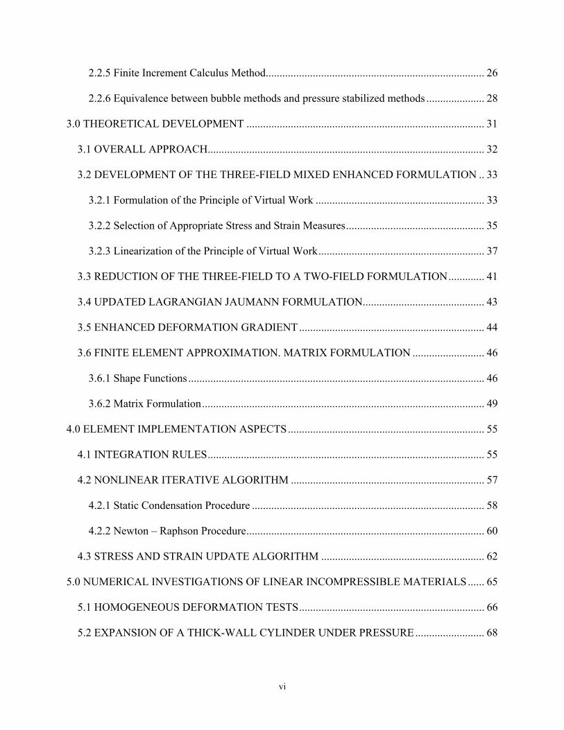
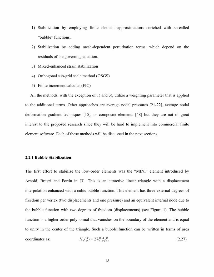
The first effort to stabilize the low–order elements was the “MINI” element introduced by
Arnold, Brezzi and Fortin in [3]. This is an attractive linear triangle with a displacement
interpolation enhanced with a cubic bubble function. This element has three external degrees of
freedom per vertex (two displacements and one pressure) and an equivalent internal node due to
the bubble function with two degrees of freedom (displacements) (see Figure 1). The bubble
function is a higher order polynomial that vanishes on the boundary of the element and is equal
to unity in the center of the triangle. Such a bubble function can be written in terms of area
coordinates as: 32127)( ξξξξ =eN (2.27)
15
Figure 1. Linear displacement/linear pressure triangle with bubble function
The displacement field with the bubble function can be approximated as:
eei
ii uNuN +≈ ∑u (2.28)
where ui are the nodal displacements and ue are internal parameters. Similarly, the pressures are
interpolated as:
∑≈i
ii pNp (2.29)
For the linear triangle and tetrahedral element the shape functions are the area, respectively the
volume coordinates iiN ξ= (2.30)
Because the internal parameters are defined separately for each element, a partial solution can
be performed at the element level to obtain a set of equations in terms of external degrees of
freedom as discussed in the mixed u/p formulation.
Advantages of using bubble function:
- Satisfies LBB condition and the mixed patch test
- Few degrees of freedom
- Easy to implement in large strain deformation because it does not require the introduction
of other parameters
16
Disadvantages:
- Only marginally stable
- This element might not be robust enough since in many tests the pressure solution still
had small amplitude oscillations.
- In transient problems, the accelerations will also involve the bubble mode and will affect
the inertial terms.
2.2.2 Stabilization by Adding Mesh-Dependent Terms
The idea of this method is to modify the discrete equations instead of the interpolation functions.
The simplest form of this type of stabilization is to add a non-zero diagonal term through a
penalty-like term in the pressure constitutive equation. This was first introduced by Brezzi and
Pitkaranta in [11] for stabilizing the finite element approximation of Stokes problem. Numerous
other alternatives of this method have been developed [23-25, 29-30, 43-44]. Recalling from
section 2.1.3, the splitting of the Cauchy stress into the deviatoric and volumetric parts as:
ijijij ps δσ +=+= pIsσ
(2.31)
and noting that the deviatoric stress is related to the deviatoric strain through the relation:
⎟⎟⎠
⎞⎜⎜⎝
⎛∂∂
−∂∂
+∂∂
==k
kij
i
j
j
idevijij x
uxu
xu
GGs δε322 (2.32)
The equilibrium equations in the absence of inertial forces are:
0=+∂∂+
∂∂
iij
ij bxp
xs
(2.33)
Substituting the constitutive equation for the deviatoric part (2.32) into (2.33)
17
031 22
=+∂∂+⎟
⎟⎠
⎞⎜⎜⎝
⎛∂∂
∂+
∂∂∂
iiii
j
ij
i bxp
xxu
xxu
G (2.34)
or in tensor form:
0)(31 2 =+∇+⎟
⎠⎞⎜
⎝⎛ ∇+⋅∇∇ buu pG
where is the Laplacian operator and ∇ is the gradient operator. 2∇
The pressure constitutive equation in terms of displacement is:
Kp
v =⋅∇= uε (2.35)
Taking the divergence of the equilibrium equation (2.34) and using (2.35) we obtain:
0341 2 =⋅∇+∇⎟
⎠⎞⎜
⎝⎛ + bp
KG (2.36)
This equation was used to construct the additional term for the weak form, which would
otherwise be zero. Brezzi and Pitkaranta [11] added a weighted form and set the body force to
zero for simplicity. Then, they integrated by parts and ignored the boundary terms to obtain a
more attractive form of the pressure constitutive equation:
0=∂∂
∂∂+⎟
⎠⎞⎜
⎝⎛ − ∫∫ dV
xp
xpdV
Kpp
iV iV e
δβδ ε1T (2.37)
From dimensional considerations with the first term, the parameter β should have a value
proportional to L4/F where L is length and F is force.
In the work of Hughes et al.[29], β is given in terms of the characteristic element length h and
a non negative, non dimensional stability parameter, α as:
Gh
2
2αβ −= (2.38)
18
This method and alternatives to it have been applied to incompressible linear elasticity and to the
Stokes flow [9-10, 12, 23-25, 29-30, 43]. The above formulation was extended to finite
deformation by O. Klaas et al [31] and applied to a linear displacement, linear pressure
tetrahedral element. They provide a formulation for finite elasticity in both reference and current
configuration, which is then linearized to allow an implementation in a Newton-Raphson
scheme. Their formulation can be used for the hyperelastic materials.
Advantages
- No oscillations in the stress field
- Stress concentrations are well approximated
Disadvantages
- Addition of the non-zero diagonal terms does not have a strong theoretical foundation
- Requires the choice of a parameter
- Depends on the element length (maximum edge length) which also changes under the
large deformation assumption
- Depends also on the material through the shear modulus
2.2.3 Mixed Enhanced Strain Stabilization
This method is presented in Zienkiewicz and Taylor [49] and applied by R. Taylor [47] to a low-
order tetrahedral element in both small deformation and finite deformation. It uses a three-field
approximation involving continuous u, p and discontinuous volume change εv together with an
enhanced strain formulation. The enhanced strains are added to the regular strains to provide the
necessary stabilization for the nearly incompressible case. His formulation starts from the
functional and takes into consideration a hyperelastic material for which a strain energy function
19
exists. This approach though is no longer valid for materials for which we cannot define a strain
energy function.
Small deformation case
Splitting the strain into their deviatoric and volumetric components, the mixed strain can be
written as:
vε1εε dev
31+= (2.39)
The functional, its variation and then linearization are given as:
[ ]
0)()(31
31)(
0)()(31
)1()(),,(
=Π+⎥⎥⎦
⎤
⎢⎢⎣
⎡−+−+⎟
⎠⎞⎜
⎝⎛ +⎟
⎠⎞⎜
⎝⎛ +=Π
=Π+⎥⎥⎦
⎤
⎢⎢⎣
⎡−+−+⎟
⎠⎞⎜
⎝⎛ +=Π
=Π+−+=Π
∫
∫
∫
extV
vvv
T
v
extV
vv
T
v
extV
vT
v
ddVdpddpddd
dVpp
StationarydVpWp
δδεεδεδεδδ
δδεεδδεδδ
εεεεε
δε1ε11εD1ε
δε1ε1σ1ε
TTdevdev
TTdev
Matrix Formulation
The displacement, pressure, and volume change in each element are written using the
interpolation functions in terms of volume coordinates,ξ , and corresponding nodal values as:
(2.40)
vεN
pN
uNuu
ˆˆ)(
ˆˆ)(
ˆˆ)(
==
==
==
αα
αα
αα
εξξε
ξξξξ
vv
pp
Strains are computed using the strain-displacement matrix as: (2.41) αξ u(ξBε α ˆ))( =
An enhanced strain formulation is considered as
eee u(ξBε ˆ))( =ξ (2.42)
where are the enhanced strain parameters and is obtained from the derivatives of a
bubble mode
eu )(ξBe
4321)( ξξξξξ =eN (2.43)
20
Thus, the mixed strain is:
vε1)uBu(BIε eeu
dev
31ˆˆ ++= (2.44)
Replacing all these approximations in the linearized variation of the functional we obtain a linear
system of equations with four unknown increments of displacements, enhanced strain
parameters, pressures and volumetric changes.
The tangent tensor is:
⎥⎥⎥⎥⎥
⎦
⎤
⎢⎢⎢⎢⎢
⎣
⎡
=
vvT
pvT
evT
uv
pvTep
Tup
evepeeT
ue
uvupueuu
KKKKK0KKKKKKKKKK
K (2.45)
dV
dV
dV
dV
dV
vv
pv
v
p
ND11NK
NNK
D1NIBK
1NBK
BDIIBK
e
e
e
e
e
V
TT
V
T
devV
Tuu
V
Tuu
udevdevV
Tuuu
∫
∫
∫
∫
∫
=
−=
=
=
=
91
31 (2.46)
The terms involving the enhanced modes are similar to Kuu , Kup, Kuv but they have Be instead of
Bu.
Finite Elasticity Case
[ ]
0)()(:
)()(
=Π+⎥⎦⎤
⎢⎣⎡ −+−+∂∂=Π
=Π+−+=Π
∫
∫
extV
vv
extV
v
dVpJJpW
StationarydVJpW
δδεεδδδ
ε
δCC
C
(2.47)
21
( )
0)(
)()(:::)(2
=Π+∆−+
+∆−∆+∆+⎥⎦
⎤⎢⎣
⎡∂∂∆+∆
∂∂∂=Π∆
∫
∫ ∫∫
extV
v
V Vv
V
ddVpJ
dVJpdVJpdVWW
δδε
εδδδδδ
δ
CCC
CCC
The tangent terms resulting from the first two integrals can be split into a constitutive part and a
geometric part. The terms involving the enhanced strains will be replaced with the appropriate
terms and will have the same form as those involving regular strains.
( )
dV
dV
dV
JdV
dVpJ
dVpJIIpJ
vvv
pv
v
p
vV v
vv
c
ε
εε
εε
Nσ1D11NK
NNK
NσD1IBK
1NBK
IN1σ131σ:NK
B11σ1σ1311σ1σDIIBK
e
e
e
e
e
V
TTT
V
T
Vdevdev
Tuu
V
Tuu
Tguu
uTTTT
devTdevdevdev
V
Tuuu
∫
∫
∫
∫
∫
∫
⎟⎠⎞⎜
⎝⎛ −=
−=
⎟⎠⎞⎜
⎝⎛ +=
=
⎥⎥⎦
⎤
⎢⎢⎣
⎡⎟⎟⎠
⎞⎜⎜⎝
⎛∇⎟⎟⎠
⎞⎜⎜⎝
⎛−+∇=
⎥⎥⎦
⎤
⎢⎢⎣
⎡⎟⎟⎠
⎞⎜⎜⎝
⎛−−⎟⎟⎠
⎞⎜⎜⎝
⎛−++−=
91
91
32
31
)(
922
32
(2.48)
If the interpolation for u and p is continuous in the whole domain and the volumetric change is
piece wise continuous, the solution can be performed by using static condensation at the element
level. After eliminating ue and εv, a system of equations in incremental nodal displacements and
pressures has to be solved.
Advantages
- Results are free of pressure oscillations
- Enhanced terms are material and mesh independent
- Applies to incompressible elastic, hyperelastic materials and to both small and large
deformations
22
Disadvantages
- Increased computational cost due to the introduction of the additional variables but
compensated by the possibility of performing static condensation
- Behaves poorer in bending than mixed hexahedral elements with discontinuous pressure
and volume change
- Exhibits some locking tendency in bending
2.2.4 Orthogonal Sub-Grid Scale Method
The sub-grid scale approach was proposed first by Hughes [30]. More recently the method of
orthogonal sub-grid scale was introduced by Codina [20] and has been applied to incompressible
fluid dynamics. Chiumenti et al. extended this method to solid mechanics in the context of
incompressible elasticity [19] and J2 plasticity [17-18]. An equal order interpolation is used for
both the displacement and pressure. The basic idea of the method is to decompose the continuous
fields into a coarse component and a fine component, corresponding to different scales. Since the
solution of the problem contains components from both scales it is necessary that the finite
element approximation include the effect of both scales. The coarse scale can be solved by a
standard finite element interpolation, which cannot solve the fine scale. For the problem to be
stable the effect of the fine scale has to be taken into consideration.
Thus, the displacement field can be approximated as;
uuu h~+= (2.49)
and the deviatoric stresses can be split into two corresponding contributions as:
sss h~+= (2.50)
This results in the following mixed formulation in the weak form as:
23
(2.51) ( ) ( ) ( ) ( )
( )( ) 0~
0~~)~(~
=+⋅∇
=++∇+++⋅∇+
∫
∫∫∫dVp
dVpdVdV
V
VVV
uu
buuuussuu
h
hhhh
δδδ
δδδδδδ
which integrated by parts yields three equations of which one is related to the fine scale:
( )( ) ( )( ) ( )( ) ( ) ( )
( )( ) ( ) ( )
( ) ( ) 0~
0~)~(~~
0~
=⋅∇+⋅∇
=+⋅∇+⋅∇
=−−⋅∇+∇+∇
∫∫
∫∫∫
∫∫∫∫∫
dVpdVp
dVdVdV
dVdVdVpdVdV
VV
VVV
VVVV
s
V
s
uu
bususu
tubuususu
h
h
hhhhhh
δδ
δδδ
δδδδδ
(2.52)
The first equation solves the balance of momentum and includes a stabilization term which
depends on the sub-grid stresses. For linear elements this term is zero. The third equation
enforces the incompressibility condition and has a stabilization term that depends on the sub-grid
scale. The second equation is completely defined in the sub-grid scale and cannot be solved by
the finite element mesh. To find the sub-grid displacements that are introduced in the second
stabilization term, Codina proposed to look in the space orthogonal to the finite element space.
Such a method has already been applied with success in fluid mechanics. From the second
equation, it should be noted that these displacements are driven by the residual of the coarse
scale and thus they can be expressed as:
( ))(~ pPp hee ∇−∇= τu (2.53)
where )( pPhh ∇=π is the projection of the gradient of pressure onto the finite element space
and τ e is the same as β from section 2.2.2. Thus the final formulation becomes:
24
( )( ) ( )( ) ( ) ( )
( ) [ ]( )
( )∫
∑∫
∫∫∫∫
=−∇
=−∇⋅∇−⋅∇
=−−⋅∇+∇
=
Vhh
n
ehe
V
VVVV
s
dVp
ppdVp
dVdVdVpdV
elem
0
0
0
1
πδπ
πδτδ
δδδδ
h
hhhhh
u
tubuusu
(2.54)
It is important to note that no stabilization term appears in the first equation for low-order
elements and the only stabilization term appears in the incompressibility equation.
The tangent stiffness matrix is:
(2.55) ⎥⎥⎥
⎦
⎤
⎢⎢⎢
⎣
⎡
−−=
ππττττ
KKKKK
KK
eupe
Tupeppe
Tup
upuu
e
0
0K
Advantages:
- Circumvents the strict LBB condition
- Results are free of volumetric locking and pressure oscillations and comparable
qualitatively to the mixed quadrilateral and hexahedron.
- Correct failure mechanisms with localized patterns of plastic deformations are obtained
which show that the method is not influenced by the mesh directional bias.
Disadvantages:
- The formulation is applicable only for small deformation.
- Requires a parameter depending on element length and shear modulus which makes the
formulation hard to extend to finite deformation case.
- Introduces a new field variable, Πh which is continuous and therefore the static
condensation procedure cannot be performed at element level.
25
2.2.5 Finite Increment Calculus Method
The FIC method is a completely different approach in stabilizing the mixed u/p elements, but
yields the same formulation as the previous discussed method (OSGS). The basis of the FIC
formulation is the satisfaction of the standard equations of equilibrium in a domain of finite size
by expressing the different terms of the differential equation using a Taylor expansion series and
retaining the higher order terms.
The resulting equations are enhanced with some additional terms, which introduce the
necessary stability to overcome the volumetric locking. This method was first developed by
Onate for advective-diffusive and fluid flow problems [33] and was later applied to
incompressible solids in [34-36].
This method allows the use of linear triangle and tetrahedral in quasi-incompressible and fully
incompressible solid problems. For any problem in mechanics, the equations expressing balance
of momentum, mass, heat, etc. can be written in a domain of finite size with h as the
characteristic length. By expanding the balance equation in Taylor expansion and retaining the
lower order term, we get:
02
=∂∂
−k
iki x
rhr (2.56)
where ri is the standard form of the i th differential equation for the infinitesimal problem and hk
is the characteristic length of the domain. This method is not useful for obtaining an analytical
solution but proves to be very useful for finding an approximate solution, which converges to the
analytical one when the grid size tends to zero.
If we consider the mixed u/p formulation as in (2.12) and (2.13) and replacing ri by the
equilibrium equation first and then by the incompressibility equation, we obtain the following:
26
0)(
02
1
=−⎟⎟⎠
⎞⎜⎜⎝
⎛∂∂+−
=∂∂−−−+
∫∫ ∑∫
∫∫∫∫∫
=
dSrnpdVxprdV
Kpp
dVrxuhdStudVbupdVdVs
iiiSV
n
i iii
Vv
iV k
iki
Sii
Vi
Vv
Vijij
d
τδδτεδ
δδδδεδε
(2.57)
where τ i are coefficients referred as intrinsic time parameters with the following value:Ghi
i 83 2
=τ ,
which is very similar with the heuristically value of G
h2
2
=τ chosen in the previous works.
Since the last terms form the first equation and the second equation are not relevant for solid
mechanics problems they are omitted in the final formulation. Also introducing the notation
ij
iji
ii
i
bxs
xpr
+∂∂
=
+∂∂=
π
πwhere (2.58)
π i is the part of the differential equation not containing the pressure gradient This term, once
introduced, has to be weakly enforced by means of a Lagrange multiplier (δπi ) yielding the final
set of governing equations as:
,0
0)(
0
1
=⎟⎟⎠
⎞⎜⎜⎝
⎛+
∂∂
=⎟⎟⎠
⎞⎜⎜⎝
⎛⎥⎦
⎤⎢⎣
⎡+
∂∂
∂∂+−
=−−+
∫
∫ ∑∫
∫∫∫∫
=
dVxp
dVxp
xpdV
Kpp
dStudVbupdVdVs
ii
iV
i
V
n
ii
iii
Vv
iS
iiV
iV
vV
ijij
d
πτδπ
πδτεδ
δδδεδε
(2.59)
Matrix formulation is similar with the one obtained in the OSGS methods.
27
Advantages
- FIC method is based on a very strong theoretical foundation because it emerges naturally
from the governing equations
- Results are accurate and free of pressure oscillations
- Can be used in a simpler form by neglecting the effect of the projected pressure gradient
terms.
- It is applicable to non-linear dynamics.
Disadvantages
- Stabilization parameters are a function of the material properties and characteristic length
- Extension to finite deformation is impeded by the characteristic length parameters whose
consistent definition remains still an open question.
2.2.6 Equivalence between bubble methods and pressure stabilized methods
It can be concluded from the previous sections that the OSGS method produces the same
additional terms in the pressure constitutive equation as FIC method and both results are very
similar with the terms produced by the pressure stabilized methods with the only difference in
the term π, the projected gradient of pressure, which is not so significant for the case of static
analyses. Having established that these three methods are similar, the normal question to ask is
whether the ‘bubble methods’ are equivalent or not to these methods. Answering this question
will lead us immediately to the most efficient and stable method to adopt for our tetrahedral
element. Several authors proved the equivalence between the bubbles and stabilized methods.
Hughes [30] establishes a relationship between ‘bubble function’ methods and stabilized
28
methods and then of both methods to subgrid scale methods. He also identifies the origin of the
τ i parameters that could have never been explained before as being derived from the element
Green’s function. Another equivalence proof is offered by R. Pierre in [38] who has shown that
by eliminating the cubic bubble using static condensation we recover the stabilized methods.
If we write the displacement field as in the OSGS methods:
kKhh uxxuxuxuxu ~)()()(~)()( ∑+=+= φ (2.60)
where uh is an approximation of u
are the internal d.o.f. with corresponding bubble function ϕk. ku~
The next simplifying conditions were used for static condensation:
0)~(:)~(
~)~(:)~(
0)~(:
2211
2
=∇∇
=∇∇
=∇∇
∫
∫
∫Ω
dxuu
uAdxuu
dxuu
kkkkK
kkkkkkK
kkh
φφ
φφ
φ
(2.61)
By replacing (2.60) in the discrete governing equations (equilibrium and constraint) and using
(2.61) we obtain a system of three equations as in the OSGS method out of which the second one
refers only to the internal degrees of freedom or ‘bubble’ parameters. Solving this equation for
the bubble parameters and substituting them in the pressure equation by using a very well known
formula
kK
K hKmeasdx ==∫ )(209φ (2.62)
we get the equivalent form of the pressure equation of the ‘bubble method’ as:
29
0)(
)(
2 =∂∂⋅
∂∂+=
=∂∂⋅
∂∂−−
∫∑∫
∫∫
K iiK
KK
Kv
KK ii
kK
v
dxxp
xphCpdx
dxxp
xphpdx
δδε
φδδε (2.63)
It is easy to observe now the by the process of static condensation and under some conditions the
method of enriching the displacement field with a cubic bubble function produces the same
additional terms in the pressure equation as the pressure stabilized methods. The only difference
is that the ‘bubble methods’ do not produce the projection of pressure gradient that appears in the
OSGS and FIC methods.
Therefore, if all methods are equivalent under certain conditions, it seems natural to choose
the method that would be the most efficient and easiest to implement.
We chose to implement a mixed u/p enhanced strain approach with the enhanced strain
derived from a bubble function for the following reasons:
– Reasonably stable
– Consistent in nonlinear (large deformation) analysis
– No material or mesh dependent parameters
– Computationally efficient (less degrees of freedom per element).
30
3.0 THEORETICAL DEVELOPMENT
In the present work, a mixed enhanced strain formulation is introduced for a lower-order
tetrahedral solid element that is applicable to small and large deformations and large rotations.
The uniqueness of the formulation lies within the fact that no specific geometric or material
model parameters are required and no specific material model is chosen which makes the
formulation as general as possible. The theoretical formulation is developed from the principle of
virtual work and it has a three-field form. The proposed element has a node in each corner with
displacement and pressure as external degrees of freedom and a center node with the volumetric
strain and displacement as internal degrees of freedom. The stabilization term comes from an
enhanced strain derived from a bubble function. Two bubble functions, conforming and
nonconforming, are studied for obtaining optimal results. Two formulations, a general three-field
formulation and its reduction to a two-field form are presented in the next sections. For
efficiency reasons, the reduced two-field form was implemented through a user-programmable
element into the commercial finite element software, ANSYS.
31
3.1 OVERALL APPROACH
Since the proposed formulation is applicable to general finite strain deformation, it has to take
into consideration the following factors [6]:
• Geometry changes during deformation; the current configuration is different from the
reference configuration and different from the configurations at any other time.
• A large strain definition has to be used.
• Cauchy stress cannot be updated by simply adding its increment due to straining of the
material. Cauchy stresses at time t+∆t have to take into account the rigid body rotations.
• Implementation of the non-linear behavior should be based on an incremental approach.
• The equilibrium of the body must be established in the current configuration.
The basic idea of the nonlinear finite element formulation is to linearize the weak form of the
governing equations of the problem and to solve these equations for the finite elements
discretized domain. This leads to an incremental approach, according to which the solution at
each step is obtained from the solution at the previous step. A step is considered a load increment
in a static analysis and a time step in transient analysis.
The proposed three-field formulation follows the mixed enhanced strain formulation of Taylor
[47] with the difference that it starts from the weak form instead of an energy functional ( the
weak form is more general-it applies to problems that don’t have a variational principle) and uses
the Jaumann rate of Cauchy stress with its conjugate deformation rate instead of second Piola-
Kirchhoff stress conjugated with Green-Lagrange strain. In his formulations for both small and
large deformation problems it is assumed that there exists a stored energy function for the
material, expressed in terms of the right Green deformation tensor, which is not always the case.
32
The present formulation does not assume the existence of such a function but employs a rate
form of the constitutive equation which is suitable for both rate-dependent and rate-independent
material constitutive laws. This is due to the fact that the Jaumann rate of Cauchy stress is
employed as an objective stress rate in the constitutive law. An Updated Lagrangian Jaumann
(ULJ) procedure is employed to solve for geometric nonlinearities because of its ability to handle
large displacements, large rotations, and large strain analyses. For the finite element
implementation, a similar approach to Bathe [6] will be used.
3.2 DEVELOPMENT OF THE THREE-FIELD MIXED ENHANCED FORMULATION
3.2.1 Formulation of the Principle of Virtual Work
Formulating the principle of virtual work constitutes the basis of the theoretical development
since obtaining the set of linearized equations is the main goal of an element formulation. They
are obtained by differentiating the principle of virtual work and retaining only the linear terms
(all higher order terms are ignored). The principle of virtual work, which is the weak form of the
equations of equilibrium, is used as the basic equilibrium statement for the proposed formulation
[16]. This weak form expresses the equilibrium state in the form of an integral over the entire
volume of the body and provides a stronger mathematical basis for studying the approximation
than directly discretizing the differential equations of equilibrium and requiring them to be
satisfied point wise.
Since the first formulation has three independent variables, displacement, pressure and
volumetric strain, the Cauchy stresses have to be modified with the corresponding independent
33
pressure field and the strains have to be modified with the corresponding independent volumetric
strain as [2]:
)( PPPPP ijijijijijijdevijij −+=+−=+= δσδδσδσσ (3.1)
)(31
31
, venhvij
enhijv
enhij
enhdevij
enhij εεδεεδεε −−=+= (3.2)
where ijσ is the Cauchy stress from constitutive law,
devijσ is the deviatoric part of the Cauchy stress,
P is the pressure derived from Cauchy stress,
P is the interpolated pressure,
enhijε is the modified enhanced strain with the stabilizing term from the bubble function
devijε is the deviatoric part of the strain,
vε is the interpolated volumetric strain and
ijδ is the Kronecker delta.
The internal virtual work can be expressed now as:
dVW enhij
V
enhijij δεεσδ ∫= )(int (3.3)
The two constraints imposed by the two additional variables are:
0=− vv εε (3.4)
0=− PP (3.5)
The introduction of the two additional field variables has to be weakly enforced in the principle
of virtual work by means of two Lagrange multipliers as:
dVPPdVPdVW vV
enhv
Vv
enhv
enhij
enhij
Vij εδεδεεδεεσδ ))(()()(int −+−+= ∫∫∫ (3.6)
34
The augmented principle of virtual work is differentiated again to obtain the incremental
principle of virtual work, which yields, by substituting the variables with their finite element
approximations, the matrix formulation or the linearized system of equations that has to be
solved. During the differentiation process we will obtain the rates of the Cauchy stress and of
strains and therefore we need to appropriately define them. This is done in the next section.
3.2.2 Selection of Appropriate Stress and Strain Measures
When a small strain approximation is no longer valid we have to use appropriate measures of
stress and strain. The approach that we will follow is to use stress and strain measures that are
conjugate so that the principle of virtual work can be expressed as in (3.6).
Many of the materials we wish to model are history dependent and therefore it is common for
the constitutive equations to appear in rate form. We therefore need to define the rate of the
Cauchy stress for use in the material constitutive law which relates the increments of stress with
the increments of strain. One of the objective stresses that can be applied is the Jaumann rate of
Cauchy stress expressed by McMeeking and Rice in [32].
The issue that arises when using the second Piola - Kirchhoff stress, which is a materially-
based stress, is that it remains constant during the rotation because its components are associated
with a material basis. The problem is that the components of the Cauchy stress,σ, are associated
with the current directions in space and, therefore, the Cauchy stress rate, Dσ, will be nonzero if
there is pure rigid body rotation even though from a constitutive point of view the material is
unchanged. Thus, the increment of Cauchy stress, Dσ, must be divided into two different parts:
one due to the rigid body motion only and one associated to the rate form of the stress-strain law.
35
According to [1], if at time t we attach to a material point a set of base vectors, ei, i=1, 2, 3
they cannot stretch but they can spin with the same spin as the material,
⎟⎟⎠
⎞⎜⎜⎝
⎛∂∂−
∂∂=
T
xv
xvΩ
21 (3.7)
Therefore, their motion can be described as:
eΩe ⋅=& (3.8)
Thus, if we consider the Cauchy stress tensor in the current configuration as
jiij eeσ=σ (3.9)
Taking the time derivative we obtain:
)Ωσσ(Ωσσ TJ ⋅+⋅+= && (3.10)
where is the rate of Cauchy stress associated with the constitutive response, also called the
Jaumann rate of Cauchy stress. The Jaumann stress rate is an objective stress rate tensor that is
related to the rate of straining as:
Jσ&
klijklklijklJij dCDC == εσ.
(3.11)
with as the components of material constitutive tensor, ijklC
⎟⎟⎠
⎞⎜⎜⎝
⎛∂∂
+∂∂
==k
l
l
kklkl x
vxv
dD21ε as the components of the rate of deformation tensor,
and is the velocity. iv
Since the Jaumann stress rate is defined in terms of both rate of deformation and past history
this equation provides a link between the material model and the overall change in Cauchy stress.
Written in indicial notation [28],
ikjkjkikijJij ωσωσσσ &&&& −−= where (3.12)
36

⎟⎟⎠
⎞⎜⎜⎝
⎛∂∂
−∂∂
=i
j
j
iij x
vxv
21ω& is the spin tensor defined in (3.7) written in indicial notation and
ijσ& is the time rate of Cauchy stress.
Then the Cauchy stress rate becomes:
ikjkjkikklijklij DDDCD ωσωσεσ ++= (3.13)
where ⎟⎟⎠
⎞⎜⎜⎝
⎛∂∂
−∂∂
=i
j
j
iij x
uxu
21ω are the components of the rotation tensor.
This means that an integration process is always required to evaluate the Cauchy stresses. Thus is
suitable for an analysis of path-dependent materials [32].
Under these circumstances the differentiated or linearized principle of virtual work with
respect to the current configuration can be used to formulate the Updated Lagrangian Jaumann
finite element method. The complete derivation of the differentiation process is presented in the
next section and Appendix A.
3.2.3 Linearization of the Principle of Virtual Work
Using the augmented internal virtual work from (3.6) we can formulate the principle of virtual
work as: (3.14)
0))(()()(int =+−+−+=+= ∫∫∫ extvV
enhv
Vv
enhv
enhij
enhij
Vijext WdVPPdVPdVWWW δεδεδεεδεεσδδδ
Taking the derivative with respect to time of the internal virtual work we get:
( ) ( )( ) ( ) dVPDDPdVPPD
dVPDdVPDDdVDdVDWD
vVV
v
Vv
enhv
Vv
enhv
enhij
Vij
enhij
Vij
εδεδ
δεεδεεδεσδεσδ
∫∫
∫∫∫∫−+−+
+−+−++=int
(3.15)
37
where the differentiation of dVDdVx
DudVD v
k
k ε=∂∂
=)( . This term is usually insignificant in
most deformation cases and is ignored. Also this term will yield an unsymmetrical stiffness
matrix [2]. The same observations can be made for the terms involving vDPD εδδ , which are
very small and can be ignored.
After making these simplifying assumptions, the linearized augmented principle of virtual
work becomes:
DdVPD
dVCdVDWD
VV
enhv
vijklV
enhij
Vijij
Vija
∫∫
∫∫∫−+
++=
εδε
εδδεσδ )31 enh
klijδ(dVD enhδεσ (3.16)
Extending the first two
Jaumann stress rate from
dVDC
dVDC
dVD
DC
DDC
dVDA
vklijklV
enhij
V
enhklijkl
V
enhij
V
env
V
enhijij
enhijijkl
V
enhij
ikenhkl
Vijkl
V
enhij
Vij
∫
∫
∫∫
∫
∫
∫∫
+
−=
++
⎢⎣⎡ −=
+=
+=
εδδε
εδε
δεδεσ
δεδε
ωσε
σδεσ
31
31
[
A
+
dVPDdVPV
vv ∫− εδδ
integrals, which are grouped
(3.13) we obtain:
( ) (
[
DC
dVDC
dVDCPD
dVDD
DPPDD
dVD
Vkl
enhklijklij
enhv
V
ei
enhvklijkl
enhij
enhijijklij
h
V
enhijv
enhvkl
ijikjkjk
enhijij
∫
∫∫
∫
−−
+
=⎟⎠⎞⎜
⎝⎛ −
+⎥⎦⎤−
−++
=
δεδδε
δεεδδε
εδ
σδεεε
δδωσ
δε
31[
3131
31
)](
38
B Dε
as term A, and using the definition of
)
( ) ]
dVPDdV
dVDDD
dVDD
dVD
V
enhvv
enhv
enhijijikjkjkik
nhj
ikjkjkik
enhijij
enhij
∫+−
+++
++
=+
δεεε
δεσωσωσ
ωσω
δεσε
)](
( )[ ]
dVPDdVDCdVDC
dVDDD
dVDC
dVDCdVDCdVDCA
V
enhv
Vvklijklij
enhvvklijkl
V
enhij
V
enhijijikjkjkik
enhij
enhvkl
Vijklij
enhv
enhklijklij
V
enhv
enhvklijkl
V
enhij
enhklijkl
V
enhij
∫∫∫
∫
∫
∫∫∫
+−+
++++
++
+−−=
δεεδδδεεδδε
δεσωσωσδε
εδδδε
εδδεεδδεεδε
31
31
31
31
31
31
31
(3.17)
The first four integrals in (3.17) produce the so-called constitutive stiffness term, , because it
comes from the material constitutive law directly or from the straining; the fifth integral which
will be extended in the next section produces the so-called stress stiffness term or geometric
stiffness, (due to geometric nonlinearities).
cuuK
geomuuK
∫ ∫∫
∫
∫
+−=
=−−=
==
Vv
Vklijklijv
enhvkl
Vijklijv
enhklijklijv
Vv
enhvkl
enhklijklijv
venhklijklij
V
dVDCdVDCdVDC
dVDC
dVDCB
εδδεδεδδεδεδεδ
εεδεδεδ
εδεδ
31
31
31
31
31
)](31[
31
)31(
(3.18)
Rewriting (3.16) using the obtained formulas for terms A and B we get the linearized principle of
virtual work as:
( )[ ]
dVPDdVPDdVPD
dVDCdVDCdVDC
dVPDdVDCdVDC
dVDDD
dVDC
dVDCdVDCdVDCWD
Vv
Vv
V
enhv
Vv
Vklijklijv
enhvkl
Vijklijv
enhklijklijv
V
enhv
Vvklijklij
enhvvklijkl
V
enhij
V
enhijijikjkjkik
enhij
enhvkl
Vijklij
enhv
enhklijklij
V
enhv
enhvklijkl
V
enhij
enhklijkl
V
enhija
∫∫∫
∫ ∫∫
∫∫∫
∫
∫
∫∫∫
−−+
++−+
++−+
++++
++
+−−=
εδδεδε
εδδεδεδδεδεδεδ
δεεδδδεεδδε
δεσωσωσδε
εδδδε
εδδεεδδεεδεδ
31
31
31
31
31
31
31
31
31
31
31
31
(3.19)
39
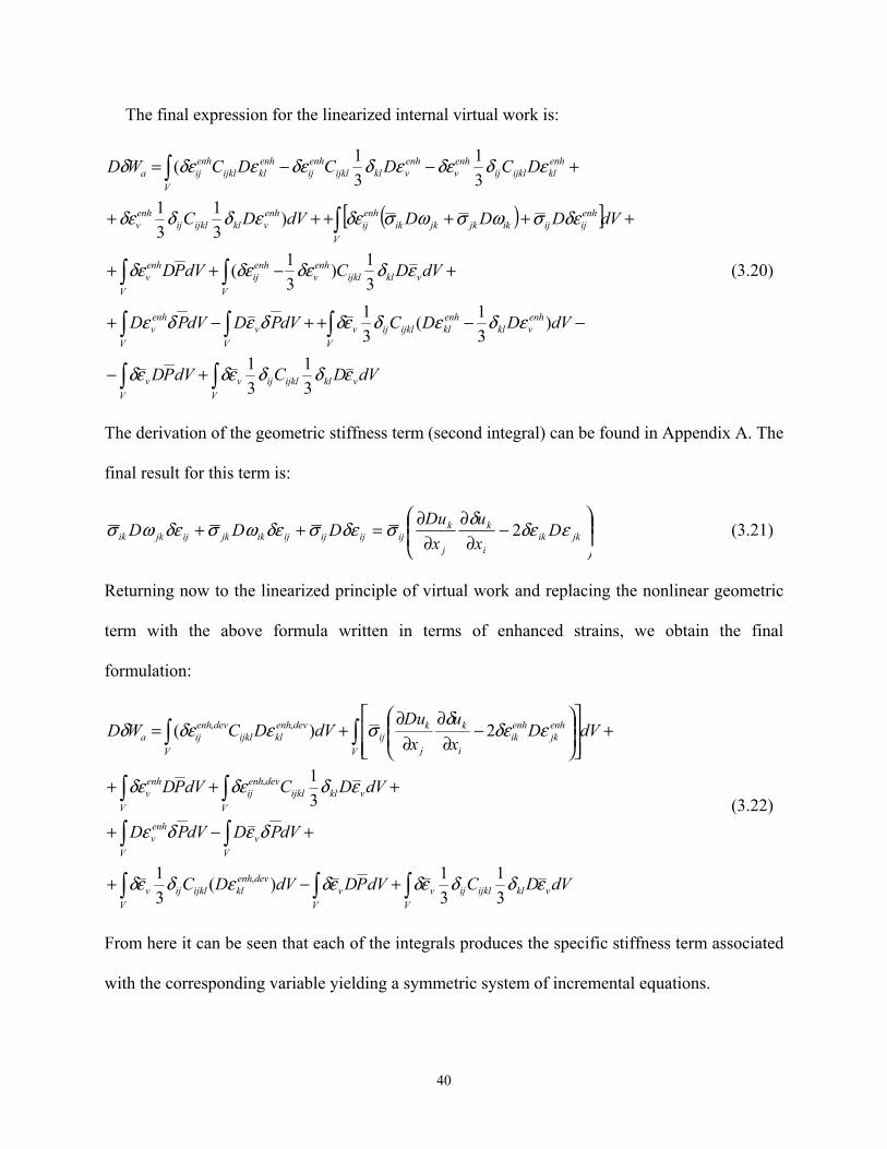
The final expression for the linearized internal virtual work is:
( )[ ]
dVDCdVPD
dVDDCdVPDdVPD
dVDCdVPD
dVDDDdVDC
DCDCDCWD
vV
klijklijvV
v
V
enhvkl
enhklijklijv
Vv
V
enhv
vklijklenhv
V
enhij
V
enhv
V
enhijijikjkjkik
enhij
enhvklijklij
enhv
enhklijklij
enhv
enhvklijkl
enhij
enhklijkl
V
enhija
εδδεδεδ
εδεδεδδεδε
εδδεδεδε
δεσωσωσδεεδδδε
εδδεεδδεεδεδ
∫∫
∫∫∫
∫∫
∫
∫
+−
−−++−+
+−++
++++++
+−−=
31
31
)31(
3131)
31(
)31
31
31
31(
(3.20)
The derivation of the geometric stiffness term (second integral) can be found in Appendix A. The
final result for this term is:
⎟⎟⎠
⎞⎜⎜⎝
⎛−
∂∂
∂∂
=++ jkiki
k
j
kijijijijikjkijjkik D
xu
xDu
DDD εδεδσδεσδεωσδεωσ 2 (3.21)
Returning now to the linearized principle of virtual work and replacing the nonlinear geometric
term with the above formula written in terms of enhanced strains, we obtain the final
formulation:
dVDCdVPDdVDC
dVPDdVPD
dVDCdVPD
dVDxu
xDu
dVDCWD
vV
klijklijvV
vV
devenhklijklijv
Vv
V
enhv
vklijklV
devenhij
V
enhv
V
enhjk
enhik
i
k
j
kij
devenhklijkl
V
devenhija
εδδεδεδεδεδ
δεδε
εδδεδε
εδεδσεδεδ
∫∫∫
∫∫
∫∫
∫∫
+−+
+−+
+++
+⎥⎥⎦
⎤
⎢⎢⎣
⎡⎟⎟⎠
⎞⎜⎜⎝
⎛−
∂∂
∂∂
+=
31
31)(
31
31
2)(
,
,
,,
(3.22)
From here it can be seen that each of the integrals produces the specific stiffness term associated
with the corresponding variable yielding a symmetric system of incremental equations.
40
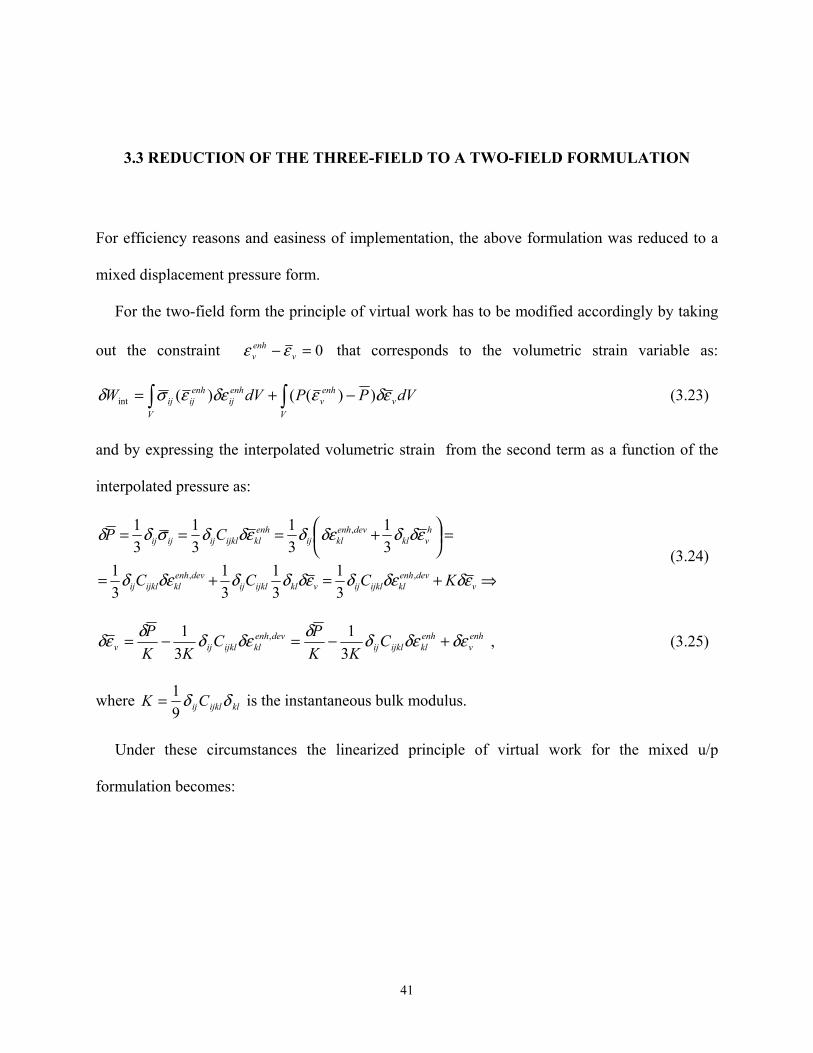
3.3 REDUCTION OF THE THREE-FIELD TO A TWO-FIELD FORMULATION
For efficiency reasons and easiness of implementation, the above formulation was reduced to a
mixed displacement pressure form.
For the two-field form the principle of virtual work has to be modified accordingly by taking
out the constraint 0=− venhv εε that corresponds to the volumetric strain variable as:
dVPPdVW vV
enhv
enhij
enhij
Vij εδεδεεσδ ))(()(int −+= ∫∫ (3.23)
and by expressing the interpolated volumetric strain from the second term as a function of the
interpolated pressure as:
⇒+=+=
=⎟⎠⎞⎜
⎝⎛ +===
vdevenh
klijklijvklijklijdevenh
klijklij
hvkl
devenhklij
enhklijklijijij
KCCC
CP
εδδεδεδδδδεδ
εδδδεδεδδσδδ
,,
,
31
31
31
31
31
31
31
31
(3.24)
enhv
enhklijklij
devenhklijklijv C
KKPC
KKP δεδεδδδεδδεδ +−=−=
31
31 , , (3.25)
where klijklijCK δδ91= is the instantaneous bulk modulus.
Under these circumstances the linearized principle of virtual work for the mixed u/p
formulation becomes:
41
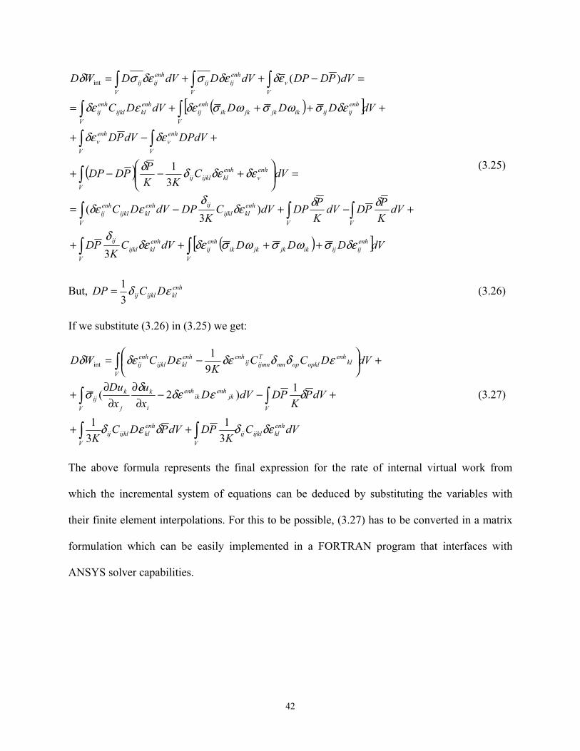
( )[ ]
( )
( )[ ]dVDDDdVCK
PD
dVKPPDdV
KPDPdVC
KDPdVDC
dVCKK
PPDDP
DPdVdVPD
dVDDDdVDC
dVPDDPdVDdVDWD
V
enhijijikjkjkik
enhij
V
enhklijkl
ij
VV
enhklijkl
ijenhkl
Vijkl
enhij
enhv
enhklijklij
V
V
enhv
V
enhv
V
enhijijikjkjkik
enhij
enhkl
Vijkl
enhij
Vv
enhij
Vij
enhij
Vij
∫∫
∫∫∫
∫
∫∫
∫∫
∫∫∫
++++
+−+−=
=⎟⎟⎠
⎞⎜⎜⎝
⎛ +−−+
+−+
++++=
=−++=
δεσωσωσδεδεδ
δδδεδ
εδε
δεδεδδ
δεδε
δεσωσωσδεεδε
εδδεσδεσδ
3
)3
(
31
)(int
(3.25)
But, enhklijklij DCDP εδ
31= (3.26)
If we substitute (3.26) in (3.25) we get:
dVCK
PDdVPDCK
dVPK
PDdVDxu
xDu
dVDCCK
DCWD
enhklijklij
V
enhklijklij
V
V
jkenh
ikenh
i
k
V j
kij
V
klenh
opklopmnTijmnij
enhenhklijkl
enhij
δεδδεδ
δεδεδσ
εδδδεεδεδ
∫∫
∫∫
∫
++
+−−∂∂
∂∂
+
+⎟⎠⎞⎜
⎝⎛ −=
31
31
1)2(
91
int
(3.27)
The above formula represents the final expression for the rate of internal virtual work from
which the incremental system of equations can be deduced by substituting the variables with
their finite element interpolations. For this to be possible, (3.27) has to be converted in a matrix
formulation which can be easily implemented in a FORTRAN program that interfaces with
ANSYS solver capabilities.
42
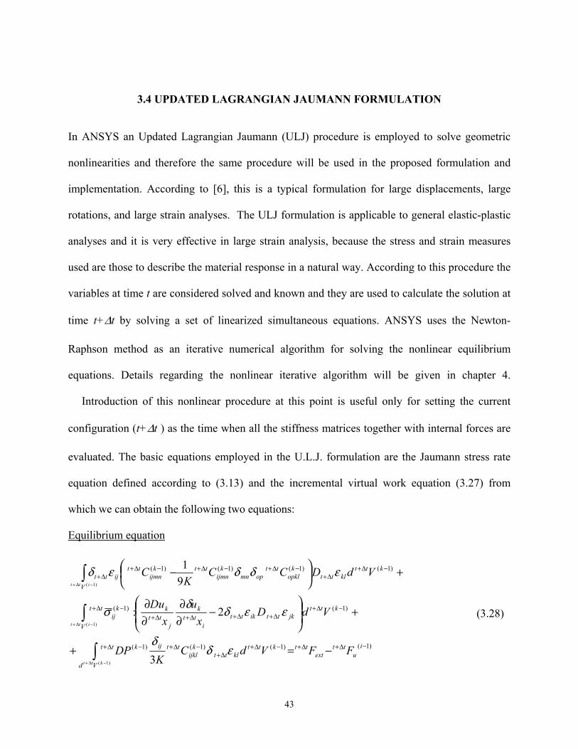
3.4 UPDATED LAGRANGIAN JAUMANN FORMULATION
In ANSYS an Updated Lagrangian Jaumann (ULJ) procedure is employed to solve geometric
nonlinearities and therefore the same procedure will be used in the proposed formulation and
implementation. According to [6], this is a typical formulation for large displacements, large
rotations, and large strain analyses. The ULJ formulation is applicable to general elastic-plastic
analyses and it is very effective in large strain analysis, because the stress and strain measures
used are those to describe the material response in a natural way. According to this procedure the
variables at time t are considered solved and known and they are used to calculate the solution at
time t+∆t by solving a set of linearized simultaneous equations. ANSYS uses the Newton-
Raphson method as an iterative numerical algorithm for solving the nonlinear equilibrium
equations. Details regarding the nonlinear iterative algorithm will be given in chapter 4.
Introduction of this nonlinear procedure at this point is useful only for setting the current
configuration (t+∆t ) as the time when all the stiffness matrices together with internal forces are
evaluated. The basic equations employed in the U.L.J. formulation are the Jaumann stress rate
equation defined according to (3.13) and the incremental virtual work equation (3.27) from
which we can obtain the following two equations:
Equilibrium equation
)1()1()1()1(
)1()1(
)1()1()1()1(
3
2:
91
)1(
)1(
)1(
−∆+∆+−∆+∆+
−∆+−∆+
−∆+∆+∆+∆+∆+
−∆+
−∆+∆+
−∆+−∆+−∆+∆+
−=+
+⎟⎟⎠
⎞⎜⎜⎝
⎛−
∂∂
∂∂
+⎟⎠⎞⎜
⎝⎛ −
∫
∫
∫
−∆+
−∆+
−∆+
iu
ttext
ttkttkltt
kijkl
ttij
Vd
ktt
kttjkttiktt
ittk
jtt
k
V
kij
tt
kttkltt
kopkl
ttopmn
kijmn
ttkijmn
ttij
Vtt
FFVdCK
DP
VdDx
ux
Du
VdDCCK
C
ktt
itt
itt
εδδ
εεδδσ
εδδεδ
(3.28)
43
Constraint Equation
)1()1()1()1( 013 )1()1(
−∆+−∆+∆+
∆+−∆+∆+∆+
−∆+ −=− ∫∫−∆+−∆+
kp
ttktttt
Vd
ttkttttkltt
kijkl
ttij
V
FVdPK
PDVdPDCK kttktt
δδεδ
(3.29)
where is the incremental material property tensor at time t+∆t, referred to the
configuration at time t+∆t ;
)1( −∆+ kijkl
tt C
)1( −∆+ kij
tt σ is the modified Cauchy stress at time t+∆t; and
and
ijtt Dε∆+
PDtt ∆+ are the incremental strains and pressures which are referred to the configuration at
time t+∆t. All the quantities with (k-1) superscript mean that they are evaluated at t+∆t using the
value of the displacements obtained from the previous iteration.
Since we are interested in finding the solution in current configuration in terms of the solution
of previous configuration the key term that will provide this is the deformation gradient tensor.
3.5 ENHANCED DEFORMATION GRADIENT
In most structural problems we are interested in finding the deformation of the structure
throughout the loading history in terms of a reference configuration that is given. Suppose a
particle is located at position X initially and moves to position x. The location of the particle in
current configuration is related to the location in the reference configuration by the displacement
u and is given by:
uXx += (3.30)
The deformation gradient matrix is defined as:
( )XuI
XuX
XxF
∂∂+=
∂+∂=
∂∂= (3.31)
44
Since the proposed formulation is based on enhancing the deformation mode such that it will
prevent volumetric locking it is necessary to relate this deformation mode to a modification of
the deformation gradient. This approach has been applied successfully by Taylor [47] to
tetrahedral elements.
The incremental deformation gradient can expressed as:
⎥⎥⎥⎥⎥⎥⎥
⎦
⎤
⎢⎢⎢⎢⎢⎢⎢
⎣
⎡
∂∂
∂∂
∂∂
∂∂
∂∂
∂∂
∂∂
∂∂
∂∂
==∆
∆+∆+∆+
∆+∆+∆+
∆+∆+∆+
∆+
3
3
2
3
1
3
3
2
2
2
1
2
3
1
2
1
1
1
xx
xx
xx
xx
xx
xx
xx
xx
xx
FF
t
tt
t
tt
t
tt
t
tt
t
tt
t
tt
t
tt
t
tt
t
tt
ttt (3.32)
or in indicial notation
( )j
ti
ijj
tii
t
jt
itt
ijx
DuxDux
xxF
∂∂+=
∂+∂=
∂∂=∆
∆+
δ (3.33)
The enhanced deformation gradient is enhanced with a term, F∆ , obtained from the derivatives
of the bubble function as:
ijijenh
ij FFF ∆+∆=∆ (3.34)
The total enhanced deformation gradient from the initial configuration to the current
configuration is computed in terms of deformation gradient at previous time step and incremental
deformation gradient as:
enhtenhttt
enhtt FFF 00 ⋅∆= ∆+∆+ (3.35)
The volume has to be modified consistently as:
tenhenhtttt dVFdVFdV ⋅∆== ∆+∆+ 00 (3.36)
45
3.6 FINITE ELEMENT APPROXIMATION. MATRIX FORMULATION
The finite element approximation for the developed formulation is based on assuming a linear
interpolation for both the displacement and pressure fields. Generally, the interpolation can be
written as:
ααaNa = (3.37)
where a is a vector-valued function at any point; Nα is a set of interpolation functions also called
shape functions and aα is a set of nodal variables.
If we use an isoparametric concept for our four-node tetrahedral element then the coordinates
of any point in the tetrahedron can be expressed as:
Nxx(ξNx4
1α
αα == ∑=
) (3.38)
and the same shape functions are used to define the displacement and pressure variables as:
PNN
NuuNu
==
==
∑
∑
=
=
α
α
α
α
α
α
ξξ
ξξ
PP4
1
4
1
)()(
)()( (3.39)
3.6.1 Shape Functions
The 4-node tetrahedral element is defined by a set of volume coordinates, ξ 1, ξ 2, ξ 3, ξ 4 which
represent the ratio of the shaded volume to the total volume (see Figure 2)
46
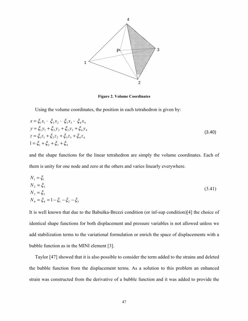
4
3 P
1
Figure 2.
Using the volume coordinates, the positi
4321
44332211
44332211
44332211
1 ξξξξξξξξξξξξξξξξ
+++=+++=+++=+++=
zzzzzyyyyy
xxxxx
and the shape functions for the linear tetra
them is unity for one node and zero at the o
32144
33
22
11
1 ξξξξξξξ
−−−=====
NNNN
It is well known that due to the Babuška-B
identical shape functions for both displacem
add stabilization terms to the variational fo
bubble function as in the MINI element [3].
Taylor [47] showed that it is also possibl
the bubble function from the displacemen
strain was constructed from the derivative
2
Volume Coordinates
on in each tetrahedron is given by:
(3.40)
hedron are simply the volume coordinates. Each of
thers and varies linearly everywhere.
(3.41)
rezzi condition (or inf-sup condition)[4] the choice of
ent and pressure variables is not allowed unless we
rmulation or enrich the space of displacements with a
e to consider the term added to the strains and deleted
t terms. As a solution to this problem an enhanced
of a bubble function and it was added to provide the
47
necessary stabilization. Our element is based on the same approach and therefore it will have a
node in each corner and an internal node located in the center. Two bubble functions,
conforming and nonconforming, are studied for an optimal selection.
Conforming Bubble Functions
These functions are a family of high order polynomials that are zero on the boundary of the
element. A standard conforming bubble function is the cubic bubble function. The cubic bubble
function was used in the development of MINI element and also in the available literature related
to triangular and tetrahedral elements [5, 9-10, 12, 23-25, 29-30]. If, for any tetrahedral element
we denote the volumetric coordinates by ξ i, i=1,2,3,4, the conforming bubbles are according to
[39]:
)1(64 321321 ξξξξξξ −−−=ceN (3.42)
This bubble function was used by Taylor [47] in the formulation of his mixed-enhanced
tetrahedral element. Taylor’s results indicate that the conforming bubble function in (3.52) does
not eliminate all oscillations for problems where strong pressure gradients occur. Accordingly, in
this research, we will also consider other choice for bubble functions.
Non-Conforming Bubble Functions
R. Pierre showed in 1995 [39], that the conforming bubbles satisfy the LBB condition as long
as the mesh is regular. He demonstrated that this happens only if the triangle is equilateral.
Hence, he proposed an optimal bubble function for which the local stabilizing effect is the
greatest.
This optimal bubble function is a quadratic non-conforming one which means that it does not
vanish on the perimeter but it is unity in the center node. This function is defined for any
tetrahedron as:
48
∑=
−=4
1
242i
iqeN ξ (3.43)
This function was also used in our formulation due to the following advantages:
• It has the highest stabilizing factor, especially in three dimensions..
• Since it is a quadratic function it will yield linear strains which are fully consistent with
the linear interpolations of u and p.
• Implies a lower computational cost due to the fact that we use a quadratic function
instead of a cubic (2D) or a quartic one (3D).
• Numerical integration is also less costly.
• In every other aspect the nonconforming bubble is as simple to use as the conforming
one.
3.6.2 Matrix Formulation
Using the same interpolation functions for all variables, the displacements and pressures can be
represented as:
αα
αα
αα
αα
αα
αα
ξξξξδξξδδξξδ
ξξξξ
PDPDDD
PP
PP
==
==
==
)(,)(
)(,)(
)(,)(
uu
uu
uu (3.44)
where the nodal displacements and pressures together with their variations and increments are:
[ ] [ ][ ] [ ][ ] [ ]T
T
T
Puuuuu
Pδuuuuu
Puuuuu
43214321
43214321
43214321
,
,
,
PDPDPDPDDDDDDD
PδPδPδPδ
PPPP
T
T
T
==
==
==
αα
αα
αα
δδδδδ (3.45)
49
and the discretized strains are expressed with the help of an enhanced strain-displacement matrix
Benh as :
αα
αα
αα
δδuBε
uBε
uBε
DD enhenh
enhenh
enhenh
≈
≈
≈
(3.46)
The enlarged strain-displacement matrix has three additional columns corresponding to the three
additional internal displacements and it has to be evaluated with respect to the current
configuration. It has the form: (3.47)
⎥⎥⎥⎥⎥⎥⎥⎥⎥⎥⎥⎥⎥⎥⎥
⎦
⎤
⎢⎢⎢⎢⎢⎢⎢⎢⎢⎢⎢⎢⎢⎢⎢
⎣
⎡
∂∂
∂∂
=∂∂
∂∂
∂∂
∂∂
∂∂
∂∂
∂∂
∂∂
∂∂
∂∂
∂∂
∂∂
∂∂
∂∂
∂∂
∂∂
=
∆+∆+∆+∆+
∆+∆+∆+∆+
∆+∆+∆+∆+
∆+∆+
∆+∆+
∆+∆+
∆+
131
1
3
1
232
1
3
1
121
1
2
1
33
1
22
1
11
1
04,10
00
00
0000
0000
0000
xN
xN
xN
xN
xN
xN
xN
xN
xN
xN
xN
xN
xN
xN
xN
xN
xN
xN
B
tte
tte
tttt
tte
tte
tttt
tte
tte
tttt
tte
tt
tte
tt
tte
tt
enhtt
α
Evaluation of the Cartesian derivatives of the shape functions at time t+∆t can be done using the
derivatives at time t and incremental deformation gradient defined in (3.32):
jt
Tenhkj
ttt
jtt
enhkj
ttt
ktt
jt
ktt
ktt
jt x
NF
xN
Fx
Nxx
xN
xN
∂∂⋅∆=
∂∂
⇒∆⋅∂∂
=∂∂⋅
∂∂
=∂∂ −∆+
∆+∆+
∆+
∆+
∆+ααααα )()( (3.48)
Using the above finite element approximations and by placing the variations in the left hand
side and the increments in the right hand side, each of the integrals from (3.27) yields the
specific stiffness matrix associated with the corresponding variable as:
50
1. Constitutive stiffness matrix:
dVK enh
T
Venh
cenhuu C)BIIC(CBK T ⋅⋅⋅−= ∫ 9
1, (3.49)
2. Displacement pressure stiffness matrices:
dVK enht
V
enhpu
enhup NICB)(KK TTT ⋅⋅== ∫ 3
1 (3.50)
3. Pressure stiffness matrix:
dVKV
pp NNK T ⋅−= ∫1 (3.51)
where the Voigt matrix notation was used (each second rank tensor is written as a vector and
each fourth rank tensor as a matrix).
According to this notation we have:
[ Tzxyzxyzzyyxx σσσσσσ=σ ]
]
]
(3.52)
[ Tzxyzxyzzyyxx εεεεεε 222=ε (3.53)
[ T000111=I (3.54)
The elastic moduli are written also in terms of a matrix as:
⎥⎥⎥⎥⎥⎥⎥⎥
⎦
⎤
⎢⎢⎢⎢⎢⎢⎢⎢
⎣
⎡
=
666564636261
565554535251
464544434241
363534333131
262524232221
161514131211
CCCCCCCCCCCCCCCCCCCCCCCCCCCCCCCCCCCC
C (3.55)
When large deformations are expected the geometric stiffness matrix is added to the
constitutive stiffness matrix to form the final stiffness matrix which is a square symmetric matrix
having the dimension of the total number of degrees of freedom.
51
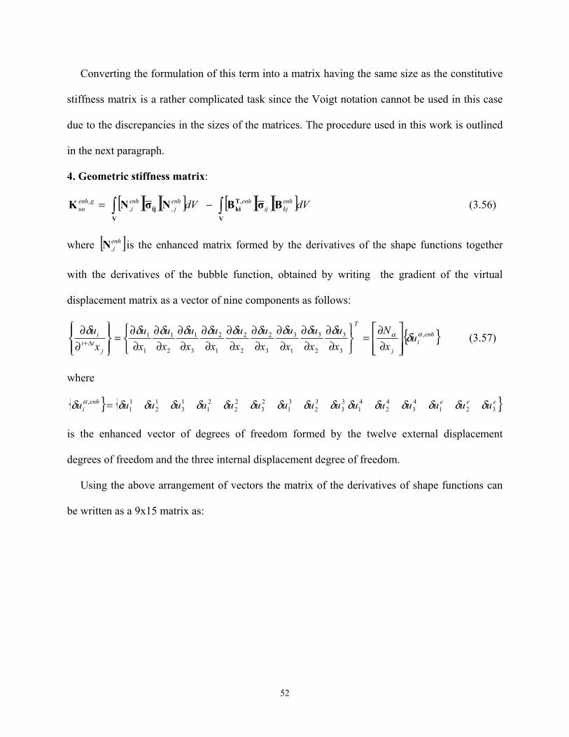
Converting the formulation of this term into a matrix having the same size as the constitutive
stiffness matrix is a rather complicated task since the Voigt notation cannot be used in this case
due to the discrepancies in the sizes of the matrices. The procedure used in this work is outlined
in the next paragraph.
4. Geometric stiffness matrix:
[ ][ ][ ] [ ][ ][ ]dVdV enhkjij
enhenhj
enhi
genhuu BσBNσNK
V
Tkiij
V∫∫ −= ,
,,, (3.56)
where [ ]enhi,N is the enhanced matrix formed by the derivatives of the shape functions together
with the derivatives of the bubble function, obtained by writing the gradient of the virtual
displacement matrix as a vector of nine components as follows:
enhi
j
T
jtt
i uxN
xu
xu
xu
xu
xu
xu
xu
xu
xu
xu ,
3
3
2
3
1
3
3
2
2
2
1
2
3
1
2
1
1
1 αα δδδδδδδδδδδ⎥⎥⎦
⎤
⎢⎢⎣
⎡∂∂
=⎭⎬⎫
⎩⎨⎧
∂∂
∂∂
∂∂
∂∂
∂∂
∂∂
∂∂
∂∂
∂∂
=⎪⎭
⎪⎬⎫
⎪⎩
⎪⎨⎧
∂∂
∆+ (3.57)
where
eeeenhi uuuuuuuuuuuuuuuu 321
43
42
41
33
32
31
23
22
21
13
12
11
, δδδδδδδδδδδδδδδδ α =
is the enhanced vector of degrees of freedom formed by the twelve external displacement
degrees of freedom and the three internal displacement degree of freedom.
Using the above arrangement of vectors the matrix of the derivatives of shape functions can
be written as a 9x15 matrix as:
52
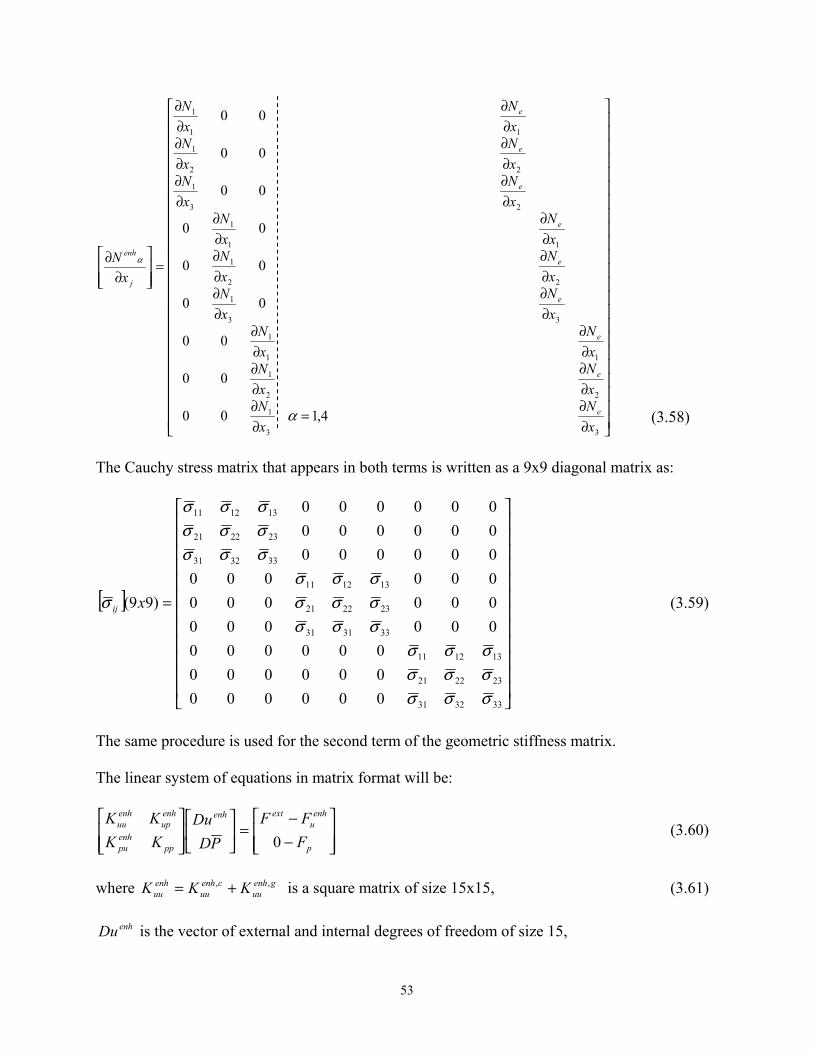
⎥⎥⎥⎥⎥⎥⎥⎥⎥⎥⎥⎥⎥⎥⎥⎥⎥⎥⎥⎥⎥⎥⎥
⎦
⎤
⎢⎢⎢⎢⎢⎢⎢⎢⎢⎢⎢⎢⎢⎢⎢⎢⎢⎢⎢⎢⎢⎢⎢
⎣
⎡
∂∂
=∂∂
∂∂
∂∂
∂∂
∂∂
∂∂
∂∂
∂∂
∂∂
∂∂
∂∂
∂∂
∂∂
∂∂
∂∂
∂∂
∂∂
=⎥⎥⎦
⎤
⎢⎢⎣
⎡∂
∂
33
1
22
1
11
1
33
1
22
1
11
1
23
1
22
1
11
1
4,100
00
00
00
00
00
00
00
00
xN
xN
xN
xN
xN
xN
xN
xN
xN
xN
xN
xN
xN
xN
xN
xN
xN
xN
xN
e
e
e
e
e
e
e
e
e
j
enh
α
α
(3.58)
The Cauchy stress matrix that appears in both terms is written as a 9x9 diagonal matrix as:
[ ]
⎥⎥⎥⎥⎥⎥⎥⎥⎥⎥⎥⎥
⎦
⎤
⎢⎢⎢⎢⎢⎢⎢⎢⎢⎢⎢⎢
⎣
⎡
=
333231
232221
131211
333131
232221
131211
333231
232221
131211
000000000000000000
000000000000000000000000000000000000
)99(
σσσσσσσσσ
σσσσσσσσσ
σσσσσσσσσ
σ xij (3.59)
The same procedure is used for the second term of the geometric stiffness matrix.
The linear system of equations in matrix format will be:
⎥⎥⎦
⎤
⎢⎢⎣
⎡−−
=⎥⎦
⎤⎢⎣
⎡
⎥⎥⎦
⎤
⎢⎢⎣
⎡
p
enhu
extenh
ppenhpu
enhup
enhuu
FFF
PDDu
KKKK
0 (3.60)
where is a square matrix of size 15x15, (3.61) genhuu
cenhuu
enhuu KKK ,, +=
enhDu is the vector of external and internal degrees of freedom of size 15,
53
enhuF is the internal force resulting from the equilibrium equation and,
hpF is the internal force resulting from the constraint equation.
5. Internal Forces
From the first term of the principle of virtual work the internal force due to the displacement
degrees of freedom can be computed as:
dVBFV
Tenhenhu σ⋅= ∫ )( (3.62)
where )( PP −+= Iσσ is the modified Cauchy stress at time t+∆t obtained from the strain
increment using the Jaumann stress rate and integrated numerically over the substep.
From the second term of the principle of virtual work,
dVPV
venhv δεε )(∫ − ,
we can compute the fictitious internal force due to the mixed u/p formulation as:
dVK
PDDPdVK
PPDDP
dVPDCKK
PD
dVPDDCKK
PDDF
VV
Vklijkl
ij
Vvklijkl
ijvp
1)(1)(
31
3
⋅−=−=
=⎟⎟⎠
⎞⎜⎜⎝
⎛+−=
=⎟⎟⎠
⎞⎜⎜⎝
⎛−+−=
∫∫
∫
∫
Nδ
δεδ
δεεδ
ε
(3.63)
where ( ) ( tttttttttttt PPDP 321321 31
31 σσσσσσ ++−++=−= ∆+∆+∆+∆+ ) (3.64)
and the Cauchy stresses at time t are stored from the previous substep.
54
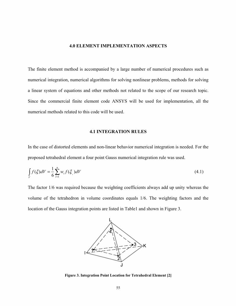
4.0 ELEMENT IMPLEMENTATION ASPECTS
The finite element method is accompanied by a large number of numerical procedures such as
numerical integration, numerical algorithms for solving nonlinear problems, methods for solving
a linear system of equations and other methods not related to the scope of our research topic.
Since the commercial finite element code ANSYS will be used for implementation, all the
numerical methods related to this code will be used.
4.1 INTEGRATION RULES
In the case of distorted elements and non-linear behavior numerical integration is needed. For the
proposed tetrahedral element a four point Gauss numerical integration rule was used.
dVfwdVfi
V
n
li )(
61)(
1
ξξ∫ ∑=
= (4.1)
The factor 1/6 was required because the weighting coefficients always add up unity whereas the
volume of the tetrahedron in volume coordinates equals 1/6. The weighting factors and the
location of the Gauss integration points are listed in Table1 and shown in Figure 3.
Figure 3. Integration Point Location for Tetrahedral Element [2]
55
Table 1. Numerical Integration for Tetrahedral Element [2]
Type Integration Point Location Weighting Factor 4 corner points
250101381966011.0249685854101966.0
432
1
====
ξξξξ
Permute ξ1, ξ2, ξ3, ξ4 for other locations
0.250000000000000
Since stiffness matrices and internal forces are all expressed as integrals over the volume of
the element we need an expression for the volume of the tetrahedral element. This is given by the
determinant of the Jacobian transformation matrix between volume and Cartesian coordinates as:
3
3
2
3
1
3
3
2
2
2
1
2
3
1
2
1
1
1
61
ξξξ
ξξξ
ξξξ
∂∂
∂∂
∂∂
∂∂
∂∂
∂∂
∂∂
∂∂
∂∂
==
xxx
xxx
xxx
JacdV (4.2)
which can be derived from:
⎥⎥⎥⎥
⎦
⎤
⎢⎢⎢⎢
⎣
⎡
⎥⎥⎥
⎦
⎤
⎢⎢⎢
⎣
⎡=
⎥⎥⎥
⎦
⎤
⎢⎢⎢
⎣
⎡
4
3
2
1
43
33
23
13
42
32
22
12
41
31
21
11
3
2
1
ξξξξ
xxxxxxxxxxxx
xxx
(4.3)
where are the Cartesian coordinates of node α. αix
This volume is a signed quantity which means that it is positive if the corner nodes are
numbered in a special way. To avoid problems with negative volumes, a special subroutine was
inserted at the beginning of the user element subroutine in which the volumes for each element
were calculated and checked for negative values.
56
If the volume was found to be negative the sign was changed and stored so it would be
accessible at each iteration. Inside the Gauss integration loop the element volume was always
multiplied with the sign saved.
4.2 NONLINEAR ITERATIVE ALGORITHM
It was shown in chapter 3 that by using an Updated Lagrangian Formulation the element
matrices and load vectors were derived. They can be arranged as a linear system of equations of
the form expressed in (3.61) or in an expanded form as:
)19(⎥⎥⎥
⎦
⎤
⎢⎢⎢
⎣
⎡ −=
⎥⎥⎥
⎦
⎤
⎢⎢⎢
⎣
⎡
⎥⎥⎥
⎦
⎤
⎢⎢⎢
⎣
⎡
(4)F(3)F
(12)FF
(4)pD(3)Du
Du(12)
(4x4)K(4x3)K(4x12)K(3x4)K(3x3)K(3x12)K(12x4)K(12x3)K(12x12)K
p
e
uext
(19)
e
(19,19)pppepu
epeeeu
upueuu
(4.4)
where the second row and second column in the element stiffness matrix are actually the last
three rows and last three columns of the enhanced stiffness matrix. In other words
matrices are just parts of the enhanced (15,15) matrix. The sizes of the partitioned matrices
and vectors are shown in the parentheses.
eepeue KKK ,,
uuK
Since the proposed interpolations for u and p are continuous in the whole domain, and the
enhanced strain parameters are introduced only internally in the element, the solution can be
performed in two steps. In the first step the internal displacements ue are eliminated at the
element level by static condensation. In the second step the reduced stiffness matrix obtained
from the first step, together with the residuals, are assembled into the global equations to be
solved using the Newton- Raphson iterative algorithm.
57
4.2.1 Static Condensation Procedure
In order to solve for the internal displacements, we first need to swap the rows and columns
corresponding to the internal parameters with the rows and columns corresponding to the
pressure variables. This is done so the final element arrays will have only the displacement and
pressure degrees of freedom. The final size of the stiffness matrix, load vector and the vector of
the external degrees of freedom has to be 12+4=16. The following steps were performed in the
static condensation procedure:
1. Introduce one row and one column of zeros in the 16th place of the enhanced stiffness
matrix which will be now (20, 20).
2. Swap the rows and columns corresponding to and eu p such that the internal parameters
will be arranged the last and the pressures in the middle. The last row and the last column
of the matrix will be all zeros and will be eliminated together with the residuals. The
system will now have the form:
⎥⎥⎥
⎦
⎤
⎢⎢⎢
⎣
⎡
−−−
=⎥⎥⎥
⎦
⎤
⎢⎢⎢
⎣
⎡
⎥⎥⎥
⎦
⎤
⎢⎢⎢
⎣
⎡
e
p
uext
eeeepeu
pepppu
ueupuu
F0F0
FF
(3)Du(4)pD
Du(12)
(3x3)K(3x4)K(3x12)K(4x3)K(4x4)K(4x12)K
(12x3)K(12x4)K(12x12)K (4.5)
3. Partition the matrices as:
(4.6) ⎥⎦
⎤⎢⎣
⎡−
=⎥⎦
⎤⎢⎣
⎡⎥⎦
⎤⎢⎣
⎡
e
1
e
final
ee21
1211
FF
DuDu
(3x3)K(3x16)K(16x3)K(16x16)K
⎥⎦
⎤⎢⎣
⎡=
(4x4)K(4x12)K(12x4)K(12x12)K
Kpppu
upuu11 (4.7)
⎥⎦
⎤⎢⎣
⎡=
(4x3)K(12x3)K
Kpe
ue12 (4.8)
58
[ ](3x4)K(3x12)KK epeu21 = (4.9)
⎥⎦
⎤⎢⎣
⎡=
pDDu
Dufinal (4.10)
⎥⎥⎦
⎤
⎢⎢⎣
⎡−−
=p
uext
1 FFF
F (4.11)
4. Store and retrieve them at the beginning of the next iteration
to calculate the iterative value of the internal displacement degrees of freedom.
(4.12)
eF*)(K,K*)(K 1ee21
1ee
−−
[ ] )DuK(FKDu iter21e
1eee
iter ⋅−−= −
The increment of the internal displacements is obtained as an accumulation of each
iteration value and is stored if the iteration converged.
∑= itere
substepe DuDu (4.13)
5. Substitute in the first equation to get the final stiffness matrix of size (16,16):
(4.14) 1finalfinal211
ee1211finalfinal FDu)K*K*K(KuK =⋅−=⋅ −D
6. Calculate reduced internal force as: (4.15) eF*)(KFF 1ee11final
−−=
7. From here the assembly of final element matrix and residual into global equations
proceeds to find out the incremental values of nodal displacements and pressures.
59
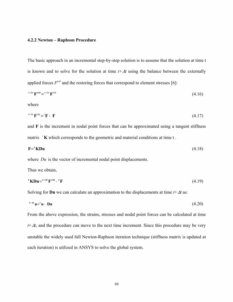
4.2.2 Newton – Raphson Procedure
The basic approach in an incremental step-by-step solution is to assume that the solution at time t
is known and to solve for the solution at time t+∆t using the balance between the externally
applied forces Fext and the restoring forces that correspond to element stresses [6]:
intFFext tttt ∆+∆+ = (4.16)
where
FFF +=∆+ ttt int (4.17)
and F is the increment in nodal point forces that can be approximated using a tangent stiffness
matrix Kt which corresponds to the geometric and material conditions at time t .
KDuF t= (4.18)
where is the vector of incremental nodal point displacements. Du
Thus we obtain,
FFKDu text∆ttt −= + (4.19)
Solving for Du we can calculate an approximation to the displacements at time t+∆t as:
Duuu t∆tt +=+ (4.20)
From the above expression, the strains, stresses and nodal point forces can be calculated at time
t+∆t, and the procedure can move to the next time increment. Since this procedure may be very
unstable the widely used full Newton-Raphson iteration technique (stiffness matrix is updated at
each iteration) is utilized in ANSYS to solve the global system.
60

The equations used in the Newton-Raphson iteration are:
(i)1)(i∆tt(i)∆tt
1)(i∆ttext∆tt(i)1)(i∆tt
DuuuFFDuK
+=−=
−++
−++−+
(4.21)
with the initial conditions:
(4.22) FFKK
uu
t(0)∆tt
t(0)∆tt
t(0)∆tt
===
+
+
+
The general algorithm for a substep at iteration (i) is illustrated in Figure 4 and can be described
as follows[2]:
1. Assume u0 which is usually the converged solution from previous time step and for the
first iteration of the first substep is just zero.
2. Compute the updated element stiffness matrix, strains and stresses, which in inelastic
analysis are obtained by an integration process, and using (3.63) compute the restoring
load.
3. Check equilibrium and if the restoring load is not equal (or at least to within some
tolerance) to the applied force then compute Du(i) using first equation of (4.20).
4. Update the displacement to obtain the next approximation using second equation of
(4.20).
5. Repeat steps 2 to 4 until convergence is achieved.
61
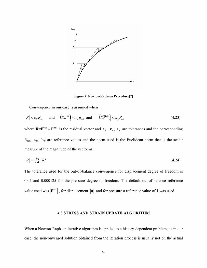
Figure 4. Newton-Raphson Procedure[2]
Convergence in our case is assumed when
refR RεR < and ( ) refu(i) uεDu < and ( ) refp
(i) PεPD < (4.23)
where R=Fext – Fint is the residual vector and , , are tolerances and the corresponding
R
Rε uε pε
ref, uref, Pref are reference values and the norm used is the Euclidean norm that is the scalar
measure of the magnitude of the vector as:
∑= 2iRR (4.24)
The tolerance used for the out-of-balance convergence for displacement degree of freedom is
0.05 and 0.000125 for the pressure degree of freedom. The default out-of-balance reference
value used was extF , for displacement u and for pressure a reference value of 1 was used.
4.3 STRESS AND STRAIN UPDATE ALGORITHM
When a Newton-Raphson iterative algorithm is applied to a history-dependent problem, as in our
case, the nonconverged solution obtained from the iteration process is usually not on the actual
62
path and thus, the strain and stress which are history-dependent variables have to be integrated
over the increment each iteration [1]. They cannot be computed as the sum of the integrations
performed in each iteration. We assume though that the primary variables are varying linearly
over the increment.
In our formulation the strain is defined as the integral of the strain rate. This integration has to
take into account the fact that the principal axes of strain rotate during the deformation.
Therefore the strain at the beginning of the increment must be rotated with the amount of rigid
body rotation that occurs during that increment. This is done using the Hughes-Winget [27]
algorithm. According to Hughes-Winget, any tensor associated with a rate constitutive equation
is integrated as:
)(Dεa∆∆Ra∆Ra Tt∆tt
(+⋅⋅=+ (4.25)
where a is the tensor, a∆( is the increment associated with the material’s constitutive behavior
which depends on the strain increment, , defined by the central difference formula as: Dε
)(2/ttx
DusymD∆+∂
∂=ε (4.26)
where
)(21
2/ ttttt xxx ∆+∆+ += (4.27)
and is the rotation matrix computed from the polar decomposition of the deformation
gradient at the midpoint configuration:
∆R
2/12/12/1 URF ∆⋅∆=∆ (4.28)
63
The displacement increment at midpoint configuration,
∆t/2t
∆tt
∆tt∆t/2t xx
xDu
xDu
+
+
++ ∂∂
⋅∂∂=
∂∂ (4.29)
is computed from the increment of deformation gradient evaluated at the midpoint configuration:
1
1
−
+
−
+
+−
+
+
+
+⎟⎟⎠
⎞⎜⎜⎝
⎛∂∂−=
⎟⎟⎟⎟
⎠
⎞
⎜⎜⎜⎜
⎝
⎛
∂
−∂=
∂∂
=∂∂
)xDu(
21I
x
Du)21(x
)xx
(xx
∆tt∆tt
∆tt1
∆tt
∆t/2t
∆t/2t
∆tt (4.30)
and DuBxDu
∆ttenh
∆tt
⋅=∂∂
+
+
(4.31)
yielding
1
∆tt∆tt∆t/2t
)xDu
21(I*
xDu
xDu −
+++ ∂∂−
∂∂=
∂∂ (4.32)
If and the strains, , are known then we proceed to calculate the stresses
which in inelastic analysis are obtained by the above described integration process as
in (4.25).
)1( −∆+ it Ut )1( −∆+ it εt
)1( −∆+ it σt
64
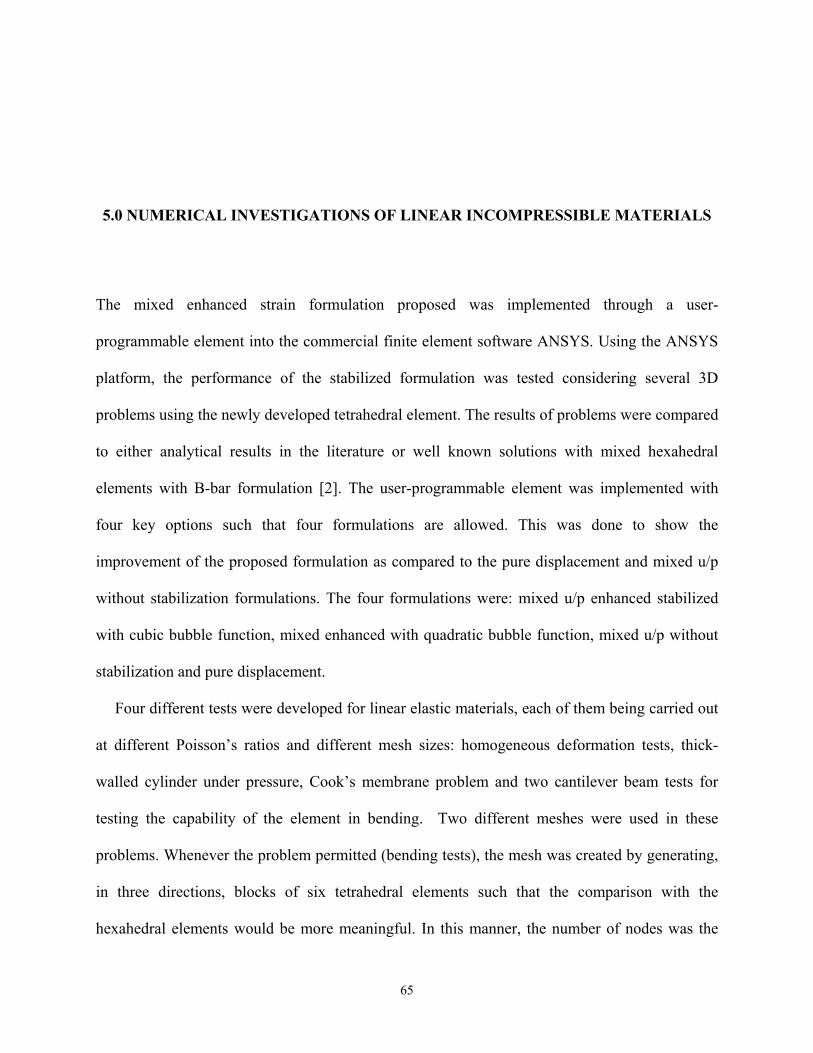
5.0 NUMERICAL INVESTIGATIONS OF LINEAR INCOMPRESSIBLE MATERIALS
The mixed enhanced strain formulation proposed was implemented through a user-
programmable element into the commercial finite element software ANSYS. Using the ANSYS
platform, the performance of the stabilized formulation was tested considering several 3D
problems using the newly developed tetrahedral element. The results of problems were compared
to either analytical results in the literature or well known solutions with mixed hexahedral
elements with B-bar formulation [2]. The user-programmable element was implemented with
four key options such that four formulations are allowed. This was done to show the
improvement of the proposed formulation as compared to the pure displacement and mixed u/p
without stabilization formulations. The four formulations were: mixed u/p enhanced stabilized
with cubic bubble function, mixed enhanced with quadratic bubble function, mixed u/p without
stabilization and pure displacement.
Four different tests were developed for linear elastic materials, each of them being carried out
at different Poisson’s ratios and different mesh sizes: homogeneous deformation tests, thick-
walled cylinder under pressure, Cook’s membrane problem and two cantilever beam tests for
testing the capability of the element in bending. Two different meshes were used in these
problems. Whenever the problem permitted (bending tests), the mesh was created by generating,
in three directions, blocks of six tetrahedral elements such that the comparison with the
hexahedral elements would be more meaningful. In this manner, the number of nodes was the
65
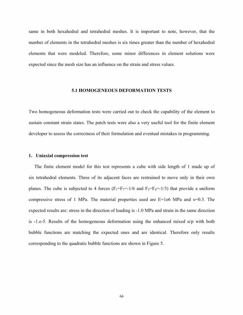
same in both hexahedral and tetrahedral meshes. It is important to note, however, that the
number of elements in the tetrahedral meshes is six times greater than the number of hexahedral
elements that were modeled. Therefore, some minor differences in element solutions were
expected since the mesh size has an influence on the strain and stress values.
5.1 HOMOGENEOUS DEFORMATION TESTS
Two homogeneous deformation tests were carried out to check the capability of the element to
sustain constant strain states. The patch tests were also a very useful tool for the finite element
developer to assess the correctness of their formulation and eventual mistakes in programming.
1. Uniaxial compression test
The finite element model for this test represents a cube with side length of 1 made up of
six tetrahedral elements. Three of its adjacent faces are restrained to move only in their own
planes. The cube is subjected to 4 forces (F1=F7=-1/6 and F5=F4=-1/3) that provide a uniform
compressive stress of 1 MPa. The material properties used are E=1e6 MPa and υ=0.3. The
expected results are: stress in the direction of loading is -1.0 MPa and strain in the same direction
is -1.e-5. Results of the homogeneous deformation using the enhanced mixed u/p with both
bubble functions are matching the expected ones and are identical. Therefore only results
corresponding to the quadratic bubble functions are shown in Figure 5.
66
(a) Stress in loading direction (b) Strain in loading direction
Figure 5. Stress and strain in the direction of loading for the uniaxial compression test
2. Homogeneous deformation of a unit cube formed of 25-tetrahedra under linear applied
displacement field
The finite element model consists of a 1x1x1 block meshed with 25 tetrahedral elements and
subjected to a linearly varying displacement field applied to all nodes as given by the following:
z*1.5 y *0.75 x *1.5 0.5z z*0.75 y *1.0 x *2.5 0.75
*5.0*5.1*0.20.1
+++=+++=+++=
vzyxu
The material properties are E=1.e6MPa and the finite element model is presented in Figure 6.
Figure 6. Finite element model of unit cube formed by 25-tetrahedra
67
The computed strains and stresses for this deformation field should be:
800000.0 600000.0, 1600000.0,
, 3000000.0 2600000.0, 3400000.0, 2.0 1.5, 4.0,
, 1.5 1.0, 2.0,
zxyzxy
zzyyxx
zxyzxy
zzyyxx
===
===
===
===
σσσσσσ
εεεεεε
The mixed enhanced tetrahedral element passed this patch test since the results obtained are
exactly as those expected. A part of the output files with strains and stresses for a few selected
elements together with expected strains and stresses is presented in Appendix B.
5.2 EXPANSION OF A THICK-WALL CYLINDER UNDER PRESSURE
This test was proposed by R. Taylor in [47] to assess the behavior of a similar strain enhanced
tetrahedral element in nearly incompressible materials.
Description of the test
An infinitely long thick walled cylinder with inner radius of 3 units and outer radius of 9 units
is subjected to an internal pressure of 1 unit. Due to the axisymmetric nature of the problem, the
finite element model can be represented by a wedge of a 5 degree angle sector and a unit
thickness. The material properties considered are linear elastic with E = 1.e6 and Poisson’s ratios
were varied from 0, 0.25, 0.3, 0.49, 0.499 and 0.4999 to evaluate the robustness of the
formulation. The mesh is unstructured and the number of divisions per radial direction was
varied from N=10, 20 to 30 elements. Results of each formulation are compared with the
theoretical results and errors are reported in Tables 2, 3 and 4.
68
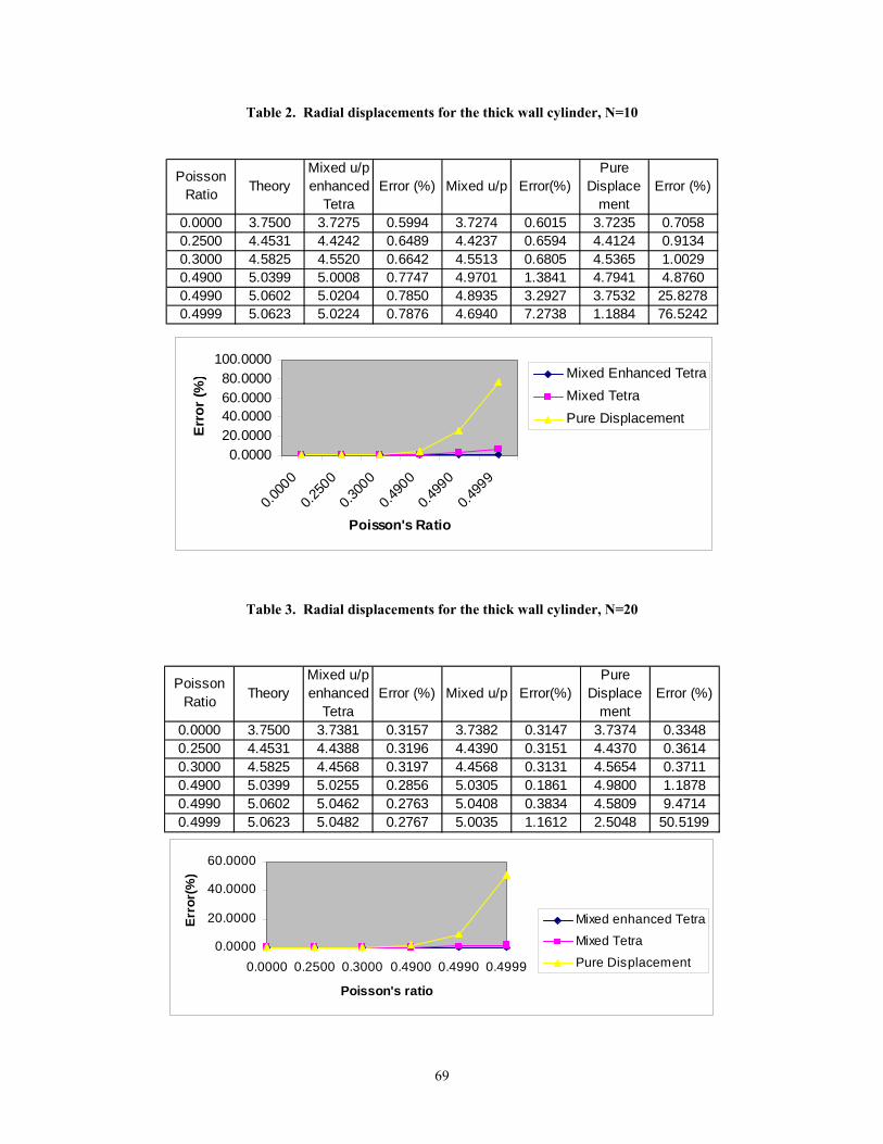
Table 2. Radial displacements for the thick wall cylinder, N=10
Poisson Ratio Theory
Mixed u/p enhanced
Tetra Error (%) Mixed u/p Error(%)
Pure Displace
mentError (%)
0.0000 3.7500 3.7275 0.5994 3.7274 0.6015 3.7235 0.70580.2500 4.4531 4.4242 0.6489 4.4237 0.6594 4.4124 0.91340.3000 4.5825 4.5520 0.6642 4.5513 0.6805 4.5365 1.00290.4900 5.0399 5.0008 0.7747 4.9701 1.3841 4.7941 4.87600.4990 5.0602 5.0204 0.7850 4.8935 3.2927 3.7532 25.82780.4999 5.0623 5.0224 0.7876 4.6940 7.2738 1.1884 76.5242
0.000020.000040.000060.000080.0000
100.0000
0.000
0
0.250
0
0.300
0
0.490
0
0.499
0
0.499
9
Poisson's Ratio
Erro
r (%
) Mixed Enhanced TetraMixed TetraPure Displacement
Table 3. Radial displacements for the thick wall cylinder, N=20
Poisson Ratio Theory
Mixed u/p enhanced
Tetra Error (%) Mixed u/p Error(%)
Pure Displace
mentError (%)
0.0000 3.7500 3.7381 0.3157 3.7382 0.3147 3.7374 0.33480.2500 4.4531 4.4388 0.3196 4.4390 0.3151 4.4370 0.36140.3000 4.5825 4.4568 0.3197 4.4568 0.3131 4.5654 0.37110.4900 5.0399 5.0255 0.2856 5.0305 0.1861 4.9800 1.18780.4990 5.0602 5.0462 0.2763 5.0408 0.3834 4.5809 9.47140.4999 5.0623 5.0482 0.2767 5.0035 1.1612 2.5048 50.5199
0.0000
20.0000
40.0000
60.0000
0.0000 0.2500 0.3000 0.4900 0.4990 0.4999
Poisson's ratio
Erro
r(%
)
Mixed enhanced Tetra
Mixed Tetra
Pure Displacement
69
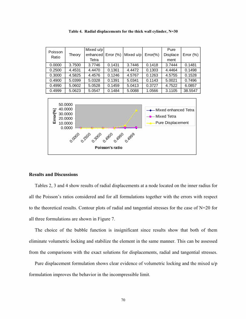
Table 4. Radial displacements for the thick wall cylinder, N=30
Poisson Ratio Theory
Mixed u/p enhanced
Tetra Error (%) Mixed u/p Error(%)
Pure Displace
mentError (%)
0.0000 3.7500 3.7746 0.1431 3.7446 0.1418 3.7444 0.14810.2500 4.4531 4.4470 0.1361 4.4472 0.1303 4.4464 0.14980.3000 4.5825 4.4576 0.1246 4.5767 0.1263 4.5755 0.15280.4900 5.0399 5.0328 0.1391 5.0341 0.1143 5.0021 0.74960.4990 5.0602 5.0528 0.1459 5.0413 0.3727 4.7522 6.08570.4999 5.0623 5.0547 0.1484 5.0088 1.0566 3.1105 38.5547
0.000010.000020.000030.000040.000050.0000
0.000
0
0.250
0
0.300
0
0.490
0
0.499
0
0.499
9
Poisson's ratio
Err
or(%
) Mixed enhanced TetraMixed TetraPure Displacement
Results and Discussions
Tables 2, 3 and 4 show results of radial displacements at a node located on the inner radius for
all the Poisson’s ratios considered and for all formulations together with the errors with respect
to the theoretical results. Contour plots of radial and tangential stresses for the case of N=20 for
all three formulations are shown in Figure 7.
The choice of the bubble function is insignificant since results show that both of them
eliminate volumetric locking and stabilize the element in the same manner. This can be assessed
from the comparisons with the exact solutions for displacements, radial and tangential stresses.
Pure displacement formulation shows clear evidence of volumetric locking and the mixed u/p
formulation improves the behavior in the incompressible limit.
70
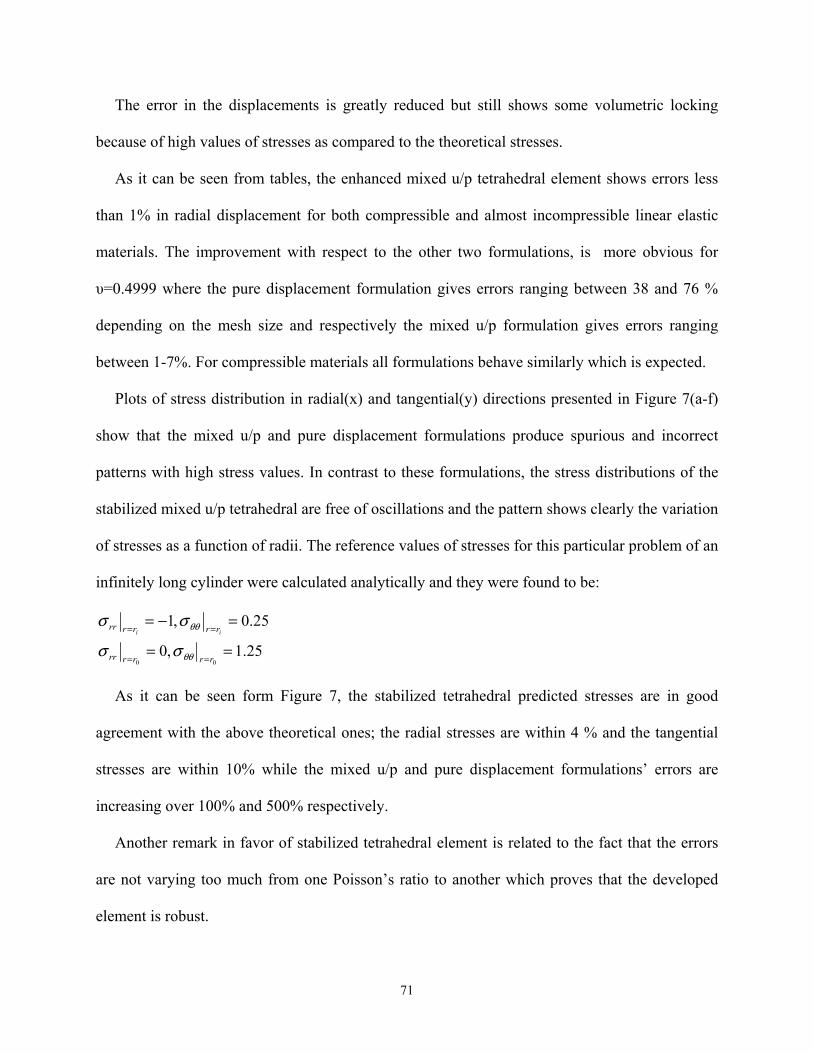
The error in the displacements is greatly reduced but still shows some volumetric locking
because of high values of stresses as compared to the theoretical stresses.
As it can be seen from tables, the enhanced mixed u/p tetrahedral element shows errors less
than 1% in radial displacement for both compressible and almost incompressible linear elastic
materials. The improvement with respect to the other two formulations, is more obvious for
υ=0.4999 where the pure displacement formulation gives errors ranging between 38 and 76 %
depending on the mesh size and respectively the mixed u/p formulation gives errors ranging
between 1-7%. For compressible materials all formulations behave similarly which is expected.
Plots of stress distribution in radial(x) and tangential(y) directions presented in Figure 7(a-f)
show that the mixed u/p and pure displacement formulations produce spurious and incorrect
patterns with high stress values. In contrast to these formulations, the stress distributions of the
stabilized mixed u/p tetrahedral are free of oscillations and the pattern shows clearly the variation
of stresses as a function of radii. The reference values of stresses for this particular problem of an
infinitely long cylinder were calculated analytically and they were found to be:
25.1,0
25.0,1
00==
=−=
==
==
rrrrrr
rrrrrrii
θθ
θθ
σσ
σσ
As it can be seen form Figure 7, the stabilized tetrahedral predicted stresses are in good
agreement with the above theoretical ones; the radial stresses are within 4 % and the tangential
stresses are within 10% while the mixed u/p and pure displacement formulations’ errors are
increasing over 100% and 500% respectively.
Another remark in favor of stabilized tetrahedral element is related to the fact that the errors
are not varying too much from one Poisson’s ratio to another which proves that the developed
element is robust.
71
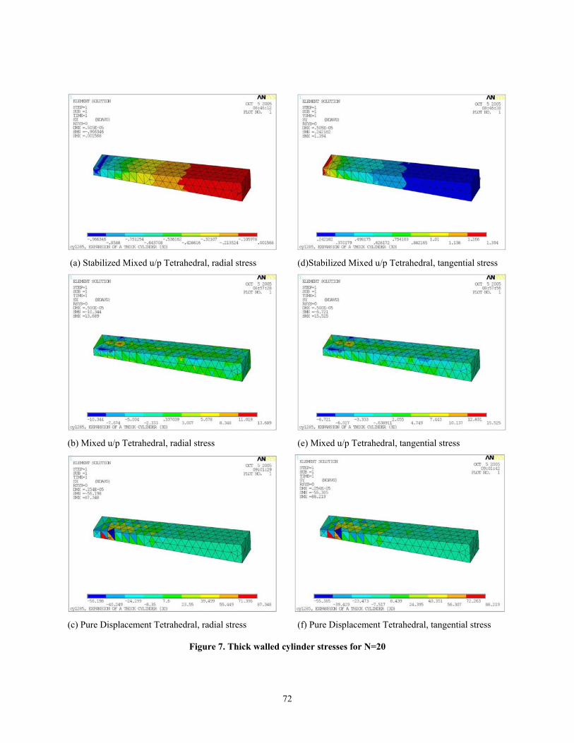
(d)Stabilized Mixed u/p Tetrahedral, tangential stress
(b) Mixed u/p Tetrahedral, radial stress (e) Mixed u/p Tetrahedral, tangential stress
(c) Pure Displacement Tetrahedral, radial stress (f) Pure Displacement Tetrahedral, tangential stress
Figure 7. Thick walled cylinder stresses for N=20
(a) Stabilized Mixed u/p Tetrahedral, radial stress
72
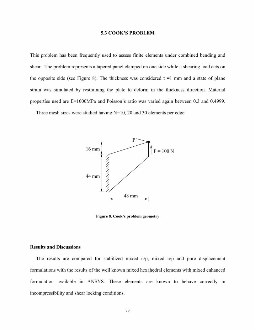
5.3 COOK’S PROBLEM
This problem has been frequently used to assess finite elements under combined bending and
shear. The problem represents a tapered panel clamped on one side while a shearing load acts on
the opposite side (see Figure 8). The thickness was considered t =1 mm and a state of plane
strain was simulated by restraining the plate to deform in the thickness direction. Material
properties used are E=1000MPa and Poisson’s ratio was varied again between 0.3 and 0.4999.
Three mesh sizes were studied having N=10, 20 and 30 elements per edge.
Figure 8. Cook’s problem geometry
Results and Discussions
The results are compared for stabilized mixed u/p, mixed u/p and pure displacement
formulations with the results of the well known mixed hexahedral elements with mixed enhanced
formulation available in ANSYS. These elements are known to behave correctly in
incompressibility and shear locking conditions.
48 mm
F = 100 N
P
16 mm
44 mm
73
Tables 5 and 6 represent the vertical displacement of the top corner node P, the axial stresses
for all formulations and the errors with respect to the hexahedral elements. Figures 9, 10 and 11
show contour plots of the normal stresses in x and y direction and shear stresses for all
formulations for the mesh size N=20 and Poisson ratio υ=0.4999.
The pure displacement formulation exhibits severe locking behavior as the error in the
displacement of point P reaches 42 % and the stresses are highly overestimated. The mixed u/p
elements show improved accuracy in displac ts (error is just 1.7%) but the stresses show
spurious distribution and are overestimated.
The stabilized tetrahedral elements approach very closely the hexahedral element solution in
both displacements and stress distribution. They yield accurate results even on coarse meshes
with just 0.16% error in displacements and within 5% error in stresses. Also they yield a smooth
stress distribution for all the situations considered. The difference that can be noted in axial
compressive stresses when compared to th xahedral elements is due to the unstructured
e ents w he
left top corner.
As for the shear stresses, the mixed u/p and stabilized mixed u/p yield similar results and
istribution patterns which are very close to the hexahedral results. This is explained by the fact
that the shear component of the stresses does not contain the volumetric part and therefore is not
affected by the increasing pressures developed in cases of volumetric locking.
emen
e he
mesh that was used for the tetrahedral el m hich produces highly distorted elements at t
d
74
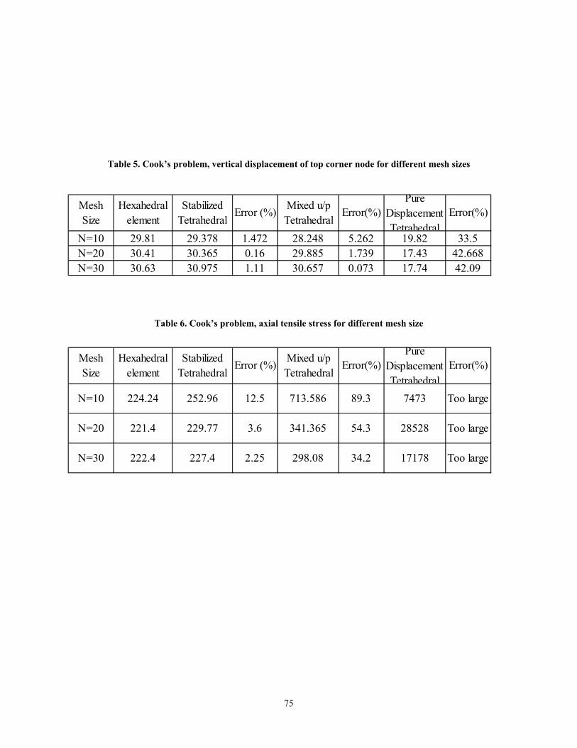
Table 5. Cook’s al displacement of top corner node for different mesh sizes
problem, vertic
N=10 29.81 29.378 1.472 28.248 5.262 19.82 33.5N=20 30.41 30.365 9 17.43 42.668N=30 30.63 30.975 1.11 30.657 0.073 17.74 42.09
Stabilized Tetrahedral
/p al
Error(%)Mesh Size
Hexahedral element
Mixed uTetrahedr
0.16 29.885 1.73
Pure Displacement Tetrahedral
Error (%) Error(%)
Cook’s problem, axial tensile stress for different mesh size
Table 6.
N=10 224.24 252.96 12.5 713.586 89.3 7473 Too large
N=20 221.4 229.77 3.6
Stabilized Tetrahedral
Mixed u/p Tetrahedral
Mesh Size
Hexahedral element
341.365 54.3 28528 Too large
N
Error(%)Pure
Displacement Tetrahedral
=30 222.4 227.4 2.25 298.08 34.2 17178 Too large
Error (%) Error(%)
75
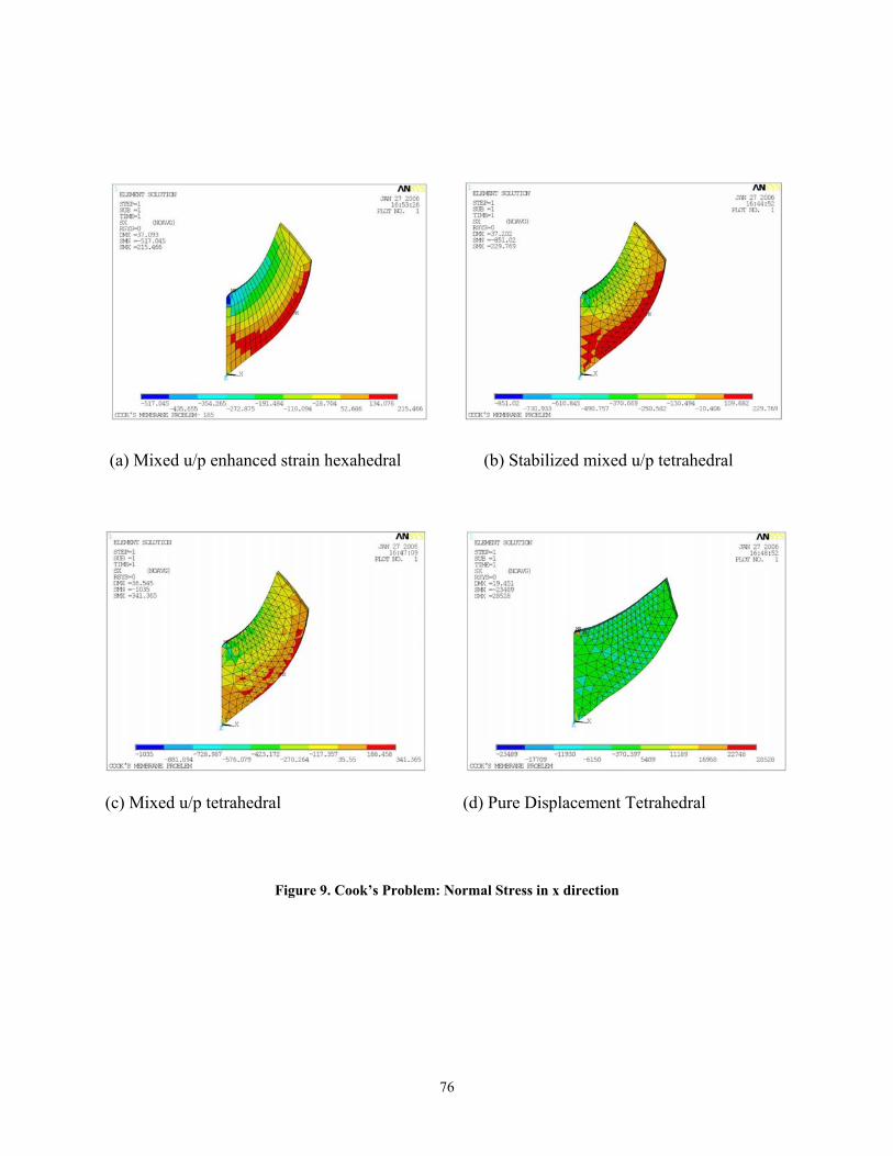
(a) Mixed u/p enhanced strain hexahedral (b) Stabilized mixed u/p tetrahedral
(c) Mixed u/p tetrahedral (d) Pure Displacement Tetrahedral
Figure 9. Cook’s Problem: Normal Stress in x direction
76
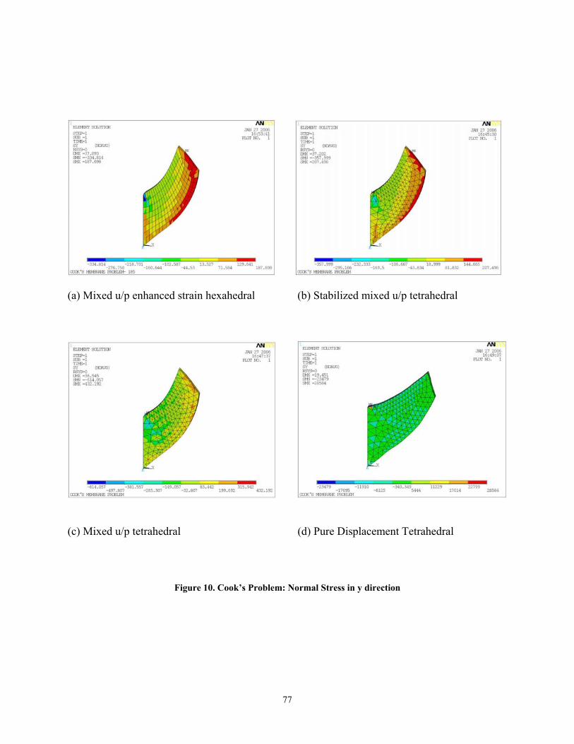
77
(a) Mixed u/p enhanced strain hexahedral (b) Stabilized mixed u/p tetrahedral
(c) Mixed u/p tetrahedral (d) Pure Displacement Tetrahedral
Figure 10. Cook’s Problem: al Stress in y direction
Norm
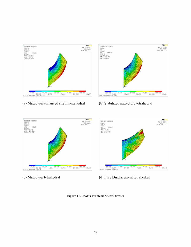
(b) Stabilized mixed u/p tetrahedral
(d) Pure Displacement tetrahedral
Problem: Shear Stresses
(a) Mixed u/p enhanced strain hexahedral
(c) Mixed u/p tetrahedral
Figure 11. Cook’s
78
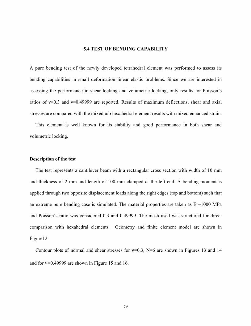
5.4 TEST OF BENDING CAPABILITY
pure bending test of the newly developed tetrahedral element was performed to assess its
ending capabilities in small deformation linear elastic problems. Since we are interested in
ssessing the performance in shear locking and volumetric locking, only results for Poisson’s
stresses are compared with the mixed u/p hexahedr
This element is well known for its stabil
volumetric locking.
Description of the test
The test represents a cantilever beam with on with width of 10 mm
hickness of 2 mm and length of 100 mm clamped at the left end. A bending moment is
pplied through two opposite displacement loads along the right edges (top and bottom) such that
an extreme pure bending case is simulated. The material properties are taken as E =1000 MPa
and Poisson’s ratio was considered 0.3 and 0.49999. The mesh used was structured for direct
comparison with hexahedral elements. Geometry and finite element model are shown in
Figure12.
Contour plots of normal and shear stresses for ν=0.3, N=6 are shown in Figures 13 and 14
and for ν=0.49999 are shown in Figure 15 and 16.
A
b
a
ratios of ν=0.3 and ν=0.49999 are reported. Results of maximum deflections, shear and axial
al element results with mixed enhanced strain.
ity and good performance in both shear and
a rectangular cross secti
and t
a
79
Figure 12. Finite element model of the pure bending test
Results and Discussions
From the two sets of plots it can be deduced that the tetrahedral element’s performance in
ending.
ven though the displacements are within errors of 1 % and the normal stresses are acceptable,
the shear stresses have nced strain hexahedral
lements. The shear stress distribution also shows evidence of locking. When both shear and
compressibility constraints exist, the stabilized tetrahedral brings some improvement as
ompared to the mixed u/p and pure displacement formulation that is completely locked as it can
e seen from Figure 15. This remark helps us conclude that the stabilized tetrahedron is
erforming poorer than the mixed u/p enhanced strain hexahedral element in pure bending
s. It is though necessary to note that in bending dominant problems, as it was seen for
Cook’s problem, this limitation disappears and the performance is significantly improved.
100
10
2
shear locking is not as good as it is in volumetric locking for this extreme case of pure b
E
larger values than those obtained using mixed enha
e
in
c
b
p
problem
80
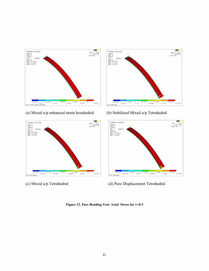
(a) Mixed u/p enhanced strain hexahedral
(b) Stabilized Mixed u/p Tetrahedral
(c) Mixed u/p Tetrahedral (d) Pure Displacement Tetrahedral
Figure 13. Pure Bending Test: Axial Stress for ν=0.3
81
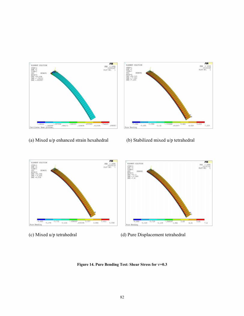
(b) Stabilized mixed u/p tetrahedral
(c) Mixed u/p tetrahedral (d) Pure Displacement tetrahedral
Figure 14. Pure Bending Test: Shear Stress for ν=0.3
(a) Mixed u/p enhanced strain hexahedral
82
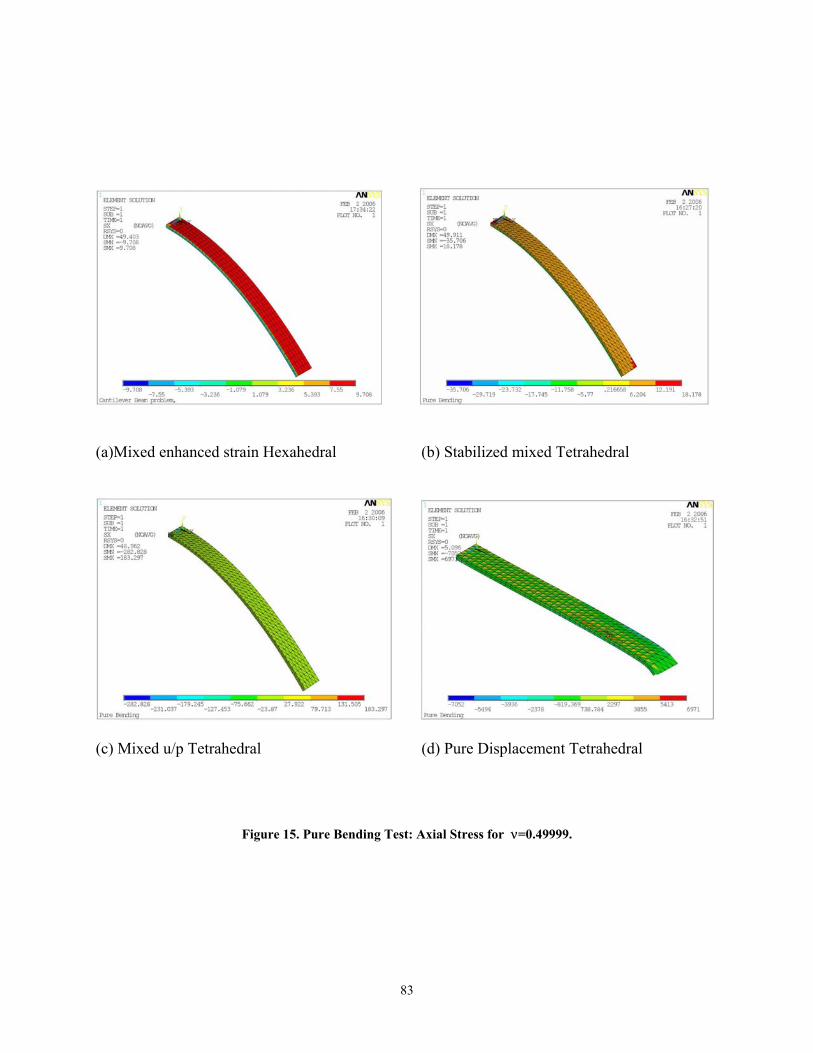
(b) Stabilized mixed Tetrahedral
(c) Mixed u/p Tetrahedral (d) Pure Displacement Tetrahedral
Figure 15. Pure Bending Test: Axial Stress for ν=0.49999.
(a)Mixed enhanced strain Hexahedral
83
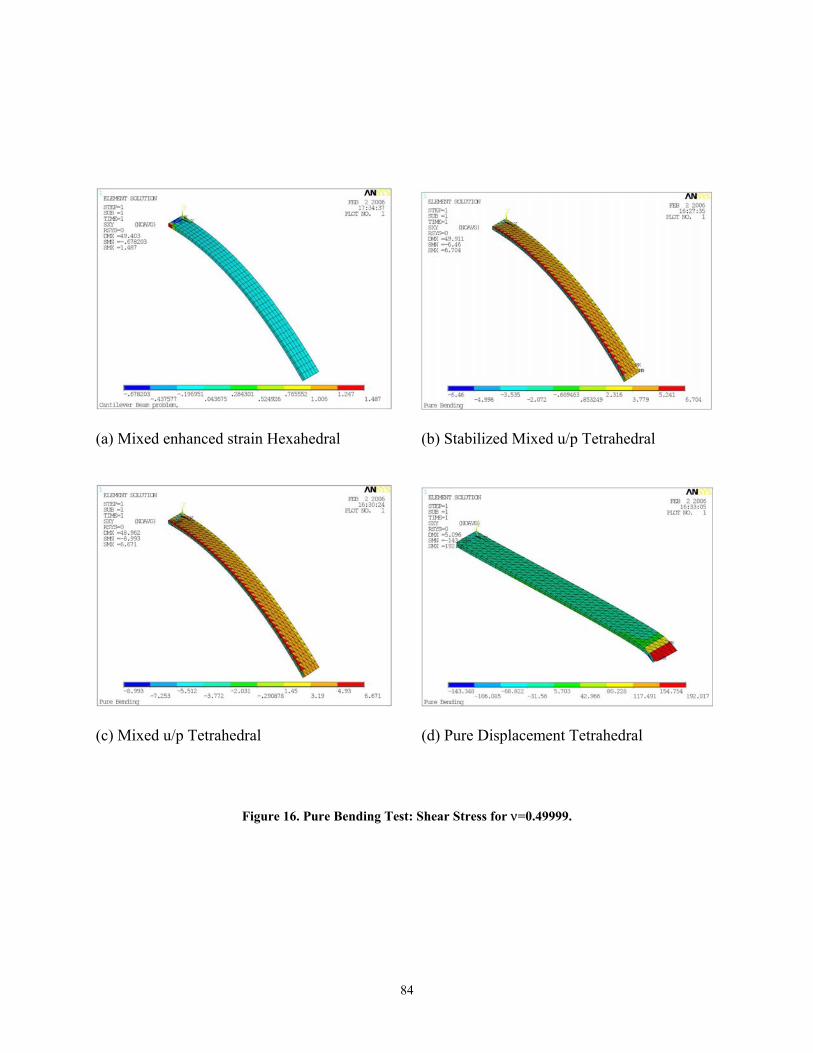
) Mixed enhanced strain Hexahedral (b) Stabilized Mixed u/p Tetrahedral
Figure 16. Pure Bending Test: Shear Stress for ν=0.49999.
(a
(c) Mixed u/p Tetrahedral (d) Pure Displacement Tetrahedral
84
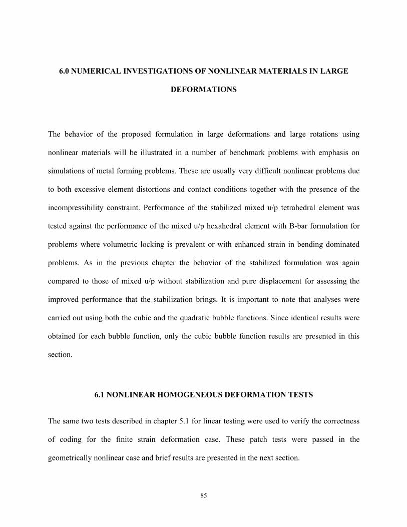
6.0 NUMERICAL INVESTIGATIONS OF NONLINEAR MATERIALS IN LARGE
DEFORMATIONS
The behavior of the proposed formulation in large deformations and large rotations using
nonlinear materials will be illustrated in a number of benchmark problems with emphasis on
simulations of metal forming problems. These are usually very difficult nonlinear problems due
to both excessive element distortions and contact conditions together with the presence of the
incompressibility constraint. Performance of the stabilized mixed u/p tetrahedral element was
problems where volumetric locking is prevalent or with enhanced strain in bending dominated
problems. As in the previous chapter the behavior of the stabilized formulation was again
compared to those of mixed u/p without stabilization and pure displacement for assessing the
improved performance that the stabilization brings. It is important to note that analyses were
carried out using both the cubic and the quadratic bubble functions. Since identical results were
for each bubble function, only the cu le function results are presented in this
6.1 NONLI S
he same two tests described in chapter 5.1 for linear testing were used to verify the correctness
f coding for the finite strain deformation case. These patch tests were passed in the
eometrically nonlinear case and brief results are presented in the next section.
tested against the performance of the mixed u/p hexahedral element with B-bar formulation for
obtained bic bubb
section.
NEAR HOMOGENEOUS DEFORMATION TEST
T
o
g
85
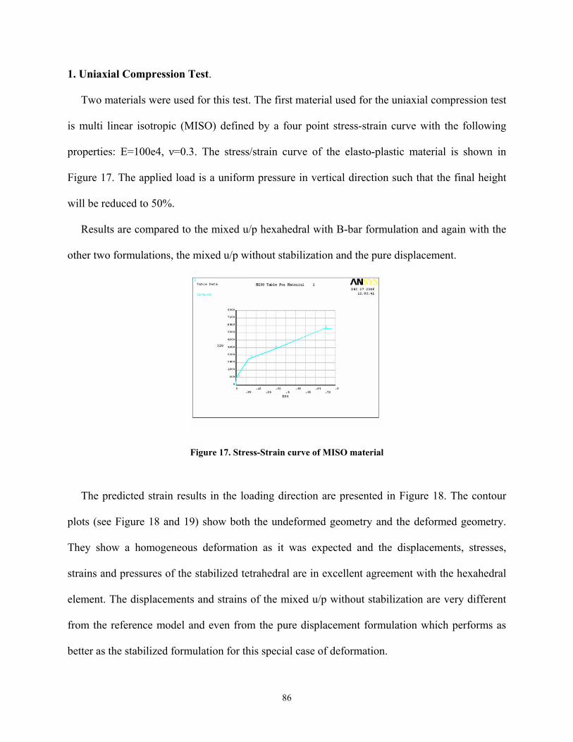
1. Uniaxial Compression Test.
Two materials were used for this test. The first material used for the uniaxial compression test
multi linear isotropic (MISO) defined by a four point stress-strain curve with the following
properties: E=100e4, ν=0.3. The stress/strain curve of the elasto-plastic material is shown in
Figure 17. The applied load is a uniform pressure in vertical direction such that the final height
will be reduced to 50%.
Results are compared to the mixed u/p hexahedral with B-bar formulation and again with the
other two formulations, the mixed u/p without stabilization and the pure displacement.
is
Figure 17. Stress-Strain curve of MISO material
The predicted strain results in the loading direction are presented in Figure 18. The contour
plots (see Figure 18 and 19) show both the und med geometry and the deformed geometry.
ts, stresses,
rains and pressures of the stabilized tetrahedral are in excellent agreement with the hexahedral
lement. The displacements and strains of the mixed u/p without stabilization are very different
from the reference mode s as
etter as the stabilized formulation for this special case of deformation.
efor
They show a homogeneous deformation as it was expected and the displacemen
st
e
l and even from the pure displacement formulation which perform
b
86
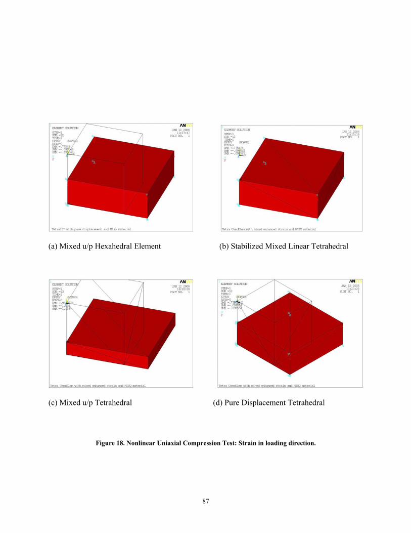
) Mixed u/p Hexahedral Element (b) Stabilized Mixed Linear Tetrahedral
(c) Mixed u/p Tetrahedral (d) Pure Displacement Tetrahedral
Figure 18. Nonlinear Uniaxial Compression Test: Strain in loading direction.
(a
87
) Mixed u/p hexahedral (b) Stabilized Mixed Tetrahedral
Figure 19. Nonlinear Uniaxial Compression Test: Hydrostatic Pressure.
The second material is modeled by a rate dependent visco-plasticity model in which the yield
strength is introduced by an overstress power law (PERZYNA model) and the static yield
strength is defined by using a bilinear isotropic model. The parameters introduced in the model
are: E=2.0e5, ν=0.3, σ0 = 9000, m (strain rate hardening parameter) = 0.2,
(Viscosity parameter)=0.4 according to the m
(a
γ odel ⎟⎟⎟
⎠
⎞⎜⎜⎜⎝
⎛⎟⎞⎜⎛+⋅=
mpleqv
y
εσσ
&10
The same boundary conditions as before are maintained and a uniform pressure in the vertical
direction is applied in three load steps as follows:
1. Apply a stress equal to the yield stress (9000).
2. Apply a stress equal to 10800.
3. Keep a constant stress at 10800.
⎟⎠⎜⎝ γ
88
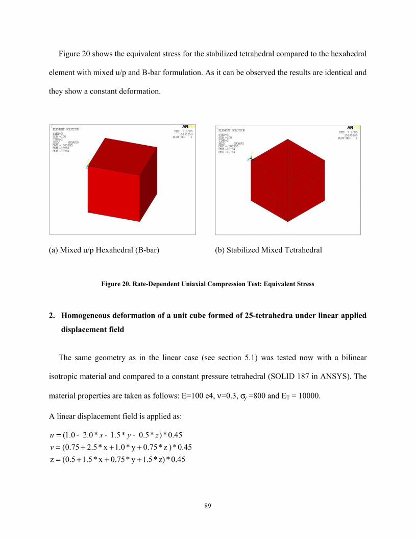
Figure 20 shows the equivalent stress for the stabilized tetrahedral compared to the hexahedral
element with mixed u/p and B-bar formulation. As it can be observed the results are identical and
they show a constant deformation.
(a) Mixed u/p Hexahedral (B-bar) (b) Stabilized Mixed Tetrahedral
Figure 20. Rate-Dependent Uniaxial Compression Test: Equivalent Stress
. Homogeneous deformation of a unit cube formed of 25-tetrahedra under linear applied
displacement field
The same geometry as in the linear case (see section 5.1) was tested now with a bilinear
otropic material and compared to a constant pressure tetrahedral (SOLID 187 in ANSYS). The
aterial properties are taken as follows: E=100 e4, ν=0.3, σy =800 and ET = 10000.
l
0*)*5.0*5.1*0.20.1(
+++=+++=
2
is
m
A inear displacement field is applied as:
45.
0.45*z)*1.5 y *0.75 x *1.5 0.5(z 0.45*) z*0.75 y *1.0 x *2.5 0.75(
+++=v
zyxu
89
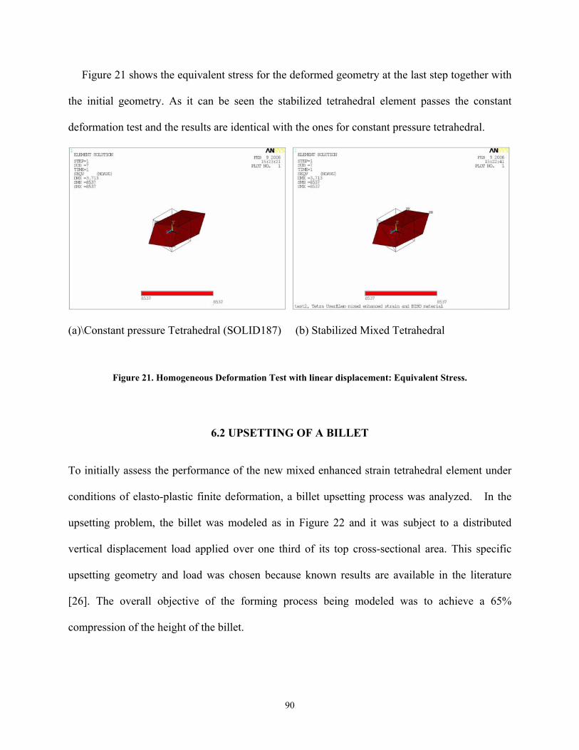
Figure 21 shows the equivalent stress for the deformed geometry at the last step together with
the initial geometry. As it can be seen the stabilized tetrahedral element passes the constant
deformation test and the results are identical with the ones for constant pressure tetrahedral.
(a)\Constant pressure Tetrahedral (SOLID187) (b) Stabilized Mixed Tetrahedral
Figure 21. Homogeneous Deformation Test with linear displacement: Equivalent Stress.
6.2 UPSETTING OF A BILLET
o initially assess the performance of the new mixed enhanced strain tetrahedral element under
conditions of elasto-plastic finite deformation, a billet upsetting process was analyzed. In the
upsetting problem, the billet was modeled as in Figure 22 and it was subject to a distributed
vertical displacement load applied over one third of its top cross-sectional area. This specific
upsetting geometry and load was chosen because known results are available in the literature
[26]. The overall objective of the forming process being modeled was to achieve a 65%
compression of the height of the billet.
T
90
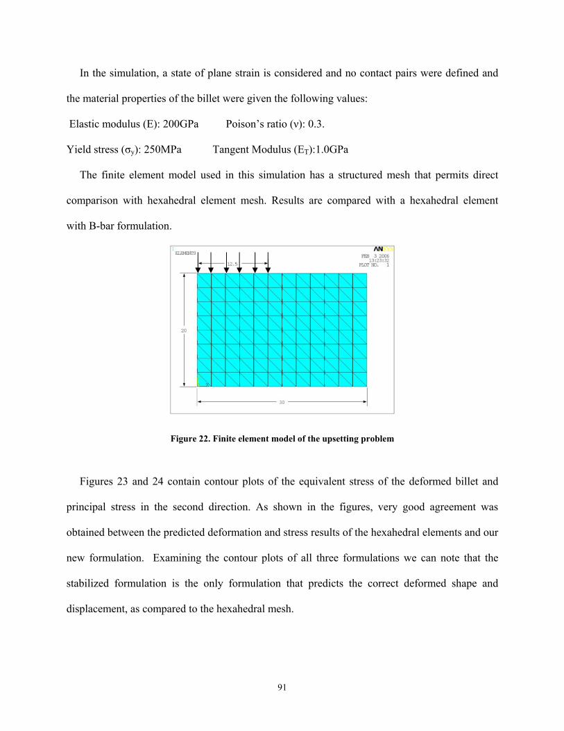
In the simulation, a state of plane strain is considered and no contact pairs were defined and
the material properties of the billet were given the following values:
The finite element model used in this simulation has a structured mesh that permits direct
comparison with hexahedral element mesh. Results are compared with a hexahedral element
with B-bar formulation.
hedral elements and our
ew formulation. Examining the contour plots of all three formulations we can note that the
abilized formulation is the only formulation that predicts the correct deformed shape and
isplacement, as compared to the hexahedral mesh.
Elastic modulus (E): 200GPa Poison’s ratio (ν): 0.3.
Yield stress (σy): 250MPa Tangent Modulus (ET):1.0GPa
Figure 22. Finite element model of the upsetting problem
Figures 23 and 24 contain contour plots of the equivalent stress of the deformed billet and
principal stress in the second direction. As shown in the figures, very good agreement was
obtained between the predicted deformation and stress results of the hexa
n
st
d
91
The mixed u/p formulation without stabilization predicts close values of equivalent stress but
when looking at the deformed shape it can be seen that the displacements are highly
underestimated, indicating severe volumetric locking. In fact the deformation of the mixed u/p
formulation predicts an upward direction of plastic flow which is totally different from the real
one. The pure displacement formulation also shows clear evidence of locking by inspection of
the deformed shape and high values of principal stress. The stabilization effect of the mixed
enhanced strain formulation is very obvious from the plots of the second principal stress which
show a smooth distribution in contrast to the polluted distribution of stresses obtained with the
mixed formulation without stabilization.
Even though the results are improved a lot compared with the other formulations, there are
still some differences when compared to the hexahedral ones. The only difference in the
predicted results relates to the deformation of the billet around the punch corner where the
tetrahedral model predicts a smaller slope between the punch face and the free surface than the
hexahedral model. In that area the mesh is highly distorted and the compressive stress
corresponding to that element is very high as compared to the hexahedral stress. We have to keep
ore it is
xpected that the stresses would have high values which consequently change the contour plot so
that the comp ral elements.
Because of these reasons, in Figures 23 and 24, (c) the equivalent stress and second principal
stress for hexahedral model was plotted using the same contour range as for the tetrahedral and
as it can be seen, our supposition that the singularity at the sharp corner is the only area that
differs from the reference plot was confirmed. The stabilized tetrahedral model shows a smooth
distribution with values similar to the hexahedral one everywhere except at that corner.
in mind though that any sharp corner represents a singularity for the stresses and theref
e
arison to hexahedral elements seems detrimental to the tetrahed
92
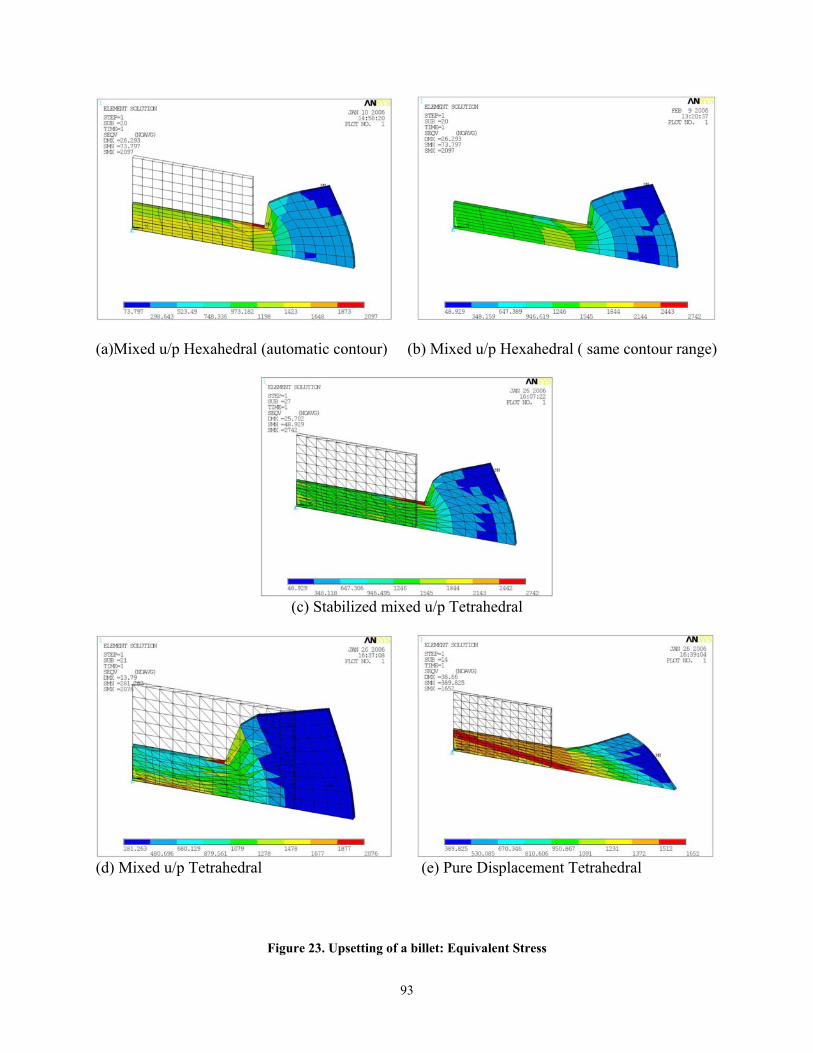
(b) Mixed u/p Hexahedral ( same contour range)
(c) Stabilized mix d u/p Tetrahedral
) Pure Displacement Tetrahedral
Figure 23. Upsetting of a billet: Equivalent Stress
(a)Mixed u/p Hexahedral (automatic contour)
e
(d) Mixed u/p Tetrahedral (e
93
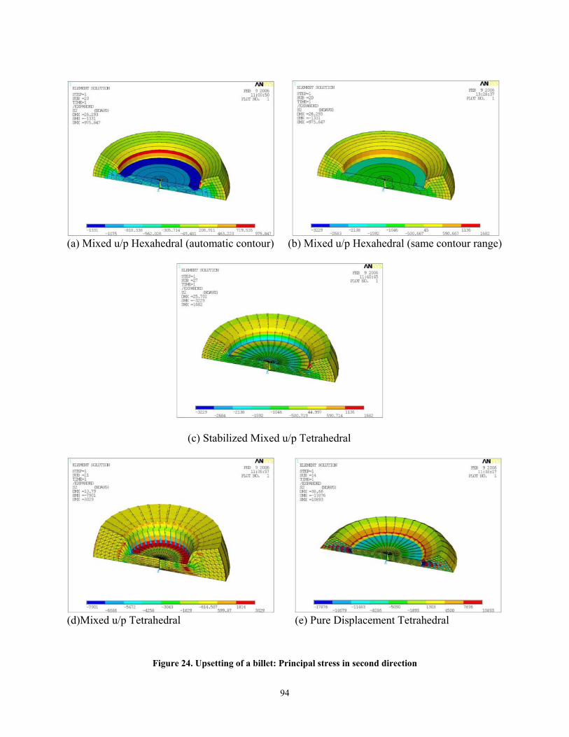
(a) Mixed u/p Hexahedral (automatic contour) (b) Mixed u/p Hexahedral (same contour range)
(c) Stabilized Mix Tetrahedral
(d)Mixed u/p Tetrahedral (e) Pure Displacement Tetrahedral
Figure 24. Upsetting of a billet: Principal stress in second direction
ed u/p
94
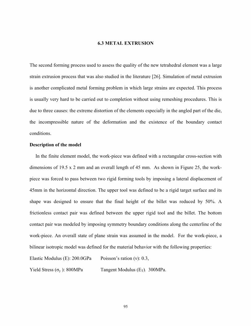
6.3 METAL EXTRUSION
The second forming process used to assess the quality of the new tetrahedral element was a large
strain extrusion process that was also studied in the literature [26]. Simulation of metal extrusion
is another complicated metal forming problem in which large strains are expected. This process
is usually very hard to be carried out to completion without using remeshing procedures. This is
Description of the model
In the finite element model, the work-piece was defined with a rectangular cross-section with
dimensions of 19.5 x 2 mm and an overall length of 45 mm. As shown in Figure 25, the work-
piece was forced to pass between two rigid forming tools by imposing a lateral displacement of
45mm in the horizontal direction. The upper tool was defined to be a rigid target surface and its
shape was designed to ensure that the final height of the billet was reduced by 50%. A
frictionless contact pair was defined between the upper rigid tool and the billet. The bottom
contact pair was modeled by imposing symmetry boundary conditions along the centerline of the
work-pie -piece, a
ilinear isotropic model was defined for the material behavior with the following properties:
Elastic Modulus (E): 200.0GPa
ield Stress (σy ): 800MPa Tangent Modulus (ET): 300MPa.
due to three causes: the extreme distortion of the elements especially in the angled part of the die,
the incompressible nature of the deformation and the existence of the boundary contact
conditions.
ce. An overall state of plane strain was assumed in the model. For the work
b
Poisson’s ration (ν): 0.3,
Y
95
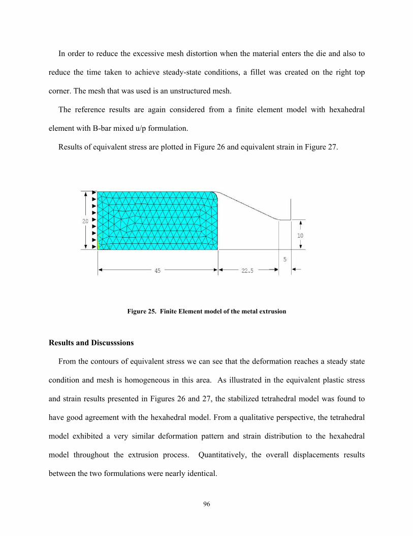
In order to reduce the excessive mesh distortion when the material enters the die and also to
reduce the time taken to achieve steady-state conditions, a fillet was created on the right top
corner. The mesh that was used is an unstructured mesh.
The reference results are again considered from a finite element model with hexahedral
element with B-bar mixed u/p formulation.
Figure 25. Finite Element model of the metal extrusion
Results and Discusssions From the contours of equivalent stress we can see that the deformation reaches a steady state
condition and mesh is homogeneous in this area. As illustrated in the equivalent plastic stress
and strain results presented in Figures 26 and 27, the stabilized tetrahedral model was found to
have good agreement w ective, the tetrahedral
ilar deformation pattern and strain distribution to the hexahedral
model throughout the extrusion process. Quantitatively, the overall displacements results
between the two formulations were nearly identical.
Results of equivalent stress are plotted in Figure 26 and equivalent strain in Figure 27.
ith the hexahedral model. From a qualitative persp
model exhibited a very sim
96
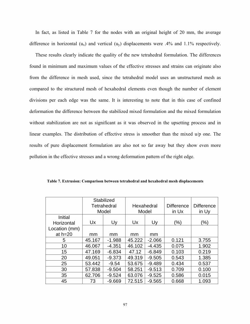
In fact, as listed in Table 7 for the nodes with an original height of 20 mm, the average
difference in horizontal (ux) and vertical (uy) displacements were .4% and 1.1% respectively.
These results clearly indicate the quality of the new tetrahedral formulation. The differences
found in minimum and maximum values of the effective stresses and strains can originate also
Tetrahedral Hexahedral Difference Difference
from the difference in mesh used, since the tetrahedral model uses an unstructured mesh as
compared to the structured mesh of hexahedral elements even though the number of element
divisions per each edge was the same. It is interesting to note that in this case of confined
deformation the difference between the stabilized mixed formulation and the mixed formulation
without stabilization are not as significant as it was observed in the upsetting process and in
linear examples. The distribution of effective stress is smoother than the mixed u/p one. The
results of pure displacement formulation are also not so far away but they show even more
pollution in the effective stresses and a wrong deformation pattern of the right edge.
Table 7. Extrusion: Comparison between tetrahedral and hexahedral mesh displacements
Stabilized
Model Model in Ux in Uy
Ux Uy Ux Uy (%) (%) Initial
Location (mm) Horizontal
at h=20 mm mm mm mm 5 45.167 -1.988 45.222 -2.066 0.121 3.755 10 46.067 -4.351 46.102 -4.435 0.075 1.902 15 47.169 -6.834 47.12 -6.849 0.103 0.219 20 49.051 -9.373 49.319 -9.505 0.543 1.385 25 53.442 -9.54 53.675 -9.489 0.434 0.537 30 57.838 -9.504 58.251 -9.513 0.709 0.100 35 62.706 -9.524 63.076 -9.525 0.586 0.015 45 73 -9.669 72.515 -9.565 0.668 1.093
97
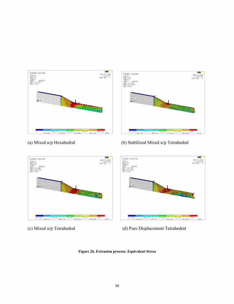
(a) Mixed u/p Hexahedral (b) Stabilized Mixed u/p Tetrahedral
(c) Mixed u/p Tetrahedral (d) Pure Displacement Tetrahedral
Figure 26. Extrusion process: Equivalent Stress
98
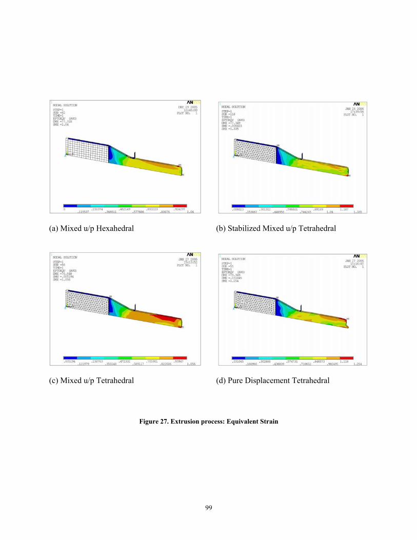
(b) Stabilized Mixed u/p Tetrahedral
Pure Displacement Tetrahedral
c
(a) Mixed u/p Hexahedral
(c) Mixed u/p Tetrahedral (d)
Figure 27. Extrusion pro ess: Equivalent Strain
99
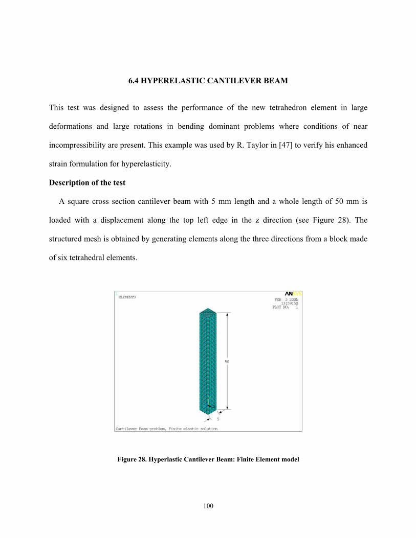
6.4 HYPERELASTIC CANTILEVER BEAM
This test was designed to assess the performance of the new tetrahedron element in large
deformations and large rotations in bending dominant problems where conditions of near
incompressibility are present. This example was used by R. Taylor in [47] to verify his enhanced
5 mm length and a whole length of 50 mm is
edge in the z direction (see Figure 28). The
ents along the three directions from a block made
Figure 28. Hyperlastic Cantilever Beam: Finite Element model
strain formulation for hyperelasticity.
Description of the test
A square cross section cantilever beam with
loaded with a displacement along the top left
structured mesh is obtained by generating elem
of six tetrahedral elements.
100
The material used is hyperelastic with a Neo-Hookean formulation defined by the following
two constants:
G=333.35MPa
d= 1/K = 1.2e-6
The reference finite element model is constructed from mixed u/p hexahedral elements with
an enhanced strain formulation because the problem is of a bending dominant type. As done
previously the stabilized formulation is pres together with the other two formulations,
mixed u/p and pure displacement, for comparison reasons. Contours of equivalent stress,
principal stress in the second direction and hydrostatic pressures are shown in Figures 29, 30 and
31. As illustrated in the contour plots, the stabilized enhanced formulation is clearly predicting a
deformed shape closest to the hexahedral finite element model (note that the final deformed
shape is almost horizontal). The mixed u/p formulation, in contrast, shows a much stiffer
n cking and
correctly predicts twisting of the beam instead of bending. In fact, the pure displacement
formulation in this erged substep are
abilized tetrahedral are similar with those of
hexahedral one and the values of these stresses are within 10 % error. It is noteworthy to mention
at even though we have the same number of nodes for both models, the number of tetrahedral
elements is six times larger than the number of hexahedral elements. In addition, the tetrahedral
elements have 4 degrees of freedom at each node while the hexahedral ones have only three (the
pressure is considered constant in this element).
As for the principal stress contour plots in Figure 30, the comparison is even more difficult
because it can be observed that even for the hexahedral elements the mixed enhanced strain
ented
response of the beam while the pure displaceme t formulation shows evidence of lo
in
case did not even converge, so only results at the last conv
shown. The equivalent stress contours of the st
th
101
formulation (Fig. 30(a)) and the B-bar (Fig. 30(b)) give different results, with the stabilized
tetrahedral compressive stress being closer to the compressive stress of the mixed enhanced
tress being closer to the B-bar formulation of the same elements. The
icz
ure distributions no longer
hexahedral and the tensile s
hydrostatic pressures are the most sensitive variables when considering locking. A special note
has to be made when examining those plots: due to the negative sign considered in the
interpolated pressure of the stabilized tetrahedral element as compared to the pressure calculated
from stresses of the hexahedral elements, the pressure degree of freedom is plotted with the signs
reversed. Therefore when looking at the pressure plots, the minimum pressure of the tetrahedral
model is -340 and the maximum pressure is 205. If compared to the hexahedral model, we can
see that the maximum pressure is in very good agreement (202) while the minimum pressure
shows a peak value. This peak value in the pressures induced by the compressive stresses was
noted also by Onate in his results while applying the FIC method [36] and also by Zienkiew
and Taylor in [49].
Overall the stability is improved since the principal stress and press
show the spurious oscillations observed in standard and mixed u/p formulations.
102
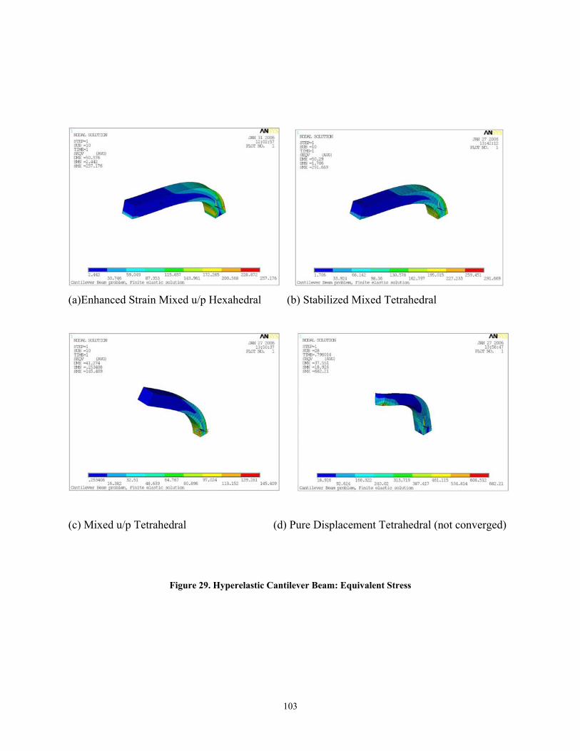
103
)Enhanced Strain Mixed u/p Hexahedral (b) Stabilized Mixed Tetrahedral
(a
(c) Mixed u/p Tetrahedral (d) Pure Displacement Tetrahedral (not converged)
Figure 29. Hyperelastic Cantilever Beam: Equivalent Stress
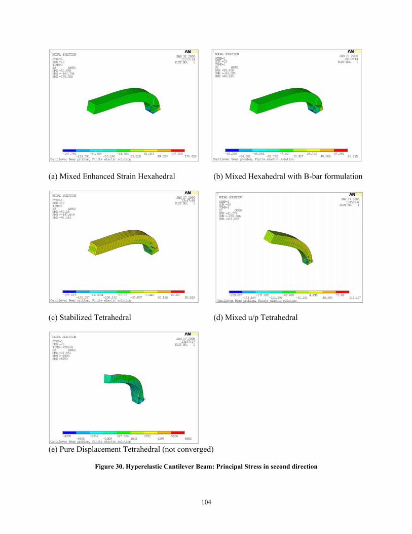
(a) Mixed Enhanced Strain Hexahedral (b) Mixed Hexahedral with B-bar formulation
(c) Stabilized Tetrahedral e trah
ent Tetrahedral (not converged)
Figure 30. Hyperelastic Cantilever Beam: Principal Stress in second direction
(d) Mix d u/p Te edral
(e) Pure Displacem
104
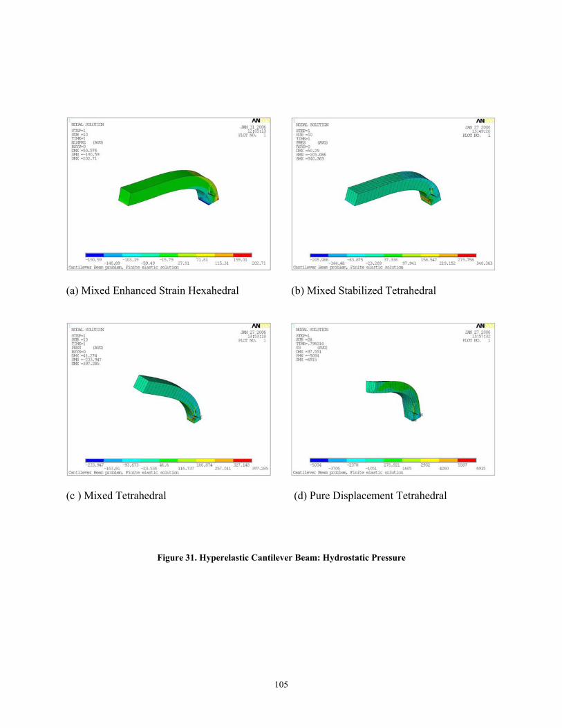
(b) Mixed Stabilized Tetrahedral
(d) Pure Displacement Tetrahedral
Beam: Hydrostatic Pressure
(a) Mixed Enhanced Strain Hexahedral
(c ) Mixed Tetrahedral
Figure 31. Hyperelastic Cantilever
105
7.0 CONCLUSIONS
7.1 SUMMARY
trahedral element, exhibit the phenomenon of
mpressibility are encountered during an analysis.
develop a robust and accurate low-order solid
tter performance than the existing ones. This was
t that could be used to solve general large
ons that can incorporate a wide range of
in the fact that analysts are bringing more geometric
quiring the development of algorithms that can
reasons, the newly developed element will be
with complicated geometries which can not be
the immediate expected fields of applications will
Reviewing the results presented in this dissertation, five different methods of stabilizing the
mixed linear displacement/linear pressure tetrahedral element were reviewed in Chapter 2. It was
concluded that under specific conditions they are all equivalent. The main question was which
one to choose and why. In Chapter 3, a new general formulation applicable to small and large
deformation and large rotations was presented.
Many finite elements, such as the linear te
volumetric locking when situations of near inco
The main goal of the present research was to
tetrahedral element that exhibits significantly be
primarily motivated by the absence of an elemen
deformation problems under incompressible conditi
nonlinear materials. Another motivation lies
details into finite element models, thereby re
readily interface with CAD models. For these two
useful in solving large finite element models
meshed with standard brick elements. One of
be metal forming.
106
The new solid tetrahedral element was formulated based on the principle of virtual work and
it was stabilized through an enhanced strain derived from a bubble function. Two bubble
functions were studied and the results were found to be identical. This approach was chosen
among the five choices for the following reasons: it does not require material or mesh dependent
parameters, consistent in nonlinear analysis, reasonable stable and computationally efficient. The
mixed stabilized formulation together with other two formulations, (a non-stabilized mixed and a
standard pure displacement formulation), was implemented through a user-programmable
element that interfaces with the commercial finite element software ANSYS. The finite element
code uses the pre- and post- processing capabilities as well as the nonlinear solvers of ANSYS.
Aspects of the implementation were discussed in Chapter 4.
Several numerical investigations were carried out to verify the element formulation. Some
linear tests results were presented and discussed in Chapter 5 and some nonlinear tests with
mphasis on simulation of metal forming applications were presented in Chapter 6. The
hen they were available and in most cases by comparisons with a similar analysis carried out
with well known stabilize ANSYS. To assess the
proved performance of the mixed stabilized formulation, the results were compared to two
ther formulations. All numerical examples, both linear and nonlinear, demonstrated the
bustness, accuracy and improved performance of the new element in quasi and fully
compressible problems that involve large deformation. In these problems consistent
improvement was obser the pure displacement
rmulations. This observation was motivated by the improved stress distributions, improved
accuracy of the displacements, and closer results to the stabilized hexahedral elements. Even
e
verification of the new formulation was assessed through comparisons with theoretical results
w
d hexahedral element already existing in
im
o
ro
in
ved over the mixed u/p without stabilization and
fo
107
though the new element behaved correctly in bending dominant problems in both linear and
nonlinear analyses, it still showed shear locking in pure bending problems.
e new lower order tetrahedral element lies within its ability to provide
are creating increasingly complex components.
7.2 SUGGESTIONS FOR FUTURE WORK
The robustness of the newly developed element needs to be further explored by performing
various analyses using different deformation conditions and a wide range of nonlinear materials.
Four major research directions can be foreseen for a future development of the proposed
element.
1. An interesting future work would be the investigation of the new formulation when using
anisotropic materials. The formulation should work since no specific assumptions were
made on the
2. The choice of bubble functions remains an open investigation area, since the only two
here produced identical results. Zienkiewicz and Taylor [49] recently used a
unctions and obtained promising results. This indicates that
stabilization can further be improved by the choice of bubble functions.
3. Another issue that was not thoroughly studied in the present study is the influence of the
mesh alignment on the results. This was detected in several papers and needs to be further
The importance of th
large deformation analysis capabilities for metal forming problems where the automatic
generation of hexahedral elements is not possible, especially when rezoning procedures are
applied. Such technology could prove to be an important step in the advancement of simulating
metal forming processes that
choice of the material constitutive law.
investigated
set of three bubble f
108
addressed since it can influence the results obtained after automatic generation of
elements during different remeshing techniques.
4. The present formulation was developed for static analyses but it can be extended to
transient analyses as well. This can be accomplished because the enhanced term is a
strain (not a displacement) which will not affect the inertial terms. It would be interesting
to test the performance of the stabilized tetrahedral element in static analyses with body
forces.
109
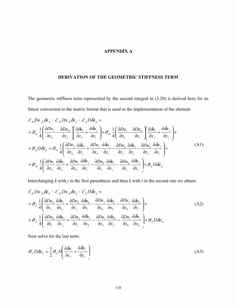
APPENDIX A
DERIVATION OF THE GEOMETRIC STIFFNESS TERM
The geometric stiffness term represented by the second integral in (3.20) is derived here for its
future conversion to the matrix format that is used in the implementation of the element.
ijiji
j
i
k
j
i
i
k
i
j
k
i
j
i
k
ijk
i
j
j
k
j
i
j
k
i
j
k
j
j
i
k
jikijij
i
j
jikik
i
j
jjk
jik x
uxu
xDu
xDu
xu
xu
xDu
xDu δδδδ ikiik
ijijijikjkijjkik
Dxu
xDu
xu
xDu
xu
xDu
xu
xDu
xu
xDu
xu
xDu
xu
xDu
xu
xDu
D
DDD
δεσδδδδσ
δδδδσδεσ
σσ
δεσδεωσδεωσ
+⎟⎟⎠
⎞⎜⎜⎝
⎛∂∂
∂∂
−∂∂
∂∂
−∂∂
∂∂
+∂∂
∂∂
+⎟⎟⎠
⎞⎜⎜⎝
⎛∂∂
∂∂
−∂∂
∂∂
−∂∂
∂∂
+∂∂
∂∂
=
+⎟⎜ +⎟⎜ −+⎟⎜ +⎟⎜ −=
=
⎟⎠
⎞⎜⎝
⎛∂∂
∂∂
⎟⎠
⎞⎜⎝
⎛∂∂
∂∂
⎟⎠
⎞⎜⎝
⎛∂∂
∂∂
⎟⎠
⎞⎜⎝
⎛∂∂
∂∂
++
41
41 (A1)
terchanging k with j in the first parenthesis and then k with i in the second one we obtain:
41
41
+
+
In
ijijk
j
k
i
j
k
k
i
k
j
i
k
j
k
i
kji
i
k
k
j
k
i
k
j
i
k
j
k
k
i
j
kij
ijijijikjkijjkik
Dxu
xDu
xu
xDu
xu
xDu
xu
xDu
xu
xDu
xu
xDu
xu
xDu
xu
xDu
DDD
δεσδδδδσ
δδδδσ
δεσδεωσδεωσ
+⎟⎟⎠
⎞⎜⎜⎝
⎛∂∂
∂∂
−∂∂
∂∂
−∂∂
∂∂
+∂∂
∂∂
+⎟⎟⎠
⎞⎜⎜⎝
⎛∂∂
∂∂
−∂∂
∂∂
−∂∂
∂∂
+∂∂
∂∂
=++
41
41 (A2)
ow solve for the last term:
=
+
N
⎟⎟⎠
⎞⎜⎜⎝
⎛∂∂
+∂∂
=i
j
j
iijijij x
uxu
DDδδσδεσ
21 (A3)
110
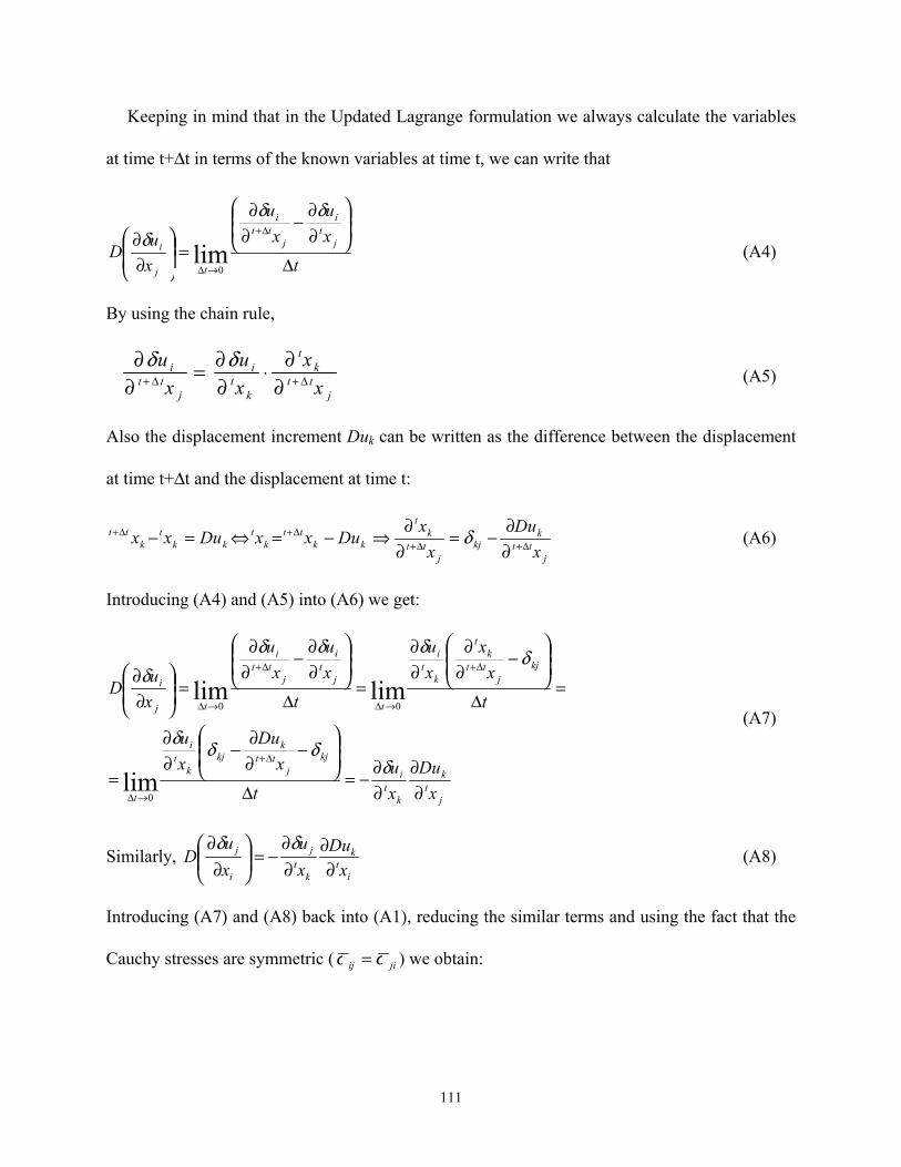
Keeping in mind that in the Updated Lagrange formulation we always calculate the variables
at time t+∆t in terms of the known variables at time t, we can write that
t
xu
xu
xu
D jt
i
jtt
i
tj
i
∆
⎟⎟⎠
⎞⎜⎜⎝
⎛
∂∂
−∂∂
=⎟⎟⎠
⎞⎜⎜⎝
⎛∂∂ ∆+
→∆
δδδ
lim0
(A4)
By using the chain rule,
jttk
ti
tti
xxx ∆+∆+ ∂⋅
∂=
∂ t
kj
xuu ∂∂∂ δδ (A5)
Also the displacement increment Duk can be written as the difference between the displacement
at time t+∆t and the displacement at time t:
jtt
kkj
jttk
t
kktt
kt
kkt
ktt
xDu
xx
DuxxDuxx ∆+∆+∆+∆+
∂∂
−=∂∂
⇒−=⇔=− δ (A6)
Introducing (A4) and (A5) into (A6) we get:
jt
k
kt
i
kjj
ttk
kjk
ti
t
kjj
ttk
t
kt
i
t
jt
i
jtt
i
tj
i
xDu
xu
t
xDuu ⎛ ∂∂δ
(A7)
x
t
xx
xu
t
xu
xu
xu
∂∂
∂∂
−=∆
⎟⎟⎠
⎞⎜⎜⎝
−∂
−∂
=
=∆
⎟⎟⎠
⎞⎜⎛ −∂
∂∂
=∆
⎟⎟⎠
⎞⎜⎜⎝
⎛
∂∂
−∂∂
=⎟⎟⎠
⎞⎜⎜⎝
⎛∂∂
∆+
→∆
∆+
→∆
∆+
→∆
δδδ
δδδδδ
lim
limlim
0
00
imilarly,
⎜⎝ ∂D
it
k
kt
j
i
j
xDu
xu
xu
D∂∂
∂∂
−=⎟⎟⎠
⎞⎜⎜⎝
⎛∂∂ δδ
(A8)
troducing (A7) and (A8) back into (A1), reducing the similar terms and using the fact that the
auchy stresses are symmetric (
S
In
jiij σσ = ) we obtain: C
111
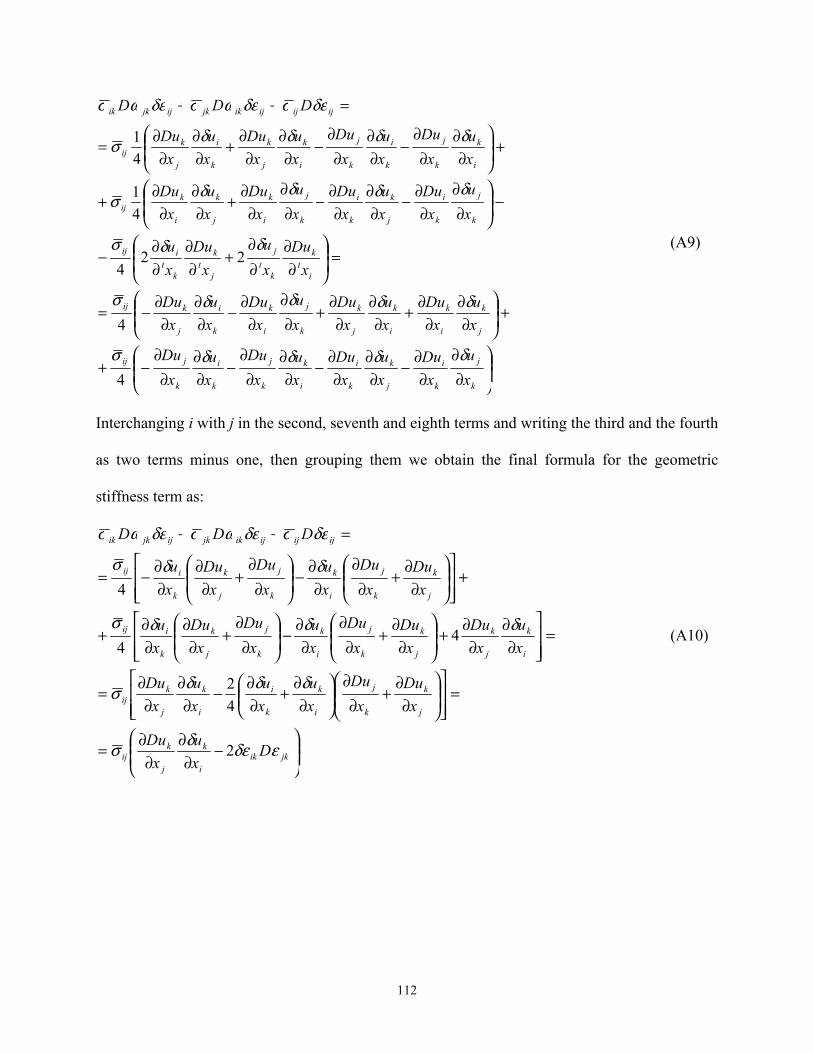
⎟⎟⎠
⎞⎜⎜⎝
⎛∂∂
∂∂
−∂∂
∂∂
−∂∂
∂∂
−∂∂
∂∂
−+
+⎟⎟⎠
⎞⎜⎜⎝
⎛∂∂
∂∂
+∂∂
∂∂
+∂∂
∂∂
−∂∂
∂∂
−=
=⎟⎟⎠
⎞⎜⎜⎝
⎛
∂∂
∂∂
+∂∂
∂∂
−
−⎟⎟⎠
⎞⎜⎜⎝
⎛∂∂
∂∂
−∂∂
∂∂
−∂∂
∂∂
+∂∂
∂∂
+
+⎟⎟⎠
⎞⎜⎜⎝
⎛∂∂
∂∂
−∂∂
∂∂
−∂∂
∂∂
+∂∂
∂∂
=
=++
k
j
k
i
j
k
k
i
i
k
k
j
k
i
k
jij
j
k
i
k
ij
k
k
j
i
k
k
i
j
kij
it
k
kt
j
jt
k
kt
iij
k
j
k
i
j
k
k
i
k
j
i
k
j
k
i
kij
i
k
k
j
k
i
k
j
i
k
j
k
k
i
j
kij
ijijijikjkijjkik
xu
xDu
xu
xDu
xu
xDu
xu
xDu
xu
xDu
xu
xDu
xu
xDu
xu
xDu
xDu
xu
xDu
xu
xu
xDu
xu
xDu
xu
xDu
xu
xDu
xu
xDu
xu
xDu
xu
xDu
xu
xDu
DDD
δδδδσ
δδδδσ
δδσ
δδδδσ
δδδδσ
δ
k
εσδεωσδεωσ
4
4
224
41
41
(A9)
Interchanging i with j in the second, seventh and eighth terms and writing the third and the fourth
as two terms minus one, then grouping them we obtain the final formula for the geometric
stiffness term as:
⎟⎟⎠
⎞⎜⎜⎝
⎛−
∂∂
∂∂
=
=⎥⎥⎦
⎤
⎢⎢⎣
⎡⎟⎟⎠
⎞⎜⎜⎝
⎛∂∂
+∂∂
⎟⎟⎠
⎞⎜⎜⎝
⎛∂∂
+∂∂
−∂∂
∂∂
=
=⎥⎥⎦
⎤
⎢⎢⎣
⎡
∂∂
∂∂
+⎟⎟⎠
⎞⎜⎜⎝
⎛∂∂
+∂∂
∂∂
−⎟⎟⎠
⎞⎜⎜⎝
⎛∂∂
+∂∂
∂∂
+
+⎥⎤
⎢⎡
⎟⎟⎞
⎜⎜⎛ ∂
+∂
−⎟⎟⎞
⎜⎜⎛ ∂
+∂∂
−=⎥⎦⎢⎣ ⎠⎝ ∂∂
∂∂⎠⎝ ∂∂∂
=++
jkiki
k
j
kij
j
k
k
j
i
k
k
i
i
k
j
kij
i
k
j
k
j
k
k
j
i
k
k
j
j
k
k
iij
jkikjk
ijijijikjkijjkik
Dxu
xDu
xDu
xDu
xu
xu
xu
xDu
xu
xDu
xDu
xDu
xu
xDu
xDu
xu
xD
xxxxx
DDD
εδεδσ
δδδσ
δδδσ
δ
kjkjkiij uDuuDuDuu δδσ
εσδεωσδεωσ
2
42
44
4
(A10)
112
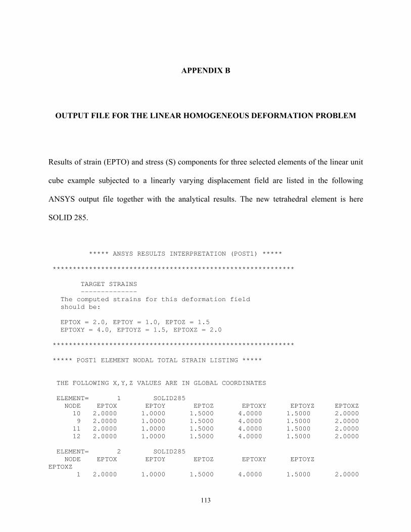
APPENDIX B
OUTPUT FILE FOR THE LINEAR HOMOGENEOUS DEFORMATION PROBLEM
Results of strain (EPTO) and stress (S) compo for three selected elements of the linear unit
cube example subjected to a linearly varying displacement field are listed in the following
ANSYS output file together with the analytical results. The new tetrahedral element is here
SOLID 285.
***** ANSYS RESULTS INTERPRETATION (POST1) ***** ************************************************************
The computed strains for this deformation field should be: EPTOX = 2.0, EPTOY = 1.0, EPTOZ = 1.5 EPTOXY = 4.0, EPTOYZ = 1.5, EPTOXZ = 2.0 ************************************************************ ***** POST1 ELEMENT NODAL TOTAL STRAIN LISTING ***** THE FOLLOWING X,Y,Z VALUES ARE IN GLOBAL COORDINATES ELEMENT= 1 SOLID285 NODE EPTOX EPTOY EPTOZ EPTOXY EPTOYZ EPTOXZ
4.0000 1.5000 2.0000 11 2.0000 1.0000 1.5000 4.0000 1.5000 2.0000 12 2.0000 1.0000 1.5000 4.0000 1.5000 2.0000 ELEMENT= 2 SOLID285 NODE EPTOX EPTOY EPTOZ EPTOXY EPTOYZ PTOXZ 1 2.0000 1.0000 1.5000 4.0000 1.5000 2.0000
nents
TARGET STRAINS --------------
10 2.0000 1.0000 1.5000 4.0000 1.5000 2.0000 9 2.0000 1.0000 1.5000
E
113
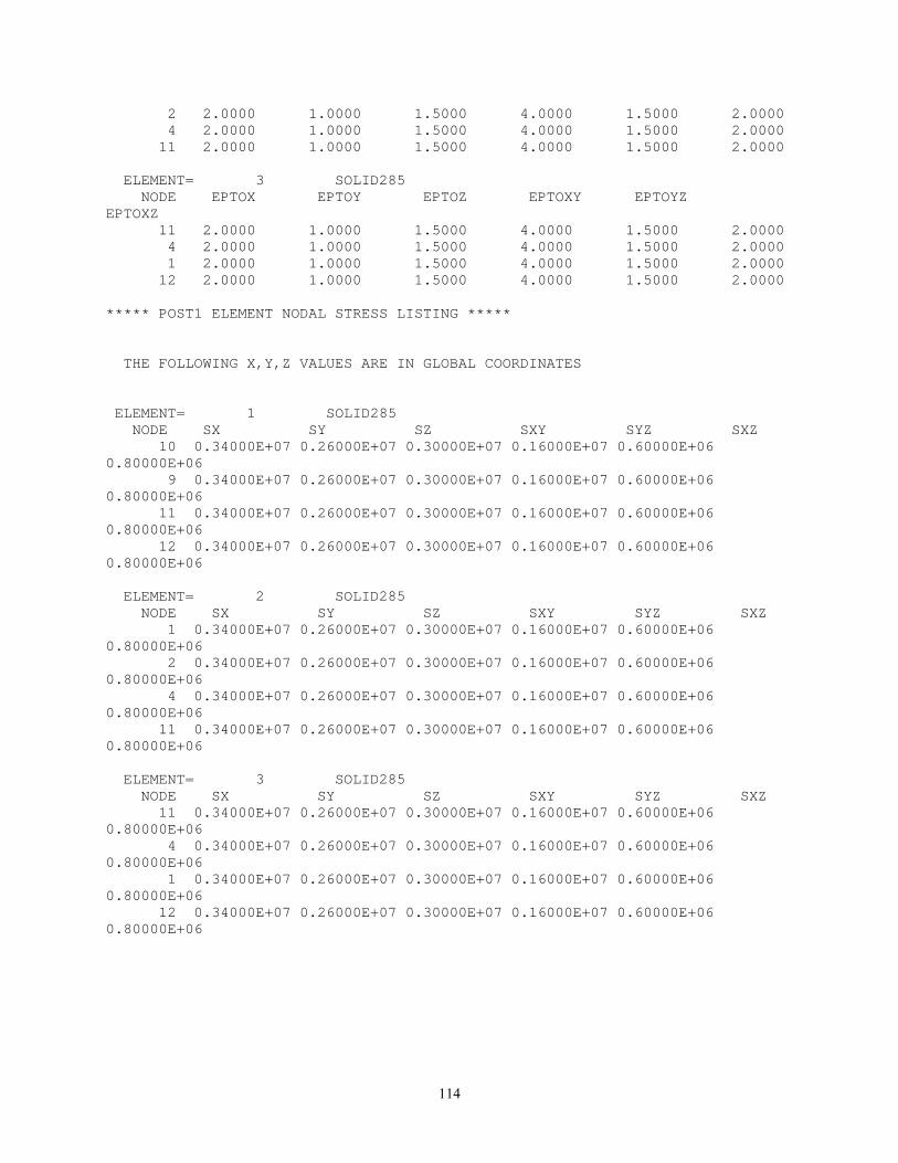
2 2.0000 1.0000 1.5000 4.0000 1.5000 2.0000 4 2.0000 1.0000 1.5000 4.0000 1.5000 2.0000 11 2.0000 1.0000 1.5000 4.0000 1.5000 2.0000 ELEMENT= 3 SOLID285 NODE EPTOX EPTOY EPTOZ EPTOXY EPTOYZ EPTOXZ 11 2.0000 1.0000 1.5000 4.0000 1.5000 2.0000 4 2.0000 1.0000 1.5000 4.0000 1.5000 2.0000 1 2.0000 1.0000 1.5000 4.0000 1.5000 2.0000 12 2.0000 1.0000 1.5000 4.0000 1.5000 2.0000 ***** POST1 ELEMENT NODAL STRESS LISTING ***** THE FOLLOWING X,Y,Z VALUES ARE IN GLOBAL COORDINATES ELEMENT= 1 SOLID285 NODE SX SY SZ SXY SYZ SXZ 10 0.34000E+07 0.26000E+07 0.30000E+07 0.16000E+07 0.60000E+06 0.80000E+06 9 0.34000E+07 0.26000E+07 0.30000E+07 0.16000E+07 0.60000E+06 0.80000E+06 11 0.34000E+07 0.26000E+07 0.30000E+07 0.16000E+07 0.60000E+06 0.80000E+06 12 0.34000E+07 0.26000E+07 0.30000E+07 0.16000E+07 0.60000E+06 0.80000E+06 ELEMENT= 2 SOLID285 NODE SX SY SZ SXY SYZ SXZ 1 0.34000E+07 0.26000E+07 0.30000E+07 0.16000E+07 0.60000E+06
.80000E+06 4 0.34000E+07 0.26000E+07 0.30000E+07 0.16000E+07 0.60000E+06 0.80000E+06 11 0.34000E+07 0.26000E+07 0.30000E+07 0.16000E+07 0.60000E+06 0.80000E+06 ELEMENT= 3 SOLID285 NODE SX SY SZ SXY SYZ SXZ 11 0.34000E+07 0.26000E+07 0.30000E+07 0.16000E+07 0.60000E+06 0.80000E+06 4 0.34000E+07 0.26000E+07 0.30000E+07 0.16000E+07 0.60000E+06 0.80000E+06 1 0.34000E+07 0.26000E+07 0.30000E+07 0.16000E+07 0.60000E+06 0.80000E+06 12 0.34000E+07 0.26000E+07 0.30000E+07 0.16000E+07 0.60000E+06 0.80000E+06
0.80000E+06 2 0.34000E+07 0.26000E+07 0.30000E+07 0.16000E+07 0.60000E+06 0
114
BIBLIOGRAPHY
1. ABAQUS Manual. Hibbitt, Karlsson and Sorensen:1080 Main Street, Pawtucket, RI, 02860, USA, 2003.
2. ANSYS Release 10.0 Theory Verification Manual, Canonsburg, PA, USA :ANSYS Inc.,
2005.
3. D.N. Arnold, F.Brezzi, and M. Fortin. A stable finite element for the Stokes equations. Calcolo, 21:337-344,1984.
4. Babuška I. Error bounds for finite element methods. Numer.Math., 16:322-333, 1971.
5. C. Baiocchi, F.Brezzi. Virtual bubbles and Galerkin-least-squares type methods.
Comput.Methods Appl. Mech. Engnrg. 105:125-141, 1993.
6. Klaus-Jurgen Bathe. Finite element procedures. Prentice-Hall, Upper Saddle River, NJ, 1996.
element e C m u 469-482,
2000.
8. Ted Belytschko, Wing Kam Liu, Brian Moran. Nonlinear finite elements for continua and structures. Chi
9. F.H.Bertrand, M.R.Gadbois, and P.A.Tanguy. Tetrahedral elements for fluid flow. Int. J.
Numer. Meth. Engng. 33:1251-1267,1992.
10. F.Brezzi, M.O.Bristeau,L.P.Franca, M.M.Gilbert Rogé. A relationship between stabilized finite element methods and the Galerkin method with bubble functions. Comput.Methods Appl. Mech. Engnrg. 96:117-129, 1992.
11. F.Brezzi, J.Pitkäranta. On the stabilization of finite element approximations of the Stokes
problem. In W.Hackbusch,editor, Efficient solution of Elliptic problems, Notes on Numerical Fluid Mechnaics, vol.10,Vieweg, Wiesbaden, 1984.
12. F.Brezzi, L.P.Franca, T.J.R.Hughes, A.Russo. Comput. Methods Appl. Mech.
Engnrg. 145:329-339, 1997.
7. S.R. Beissel, G.R.Johnson. Large deformation triangular and tetrahedral
formulations for unstructured mesh s. o p t. Methods Appl. Mech. Engnrg. 187:
chester, England; New York : John Wiley, c2000.
∫= gb .
115
13. P.A.J.Van Den Bogert, R.De Boerst, G.T Luiten, and J.Zeilkmaker. Robust finite elements for 3D-analysis of rubber-like materials. Engineering Computations 8:3-17, 1991.
14. U.Brink, E.Stein. On some mixed finite elem for incompressible and nearly
incompressible finite elasticity. 19:105-119, 1996.
15. J.Bonet, H. Marriott and O.Hassan. An averaged nodal deformation gradient linear tetrahedral element for large strain explicit dynamics applications. Commun. Numer. Meth. Engng; 17:551-561, 2001.
16. J. Bonet and R.D.Wood. Nonlinear continuum mechanics for finite element analysis.
C bridge University Press, 1997.
18.
Engrng; 47:1549-1568, 2000.
2
ent methods Computational mechanics
am
17. M.Cervera, M.Chiumenti, Q. Valverde, C.A. de Saracibar, Mixed linear/linear simplicial elements for incompressible elasticity and plasticity. Comput. Methods Appl. Mech. Engnrg. 192:5249-5263, 2003.
M. Chiumenti, Q. Valverde, C Agelet de Saracibar, M.Cervera. A stabilized formulation for incompressible plasticity using linear triangles and tetrahedra. International Journal of Plasticity 20:1487-1504, 2004.
19. M. Chiumenti, Q. Valverde, C Agelet de Saracibar, M.Cervera. A stabilized formulation for
incompressible elasticity using linear displacement and pressure interpolations. Comput. Methods Appl. Mech. Engnrg. 191:5253-5264, 2002.
20. R. Codina. Stabilized finite element approximation of transient incompressible flows using
orthogonal subscales. Comput.Methods Appl. Mech. Engnrg. 191:4295-4321, 2002.
21. C.R.Dohrmann, S.W.Key, M.W.Heinstein and J .Jung. A least-squares approach for uniform straintriangular and tetrahedral finite elements. Int. J. Numer. Meth. Engrng; 42:1181-1197, 1998.
22. C.R.Dohrmann, S.W.Key, M.W.Heinstein, J.Jung and W.R. Witkowski. Node-based
uniform strain elements for three-node triangular and four-node tetrahedral meshes. Int. J. Numer. Meth.
3. L.P Franca, C. Farhat. On the limitations of bubble functions. Comput.Methods Appl. Mech.
Engnrg. 117:225-230, 1994.
24. L.P Franca, C. Farhat. Bubble functions prompt unusual stabilized finite element methods. Comput.Methods Appl. Mech. Engnrg. 123:299-308, 1995.
25. L.P.Franca, S.P.Oliveira. Pressure bubble stabilization features in the Stokes problem.
Comput.Methods Appl. Mech. Engnrg. 192:1929-1937, 2003.
116
2methods. Int. J. Numer. Meth. Engrng. 44:1397-1428, 1999.
27. T.J.R Hughes and J. Winget. Finite rotations effects in numerical integration of rate
1867,1980.
28. T.J.R. Hughes. The finite element method: Linear Static and Dynamic Analysis. Prentice –
computational fluid dynamics: V. Circumventing the Babuska-Brezzi condition: A stable
inerpolations. Comput.Methods Appl. Mech. Engnrg. 59:85-99, 1986.
30. T.J.R.Hughes. Multiscale phenomena:Green’s functions, the Dirichlet-to-Neumann
Comput.Methods Appl. Mech. Engnrg. 127:387-401, 1995.
31. O. Klaas, A. Maniatty, M.S.Shephard. A stabilized mixed finite element method for finite
Appl. Mech. Engnrg. 180:65-79, 1999.
32. R.M.McMeeking and J.Rice. Finite-element formulations for problems of large elastic-
introduction. Comput. Methods Appl. Mech. Engnrg. 192:3043-3059, 2003.
34. Eugenio Oñate. Possibilities of finite calculus in computational mechanics. Int. J.Numer.
finite calculus. Engineering Computations 20(5/6):629-658, 2003.
36. E. Oñate, J.Rojek, R.L.Taylor and O.C.Zienkiewicz. Finite Calculus formulation for
59:1473-1500, 2004.
37. M.Pastor, M.Quecedo, and O.C.Zienkiewicz. A mixed displacement-pressure formulation
Comput. Methods Appl. Mech. Engnrg. 68:205-227,1988.
6. M.S.Gadala and J.Wang. Simulation of metal forming processes with finite element
constitutive equations arising in large-deformation analysis. Short Communications: 1862-
Hall, Englewood Cliffs NJ, 1987
29. T.J.R. Hughes, L.P.Franca, and M.Balestra. A new finite element formulation for
Petrov-Galerkin formulation of the Stokes problem accommodating equal-order
formulation, subgrid scale models, bubbles and the origins of stabilized methods.
elasticity. Formulation for linear displacement and pressure interpolation. Comput. Methods
plastic deformation. Int.J.Solids Structures, 11:601-616, 1975.
33. Eugenio Oñate. Multiscale computational analysis in mechanics using finite calculus: an
Meth. Engng. 60; 255-281, 2004.
35. E.Oñate, R.L.Taylor, O,C.Zienkiewicz, J.Rojek. A residual correction method based on
incompressible solids using linear triangles and tetrahedra. Int. J.Numer. Meth. Engng.
for numerical analysis of plastic failure. Computers & Structures, vol.62, no.1:13-23, 1997.
38. Roger Pierre. Simple C0 approximations for the computation of incompressible flows.
117
39. Roger Pierre. Optimal selection of the bubble functions in the stabilization of the P1-P1
1224, 1995. element for the Stokes problem. SIAM Journal on Numerical Analysis, vol.32, no.4:1210-
4
in J2 solids. Comput.Methods Appl. Mech. Engnrg. 188:145-163, 2000.
41. J.Rojek, O.C.Zienkiewicz, E.Oñate, R.L.Taylor. Simulation of metal forming using new
et.al.(eds)©Balkema, Rotterdam, 2000.
42. J.Rojek, O.C.Zienkiewicz, E.Oñate, E.Postek. Advances in FE explicit formulation for echnology 119:41-
47, 2001.
43. Alessandro Russo. Bubble stabilization of finite element methods for the linearized incompressible Navier-Stokes equations. Comput. Methods Appl. Mech. Engnrg. 132:335-343, 1996.
44. David Silvester. Optimal low-order finite element methods for incompressible flow. Comput. Methods Appl. Mech. Engnrg. 111:357-368, 1994.
46. I.M. Smith and D.V. Griffiths. Programming the finite element method. John Wiley &Sons,
Taylor. A mixed-enhanced formulation for tetrahedral finite elements. Int. J.Numer. Meth. Engng. 47:205-227, 2000.
48. P.Thoudtireddy, J.F. Molinari, E
el
49. O ethod, vol.1- The Basis, McGraw-Hill, London,5th edition,2000.
0. M.Quecedo, M. Pastor, O.C.Zienkiewicz. Enhanced linear triangle for plasticity problems
formulation of triangular and tetrahedral elements. Metal Forming, Pietrzyk
simulation of metal forming processes. Journal of Materials Processing T
45. David Silvester. Stabilized mixed finite element methods. Numerical Analysis Report
No.262, August 1995.
3rd edition, 1997.
47. R.L.
.A.Repetto and M.Ortiz. Tetrahedral composite finite ements. Int. J. Numer. Meth. Engng. 53:1337-1351, 2002.
.C. Zienkiewicz and R. Taylor. The finite element m
118