v

FINITE ELEMENT FORMULATION OF NONLINEAR BOUNDARY-VALUE PROBLEMS

J. T. Oden

1

FINITE ELEMENT FORMULATION OF NONLINEAR BOUNDARY-VALUE PROBLEMS

J. T. Oden*

SUMMARY

The application of the finite element method to a large class ofnonlinear operator equations is considered. Some of the previous con-clusions concerning convergence for linear positive definite operatorsare reviewed and extended to nonlinear potential operators. Examplesare given in which the method is applied to representative nonlinearpartial differential equations and integral equations.

1. INTRODUCTION

.It is often the case with the approximate methods of mathematical

analysis that their practical value is established by numerous examples

long before their theoretical basis or their limitations are completely

understood. The finite-element method is no exception. While the method

has·been applied successfully to a wide range of lirear and nonlinear

problems over the past 15 or 80 years, available criteria for convergence

or for the selection of acceptable local finite element approximations

appear to he valid only for n rather narrow class of linear operators.

Moreover, the theoretical basis for finite-element approximations of non-

linear problems is developed to a far less extent than that for linear

problems.

The present lecture, which represents a revision and elaboration of

a forthcoming paper (1], concerns the application of the method of finite

elements to the approximate solution of certain nonlinear boundary-value

problems. We discuss the concept of potential operators and Galerkin's

method for nonlinear operators, and we elaborate on the application of

*Professor and Chairman, Department of Engineering Mechanics, TheUniversity of Alabama in Huntsville

2

Vainberg's Theorem [21 to the construction of variational principles

corresponding to given nonlinear houndary-value problcms. Concerning

the question of convergcnce, we limlt oursclves to elliptic-type opera-

tors for which a definite minimum principle exists; hut we nre ahle to

show that the completeness criteria of Oliveira (3] Lind their generaliza-

tions presented by Oden [41 for linear prohlems also upply tD this class

of nonlinear prohlems. Finally, Wc cite examplcs to illustrate npplicn-

tions of the theory.

2. SOME CONCEPTS ON GENERAL VARIATIONAL METHODS FOR NONLINEAR EQUATIC:NS

Nonlinear Operators. Many important problems in mathematical physics

are ~haracterized by equations of the form

@(u(x)] = 0 (2.1 )

where @ is a nonlinear operator and u(x) is some [unction of position

x in a region b-l. of EucJ idean sp:lce. The equation (2. I) is to be satis-

fied in the interior of ~ and on the houndades oR U(~) is required to

satisfy certain boundary conditions of the form

a[u(~)]= a (2.2)

where ~ is also a nonlinear operator. In both (2.1) and (2.2), pres-

cribed functions can appear, so that neither equation is to imply

'~omogeneousH conditions as in linear problems. Generally, we shall

aSSume in the followin~ that W, is a subre~ion of k-dimensim al Euc lidean

space and that ~ = (Xl,X~,•••,Xk)'

Since our primary concern shall he the construction of finitc-

element models of (2.1) (and (2.2», it is naturnl to question whether

3

or not it is possible to construct :1 variational statement of the problem

(2.1); that is, can We find a functional K(u) which assumes [) stationary

value at the solutions of (2.1), assuming that (2.2) is satisfied?

Fortunately, Wl' shall rind that the :JI1Swer to this question iH afrirma-

tive for a wide class or important Jlonlinear integral t~quations.

Derivatives of Operators. SUpPOs(~ that the oper.1tor (j carri(~s clunlents

from a linear vector space {-{into another linear spacu if. The el ell1ents

of ..{ and 'If are func tions 0 f some c lass de fined on ~ + o~-l.and the \1sua 1

properties of linear vector spaces hold (Le. Q'Ul(~) + Su:;!(~) (£.<, where

ct, 8 are scalars and Ul'U~ (<A., etc.). Suppose also that it is possible

to define on 'LA. and 'If a norm; that is, a real number associated with each

element u(v), denoted Ilu~1 (1Ivll), which obeys the norm axioms; lIull z 0, =

o iff u = 0, IIctldl = Ictl lIull, and lIu\ + u:111:s;"llulll + Ilu::ll. If U. and 'If

are complete, (Le., if Cauchy sequence8 (un} of clements converge in

the norms to limits Uo in ,.{ in the sense that 1illlilu R_ Uo II = 0, Uo (/;<),no"""

then they are referred to as nnnnch spaCt~H. Moreover, if llllll\@(u") -n·..."

@(uo) II = 0, then (} is said to be continuous at u •o

It is often possible to introduce in this [Ihstract setting of normed

spaces two alternate generalizations of the idea of differentiation and

of differentials: The Gateaux differential of @(u),denoted r~(u,h), and

the Frechet differential of 9(u), denoted 6(}(u,h), are defined by

and

lim \I i «() (u + cth) - @(u» - G<f( u , h) IIerO

o (2.3)

lim 11@(u+ h) - @(u) - 6@(u,h)11IIh!l-i()

o (2.4 )

4

Here h is an arbitrary element frum the interior of the domain f} 1.:-: U. of

(). The linear operators @(u)( ) am] (}'(u)( ), where (;(u) (h) = G(}(u,h)

and ()' (u) (h) = 6@(u,h), are called the Gat.~~ and Fre.chet deriyatives

of @ at u, respectively. Since it can be shown that if @(u) exists and

is continuous in the ncighhorhood of u then o@(u,h) exists [Ind is identi-

cally the same <IS 6@(u,h), we shall use the definitions and notatiuns of

(2.3) and (2.4) interckmgcably; i.e., we henceforth assume the existence

.and continuity of t?(u) •

To cite some silllple eX<IInples, suppose O(u) denotes the nonlinear

integral operator

@(u)

b

u(t) Ja(s,t)u(s)ds

a

a ~ s :S: b, where K(S,t) = K(t,S) is a given symmetric kcrnol. Then

@(u + h) - @(u)

a

= u(t) I a(s,t)h(s)ds

o

b

+ h(t) I a(s,t)u(s)ds

a

b

+ h(t) I a(s,t)h(s)ds

a

Thus, from ·(2.4) we ohtain for the Frechet differential of (}(u),

6@(u,h)

h

• U(t>I a(s,t)h(s)ds +

a

h

h(t) J a(s,t)u(s)ds

:1

which is linear in h.

As a second example, suppose

5

O(u) = '1'\1 - u;·

where ~u is tlw Lapl:tcian; i.c. 'Ii!\! '" u,11 = lY'u!oxldXl'i heing summcd

from 1 to k. Fo llowinl: the procedun' out lined ahovc, wc find in this

case, that

o<fl(u,h) = V"'h - 2uh

Functionals and Functional Derivatives. We now ndd to the structure Pll.'-

sented thusfar a hi linear mapping from 4 x 'If into the real numbers R that

associates with pairs of elements u (~, v ( ~ a real number, denoted

(u,v), that has the following properties:

(u,o)

(u,v)

(u,v)

(0, v)

O~u

= (v,u)

o

o or v = 0 (2.5)

These equations definc '-I linear [unctionn I. on i.,{ :md tlw reby identi fy ~

as the conjugate space o[ t,{: '!f = 'L(I~. In many applicat ions wc 0 ftlm find

that (..(is self-conjugate; i.e., i..{ = L{* and (; maps 'l.{ into itself. Like-

wise, in this case there is an important class of problcms in which it

is meaningful to add to (2.5) the stronger condition

(u,u) .: 0 (2.6)

the equality holding if and only if 1I = O.

Now n mapping K:"{ ~ R which :Issociates witl, elemcnts or 1{ rl.'ill

(or complex) numbers is called a functional. Tlw concept Or:l f\lllctional,

of course, plays an important role in variational calculus. Since K(u)

is also an operator on (..(, we can also spl.'nk of derivatives of functionals

in the same sense as (L.3). Indecd, for il given (;:ltC:IlIX dirrl!rl!ntlahlc

6

functional K(u), we call CO\Jlputc

J,~ (2.7)

or, equivnlently

oK (u, II) = ~ K (u + <xII) I0=0

(2.8)

Now oK(u,h) describes .:l linear functional on'L.( and thereby identifies

some sort of mapping of 'L.(into 'l{*. This mapping, say @(u), is called

the gradient of the functional K(u), and is denoted grad K(u). Further-

more, oK(u,h) is linear in h and grad K(u) can be defined so that

oK(u,h) is also linear in @(u). If we assume further that, for this bi-

linear operator conditions, (2.5) (.1nd possibly (2.6» hold, then we

can associate oK(u,h) directly with «(}(u),h), where @(u) is the gradient

of K(u). In summary, if K(u) posliesses ii.linear Gatc:lux differential

on ~ subset ~ C 'L.(, ~hcn the operator @(II) de fined .!.?}:

o(O(u),h) = lim en K(u + O'h)

()'-+ 0

is called the gradient of !.M, and we wri te @(u) = grad K(u).

(2.9)

To mention hriefly a few other definitions relative to r~teaux

differentiable function[lls, we cssentially adopt the fnmili[lr notions

of maxima, minima, and critical points of ordinary functions from ele-

mentary calculus. For example, a point u., ( j;) is a critical point of n

function,11 K(u) defined on ~ if gLld K(uo) 0, () being the zero elemcnt

in ~ c:\:t. Moreover, if K(u) 2. K(u ) for ;111 u (Ji) c.~, then u iii calledo 0 0

a global minimizer of K on /;)0 (or, if K(u) ~ K(u.,) for all u in g n /;),

g. being an open neighborhood of uo' then ul) is a local minimizer of K).

As expected, if Uo is a local minimizer of a Gateaux-differentiable

7

functional, then grad K(u ) = 0; that is, \J is a critical point of K(u).o 0

If the second Gateaux differential C4K(u,h,h) exists and is positive

definite (i.e. G:aK(u,h,h) > 0 for nIl h ( ~Q) nt <l critical point Uo of

K(u), then lIo is a proQer locallllinilllizer of K(II){i.c. K(u) > K(uo) for

If C:GK(u ,h,h) is posilive-sl'midcfinite at U,1I is:l lOCHlQ 0 "

minimizer of K(u). Fin,llly, if " .. is :J crl tic:! I point of K(II) nnll C:ilK

(u ,h,h) is neg,ltive definite or negative scmidl'rinitl', then u is;Io 0

proper maximizer or n local mnxillliz~~ of K(u), respectively.

We remark that second and higher-order differentials of functionaLs

(and other operators) can be obtained by repeated application of (2.3).

For example, the second Frechet (Gateaux) differential is

6<lK(u,h ,k)(3= lim dO' (6K(u + O'k,h) 1

cy-+ 0(2.10)

which is bilinear in hand k. If f>C!K(u,h,k) = 6:JK(u,k,h), we say that

K(u) is symmetric at u. By continueu diffcrcnti:ltiolls such :lS (2.10),

it is sometimes possih h' to constrllct Taylor exp:msions of functionals

of the form

. 1·,K(u + h) = K(u) + 6K(u,h) -I 2T f>~K(u,h,h) +

To fix ideas, consider as a familiar example the functional

(2.11)

K(u)

a

- 2up1dx·

where EI is a cons tan t, P r(x), :md c1u(a)/dx = du(b)/c1x = 0, u(n) =

u(b) = 0, i.e., K(u) is the strain energy of a simply-supported bar.a

Assume, in this case, that (u,v) = f uvdx. Then, after some

h

8

integrations by parts,

h

oK(u,h) = lim ~ [K(u + O!h)J=JQ""+O

Hence

d4u(fo:I dx4 - p)hdx =

grad K(u) = @(u)

If for some u, say u = w,

then w is n critical point of K(u). Indeed, if @(w) = grad K(w) = 0,

then the problem of solving the equation &leu) = ()is equivalent £.!. find-

ing critical points of the functional~. In the present example, We

also find that

K(w + O!h)= K(w) +

b

(ii'(w) ,h) + t JEI (h")"dx

a

At the critical point w, (@(w),h> = 0 and the last integral is always

positive. ·lIenceK(u) Z K(w), and we conclude that w is a glohal minim1?:er

of K(u). We examine more general cX[lmples subsequently.

Potential Operators. We now arrive at the important concept of potent!....l

operators: An operator (j(u) from .~':>.( into 'L(k ~ ~ to be potential

on 1), if and only if there exists E. Gateaux differentiahle functional K(\I)

on 1} such that

@(u) = grad K(u) (2.13)

Thus, if @ in (2.1) is potential, solutions of (2.1) will be critical

points of some functional K(u).

9

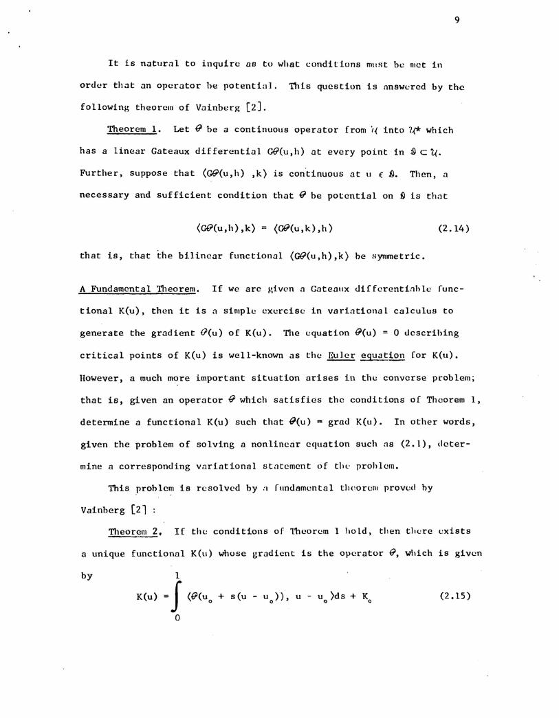
It is natural to inquire aB to what conditions must bc met in

order that an operator he potentia]. This question is answered by the

following theorem of Vainberg (2].

Theorem 1. Let @be a continuous operator from i{ into i(ok which

has a linear Gateaux differential GO(u,h) at every point in .i9 c?.{.

Further, suppose that (G@(u,h) ,k) is continuous at u (~. Then, a

necessary and sufficient condition that @be potential on il is that

(Gfil(u,h) ,k) = (G@(u,k),h)

that is, that the bilinear functional (G@(u,h),k) be symmetric.

(2.14 )

A Fundamental TIleorem. If we arc given n Gateaux di[ferentinhlc func-

tional K(u), then it is n simplc exercise in variational calculus to

generate the gradient O(u) of K(u). TIle equation @(u) = 0 dcscrihing

critical points of K(u) is well-known as the Euler equation [or K(ll).

However, a much more important situation arises in the converse problem;

that is, given an operator @ which satisfies the conditions of Theorem I,

determine a functional K(u) such that ~(u) IS grad K(u). In other words,

given the problem of solving a nonlinear equation such [IS (2.1), deter-

mine a corresponding variational statement of tIle prohlem.

This proh1em is resolved by ...fundamental theorem proved hy

Vainberg (21

Theorem 2. If the conditions of Theorcm 1 ho Id, tJlen there l~xists

a unique functional K(lI) whose gradient is the operator @, which is given

by

K(u)

1~Jo

(@(u + s(u - u », u - u )ds + Ko 0 0 0(2.15)

where Ko K(u ) and s is n real parameter.o

3 • SOM E EXAMPL ES

10

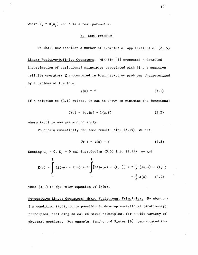
We shall now consider :l numher of examples of applications of (2.1:».

Linear Positive-Uefinite Operaton;. Mikh lin [51 presented n detailed

investigation of variationn 1 principles nssocintetl wi til l1ne:lr positive

definite operators S, encountered in houndnry-vn 1m' proh I ems charnctcrb:ed

by equations of the form

.£(u) = f (3.1)

If a solution to (3.1) exists, it can be shown to minimize the functional

J(u) = (u,j).J) - 2(u,f)

where (2.6) is now assumed to apply.

To obtain eS,sentinlly the s:une result \Ising (2.15), we Het

@(u) = S,(u) - f

Setting u = 0, K = 0 nnd introducing (3.3) into (2.15), we geto 0

(3.2)

(3.3)

_ 1- 2 J(u)

K(u)

1 1

= f (.I:(su) - f,u)ds = f[S(fu'U) - (f,u)]ds =

o 0

12 (j).J,u) - (f,u)

(3.4)

Thus (3.1) is tl~e Euler eq\lation of 2K(u).

Nonpositive Linear Operators, Mixed Variational Principles. TIy ahandon-

ing condition (2.6), it is possible to develop v[lriatiollal (stationary)

principles, including so-called mixed principles, for a wide varicty of

physical problems. For cxample, Sandhu and Plster (6] demonHtratcd the

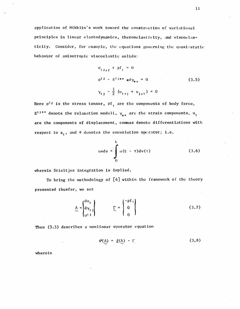
11

application of Mikhlin's work toward thc constrllction or variational

principles in linear elastouynomics, thermoelastil'ity, ;md viscoclns-

ticity. Consider, for example, the equations governing the qUllsi-static

behnvior of anisotropic viscoel;lstic solids:

lJ + pf = 01.l,J I

o (3.5)

1Y I J - "2 (u I '.1 + u J , \) = 0

Here alJ is the stress tensor, pf are tIle components of body force,1

E1Jmn denote the relaxation moduli, yare the strain components, u\mn

are the components of displacement, conunas denote differentiations with

respect to XI' and * denotcs the convolution 0JX.'r;ltor;i.e.

t

u,><Iv • f u(t - T)dv(T)

()

wherein Stieltjes integration is implied.

(J.6)

To bring the methodology of (6J within thc Cramework or the theory

presented thusfar, wc sct

IdU\ I.~ = dYI J

al J

(3.7)

Then (3.5) describcs a nonlinear operator equation

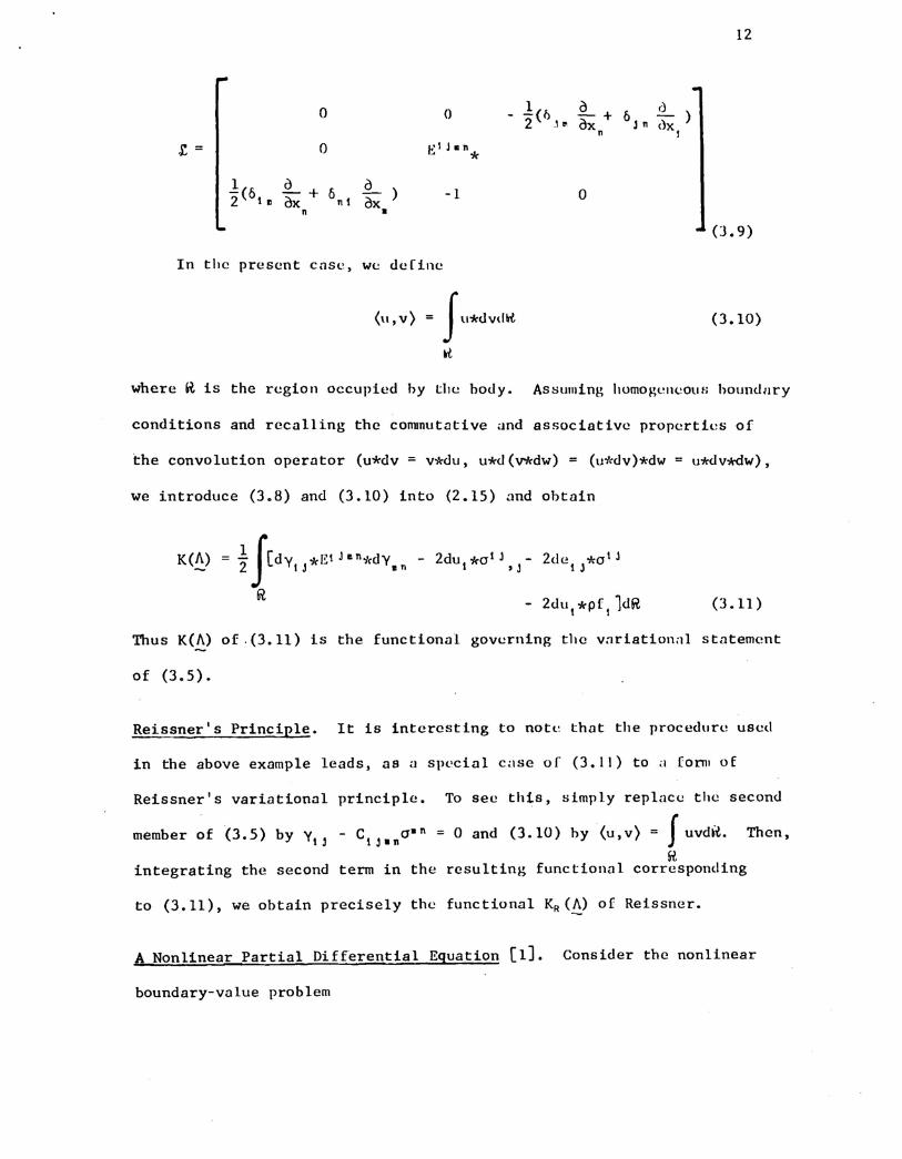
wherein

@(A) S.(A) - [' (J.8)

.£=

o

o

o

E1 hn*

-1 o

12

(3.9)

In the present case, we define

(u,v) (3.10)

where ~ is the region occupied hy the body. As~ulllinghomogl~IWOtW hounullry

conditions and recalling the conunut~tive and associative properties of

we introduce (3.8) and (3.10) into (2.15) and obtain

K(~) ~ J[dYlJ*!<1 Jo'*dY"

R (3.11)

Thus K(~) of. (3.11) is the function~l governing the v[lriation:ll statem(!t1t

of (3.5).

Reissner's Principle. It is interesting to note that dle procedure used

in the above example leads, as a special cnse of (3.11) to .:l forlllof

Reissner's variational principle. To sec this, simply replace the second

member of (3.5) by Yt3 - Ctj.no·n = 0 and (3.10) hy (u,v) = f uvd~. Then,

~integrating the second term in the resulting functional corresponding

to (3.11), we obtain precisely the functional KR(~) of Reissner.

A Nonlinear Partial Differential Equation (1]. Consider the nonlinear

boundary-value problem

13

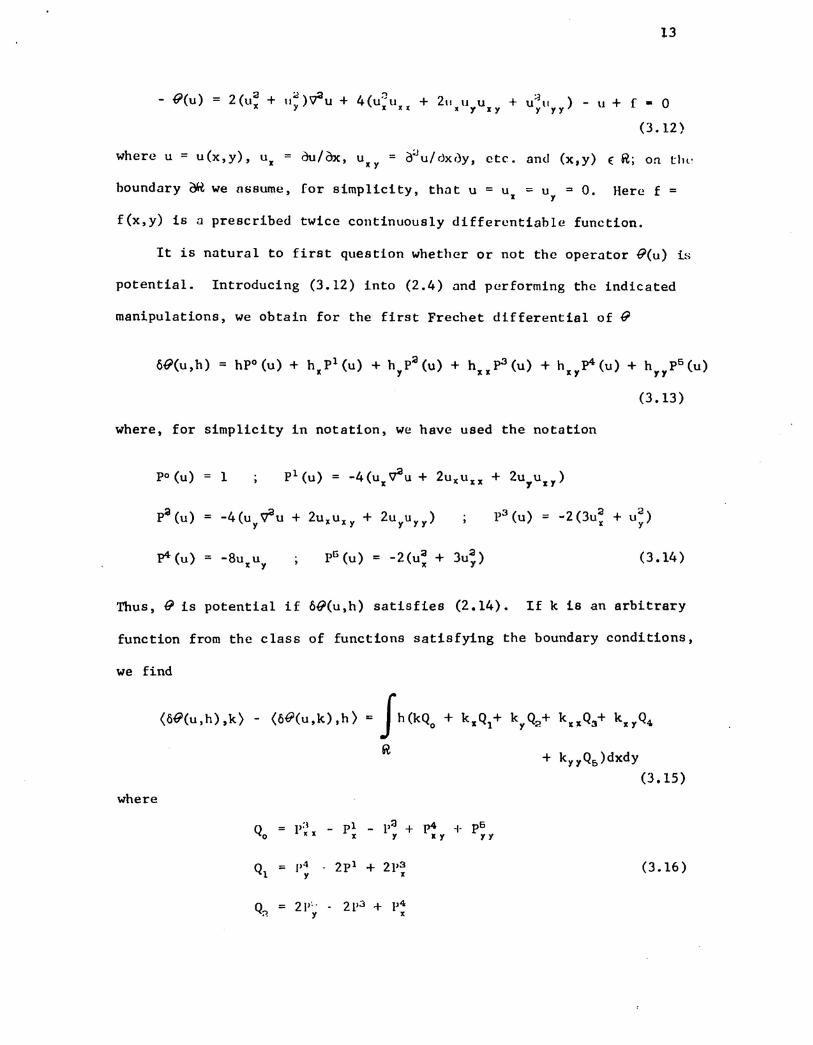
2 :J...2" :32 (ux + 11 )v-u + 4(u"u + 2\1U u + u 1I ) - U + f - 0y x xx x Y.Y 1 1Y

(3.12 )

~where u = u(x,y), u. = au/~, u = 0 u/dxoy, etc. and (x,y) € R; on thexy

houndary OR we assume, [or simplicity, that u = u = u = O. Here f• Y

f(x,y) is a prescribed twice continuously differcntiahle function.

It is natural to first question whether or not the operator @(u) is

potential. Introducing (3.12) into (2.4) and performing the indicated

manipulations, we obtain for the first Frechet differential of @

(3.13)

where, for simplicity in notation, we have used the notation

po (u) 1

p4 (u) = -Bux uy (3.14)

Thus, @ is potential if 6@(u,h) satisfies (2.l4). If k is an arbitrary

function from the class of functions satisfying the boundary conditions,

we find

(6@(u,h) ,k) -

where

(6@(u,k),h)' jh(kQ,

R + kyyQ,)dxdy(3.15)

Qo = 1'; x_ pl _ 1'2 + p4 -I- p5

x Y .y 11

Ql = 1'4 - 2pl + 21'3 (3.16 )1 x

Q = 21'~'. 2p3 + 1'4:'l Y x

14

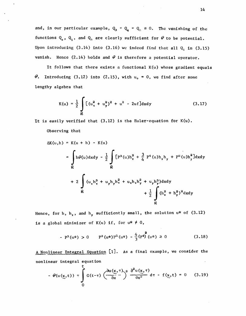
and, in our particular example, Qa = Q4 = Q!; = O. The vanishing of the

functions Qo' Ql' and Q~ are clearly sufficient for @ to be potential.

Upon introducing (3.14) into (3.16) we indeed find thot all Ql in (3.15)

vanish. Hence (2.14) holds and @ is therefore a potential operator.

It follows that there exists a functional K(u) whose gradient equals

@. Introducing (3.12) into (2.15), with Uo = 0, we find after some

lengthy algebra that

K(u) ~ !Ji [(u: + u;)· + u· - 2uf]dxdy

RIt is easily verified that (3.12) is the Euler-equation for K(u).

Observing that

~K(u,h) = K(u + h) - K(u)

(3.17)

- f h@(u)dxdy

R

+ 2 f (u h3x x

R

Hence, for h, hx' and hy sufficiently small, the solution u* of (3.12)

is a global minimizer of K(u) if, [or u* j 0,

- p3(u*) > 0~

p3 (u*)pG (u*) - !!. (p4) (u*) ~ 03

(3.18 )

~nlinear Integral Equation (l]. As a final example, we consider the

nonlinear integral equationt

f du(X, T) 2@(u(~, t» = G(t-,.) ( 0; - )

o

(3.19)

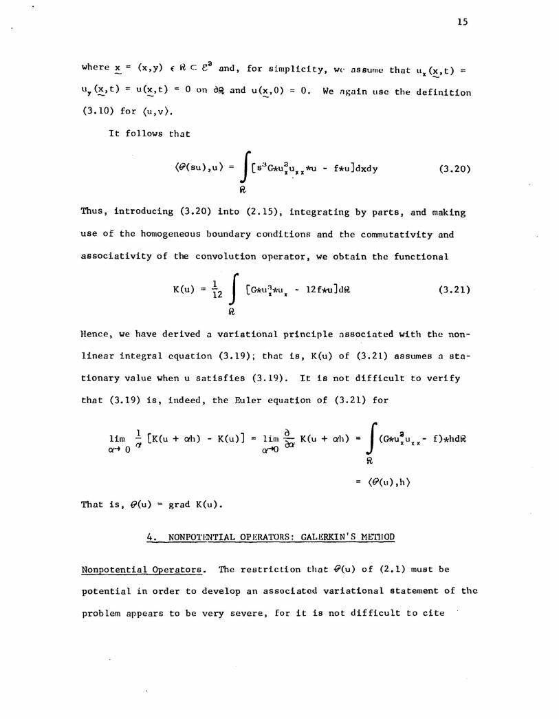
15

where x = (x,y) f.i c e:a and, for simplicity, We assuf1lethat ux(~,t) =

u (x,t) = u(x,t) = 0 on d~ and u(x,O) = O. We ngain use the definition'T _ _ _

(3.10) for (u,v).

It follows that

(@(su),u) J[S3~U:aU *u - f*u]dxdyx xx

~

(3.20)

Thus, introducing (3.20) into (2.15), integrating by parts, and making

use of the homogeneous boundary conditions and the commutativity and

associativity of the convolution operator, we obtain the functional

K(u) (3.21)

Hence, we have derived a variational principle ~ssociated with the non-

linear integral equation (3.19); that is, K(u) of (3.21) assumes Q sto-

tionary value when u satisfies (3.19). It is not difficult to verify

that (3.l9) is, indeed, the Euler equation of (3.2l) for

lim 1[K(u + ah) - K(u)]a--t 0 rt

(@(u),h)

That is, @(u) = grad K(u).

4. NONPOTENTIAL OPERATORS: GALERKIN'S ME'TII0D

NonpotentialOperators. The restriction that @(u) of (2.1) must be

potential in order to develop an associated variational statement of the

problem appears to be very severe, for it is not difficult to cite

l6

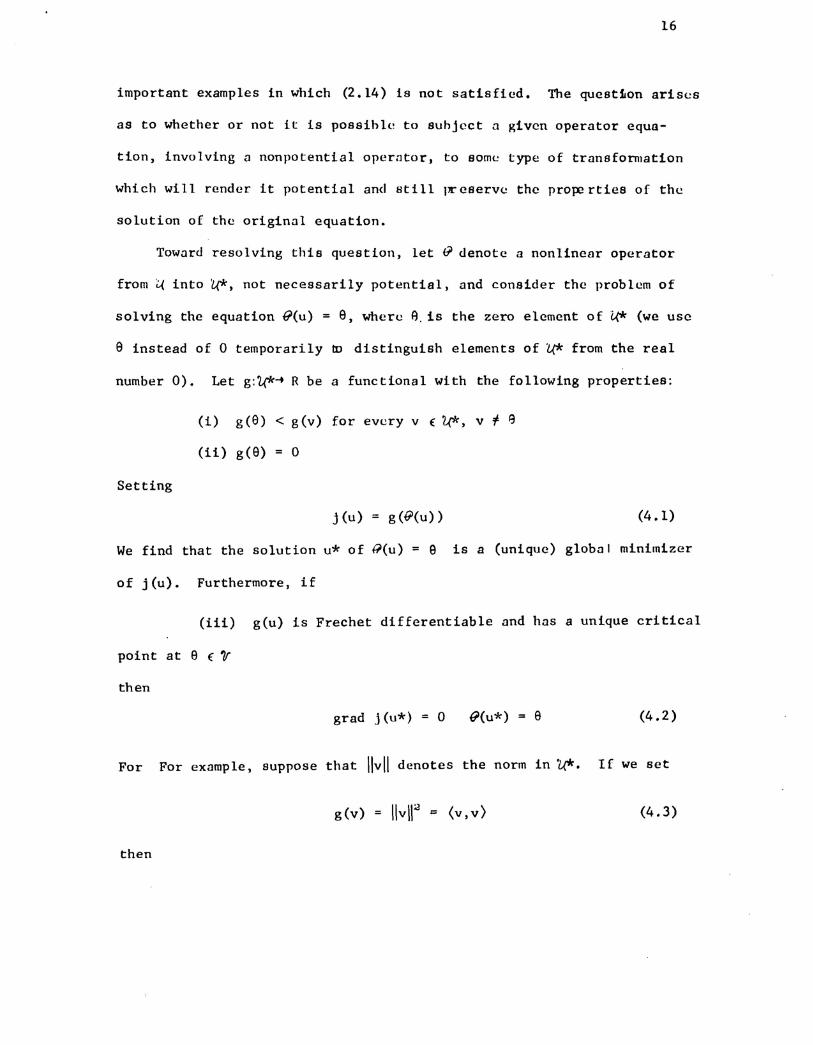
important examples in which (2.14) is not satisfied. The quest~on arises

as to whether or not it is possihle to suhjcct a given operator equa-

tion, involving a nonpotential operntor, to some type of transfornlation

which will render it potential and still preserve the pro}X:!rties of the

solution of the original equation.

Toward resolving this question, let @ denote a nonlinear operator

from ~ into U*, not necessarily potential, and consider the problem of

solving the equation @(u) = 8, where ~.is the zero element of U* (we usc

e instead of 0 temporarily w distinguish elements of U* from the real

number 0). Let g:U*~ R be a functional with the following properties:

(i) g(e) < g(v) for every v (4*, v i ~

(11) g(8) = 0

Setting

j(u) = g(@(u» (4.1)

We find that the solution u* of 9(u) = e is a (unique) global minimizer

of j(u). Furthermore, if

(iii) g(u) is Frechet differentiable and has a unique critical

point at 8 (~

then

grad j(u*) o @(u*) e (4.2)

For For example, suppose that I\vlldenotes the norm in 'Uk. If we set

then

g(v) IIvll2 = (v,v) (4.3)

17

j(u + ah) - j(u) = (@(u + ah), @(u + ah» - (@(u), @(u»

=llo@(u,ah)112+ 2(o@(u,O'h), O(u»

+ 2(w(u,ah), @(u» + (@(u + ah), w(u,ah»

and

lim l (j(u + ah) - j(u)] =arlO a

2 (O(u)(h), @(u» g (@(u» .@(u)(h)

(4.4)

Hence, if grad j(u*) = 0, g(e) = 0, which implies that v = e is the

critical point of g. Likewise, if O(u*) = e, then grad j(u*) = 0.

Obviously, the choice (4.3) leads to least-sguares approximations.

Still other choices are possible. For example, if £ is a positive-

definite, symmetric, linear operator on U*,the procedure leading to (4.4),

with j(u) (£V,v),v = @(u) yields

(grad j(u),h) = 2(~(@(u», @(u)(h» (4.5)

Since h can assumedly be taken from outside the null space of the linear

operator ~(u), vanishing of (4.5) implies that ~(@(u*» = 0. But since

~ is positive definite, the unique solution of ~(@(u*» = 0 is @(u*) = e,

which is the solution of the original problem. Finally, we remark that

operating on both sides of certain nonpotential linear equations with

the convolution operator * of (3.6) is often sufficient to transform

them into potential operators •

.Gelerkinls Method. It is interesting to note that the idea of potentiol

operators can be used to motivate the approximate solution of (2.1) by

Galerkin's method. Let @ be a potential operator defined on a set ~ of

a Hilbert space U and let U denote a G-dimensional subspace of ~ spanned

by a set of G linearly independent functions CPt(~), cp~(~), ••. '% (~) (L(.

18

We wish to determine coefficients aa so that the function

au = a ~ (x) (4.6)a-

represents an approximate solution to (2.1) in U. Since @ is a potential

operator, there exists a functional K(u) such that grad K(u) = @(u);

indeed, if u* is the solution of (2.1), grad K(u*) = @(u*) = O. In

view of (2.9), this means that

(@(u*),h) = 0 (4.7)

In other words, @(u*) = 0 by virtue of the fact that it is orthogonal

to every h in a set ~o assumed to be dense in U.

Galerkin's method amounts to forcing @(u) to satisfy (4.7) in U.

If h is an arbitrary element of U, we set

(4.8)

Band since (4.8) must hold for arbitrary coefficients h , we have

(4.9)

Equations (4.9) represent G independent (generally nonlinear) equations

ain a which, when solved, determine the approximate solution (4.6). We

also observe that (4.9) represents the requirement that the residual

be orthogonal to «. In fact, (4.9) must be satisfied if u of (4.6) is

to be the "best" approximation of u in U. To prove this assertion,o

assume the contrary; i.e. (-ro,h) a f 0, and, without loss in gener-

ality, set Ilhll= 1. Then, if r = ro + ah E '£.{, consider

(@(u*) - ro - ah, @(u*) - ro - ah)

19

- ro,h) + ai

Since @(u*) = 0, (h,@(u*) - r )o (h, - r ) = a ando

Consequently, the measure \I@(u*) - @(~)II is a minimum when a = O. Then

r = ro and (ro,h) = 0, as indicated in (4.9).

5. FINITE ELEMENT APPROXIMATIONS

We are now ready to investigate the theory of finite element approxi-

mations of nonlinear operators. In particular, we are interested in the

problems of interpolation using finite elements, error estimates, cri-

teria for the selection of local interpolation functions, and convergence.

To keep the scope within reasonable bounds, we restrict our discussion

of these last two subjects to the case in which critical points of the

functional K(u) are at least local minimizers of K(u).

General Finite Element Models. Following (4], we shall first reproduce

certain general properties of finite-element models of a real-valued

function U(x) defined on a region ~ of ek, with x ~ (Xl'Xi, ••• ,xk).

The following procedure is used:

To construct a finite element model of U(~), we partition R into

E subregions fl,f2, ••• fr (finite elements) connected continuously to-

6gether along interelement boundaries. While X denote global nodal

points in the "connected model" R of R, locally we denote nodal points

20

in clement r" by~, N = l,2, •••,N.; N" being the number of nodal points

of r. The decomposition of R into elements is then implied by"

(5.1)

e

where the Boolean matrix ~ = 1 if node N of r. is coincident with node

6 in the connected model and ~ = 0 if otherwise. Here and henceforth,

repeated nodal indices 6(N) are summed from 1 to G(N). Also, for slm-"

plicity, we assume that the local and global coordinate systems x ,x-" -

coincide and we affix an element label (e) on various local quantities

only when their local character is of special importance or is not cle~

in the context.

Let u (x ) denote the restriction of U(x) to r and let uN, uN l'• ....Jl _. e e,

•••,uN,! t denote the values of u (x) and its partial derivativese i"'r e_

up to order r at node N or

of u (x) is of the forme _

r •"

TIle local finite-element representation

(5.2)

where N is summed from 1 to N. and the interpolation functions W~(~),...,1 1 ••• 1

WN r (~(il ~ ia ~ ... ~ ir = 1,2,•.•,k) have the following proper-

ties:

(i)

r -I s

r = s

(5.3)

(ii) If l is a characteristic length of r , there exist boundede •

dimensionless functions ~~(S),where S = Xt/te, such that_ t

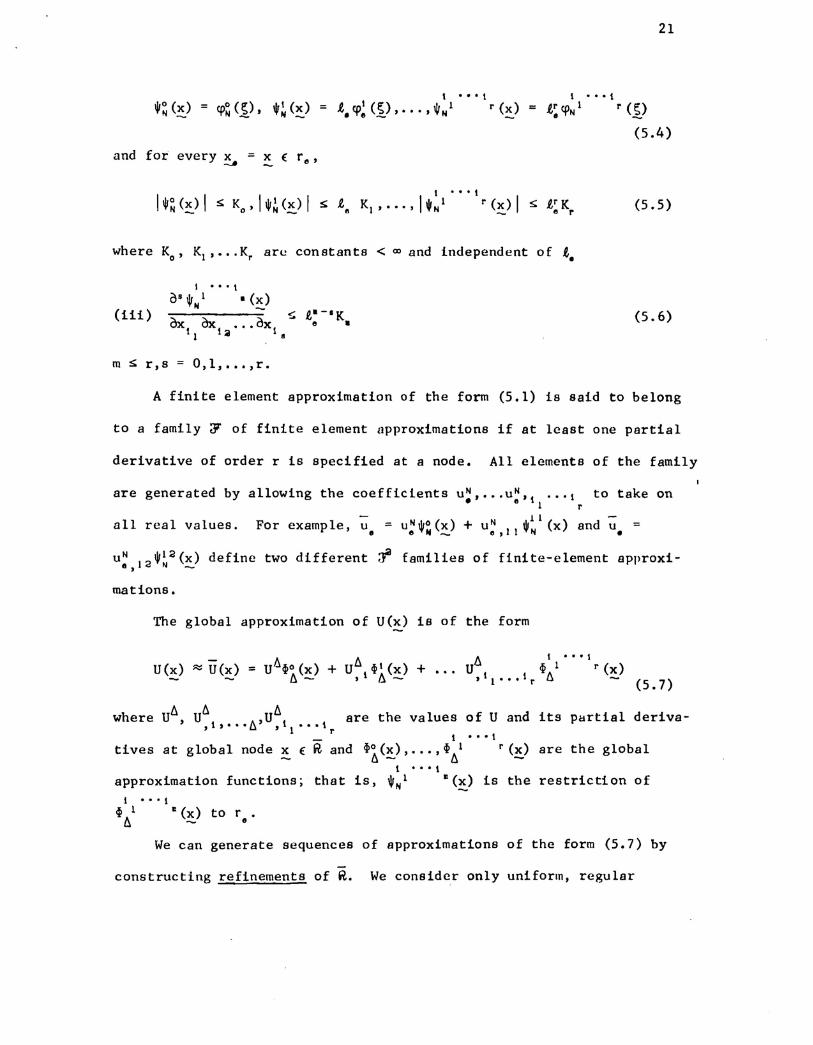
and for every x = x ( f",-...II _

1 -. - 1l.tt>; (~), ••• ,WN1 r (X)

21

1 ---It~tt>N1 r (.9

(5.4)

I ••• t

IW~(~)I S; Ko.lw~(~)1 S; t" K1, ... ,I.N1 r(~)1 s; .e:Kr

where Ko' KI,••.Kr are constants < 00 and independent of t.

(5.5)

(iii) (5.6)

m S; r,s = O,l, ••• ,r.

A finite element approximation of the form (5.l) is said to belong

to a family ~ of finite element approximations if at least one partial

derivative of order r is specified at a node. All elements of the family

are generated by

all real values.

allowing the coefficients uN, ••.uH" ••• \ to take on• ... 1 r

11 -For example, u = uNWON(X) + UN IIWu (x) and u =e e _ e, '"1 •

U(x) ~ U(x)

uH I",W12(x) define two different ;f families of finite-element approxi-tt) <0 N _

mations.

The global approximation of U(x) is of the form

/). 6 6 t ... \= U ~~(x) + U I~~(X) + ... U t \ ~A1 r(x)

u - "~ - , 1'" r U - (5.7)

~ 6 ~where U , U,t""6,U,1 .••1 are the values of U and its partial deriva-1 r_ 1 ···1

tives at global node ~ (6t. and ~6(~), ••• ,~~1 r(~) are the global1. ••• 1

approximation functions; that is, .,/ ..(~) is the restriction of\ ... \

~ 1 .. (x) to r •~ _ "We can generate sequences of approximations of the form (5.7) by

constructing refinements of R. We consider only uniform, regular

22

refinements; i.e. refinements in which the same types of elements and

interpolation functions defined on R are used for ~I and every node and

interelement boundary in R is a node and interelement boundary in RI•

The diameter 0 of an element r is the maximum distance between two• e

points xA, Y (r (0 = max !Ix - v II), and the mesh 0 of a model bt is__ :..J/J e e -JI 0 -

the maximum diameter of all elements in R(o - max (61,0 ""'Or)' Oh-;:)

viously, for a sequence of refinements ~] we require that the meshes

or ....a as r ....<Xl.

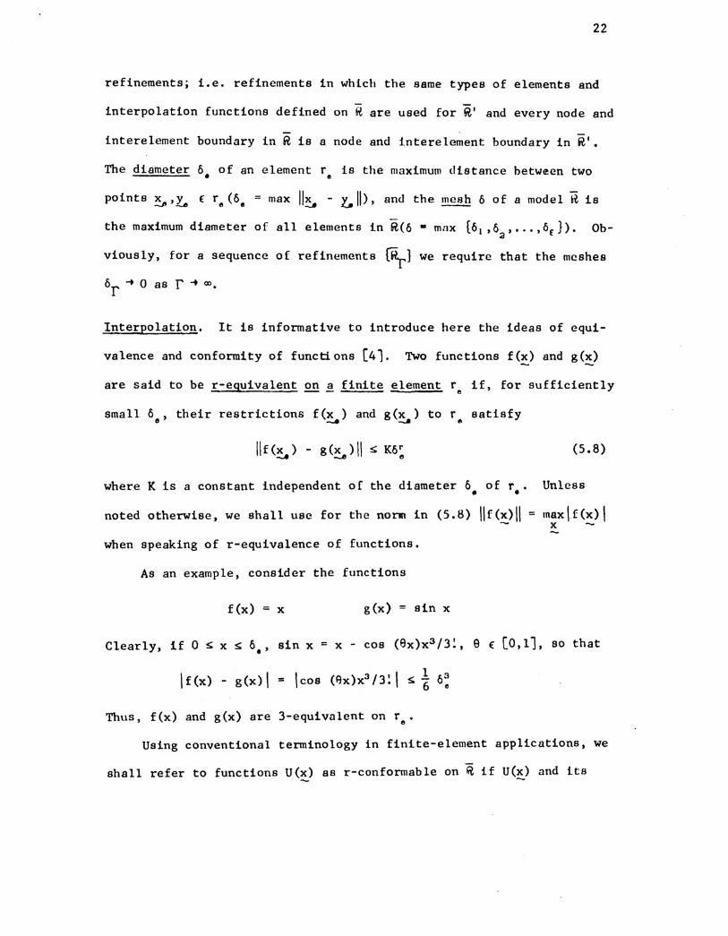
Interpolation. It is informative to introduce here the ideas of equi-

valence and conformity of functions (41. Two functions f(x) and g(~)

are said to be r-eguivalent £g ~ finite element re if, for sufficiently

small 0 , their restrictions f(x ) and g(x ) to r satisfye ....... -..A II

where K is a constant independent of the diameter 0 of r. Unless• •noted otherwise, we shall use for the norm in (5.B) Ilf(~)1Iwhen speaking of r-equivalence of functions.

As an example, consider the functions

= max \f(x) Ix -

f(x) x g(x) = sin x

Clearly, if 0 ~ x ~ 6., sin x = x - cos (ex)x3/3~, e ( [0,11, so that

\f(x)

Thus, f(x) and g(x) are 3-equivalent on r .e

Using conventional terminology in finite-element applications, we

shall refer to functions U(x) as r-conformable on ~ if U(~) and its

23

partial derivatives up to order r are continuous throughout ~; that is,

U (x) is r-conformab Ie if U (~) € Cr (It) •

We have now set the stage for investigating the question of inter-

polation, or approximation, of a givcn function U(x) by a finite element~

model U(x). We obtain the properties of such approximations through the

following theorem, which represents a generalization and revision of the

work of Arantes e Oliveira (3].

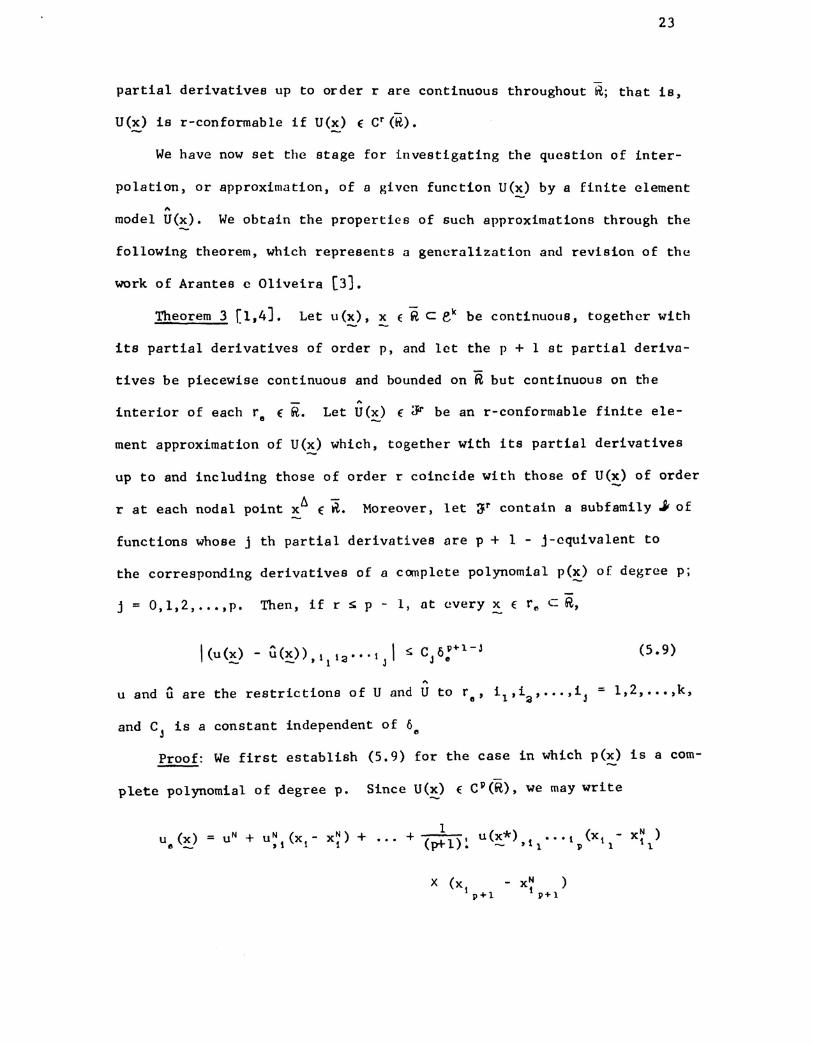
Theorem 3 [1,4]. Let u (x), x ERe ek be continuous, together with

its partial derivatives of order p, and lct the p + 1 st partial deriva-

tives be piecewise continuous and bounded on ~ but continuous on the

"interior of each f € R. Let U(x) E ~ be an r-conformable finite ele-e _

ment approximation of U(~) which, together with its partial derivatives

up to and including those of order r coincide with those of U(~) of order

tJ -r at each nodal point ~ €~. Moreover, let ar contain a subfamily ~ of

functions whose j th partial derivatives nre p + 1 - j-cquivalent to

the corresponding derivatives of a complete polynomial p(~) of degree p;

j = 0,1,2, .••,p. Then, if r ~ p - 1, at every x € fll C R,

I(u(x) - u(x» 1 1""'\ 1$ CJoP+1.-J- -, 1" J ..

u and u are the restrictions of U and U to fe' i1,ia,···,ij

(5.9)

1,2, .•• ,k,

and CJ

is a constant independent of 6e

Proof: We first establish (5.9) for the case in which p(x) is a com-- -plete polynomial of degree p. Since U(~) E cP (R), we may write

u (x)Il _1

UN + uN1(xl- xN) + ... + (P+l)' u(x*) t ••• \ (XI - X

N1 )

, I • -'1 P 1. 1.

24

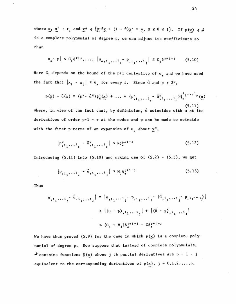
where x, XN € rand x* € (y:ex + (1 - e)xN a y, 0 S e S I}. If p(x) € ~__ e _ __ _ _ _

is a complete polynomial of degree p, we can adjust its coefficients so

that

P 1 ••• 1.1' 1

(5.10)

Here Cj depends on the hound of the p+l derivative of ue

and we hove used

the fact that IX1 - Xl I s; 6" for every 1. Since u and p ( ;P,

(5.11)where, in view of the fact that, by definition, u coincides with u at its

derivatives of order p-l = r at the nodes and p can be made to coincide

with the first p terms of an expansion of u about xN,e _

(s.l2)

Introducing (5.11) into (5.10) and making use of (5.2) - (5.5), we get

Thus

Ip 1 - u I S; M t. p+ t - J,11", .I ,1t···1j jUe

(5.13)

= \u - p - (u - p }I'1 ••• 1 ,1 ••• 1.1 ,1 ••• 1 ,11'''1

1 .I 1 1.\

S (C + M )6P+1-.\ = C6P+1-.\.\ .\. "

We have thus proved (5.9) for the case in which p(~) is a complete poly-

nomial of degree p. Now suppose that instead of complete polynomials,

.it contains functions ~(~) whose j th partial derivatives are p + 1 - j

equivalent to the corresponding derivatives of p(x), j = 0,1,2 ••••,p.

25

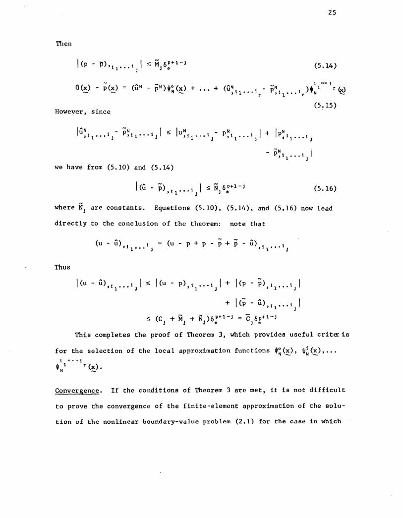
Then

(5.14)

However, since

+ ... +

-N I- P,11"·IJ

we have from (5.10) and (5.14)

I(u-p) IIS:NOP+I-J,11'" J J e

(5.16)

where Nj are constants. Equations (5.10), (5.14), and (5.16) now lead

directly to the conc lusion of the theorem: note that

(u - u) I C (u - p + P - P + P,11". j

Thus

I(u - U),t ... 1 I:s: I(u - P),1 .. ot 1+ I(p - P),ll ... l I1 J 1 J J

+ I(p - U),11 •• .1j

Is: (C + M + N )6P+1-j = C 6p+l-j

J j J II j II

This completes the proof of Theorem 3, which provides useful crit~ia

for the selection of the local approximation functions .~(~), .~(~), •••1 ••• 1

+N 1 r (~).

Convergence. If the conditions of Theorem 3 arc met, it is not difficult

to prove the convergence of the finite-element approximation of the solu-

tion of the nonlinear boundary-value problem (2.1) for the case in which

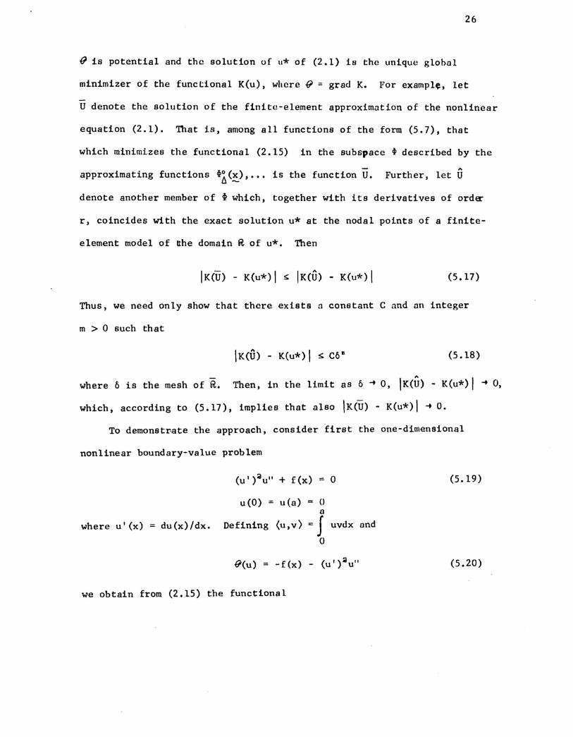
26

Q is potential and the solution of u* of (2.1) is the unique global

minimizer of the functional K(u), where @ = grad K. For example, let

U denote the solution of the finite-element approximation of the nonlinear

equation (2.1). That is, among all functions of the form (5.7), that

which minimizes the functional (2.15) in the subspace t described by the

approximating functions ~6(~)'." is the function U. Further, let Udenote another member of ~ which, together with its derivatives of ord~

r, coincides with the exact solution u* at the nodal points of a finite-

element model of tthedomain R of u*. Then

(5.17)

Thus, we need only show that there exists n constant C and an integer

m > 0 such that

\K(U) - K(u*) \ s C6~ (5.18)

where 6 is the mesh of R. Then, in the limit as 6 ~ 0, lK(U) - K(u*) I ~ 0,

which, according to (S.l7), implies that also IK(U) - K(u*) I ~ o.

To demonstr-ate the approach, consider first the one-dimensional

nonlinear boundary-value problem

where u I (x)

u(O) :;u(a) == 0a

du(x)/dx. Defining (u,v) == J uvdx and

o

@(u) = -f(x) - (u' )Olu"

(5.19)

(5.20)

we obtain from (2.15) the functional

a

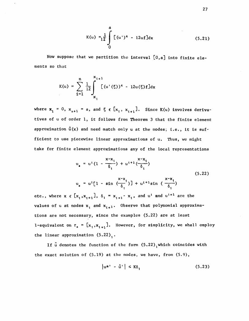
K(u) -If f [(u')4 - I2uf]dx

°

27

(5.21)

Now supposc that we partition the interval (O,a] into finite ele-

ments so that

n Xl+l

K(u) = L i2f (u I (S»4 - 12u (S)f]dx

i=lXl

where xl = 0, Xn+l = a, and S € [Xl' xl+1J. Since K(u) involves deriva-

tives of u of order 1, it follows from Theorem 3 that the finite element

approximation u(x) and need match only u at the nodes; i.e., it is suf-

ficient to use piecewise linear approximations of u. Thus, we might

take for finite element approximations any of the locol reprcsentations

(5.22)

uo

X-Xl X-Xlsin (--- )J + ul+1sin (----)

01 6t

etc., where X E (Xl,xl+1J, 01 = Xl+1- xt' and u1 and ul+1 are the

values of u at nodes Xl and xl+1' Observe that polynomial approxima-

tions are not necessary, since the examplcs (5.22) are at least

I-equivalent on To = [xt,xl+1

]. However, for simplicity, we shall employ

the linear approximation (5.22)1'

If ~ denotes the function of the form (5.22)lwhich coincides with

the exact solution of (5.19) at the nodes, we have, from (5.9),

(5.23)

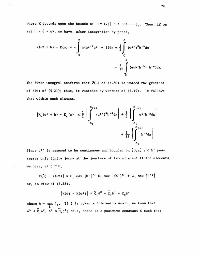
28

where K depends upon the bounds of IU*"(X) I but not on 0t' Thus, if We

set h = u - u*, wc havc, after integration hy parts,

a

K(u* + h) - K(u) • - f h(u*,au*" +

o

a

f)dx + 1J (u*' )ah ,adx

oa

+ 1-J (4u*'h'3+ h'4)dx12

o

The first integral confirms that @(u) of (5.20) is indeed the gradient

of K(u) of (5.21); thus, it vanishes by virtues of (5.19). It follows

that within each elemcnt,

1+ 12

Since u*' is assumed to be continuous and bounded on [O,a] and h' pos-

sesses only finite jumps at the juncture of two adjacent finite elements,

we have, as 0 ~ 0,

\K(u) - K(u*) I s; C1 max Ih'10'1+ C:, max I (h')3\ + C~ max Ih "I. I

or, in view of (5.23),

where 6 = max 6t• If 6 is taken sufficiently small, we know thati

&3 s; C~&2, &4 s; C~64; thus, there is a positive constant C such that

29

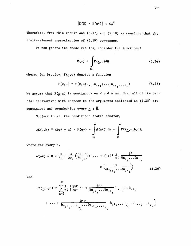
Therefore, from this result and (5.17) and (5.18) we conclude that the

finite-element approximation of (5.19) converges.

To now generalize these results, consider the functional

K(u) ~ .fF(~'U)dR

~

where, for brevity, F(~,u) denotes a function

F (x, u) = F (x, u; U, I ; u, I J ; ••• ,u, 11' •• I p)

(5.24 )

(S. 2S)

We assume that F(~,u) is continuous on ~ and ~ nnd that all of its par-

tial derivatives with respect to the arguments indicated in (5.25) are

continuous and bounded' for every ~ ( R..

Subject to all the conditions stated thusfar,

6K(u,h) " K(u* + h) - K(u*) • f@(U*)hdR + JF*(~,u,h)dR

R ~

where,for every h,

and

(5.26 )

F* (::.'u,h) = ~ 1 ronF hn + anFL n~ Loon aU,1 ...au>!n=2 1 n

h I ••• h 1, 1 'n

+ ... anF+ '::L.. 1 ••• 00,1 ••• lpuut ••• ", n

, 1'1 n

hl· .. h 1 1 J,tl••• P , n··· P ~1 n

30

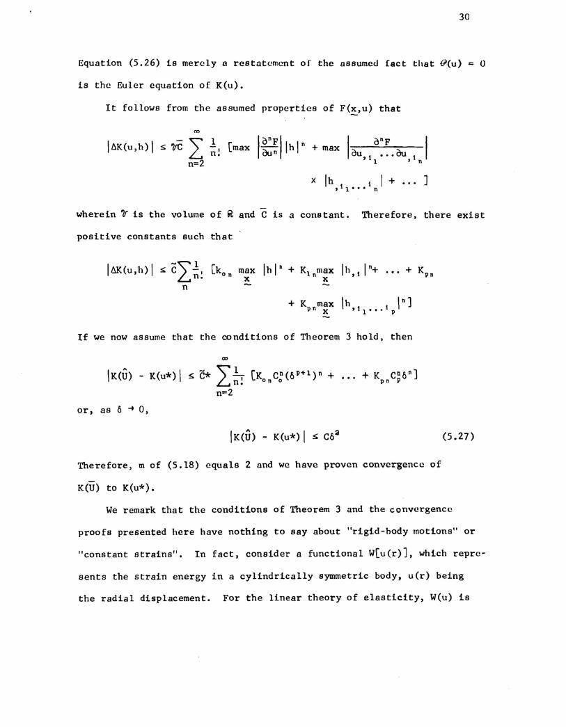
Equation (5.26) is merely a restatement of the assumed fact that tfl(u):::0

is the Euler equation of K(u).

It follows from the assumed properties of F(~,u) that

m

- ~ 1 lonFI16K(u,h) I s ?IC L ~~(max aun IhI n + max

n=2

wherein ~ is the volume of ~ and C is a constant. Therefore, there exist

positive constants such that

-II16K(u,h)lsC -,(konn.n

maxx

Ih I n + Kl maxn X

If we now assume that the conditions of TIleorem 3 hold, then

\K<ih - K(u*) I s c* ~.!...... (K CD(6P+1)n + ... + K CDon]Ln~ On 0 pn P

n=2

or, as 0 ... 0,

(5.27)

Therefore, m of (5.18) equals 2 and we have proven convergence of

K(U) to K(u*).

We remark that the conditions of Theorem 3 and the convergence

proofs presented here have nothing to say about "rigid-body motions" or

"constant strains". In fact. consider a functional W(u(r)], which repre-

sents the strain energy in a cylindrically symmetric body, u(r) being

the radial displacement. For the linear theory of elasticity, W(u) is

31

a quadratic form in u and du/dr and the circumferential strain Yee= u/~

However, according to Theorem 3, a perfectly acceptable approximation octhe displacement ue in an element r f Crt' rt+1], 0 ~ a ~ 2n, is u =

a + br, a and b heing constants. Consequently, Yae = (a + br)/r so that

arbitrary a and b cannot produce a rigid motion nor is Yae constant

throughout an element.

Finite-Element Models. In concluding this lecture, we point to properties

of the discrete analogues of (2.9) and (4.7). In local finite-element

approximations, functions are approximated by elements of a certain class

which are generally representable in the form u = uN(t)W (x) (or, moreN _

generally, of the form (5.2». Thus, on a discrete scale, K(u) becomes

a functional of only the nodal values UN and/or nodal values of the deri-

vat! veS and the hilinear functiona 1 (2.5) aSsumcs a form which depends

upon the definition of (\I,v)in the continuum solution. For example, if

(u,v), • JUVdRR

or (u,v>" • JU*VdR~

Thus, if @N(u) denotes thc local finite element

(~;) = C uNVM, 1 NM

= !WN.Mdre'r

IInonlinear equation @(u) = 0, (4.7) leads to relations of themodel of a

form

(5.28)

etc., so that in any case @N(~) = 0 due to the arbitrariness of the

nodal values hN•

32

For example, in constructing a finite-element approximation of

(3.12), we may use as local representations

(5.29)

where aN and bNa are constants depending only on the geometry of a

triangular element of area Be and Xl = x, x2 = y, a = 1,2, N = 1,2,3.

The functional (3.17) becomes

where

AN''' ~ a.b,,,b,,,b, ab,a BNN ~ f .,',dxdy

r~

Thus, minimizing Ke(u) among all functions of the form (5.24) and using

(5.28), we obtain the system of cubic equations,

Global forms are obtained by connected elements together in the usual

fashion.

Likewise, in the case of the nonlinear integral equation (3.19),

use of (3.21) and (5.29) leads to

(5.30)where

Jlf(~.t)~,(X)dXdY

r e

33

Since hN(t) and their histories are arbitrary, the term in brackets in

(5.30) must vanish, and we obtain as a discrete model of (3.21) a

system of nonlinear integral equations in uN(t).

6. REFERENCES

1. Oden, J. T., "Finite Element Models of Nonlinear Operator Equations",Proceedings of the Third Conference on Matrix Methods in StructuralMechanics, Wright-Patterson Air Force Base, Ohio, 1971.

2. Vainberg, M. M., Variational Methods for the Study of NonlinearOperators, (TranSlated from the 1956 Russian edition by A. Feinstein),Holden-Day, San Frnncisco, 1964.

3. Arantes e Oliveira, E. R., "Theoretical Foundations of the FiniteElement Method", International Journal of Solids and Structures,Vol. 4, pp. 929-952, 1968.

4. Oden, J. T., Finite Elements of Nonlinear Continua, McGraw-Hill,New York, 1971.

5•• Mikhlin, S. G., Variational Principles in Mathematical Physics,(Translated from the 1957 Russian edition by T. Boddington)Pergamon Press, Oxford, 1964.

6. Sandhu, R. S. and Pister,K. S., "A Variational Principle for LinearCoupied Field Prob lems in Continuum Mechanic s", InternationalJournal of Engineering Sciences, Vol. 8, pp. 989-999, 1970.