A FINITE ELEMENT FORMULATION FOR NONLINEAR 3DCONTACT PROBLEMS

Federico J. Cavalieri, Alberto Cardona, Víctor D. Fachinotti and José Risso

Centro Internacional de Métodos Computacionales en Ingeniería(CIMEC-INTEC). CONICET - Universidad Nacional del Litoral

Güemes 3450, (3000) Santa Fe, Argentina, acardona@intec.unl.edu.ar http://www.cimec.org.ar

Keywords: Contact, Rockafellar Lagrangian, finite elements, penalty,friction

Abstract. A finite element formulation to deal with friction contact between an elastic body and arigid obstacle is presented. Contact between flexible solids or between a flexible and a rigid solid is de-fined using a non-penetration condition which is based on a representation of the interacting deformingsurfaces. A large number of contact algorithms based on the imposition of inequality constraints weredeveloped in the past to represent the non penetration condition. We can mention penalty methods, La-grange multiplier methods, augmented Lagrangian methods and many others. In this work, we developedan augmented Lagrangian method using a slack variable, which incorporates a modified Rockafellar La-grangian to solve non linear contact mechanics problems. The use of this method avoids the utilizationof the well known Hertz-Signorini-Moreau conditions in contact mechanics problems (coincident withKuhn-Tucker complementary conditions in optimization theory). The contact detection strategy makesuse of a node-surface algorithm. Examples are provided to demonstrate the robustness and accuracyof the proposed algorithm. The contact element we present can be used with typical linear 3-D ele-ments. The program was written in C++ under the OOFELIE environment. Finally, we present severalapplications of validation.

1 INTRODUCTION

In this work we present numerical solutions of contact problems in non linear elasticity.Such problems arise in many mechanical engineering applications and several works dedicatedto numerical solution of contact problems have been published in the literature. Applicationsof contact mechanics in mechanical engineering include the design of gears, wear in compo-nents, metal forming processes like sheet metal or bulk forming, etc. Several papers presentnew advances and techniques for solving contact problems, including friction, plasticity, wear,surface fatigue wear or large deformation of 3D deformable solids. However there is not yet acompletely robust algorithm suitable for different applications.

The penalty method is today widely used in optimization techniques. This is because thedisplacement being the only primal variables that enter in the formulation, this method is easierto program than others. However, it is extremely dependent on mesh size, it allows some pen-etration between contacting bodies and, as it is well known, the user must choose the correctvalue of a parameter (the “penalty”) in a rather arbitrary way to get good results. Therefore,many tests have to be carried out to verify convergence. Also, algorithms based on these meth-ods generate ill-conditioned matrices and the convergence is very slow when the mesh gets fine(it is however possible to avoid ill-conditioning).

The methods of multipliers are very popular in contact finite element analysis. Particularly,the augmented Lagrangian technique, well known in optimization theory, overcomes the prob-lem of ill-conditioning of penalty methods. Both augmented Lagrangian and penalty methodsrequire a penalty parameter, but in the augmented Lagrangian method the role of the penaltyparameter is only to improve the convergence rate. It is also clear that in penalty methods,increasing the penalty factor to infinity would yield the exact solution, but in computationalapplications it is not possible to use very large penalty factors because of ill-conditioning.

In fact, it makes sense to adopt multiplier Lagrange methods. The Lagrange multiplier meth-ods fulfil the contact constraints exactly by introducing additional variables; for this reason theLagrange multipliers generate an increment in matrix size. A combination of the penalty methodand the Lagrange multipliers technique leads to the so-called augmented Lagrangian methods,which try to combine the characteristics of both Bertsekas (1984). The Uzawa scheme relatedto the augmented Lagrangian method can be applied to improve the solution.

We present here a finite element method to solve contact problems through the utilization of amodified augmented Lagrangian. This technique is known as modified Rockafellar Lagrangianstrategy. We use a slack variable to handle the inequality of the constrained problem. The paperis organized in the following way. First we present the mathematical formulation of contactfrictionless problem giving a solution for the equivalent variational problem. Then, we discussabout the advantages of slack variables. We give general considerations about the modifiedRockafellar Lagrangian method. Section 5 is dedicated to the study of contact detection strategy.Section 6 contains general considerations about the friction problem. Finally, section 7 providesa numerical application.

2 CONTACT PROBLEM DESCRIPTION AND VARIATIONAL FORMULATION

In this section we will review the contact problem when an elastic body comes into contactwith a rigid foundation, and the notation used throughout this work (Belhachmi and Ben Bel-gacem, 2001).

We will begin with a description of the basic equations of elasticity and then, since we willapply the finite element method to solve the boundary value problem, we will present a weak

formulation of the contact problem.The equilibrium equation in elasticity is:

Div σ(u) + b = 0 in Ω, (1)

where σ is the stress tensor and b is the body force. The strain tensor ε(u) is:

ε(u) =1

2[ Grad (u) + Grad T(u) + Grad T(u) · Grad (u)] (2)

The gradient and divergence operators are evaluated at initial configuration (Ogden, 1984).The relation between the stress and the strain is established via the classical Hooke law:

σ(u) = C : ε(u) (3)

where C is the constitutive fourth-order tensor, symmetric and elliptic.

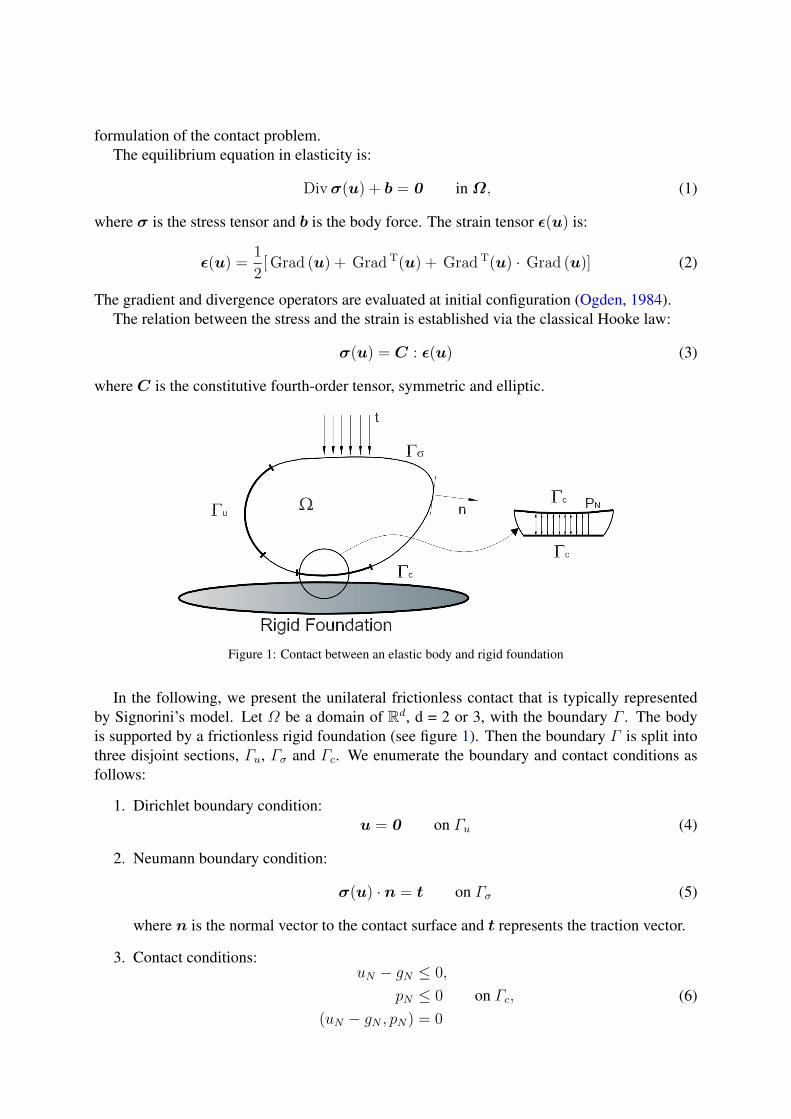
Figure 1: Contact between an elastic body and rigid foundation

In the following, we present the unilateral frictionless contact that is typically representedby Signorini’s model. Let Ω be a domain of Rd, d = 2 or 3, with the boundary Γ . The bodyis supported by a frictionless rigid foundation (see figure 1). Then the boundary Γ is split intothree disjoint sections, Γu, Γσ and Γc. We enumerate the boundary and contact conditions asfollows:

1. Dirichlet boundary condition:u = 0 on Γu (4)

2. Neumann boundary condition:

σ(u) · n = t on Γσ (5)

where n is the normal vector to the contact surface and t represents the traction vector.

3. Contact conditions:uN − gN ≤ 0,

pN ≤ 0 on Γc,

(uN − gN , pN) = 0

(6)

In this work we will present an algorithm for normal contact (using a modified Rockafellaraugmented Lagrangian technique), so we will only work with the normal component of thetraction vector defined by pN = t · n, the normal distance uN , and the normal initial gap gN .

The body is fixed on Γu, the contact surface is Γc and the surface traction pressure is appliedon Γσ.

Signorinis’s problem consists in: Find a displacement u ∈ Ω, which is solution of thefollowing system of equations:

Div [σ(u)] + b = 0 in Ω,

u = 0 on Γu,

σ(u) · n = t on Γσ,

uN − gN ≤ 0,

pN ≤ 0 on Γc,

(uN − gN , pN) = 0.

(7)

For a finite element solution we need the variational formulation of Signorini’s problem. Weintroduce a Hilbert space V such that:

V =v ∈ H1(Ω)d : v = 0

on Γu (8)

and a set admissible displacements K defined of the following way:

K = v ∈ V : vN − gN ≤ 0, on Γc with vN = v · n (9)

Starting from equilibrium equation, multiplying it by an arbitrary function v ∈ V and by usingGreen’s formula we obtain:∫

Ω

σ(u) : ε(v) dx =

∫Ω

b · v dx +

∫Γσ

t · v ds +

∫Γc

pNvN ds (10)

Let us define a bilinear form a and a linear form L in the form:

a(u, v) =

∫Ω

σ(u) : ε(v) dx ∀u, v ∈ V,

L(v) =

∫Ω

b · v dx +

∫Γσ

t · v ds +

∫Γc

pNvN ds ∀v ∈ V.(11)

Then, equation (10) may be rewritten as:

a(u, v) = L(v) ∀v ∈ V. (12)

Is not difficult to show that a(u, v) is symmetric, continuous and V -elliptic Johnson (1995).It is important to note that the term Γu is not included in (11) because it satisfies the Dirichletcondition. Now suppose first that u is the solution to V , v ∈ V and a set w = v − u such thatw ∈ V . The Signorinis’s problem defined by (7) is reformulated as:

∫Ω

σ(u) : ε(v−u) dx =

∫Ω

b · (v−u) dx +

∫Γσ

t · (v−u) ds +

∫Γc

pN(vN − uN) ds (13)

The last term in (13) can be written with the contact conditions (7) as:

∫Γc

pN(vN − uN) ds =

∫Γc

pN(vN − uN + gN − gN) ds =

∫Γc

pN(vN − gN) ds ≥ 0 (14)

With this inequality, the contact problem can be re-defined as a variational inequality offollowing way: Find u ∈K such that:

a(u, v − u) ≥ L(v − u) for all v ∈ K. (15)

We must remember that the variational problem defined in (15) is for frictionless and normalcontact problems. As we will see later a more complicated situation occurs when friction andtangential forces at contact interface must be taken into account.

Equation (15) allows us to employ Stampacchia’s minimum theorem: Let a(u, v) be contin-uous and V-elliptic and L continuous ∀v ∈ K, then there exists a unique u ∈ K such that:

a(u, v − u) ≥ L(v − u) ∀v ∈ K. (16)

Moreover, if a is symmetric and bilinear, then there is an unique functional minimizer of theenergy given by:

F (u) = minF (v) ∀v ∈ K. (17)

where F (v) is the linear energy functional F:V→ R given by:

F (u) =1

2a(u, v)− f(u) (18)

This functional represents the total potential energy associated with the displacement u ∈ V .This theorem shows that exists an unique solution to the contact problem. In addition, it estab-lishes a relation between Signorini’s problem and optimization theory.

3 INEQUALITY CONSTRAINTS TREATMENT

The finite element treatment for the non-penetration conditions is based on the defined in-equality constraints. Many strategies have been proposed to solve this problem. Among thesemethods well-known in optimization theory, we mention: penalty method, Lagrange multipliersmethod, barriers method, augmented Lagrangian method and many others. For the developmentof our contact algorithm, we chose an augmented Lagrangian strategy. This method combinesthe advantages of penalty and Lagrange Multiplier methods.

A general presentation of the inequality constraint for the contact problem is given by:

minF (v) ∀v inV

s.t uN(v) ≤ 0(19)

where uN(v) is a function of v. In the context of the present work, uN(v) is the normaldistance between the contact bodies uN = u ·n defined in previous equations. The sign of thisfunction tells us if the bodies come into contact or not: a positive value of uN , indicates that thebodies are not in contact, whereas a negative value indicates contact. We do not take accountthe normal initial gap to present the inequality constraint.

To solve this problem let us introduce a Lagrange multiplier field λ associated to the con-straint uN to transform the constrained problem into an unconstrained equivalent problem. Wehave:

Fε(v, λ) = F (v) + λuN(v) ∀v in V (20)

Let q∗ be a local minimum of F (v) satisfying the constraints uN(v) ≤ 0, then exists an uniqueLagrange multiplier λ∗ such that:

∇qFε(q∗, λ∗) = 0

λ∗ ≥ 0(21)

Two situations can occur and are summarized as follows:

1. λ∗ = 0, the constraint is not active and there is no contact.

2. λ∗ > 0, the constraint must be active and there is contact.

4 SLACKED VERSION OF THE AUGMENTED LAGRANGIAN

We can transform an inequality constraint into an equality by means of a variable s whichis known in the literature as slack variable (Bauchau, 2000). We remark that the use of thisvariable does not imply a loss of generality. Rewriting the problem, we obtain the followingsystem:

min F (v)

s.t uN(v) + s = 0

and to s ≥ 0

(22)

In this work we have employed a modified Lagrange Rockafellar strategy with the incorporationof a second Lagrange multiplier, λ1, for the case that the variable slack s ≥ 0 (Areiras et al.,2004). The augmented functional with the incorporation of the slack variable and the secondmultiplier takes the form:

Fε(q, λ, λ1) =

F (q) + (kλφ1 + p

2φ1φ1 + kλ1s), s ≥ 0,

F (q) + (kλφ1 + p2φ1φ1) s < 0

(23)

where we defined the slacked constraints φ1 = uN(v) + s and q as the generalized degrees offreedom of the system.

The augmented Lagrangian method improves the convergence by adding convexity far fromthe solution via the penalty factor p and the scaling factor k (Géradin and Cardona, 2001). Tosolve the problem (23), we search the minimum using the Newton-Raphson strategy whichprovides the following linearized system of equations:

pBBT pB kB 0T

pBT p k kkBT k 0 00T k 0 0

∆q∆s∆λ∆λ1

=

∂φ1

∂q(kλ + pφ1)

kλ1 + (kλ + pφ1)kφ1

ks

when s ≥ 0 (24)

pBBT pB kB 0T

pBT p k 0kBT k 0 00T 0 0 k

∆q∆s∆λ∆λ1

=

∂φ1

∂q(kλ + pφ1)

(kλ + pφ1)kφ1

kλ1

when s < 0 (25)

according to:q = q∗ + ∆q

s = s∗ + ∆s

λ = λ∗ + ∆λ

λ1 = λ∗1 + ∆λ1

(26)

Here, B is the constraints matrix such that Bj = ∂φ1

∂qj

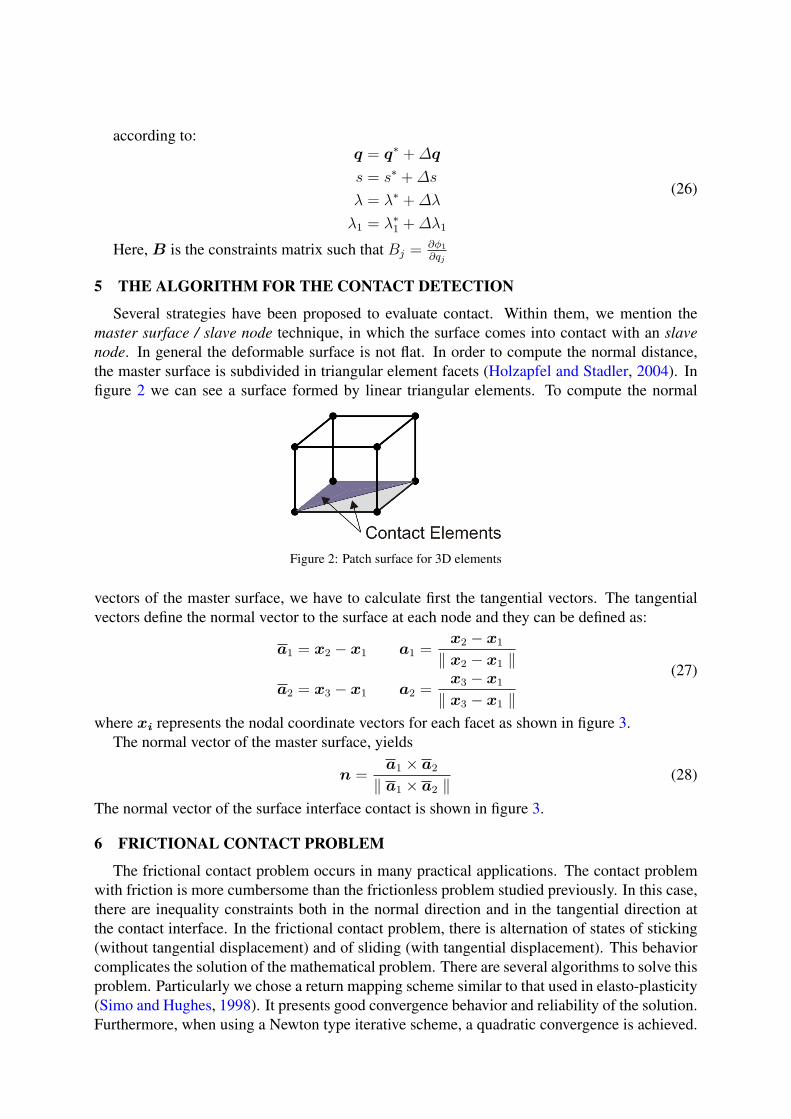
5 THE ALGORITHM FOR THE CONTACT DETECTION

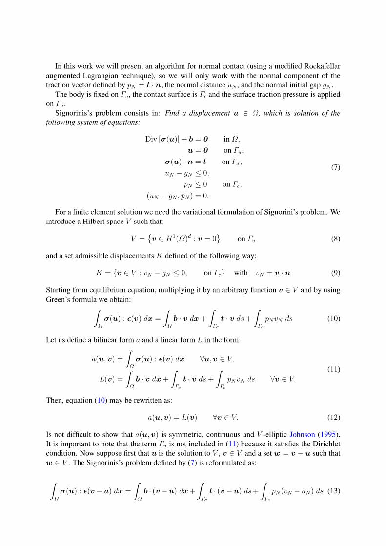
Several strategies have been proposed to evaluate contact. Within them, we mention themaster surface / slave node technique, in which the surface comes into contact with an slavenode. In general the deformable surface is not flat. In order to compute the normal distance,the master surface is subdivided in triangular element facets (Holzapfel and Stadler, 2004). Infigure 2 we can see a surface formed by linear triangular elements. To compute the normal

Figure 2: Patch surface for 3D elements

vectors of the master surface, we have to calculate first the tangential vectors. The tangentialvectors define the normal vector to the surface at each node and they can be defined as:

a1 = x2 − x1 a1 =x2 − x1

‖ x2 − x1 ‖

a2 = x3 − x1 a2 =x3 − x1

‖ x3 − x1 ‖

(27)

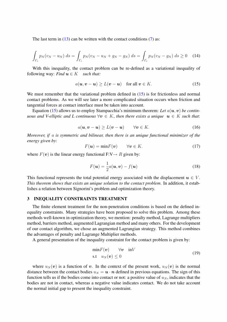
where xi represents the nodal coordinate vectors for each facet as shown in figure 3.The normal vector of the master surface, yields

n =a1 × a2

‖ a1 × a2 ‖(28)

The normal vector of the surface interface contact is shown in figure 3.

6 FRICTIONAL CONTACT PROBLEM

The frictional contact problem occurs in many practical applications. The contact problemwith friction is more cumbersome than the frictionless problem studied previously. In this case,there are inequality constraints both in the normal direction and in the tangential direction atthe contact interface. In the frictional contact problem, there is alternation of states of sticking(without tangential displacement) and of sliding (with tangential displacement). This behaviorcomplicates the solution of the mathematical problem. There are several algorithms to solve thisproblem. Particularly we chose a return mapping scheme similar to that used in elasto-plasticity(Simo and Hughes, 1998). It presents good convergence behavior and reliability of the solution.Furthermore, when using a Newton type iterative scheme, a quadratic convergence is achieved.

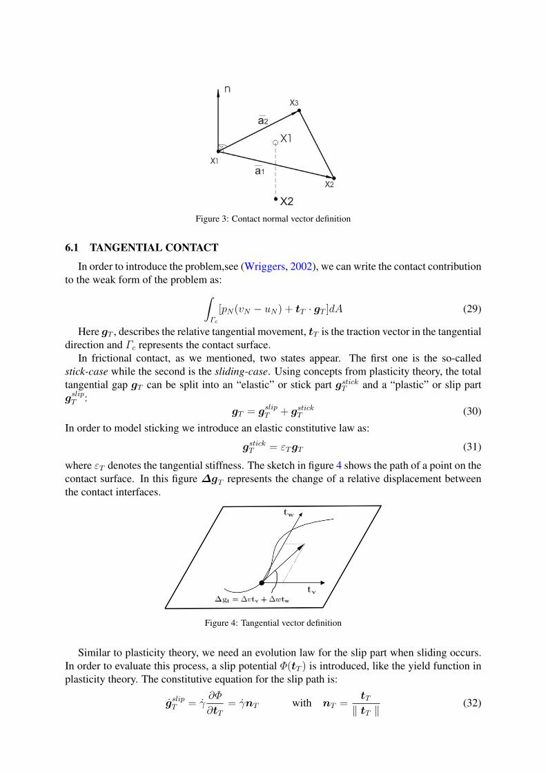
Figure 3: Contact normal vector definition

6.1 TANGENTIAL CONTACT

In order to introduce the problem,see (Wriggers, 2002), we can write the contact contributionto the weak form of the problem as:∫

Γc

[pN(vN − uN) + tT · gT ]dA (29)

Here gT , describes the relative tangential movement, tT is the traction vector in the tangentialdirection and Γc represents the contact surface.

In frictional contact, as we mentioned, two states appear. The first one is the so-calledstick-case while the second is the sliding-case. Using concepts from plasticity theory, the totaltangential gap gT can be split into an “elastic” or stick part gstick

T and a “plastic” or slip partgslip

T :gT = gslip

T + gstickT (30)

In order to model sticking we introduce an elastic constitutive law as:

gstickT = εT gT (31)

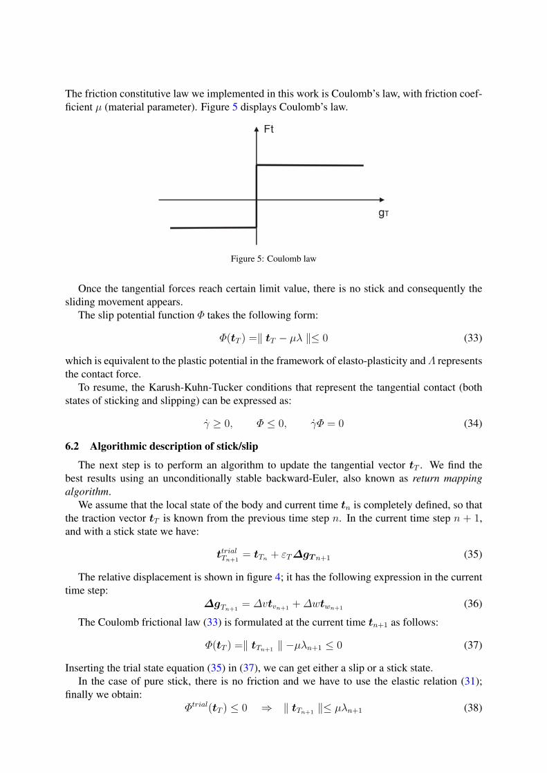
where εT denotes the tangential stiffness. The sketch in figure 4 shows the path of a point on thecontact surface. In this figure ∆gT represents the change of a relative displacement betweenthe contact interfaces.

Figure 4: Tangential vector definition

Similar to plasticity theory, we need an evolution law for the slip part when sliding occurs.In order to evaluate this process, a slip potential Φ(tT ) is introduced, like the yield function inplasticity theory. The constitutive equation for the slip path is:

gslipT = γ

∂Φ

∂tT

= γnT with nT =tT

‖ tT ‖(32)

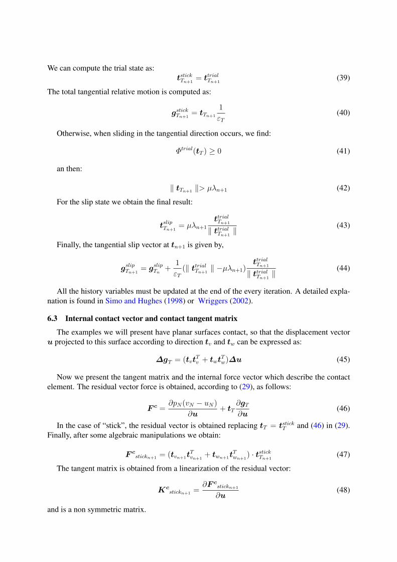
The friction constitutive law we implemented in this work is Coulomb’s law, with friction coef-ficient µ (material parameter). Figure 5 displays Coulomb’s law.

Figure 5: Coulomb law

Once the tangential forces reach certain limit value, there is no stick and consequently thesliding movement appears.

The slip potential function Φ takes the following form:

Φ(tT ) =‖ tT − µλ ‖≤ 0 (33)

which is equivalent to the plastic potential in the framework of elasto-plasticity and Λ representsthe contact force.

To resume, the Karush-Kuhn-Tucker conditions that represent the tangential contact (bothstates of sticking and slipping) can be expressed as:

γ ≥ 0, Φ ≤ 0, γΦ = 0 (34)

6.2 Algorithmic description of stick/slip

The next step is to perform an algorithm to update the tangential vector tT . We find thebest results using an unconditionally stable backward-Euler, also known as return mappingalgorithm.

We assume that the local state of the body and current time tn is completely defined, so thatthe traction vector tT is known from the previous time step n. In the current time step n + 1,and with a stick state we have:

ttrialTn+1

= tTn + εT ∆gT n+1 (35)

The relative displacement is shown in figure 4; it has the following expression in the currenttime step:

∆gTn+1= ∆vtvn+1 + ∆wtwn+1 (36)

The Coulomb frictional law (33) is formulated at the current time tn+1 as follows:

Φ(tT ) =‖ tTn+1 ‖ −µλn+1 ≤ 0 (37)

Inserting the trial state equation (35) in (37), we can get either a slip or a stick state.In the case of pure stick, there is no friction and we have to use the elastic relation (31);

finally we obtain:Φtrial(tT ) ≤ 0 ⇒ ‖ tTn+1 ‖≤ µλn+1 (38)

We can compute the trial state as:tstickTn+1

= ttrialTn+1

(39)

The total tangential relative motion is computed as:

gstickTn+1

= tTn+1

1

εT

(40)

Otherwise, when sliding in the tangential direction occurs, we find:

Φtrial(tT ) ≥ 0 (41)

an then:

‖ tTn+1 ‖> µλn+1 (42)

For the slip state we obtain the final result:

tslipTn+1

= µλn+1

ttrialTn+1

‖ ttrialTn+1

‖(43)

Finally, the tangential slip vector at tn+1 is given by,

gslipTn+1

= gslipTn

+1

εT

(‖ ttrialTn+1

‖ −µλn+1)ttrialTn+1

‖ ttrialTn+1

‖(44)

All the history variables must be updated at the end of the every iteration. A detailed expla-nation is found in Simo and Hughes (1998) or Wriggers (2002).

6.3 Internal contact vector and contact tangent matrix

The examples we will present have planar surfaces contact, so that the displacement vectoru projected to this surface according to direction tv and tw can be expressed as:

∆gT = (tvtTv + twtT

w)∆u (45)

Now we present the tangent matrix and the internal force vector which describe the contactelement. The residual vector force is obtained, according to (29), as follows:

F c =∂pN(vN − uN)

∂u+ tT

∂gT

∂u(46)

In the case of “stick”, the residual vector is obtained replacing tT = tstickT and (46) in (29).

Finally, after some algebraic manipulations we obtain:

F cstickn+1 = (tvn+1t

Tvn+1

+ twn+1tTwn+1

) · tstickTn+1

(47)

The tangent matrix is obtained from a linearization of the residual vector:

Kcstickn+1 =

∂F cstickn+1

∂u(48)

and is a non symmetric matrix.

Using the tangent matrix for the stick state, it results:

Kcstickn+1 = εT (tvn+1t

Tvn+1

+ twn+1tTwn+1

) (49)

Concerning to the sliding process, we will proceed in a similar way. The residual vector isobtained inserting (43) and (44) into (46), and we obtain,

F cslipn+1 = (tvn+1t

Tvn+1

+ twn+1tTwn+1

) · tslipTn+1

(50)

For getting the tangential matrix equation we have to take partial derivatives of the internalvector forces as is shown in (46). After algebra calculus we can express the tangential matrixfor the slip case as:

Kcslipn+1 = µλn+1

ttrialTn+1

‖ ttrialTn+1

‖Bn+ ·An+ ·Bn+ (51)

where,Bn+ = (tvn+1t

Tvn+1

+ twn+1tTwn+1

) (52)

and

An+ = I −ttrialn+1 tTtrial

n+1

‖ tTtrialTn+1

‖2(53)

7 NUMERICAL EXAMPLES

We present two numerical examples where robustness and accuracy of the proposed contactalgorithm are shown. The examples involve quasi-static simulations and were carried-out inthe finite element code OOFELIE. All pre- and post-processing were performed by using thesoftware Samcef Field SAMCEF (2007).

7.1 3D Friction Test. Validation Example

This test represents an important validation for the analysis of friction. The example is pre-sented originally in Armero and Petocz (1999) and Areiras et al. (2004) as a 2D friction test.We compared our 3D results introducing a plane strain state which reproduces the same bound-ary conditions. The mesh topology, boundary conditions and material properties are shown infigure 6.

The material behavior used in this example was linear elastic. We employed a mesh with1583 nodes, 7241 tetrahedron linear finite elements as shown in figure 6. The lateral bound-ary conditions were used to reproduce a plane strain state. A uniform pressure acts on thedeformable body surface and press the flexible body against a rigid foundation. Then, otherpressure actuating on one side of the body pulls it. The deformed configuration for this caseis shown in figures 7 and 8. We can see the same deformation pattern as described in thereferences Armero and Petocz (1999).

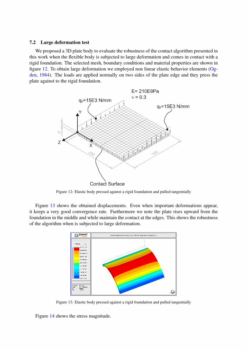
In figures 9 and 10 we plotted the normal and the tangential stresses.Figure 11 shows a comparison of the results in terms of normal and tangential stresses. The

obtained results presents very good agreement with the reference (Armero and Petocz, 1999).

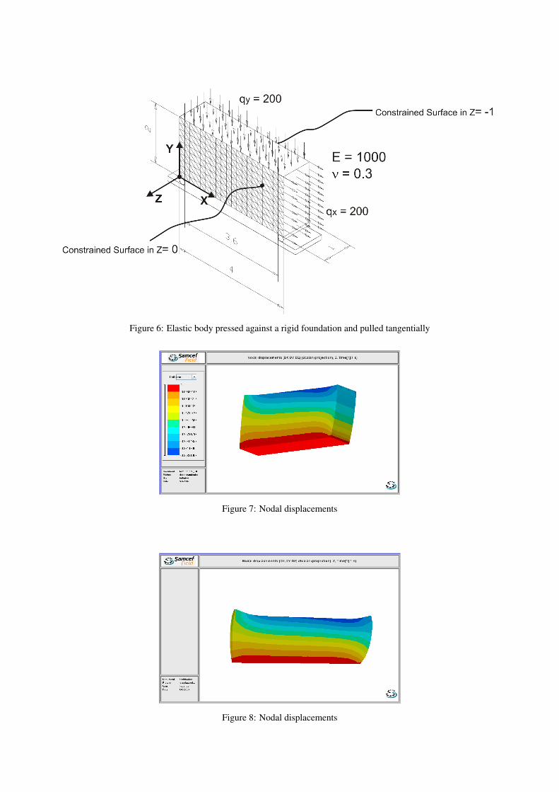
Figure 6: Elastic body pressed against a rigid foundation and pulled tangentially

Figure 7: Nodal displacements

Figure 8: Nodal displacements

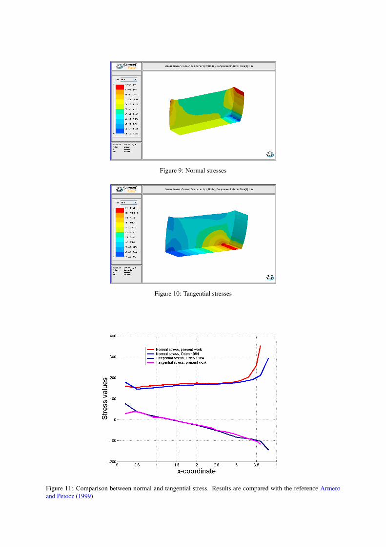
Figure 9: Normal stresses

Figure 10: Tangential stresses

Figure 11: Comparison between normal and tangential stress. Results are compared with the reference Armeroand Petocz (1999)

7.2 Large deformation test

We proposed a 3D plate body to evaluate the robustness of the contact algorithm presented inthis work when the flexible body is subjected to large deformation and comes in contact with arigid foundation. The selected mesh, boundary conditions and material properties are shown infigure 12. To obtain large deformation we employed non linear elastic behavior elements (Og-den, 1984). The loads are applied normally on two sides of the plate edge and they press theplate against to the rigid foundation.

Figure 12: Elastic body pressed against a rigid foundation and pulled tangentially

Figure 13 shows the obtained displacements. Even when important deformations appear,it keeps a very good convergence rate. Furthermore we note the plate rises upward from thefoundation in the middle and while maintain the contact at the edges. This shows the robustnessof the algorithm when is subjected to large deformation.

Figure 13: Elastic body pressed against a rigid foundation and pulled tangentially

Figure 14 shows the stress magnitude.

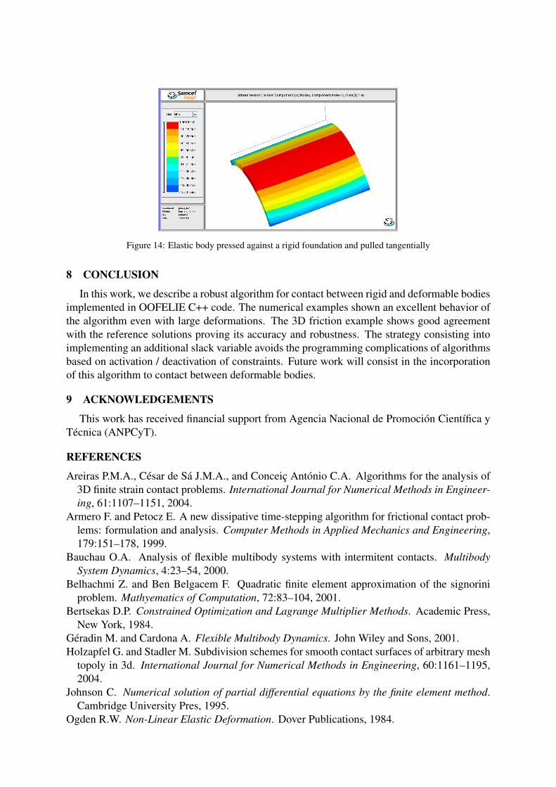
Figure 14: Elastic body pressed against a rigid foundation and pulled tangentially

8 CONCLUSION

In this work, we describe a robust algorithm for contact between rigid and deformable bodiesimplemented in OOFELIE C++ code. The numerical examples shown an excellent behavior ofthe algorithm even with large deformations. The 3D friction example shows good agreementwith the reference solutions proving its accuracy and robustness. The strategy consisting intoimplementing an additional slack variable avoids the programming complications of algorithmsbased on activation / deactivation of constraints. Future work will consist in the incorporationof this algorithm to contact between deformable bodies.

9 ACKNOWLEDGEMENTS

This work has received financial support from Agencia Nacional de Promoción Científica yTécnica (ANPCyT).

REFERENCES

Areiras P.M.A., César de Sá J.M.A., and Conceiç António C.A. Algorithms for the analysis of3D finite strain contact problems. International Journal for Numerical Methods in Engineer-ing, 61:1107–1151, 2004.

Armero F. and Petocz E. A new dissipative time-stepping algorithm for frictional contact prob-lems: formulation and analysis. Computer Methods in Applied Mechanics and Engineering,179:151–178, 1999.

Bauchau O.A. Analysis of flexible multibody systems with intermitent contacts. MultibodySystem Dynamics, 4:23–54, 2000.

Belhachmi Z. and Ben Belgacem F. Quadratic finite element approximation of the signoriniproblem. Mathyematics of Computation, 72:83–104, 2001.

Bertsekas D.P. Constrained Optimization and Lagrange Multiplier Methods. Academic Press,New York, 1984.

Géradin M. and Cardona A. Flexible Multibody Dynamics. John Wiley and Sons, 2001.Holzapfel G. and Stadler M. Subdivision schemes for smooth contact surfaces of arbitrary mesh

topoly in 3d. International Journal for Numerical Methods in Engineering, 60:1161–1195,2004.

Johnson C. Numerical solution of partial differential equations by the finite element method.Cambridge University Pres, 1995.

Ogden R.W. Non-Linear Elastic Deformation. Dover Publications, 1984.

SAMCEF. 2007.Simo J.C. and Hughes T.J.R. Computational Inelasticity. Springer, 1998.Wriggers P. Computational Contact Mechanics. John Wiley and Sons, 2002.