i

Modeling, Simulation and Visualization of Air Pollution Distribution

Using an Advection-Diffusion Model

Syafika Ulfah

A Thesis Submitted in Partial Fulfillment of the Requirements for the Degree of

Master of Science in Applied Mathematics

Prince of Songkla University

2016

Copyright of Prince of Songkla University

ii

Thesis Title Modeling, Simulation and Visualization of Air Pollution

Distribution Using an Advection-Diffusion Model

Author Miss Syafika Ulfah

Major Program Applied Mathematics

Major Advisor Examining Committee:

…………………………… ……………………… Chairperson

( Dr. Somporn Chuai-Aree ) ( Dr. Nifatamah Makaje )

……………………….……………

( Dr. Somporn Chuai-Aree )

……………………….……………

( Dr. Areena Hazanee )

……………………….……………

( Dr. Anurak Busaman )

……………………….……………

( Asst. Prof. Dr. Sanae Rujivan )

The Graduate School, Prince of Songkla University, has approved this thesis as

partial fulfillment of the requirements for the Master of Science Degree in Applied

Mathematics.

…………………………………………

( Assoc. Prof. Dr. Teerapol Srichana )

Dean of Graduate School

ii

iii

This is to certify that the work here submitted is the result of the candidate’s own

investigations. Due acknowledgement has been made of any assistance received.

……………………………. Signature

( Dr. Somporn Chuai-Aree )

Major Advisor

…………………………..... Signature

( Syafika Ulfah )

Candidate

iii

iv

I hereby certify that this work has not been accepted in substance for any other

degree, and is not being currently submitted in candidature for any degree.

……………………….. Signature

( Syafika Ulfah )

Candidate

iv

v

Thesis Title Modeling, Simulation and Visualization of Air Pollution

Distribution Using an Advection-Diffusion Model

Author Miss Syafika Ulfah

Major Program Applied Mathematics

Academic Year 2015

ABSTRACT

Air pollution is an important problem nowadays. Mathematical modeling plays a big

role to research about air pollution. Air pollution modeling is used to study the

behavior of the dispersion of the pollutants in the atmosphere. The advection-

diffusion equation is one of the air pollution models that can be used to describe the

physical processes involved in the dispersal of pollutants in the atmosphere. The

advection-diffusion equation is used in this study to understand how the pollutants

disperse by observing influencing parameters, such as large-scale wind, mesoscale

wind, eddy diffusivity and heat diffusion (temperature). The numerical method that

was used to solve the advection-diffusion equation is the explicit finite difference

method. The solution obtained is simulated and visualized by developing a program

with a simple and interactive user interface using the investigated software namely

“Pollution Distribution Simulation” software written by Lazarus software. The

various parameters in the model are varied to see the influence of the distribution of

pollutants from the simulations. The results show that the large-scale wind, the

mesoscale wind, eddy diffusivity, and heat diffusion have an effect on the distribution

vi

of pollutants in all three conditions of the atmosphere, that are unstable, stable and

neutral conditions.

vii

ชื่อวทิยานิพนธ ์ แบบจ าลอง การจ าลองแบบ และการแสดงภาพของการกระจายตัวของ

มลพิษในอากาศโดยใช้แบบจ าลองการพา-การแพร่

ชื่อผูแ้ตง่ Miss Syafika Ulfah

สาขาวชิา คณิตศาสตร์ประยุกต์

ปีการศกึษา 2558

บทคดัยอ่

มลพิษทางอากาศเป็นปัญหาที่ส าคัญในทุกวันนี้ แบบจ าลองทางคณิตศาสตร์มีบทบาทส าคัญในการท า

วิจัยเกี่ยวกับมลพิษทางอากาศ ซ่ึงถูกน ามาใช้ในการศึกษาพฤติกรรมของการกระจายของสารพิษใน

บรรยากาศ สมการการพา-การแพร่เป็นรูปแบบหนึ่งของตัวแบบมลพิษทางอากาศท่ีถูกใช้ในการ

อธิบายกระบวนการทางกายภาพที่เกี่ยวข้องกับการกระจายของมลพิษในบรรยากาศ สมการการพา-

การแพร่ถูกน ามาใช้ในการศึกษาครั้งนี้เพ่ือสร้างความเข้าใจถึงการกระจายตัวของมลพิษอย่างไรโดย

การสังเกตการปรับเปลี่ยนค่าพารามิเตอร์ เช่น ลมสเกลใหญ่ (large-scale wind) ลมขนาดกลาง

(mesoscale wind) การแพร่กระจายแบบเอ็ดดี้ (eddy diffusivity) และการแพร่ความร้อน

(อุณหภูมิ) วิธีการค านวณเชิงตัวเลขถูกใช้ในการแก้สมการการพา-การแพร่ด้วยวิธีการผลต่างสืบเนื่อง

ชัดแจ้ง ผลเฉลยจากการจ าลองแบบและแสดงภาพถูกพัฒนาด้วยโปรแกรมอย่างง่ายและมีการโต้ตอบ

กับผู้ใช้โดยการใช้โปรแกรมท่ีสร้างข้ึนมาชื่อว่า “Pollution Distribution Simulation” ถูกพัฒนา

ด้วยโปรแกรมลาซารัส พารามิเตอร์ต่างๆ ในตัวแบบจ าลองถูกปรับค่าเพ่ือดูอิทธิพลของการกระจายตัว

ของมลพิษจากการจ าลองแบบ ผลจากแบบจ าลองแสดงให้เห็นว่า ลมสเกลใหญ่ ลมระดับกลาง การ

แพร่กระจายแบบเอ็ดดี้และ การแพร่กระจายความร้อนมีผลกระทบต่อการกระจายตัวของมลพิษทั้ง 3

เงื่อนไขของบรรยากาศ ได้แก่ เงื่อนไขแบบไม่เสถียร แบบเสถียรและ แบบกลาง

viii

Acknowledgements

This thesis would not have been possible without significant contributions and

assistances from a number of people. First and principal, I would like to thank my

supervisor Dr. Somporn Chuai-Aree for his invaluable guidance, support and

assistance throughout the completion of this thesis. Special thanks to all lecturers in

Applied Mathematics program, especially Dr. Rattikan Saelim, Dr. Nifatamah Makaje

Assist. Prof. Dr. Arthit Intarasit, Dr. Areena Hazanee and Dr. Anurak Busaman for

their assistance and guidance. I would like to also thank Emeritus Prof. Dr. Don

McNeil for his enormous contribution and advice.

I would like to acknowledge the Faculty of Science and Technology, Prince of

Songkla University for providing funds through the SAT Scholarships for

International Student of Faculty of Science and Technology. I would like to also

acknowledge the Department of Mathematics and Computer Science and as well as

PBWatch in facilitating this study at Prince of Songkla University, Pattani Campus,

Thailand.

Finally, my sincere thanks go to my family and friends for their encouragement

throughout my study, especially my mother, Mrs. Nurhayati and my friend, Collins

Bekoe.

Syafika Ulfah

ix

Table of Contents

ABSTRACT ................................................................................................................... v

บทคดัยอ่ ............................................................................................................................ vii

Acknowledgements .....................................................................................................viii

Table of Contents .......................................................................................................... ix

List of Figures .............................................................................................................. xii

Chapter 1 ........................................................................................................................ 1

1.1 Background ..................................................................................................... 1

1.2 Problem Statement .......................................................................................... 6

1.3 Motivation ....................................................................................................... 9

1.4 Objectives ...................................................................................................... 12

1.5 Expected advantages ..................................................................................... 12

Chapter 2 ...................................................................................................................... 14

Literature Review ..................................................................................................... 14

Chapter 3 ...................................................................................................................... 21

3.1 Transport of Pollutants in the Atmosphere ................................................... 23

3.2 Derivation of the Advection-Diffusion Equation .......................................... 24

3.2.1 Physical observation of pollutant transport............................................ 24

3.2.2 Mass balance equation ........................................................................... 28

3.2.3 Meteorological factors ........................................................................... 31

x

3.2.4 Boundary and initial conditions of the advection-diffusion equation .... 33

3.3 Finite Difference Method .............................................................................. 34

3.3.1 Forward difference method .................................................................... 35

3.3.2 Backward difference method ................................................................. 36

3.3.3 Central difference method...................................................................... 37

3.3.4 The explicit finite difference scheme ..................................................... 37

3.4 Numerical Solution of the Proposed Mathematical Model ........................... 39

3.4.1 The advection-diffusion equation .......................................................... 39

3.4.2 Temperature ........................................................................................... 42

3.4.3 Parameters involved in the advection-diffusion equation ...................... 43

3.5 The Proposed Modeling of Air Pollution Distribution ................................. 45

Chapter 4 ...................................................................................................................... 46

4.1 User Interface of the “Pollution Distribution Simulation” Software ............ 47

4.2 Simulation ..................................................................................................... 54

4.3 Visualizing the Effects of the Model Parameters on the Concentration of

Pollutants .................................................................................................................. 59

Chapter 5 ...................................................................................................................... 72

5.1 Conclusion ..................................................................................................... 72

5.2 Further research ............................................................................................. 73

References .................................................................................................................... 74

APPENDIX .................................................................................................................. 79

xi

How to use the program? ......................................................................................... 80

Algorithm of the program ........................................................................................ 82

Vitae ............................................................................................................................. 90

xii

List of Figures

Figure 1. Stability of an object. ...................................................................................... 2

Figure 2. Air parcel in the atmosphere. .......................................................................... 3

Figure 3. A simplified model of environmental pollution (Holdgate, 1979). ................ 4

Figure 4. Work flow. .................................................................................................... 22

Figure 5. Transport of pollutants in the atmosphere. ................................................... 24

Figure 6. An air mass through an ellipse. .................................................................... 25

Figure 7. Diffusion process in a flux ........................................................................... 26

Figure 8. Domain. ........................................................................................................ 34

Figure 9. Explicit finite difference scheme. ................................................................. 38

Figure 10. User interface of the program. .................................................................... 47

Figure 11. Parameter adjusting panel........................................................................... 48

Figure 12. Atmospheric condition panel. ..................................................................... 48

Figure 13. Initial value panel ....................................................................................... 49

Figure 14. Arbitrary point panel .................................................................................. 49

Figure 15. Model parameters panel. ............................................................................ 50

Figure 16. Visualization panel. .................................................................................... 51

xiii

Figure 17. Graph panel. ............................................................................................... 52

Figure 18. Execution buttons. ...................................................................................... 52

Figure 19. Check boxes panel. ..................................................................................... 53

Figure 20. Graphic value panel. ................................................................................... 53

Figure 21. Initial value panel. ...................................................................................... 55

Figure 22. Position of the arbitrary point. .................................................................... 55

Figure 23. Parameters values for simulation................................................................ 56

Figure 24. Pollutants distribution in all atmospheric conditions. ................................ 56

Figure 25. The parameters value for simulation when the large-scale wind is

increased. ..................................................................................................................... 57

Figure 26. Varying mean wind speed in all atmospheric condition. ........................... 58

Figure 27. Pollutant distribution by varying the large-scale wind. .............................. 59

Figure 28. Visualization of pollutants distribution with positive large-scale wind. .... 61

Figure 29. Visualization of pollutants distribution with negative large-scale wind. ... 62

Figure 30. Pollutant distribution by varying the heat diffusion. .................................. 62

Figure 31. Pollutant distribution by varying air flow. ................................................. 63

Figure 32. Pollutant distribution by varying mesoscale wind...................................... 65

xiv

Figure 33. Visualization of pollutants distribution with positive mesoscale wind

0.3 .m s ........................................................................................................................ 67

Figure 34. Visualization of pollutants distribution with positive mesoscale wind

0.3 .m s ..................................................................................................................... 68

Figure 35. Pollutant distribution by varying diffusion rate.......................................... 69

Figure 36. Visualization of pollutants distribution with diffusion rate of 20.6 .m s ... 70

Figure 37. Visualization of pollutants distribution with diffusion rate of 20.6 .m s ... 71

xv

List of Tables

Table 1. Stability and surface roughness constants. .................................................... 46

Table 2. Varying large-scale wind ............................................................................... 60

Table 3. Varying heat diffusion rate ............................................................................ 63

Table 4. Varying air flow ............................................................................................. 64

Table 5. Varying mesoscale wind. ............................................................................... 66

Table 6. Varying diffusivity. ........................................................................................ 69

1

Chapter 1

Introduction

In this research, modeling and simulation of air pollution distribution is presented. In

this chapter, the problems and motivations of the research are enlightened. Moreover,

the aims of the research are stated as well.

1.1 Background

Environmental issues are gaining an ever-increasing attention at local, national and

international levels. Parts of the problems and challenges facing governments and

institutions alike is choosing and coming up with strategies and plans to maintain a

safe environment.

Pollution as an inevitable product of all industrial economies is a price for a way of

life and it can generally be defined as the introduction and accumulation of

contaminants into the environment. These are as a result of buildup of waste and

unwanted materials which comes from the activities of living organisms and can be

classified as artificial or man-made. The contaminating substances can also be from

natural processes such as metal accumulation from rock dissolution but the most

extreme and more severe examples of pollution, however, are usually associated with

or caused by human activities. Although environmental pollution has been an

alarming issue throughout the history of man and in the latter part of the century, little

has been done to curb it.

2

Air pollution is one of the major atmospheric problems currently facing the world

today. It is the introduction of undesirable substances into the air in an enormous

amount to cause health issues (Noel de Nevers, 2000). Meanwhile, the World Health

Organization (WHO) defines air pollution as the contamination of the indoor or

outdoor environment by any chemical, physical or biological agent that modifies the

natural characteristics of the atmosphere. Various studies have shown the effects of

polluted air on agricultural productivity, the ecosystem, and human health.

The environment as we know is made of the atmosphere, the soil, water bodies and

these play an important role in the emission of pollutants. Pollutants are always

deposited in these parts of the ecosystem. The emitted pollutants undergo chemical

and physical changes through interactions with the environment.

Air is a multicomponent mixture of gaseous molecules and atoms which are

constantly moving about and undergoing frequent collisions. The ability of the

atmosphere to reflect or absorb the concentration of pollutants depends on

meteorological factors such as temperature, humidity level, pressure, wind velocity,

etc. as well as the state of the atmosphere whether unstable, stable or neutral.

Figure 1. Stability of an object.

Unstable

Stable

Neutral

3

Figure 2. Air parcel in the atmosphere.

Figure 1 shows the concept of stability of an object. The unstable, stable, and neutral

state of the object can be explained with the object coming back to a state of equilibrium

after any movement. Under the unstable state, the object does not come back to an

equilibrium state but otherwise in the case of the stable state. In the neutral state the

object remains until it is further displaced.

This concept can be used to understand atmospheric stability conditions. Figure 2 shows

an air parcel in the atmosphere. The air parcel is said to be in an unstable state if the

temperature of the surrounding air is greater than the temperature of the air parcel. In

other words, the parcel of air becomes less dense and then moves in the upward

direction. In a stable state, the air parcel moves in the downward direction when the

temperature of the surrounding air becomes less than the temperature of the air parcel.

This means that the parcel is heavier than the surrounding air and therefore it would

sink. The air parcel is said to be in the neutral state when the temperature of the

Tair

Tparcel

Tair

Tparcel

Unstable

T parcel > T air

Parcel is lighter and

moves up.

Stable

T parcel < T air

Parcel is heavier and

moves down.

Neutral

T parcel = T air

Parcel stays put.

Tair

Tparcel

4

surrounding air is equal to the temperature of the air parcel. This means that the air

parcel would remain at where it is until the conditions in the atmosphere change. These

atmospheric conditions determine how long pollutants remain in the atmosphere

whether they would be absorbed or reflected in the atmosphere in the short or long term.

The pollution pathway concept described by Holgate (1979) is a convenient way for

studying and appreciating the distribution of the concentration of pollutants. Holdgate

(1979) stated that there are common characteristics associated with pollutant

emissions. These include the pollutants themselves (𝑁𝑂𝑥, 𝑆𝑂2, 𝑒𝑡𝑐. ), the source of the

pollutants (industrial stacks, fumes from automobiles), medium of transport (either

through air, water or soil) and the receptors (the living organisms, ecosystems or

items or buildings affected by the pollutants).

The distribution of pollutants can be clearly explained by other variables including the

rate of emission of the pollutants from the source, the rate of the transport, physical

TARGET

Transfer within

Target organism

Target organism

Excretion of pollutant

or derivative

Deposition/removal

during transport

TRANSPORT

Rate of transport

Source of

pollutant

P

O

L

L

U

T

A

N

T

Rate of emission

of pollutant Amount of

pollutant

reaching target

(in air, water or soil)

Chemical transformations

in environmental media

Figure 3. A simplified model of environmental pollution (Holdgate, 1979).

5

and chemical transformations which the pollutants undergo either during transport or

after deposition at the target, amounts reaching the target and its effects on the target.

Sources of pollutants can either be discrete point sources or area point sources. During

pollutants emission, they are distributed through the environment either in the air (e.g.

smoke, 𝑁𝑂𝑥, 𝑆𝑂𝑥), in water (e.g. industrial effluents) or in soil. Therefore, the

transport mechanisms include movement in wind and water, gravity, and other

anthropogenic transport media. Most air pollutants are released in the part of the

atmosphere that is close to the earth surface (boundary layer) where normally wind

blows due to turbulence. Larger particulates of pollutants of about 1 − 10 𝜇𝑚 are

deposited in the boundary layer while smaller particles (mostly gaseous) that are

normally less than 5 𝜇𝑚 are transported into the part which is mostly the earth’s

atmosphere (troposphere). These transports are as a result of the vertical movements

of thermal plumes which are carried by high winds and storms that flow over

mountains. Climatic changes in the atmosphere and particles size also have an effect

on the transport of pollutants.

On the boundary layer, there is a continuous mixing of pollutants and the surrounding

air until they attain a relatively uniform concentration. Wind velocity, solar radiations,

land surface roughness and the cloud are some of the factors that determine how the

concentration of pollutant dilute in the atmosphere (Masters, 1991).

The density of air is inversely proportional to its temperature and therefore warm air

is less dense and rises, while cooling air becomes denser and descends. The adiabatic

lapse rate (the decrease in atmospheric temperature with rising altitude) of the cooling

of air masses plays a major part in determining the stability of the air into which

6

pollutants are released. If the temperature of rising warm air decreases at a rate faster

than the adiabatic lapse rate, dilution of pollutant concentration occurs as the air mass

becomes unstable. However, if the temperature drops more slowly than the adiabatic

lapse rate, the concentration of the pollutants would increase as the air becomes

stable.

The reduction in the concentration of the pollutants depends largely on the velocity of

the wind and the how far the pollutants can rise into the atmosphere. In other to

explain the principal factors involved in the emission and the dispersion of pollutants,

it would be convenient to use an example of the dispersion of plume of smoke from a

single chimney since many atmospheric pollutants are emitted from industrial stacks

(chimneys). It is also important to realize that the presence of tall buildings, other

chimneys, and the urban environment can greatly complicate the pattern of dispersion

of atmospheric pollutants from a single chimney.

Most models of time-averaged concentrations of pollutants downwind from a point

source, such as chimney are based on a normal (Gaussian) distribution curve of the

pollutants. In this research, the advection diffusion equation with time-dependent

would be used to study how pollutants disperse and diffuse in the atmosphere. Some

atmospheric parameters would be considered.

1.2 Problem Statement

As stated earlier, pollution has been a major problem facing governments and world

leaders for decades now. The pollution problem can be viewed as affecting the quality

of air, oceans and water bodies and to a large extent the ecosystem. The polluted air

7

can affect human health and other living things. It can have a global consequence like

acid rain and global warming.

WHO reported that in 2012, air pollution exposure was responsible for 7 million

premature deaths, and this occurs annually. The United State Environmental

Protection Agency (EPA) in 2009 reported that emissions of carbon dioxide and other

long-lived greenhouse gasses that build up in the atmosphere harm the health and

welfare of current and future generations by causing climate change and ocean

acidification.

Ocean acidification issues occurred in Oregon as Kristin Eberhard reported. She

stated that pollution has infiltrated Oregon’s coasts and has caused acidification. This

has created problems for the Ocean’s shellfish industry. The ocean acidification

reduces the pH causing high acidity which reduces the carbonate ions concentration

useful to form shells of marine animals such as crab. This condition causes their shells

to become fragile and makes them vulnerable.

In the economic aspects, huge sums of money are spent on air pollution issues. In

China, to prevent and plan control action of the airborne pollution, it would be backed

by 1,700 billion yuan ($277 billion) in total investment from the central government

(China Daily, 2013).

The sources of pollution whether it is affecting the quality of air or water bodies are

normally from either natural phenomenon or anthropogenic sources. In the natural

phenomenon, volcanic ash, forest fires (due to excessive drought, El Nino) etc. can

contribute to air pollution. As an example, on June 2015, Raung mount, one of the

8

active volcanoes in Indonesia erupted; it is located in the province of East Java and its

2-kilometres-wide and 500-metres-deep. This mount shot out ash around 1,000 meters

into the air. As a result, several airports were closed because of the decreasing

visibility.

In anthropogenic sources, emissions occur from industrial stacks, vehicle combustion

and sometimes forests fires. Forest fires normally occur in countries like Indonesia

because of land clearing for oil palm plantations. Large acres of land are set ablaze in

an attempt to clear the land and prepare it for the next planting season. Forest fires in

Indonesia is a local problem has extended to a global consequence. They result in the

emissions of carbon and because of that, it needs to be prevented. One of the foreign

exchange earners in Indonesia is oil palm production and because of that, it becomes

difficult to handle, as it is a profitable and an important commodity. Air pollution

problem that has been occurring recently is from forest fires in Sumatra and this issue

can be caused by either anthropogenic or natural causes. Jakarta Post reported that

heavy smoke from the fires in Sumatra island has caused levels of air pollutants to

spike throughout islands and some parts of Malaysia, Singapore, and even Thailand.

The major concerns are that people were dying from inhaling the smoke coming out

of the burning forests. Also, the blaze is destroying forests that are the lungs of the

world.

El Nino in 2015 is responsible for many fire outbreaks. This phenomenon made the

atmosphere warm and dry thereby increasing the number of fire outbreaks in countries

like Indonesia. Many of these fires come from lands which are rich in carbon. There

are a lot of peat reserves and when there is a fire outbreak, they produce huge dark

9

smoke with carbon dioxide and other greenhouse emissions. These contribute to

climatic problems. Sumatra, Indonesia might seem a world away but the haze from

the fires there travel miles bringing that smoke and its accompanying degraded air

quality across the globe.

Industrial stacks, a medium to release air pollutants like sulfur dioxide and nitrogen

oxides rise into the atmosphere from the burning of coal in an effort to disperse

pollution and decrease the impact on the local community has in the long term

become a mirage. This is because wind currents are faster at higher altitudes, causing

pollution to travel hundreds of miles to surrounding provinces, states, and cities.

These pollutants are released into the atmosphere during the burning of fossil fuels

and when it rains, the water droplets combine with these air pollutants and as a result,

become acidic and then falls to the ground in the form of acid rain which can cause

severe damage to humans, animals, and crops.

1.3 Motivation

Life cannot be separated from air, without it living organisms including humans

would not survive. Living organisms have to breathe and accept the air as it exists in

the atmosphere. We cannot choose which air to be breathe.

Every country in this world experiences the pollution problem in their cities. The

distinguishing feature is the level of pollution in each country which depends on how

they manage their air quality. Air pollution in high levels can affect humans,

ecosystem or the climate.

10

Pollution, as we know, consist of contaminants which have undesired effects. Those

contaminants are 𝑁𝑂𝑥, 𝑆𝑂2, 𝐶𝑂, 𝑃𝑀, 𝐶𝑂2 and much more. Almost all respiratory

diseases are caused by air pollution exposure. For instance, carbon monoxide 𝐶𝑂 can

prevent oxygen from entering the various body organs of the body and tissues, 𝑃𝑀2.5

and 𝑃𝑀10 that may be inhaled will most likely be able to be deposited within the

lungs and bloodstream because of their small size. Another effect of air pollution

exposure is that pollution can damage the ecosystem. The ocean acidification issue is

one of the problems caused by air pollution exposure which damages the aquatic

ecosystem. It is the decrease in the pH of earth’s oceans. This is usually caused by the

increase in carbon dioxide in the atmosphere produced by human activities (like fossil

burning). Air pollution can even change the climate. 𝐶𝑂2, 𝐶𝐻4, 𝑁2𝑂 contribute to

greenhouse gasses. The particles in the haze can reflect and absorb incoming solar

energy. Consequently, the atmosphere becomes warm.

With the underlying effect and consequences, it is important to study the distribution

of air pollution in order to know the dispersal or transport of pollutants. One of the

factors affecting air pollutants distribution is air flow. Without currents of wind, the

air pollutants will stick around the source of emission and as a result become

increasingly concentrated, but a meteorological cycle of weather has an enormous

effect on pollutants distribution and either at high or low levels it can alter the

diffusion and advection processes of pollutants.

Weather refers to the state of the atmosphere with respect to the wind, temperature,

pressure, humidity, etc. The pollutants can go as far as the wind carries it. Advection

transports pollutants in the downwind direction and it can transfer the pollutants far

11

away from the source of emissions. As the pollutants are being dispersed, they diffuse

with time as well. Temperature, pressure, and humidity affect the diffusion process of

pollutants. When the temperature is high, it increases the energy, consequently, the

pollutants concentration diffuses faster than when the temperature is low. As the

temperature is proportional to the atmospheric pressure, pollutants diffusion becomes

faster at high pressures and slower in low-pressure conditions. When the atmosphere

is very humid, it has more density, consequently, the pollutants concentration diffuses

slowly.

There are some studies on the effect of 𝑁𝑂𝑥, 𝑆𝑂2, 𝐶𝑂, 𝑃𝑀, 𝐶𝑂2 and other

contaminants on human health. Zulkarnain, et.al., (2010) did a study on the effect of

air pollution on respiratory health and the cost of associated illness. There are lack of

studies on these emission problems on modeling and simulation. Virtually, the study

on this view can predict and or estimate the concentration of pollutants and how far it

is distributed. There is the need to study this in order to know how the pollutants

distribute in the atmosphere. Thus, this study would simulate the distribution of the

pollutants by examining the meteorological parameter involved such as wind

direction, wind velocity and eddy diffusivity using the simulated data.

In this research work, questions like is the pollutant being emitted from a point source

and in low levels over a large area (non-point source) will be answered and thereby

formulate procedures either to stop production of the pollutant or to reduce its

concentration in the environment by finding other methods of manufacturing or waste

handling.

12

As we know, not only does advection carries pollutants away in downwind direction

and transport it as long as the wind blows, but diffusion also aids in the movement of

the pollutants. We would, therefore, present an advection-diffusion model to describe

air pollution distribution.

1.4 Objectives

The objectives of this research are:

1.1 To study air pollutants distribution using an advection-diffusion model.

1.2 To simulate the proposed mathematical model numerically by explicit finite

difference method.

1.3 To create a program for simulation and visualization of air pollution

distribution.

1.4 To analyze the distribution of air pollution in unstable and stable

atmospheric conditions.

1.5 Expected advantages

The research work would be beneficial in the following ways.

1.1 An advection-diffusion model can help to understand the distribution of

pollutants as they are dispersed through advection and diffusion processes.

1.2 The explicit finite difference method is intuitive and easy to implement to

provide a quicker way of solving the proposed model which would help in

the simulation of the pollutants for visualization.

1.3 A computer program would provide a way of altering the various parameters

for visualization to know how the pollutants disperse.

13

1.4 Pollutants disperse differently in different atmospheric conditions and

therefore analyzing how they disperse in these conditions would help in

better policy making by governments.

Research work related to this study would be discussed in the next chapter.

14

Chapter 2

Literature Review

The main goal of this chapter is to relate the present study in the context of other

studies and related work of air pollutants distribution modeling.

Pollution is the most serious of all environmental problems and poses a major threat

to the health and well-being of millions of people and global ecosystems. For at least

thirty years, people have become increasingly aware of these issues. As a result,

governments and regulatory bodies have responded by taking action against grossly

polluting activities in the emission of pollutants into the environment.

However, mathematicians on the other hand have approached the pollution problem

through modelling of the real world situation by considering the pollutants

themselves, the source of emission, the receptors (people, building, ecosystem) and

how the pollutants distribute in the atmosphere and also the effects meteorological or

climatic parameters or factors have on the dispersal or distribution of pollutants from

a region of higher concentration to a region of lower concentration.

Quantification of the relationships between emissions and concentrations involves

two steps: identifying what the most important atmospheric processes are, and

representing these mathematically in a model (Bell and Treshow, 2002).

Mathematical models are useful to study how pollutants behave when there are new

sources of air pollution or changes in a number of pollutants emitted into the air from

the presence of emission sources and help in analyzing such behaviors (Awasthi,

15

Khare, and Gargava, 2006). Mathematical formulations of transport and dispersion

are developed to identify the parameters of interest. Air quality models have become

integrated tools in environmental monitoring, management and assessment of air

pollution (Fenger and Tjell, 2009). The perfect air pollutant concentration model

would allow us to predict the concentrations that would result from any specified set

of pollutant emissions, for any specified meteorological conditions, at any location,

for any time period, with total confidence in the prediction (de Nevers, 2000). A study

by Arystanbekova (2004) stated that simulation of air pollution is useful in providing

information about the spreading of pollutants in an area, the scale, and level of

pollution and estimation.

Venkatachalappa, Khan, and Kakami (2003) studied a time-dependent two-

dimensional advection-diffusion model of air pollution for an area source with an

equation of the primary pollutant as follows:

,p p p

z wp p

C C CU z K z k k C

t x z z

where , ,

p pC C x z t is the

ambient crosswind integrated concentration of pollutant species, U is the mean wind

speed in x direction, z

K is the turbulent eddy diffusivity in zdirection, wp

k is the

first order rainout/washout coefficient of primary pollutant p

C , and k is the first

order chemical reaction rate coefficient of primary pollutant p

C . The concentration

for the secondary pollutant is ,s s s

z ws s g p

C C CU z K z k C v kC

t x z z

where , ,s s

C C x z t is the secondary pollutant, ws

k is the first order wet deposition

coefficient of secondary pollutants, and g

v is the mass ratio of the secondary

16

particulate species to the primary gaseous species which is being converted. The

parameters they considered were variable wind velocity, eddy diffusivity, and

chemical reaction. The model was solved by the implicit Crank-Nicolson finite

difference technique. The model analyzed primary and secondary pollutants in stable

and neutral atmospheric conditions. The result showed that the ground level

concentration of primary pollutants attains peak value at the downwind end of the

source region whereas, the concentration of secondary pollutants attains its peak value

at the source free region in the downwind direction. The model also predicts that the

ground level concentration of a secondary pollutants at a particular downwind

distance is always higher in the stable atmospheric condition than that of the neutral

atmospheric condition.

Sudheer, Lashminarayanachari, Prasad and Pandurangappa (2012) studied a two-

dimensional mathematical model to analyze air pollutant distribution emitted from an

area source. In the study, they considered chemical reaction and dry deposition for

primary and secondary pollutants, with the equation of primary pollutant as follows:

,p p p

z p

C C CU z K z kC

t x z z

and for secondary pollutant,

.s s s

z g p

C C CU z K z v kC

t x z z

The model was solved numerically by

using the implicit Crank-Nicolson finite difference technique. The results showed that

the ground level concentration increases in the downwind distance within the source

region and then decreases rapidly in the source free region to an asymptotic value.

They noticed that the effect of deposition velocity, gravitational settling, and chemical

17

reaction rate coefficients on primary and secondary pollutants reduces the

concentration in the urban region.

Agarwal and Tandon (2009) presented a steady state two-dimensional mathematical

model to study the dispersion of air pollutants. They considered mesoscale wind

which is generated by urban heat island with the following equation

1,

z e

e

C C CK C w

x u u z z z

where C is the air pollutant concentration

at any location ,x z , u is the large-scale wind in the horizontal x direction, e

u and

ew are the mesoscale wind components in the x and z direction respectively,

zK is

eddy diffusivity coefficient in zdirection, and is a first order constant depletion

parameter that defines the fractional loss of pollutant per unit time through various

wet deposition processes existing in the atmosphere. The model is solved numerically

by the implicit Crank-Nicolson finite difference scheme. The results showed that the

mesoscale wind aid the pollutants to circulate and move in the upward direction, thus

making the problem of air pollution more severe in urban areas.

Suresha, Lakshminarayanachari, Prasad and Pandurangappa (2013) studied a two-

dimensional advection-diffusion mathematical model on pollutant distribution, with

the equation of primary pollutant as follows:

,p p p

z p

C C CU z K z kC

t x z z

and for secondary pollutant

,s s s s

z s g p

C C C CU z K z W v kC

t x z z z

where

sW is the gravitational

settling velocity. They solved the model by using the implicit Crank-Nicolson finite

18

difference technique by considering chemical reaction and gravitational settling. The

results showed that the concentration of primary and secondary pollutants decreases

as the removal mechanisms such as dry deposition and gravitational settling velocity

increases for stable and neutral cases.

Pandurangappa, Lakshminarayanachari, and Venkatachalappa (2012) presented a

two-dimensional numerical model for the dispersion of air pollutants. The study was

done to find out the effect of mesoscale wind on the emission of pollutants from an

area source, with the equation of the primary pollutant as follows:

, ,p p p p

z wp p

C C C CU x z W z K z k k C

t x z z z

where W is mean

wind speed in zdirection, and for the secondary pollutant,

, .s s s s s

z s ws s g p

C C C C CU x z W z K z W k C v kC

t x z z z z

The study

was done for primary and secondary pollutants with gravitational settling velocity.

The model was solved numerically using the implicit Crank-Nicolson finite difference

method. The results showed that in the presence of mesoscale wind, the concentration

of primary and secondary pollutants is less on the upwind side of the center of heat

island and more on the downwind side of the center of heat island. It is not the case in

the absence of mesoscale wind. This is because the mesoscale wind increases the

velocity in the upwind direction and decreases in the downwind direction of the center

of the heat island.

Lakshminarayanachari, Suresha, Siddalinga, and Pandurangappa (2013) presented a

numerical model on air pollutants emitted from an area source. In the study, they

19

considered primary and secondary pollutants with chemical reaction and gravitational

settling with point source on the boundary. They analyzed the dispersion of air

pollutants in an urban area in the downwind and vertical direction, with the equation

of primary pollutant as follows: ,p p p

z p

C C CU z K z kC

t x z z

and for

secondary pollutant, .s s s s

z s g p

C C C CU z K z W v kC

t x z z z

Stable and

neutral atmospheric conditions were considered in the presence of large scale wind.

The study showed that removal mechanisms play an important role in reducing the

concentration of pollutants everywhere in the region except near the point source.

Again, they showed that stable atmospheric condition is unfavorable for animals and

plants in a polluted environment.

Lakshminarayanachari, Sudheer, Siddalinga, and Pandurangappa (2013) presented

advection-diffusion numerical model of air pollutants emitted from an urban area

source. They considered chemical reaction and dry deposition as their parameters.

This was done for primary and secondary pollutants by plotting concentration

contours, with the equation of primary pollutant as follows:

,p p p

z p

C C CU z K z kC

t x z z

and for secondary pollutant,

.s s s

z g p

C C CU z K z v kC

t x z z

Their results showed that the removal

mechanisms play an important role in reducing the concentration of the pollutants

everywhere in the city region except near the point source.

20

Pollutants emission are governed by meteorological parameters as they undergo

advection and diffusion process in the atmosphere. Meteorological parameters like

temperature and wind speed have been shown to be factors that influence the

dispersion of pollutants in the atmosphere. A study by Verma and Desai (2008)

showed the effect of meteorological conditions on air pollution in Surat city, India.

The meteorological conditions considered were wind speed, wind direction, and

temperature. The result showed that as wind speed and temperature are high, the

dispersion is high. Therefore, it was concluded that wind speed is the major parameter

that affects the dispersion of pollutants.

Hosseinibalam and Hejazi (2012) investigated the influence of meteorological

parameters on air pollution. The study was done in Isfahan, Iran, and the meteorological

parameters that were observed are wind speed, temperature, air pressure and sunshine

hours. The result showed that high air pollutions in December are due to low sunshine,

no wind, and high atmospheric pressure.

The methodology that would be employed in solving the advection-diffusion model

would be shown in Chapter 3.

21

Chapter 3

Methodology

This chapter presents the mathematical model that would be used to study the

distribution of pollutants in the atmosphere. When the pollutants disperse in the

atmosphere, some physical and removal processes like advection and diffusion take

place irrespective of the atmospheric conditions.

The mathematical model for this study would be formulated by deriving the

advection-diffusion model with some assumptions to clearly explain how the

parameters used in the model behave. Numerical methods for solving the model

would be the finite difference scheme either the explicit or implicit method. The

forward, the backward and the central difference schemes are used to solve the

boundary value in order to approximate the proposed model.

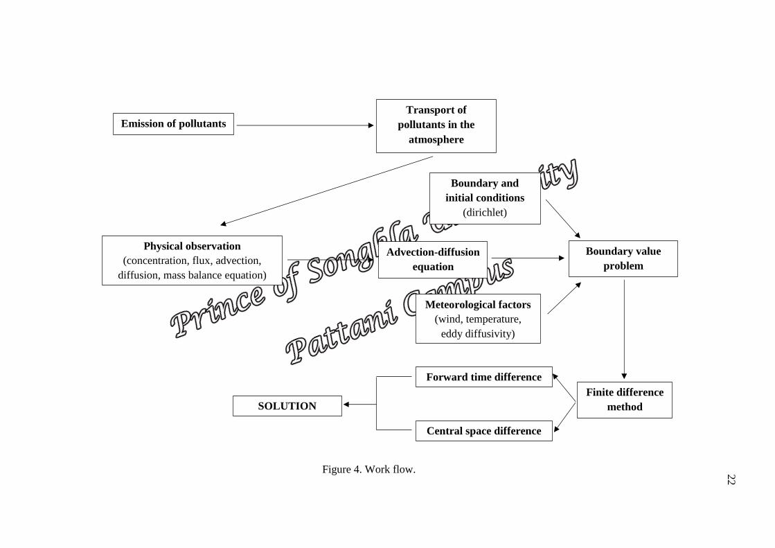
Figure 4 shows the work flow of this study. This starts with the emission of pollutants

from sources like industrial stacks, automobiles, forest fires, etc. The pollutants are

then transported and distributed through advection and diffusion processes. Advection

is as a result of the wind and diffusion is when the pollutants move from a region of

high concentration to a region of low concentration. This phenomenon can be

modeled mathematically using an advection-diffusion equation taking into account

meteorological factors like wind, temperature and eddy diffusivity. This is a boundary

value problem which is coupled with initial and boundary conditions. The finite

difference method is used to find the numerical solution of the advection diffusion.

22

Emission of pollutants

Transport of

pollutants in the

atmosphere

Physical observation

(concentration, flux, advection,

diffusion, mass balance equation)

Advection-diffusion

equation

Boundary and

initial conditions

(dirichlet)

Meteorological factors

(wind, temperature,

eddy diffusivity)

Boundary value

problem

Finite difference

method

Forward time difference

Central space difference

SOLUTION

Figure 4. Work flow. 22

23

3.1 Transport of Pollutants in the Atmosphere

When pollutants are released from the source of emission, either through the soil,

water or air, it disperses through advection, diffusion, and other dispersion

mechanisms. Advection transports the pollutants in the downwind direction by wind.

It can carry the pollutants from the source of emission through the mass movement

from the area which is of high-pressure to a low-pressure area. Naturally, wind speeds

increase with increasing height and thus results in the difference of dilution of

pollutants concentration at a different height. Therefore, it is one of the factors that

determines how fast the pollutants dilute in the atmosphere.

The diffusion process usually occurs in two ways. The first is molecular diffusion,

which occurs due to the random motion of molecules within the fluid. The second is

turbulent diffusion, which is the mixing due to turbulent motions in the fluid

(Ramaswami, Milford, and Smal, 2005).

Most air pollutants are released into the boundary layer where they mix with the

surrounding air. This surrounding air is the interaction between air flow with the

surface roughness of the Earth’s surface. This results in turbulence, which then results

in the decrease in pollutants concentration. The degree of turbulence control how

much the air pollutants dilute in the atmosphere.

The factors that determine the degree of turbulence are incoming solar radiation, wind

speed, cloud cover and surface roughness. The temperature of the air also determines

how much water vapor the atmosphere can hold and the form of clouds it can form. In

general, surface roughness and atmospheric conditions need to be taken into account

24

(Jakeman, Beck, and McAlee, 1995). These conditions aggravate wind speed at

ground level and at higher altitude. In the atmosphere, the atmospheric condition is

categorized by three cases. The cases are an unstable, neutral and stable condition.

These atmospheric conditions would result in the difference in the pattern of the puff

of smoke. Consequently, it results in the varying of the diffusion capability.

Figure 5. Transport of pollutants in the atmosphere.

Figure 5 describes the transport of pollutants in the atmosphere right from the source

of emission through to the transport by advection coupled with turbulence and finally

the effect on receptors, that is the living organisms, ecosystem, building, etc.

3.2 Derivation of the Advection-Diffusion Equation

3.2.1 Physical observation of pollutant transport

The application of the conservation of mass equation to the analysis of physical

systems is essential for studying materials leaving and entering a system. What this

25

means is that if the level of pollutants in the atmosphere increases, then that increase

can only be attributed to the fact that the pollutant came from a source and had been

carried into the atmosphere or maybe produced through chemical reaction from other

compounds that were already in the atmosphere. This phenomenon is widely used in

engineering analysis. For example, the conservation of mass can be used to model

pollution dispersion and other physical processes.

Pollutants are measured by their levels of concentration which is defined as the

amount of substance per unit volume of a fluid. This is given by:

,m

CV

where C is the concentration of pollutants 3/g m , 𝑚 is the amount of substance

g and V is the volume 3m . In the “air” which is compressible, the concentration

of pollutants changes due to the volume of air present which changes due to pressure

change but not because of the mass variation of the contaminants.

The movement of pollutants is essential to know as this defines the flux which is the

quantity of that substance passing through a section perpendicular to that direction per

unit area and per unit time.

Substance passing through

cross-section (normal to flow)

Figure 6. An air mass through an ellipse.

A

26

Region of

low

concentration

𝐶2 𝑈′

∆𝑥 (infinitely small distance)

Figure 7. Diffusion process in a flux

As shown in Figure 6 above, the ellipse corresponds to an area 𝐴, and air mass is

denoted by 𝑚 which passes through the ellipse in time 𝑡 so that we have the following

equation:

,a

mQ

A t

where a

Q is the flux 2g m s or a rate of mass per area per time, m is a mass g ,

A is a cross sectional area 2m and t is time s . Flux can be related to

concentration C and the fluid velocity U through the following equation:

a

m VQ CU

V A t

,

This process is called an advection.

The flux of the pollutant carries the pollutant from place to place and also causes the

decrease of concentration over the random fluctuation. It can be illustrated as shown

in Figure 7.

𝐶1

Region of

high

concentration

𝑈′

27

If 1

C is a region of high concentration of pollutant and 2

C is a region of low

concentration of pollutant, then 1

C diffuses to surrounding area of 2

C with the

fluctuating flow 'U till it reaches the equilibrium. Therefore, the flux of diffusive

dQ component is as follows

' '

1 2,

dQ CU C U

'

2 1,U C C

' .U C

Multiplying and dividing by x on the right hand side in the above equation, and

taking the limit toward an infinitely small distance x results in

' ,d

CQ U x

x

,dC

Ddx

where'D U x is the diffusivity 2 /m s . The flux of a substance Q consists of

“advective” component aQ and diffusive component d

Q . So, the flux can be

expressed as,

,a d

Q Q Q

.dC

CU Ddx

28

3.2.2 Mass balance equation

The mass balance equation also known as the conservation of mass states that mass

can neither be created nor destroyed, where the mass before reaction is equal to the

mass after reaction.

Total mass in a system = total mass out of a system

+ total mass accumulated in the system

Total mass accumulated in the system = total mass in a system – total mass out of a

system

, , ,dC

V AQ x t AQ x x tdt

since V A x , then it is obtained

, , ,dC

A x AQ x t AQ x x tdt

, , ,dC

x Q x t Q x x tdt

, ,,

Q x t Q x x tdC

dt x

, ,,

Q x x t Q x t

x

.Q

x

29

As shown in Figure 7, the diffusion occurs over a distance x and in order to know

the area it covers, the flux Q needs to be differentiated with respect to the distance

x ,

.dC dQ

dt dx

The independent variables are time t and distance x and so it would partially be

differentiated and also taking the limit of 0x gives

,

dCCU D

C Q dx

t x x

Since U the fluctuating flow and D the diffusivity are constant, the above equation can

be written as,

2

2,

C C CU D

t x x

2

2.

C C CU D

t x x

Agarwal and Tandon (2009) showed the case of air pollution distribution for a three

dimensional conservation of mass equation in a steady state condition, assuming the

wind velocity , ,U V W as well as the eddy diffusivity , ,x y z

K K K depend on , ,x y z

directions respectively. This is expressed as follows,

,x y z

C C C C C CU V W K K K R

x y z x x y y z z

where R is the removal/reaction term.

30

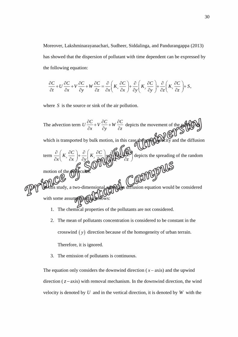
Moreover, Lakshminarayanachari, Sudheer, Siddalinga, and Pandurangappa (2013)

has showed that the dispersion of pollutant with time dependent can be expressed by

the following equation:

,x y z

C C C C C C CU V W K K K S

t x y z x x y y z z

where S is the source or sink of the air pollution.

The advection term C C C

U V Wx y z

depicts the movement of the pollutants

which is transported by bulk motion, in this case the wind velocity and the diffusion

term x y z

C C CK K K

x x y y z z

depicts the spreading of the random

motion of the molecules.

In this study, a two-dimensional advection diffusion equation would be considered

with some assumptions as follows:

1. The chemical properties of the pollutants are not considered.

2. The mean of pollutants concentration is considered to be constant in the

crosswind y direction because of the homogeneity of urban terrain.

Therefore, it is ignored.

3. The emission of pollutants is continuous.

The equation only considers the downwind direction ( x axis) and the upwind

direction ( zaxis) with removal mechanism. In the downwind direction, the wind

velocity is denoted by U and in the vertical direction, it is denoted by W with the

31

removal term denoted by C . The two dimensional advection-diffusion equation

would have the following form:

2 2

2 2,

x z

C C C C CU W K K C

t x z x z

where C is the concentration of pollutants dependent of distance in the x and z

direction as well as time t . In other words , ,C x z t is the concentration function and

its independent variables. This equation is complicated to be solved analytically and

because of this, it would be solved using numerical method to approximate the

solution.

3.2.3 Meteorological factors

As discussed earlier, meteorological factors play an important role in determining the

air quality in a particular area. Meteorological factors such as wind profile (speed and

direction), temperature, air pressure, humidity, mesoscale wind, etc. determine

pollutant concentration in a particular area. The present study would only consider

wind speed, wind direction, mesoscale wind and temperature as most of these

parameters are related. For instance, high temperature results in low humidity. Also

eddy diffusivity would be considered although it is not a meteorological factor.

Temperature affects the diffusion rate which makes it ideal for it to be considered.

The wind speed and direction determines how high or low the concentration of

pollutants would be in a particular area. Wind speed is considered to be the parameter

majorly affecting the dispersion of pollutants (Vermal and Desai, 2008).

(1)

32

When the air pollutants are emitted, they are transported horizontally by a large-scale

wind which is taken to be a function of altitude (vertical distance). Again, the

pollutants are transported both horizontally and vertically by mesoscale wind. The

large-scale wind U and the vertical diffusivity zK are parameterized as a function

of vertical height 𝑧 in the same way as shown by Lin and Hildemann (1996).

,r

r

zu u z u

z

,z z r

r

zK K z K

z

where ru u z and z z r

K K z are the measured wind speed and vertical

diffusivity at a reference height r

z and , are the constants that depend on the

atmospheric stability and surface roughness.

According to Dilley and Yen (1971), the mathematical representation of mesoscale

wind in the horizontal eu and vertical directions e

w are,

,e

r

zu ax

z

,

1e

r

az zw

z

respectively, where a is a proportionality constant.

Temperature affects the rate of dispersal of pollutants as at high temperatures,

pollutants tend to diffuse faster. In this section, a temperature formula is proposed as

33

(3)

(4)

(5)

(6)

(7)

it affects turbulence thereby affecting the mesoscale wind. The proposed temperature

formula is

2 2

2 2,

r

T T TQ

t x z

where T is the temperature, r

Q is heat diffusion.

3.2.4 Boundary and initial conditions of the advection-diffusion equation

To obtain a unique solution of the time-dependent advection-diffusion equation, the

initial and boundary conditions are needed which are appropriate to the domain.

Boundary value problems of any physical relevance have these characteristics: (1) the

conditions are imposed at two different points, (2) the solution is of interest only

between those two points, and (3) the independent variable is a space variable

(Powers, 2010). For the equation of the type:

2

2

1;

C C

x k t

0 ,0x a t

,0 ;C x f x 0 x a

0, ;C x t t

0, ;

Cx t t

x

1 0 2 0, , .

Cconst C x t const x t t

x

The condition in equation (4) is the initial value which is given at every point in the

domain of interest where f x is a given function of x alone. If 0

x is denoted as an

endpoint then the concentration at the boundary may be controlled in the same way.

(2)

34

Let t be a function of time, then the condition in equation (5) is called a Dirichlet

condition. When the flow rate is controlled by a function of time 𝛽, the condition in

equation (6) is called a Neumann condition. Another possibility of the boundary

condition is the condition in equation (7) which is called Robin condition. In this

study the zero Dirichlet boundary condition is used.

3.3 Finite Difference Method

The equation (1) is complicated to be solved analytically. One of the numerical

method for solving boundary value problems is to use finite difference methods. The

principle of finite difference methods is almost like numerical schemes used in

solving ordinary differential equations. It consists of approximating the differential

operator by replacing the derivatives in the equation using differential quotients. The

domain is partitioned in space and in time. The approximations of the solution are

computed at the space or time points.

Figure 8. Domain.

𝑐

∆𝑥

∆z

35

The domain of interest will be determined in a rectangular manner, the corner points

are , ,a b c and d as shown in Figure 8 and it is divided into subinterval with spacing

b ax

N

and

d az

N

for the spatial dimension, t for the time dimension

where N is the number of grid points and a uniform grid would be obtained. Finite

difference approximations are used to replace the derivatives using Taylor series with

the reference point at x :

1 2 32 3

2 3... ....

1! 2! 3! !

nn

n

x x x xf f f ff x x f x

x x x n x

There are three finite difference methods that can be used to find the value of

,f x x they are forward difference, backward difference and central difference.

3.3.1 Forward difference method

To find the value of a function, the independent variable is shifted forward by x ,

therefore the Taylor series expansion can be written as

1 2 32 3

2 3... ....

1! 2! 3! !

nn

n

x x x xf f f ff x x f x

x x x n x

Lets’ find the first derivative f

x

1 2 3

2 3

2 3... ....

1! 2! 3! !

nn

n

x x x xf f f ff x x f x

x x x n x

2 1

2 3

2 3... ....

2 6 !

nn

n

f x x f x x xf x f f f

x x x x n x

36

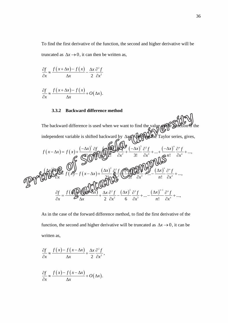
To find the first derivative of the function, the second and higher derivative will be

truncated as 0x , it can then be written as,

2

22

f x x f xf x f

x x x

.

f x x f xfO x

x x

3.3.2 Backward difference method

The backward difference is used when we want to find the value of the function if the

independent variable is shifted backward by x . Applying the Taylor series, gives,

1 2 32 3

2 3... ...,

1! 2! 3! !

nn

n

x x x xf f f ff x x f x

x x x n x

1 2 3

2 3

2 3... ...,

1! 2! 3! !

nn

n

x x x xf f f ff x f x x

x x x n x

2 12 3

2 3... ...,

2 6 !

nn

n

f x f x x x xf x f f f

x x x x n x

As in the case of the forward difference method, to find the first derivative of the

function, the second and higher derivative will be truncated as 0x , it can be

written as,

2

2,

2

f x f x xf x f

x x x

.

f x f x xfO x

x x

37

3.3.3 Central difference method

Mathematically, the central difference method is the summation of the forward

2 1

2 3

2 3... ....

2 6 !

nn

n

f x x f x x xf x f f f

x x x x n x

and the backward difference

2 1

2 3

2 3... ...,

2 6 !

nn

n

f x f x x x xf x f f f

x x x x n x

Lets’ find the first derivative f

x

2

3

3

22 ,

6

f x x f x f x f x x xf f

x x x x

2

3

3,

2 6

f x x f x x xf f

x x x

2 .

2

f x x f x xfO x

x x

This means that the central difference method has a smaller error than the other

methods.

3.3.4 The explicit finite difference scheme

The explicit method, which is also known as the Forward Time Center Space

evaluates the variable of interest at time 1n depending on the variable in the

previous time n .

38

Figure 9. Explicit finite difference scheme.

Consider the equation,

2

2;

u u

t x

0 1;x 0 ;t (8)

with boundary condition: 0, 0;u t 0 ;t

and initial condition: ,0 sin ;u x x x 0 1.x

Discretizing the domain by ,i j

x t and the value of the function u is denoted by ,.

i ju

Using the forward difference approximation for u

t

gives,

, 1 ,,

i j i ju uu

t t

and the central difference approximation for 2

2,

u

x

2

1, , 1,

2 2

2,

i j i j i ju u uu

x x

then substituting to equation (8) gives,

, 1 , 1, , 1,

2

2,

i j i j i j i j i ju u u u u

t x

1

− 1 1

39

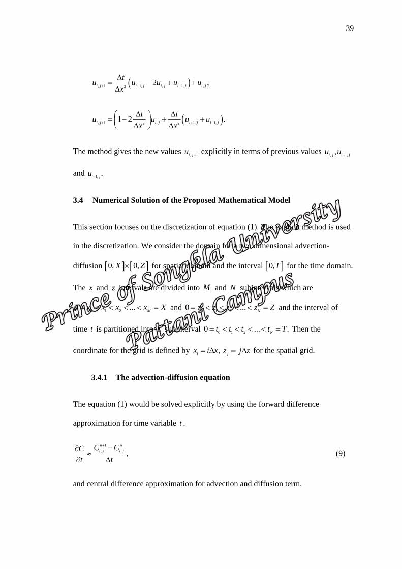
, 1 1, , 1, ,22 ,

i j i j i j i j i j

tu u u u u

x

, 1 , 1, 1,2 21 2 .

i j i j i j i j

t tu u u u

x x

The method gives the new values , 1i j

u

explicitly in terms of previous values , 1,,

i j i ju u

and 1,

.i j

u

3.4 Numerical Solution of the Proposed Mathematical Model

This section focuses on the discretization of equation (1). The explicit method is used

in the discretization. We consider the domain for a two dimensional advection-

diffusion 0, 0,X Z for spatial domain and the interval 0,T for the time domain.

The x and z intervals are divided into M and N subintervals which are

0 1 20 ...

Mx x x x X and

0 1 20 ...

Nz z z z Z and the interval of

time t is partitioned into L subinterval 0 1 2

0 ... .N

t t t t T Then the

coordinate for the grid is defined by ,i

x i x j

z j z for the spatial grid.

3.4.1 The advection-diffusion equation

The equation (1) would be solved explicitly by using the forward difference

approximation for time variable t .

1

, ,,

n n

i j i jC CC

t t

(9)

and central difference approximation for advection and diffusion term,

40

1, 1,,

2

n n

i j i jC CC

x x

(10)

, 1 , 1,

2

n n

i j i jC CC

z z

(11)

2

1, , 1,

2 2

2,

n n n

i j i j i jC C CC

x x

(12)

2

, 1 , , 1

2 2

2.

n n n

i j i j i jC C CC

z z

(13)

Substitute equation (9), (10), (11), (12) and (13) into equation (1)

1

, , 1, 1, , 1 , 1 1, , 1,

2

2

2 2

n n n n n n n n n

i j i j i j i j i j i j i j i j i j

x

C C C C C C C C CU W K

t x z x

, 1 , , 1

,2

2.

n n n

i j i j i j n

z i j

C C CK C

z

Separating the time and spatial term gives,

1

, , 1, 1, , 1 , 1 1, , 1,

2

2

2 2

n n n n n n n n n

i j i j i j i j i j i j i j i j i j

x

C C C C C C C C CU W K

t x z x

, 1 , , 1

,2

2.

n n n

i j i j i j n

z i j

C C CK C

z

Multiplying all terms by ∆𝑡 gives,

1

, , 1, 1, , 1 , 1 1, , 1,22

2 2

n n n n n n n n nx

i j i j i j i j i j i j i j i j i j

K tU t W tC C C C C C C C C

x z x

, 1 , , 1 ,22 .n n n nz

i j i j i j i j

K tC C C tC

z

Classifying each term results in,

1

, 1, 1, , 1 , 1 1, , 1,2 2 22

2 2 2 2

n n n n n n n nx x x

i j i j i j i j i j i j i j i j

K t K t K tU t U t W t W tC C C C C C C C

x x z z x x x

41

, 1 , , 1 , ,2 2 22 .n n n n nz z z

i j i j i j i j i j

K t K t K tC C C tC C

z z z

Grouping each term by the same position gives,

1

, 1, 1, , 12 2 22 2 2

n n n nx x z

i j i j i j i j

K t K t K tU t U t W tC C C C

x x x x z z

, 1 ,2 2 22 2 1 .

2

n nxz z

i j i j

K tK t K tW tC t C

z z x z

The equation above can be written as follows:

1

, 1 1, 2 1, 3 , 1 4 , 1 5 ,,n n n n n n

i j i j i j i j i j i jC AC A C AC A C A C

(14)

for 1,2,3,...,i M and 1,2,3,..., ,j N where,

1 2,

2

xK tU t

Ax x

2 2,

2

xK tU t

Ax x

3 2,

2

zK tW t

Az z

4 2,

2

zK tW t

Az z

5 2 22 2 1.x z

K t K tA t

x z

The explicit scheme will converge and be stable when 2

10 .

4

t

x

The source of emission is supposed to be 9 point grids in the middle of the domain

whereby the values come from the input from the user.

Initial concentration value ,

n

i jC is an input data from user,

42

for 1 ,..., 12 2

M Mi

and 1 ,..., 12 2

N Nj

whereby M and N must be

even number.

Boundary conditions for the concentration of pollutants are as follows:

,0 ,0,n n

i i NC C for 0,1,2,...,i M and 0,1,2,..., ,j N

0, ,0,n n

j M jC C for 0,1,2,...,i M and 0,1,2,..., .j N

3.4.2 Temperature

The equation (2) is solved in the same way as the advection-diffusion equation in

Equation (1).

1 1 1 1 1 1 1

,, , 1, , 1, , 1 , , 1

2 2

2 2.

n n n n n n n n

i j i j i j i j i j i j i j i j

r

T T T T T T T TQ

t x z

Multiplying all terms by t gives,

1 1 1 1 1 1 1

, , 1, , 1, , 1 , , 12 22 2 .n n n n n n n nr r

i j i j i j i j i j i j i j i j

Q t Q tT T T T T T T T

x z

Classifying each term gives,

1 1 1 1 1 1 1

, 1, , 1, , 1 , , 1 ,2 2 2 2 2 22 2 .n n n n n n n nr r r r r r

i j i j i j i j i j i j i j i j

Q t Q t Q t Q t Q t Q tT T T T T T T T

x x x z z z

Grouping each term by the same position,

1 1 1 1 1

, 1, 1, , 1 , 1 ,2 2 2 2 2 22 2 1 .n n n n n nr r r r r r

i j i j i j i j i j i j

Q t Q t Q t Q t Q t Q tT T T T T T

x x z z x z

(15)

43

In this work, temperature at the ground level (lower part) is different from the

temperature in the atmosphere (upper part). Hence, the temperature between them is

calculated by using linear interpolation. The following is the initial conditions of the

temperature:

1) Lower temperature (LowT): ,

n

i jT are given by input data from user for

0,1,2,...,i M and 0,1,2,3.j

2) Upper temperature (UpperT): ,

n

i jT are given by input data from user for

0,1,2,...,i M and 2, 1, ,j N N N

3) Temperature between ground level and atmosphere

,7

LowT UpperTTemperature

N

,* 3 ,n

i jT LowT Temperature j for 0,1,2,...,i M and

4,..., 3.j N

While for the boundary conditions are:

1) ,

n

i jT LowT, for 0,1,2,...,i M and 0,1,2,3,j

2) ,

n

i jT UpperT, for 0,1,2,...,i M and 2, 1, ,j N N N

3) ,* 3 ,n

i jT LowT Temperature j for 0i and 4,..., 3,j N

4) ,* 3 ,n

i jT LowT Temperature j for i M and 4,..., 3.j N

3.4.3 Parameters involved in the advection-diffusion equation

The large-scale wind, mesoscale wind and eddy diffusivity have effect on air

pollution distribution directly and temperature determines how much turbulence occur

44

which would influence the mesoscale wind, in other words temperature has an

indirect effect on air pollution distribution. Heat diffusion and air flow which is

generated by temperature would be considered as parameters in the model in equation

(15).

The large-scale wind U is a combination of the function of altitude and distance, it is

taken into account as

,,

i j r

r r

j jU u qi

z z

(16)

where r

u is the mean wind speed and q is a proportionality constant, and eddy

diffusivity

,z rj

r

jK K

z

(17)

,x ri

r

iK K

z

(18)

where r

K is the diffusivity at a reference height r

z , for the mesoscale wind W , it

would be,

,

,

min,

1 max min

n

i j

i j

r

T Taj jW b

z T T

(19)

where a is the proportionality constant and b is the air flow constant which is caused

by temperature, and all these parameters are applied for each 1,2,3...,i M and

1,2,3..., .j N

45

3.5 The Proposed Modeling of Air Pollution Distribution

This section is talk about modeling of the work we have mentioned so far. It is

enlightened from the mathematical model to the solution.

The proposed mathematical model is shown in Equation (1) as follows:

2 2

, 2 2,,

i j x zi j i j

C C C C CU W K K C

t x z x z

This model is solved explicitly by using forward time difference and central space

difference and we then obtain the discrete equation as in Equation (14); such that

1

, 1 1, 2 1, 3 , 1 4 , 1 5 ,,n n n n n n

i j i j i j i j i j i jC AC A C AC A C A C

The initial condition ,

n

i jC are given by input data from user for 1 ,..., 1

2 2

M Mi

and 1 ,..., 12 2

N Nj

, and the boundary conditions are following:

,0 ,0,n n

i i NC C for 0,1,2,...,i M and 0,1,2,..., ,j N

0, ,0,n n

j M jC C for 0,1,2,...,i M and 0,1,2,..., .j N

Simulations for the numerical solution of the advection-diffusion model would be

carried out in the next chapter. Discussion on the various figures would be shown as

well.

46

Chapter 4

Result and Discussion

This study is to analyze the distribution of pollutants under the influence of large-

scale wind, heat diffusion, air flow which is caused by temperature, mesoscale wind

and eddy diffusivity. The equations (15), (16), (17), (18), and (19) have some

unknown parameters which are , , , , , , ,r r r r

Q U z q K a b and , therefore for the

computation of air pollutants concentration, these input parameters are required. Some

of the values used in this study come from the previous study by Agarwal and Tandon

(2009), like the reference height 10r

z m and proportionality constant 10.002 .q s

The rest of the parameters have range of values as follows: 0r

Q to 25m s ,

50r

U to 50 m s , 0r

K to 25m s , a from 1 to 11s and b from 1 to 1,

these give an opportunity to test for a wider parameter value. The values of other

unknown parameters and are taken according to the stability conditions of the

atmosphere and surface roughness as shown by Irwin (1979) in table 1, with these

values of (table 1) corresponding to different stability classes, the value of can

be obtained by 1 , based on Schmidt’s conjugate power law.

Table 1. Stability and surface roughness constants.

It is assumed that pollutants are emitted at a constant rate in a uniformly distributed

Atmospheric Stability α β

Unstable 0.17 0.83

Neutral 0.27 0.73

Stable 0.61 0.39

47

domain. The area extends up to 500 m downwind and 500 m in the vertical direction.

The removal of pollutants is assumed to be taking place by either dry deposition or

wet deposition processes. The value for the removal parameter 6 110 s is assumed

to be constant in all atmospheric conditions.

An explicit finite difference scheme requires solutions to be within their range of

validity. Therefore, this analysis is done for 100M and 100N independent grid

points with each grid equal to 5 meters.

4.1 User Interface of the “Pollution Distribution Simulation” Software

In this section, the program user interface developed is shown as well as the

simulations that were carried out to study the distribution of pollutants in the

atmosphere. The various buttons are described to show how the program works and

the simulations carried out, are done by varying the atmospheric conditions and the

parameter values.

Figure 10. User interface of the program.

48

Figure 10 shows the user interface of the program used in carrying out the various

simulation of this study. The program was developed using the Lazarus programming

software. The program presents a simple user interface that is very interactive.

Figure 11. Parameter adjusting panel.

The various buttons and check boxes of the program are shown in Figure 11. This is

the part where all the parameters are adjusted in order to have a clear understanding of

how the pollutants distribute.

Figure 12. Atmospheric condition panel.

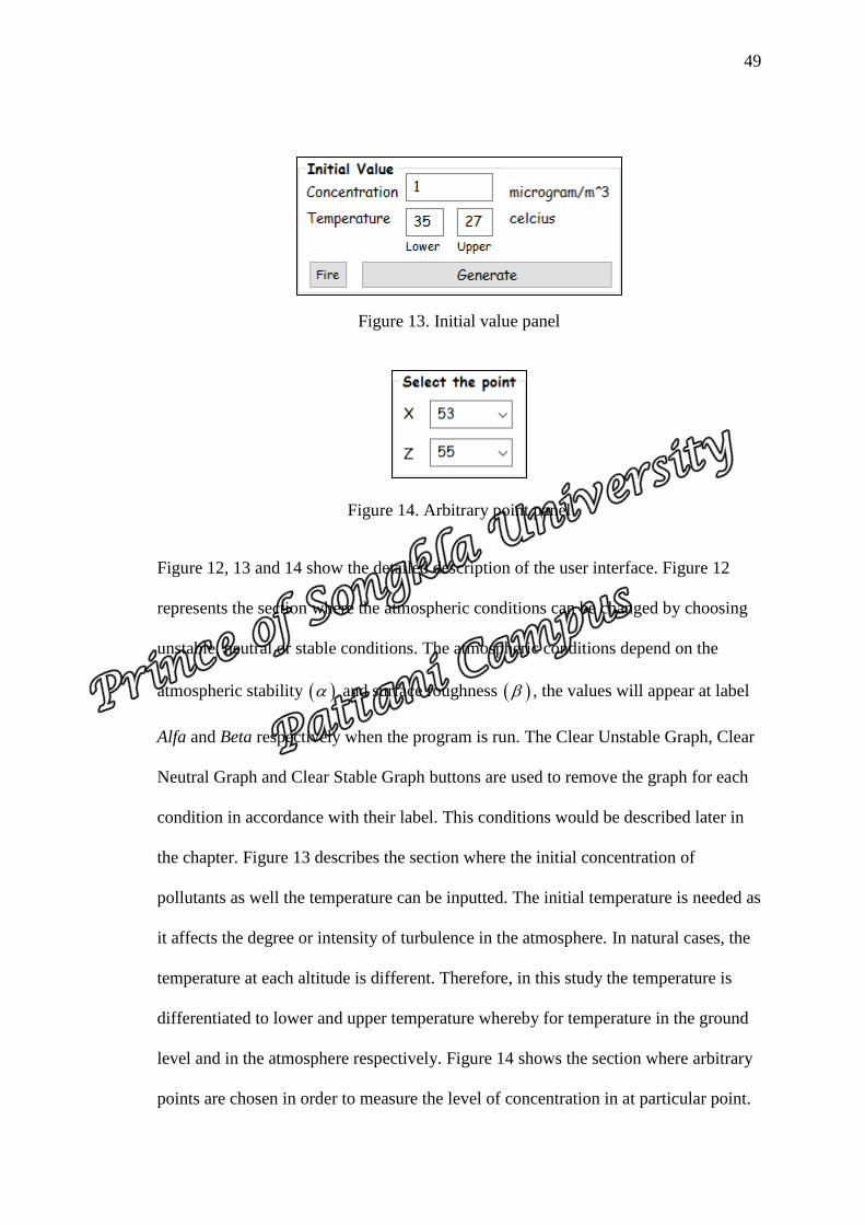
49

Figure 13. Initial value panel

Figure 14. Arbitrary point panel

Figure 12, 13 and 14 show the detailed description of the user interface. Figure 12

represents the section where the atmospheric conditions can be changed by choosing

unstable, neutral or stable conditions. The atmospheric conditions depend on the

atmospheric stability and surface roughness , the values will appear at label

Alfa and Beta respectively when the program is run. The Clear Unstable Graph, Clear

Neutral Graph and Clear Stable Graph buttons are used to remove the graph for each

condition in accordance with their label. This conditions would be described later in

the chapter. Figure 13 describes the section where the initial concentration of

pollutants as well the temperature can be inputted. The initial temperature is needed as

it affects the degree or intensity of turbulence in the atmosphere. In natural cases, the

temperature at each altitude is different. Therefore, in this study the temperature is

differentiated to lower and upper temperature whereby for temperature in the ground

level and in the atmosphere respectively. Figure 14 shows the section where arbitrary

points are chosen in order to measure the level of concentration in at particular point.

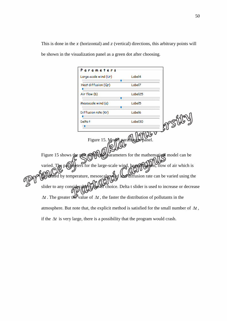
50

This is done in the 𝑥 (horizontal) and 𝑧 (vertical) directions, this arbitrary points will

be shown in the visualization panel as a green dot after choosing.

Figure 15. Model parameters panel.

Figure 15 shows the part where the parameters for the mathematical model can be

varied. The parameters for the large-scale wind, heat diffusion, flow of air which is

generated by temperature, mesoscale wind and diffusion rate can be varied using the

slider to any considerable value of choice. Delta t slider is used to increase or decrease

t . The greater the value of t , the faster the distribution of pollutants in the

atmosphere. But note that, the explicit method is satisfied for the small number of t ,

if the t is very large, there is a possibility that the program would crash.

51

Figure 16. Visualization panel.

Figure 16 shows the visualization part of the program. The yellow stack represents the

source of pollutant emission. When the program is initialized and run, pollutants are

emitted from the stack and as the model parameters are adjusted, they then distributed

in the plane. With this, the concentration can be measured when an arbitrary point is

chosen.

52

Figure 17. Graph panel.

Play Pause Stop Note Help Close

Figure 17 shows the plotting area where the concentration is plotted against time.

Figure 18 shows the various execution buttons like play, pause, stop, notes, help and

close. Each of these buttons can be used to alter the simulation process either in

running, pausing or stopping the program. The concentration values are kept in a text

file and can be viewed by pressing the note button. The change in the level of

concentration of pollutants can be viewed as a plot in Figure 17 for each of the

atmospheric conditions.

Figure 18. Execution buttons.

Time (s)

53

Figure 19. Check boxes panel.

Figure 19 shows some features of the program. Wire box check box shows the

domain in a wire form in order for the user to be able to see the grids. Axis check box

is to show the X axis and Z axis. Continuous pollution check box is to keep the

pollutant in a continuous emission. Level of concentration by color check box is to

show the level of concentration by different colors. Dynamic wind direction check

box is created in order for the mean wind speed to move dynamically by a sine

function. Draw wind, draw mesoscale wind and draw temperature check box are to

show that the magnitude of the large-scale wind, mesoscale wind and temperature

respectively are different with height.

Figure 20. Graphic value panel.

Figure 20 shows the panel to plot the graph in the different value for the same

parameter from the small value to the large value.

54

The next section shows the simulation that were carried out by the program.

4.2 Simulation

The advection-diffusion model described in chapter 3 depends on some parameters as

well as the atmospheric condition at a particular point in time. The atmospheric

condition considered are the unstable, neutral and stable which intern depend on some

constants. The constants are the atmospheric stability represented in the model as 𝛼

and the surface roughness of the earth as 𝛽 in the model (see Table 1).

To be able to gain insight clearly on air pollutants distribution under the effect of the

various model parameters like the large-scale wind, heat diffusion, air flow from the

temperature, mesoscale wind and diffusion rate simulations are carried out and then

visualized using the program developed. The program is run by choosing an

atmospheric parameter, inputting the initial concentration, temperature and the

various model parameters. Arbitrary points are then chosen and the system is

activated by clicking on the generate button (see Figure 10). The concentration of

pollutants is simulated using equation (14) and (15).

This section presents the various graphs that were plotted under the atmospheric

conditions considered in this study. Different concentration-time plots would be

shown to explain how the level of concentration of pollutants are affected by the

model parameters.

55

Figure 21. Initial value panel.

In this simulation, Figure 21 shows the initial values inputted to the program.

Figure 22. Position of the arbitrary point.

An arbitrary point is chosen by using X and Z labels in the program and the

corresponding position is shown with a green dot in the visualization panel as shown

in Figure 22.

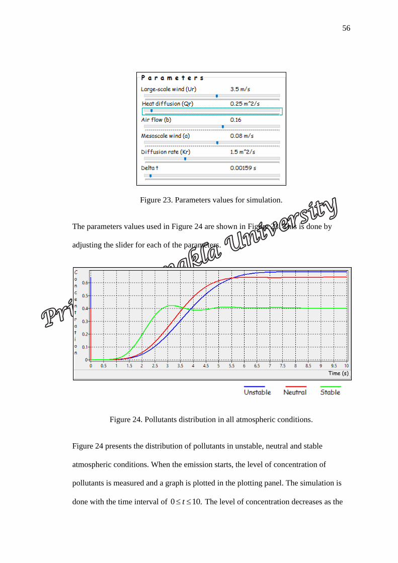
56

Figure 23. Parameters values for simulation.

The parameters values used in Figure 24 are shown in Figure 23. This is done by

adjusting the slider for each of the parameters.

Figure 24. Pollutants distribution in all atmospheric conditions.

Figure 24 presents the distribution of pollutants in unstable, neutral and stable

atmospheric conditions. When the emission starts, the level of concentration of

pollutants is measured and a graph is plotted in the plotting panel. The simulation is

done with the time interval of 0 10.t The level of concentration decreases as the

Time (s)

57

emission continuous and this can be seen in figure 22 at a 30.7 g m level under the

unstable condition, 30.64 g m under the neutral condition and

30.44 g m under

the stable condition. This is due to the difference in the atmospheric conditions as

they all have different atmospheric stability and surface roughness values. From the

graph it can be seen that at time 4.5 , 5.5 and 6 unit of time for stable, neutral and

unstable conditions respectively, the concentration of pollutants maintains some level

of constancy. This is due to the fact that, the emission is continuous and at the point

the change in concentration of the pollutants and the atmosphere is the same so there

is not any significance change. Also, the pollutants undergo an advection and

diffusion process and therefore there would always be a drop or increase in the

concentration levels in the presence of the model parameters.

Figure 25. The parameters value for simulation when the large-scale wind is

increased.

Subsequently the simulation is carried out by increasing large-scale wind to 7.5 m s

but the rest of the model parameters are maintained from the simulation was carried

out in Figure 24. The values of the parameters are shown in Figure 25.

58

Figure 26. Varying mean wind speed in all atmospheric condition.

Figure 26 shows that in each of the atmospheric conditions, the peak level of the level

of concentration of pollutants has decreased. This is evident from the previous figures

with a 30.7 g m to

30.18 g m under the unstable condition, 30.64 g m to

30.13 g m under the neutral condition and finally 30.44 g m to

30.044 g m

under the stable condition. The level of concentration of pollutants has decreased due

to an increase in the large-scale wind. This fact would be explored more later in the

chapter, as each of the parameters would be varied in one atmospheric condition. The

level of constancy in the concentration of pollutants at 6.5 , 7 and 6.8 unit of time for

the stable, neutral and unstable conditions is a result of the reasons given under the

Figure 24.

Time (s)

59

4.3 Visualizing the Effects of the Model Parameters on the Concentration of

Pollutants

The model parameters are varied and used for the unstable atmospheric condition.

This is done to see the effect they have on the distribution of pollutants in the

atmosphere. In the simulations, one particular parameter is varied whiles the others

are kept constant.

Figure 27. Pollutant distribution by varying the large-scale wind.

The simulations carried out in Figure 27 start with a large-scale wind of 7.5 𝑚/𝑠 and

this value is varied to 12.8 m s and 22.4 m s whiles the other parameters are kept

constant. Also the level of constancy in the concentration of pollutants at 8 , 7.5 and

6.5 unit of time for the small value, medium value and large value respectively in

unstable condition is as a result of the reason given under the Figure 24. Table 2

shows the model parameters and their values.

7.5m s

12.8m s

22.4m s

Time (s)

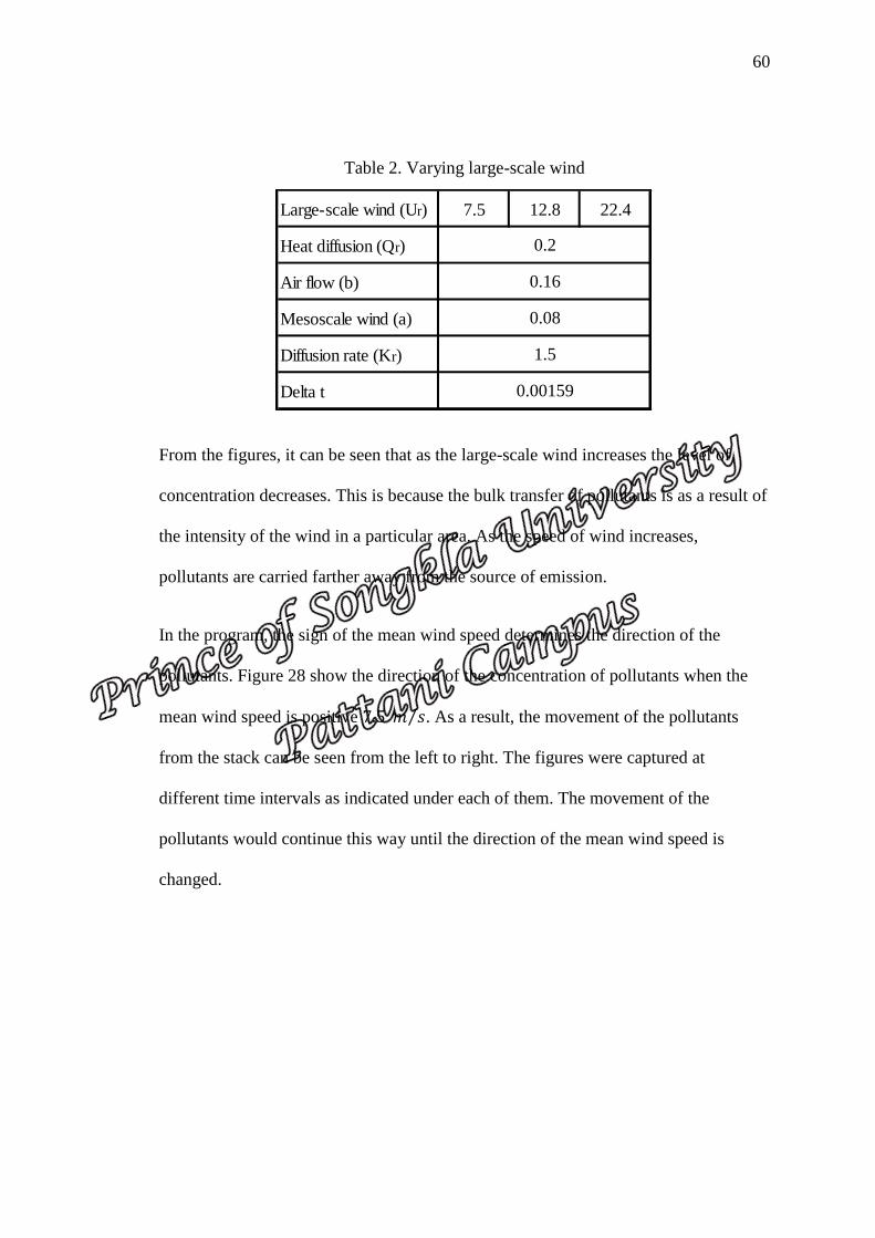
60

Table 2. Varying large-scale wind

From the figures, it can be seen that as the large-scale wind increases the level of

concentration decreases. This is because the bulk transfer of pollutants is as a result of

the intensity of the wind in a particular area. As the speed of wind increases,

pollutants are carried farther away from the source of emission.

In the program, the sign of the mean wind speed determines the direction of the

pollutants. Figure 28 show the direction of the concentration of pollutants when the

mean wind speed is positive 7.5 𝑚 𝑠⁄ . As a result, the movement of the pollutants

from the stack can be seen from the left to right. The figures were captured at

different time intervals as indicated under each of them. The movement of the

pollutants would continue this way until the direction of the mean wind speed is

changed.

Large-scale wind (Ur) 7.5 12.8 22.4

Heat diffusion (Qr)

Air flow (b)

Mesoscale wind (a)

Diffusion rate (Kr)

Delta t

0.2

0.16

0.08

1.5

0.00159

61

Figure 28. Visualization of pollutants distribution with positive large-scale wind.

As opposed to Figure 28, Figure 29 shows visualization of the emission of pollutants

from stack with a negative mean wind speed 7.5m s . The negative sign represents

the direction of the pollutants. It can therefore be seen at different time intervals the

direction of the pollutants from the right to the left and this can be changed when the

mean wind speed becomes positive.

t = 1.93303 t = 3.09496 t = 4.23087

t = 5.30379 t = 6.34072 t = 7.38364

62

Figure 29. Visualization of pollutants distribution with negative large-scale wind.

The effect of heat diffusion in the distribution of pollutants is observed with the

following simulations.

Figure 30. Pollutant distribution by varying the heat diffusion.

t = 1.86403 t = 3.07695 t = 4.24187

t = 5.34879 t = 6.41371 t = 7.50263

20.2 m s

20.5m s

23.8m s

Time (s)

63

In the transport of pollutants, advection is dominant over diffusion and therefore from

Figure 30 even though the heat diffusion is increased from 0.2 𝑚2 𝑠⁄ to 0.5 𝑚2 𝑠⁄

and then finally to 3.8 𝑚2 𝑠⁄ , there is no significant difference in the level of

concentration of pollutants. The level of constancy in the concentration of pollutants

for all values from small to large value at 8 unit of time has been explained earlier

(see Figure 24). Table 3 shows the parameter values for each of the figures.

Table 3. Varying heat diffusion rate

The air flow generated by the temperature in the atmosphere is considered as part of

the model parameters. This is a constant that is varied to see the effect it has on the

distribution of pollution.

Figure 31. Pollutant distribution by varying air flow.

Large-scale wind (Ur)

Heat diffusion (Qr) 0.2 0.5 3.8

Air flow (b)

Mesoscale wind (a)

Diffusivity (Kr)

Delta t

7.5

1.5

0.16

0.08

0.00159

0.16

0.4

0.8

Time (s)

64

From Figure 31, the level of concentration increases in the unstable atmospheric

condition as the value of air flow is increased from 0.16 to 0.4 and then 0.8.

Therefore, an increase or decrease in this value results in a corresponding increase or

decrease in the level of concentration of pollutants. In Figure 30, the level of

constancy in the concentration of pollutants for all values are the same which is at 7

unit of time. The reason is the same as explained in Figure 24. Table 4 shows the

various values for the simulation.

Table 4. Varying air flow

The temperature of the atmosphere has an effect on the turbulence and this turbulence

creates a mesoscale wind which is responsible for carrying the pollutants into the

atmosphere. The figures show that the concentration of pollutants increase when air

flow is increased.

Large-scale wind (Ur)

Heat diffusion (Qr)

Air flow (b) 0.16 0.4 0.8

Mesoscale wind (a)

Diffusivity (Kr)

Delta t

7.5

0.2

0.00159

0.08

1.5

65

Figure 32. Pollutant distribution by varying mesoscale wind.

As studied by M. Agarwal and Tandon (2009), the mesoscale wind prevents the

dispersal of pollutants which results in the increase of pollution concentration in the

atmosphere. From Figure 32, the level of concentration of pollutants increase as the

mesoscale wind is increased from 0.08 𝑚 𝑠⁄ to 0.3 𝑚 𝑠⁄ but decreased when it was

increased to 0.82 𝑚 𝑠⁄ . This is because of the position of the arbitrary point that was

chosen. The concentration of the pollutants was far from the arbitrary point and hence

a decrease in the concentration level. The other model parameters are kept constant as

the value of the mesoscale wind is varied. The level of constancy in the concentration

of pollutants at 5 , 3.5 and 3 for the small value, medium value and large value

respectively is as a result of the same reason given under Figure 24. Table 5 shows the

values used in each of the simulations carried out.

0.08m s

0.3m s

0.82m s

Time (s)

66

Table 5. Varying mesoscale wind.

The mesoscale wind is responsible for carrying the pollutants in the upwind and

downwind directions. The mesoscale wind is positive 0.3 𝑚/𝑠 and so the pollutants

would move up but the mean wind speed is positive so from Figure 33, the pollutants

move in the northeast direction at different time intervals.

Large-scale wind (Ur)

Heat diffusion (Qr)

Air flow (b)

Mesoscale wind (a) 0.08 0.3 0.82

Diffusivity (Kr)

Delta t 0.00159

7.5

0.2

0.16

1.5

67

Figure 33. Visualization of pollutants distribution with positive mesoscale wind

0.3 .m s

With a negative value of the mesoscale wind −0.3 𝑚/𝑠, the pollutants move in the

downwind direction at different times intervals as shown in Figure 34.

t = 1.99303 t = 3.33394 t = 4.65984

t = 5.91975 t = 7.16066 t = 8.42977

68

Figure 34. Visualization of pollutants distribution with positive mesoscale wind

0.3 .m s

Diffusion is the movement of molecules from a higher concentration to a lower

concentration. In this study, the higher concentration point is the source of emission

of pollutants and the lower concentration is the arbitrary point that was chosen. As the

diffusivity is increased from 0.6 𝑚2 𝑠⁄ to 1.5 𝑚2 𝑠⁄ and the finally to 3.7 𝑚2 𝑠⁄ , the

level of concentration of pollutants increase as shown in Figure 35. In this case, the

level of constancy in the concentration of pollutants at 9.5 , 6.5 and 4.5 unit of time

for the small value, medium value and large value respectively can be explained in the

same way as that of Figure 24.

t = 1.38400 t = 2.77298 t = 4.16788

t = 5.49778 t = 6.77169 t = 8.10464

69

Figure 35. Pollutant distribution by varying diffusion rate.

This due to the fact that the pollutants are diffusing at a faster rate to the arbitrary

point which tend to increase the concentration at that point. Table 6 shows the model

values that were used to carry out the simulations.

Table 6. Varying diffusivity.

Simulations for the model parameters have been carried out for each of the

atmospheric conditions and then visualized in the various figures shown. Inferences

and conclusions would be discussed in the next chapter.

The diffusivity is varied and visualized at different time intervals. This cannot be seen

clearly in movement of the pollutants from Figure 36 with diffusivity 0.6 m2/s.

Large-scale wind (Ur)

Heat diffusion (Qr)

Air flow (b)

Mesoscale wind (a)

Diffusivity (Kr) 0.6 1.5 3.7

Delta t 0.00159

0.2

0.16

0.08

7.5

20.6 m s

21.5m s

23.7 m s

Time (s)

70

Figure 36. Visualization of pollutants distribution with diffusion rate of 20.6 .m s

Figure 37 shown the movement of pollutants as the diffusivity is varied to be 3 m2/s.

This cannot be seen clearly as advection is dominant over diffusion in the transport of

pollutants in the atmosphere.

t = 1.45701 t = 2.92097 t = 4.36886

t = 5.74976 t = 7.09066 t = 8.47479

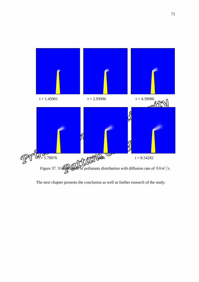
71

Figure 37. Visualization of pollutants distribution with diffusion rate of 20.6 .m s

The next chapter presents the conclusion as well as further research of the study.

t = 1.45901 t = 2.93096 t = 4.39086

t = 5.78976 t = 7.15466 t = 8.54282

72

Chapter 5

Conclusion and Further Research

5.1 Conclusion

Air pollution is one of the major atmospheric problems the world faces nowadays.

The WHO estimates millions of people dying each year as a result of pollution

problems. Dispersion models are essential in managing the ambient air quality. The

dispersion models are used to estimate the impact of the concentration of air

pollutants which have on the living organisms as well the entire ecosystem.

By using a mathematical model, it becomes easier to learn the basic concept of the

physical phenomena that takes place during the distribution of pollutants as they

undergo advection and diffusion processes under the influence of meteorological

factors. In this study, these parameters represent large-scale wind, mesoscale wind,

eddy diffusivity and temperature. These parameters have been incorporated into the

model to understand how pollutants distribute in different atmospheric stability

conditions.

The finite difference method is used to solve the model numerically. The results are

simulated and visualized using the program developed. Various simulations were

carried out in order to access how the distribution of pollutants are affected when any

of the model parameters are varied. The large-scale wind shows a significant change

in the level of concentration of pollutants. The increase or decrease in the large-scale

wind resulted in a corresponding increase or decrease in the level of concentration of

pollutants. The mesoscale wind however showed different results. An increase in the

73

mesoscale wind resulted in an increase in the concentration levels. Therefore, the

transport of pollutants from the source of emission depends largely on the large-scale

wind as advection is dominant over diffusion in this process.

Through the various simulations, the effect of the parameters on the distribution of

pollutants can be appreciated as it makes it easier to understand the pollution

distribution concept. Although the concentration of pollutants cannot be reduced after

it has been released into the atmosphere, but through this study, the government and

other stake holders can be advised in order to make policies that would cut down the

production of 2,

sNO SO and other harmful pollutants through coal power plants by

going green. That is encouraging the use of renewable energy. The visualization of

the pollutants can be used to explain the pollution problems to communities on how

meteorological parameters affect the distribution of pollutants.

5.2 Further research

The entire study of pollutants distribution is largely based on simulations but in

further research, real meteorological data can be used to confirm the validity of the

model. Again, some removal mechanisms can be added to the simulation in order to

know the actual concentration of pollutants after these physical processes.

74

References

Agarwal, M. and Tandon, A. 2009. Modeling of the urban heat island in the form of

mesoscale wind and of its effect on air pollution dispersal. Applied

Mathematical Modelling. 34, 2520-2530.

Alloway, B. J. and Ayres, D. C. 1993. Chemical Principles of Environmental

Pollution. Glasgow: Blackie Academic & Professional, an Imprint of Chapman

& Hall, pp. 16, 25.

Arystanbekova, N. Kh. 2004. Application of Gaussian plume models for air

pollution simulation at instantaneous emissions. Mathematics and Computers in

Simulation. 67, 451-458.

Awasthi, S., Khare, M. and Gargava, P. 2006. General plume dispersion model

(GPDM) for point source emission. Environmental Modeling and Assessment.

11, 267-276.

Bell, J.N.B. and Treshow, M. 2002. Air pollution and plant life, 2nd ed. John Wiley

& Sons, Ltd. West Sussex, England.

Dilley, J.F. and Yen, K.T. 1971. Effect of a mesoscale type wind on the pollutant

distribution from a line source. Atmospheric Environment. 5, 843-851.

Duki. M. I. Z., Sudarmadi. S., Suzuki. S., Kawada. T., and Tri-Tugaswati. A. 2010.

Effect of air pollution on respiratory health in Indonesia and its economic cost.

Environmental Health. 58, 135-143.

75

Fenger. J., and Tjell. J. C. 2009. Air pollution from a local to a global perspective.

Polyteknisk Forlag, Denmark, pp. 293.

Hosseinibalam, F. and Hejazi, A. 2012. Influence of meteorological parameters on

air pollution in Isfahan. 3rd International Conference on Biology, Environment

and Chemistry, 2012, 46.

Irwin, J. S. 1979. Technical note: A theoretic variation of the wind profile power law

exponent as a function of surface roughness and stability. Atmospheric

Environment. 13, 191-194.

Jakeman. A. J. Beck. M. B. and McAlee. M. J. 1995. Modelling change in

environmental systems. John Wiley & Sons Ltd, England, pp. 317.

Lakshminarayanachari. K. Sudheer, P. K. L. Siddalinga, P. M. and Pandurangappa, C.

2013. Advection – diffusion numerical model of air pollutants emitted from an

urban area source with removal mechanisms by considering point source on the

boundary. International journal of Application or Innovation in Engineering and

Management. 2, 251-268.

Lakshminarayanachari. K. Suresha, C. M. Siddalinga, M. P. and Pandurangappa, C.

2013. Numerical model of air pollutant emitted from an area source of primary

and secondary pollutants with chemical reaction and gravitational settling with

point source on the boundary. International Journal of Research in

Environmental Science and Technology. 3(1), 9-18.

76

Lin, J.S. and Hildemann, L.M. 1996. Analytical solutions of the atmospheric

diffusion equation with multiple sources and height dependent wind speed and

eddy diffusivities. Atmospheric Environment. 30, 239-254.

Nevers, N.D. 2000. Air pollution control engineering. 2nd ed. McGraw-Hill,

Singapore, pp. 1, 119.

Pandurangappa, C. Lakshminarayanachari, K. and Venkatachalappa, M. 2012. Effect

of mesoscale wind on the pollutant emitted from an area source of primary and

secondary pollutants with gravitational settling velocity. International Journal of

Emerging Technology and Advanced Engineering. 2(9), 325-334.

Powers. D. L. 2010. Boundary value problems and partial differential equations. 6th

ed. Academic Press, USA, pp. 25.

Ramaswami, A. Milford, J. B. and Smal, M. J. 2005. Integrated environmental

modeling: pollutant transport, fate, and risk in the environment. John Wiley &

Sons, Inc, Canada, pp. 10.

Sudheer, P K. L., Lashminarayanachari, K., Prasad, M. S., and Pandurangappa, C.

2012. Numerical model of air pollutant emitted from an area source of primary

and secondary pollutants with chemical reaction and dry deposition.

International Journal of Science, Environment and Technology. 1, 1-14.

Suresha, C. M., Lakshminarayanachari, K., Prasad, M. S. and Pandurangappa, C.

2013. Numerical model of air pollutant emitted from an area source of primary

pollutant with chemical reaction. International Journal of Application or

Innovation in Engineering and Management. 2(3), 132 – 144.

77

Venkatachalappa, M., Khan, S. K. and Kakamari, K. A. G. 2003. Time dependent

mathematical model of air pollution due to area source with variable wind

velocity and eddy diffusivity and chemical reaction, in Proc. Indian Natn Sci

Acad 69, A, No. 6, 2003, 745-758.

Verma, S. S., and Desai, B. 2008. Effect of meteorological conditions on air

pollution of Surat city. J. Int. Environmental Application & Science, 3(5), 358-

367.

ELECTRONIC REFERENCES

Eberhard, K. 2016. Why Oregon Needs the Healthy Climate Act. Available online:

http://www.sightline.org/2016/02/16/why-oregon-needs-the-healthy-climate-

act/, [May 2, 2016].

EPA. Air Pollution: Current and Future Challenges. Available online:

https://www.epa.gov/clean-air-act-overview/air-pollution-current-and-future-

challenges, [May 2, 2016].

2006. How Convection and Advection Moves Pollution. Available online:

http://astro.hopkinsschools.org/course_documents/earth_moon/earth/earth_scien

ce/convection/pollution_transfer.htm, [Dec 13, 2015].

NC State University. 2012. Stability. Available online:

http://climate.ncsu.edu/edu/k12/.Stability, [July 25, 2016].

The Jakarta Post. 2015. Asean Help Needed on Smog, Says Thai PM. Available

online: http://www.thejakartapost.com/news/2015/10/07/asean-help-needed-

smog-says-thai-pm.html, [Dec 13, 2015].

78

Wencong, W. 2013. State Council Gives Approval to Tough Air Emissions Plan.

Available online: http://usa.chinadaily.com.cn/epaper/2013-

07/25/content_16829757.htm, [May 2, 2016].

Wikipedia. Raung. Available online: https://en.wikipedia.org/wiki/Raung, [Dec 13,

2015].

World Health Organization. 2016. Air Pollution. Available online:

http://www.who.int/topics/air_pollution/en/, [May 1, 2016].

World Health Organization. 7 Million Premature Deaths Annually Linked to Air

Pollution. Available online:

http://www.who.int/mediacentre/news/releases/2014/air-pollution/en/, [Jan 20,

2015].

79

APPENDIX

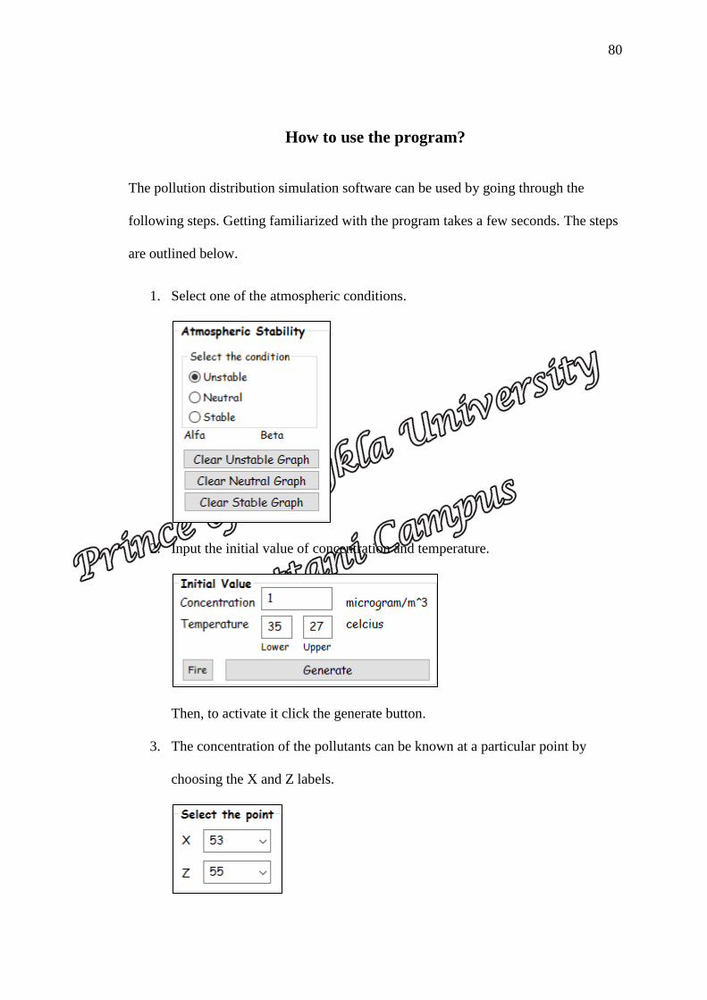
80

How to use the program?

The pollution distribution simulation software can be used by going through the

following steps. Getting familiarized with the program takes a few seconds. The steps

are outlined below.

1. Select one of the atmospheric conditions.

2. Input the initial value of concentration and temperature.

Then, to activate it click the generate button.

3. The concentration of the pollutants can be known at a particular point by

choosing the X and Z labels.

81

4. The mean wind speed, heat diffusion, flow from the temperature, turbulence,

diffusion rate can be varied by using the slider.

5. Click the play button to run the program, button to pause the

program, button to stop the program, button to save the

concentration value of pollutants in a file, button to as a guide in using

the program and button to close the program.

82

Algorithm of the program

Var {variables for the model}

{the variables for the model are defined in order to be used in the various procedure}

Const WD = 100 {the number of grid horizontally}

Const HD = 100 {the number of grid vertically}

Const zr = 10 {reference height}

Const IVC = 1 {initial value of concentration}

Const IVT = 27 {initial value of temperature}

{defining the data types for the variables}

Time : single

dt : single

dh : single

Lamda : single

Ur : real

a : real

Kr : real

Qr : real

alfa, beta : real

b : real

{creating an array}

wind : array [1..WD, 1..HD] of single

we : array [1..WD, 1..HD] of real

Kx, Kz : array [1..HD] of real

Tnew, Tnow : array [0..WD, 0..HD] of single

Cnew, Cnow : array [0..WD, 0..HD] of single

Algorithm

{simulation}

Procedure 1.

{in this procedure, the initial values are set for subsequent calculation in the program}

begin

Ur 0.01

a 0.01

Kr 0.01

Qr 0.0007

83

b 0.01

Time 0 {initial computational time}

dt 0.001 {time increment}

dh 5 {spatial increment dx = dz = dh}

Lamda 0.000001

for j 0 to HD do

for i 0 to WD do

begin

Tnow [i,j] IVT

end

end procedure.

Procedure 2.

{in order to run the program, the various atmospheric parameters are enabled. This is

done by using a check box}

read (radiogroup)

if unstable.checked then

alfa 0.17

beta 0.83

end if

if neutral.checked then

alfa 0.27

beta 0.73

end if

if stable.checked then

alfa 0.61

beta 0.39

end if

{this section calculates the various parameters for the model using the formula from

the model}

for j 1 to HD-1 do

begin

Kz [j] 𝐾𝑟 (𝑗

𝑧𝑟)𝛽

for i 1 to WD-1 do

begin

Kx [i] 𝐾𝑟 (𝑖

𝑧𝑟)𝛽

84

Wind [i,j] 𝑢𝑟 (𝑗

𝑧𝑟)𝛼

(𝑗

𝑧𝑟)𝛼

Tnew [i,j] 𝑄𝑟 ∆𝑡

∆𝑥2𝑇𝑖+1,𝑗𝑛−1

𝑄𝑟 ∆𝑡

∆𝑥2𝑇𝑖−1,𝑗𝑛−1

𝑄𝑟 ∆𝑡

∆𝑧2𝑇𝑖,𝑗+1𝑛−1

𝑄𝑟 ∆𝑡

∆𝑧2𝑇𝑖,𝑗−1𝑛−1

(−2𝑄𝑟 ∆𝑡

∆𝑥2− 2

𝑄𝑟 ∆𝑡

∆𝑧2𝑇𝑖,𝑗𝑛−1 1)𝑇𝑖,𝑗

𝑛−1

we [i,j] 𝑎 𝑗

(𝛼+1)(𝑗

𝑧𝑟)𝛼

(𝑇𝑖,𝑗𝑛−𝑚𝑖𝑛𝑇𝑖,𝑗

𝑛

𝑚𝑎𝑥𝑇𝑖,𝑗𝑛−𝑚𝑖𝑛𝑇𝑖,𝑗

𝑛)

end

end

end procedure.

Procedure 3.

{the initial concentration is inputted in this procedure and procedure 2 is called to use

the atmospheric condition. Procedure 5 is then used in order to draw the

corresponding graphs}

Call procedure 2

Call procedure 5

{input the initial concentration}

Cnow [50,50] IVP

Cnow [49,50] IVP

Cnow [49,51] IVP

Cnow [51,50] IVP

Cnow [51,51] IVP

Cnow [50,49] IVP

Cnow [49,49] IVP

Cnow [50,51] IVP

Cnow [51,49] IVP

{calculating concentration with the concentration formula}

for j 1 to HD-1 do

begin

for i 1 to WD-1 do

begin

Cnew [i,j] 𝐴1𝐶𝑖+1,𝑗𝑛 𝐴2𝐶𝑖−1,𝑗

𝑛 𝐴3𝐶𝑖,𝑗+1𝑛 𝐴4𝐶𝑖,𝑗−1

𝑛 𝐴5𝐶𝑖,𝑗𝑛 .

end

end

end procedure.

Procedure 4.

85

{activate the initial value}

Call procedure 1.

Call procedure 2.

{setting the selected point to measure the concentration of pollutant using the combo

box}

for i 0 to WD do {for setting point X}

begin

Combobox1 [i] 0 … 100

end

for j 0 to HD do {for setting point Z}

begin

Combobox2 [j] 0 … 100

end

{visualization}

Procedure 5.

{in this procedure, the graph for the three atmospheric condition can be drawn for

visualization}

begin

if Unstable.Checked then

begin

UnstableSeries1.

end;

if Neutral.Checked then

begin

NeutralSeries1.

end;

if Stable.Checked then

begin

StableSeries1.

end;

end;

Procedure 6.

{this procedure use openGL utility to draw the image for visualization}

Var {local variable for procedure 6 only}

Speed : double

86

DataRange : double

begin

glClearColor(0.0, 0.0, 0.0, 1.0);

glClear(GL_COLOR_BUFFER_BIT or GL_DEPTH_BUFFER_BIT);

glEnable(GL_DEPTH_TEST);

glMatrixMode(GL_PROJECTION);

glLoadIdentity();

gluPerspective(45.0, double(Width) / height, 0.2, 100.0);

glMatrixMode(GL_MODELVIEW);

glLoadIdentity();

glTranslatef(-1.0, 0.0,-3.0);

glTranslatef(Tran_X,Tran_Y,Tran_Z);

glRotatef(alpha+dx,0.0,1.0,0.0);

glRotatef(betha+dy,1.0,0.0,0.0);

if Axis.Checked then

begin

glBegin(GL_LINES);

glColor3f(1.0,0.0,0.0);

glVertex3f(-1.0,0.0,0.0);

glVertex3f( 1.0,0.0,0.0);

glColor3f(0.0,1.0,0.0);

glVertex3f(0.0,-1.0,0.0);

glVertex3f(0.0, 1.0,0.0);

glColor3f(0.0,0.0,1.0);

glVertex3f(0.0,0.0,-1.0);

glVertex3f(0.0,0.0, 1.0);

glEnd();

end;

if (MaxC-MinC) = 0 then

begin

MaxC 1;

MinC 0;

end;

if WireBox.Checked then

begin

glPolygonMode(GL_FRONT_AND_BACK,GL_LINE) {to show grid}

end else

begin

87

glPolygonMode(GL_FRONT_AND_BACK,GL_FILL); {to show plane}

end;

DataRange MaxC-MinC;

{drawing source of emission}

glPointSize(7); { size of the point }

glBegin(GL_POINTS);

glcolor3f(0,1,0);

glPointSize(10);

glvertex3f(-1+(PointX)*(4/WD), -1+PointZ*(2/HD), 0.01);

glpointsize(1);

glEnd();

{drawing the stack}

glBegin(GL_POLYGON);

glColor3f(1.0,1.0,0);

glvertex3f(-1+((WD div 2)-5)*(4/WD), -1+(1)*(2/HD), 0.01);

glvertex3f(-1+((WD div 2)-2)*(4/WD), -1+((HD div 2)-1)*(2/HD), 0.01);

glvertex3f(-1+((WD div 2)+2)*(4/WD), -1+((HD div 2)-1)*(2/HD), 0.01);

glvertex3f(-1+((WD div 2)+5)*(4/WD), -1+(1)*(2/HD), 0.01);

glEnd();

{configurating the 4 boundary condition}

{North}

for j 0 to 0 do

for i 0 to WD do

begin

Cnow[i,j] Cnow[i,j+1];

end;

{South}

for j HD to HD do

for i 0 to WD do

begin

Cnow[i,j] Cnow[i,j-1];

end;

{West}

for j 0 to HD do

for i 0 to 0 do

88

begin

Cnow[i,j] Cnow[i+1,j];

end;

{East}

for j 0 to HD do

for i WD to WD do

begin

Cnow[i,j] Cnow[i-1,j];

end;

{tranfer the Cnew to Cnow and Tnew to Tnow}

for j 1 to HD-1 do

for i 1 to WD-1 do

begin

Cnow[i,j] Cnew[i,j];

Tnow[i,j] Tnew[i,j];

end;

Speed := double(OpenGLControl1.FrameDiffTimeInMSecs)/10;

cube_rotationx += 5.15 * Speed;

cube_rotationy += 5.15 * Speed;

cube_rotationz += 20.0 * Speed;

Time Time + dt;

{finalize with swap buffer / refresh openGL}

OpenGLControl1.SwapBuffers;

end;

Procedure 7.

{to call procedure 3 and procedure 6}

Call procedure 3.

Call procedure 6.

Procedure 8.

{to run the program}

begin

MaxC := 0;

MinC := 0;

89

Ur := TrackBar1.Position/100; {The Mean Wind Speed (Ur)}

a := TrackBar2.Position/100; {Turbulence (a = proportionality constant)}

Kr := TrackBar3.Position/100; {Diffusion Rate (Kx / Kz)}

Qr := TrackBar4.Position/100; {Heat Diffusion (Qx / Qz)}

b := TrackBar5.Position/100; {b = the flow caused by the temperature}

call procedure 2.

Timer1.Enabled := True;

end;

90

Vitae

Name : Syafika Ulfah

Student ID : 5620320706

Educational Attainment:

Degree Name of Institution Year

B. Sc. (Mathematics Education) Univ. Muhammadiyah Prof. Dr. Hamka 2012

Scholarship Awards during Enrolment

SAT Scholarship for International Student of Faculty of Science and Technology,

Faculty of Science and Technology, Prince of Songkla University.

International Conference

Ulfah, S. and Chuai-Aree, S. Modeling, Simulation and Visualization of Air Pollution

Distribution Using an Advection-Diffusion Model. Annual Int’l Conference on

Intelligent, Computer Science & Information Systems (ICCSIS-16) April 28-29, 2016

Pattaya (Thailand).