Embed Size (px)
Citation preview

Measurements and numerical simulations of1
the activation degree and vegetation cover on2
parabolic dunes in north-eastern Brazil3
O. Duran a,∗ M.V.N. Silva b L.J.C. Bezerra c H.J. Herrmann d,e4
L.P. Maia c5
aInstitute for Computational Physics, Universitat Stuttgart, Pfaffenwaldring 27,6
D-70569 Stuttgart, Germany7
bUniversidade Federal do Pernambuco, Dept. Geos., Moraes Rego 1235, CEP8
50670-901, Recife, Brazil9
cUniversidade Federal Ceara, Dept. Geol., Campus Pici Bloco 912, BR-6045597010
Fortaleza, Ceara, Brazil11
dComputational Physics, IfB, HIF E12, ETH Honggerberg, CH-8093 Zurich,12
Switzerland13
eDepartamento de Fısica, Universidade Federal do Ceara, 60451-970 Fortaleza,14
Ceara, Brazil15
Abstract16
In this work we present measurements of vegetation cover over parabolic dunes with17
different degree of activation along the north-eastern Brazilian coast. We extend18
the local values of the vegetation cover density to the whole dune by correlating19
measurements with the relative brightness index C of high resolution QuickBird20
panchromatic satellite image of the dune field. Next, we introduce the vegetation21
data into a continuous model for vegetated dunes, coupling sand erosion and vegeta-22
tion growth, and perform simulations of parabolic dunes. Finally, from the compar-23
ison of both, the measurements and the simulation results, we show that the model24
is able to predict the dune shape and the vegetation distribution of real parabolic25
dunes as result of the evolution of a blow-out.26
Key words: coastal morphology, vegetation cover, parabolic dunes, dune dynamics27
∗ Corresponding author. Permanent address: Multi Scale Mechanics (MSM), TS,Twente University, P.O.Box 217, 7500 AE Enschede, Netherlands. Tel.: +31 53 4892694.
Email address: [email protected] (O. Duran ).
Preprint submitted to Elsevier 22 March 2008
Manuscript

1 Introduction28
The problems posed by dune mobility have been solved in practice using differ-29
ent techniques. Small dunes can be mechanically flattened so that sand moves30
as individual grains rather than as a single body. However, such methods are31
too expensive for large dunes. These can be immobilized by covering them32
with oil or by the erection of fences. These solutions have the drawback of not33
providing long term protection since the sand remains exposed. To overcome34
this shortcoming, a suitable solution is to vegetate the sand covered areas in35
order to prevent sediment transport and erosion (Pye and Tsoar, 1990). This36
method is particularly important for coastal management where a strong sand37
transport coexists with favorable conditions for vegetation growth.38
The stabilization of mobile sand using vegetation is a well established tech-39
nique. This method has been used with excellent results on coastal dunes in40
Algeria, Tunisia, North America, United Kingdom, Western Europe, South41
Africa, Israel among others (Pye and Tsoar, 1990). Vegetation growth leads42
to stabilize sand dunes (Hack, 1941; Pye, 1982; Anthonsen et al., 1996; Muck-43
ersie and Shepherd, 1995; Hesp, 1996), preventing sand motion (Lancaster and44
Baas, 1998) and stimulating soil recovery (Tsoar, 1990; Danin, 1991).45
Recently, we developed a mathematical description of the relationship between46
vegetation growth and sand transport (Duran and Herrmann, 2006). This47
model is able to predict the stabilization of barchan dunes driven by vegetation48
growth, and, in particular, their transformation into parabolic dunes. Since49
numerical simulations are orders of magnitude faster than the real evolution,50
we are able to study the entire stabilization process and to forecast thousands51
of years of real evolution.52
Parabolic dunes are vegetated dunes that, when active, migrate along the53
prevailing wind direction. They arise under uni-directional wind and in places54
partially covered by plants and have a typical U shape with the ‘nose’ pointing55
downwind and the two arms pointing upwind, in contrast to barchan dunes56
where the horns point downwind (Fig. 1) (Pye, 1982; Tsoar and Blumberg,57
2002). Vegetation covers most of the arms of parabolic dunes and a fraction58
of their nose depending on the activation degree of the dune, i.e. how fast59
the dune moves. An active parabolic dune has a sandy nose (Fig. 1, left)60
while an inactive one is almost totally covered by plants (Fig. 1, right). Plants61
typically grow along the lee size of the dune, including the dune’s flanks,62
which are protected from wind erosion. In contrast, the interior side exposed63
to the wind is devoid of vegetation. There, erosion is strong enough to prevent64
vegetation growth.65
(Position of Fig. 1)66
2

Migrating velocity of parabolic dunes is several times smaller than that of67
barchan dunes, and in general, they are in an intermediate state between fully68
active crescent dunes, like barchans, and completely stabilized fossil dunes.69
The activation degree of parabolic dunes can be well characterized by the70
vegetation cover pattern over it, which gives information about the areas of71
sand erosion and deposition pattern responsible for the motion of the dune.72
The dynamics of parabolic dunes and their response to external perturbations,73
such as climatic change and human interference, has been the subject of several74
field works (Anthonsen et al., 1996; Tsoar and Blumberg, 2002; Arens et al.,75
2004). Here we study the activation degree of parabolic dunes in north-eastern76
Brazil by direct measurement of the vegetation cover on them. We further77
present a method to extend the local information about vegetation cover to78
the whole dune by comparing the measured vegetation density cover with the79
relative brightness index C of high resolution QuickBird panchromatic satellite80
images. The empirical vegetation cover is finally quantitatively compared to81
the numerical solution of an established model for sand transport coupled with82
vegetation growth.83
2 Regional setting84
In several sections of the coast of the province of Ceara in the north-east of85
Brazil (Fig. 2), sand dunes are totally or partially stabilized by vegetation. On86
one hand, the humid climate of the region, with intense precipitation during87
the rainy season from February to July (up to 700 mm/month and an annual88
average of more than 100 mm, see Fig. 3a), amplifies the role of vegetation89
as an active agent in the sandy landscape evolution. On the other hand, the90
ubiquity of sandy beaches combined with a strong and highly uni-directional91
ESE coastal wind (Fig. 3b), creates favorable conditions for the evolution of92
crescent sand dunes.93
(Position of Figs. 2 and 3)94
Furthermore, the wind is very strong during the dry season (July-December,95
Fig. 3), while it lays below the sand transport threshold during the rainy96
season (January-June), when the biomass production is highest. This out-97
of-face seasonal timing enhances the competing dynamics of both processes,98
the surface erosion due to sand transport and vegetation growth, which similar99
timescales of the order of months. As a results, after years of evolution, crescent100
dunes are often stabilized and parabolic dunes actually dominate the coastal101
landscape.102
In order to obtain information about the distribution of vegetation over coastal103
3
dunes, we went to Fortaleza during the rain season to measure the shape of104
some parabolic dunes and the vegetation that covers them (Fig. 4). These105
dunes are located in Iguape, on the east of Fortaleza, and Pecem, Taiba and106
Paracuru, on the west (Fig.2). The geographical coordinates of all points are107
recorded with GPS and inserted in the digital dune map.108
By using QuickBird satellite images with a resolution of 0.6m/pixel and a109
topographic map we were able to select parabolic dunes with different activity110
degrees and vegetation cover density. Figures 4a, b, c, and d, show, in order111
of activity, the four measured parabolic dunes on the west coast of Fortaleza,112
while Figs. 4e, f, and g, show the other three dunes from the Iguape region,113
on the east coast. In general, the most active ones were located in Taiba114
and Iguape (shown in Figs. 4d and g, respectively), while those in Paracuru115
(Figs. 4a and b) were among the most inactive ones.116
(Position of Fig. 4)117
3 Methods118
Since plants locally slow down the wind they can inhibit sand erosion as well119
as enhance sand accretion, as it is shown in Fig. 5 (Wolf and Nickling, 1993).120
This dynamical effect exerted by plants on the wind, which is characterized by121
the drag force acting on them, is mainly determined by the frontal area density122
λ ≡ Af/A, where Af is the total plant frontal area, i.e. the area facing the123
wind, of vegetation placed over a given sampling area A (Musick and Gillette,124
1990; Stockton and Gillette, 1990). Furthermore, the vegetation cover over a125
dune is defined by the basal area density ρv ≡ Ab/A, where Ab is the total126
plant basal area, i.e. the area covering the soil, on A (Raupach et al., 1993).127
(Position of Fig. 5)128
The distinction between both densities is crucial for the modeling of the veg-129
etation effect over wind strength and thus sand transport (Raupach, 1992;130
Raupach et al., 1993). From Fig. 5 it is clear that plants act as obstacles that131
absorb part of the momentum transferred to the soil by the wind. As a re-132
sult, the total surface shear stress τ can be divided into two components, a133
shear stress τv acting on the vegetation and a shear stress τs acting on the134
sand grains. When plants are randomly distributed and the effective shelter135
area for one plant (see Fig. 5) is proportional to its frontal area, the absorbed136
shear stress τv is proportional to the vegetation frontal area density λ times137
the undisturbed shear τs. Using this two assumptions, Raupach (1992), and138
later Raupach et al. (1993), has proposed a model for the fraction of the total139
stress acting on sand grains, which is given by140
4

τs =τ
(1−mρv)(1 + mβλ)(1)
where β is the ratio of plant to surface drag coefficients and the constant m is141
a model parameter that accounts for the non-uniformity of the surface shear142
stress (Raupach et al., 1993; Wyatt and Nickling, 1997). The term (1−mρv)143
arises from the relation between the sandy and the total area.144
Measurements on shear stress partitioning in real conditions and controlled145
wind tunnel experiments (Musick and Gillette, 1990; Wyatt and Nickling,146
1997; King et al., 2005, 2006; Gillies et al., 2007) have found reasonable agree-147
ment with the Raupach et al. (1993) model.148
Although ρv and λ can be calculated from direct measurements of the plants, in149
order to estimate the parameters β and m in Eq. 1 we need a far more complex150
procedure since in this case we have to measure the drag forces acting on the151
plants and the shear stresses on the sand surface with and without plants152
(Wyatt and Nickling, 1997; King et al., 2006; Gillies et al., 2007). We visited153
the field location during the rainy season when winds are exceptionally weak.154
The vegetation cover over any of the measured dunes includes at least six155
different species. We focused on measuring the static quantities like densities,156
rather than the dynamic ones like β and m. In the section regarding the157
numerical solution of the model we use reported values from the literature for158
these two parameters (Wyatt and Nickling, 1997).159
The basal and frontal area density, ρv and λ, can be indirectly estimated from160
the local number ni, basal area abi and frontal area afi of each species i of161
plants over a characteristic area A on the dune162
ρv ≡Ab
A=
1
A
∑i
niabi (2)
λ≡ Af
A=
1
A
∑i
niafi (3)
Figure 6 shows an sketch illustrating the local basal ab and frontal area af of163
a given plant.164
(Position of Figs. 6 and 7)165
In order to measure the basal and frontal vegetation area density over the166
dunes shown in Fig. 4, which are mainly covered by grass, we select five to ten167
points along the longitudinal and transversal main axes of the parabolic dune168
(red dots in Fig. 4). On every point we identify each plant i the number of169
times ni it appears in a study area A = 1 m2 and measure their characteristic170
length, height, number of leafs and leaf area (Fig. 7, left). Some species of the171
5

Table 1Vegetation morphology data. Lengths are in cm and areas in cm2.
Name L l h a b n ab af
Cyperus maritimus (CM) – – 5 0.8 10 5–6 24 12
Remirea maritima (RM) – 2 8 – – – 3 6
Heliotropium polyphyllum (HP) 20 10 8 0.8 – 3–4 29 19
Chamaecrista hispidula (CH) 25 10 2 3 2 5 120 60
Ipomoema pes-caprae (IP) 100 10 15 8 9 6 500 83
Turnera subulata (TS) – – – 2 2 12 48 24
Sporobolus virginicus (SV) – – – 0.2 1-4 12 3 3L total length for elongated plantsl characteristic length of the branchesh characteristic plant heighta leaf width or characteristic branch widthb leaf lengthn number of leafs or branchesab plant effective basal areaaf frontal plant area
typical vegetation we found are shown on the right side of Fig. 7. Using the172
morphological information of each species i (table 1) we measure the fraction173
of the total leaf area of each plant that covers the soil abi, and the fraction174
that faces the wind afi. From Eq. 2, it is then possible to calculate the basal175
and frontal are density at each study point (table 2).176
In general, we found the same qualitative distribution of plants on all measured177
parabolic dunes (Fig. 8 and table 2). The area between the arms of the dune178
is totally covered by plants, i.e. ρv > 20% (Levin et al., 2007), while their179
density decreases on the windward side where sand erosion is very strong and180
increases once again on the lee side, where most of the sand deposition occurs.181
(Position of Fig. 8)182
4 Model for vegetated dunes183
The numerical study of parabolic dunes has recently experienced new devel-184
opments based on cellular automaton models (Nishimori and Tanaka, 2001;185
Baas, 2002; Baas and Nield, 2007). Furthermore, we have recently proposed186
a continuum approach for the study of the competition process between veg-187
etation growth and sand erosion (Duran and Herrmann, 2006).188
6

Table 2Example of the frequency of plants (given by their initials) and resulting basal coverρv in the study areas on a typical measured parabolic dune shown in Fig. 8. Thenumber of the study area correspond to the location in Fig. 8.
Number HP CH IP TS SV ρv%
1 3 – 1 1 – 6.3
2 7 – – 22 15 2.5
3 35 – – – 114 1.4
4 2 – – – 84 3.4
5 – – – – 744 24.8
6 – – – 5 504 19.2
7 34 – – 1 105 4.0
8 34 – – – – 9.8
9 23* – – – – 2.2
10 4 14 – – 126 19.1(*) These plants are smaller than previously found in other locations.
On one hand, plants can locally decrease the wind speed, reducing erosion189
and enhancing sand accretion. On the other hand, sand is eroded by strong190
winds denuding the roots of the plants and increasing the evaporation from191
deep layers (Tsoar and Blumberg, 2002; Tsoar, 2005). As a result, there is a192
coupling between the evolution of the sand surface and the vegetation that193
grows over it, controlled by the competition between the reduction of sand194
transport rate due to plants and their capacity to survive sand erosion and195
accretion (Tsoar, 2005; Duran and Herrmann, 2006).196
The vegetated dune model consists of a system of continuum equations in two197
space dimensions that combines a description of the average turbulent wind198
shear force above the dune including the effect of vegetation, a continuum199
saltation model, which allows for saturation transients in the sand flux, and200
a continuum model for vegetation growth (Sauermann et al., 2001; Kroy et201
al., 2002; Schwammle and Herrmann, 2005; Duran et al., 2005; Duran and202
Herrmann, 2006). The model can be sketched as follows:203
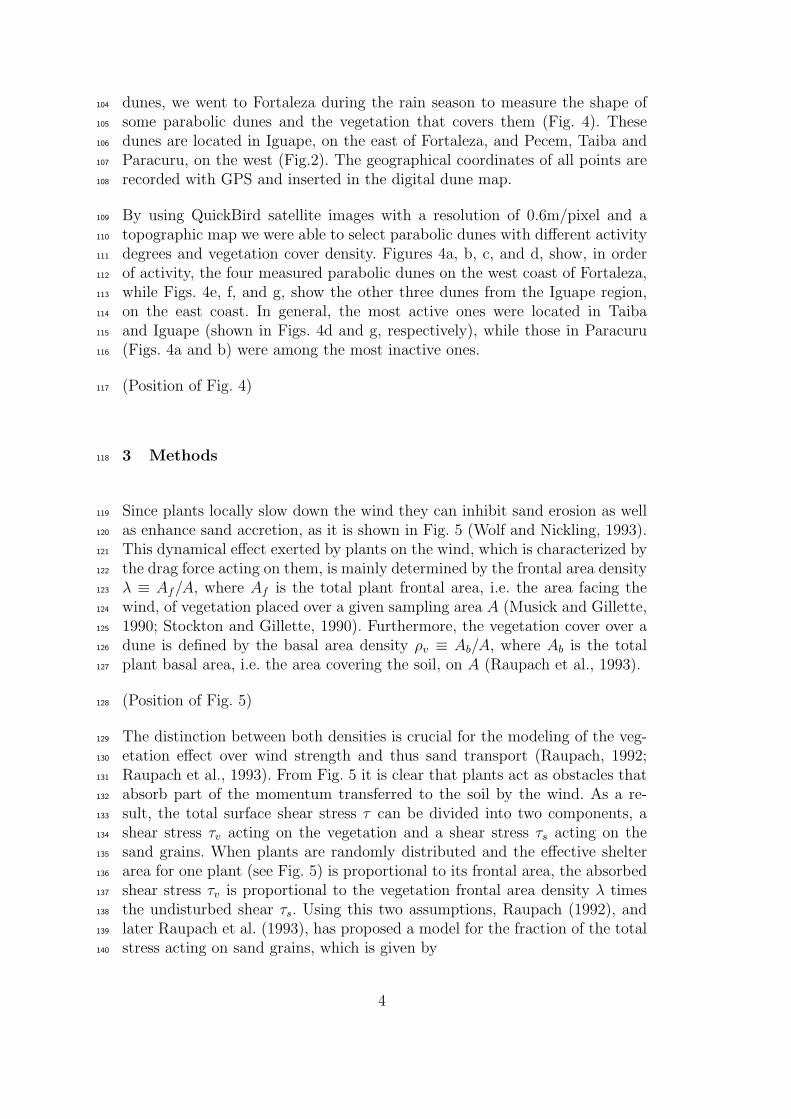
4.1 Wind model204
First, the wind over the surface is calculated with the model of Weng et al.205
(1991) that describes the perturbation of the shear stress due to a smooth hill206
or dune. The Fourier-transformed components of this perturbation are207
7
˜τx =hk2
x
|~k|2
U2(l)
−1 +
2 lnl
z0
+|~k|2
k2x
σK1(2σ)
K0(2σ)
(4)
˜τy =hkxky
|~k|2
U2(l)2√
2σK1(2√
2σ) (5)
where x and y mean, respectively, parallel and perpendicular to the wind208
direction, σ =√
iLkxz0/l, K0 and K1 are modified Bessel functions, and kx209
and ky are the components of the wave vector ~k, i.e. the coordinates in Fourier210
space. h is the Fourier transform of the height profile, U is the vertical velocity211
profile which is suitably non-dimensionalized, l is the depth of the inner layer212
of the flow, and z0 = 1.0mm is the aerodynamic roughness. L is a typical213
length scale of the hill or dune and is given by 1/4 the mean wavelength of214
the Fourier representation of the height profile.215
4.2 Shear stress partitioning216
The effect of the vegetation over the surface wind -shear stress partitioning-217
is calculated by Eq. (1), which gives the fraction τs of total stress τ acting on218
the grains.219
4.3 Sand transport model220
From the modified wind, the sand flux is calculated using the shear velocity221
u∗ =√
τs/ρfluid, where ρfluid = 1.225kg/m3 is the air density, with the equation222
∇ · ~q =|~q|ls
(1− |~q|
qs
), (6)
where223
qs = (2vsα/g)u2∗t[(u∗/u∗t)
2 − 1] (7)
is the saturated flux and224
ls = (2v2sα/γg)/[(u∗/u∗t)
2 − 1] (8)
is called saturation length; u∗t = 0.22m/s is the minimal threshold shear225
velocity for saltation and g = 9.81m/s2 is gravity, while α = 0.43 and γ = 0.2226
are empirically determined model parameters and the mean grain velocity at227
8

saturation, vs, is calculated numerically from the balance between the forces228
on the saltating grains.229
This method for calculating the modified sand transport rate by just taking230
into account the roughness effects on the shear stress, is consistent with the231
field data of Lancaster and Baas (1998) and the wind tunnel data of Al-Awadhi232
and Willetts (1999). However, it neglects more complex interactions between233
saltating grains and plants, in particular when vegetation is higher than the234
maximum saltation height (Gillies et al., 2006).235
4.4 Surface change236
The change in surface height h(x, y) is computed from mass conservation:237
∂h/∂t = −∇ · ~q/ρsand, (9)
where ρsand = 1650kg/m3 is the bulk density of the sand. If sand deposition238
leads to slopes that locally exceed the angle of repose, 34o, the unstable surface239
relaxes through avalanches in the direction of the steepest descent, and the240
separation streamlines are introduced at the dune lee. Each streamline is fitted241
by a third order polynomial connecting the brink with the ground at the242
reattachment point, and defining the “separation bubble”, in which the wind243
and the flux are set to zero.244
4.5 Vegetation growth model245
Finally, the vegetation growth rate is calculated from the surface change using246
the phenomenological equation247
dhv
dt= Vv
(1− hv
Hv
)−∣∣∣∣∣∂h
∂t
∣∣∣∣∣ (10)
where it is assumed that a plant of height hv can grow up to a maximum height248
Hv with an initial rate Vv. To close the model, the basal area density introduced249
in Eq. 1 is just ρv = (hv/Hv)2, and the frontal area density λ = ρv/σ as Fig. 9250
shows. The model is evaluated by performing every step computationally in251
an iterative manner.252
9

5 Results253
5.1 Vegetation cover on real parabolic dunes254
By using the collected vegetation data (reference to TABLE) we are able255
to calculate, through Eqs. (2) and (3), the basal and frontal plant density256
at some particular points on the dunes. The first interesting result is that257
both densities are proportional to each other (Fig. 9) with a proportionality258
constant σ ≈ 1.5 with a reasonable dispersion in spite of the different dunes259
and types of vegetation. Therefore, the plant basal density, also called cover260
density, ρv, can be used to characterize the interaction between vegetation and261
the wind strength given by Eq. (1). This result agrees with measurements on262
Creosote bush reported by Wyatt and Nickling (1997). They also found the263
same value of σ besides the enormous differences in the vegetation type, from264
bush in their case to grass in ours.265
(Position of Fig. 9)266
In order to estimate the degree of activity of the whole parabolic dune, based267
only on the plant cover density, we extend the few measured values of ρv to the268
full dune body using high resolution (0.6 m/pixel) QuickBird panchromatic269
satellite images. Since the figure darkness is mainly determined by the vege-270
tation cover, the simplest approach is to use the brightness index BI, i.e. the271
gray-scale value, of the satellite images. Therefore, a crude phenomenological272
approximation for the cover density at the dune is obtained by relating the273
density cover ρv to its relative brightness index C, defined as274
C ≡ BI −BImin
BImax −BImin
(11)
where BImin and BImax are defined by the normalization conditions ρv(BImin) =275
1 and ρv(BImax) = 0 respectively. These normalization conditions are obtained276
from those points in the image that we know are either bare sand or fully cov-277
ered with plants.278
(Position of Fig. 10)279
Figure 10 shows a clear correlation between both ρv and C for each image.280
By assuming that the cover density decreases linearly with C when C → 1281
and that ρv(C) is symmetric with respect to the main diagonal ρv = C, we282
propose the phenomenological fitting curve283
ρv(C) =1− C
1 + aC(12)
10

where the fitting parameter a changes for different images due to the alteration284
of the respective brightness scale.285
A more sophisticated method for estimating vegetation cover, like NDVI and286
its variants, where C is calculated using the difference between the visible287
red and infra-red bands, should lead to the linear relation ρv = 1 − C, i.e.288
a = 0. However, in our case, since we consider the whole spectrum data to289
estimate C, we also include in our relative brightness value the effect of the290
vegetation shadowing, the biological crust (Levin et al., 2007), the moisture291
content and the organic material mixed with the sand. Remarkably, these292
spurious contributions are apparently contained within the parameter a, which293
then represents just a correction to the linear relation.294
Using equation (12) we can estimate the density cover over the whole parabolic295
dune. Figure 11 shows the resulting density cover calculated from the bright-296
ness index of the images in Fig. 4. Yellow (light) represents free sand, while297
dark green (dark) represents total cover, and thus, total stabilization. With298
the help of the color-scale one identifies the zones where sand transport occurs.299
The windward side in the interior part is the most active part of the dune, as300
consequence of the erosion that prevents plants from growing. On the contrary,301
plants apparently can resist sand deposition since they accumulate clearly at302
the lee side and the crest of the dune.303
(Position of Fig. 11)304
Another important conclusion is that the degree of activation of a dune appar-305
ently depends on its distance from the place where it was born, in concordance306
with previous works (Pye, 1982). The three dunes in Iguape (Fig. 11) are sta-307
bilized according to their distance from the sea shore, the most active being308
the one nearest to the sea (Fig. 11, bottom right). Similarly, the same occurs309
with other studied parabolic dunes.310
Up to here, we have a basic understanding of the morphological characteristics311
of these parabolic dunes, their shape, vegetation cover and relative activation312
degree. However, we lack information about dynamics, which processes are313
behind the formation of these dunes? How they were formed and how they314
will evolved? To partially answer these questions, that contains the key aspects315
of coastal management, we will use the numerical modeling of vegetated dunes.316
5.2 Simulated parabolic dunes317
The model for vegetated sand dunes presented in a previous section, contains318
two set of parameters, one regarding the sand transport and the other con-319
cerning the vegetation growth. Although there are standard values for the320
11

sand transport model, the modeling of vegetation is still an incipient field and321
much more has to be done to properly understand the exact mechanisms and322
parameter behind the interaction of plants and sand transport (Levin et al.,323
2007). In our simple approach, the vegetation growth rate, Eq. (10), is charac-324
terized by two parameters, the initial vegetation growth rate Vv when no sand325
transport occurs, and the maximum height Hv a plant can reach. Besides,326
there are three parameters for the shear stress partitioning Eq. (1), the basal327
to frontal area ratio σ ≡ ρv/λ, the ratio of plant to surface drag coefficients β328
and the constant m. From our measurements only the morphological parame-329
ters can be determined, σ ≈ 1.5 and Hv ≈ 5cm. For the dynamical parameters330
β and m we use reported values for Creosote bush from Wyatt and Nickling331
(1997), β = 200 and m = 0.16.332
The last parameter, the vegetation growth rate Vv, is difficult to determine.333
Notice that in our model Vv is not the biomass production rate, although334
could be related to it, but Vv represents the average vertical growth of the335
plants within a grid point (of about 1m2). However, the grass doesn’t grow to336
much vertically but it mainly expand horizontally beneath the surface, which337
leads to an effective horizontal growth (Danin, 1991). Therefore, for grass338
Vv becomes a horizontal growth (propagation) rate. Following the analysis of339
dune stabilization in Duran and Herrmann (2006) and taking into account340
the high precipitation rates in the zone, we arbitrary select a high growth rate341
Vv = 5m/yr, a value that leads to a low fixation index θ = 0.16 and ensures the342
stabilization process (Duran and Herrmann, 2006). Finally, we use an upwind343
shear velocity of 0.4m/s, consistent with the wind data in the region of Pecem.344
Using these parameters we numerically integrate the model equations starting345
from two different initial conditions: first, an isolated barchan dune devoid346
of vegetation, and second, a blow-out, i.e. a circular spot of bare sand in a347
vegetated surface. As a result, for the first case, once vegetation is allowed to348
growth on the barchan dune, sand transport strongly reduces and the barchan349
evolves toward a parabolic dune (Fig. 12a) (Duran and Herrmann, 2006). In350
the second case, the sand transport inside the blow-out slowly destroys the351
vegetation at its border and a parabolic dune develops (Fig. 12b), which is a352
common case in coastal systems (Pye, 1982; Hesp, 1996).353
(Position of Fig. 12)354
6 Discussion355
From Fig. 12, it is clear that for both initial conditions and the correct com-356
bination of wind shear velocity and vegetation growth rate (Duran and Her-357
rmann, 2006), a parabolic dune evolves with the characteristic vegetated arms358
12

pointing upwind and a sandy windward side. Moreover, the convex and heav-359
ily eroded windward side finishes in a sharp edge vegetated crest, in sharp360
contrast with the barchan dune where the windward side is concave and the361
crest smoothly rounded.362
As can be seen in Fig. 12, it is in the morphology, and not the vegetation363
distribution, where the two parabolic dunes evolving from different initial364
conditions differ most. Although the dunes are of similar sizes, the windward365
side of the blow-out parabolic dune is more than twice the size of the windward366
side of the barchan-born parabolic dune. Furthermore, the blow-out dune is367
more elongated than the corresponding barchan-born one and concentrates a368
higher sand volume in its ‘nose’. This can be understood from their respective369
evolutions: on one hand, the former dune is growing from a spot of bare sand370
in the vegetated surface and its volume is increasing due to the sediment that371
is continuously added on the vegetated surface (Hesp, 1996; Pye, 1982). On372
the other hand, the barchan-born parabolic dune has a total sand volume373
fixed from the beginning and since this volume is distributed over a growing374
surface, the parabolic dune is continuously shrinking, particularly its ‘nose’375
(Duran and Herrmann, 2006).376
After comparing the simulated parabolic dunes (Fig. 12) with the real ones377
from Brazil (Fig. 11) the similarity between the dune emerging from a blow-378
out and the measured ones seems evident. Figure 13 depicts a parabolic dune379
from the Iguape region and its simulated counterpart evolving from a blow-380
out. In this case the gray-scale corresponds to the quantitative vegetation381
cover density ρv (Fig. 13b and d). Although the real dune has twice the size of382
the simulated one, their morphology is very similar. Similarities include: their383
relative length and width; the position of the slip-face, that is sharper along384
the windward side than in the ‘nose’, and the gentile slope in the windward385
side and the front of the ‘nose’ compared to the step lee side.386
Regarding the distribution and density of the vegetation, both dunes also387
share strong similarities (Fig. 13b and d). The distribution of the vegetation388
is clearly divided into two regions, the windward side almost devoid of plants389
and the vegetated lee side (Fig. 14). As was discussed in the previous sections,390
this is a direct consequence of the competition between sand transport and391
vegetation growth, while on the heavily eroded windward side plant roots are392
uncovered and dried, on the lee side they survive sand accretion (see Fig. 14).393
(Position of Figs. 13 and 14)394
However, although the distribution of vegetation is qualitatively similar on395
both dunes, there is an important quantitative difference regarding the veg-396
etation cover density: on the lee side of the simulated dune (Fig. 13d) the397
vegetation density reaches a far higher value, in fact very close to one, than398
13

in the real dune (Fig. 13b). This could be consequence of the way is mod-399
eled the effect of the vegetation on the sand transport. We assume that the400
shear stress partition, i.e. the reduction of the surface wind shear stress, is401
the only way plants can affect the sand transport, but there are other effects.402
For instance, plants act as physical barriers for the saltating grains that are403
carried by the wind (Gillies et al., 2006; Levin et al., 2007). Plants can trap404
them by direct collisions as well as by reducing the wind stress. In this case,405
a given vegetation density can be more effective in avoiding soil erosion than406
when one only considers the wind slow down. This can explain why the lee407
side on both dunes can have the same protecting role while having different408
vegetation density cover.409
7 Conclusions410
We presented measurements on real parabolic dunes along the coast of Brazil,411
concerning their shape and vegetation cover on them. The vegetation cover412
over a dune was estimated by the number and size of plants in a characteristic413
area of the dune. To do so we identify the species of plants present on the dune414
and count the number of times they appear in the study area and measure415
their characteristic length, height and total leaf area.416
By using the vegetation data we were able to calculate the plant cover density417
at particular points on the dunes and compare it with the brightness of the418
satellite image. Doing so we found a relation between both the vegetation419
cover density and the image relative brightness index C which leads us to420
estimate the density cover on the whole parabolic dune. Although this purely421
phenomenological method gives a consistent result for the density cover, it422
clearly introduces a considerable amount of spurious contribution that have423
to be filtered out using direct measurements to calibrate the proposed fitting424
curve (Eq. 12).425
Finally, we compare the empirical vegetation cover data with the result of our426
simulations to validate quantitatively the distribution of vegetation over the427
dune. We conclude that, for the set of parameter studied, the model indeed428
captures the essential aspects of the interaction between the different geomor-429
phological agents, i.e. the wind, the surface and the vegetation. Therefore, by430
using the model predicting power we can estimate the degree of activity of the431
dune and reconstruct the previous dune history. Indeed, the simulations give432
arguments in favor of the possible origin of parabolic dunes on the Brazilian433
coast as developing from blow-outs, rather than from an early active coastal434
crescent dune system, which may represent the response of an unstable coast435
to fluctuations in the wind strength or the precipitation rate. The success-436
fully simulation of a coastal system, an ambitious goal from which this is just437
14

the first step, has far reaching implications in coastal management, it allows438
the study of complex coastal evolution and its stability to changing external439
conditions.440
Acknowledgments441
We wish to thank LABOMAR in Fortaleza for the kind help during the field442
work. This study was supported by the Volkswagenstiftung, the Max Plank443
Prize and the DFG.444
References445
Al-Awadhi, J.M., Willetts, B.B., 1999. Sand transport and deposition within446
arrays of non-erodible cylindrical elements. Earth Surf. Processes Land-447
forms, 24:423-435.448
Anthonsen, K.L., Clemmensen, L.B., Jensen, J.H., 1996. Evolution of a dune449
from crescentic to parabolic from in response to a short-term climatic450
changes, Rabjerg-Mile, Skagen-Odde, Denmark. Geomorphology, 17:63-77.451
Arens, S.M., Slings, Q., de Vries, C.N., 2004. Mobility of a remobilised452
parabolic dune in Kennemerland, The Netherlands. Geomorphology, 50:175-453
188.454
Baas, A.C.W., 2002. Chaos, fractals and self-organization in coastal geomor-455
phology: simulating dune landscapes in vegetated environments. Geomor-456
phology, 48:309-328.457
Baas, A.C.W., Nield, J.M., 2007. Modelling vegetated dune landscapes. Geo-458
phys. Res. Lett., 34:L06405.459
Danin, A., 1991. Plant adaptation in desert dunes. J. Arid Env., 21:193-212.460
Duran, O., Schwammle, V., Herrmann, H.J., 2005. Breeding and solitary wave461
behavior of dunes. Phys. Rev. E, 72:021308.462
Duran, O., Herrmann, H.J., 2006. Vegetation against dune mobility. Phys.463
Rev. Lett., 97:188001.464
Gillies, J.A., Nickling, W.G., King, J., 2006. Aeolian sediment transport465
through large patches of roughness in the atmospheric inertial layer. J. Geo-466
phys. Res., 111:F02006.467
Gillies, J.A., Nickling, W.G., King, J., 2007. Shear stress partitioning in large468
patches of roughness in the atmospheric inertial sublayer. Boundary-Layer469
Met., 122:367-396.470
Hack, J.T., 1941. Dunes of the western Navajo country. Geographical Review,471
31:240-263.472
Hesp, P.A., 1996. Flow dynamics in a trough blowout. Boundary-Layer Mete-473
orology, 77:305-330.474
15
King, J., Nickling, W.G., Gillies, J.A., 2005. Representation of vegetation and475
other nonerodible elements in aeolian shear stress partitioning models for476
predicting transport threshold. J. Geophys. Res., 110:F04015477
King, J., Nickling, W.G., Gillies, J.A., 2006. Aeolian shear stress ratio478
measurements within mesquite-dominated landscapes of the Chihuahuan479
Desert, New Mexico, USA. Geomorphology, 82:229-244.480
Kroy, K., Sauermann, G., Herrmann, H.J., 2002. Minimal model for sand481
dunes. Phys. Rev. Lett., 68:54301.482
Lancaster, N., Baas, A., 1998. Influence of vegetation cover on sand transport483
by wind: Field studies at Owens lake, California. Earth Surf. Proc. and484
Landforms, 23:69-82.485
Levin, N., Kidron, G.J., Ben-Dor, E., 2007a. A field quantification of coastal486
dune perennial plants as indicators of surface stability, erosion or deposition.487
Sedimentology, doi:10.1111/j.1365-3091.2007.00920.x.488
Levin, N., Kidron, G.J., Ben-Dor, E., 2007b. Surface properties of stabilizing489
coastal dunes: combining spectral and field analysis. Sedimentology, 54:771-490
788.491
Muckersie, C., Shepherd, M.J., 1995. Dune phases as time-transgressive phe-492
nomena, Manawatu, New Zealand. Quaternary International, 26:61-67.493
Musick, H.B., Gillette, D.A., 1990. Field evaluation of relationship between a494
vegetation structural parameter and sheltering against wind erosion. Land495
Degradation and Rehabilitation, 2:87-94.496
Nishimori, H., Tanaka, H., 2001. A simple model for the formation of vegetated497
dunes. Earth Surf. Proc. and Landforms, 26:1143-1150.498
Pye, K., 1982. Morphological development of coastal dunes in a humid tropi-499
cal environment, Cape Bedford and Cape Flattery, North Queensland. Ge-500
ografiska Annaler, 64A:213-227.501
Pye, K., Tsoar, H., 1990. Aeolian sand and sand dunes. Unwin Hyman, Lon-502
don.503
Raupach, M.R., 1992. Drag and drag partition on rough surfaces. Boundary-504
Layer Meteorology, 60:375-395.505
Raupach, M.R., Gillette, D.A., and Leys, J.F., 1993. The effect of rough-506
ness elements on wind erosion threshold. Journal of Geophysical Research,507
98:3023-3029.508
Sauermann, G., Kroy, K., Herrmann, H.J., 2001. A continuum saltation model509
for sand dunes. Phys. Rev. E, 64:31305.510
Schwammle, V., Herrmann, H.J., 2005. A model of barchan dunes including511
lateral shear stress. Eur. Phys. J. E, 16:57-65.512
Stockton, P.H., Gillette, D.A., 1990. Field measurements of the sheltering513
effect of vegetation on erodible land surfaces. Land Degradation and Reha-514
bilitation, 2:77-86.515
Tsoar,H., 1990. The ecological background, deterioration and reclamation of516
desert dune sand. Agriculture, Ecosystems and Environment, 33:147-170.517
Tsoar, H., Blumberg, D.G., 2002. Formation of parabolic dunes from barchan518
and transverse dunes along Israel’s Mediterranean coast. Earth Surf. Proc.519
16

and Landforms, 27:1147-1161.520
Tsoar, H., 2005. Sand dunes mobility and stability in relation to climate.521
Physica A, 357:50-56.522
Weng, W.S., Hunt, J.C.R., Carruthers, D.J., Warren, A., Wiggs, G.F.S., Liv-523
ingstone, I., Castro, I., 1991. Air flow and sand transport over sand dunes.524
Acta Mechanica (Suppl.), 2:1-22.525
Wolf, S.A., Nickling, W.G., 1993. The protective role of sparse vegetation in526
wind erosion. Progress in Physical Geography, 17:50-68.527
Wyatt, V.E., Nickling, W.G., 1997. Drag and shear stress partitioning in528
sparce desert Creosote communities. Canadian Journal of Earth Sciences,529
34:1486-1498.530
17

Figure 1 (Color online) Left: Satellite image of active parabolic dunes (de-531
lineated in red) in Pecem along the Brazilian coast. These dunes are partly532
covered by grass (dark tone). Right: Noses of marginally active parabolic533
dunes in Iquape along the Brazilian coast. These dunes are hundreds years534
old and can reach heights up to 50 m. The vegetation that covers them con-535
sist mainly of trees and shrubs. Arrows represent dominant wind direction.536
Figure 2 Map of the north-eastern Brazil province of Ceara illustrating the537
studied region. We measured parabolic dunes along the coast near the city of538
Fortaleza, between the town of Iguape and Paracuru.539
Figure 3 (a) Mean, maximum and minimum monthly precipitation levels540
in the Fortaleza region. As most equatorial-sub-tropical climates, the year is541
clearly divided into a rain season, which here runs from February to July,542
and a dry season. (b) Wind direction and velocity averaged over one month.543
The coastal wind is highly uni-directional, blowing from ESE most of the544
year. Notice that the oscillation of precipitation and wind velocity values have545
opposite phase.546
Figure 4 (Color online) Top: Measured parabolic dunes from Paracuru (a)547
and (b), Pecem (c) and Taiba (d) in decreasing order of activity, the most548
inactive being (a) and the most active (d). Bottom: the other three parabolic549
dunes from Iguape in order of activity, from the less active (e) to the most550
active (g). The bottom right shows a panoramic view of the cluster formed551
by these three dunes. The red (dark) dots on the dunes indicate the loca-552
tion where vegetation was measured (see Fig. 8). North is to top of page553
and wind blows from ESE as shown by the arrow in (a). The geographi-554
cal coordinates of the dunes are: (a) 499912, 9623553, (b) 500754, 9623000, (c)555
513790, 9609650, (d) 510984, 9611800, (e) 572930, 9567090, (f) 573650, 9567200556
and (g) 573990, 9567000.557
Figure 5 (Color online) Strong sand accumulation downwind of a plant due558
to the local wind decrease. Wind blows from left to right. The wind velocity559
in the plant wake is below the threshold for sand transport, which can be560
deduced from the absence of ripples in that region. The effective shelter area561
is enclosed by the circle.562
Figure 6 (Color online) Sketch of the local plant basal area ab covering the563
soil and the frontal area af facing the wind.564
18

Figure 7 (Color online) Left: example of a sampling area used to measure565
the vegetation cover. Right: four typical species of plants found in the region566
where measurements were performed: cyperus maritimus (a), chamaecrista567
hispidula (b), heliotropium polyphyllum (c) and sporobolus virginicus (d).568
Figure 8 (Color online) Satellite image of a typical measured parabolic dune569
with a close up of the vegetation growing in different places over the dune. Red570
(dark) dots indicate the places where vegetation data was collected. North is571
to top of page and wind blows from ESE.572
Figure 9 Proportionality between the basal density ρv ≡ Ab/A and the573
frontal area density λ ≡ Af/A. The proportionality constant of the fit (solid574
line) is Ab/Af ≡ σ = 1.48. Each point represents a different sampling area575
on the dunes situated in Iguape, shown in Fig. 4 bottom, (◦) and the other576
dunes, Fig. 4 top, (•).577
Figure 10 Relation between the vegetation cover density ρv and the relative578
brightness index C from the satellite image. Each point represents another579
sampling area and the plots correspond to: (a) the three dunes from Iguape580
(Fig. 4,e,f and g), (b) the two dunes from Paracuru, (•) (Fig. 4a) and (◦)581
(Fig. 4b), (c) the dune from Pecem (Fig. 4d) and (d) the dune from Taiba582
(Fig. 4c). The fit parameter a in Eq. 12 has the values 0.8, 0.22, 0.08 and 0.18,583
respectively.584
Figure 11 (Color online) Vegetation cover density on the seven measured585
parabolic dunes of the coastal zone of Brazil, depicted in Fig. 4. Yellow (light)586
represents no cover ρv = 0 (C = 1) and dark green (dark) total cover ρv = 1587
(C = 0). The logarithmic color scale is in percentage.588
Figure 12 (Color online) Simulation results: (a) Snapshots of the transfor-589
mation of a barchan dune into a parabolic one. (b) Evolution of a parabolic590
dune from a blow-out. The color-scale, in percentage, represents density cover,591
and, as in Fig. 11, yellow (light) represents no cover ρv = 0 (C = 1) and dark592
total cover ρv = 1 (C = 0). Wind blows from the left.593
Figure 13 (Color online) Comparison between a real and a simulated parabolic594
dune. The morphology of the numerical dune emerging from a blow-out (c) is595
quite similar to the real one found in Iguape (a) (Fig. 4e). The vegetation cover596
19

over the numerical (d) and the real dune (b) also shows the same qualitative597
distribution.598
Figure 14 (Color online) The picture of one arm of a parabolic dune taken599
from the top of its ‘nose’ in the upwind direction, illustrates the difference600
between the internal-windward face, at the left, and the external flanks, at601
the right. In the former the erosion has killed the vegetation, which remnants602
can be seen in dark, while in the lee side the plants are alive. Wind blows out603
of the figure from the left side.604
20

Figure 1
Figure 2
21

Figure 3
Figure 4
22

Figure 5
Figure 6
Figure 7
23

Figure 8
0
0.1
0.2
0.3
0.4
0 0.05 0.1 0.15 0.2 0.25
Ab / A
Af / A
Figure 9
24

0
0.2
0.4
0.6
0.8
1
0 0.2 0.4 0.6 0.8 1
ρ v
C
(a)
0
0.2
0.4
0.6
0.8
1
0 0.2 0.4 0.6 0.8 1
ρ v
C
(b)
0
0.2
0.4
0.6
0.8
1
0 0.2 0.4 0.6 0.8 1
ρ v
C
(c)
0
0.2
0.4
0.6
0.8
1
0 0.2 0.4 0.6 0.8 1
ρ v
C
(d)
Figure 10
Figure 11
Figure 12
25

Figure 13
Figure 14
26