Embed Size (px)
Citation preview

Field measurements and
simulations of supermarkets
with CO2 refrigeration systems
D A V I D F R E L E C H O X
Master of Science Thesis
Stockholm, Sweden 2009

Field measurements and simulations of supermarkets
with CO2 refrigeration systems
David Freléchox
Master of Science Thesis Energy Technology 2009:490
KTH School of Industrial Engineering and Management Division of Applied Thermodynamics and Refrigeration
SE-100 44 STOCKHOLM

Master of Science Thesis EGI 2009/ETT:490
Field measurements and
simulations of supermarkets
with CO 2 refrigeration systems
David Freléchox
Approved
Date Examiner
Björn Palm Supervisor
Samer Sawalha Commissioner
Contact person
Master Student: David Freléchox David Freléchox
Polhemsgatan 34 La Pran 9
11230 Stockholm CH - 2824 Vicques
Registration Number: 821109-A692 (KTH Stockholm)
Registration Number: 650540 (HfT Stuttgart)
Departement: Energy Technology (KTH Stockholm)
Degree Programme: SENCE (HfT Stuttgart)
Examiner at EGI: Prof. Dr. Björn Palm
Supervisor at EGI: Dr. Samer Sawalha
Examiner at HfT: Prof. Dr. Ursula Eicker


KTH Stockholm, Sweden Department of Energy Technology
David Freléchox
I
Abstract
This Master Thesis is a part of a project initiated by Sveriges Energi- & Kylcentrum in
Katrineholm and co-financed by the Swedish energy agency. The project aims to evaluate the
potential of refrigeration systems using carbon dioxide in supermarket refrigeration.
This thesis includes the analysis of three supermarkets using different cooling systems such as
CO2 transcritical chiller unit, CO2 transcritical freezer unit, CO2 transcritical booster unit and
R404A/CO2 cascade unit. The supermarkets have complete instrumentations necessary to
measure temperatures and pressures and measure or evaluate the energy consumptions. The
collected data cover a period of 7 to 18 months. The COP of each system has been evaluated.
Opportunities for improving the regulation of the condensation valve have also been proposed.
CO2 fluid offer possibilities to used floating condensation until a low outdoor temperature and
due to the big pressure difference across the expansion valve, it should still offer improvements
possibilities.
In parallel simulation models of each supermarket were developed using the softwares EES.
The good quality of the collected data allowed validating these models which were then used for
the comparison of the different systems. The COP of each cooling system was being evaluated
in a dynamic manner depending on the condensation temperature, outside temperature and
evaporation temperature. The potential of subcooling and free desuperheating was also
demonstrated.
Several simulations have shown less annual energy consumption for CO2 transcritical plant in
cold and mild climates, as of Stockholm and Frankfurt respectively. On the other hand the
advantage of a cascade system using R404A and CO2 under the hot climate of Phoenix is
evident.
The experimental and theoretical studies reported in this thesis prove that CO2 based system
solutions investigated can be efficient solutions for supermarket refrigeration; however,
comparison with traditional systems is needed and will be presented in following publications in
the ongoing project.
KTH Stockholm, Sweden Department of Energy Technology
David Freléchox
II
Acknowledgements
The ‘CO2 in Supermarket Refrigeration’ project was initiated as an agreement between
Sveriges Energi- & Kylcentrum (SEK) and KTH/Applied Thermodynamics and Refrigeration
Division. The project is managed by SEK and supported by the companies AGA, Ahlsell,
Cupori, Green and Cool, Huurre, ICA, Oppund Svets, Cupori and WICA. This project is also
financed by Energimyndigheten (STEM) and the partner companies. This thesis work is
involved in this project.
First of all, I would like to express my sincere gratitude to my supervisor Samer Sawalha since
this thesis was only possible due to your support and advice. Thanks for your receptiveness and
your unpretentiousness. It was really pleasant working with you.
Secondly, I would like to extend my gratitude to Jörgen Rogstam who is the project manager in
SEK. Thanks for your support, comments and your interest in my work. The project meetings
were always a great source of inspiration for new ways around CO2 refrigeration systems.
Furthermore, I would like to thank my professor from the Master Program “Sustainable Energy
Competence” in the University of Applied Sciences in Stuttgart (HfT), Professor Ursula Eicker,
and also Professor Björn Palm from Applied Thermodynamics and Refrigeration Division of
Energy Technology Department in Royal Institute of Technology (KTH), for giving me the
opportunity to achieve my Master Degree with this great experience in the North.
And I also would like to thank Jigme Nidup for being my support, company and friend during the
months we spent in the laboratory together. That is also for you, Claire and Jean-Remi, for all
the chats we had in the department and for the marvellous moments we shared during this
period here in Sweden.
This thesis is especially dedicated to my parents, Maggy and Mario who supported me all the
time and in all the decision I made during my studies. Thanks for the trust you have in me. It
helps me to enjoy life and grow in this world.
Finally I want to thank you, you who supported my choices, who followed me around Europe,
who helped me during the hard time and who makes life so nice. You are a beautiful person in
your head and in your heart. With all my love, thanks Nancy !
KTH Stockholm, Sweden Department of Energy Technology
David Freléchox
III
Table of contents
ABSTRACT .............................................................................................................................................................................................................I ACKNOWLEDGEMENTS................................................................................................................................................................................... II TABLE OF CONTENTS .....................................................................................................................................................................................III LIST OF FIGURES............................................................................................................................................................................................... V LIST OF TABLES..............................................................................................................................................................................................VII NOMENCLATURE...........................................................................................................................................................................................VIII DEFINITIONS......................................................................................................................................................................................................XI 1 INTRODUCTION......................................................................................................................................................................................... 1
1.1 BACKGROUND................................................................................................................................................ 1 1.2 ENERGY USAGE IN SWEDISH SUPERMARKETS................................................................................................ 2 1.3 REFRIGERANT EMISSIONS............................................................................................................................... 3
2 OBJECTIVES............................................................................................................................................................................................... 4
2.1 BACKGROUND................................................................................................................................................ 4 2.2 PROJECT.........................................................................................................................................................5 2.3 SUMMARY ...................................................................................................................................................... 5 2.4 PROJECT PARTNER......................................................................................................................................... 6
3 CO2 TECHNOLOGY................................................................................................................................................................................... 7
3.1 BACKGROUND................................................................................................................................................ 7 3.2 CO2 AS A REFRIGERANT................................................................................................................................ 8
3.2.1 Properties.............................................................................................................................................. 8 3.2.2 Heat exchange characteristics and high pressure compression.......................................................... 12 3.2.3 Efficiency of CO2 versus synthetic refrigerants .................................................................................. 14
3.3 CO2 SOLUTIONS IN SUPERMARKET REFRIGERATION.................................................................................... 17 3.3.1 Indirect systems................................................................................................................................... 17 3.3.2 Cascade DX systems............................................................................................................................ 18 3.3.3 Transcritical DX systems .................................................................................................................... 19
3.4 SAFETY ISSUES............................................................................................................................................. 20 3.4.1 Concentration levels and safety limits................................................................................................. 20 3.4.2 Case study ........................................................................................................................................... 21
4 MEASUREMENTS AND EVALUATION METHODS ................ .......................................................................................................... 22
4.1 PRESSURE AND TEMPERATURE MEASUREMENTS.......................................................................................... 22 4.2 ELECTRICAL POWER CONSUMPTION; MEASUREMENT OR CALCULATION...................................................... 23 4.3 MASS FLOW EVALUATION............................................................................................................................ 26 4.4 COP CALCULATION ..................................................................................................................................... 31
5 FIELD INSTALLATIONS......................................................................................................................................................................... 33
5.1 SUPERMARKET WITH TRANSCRITICAL SYSTEM TR1..................................................................................... 33 5.2 SUPERMARKET WITH TRANSCRITICAL SYSTEM TR2..................................................................................... 36 5.3 SUPERMARKET WITH CASCADE SYSTEM CC1............................................................................................... 39
6 GENERAL SYSTEM ANALYSIS............................................................................................................................................................. 42
6.1 SUPERMARKET TR1..................................................................................................................................... 42 6.2 SUPERMARKET TR2..................................................................................................................................... 45 6.3 SUPERMARKET CC1..................................................................................................................................... 48 6.4 COMPARISON OF THE THREE SYSTEMS......................................................................................................... 50 6.5 COMPARISON OF THE THREE SYSTEMS WITH A LOAD RATIO OF 3 ................................................................. 53
KTH Stockholm, Sweden Department of Energy Technology
David Freléchox
IV
7 SPECIFIC SYSTEM ANALYSIS.............................................................................................................................................................. 57
7.1 EFFECTS OF THE INSTALLATION OF A FREQUENCY CONVERTER ON THE COMPRESSOR................................. 57 7.2 DISCHARGE PRESSURE VALVE REGULATION................................................................................................ 62 7.3 INFLUENCE OF THE INTERNAL AND EXTERNAL SUPERHEAT ON THE DX CO2 REFRIGERATION SYSTEMS..... 67 7.4 SUBCOOLING WITH GROUND HEAT SINK....................................................................................................... 68 7.5 ANALYSE OF TR2 SYSTEM UNDER TRANSCRITICAL REGIME......................................................................... 71
8 SIMULATION MODEL ............................................................................................................................................................................ 73
8.1 DATA INPUT AND ASSOMPTIONS.................................................................................................................. 73 8.2 FUNCTION TO SIMULATE THE DEPENDENCE OF THE COOLING CAPACITY TO THE OUTDOOR TEMPERATURE.. 76 8.3 FUNCTION TO SIMULATE THE FLUID COMPRESSION...................................................................................... 77 8.4 LIMIT OF THE CONDENSING TEMPERATURE.................................................................................................. 78 8.5 DAY AND NIGHT INFLUENCE ON THE COOLING CAPACITY............................................................................ 79 8.6 VALIDATION OF THE MODELS....................................................................................................................... 81
9 SYSTEMS SIMULATION......................................................................................................................................................................... 83
9.1 VARIATION OF THE CONDENSING TEMPERATURE......................................................................................... 83 9.2 SIMULATION USING IMPROVEMENT POSSIBILITIES FOR CO2 SYSTEMS......................................................... 85 9.3 ANNUAL SIMULATION – COMPARISON OF THE THREE SYSTEMS IN DIFFERENT CLIMATES IN SWEDEN .......... 86 9.4 ANNUAL SIMULATION – COMPARISON OF THE THREE SYSTEMS IN DIFFERENT CLIMATES IN THE WORLD..... 89
10 SPECIFIC SYSTEM SIMULATION................................................................................................................................................... 93
10.1 IMPACT OF THE EVAPORATION TEMPERATURE ON COP ............................................................................... 93 10.2 OPTIMAL CONDENSATION TEMPERATURE FOR THE SUBCRITICAL / TRANSCRITICAL OPERATION TRANSITION
95 10.3 POTENTIAL OF DESUPERHEATING FOR LOW STAGE....................................................................................... 97 10.4 POTENTIAL OF SUBCOOLING WITH GROUND HEAT SINK IN TR2.................................................................... 99
11 DISCUSSION ....................................................................................................................................................................................... 100 12 CONCLUSIONS AND SUGGESTIONS FOR FUTURE WORKS ................................................................................................. 103 13 REFERENCES..................................................................................................................................................................................... 104 APPENDIX 1: FORMULA COPTOT WITH LOAD RATIO CORRECTI ON ............................................................................................ 106
KTH Stockholm, Sweden Department of Energy Technology
David Freléchox
V
List of Figures
Figure 1.1: A breakdown of energy usage in a supermarket in Sweden. (Arias, 2005)........................................................................2 Figure 3.1: h-logP diagram for the CO2 (left) and the R134a (right)....................................................................................................8 Figure 3.2: Saturation pressure versus temperature for selected refrigerants (Sawalha, 2008)...........................................................9 Figure 3.3: Latent heat of vaporization / condensation (left), saturated vapour density (right) for selected refrigerants (Sawalha,
2008).........................................................................................................................................................................................9 Figure 3.4: Volumetric refrigeration capacity for selected refrigerants (Sawalha, 2008) ....................................................................10 Figure 3.5: Isobaric specific heat of CO2 (left), Isobaric Prandtl number of CO2 (right) (Kim et al., 2003).........................................12 Figure 3.6: Liquid to vapour density (left), surface tension versus saturated temperature for selected refrigerants (Sawalha, 2008).13 Figure 3.7: Compressor pressure diagrams for R134a and CO2 assuming equal cooling capacity (π: pressure ratio, pm: mean
effective pressure) (Kim et al., 2003) .......................................................................................................................................14 Figure 3.8: Comparison of thermodynamic cycles for R134a and CO2 in temperature-entropy diagrams, showing additional
thermodynamic losses for the CO2 cycle when assuming equal evaporating temperature and equal minimum heat rejection temperature(left) (Kim et al., 2003); Comparison of thermodynamic cycles for R134a and CO2 in temperature-entropy diagrams, when assuming equal evaporating temperature and equal logarithmic mean temperature difference(right) (Sawalha, 2009).......................................................................................................................................................................................15
Figure 3.9: Average monthly COP of CO2 and R404A medium (left) and low (right) temperature unit in the climate of Treviso (Italy). (Girotto et al., 2004) ................................................................................................................................................................15
Figure 3.10: Comparison of R404A and CO2 for energy efficiency, medium temperature refrigeration, single stage compressor, direct expansion, no heat recovery. (Haaf, 2005).....................................................................................................................16
Figure 3.11: Secondary fluid systems with phase change. (Girotto, 2005)........................................................................................17 Figure 3.12: Direct expansion system in cascade. (Girotto, 2005) ....................................................................................................18 Figure 3.13: Direct expansion system and transfer of heat directly into the environment. (Girotto, 2005)..........................................19 Figure 3.14: CO2 concentration limit for many safety levels. (Sawalha, 2009)..................................................................................20 Figure 3.15: CO2 concentration against time in a shopping area for leakage durations of 15 minutes, 30 minutes, 1 hour and 2
hours. (Sawalha ,2008) ...........................................................................................................................................................21 Figure 4.1: Schematic of a CO2 Transcritical Supermarket with the pressure and temperature measurement points. ......................23 Figure 4.2: Compressor electrical power measured for one day in July 2008 (01.07.08) in TR1 Supermarket. .................................24 Figure 4.3: Compressor’s electrical power consumption as a function of the pressure ratio for Bitzer compressors in CC1
supermarket. ...........................................................................................................................................................................24 Figure 4.4: Electrical power consumption, comparison with the two methods for a single stage CO2 system during the whole year
2008, KA1 unit in the TR1 Supermarket. .................................................................................................................................25 Figure 4.5: Volumetric efficiency based on compressor data for three CO2 compressors.................................................................26 Figure 4.6: Mass flow of CO2 in the freezer system FA1 during one day of July 2008 in the TR1 supermarket ................................27 Figure 4.7: Mass flow of CO2 in a transcritical system for different mass flow measurement method ...............................................28 Figure 4.8:COP of a CO2 transcritical system for different mass flow measurement method............................................................30 Figure 5.1: Freezer unit in TR1 Supermarket....................................................................................................................................33 Figure 5.2: Schematic diagram of the TR1 system ...........................................................................................................................34 Figure 5.3: Booster unit in TR2 Supermarket....................................................................................................................................36 Figure 5.4: Schematic diagram of the TR2 system ...........................................................................................................................37 Figure 5.5: Two CO2 low temperature units in the CC1 supermarket ...............................................................................................39 Figure 5.6: Schematic diagram of the cooling system in the supermarket CC1.................................................................................40 Figure 6.1: Cooling capacity of one medium temperature unit (KA1) and one low temperature unit (FA1) during the years 2008 -
2009........................................................................................................................................................................................42 Figure 6.2: Compressors electrical power consumption for one medium temperature unit (KA1) and one low temperature unit (FA1)
during the years 2008 - 2009...................................................................................................................................................43 Figure 6.3: COP function of coolant temperature for medium temperature units and low temperature units, measures for TR1
supermarket during 2008.........................................................................................................................................................44 Figure 6.4: COP for each units during the whole testing period for the TR1 supermarket. ................................................................44 Figure 6.5: Different parameters plots for the KAFA1 unit during the whole period of study in the TR2 supermarket ........................45 Figure 6.6: Different parameters plots for the KAFA2 unit during the whole period of study in the TR2 supermarket ........................46 Figure 6.7: Different parameters plots for the KA3 unit during the whole period of study in the TR2 supermarket.............................46 Figure 6.8: COP for each units during the whole testing period for the TR2 supermarket. ................................................................47 Figure 6.9: Cooling capacity, compressor electrical power consumption, condensation and outside temperatures for medium
temperature units VKA1 and VKA2 during the whole testing period for the CC1 supermarket .................................................48 Figure 6.10: Cooling capacity, compressor electrical power consumption, condensation and outside temperatures for low
temperature units KS5 and KS6 during the whole testing period for the CC1 supermarket ......................................................49 Figure 6.11: COP for each units during the whole testing period for the CC1 supermarket. ..............................................................49 Figure 6.12: Load ratio for the three systems analysed during each period of analysis.....................................................................50 Figure 6.13: Condensation temperature for the three systems analysed during each period of analysis...........................................51 Figure 6.14: Condensation temperature for the three systems analysed during each period of analysis...........................................52 Figure 6.15: Load ratio correction for the three systems during the whole period of analysis ............................................................53 Figure 6.16: Total COP with a load ratio of 3 in function of the condensing temperature for the three systems analysed..................54 Figure 6.17 Total COP with a load ratio of 3 in function of the condensing temperature for the three systems analysed, TR1 system
with elimination of the borehole subcooling effect. ...................................................................................................................54 Figure 6.18: Condensation temperature versus outside temperature fort he three systems..............................................................55 Figure 6.19: Total COP with a load ratio of 3 in function of the outside temperature for the three systems analysed ........................56
KTH Stockholm, Sweden Department of Energy Technology
David Freléchox
VI
Figure 7.1: Electrical power consumption of the compressors in KA2 during March 2009.................................................................57 Figure 7.2: Suction pressure and evaporation temperature of KA2 during March 2009.....................................................................58 Figure 7.3: Internal and external Superheat of KA2 during March 2009............................................................................................59 Figure 7.4: Suction pressure and evaporation temperature of FA2 during March 2009.....................................................................60 Figure 7.5: Daily average of the compressor electrical power and coolant temperature for KA2 during March 2009.........................61 Figure 7.6: Comparison the two KA units of TR1 after the installation of a frequency converter on KA2. ..........................................62 Figure 7.7: CO2 transcritical cycle with gas cooler exit temperature of 40°C at different discharge pr essure (left), (Sawalha, ( 2008) –
Danfoss ICM/ICAD Valve for condensation regulation (right) (Danfoss Refrigeration, 2006)....................................................63 Figure 7.8: IWMAC interface for compressor and gas cooler for KA2, 27 April 2009, 14h10.............................................................63 Figure 7.9: Opening of the discharge pressure regulation valve for KA1 during March 2009 ............................................................64 Figure 7.10: Subcooling of KA1 during March 2009..........................................................................................................................65 Figure 7.11: High pressure for KA1 before the ICAD valve (HP) and after the ICAD valve (HP before exp. Valve) during March 2009.
................................................................................................................................................................................................65 Figure 7.12: EES visualisation on the h-logP diagram for the two condensation regulation functions, KA1 during March 2009.........66 Figure 7.13: Effect of the internal and external superheat on the COP by using CO2 in standard refrigeration system.....................67 Figure 7.14: COP improvement due to the subcooling with the heat sink for KA3 medium temperature unit in TR2 supermarket . ...69 Figure 7.15: Isotherme shape in h-logP diagramm for CO2 near critical point ..................................................................................70 Figure 7.16: Effect on the COP of the subcooling at different condensation temperature for CO2 and R404A with an evaporation
temperature at -10°C and an internal superheat of 1 0 K. .........................................................................................................70 Figure 7.17: KA3 unit in TR2 system during one week at the end of June 2009................................................................................71 Figure 7.18: KA3 unit from TR2 system during two days at the end of June 2009 ............................................................................72 Figure 7.19: KAFA1 unit in TR2 system during four days at the end of June 2009............................................................................72 Figure 8.1: Function binding the percentage used of the maximal cooling capacity to the outdoor temperature................................76 Figure 8.2: Total efficiency of 3 CO2 compressors types in function of the pressure ratio.................................................................77 Figure 8.3: Day and night trend of the cooling capacity of the KA3 unit in the supermarket TR2 during February 2009. ...................80 Figure 8.4: Function binding the percentage used of the maximal cooling capacity to the outdoor temperature with variation range + /
- 25% for a typical medium temperature cabinet. .....................................................................................................................81 Figure 8.5: Comparison of the COP between the template calculation and the EES simulation........................................................82 Figure 9.1: Total COP for different condensation temperature..........................................................................................................83 Figure 9.2: Total COP for different outside temperatures..................................................................................................................84 Figure 9.3: Total COP for different outside temperatures using improvements possibilities for CO2 systems ...................................85 Figure 9.4: Number of hours per year for different outside temperature levels in Storön, Göteborg and Floda – the three locations
are in Sweden. ........................................................................................................................................................................87 Figure 9.5: Annual energy consumption for different supermarket systems in Storön, Göteborg and Floda – all three locations are in
Sweden. ..................................................................................................................................................................................88 Figure 9.6: Number of hours per year for different outside temperature levels in Stockholm / Sweden, Frankfurt / Germany and
Phoenix – Arizona / USA. ........................................................................................................................................................89 Figure 9.7: Annual energy consumption for different supermarket systems in Stockholm / Sweden, Frankfurt / Germany and Phoenix
– Arizona / USA.......................................................................................................................................................................90 Figure 9.8: Annual energy consumption with or without coolant loop for different supermarket systems in Stockholm / Sweden,
Frankfurt / Germany and Phoenix – Arizona / USA..................................................................................................................91 Figure 10.1: COP for medium and low temperature system at different evaporation temperatures on the TR1 system.....................93 Figure 10.2: Relative impact of the evaporation temperature on low and medium temperature systems with reference evaporation
temperatures at -10°C and -35°C. ................... ........................................................................................................................94 Figure 10.3: Enthalpy condenser – gas cooler outlet at different condensation temperature and for two transition temperatures 28
and 30°C. .......................................... ......................................................................................................................................95 Figure 10.4: Total COP and discharge pressure versus the condensing temperature for different transition temperatures with the
supermarket TR2 system (2Transcritical booster units and one chiller unit).............................................................................96 Figure 10.5: Total COP improvement in percentage with a transition temperature at 28°C instead of 31°C related to the Figure 9.2
as usual for a load ratio of 3. ...................................................................................................................................................97 Figure 10.6: Total COP for the supermarket CC1 with and without free desuperheat on the low temperature unit............................98 Figure 10.7: Effect of the ground heat sink when it is using to subcool the liquid in TR2 supermarket ..............................................99
KTH Stockholm, Sweden Department of Energy Technology
David Freléchox
VII
List of tables
Table 7-1: Monthly average of the electrical power consumption for KA2 and FA2...........................................................................61 Table 7-2: List of performance data when one compressor is running for KA1 and FA1 for March 2009 before and after changing the
function of the regulation valve. ...............................................................................................................................................66 Table 8-1: Data input and assumptions for the simulations...............................................................................................................74 Table 9-1: Annual energy consumption excess in percentage in comparison with the better system for each supermarket systems in
Storön, Göteborg and Floda. ...................................................................................................................................................88 Table 9-2: Annual energy consumption excess in percentage in comparison with the better system for each supermarket systems in
Stockholm / Sweden, Frankfurt / Germany and Phoenix – Arizona / USA. ...............................................................................92
KTH Stockholm, Sweden Department of Energy Technology
David Freléchox
VIII
Nomenclature
Roman
A Area [m2]
C Concentration [PPM]
CC Cascade refrigeration system
22 COorCO Carbone dioxide
COP Coefficient of performance [-]
pc Specific heat [kJ/kg*K]]
CR Circulation ratio [-]
d Pipe diameter [m]
dP Pressure drop [kPa]
dT Temperature drop [K]
DX Direct expansion
E& Electrical power [kW]
EES Engineering Equation Solver
f Friction factor [-]
FA Low temperature unit or cabinet
h Enthalpy [kJ/kg]
fgh Latent heat of vaporization [kJ/kg]
IDLH Immediately Dangerous to Life or Heath
IHE Internal heat exchanger
KA Medium temperature unit or cabinet
KAFA Booster system with low and medium temperature
L Pipe length [m]
LTMD Logarithmic Mean Temperature Difference [K]
LR Load ratio
corrLR Load ratio correction, fixed value
m& Mass flow [kg/s]
n Rotational speed [rpm]
33 NHorNH Ammonia
KTH Stockholm, Sweden Department of Energy Technology
David Freléchox
IX
Nu Nusselt Number [-]
P Pressure [bar absolute]
PPM Parts per Million
Pr Prandtl Number [-]
PR Pressure ratio [-]
cQ& Condensation capacity [kW]
oQ& Cooling capacity [kW]
vq Volumetric refrigeration effect [kJ/m3]
Re Reynolds Number [-]
SC Subcritical refrigeration system
SH Superheat [K]
T Temperature [°C]
TR Transcritical refrigeration system
V& Volume flow [m3/s]
w Velocity [m/s]
x Vapour quality [-]
*x Position along the heat exchanger [m]
Y Constant [kW2/m4]
Greek
α Heat transfer coefficient [W/m2*K]
∆ Difference [-]
ε Heat exchanger effectiveness [-]
λ Thermal conductivity [W/m*K]
ρ Density [kg/m3]
isη Isentropic efficiency [-]
vη Volumetric efficiency [-]
totη Total efficiency [-]
µ Dynamic viscosity [kg/s*m]
ν Specific volume [m3/kg]

KTH Stockholm, Sweden Department of Energy Technology
David Freléchox
X
Subscript
abs Absolute
air For air
amb Ambient
app Approach temperature difference
booster Booster system
cab Cabinet medium temperature
chiller Chiller
comp Compressor
cond Condenser
el Electric
evap Evaporation
in Inlet
is Isentropique
f Fluid
freezer Freezer
gc Gas cooler
losses Heat losses
map Map or design conditions
new New or running conditions
out Outlet
cooleroil Oil cooler losses
s Surface
sat Saturation
KTH Stockholm, Sweden Department of Energy Technology
David Freléchox
XI
Definitions
CFC: Chlorofluorocarbon is any of various halocarbon compounds consisting of
carbon, hydrogen, chlorine, and fluorine.
GWP: Global Warming Potential. The GWP is a measure of how much a given mass of
greenhouse gas is estimated to contribute to global warming. It is a relative scale
which compares the gas in question to that of the same mass of carbon dioxide
(whose GWP is by definition 1). A GWP is calculated over a specific time interval
and the value of this must be stated whenever a GWP is quoted or else the value
is meaningless.
HCFC: Hydro chlorofluorocarbons are halogenated compounds containing carbon,
hydrogen, chlorine and fluorine. They have shorter atmospheric lifetimes than
CFCs and deliver less reactive chlorine to the stratosphere where the “ozen
layer” is found.
HFC: Hydro fluorocarbons contain no chlorine. They are composed entirely of carbon,
hydrogen, and fluorine. They have no known effects at all on the ozone layer.
Only compounds containing chlorine and bromine are thought to harm the ozone
layer. Fluorine itself is not ozone-toxic. However, HFCs and perfluorocarbons do
have activity in the entirely different realm of greenhouse gases, which do not
destroy ozone, but do cause global warming. Two groups of haloalkanes, hydro
fluorocarbons (HFCs) and perfluorocarbons (PFCs), are targets of the Kyoto
Protocol.
ODP: Ozone Depletion Potential. The ODP of a chemical compound is the relative
amount of degradation to the ozone layer it can cause, with
trichlorofluoromethane (R-11) being fixed at an ODP of 1.
Source: Wikipedia.org and Wikipedia.fr, 10th march 2009
KTH Stockholm, Sweden Departement of Energy Technology
David Freléchox
1
1 Introduction
1.1 Background
Following the depletion problems of the ozone layer through the release of CFC refrigerant or
HCFCs in the atmosphere, the politicians decided through the Montreal Protocol in 1987 to
prohibit the use of these substances. CFCs are forbidden since 1996 and HCFCs about in
2010. The chemistry has proposed a new type of synthetic fluid called HFCs. These Hydro-
Fluoro-Carbons did not contain the chlorine molecule responsible for the depletion of the ozone
layer any more and showed promise. The ozone layer damaging problem is gently solving but
the problem related to the refrigerant has changed to the increase of the greenhouse effect on
the earth. HFCs have an ODP-Value (Ozone Depletion Potential) of zero given the absence of
chlorine in their structure, but they still have a high GWP value (Global Warming Potential). For
example R404A has a GWP value of 3800 that is much higher than the reference fluid, CO2,
which has a GWP value of 1. This has led to their integration into the Kyoto Protocol, which is in
application since 2005, and implicates various restrictive measures. HFCs emissions control is
imposed and reduction of global emissions are established. This is translated into reality by
limiting the amount of HFC fluids in the refrigeration systems and other periodic leak mandatory.
The ultimate objective is to prohibit the use of these substances.
The search for an adequate and satisfactory solution has resulted in the proposal of a returning
to natural refrigerants. NH3, most commonly ammonia and CO2 or carbon dioxide came back to
use after a widespread application in the early of the 20th century. In commercial refrigeration,
CO2 is favoured despite thermodynamic properties being not quite as good as NH3. It has a
main safety advantage over NH3 which can be dangerous already at relatively low
concentrations.
However, the use of a natural refrigerant will not solve the problems attached to the
environment if it consumes more energy. The solution has to take into account the direct and
indirect impact of the cooling solution on the environment. The new designed system using
natural refrigerant must match or surpass the energy efficiency of old solutions.
KTH Stockholm, Sweden Department of Energy Technology
David Freléchox
2
1.2 Energy usage in Swedish supermarkets
Traditionally, supermarkets have always been major consumers of energy, particularly of
electrical energy for lighting and for the refrigeration systems. According to Orphans (1997), the
share of energy used from the U.S. and French supermarkets reach 4% of the national energy
consumption. Regulations and needs for the conservation of fresh and frozen products do not
offer many saving possibilities to decrease the cooling capacity and energy consumption of the
refrigeration system.
To reduce electrical consumption in supermarkets, research in more efficient systems is
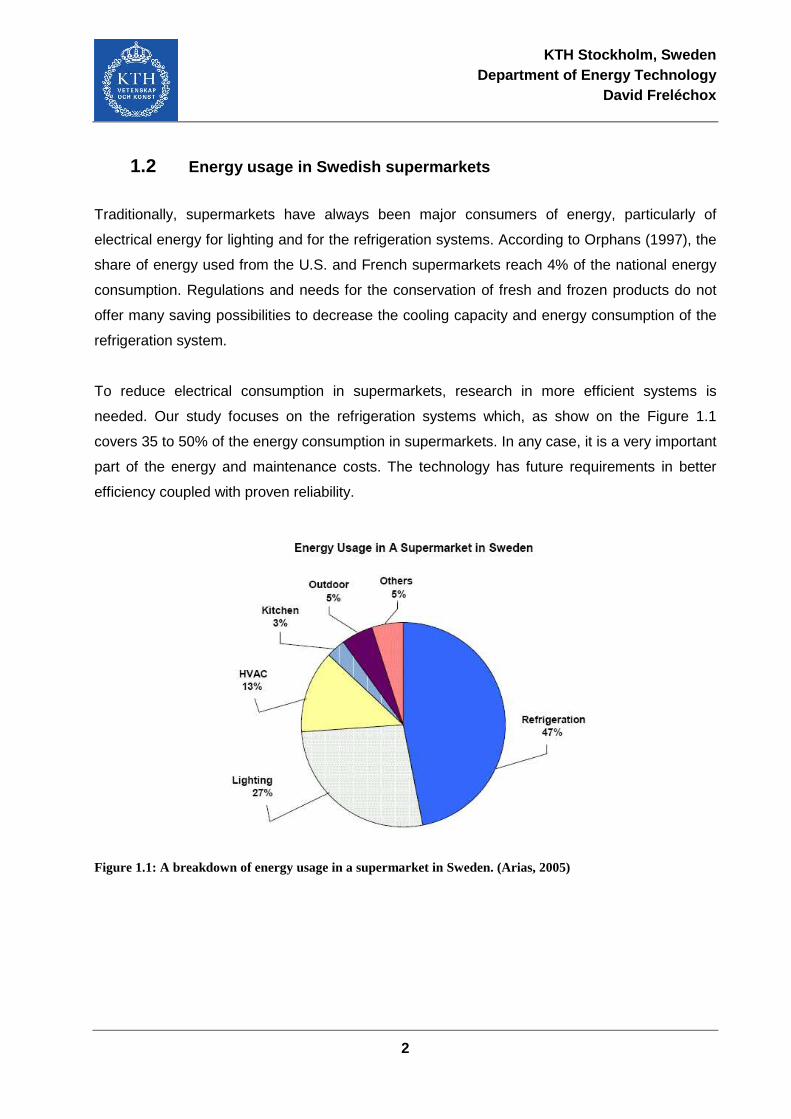
needed. Our study focuses on the refrigeration systems which, as show on the Figure 1.1
covers 35 to 50% of the energy consumption in supermarkets. In any case, it is a very important
part of the energy and maintenance costs. The technology has future requirements in better
efficiency coupled with proven reliability.
Figure 1.1: A breakdown of energy usage in a supermarket in Sweden. (Arias, 2005)
KTH Stockholm, Sweden Department of Energy Technology
David Freléchox
3
1.3 Refrigerant emissions
The impact of refrigerant leakage on the environment has affected the design of refrigeration
systems in supermarkets. Commercial refrigeration is the sector with the largest refrigerant
emissions totalling about 185,000 metric tonnes in 2002, which is equivalent to 37% of the
worldwide refrigerant emissions [PAL04].
Commercial refrigeration systems refrigerant emissions in the 1980’s were reported to be in the
range of 20-35% of refrigerant charge on an annual basis for developed countries. The high
emission rates were due to design, construction, installation, and service procedures followed
without awareness of potential environmental impact. Emissions have been decreasing due to
industry actions and governmental regulations for refrigerant containment, recovery, and usage
record keeping, increased personnel training, improved service procedures, and attention to
many details in system design [BIV04].
These enormous leakage rates have gradually decreased thanks to the use of more reliable
montage technique, reducing fluid amount through the use of indirect systems and the
introduction of a variety of regulations resulting in higher prices of refrigerants. The annual
leakage rate of this century is generally around 10%.
Bivens and Gage in their study from 2004 compare several European countries. Briefly and
generally, Germany announced an annual rate of leakage of 10% for a series of supermarket
with R404A. Denmark is also in this range but including all types of refrigerants. Norway
announced a rate of 14% following a study between 2002 and 2003. Sweden has improved its
annual rate from 14.0% in 1993 to a rate of 10.4% in 2001. In this case, there is a large disparity
between the fluids. Finally, the Netherlands is the best cited example. Since 1992, the country
has implemented strict regulation for the use of refrigerants with the creation of a special
structure (STEK) to reduce emissions of refrigerant. A Dutch report from 1999 is cited which
demonstrated the effectiveness of this process with an annual leakage rate of 3.2%.
KTH Stockholm, Sweden Department of Energy Technology
David Freléchox
4
2 Objectives
The main objective of this project is to analyze and then compare the energy performance of
several supermarkets using CO2 as refrigerant. The supermarkets use different cooling system
configurations, and a simulation tool is essential to achieve comparisons. The in-situ
measurements allow validating these simulations which are then used to analyze the
performance of each system according to different variables or under different climates.
2.1 Background
This project is run by Sveriges Energi & Kylcentrum (SEK) which is a subsidiary company of
Installatörernas Utbildingscentrum in Katrineholm, in cooperation with KTH. Using CO2 as a
refrigerant in supermarkets is becoming increasingly popular in Sweden. It is a promising
technology which offers opportunities in energy savings and protecting the environment. CO2
has been used as refrigerant in different system solutions: transcritical, cascade and indirect.
The efficiency of each system solution depends on several parameters such as the system
capacity, heating requirements, climate conditions, etc. Proper evaluation of the currently
installed CO2 system solutions is needed to facilitate the application of the new technology.
This project is a continuation of the work that has been conducted by KTH in cooperation with
Sveriges Energi & Kylcentrum (SEK). The application of CO2 in supermarket refrigeration has
been theoretically and experimentally investigated. Computer simulation models have been built
for the theoretical analysis of the different CO2 system solutions.
KTH Stockholm, Sweden Department of Energy Technology
David Freléchox
5
2.2 Project
In this project several supermarket installations with different CO2 systems and conventional
solutions will be evaluated. The main tasks in the project are to build the measuring equipment,
install it in the supermarkets and to create the templates for collecting the data and to run the
calculations. The task in the MSc thesis work includes analysis of data from the field
measurements, focus will be on system’s cooling performance and efficiency. Computer models
will be used to simulate the performance of the different system solutions. Compare the field
measurements with the results from the computer simulation models. Performance of the
different system solutions will be compared and suggestions for modifications will be made.
In summary, the following schedule has been followed:
� Documentation on CO2 refrigerating technology
� Collecting data on refrigeration systems
� Creating a database for each supermarket
� Data processing, calculation of needed thermodynamic parameters
� Modifications and adaptations of existing computer simulations for each system
� Calculation of the COP using the measurements and the computer models
� Model validations
� Proposition for improvements to optimize energy efficiency
2.3 Summary
The work in this thesis started by surveying three existing CO2 supermarket installations in
Sweden. Pressures, temperature and energy consumption were collected for different periods in
each supermarket. A template in order to calculate all the thermodynamic states of the systems
was created, cooling capacities and COP of each system were calculated.
The approach of this experimental project allows evaluating the performance of each
refrigeration system and compare them. Through the online data collection for three running
supermarkets, it is possible to assess the influence of external parameters, such as outside
temperature and/or evaporation temperature, and demonstrate their influence on the energy
consumption of various CO2 refrigeration systems.
KTH Stockholm, Sweden Department of Energy Technology
David Freléchox
6
In order to perform theoretical evaluations of the performance of different CO2 system solutions
computer simulation models have been used to simulate CO2 transcritical parallel system, CO2
transcritical booster system and R404A/CO2 cascade system. Based on the measurement a
validation of the model has been achieved.
After studying the modifications made by the installer on different supermarkets and in
combination with the simulations based on the computer models, performance evaluation and
analysis of systems’ optimizations have been done. Suggestions for improvements and
recommendations for future research topics have subsequently been drafted.
This project will facilitate further development of refrigerating system using CO2 as refrigerant; it
will also provide answers on the efficiency of these systems and the possibility of using CO2 as
a long term solution in supermarket refrigeration.
2.4 Project partner
Organization: Participant/s:
Sveriges Energi- & Kylcentrum Institution Jörgen Rogstam
KTH – Energiteknik University Björn Palm / Samer Sawalha
ICA Supermarket Per-Erik Jansson
Green and Cool Supplier Micael Antonsson
WICA Supplier Peter Rylander
Ahlsell Installer Torbjörn Larsson
Huurre Installer Göran Sundin
AGA Christer Hens
Tranter Ulf Vestergren
Cupori David Sharp
Oppunda Svets Ken Johansson
Energimyndigheten Conny Ryytty
KTH Stockholm, Sweden Department of Energy Technology
David Freléchox
7
3 CO2 Technology
3.1 Background
The use of CO2 as refrigerant was widespread at the end of the 19th and the beginning of the
20th Century, particularly in the applications of marine refrigeration. Thereafter, with the
appearance of new synthetic refrigerants like CFC, its use has gradually reduced until its
complete abandonment. [KIM03]
The reasons are relatively easily identifiable; the synthetic refrigerants generally work at a lower
pressure, which make the implementation easier during the assembly facilities. Component
manufacturers have also been able to maintain a competitive price for their components for this
reduced pressure. The relatively low temperature at the critical point for CO2 also caused
difficulties in providing the required capacity. The systems used did not work at optimal
transcritical operation which caused technical difficulties and efficiency losses.
Currently, we are witnessing a renaissance of this fluid for refrigeration applications. Its absence
of effect on the ozone layer and its minimal impact on the greenhouse effect compared to
synthetic refrigerants made it as a favourite alternative from environmental point of veiw. This
renaissance is largely attributed to the work of Professor Gustav Lorentzen who suggested the
use of CO2 in a transcritical cycle during the end of the 1980s [SAW08]. His solution for the
automotive air-conditioning has subsequently led to work on other applications, such as
commercial refrigeration and led about 15 years later on the construction of the first
supermarkets with CO2 transcritical application.
The CO2 has several interesting characteristics; it is non-flammable, non-explosive and
relatively non-toxic. It is present in the air at a concentration of 350-400 PPM. As stated its ODP
value is zero and its GWP value is very low, 1.
KTH Stockholm, Sweden Department of Energy Technology
David Freléchox
8
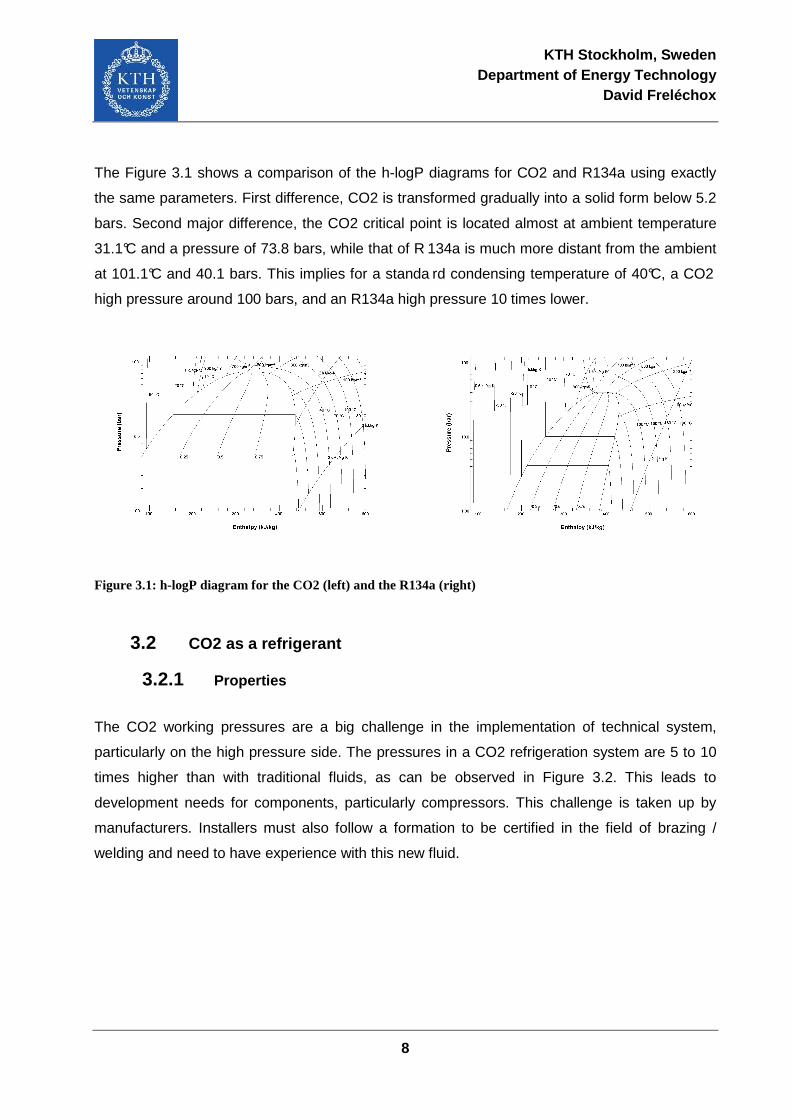
The Figure 3.1 shows a comparison of the h-logP diagrams for CO2 and R134a using exactly
the same parameters. First difference, CO2 is transformed gradually into a solid form below 5.2
bars. Second major difference, the CO2 critical point is located almost at ambient temperature
31.1°C and a pressure of 73.8 bars, while that of R 134a is much more distant from the ambient
at 101.1°C and 40.1 bars. This implies for a standa rd condensing temperature of 40°C, a CO2
high pressure around 100 bars, and an R134a high pressure 10 times lower.
Figure 3.1: h-logP diagram for the CO2 (left) and the R134a (right)
3.2 CO2 as a refrigerant
3.2.1 Properties
The CO2 working pressures are a big challenge in the implementation of technical system,
particularly on the high pressure side. The pressures in a CO2 refrigeration system are 5 to 10
times higher than with traditional fluids, as can be observed in Figure 3.2. This leads to
development needs for components, particularly compressors. This challenge is taken up by
manufacturers. Installers must also follow a formation to be certified in the field of brazing /
welding and need to have experience with this new fluid.
KTH Stockholm, Sweden Department of Energy Technology
David Freléchox
9
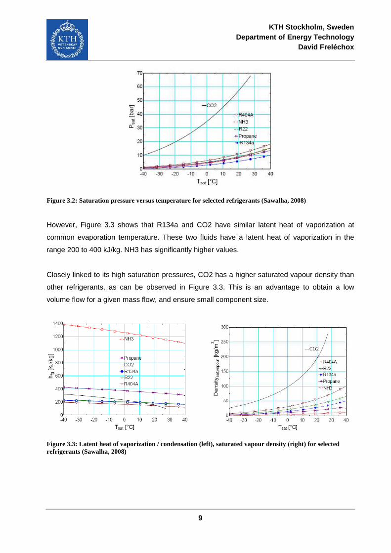
Figure 3.2: Saturation pressure versus temperature for selected refrigerants (Sawalha, 2008)
However, Figure 3.3 shows that R134a and CO2 have similar latent heat of vaporization at
common evaporation temperature. These two fluids have a latent heat of vaporization in the
range 200 to 400 kJ/kg. NH3 has significantly higher values.
Closely linked to its high saturation pressures, CO2 has a higher saturated vapour density than
other refrigerants, as can be observed in Figure 3.3. This is an advantage to obtain a low
volume flow for a given mass flow, and ensure small component size.
Figure 3.3: Latent heat of vaporization / condensation (left), saturated vapour density (right) for selected refrigerants (Sawalha, 2008)
KTH Stockholm, Sweden Department of Energy Technology
David Freléchox
10
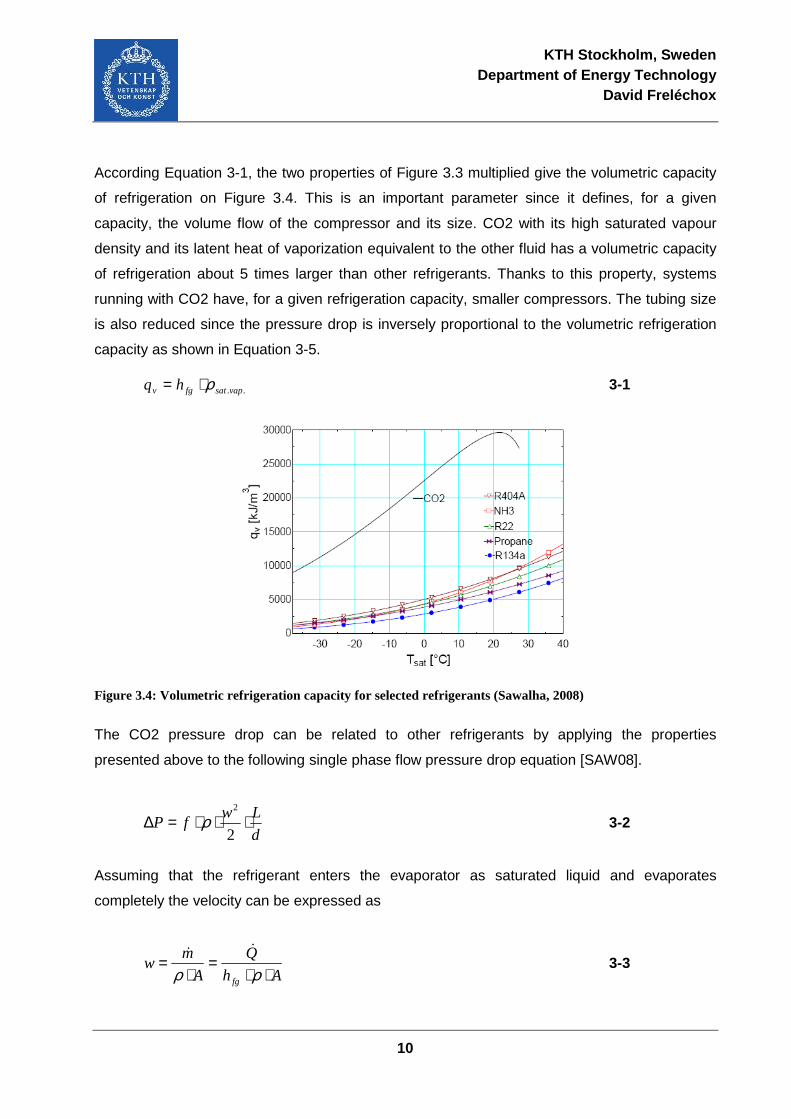
According Equation 3-1, the two properties of Figure 3.3 multiplied give the volumetric capacity
of refrigeration on Figure 3.4. This is an important parameter since it defines, for a given
capacity, the volume flow of the compressor and its size. CO2 with its high saturated vapour
density and its latent heat of vaporization equivalent to the other fluid has a volumetric capacity
of refrigeration about 5 times larger than other refrigerants. Thanks to this property, systems
running with CO2 have, for a given refrigeration capacity, smaller compressors. The tubing size
is also reduced since the pressure drop is inversely proportional to the volumetric refrigeration
capacity as shown in Equation 3-5.
..vapsatfgv hq ρ⋅= 3-1
Figure 3.4: Volumetric refrigeration capacity for selected refrigerants (Sawalha, 2008)
The CO2 pressure drop can be related to other refrigerants by applying the properties
presented above to the following single phase flow pressure drop equation [SAW08].
d
LwfP ⋅⋅⋅=∆
2
2
ρ 3-2
Assuming that the refrigerant enters the evaporator as saturated liquid and evaporates
completely the velocity can be expressed as
Ah
Q
A
mw
fg ⋅⋅=
⋅=
ρρ&&
3-3

KTH Stockholm, Sweden Department of Energy Technology
David Freléchox
11
Then
d
L
Ah
QfP
fg
⋅⋅
⋅⋅⋅⋅=∆
21
2
ρρ
&
3-4
For a system with the same capacity, the same tube dimensions and same operating
conditions, the variables are the density ρ and the latent heat of vaporization fgh . And
rearranging the equation with 3-1.
Yhq
Pfgv
⋅⋅
=∆ 1 3-5
Using Equation 3-5 it is easy to prove that the pressure drop is based on the latent heat of
vaporization fgh and the volumetric capacity vq . Y is constant (kW2/m4) which collects the
fixed parameters related to the geometry and the operating conditions.
It is important that the saturation temperature drop that is attached to the pressure drop is low,
so that it will be less detrimental to the coefficient of performance (COP) of the system. The
Clapeyron equation [SAW08] is used to convert the pressure drop to an equivalent change in
saturation temperature
Ph
vvTT
fgabssat ∆⋅−⋅=∆ )( 12
3-6
Tabs is absolute temperature of the fluid (K), v2 is the specific volume for the saturated vapour
(m3/kg) which is much larger than the specific volume of the saturated liquid (v1), so v1 can be
ignored in Equation 3-5. Consequently and with Equation 3-1 the above relationship can be
expressed as follows
Pq
TTv
abssat ∆⋅⋅=∆ 1
3-7
For the same operating temperature, Tabs , CO2 will have a lower pressure drop, as discussed
above, and the corresponding temperature drop will also be lower due to the high volumetric
refrigerating effect of CO2.
Due to the high volumetric refrigerating effect, low pressure and low temperature drops it is
therefore possible to design smaller and more compact components with CO2.
KTH Stockholm, Sweden Department of Energy Technology
David Freléchox
12
3.2.2 Heat exchange characteristics and high pressure com pression
The heat exchange properties of each refrigerant are important to ensure good performances. A
small reminder about the heat transfer allows identifying the key characteristics of CO2.
Equation 3-7 gives the capacity of a heat exchanger which is affected by the coefficient of
convection α defined through Equation 3-8. Nusselt Number from Equation 3-9 und Prandtl
Number from Equation 3-10 take place in the calculation of the coefficient of convection.
sfp TATcmQ ∆⋅⋅=∆⋅⋅= α&& 3-8
where
L
Nu λα ⋅= 3-9
and
Pr),Re,( *xxfNu = 3-10
where
λµ⋅
= pcPr 3-11
The specific heat determines the fluid’s ability to transfer heat at a given rate and a given
temperature differential. The Prandtl number shown in Equation 3-11 is characterized by the
fluid properties and influences the coefficient of convection and thus the heat transfer.
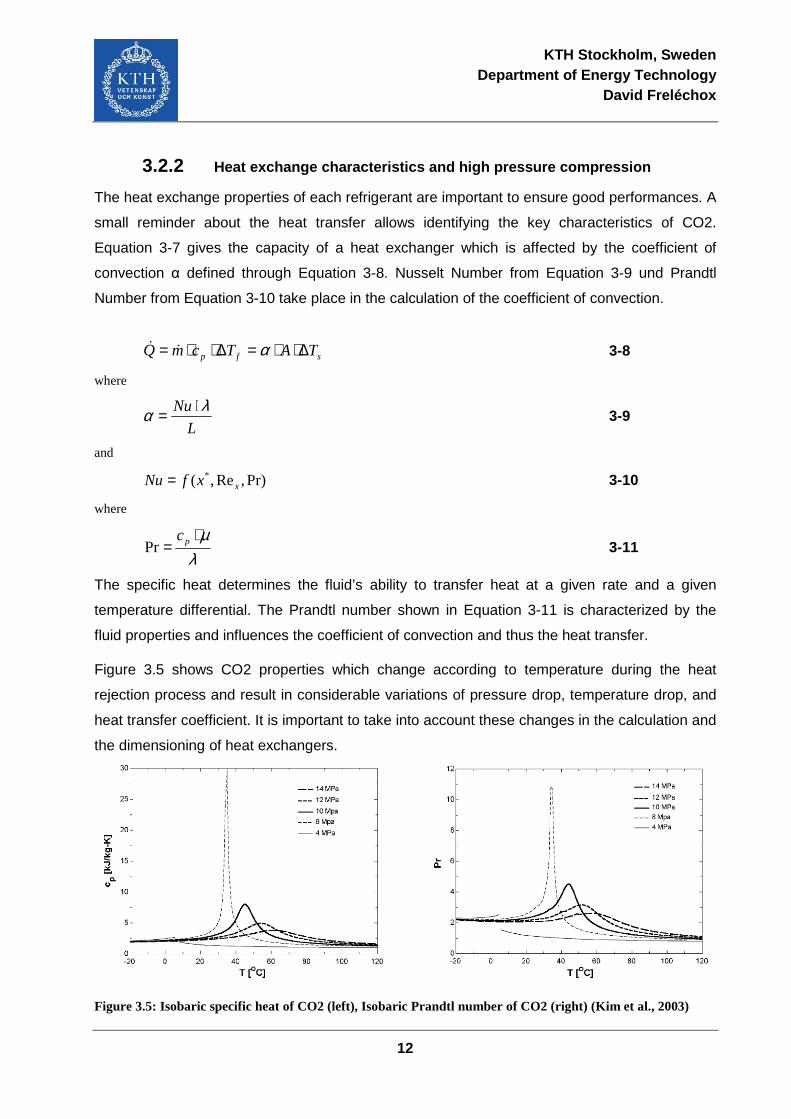
Figure 3.5 shows CO2 properties which change according to temperature during the heat
rejection process and result in considerable variations of pressure drop, temperature drop, and
heat transfer coefficient. It is important to take into account these changes in the calculation and
the dimensioning of heat exchangers.
Figure 3.5: Isobaric specific heat of CO2 (left), Isobaric Prandtl number of CO2 (right) (Kim et al., 2003)
KTH Stockholm, Sweden Department of Energy Technology
David Freléchox
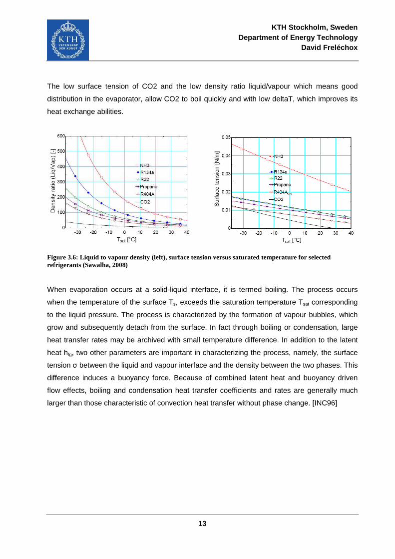
13
The low surface tension of CO2 and the low density ratio liquid/vapour which means good
distribution in the evaporator, allow CO2 to boil quickly and with low deltaT, which improves its
heat exchange abilities.
Figure 3.6: Liquid to vapour density (left), surface tension versus saturated temperature for selected refrigerants (Sawalha, 2008)
When evaporation occurs at a solid-liquid interface, it is termed boiling. The process occurs
when the temperature of the surface Ts, exceeds the saturation temperature Tsat corresponding
to the liquid pressure. The process is characterized by the formation of vapour bubbles, which
grow and subsequently detach from the surface. In fact through boiling or condensation, large
heat transfer rates may be archived with small temperature difference. In addition to the latent
heat hfg, two other parameters are important in characterizing the process, namely, the surface
tension σ between the liquid and vapour interface and the density between the two phases. This
difference induces a buoyancy force. Because of combined latent heat and buoyancy driven
flow effects, boiling and condensation heat transfer coefficients and rates are generally much
larger than those characteristic of convection heat transfer without phase change. [INC96]

KTH Stockholm, Sweden Department of Energy Technology
David Freléchox
14
CO2 compressors generally operate at higher pressures and with a larger pressure differential
than traditional refrigerants; but its pressure ratio is lower. As can be seen in the Figure 3.7, the
piston displacement is 6.7 superior with R134a than with CO2 for the same cooling capacity.
Losses from the re-expansion of the fluid after the compression are also lower with CO2
compressors. Despite the high levels of pressure and the shape of its Pressure-Volume (PV)
diagram, the negative effects of the pressure drop through the valves tend to be lower for CO2
compressors and give them a better efficiency.
Figure 3.7: Compressor pressure diagrams for R134a and CO2 assuming equal cooling capacity (π: pressure ratio, pm: mean effective pressure) (Kim et al., 2003)
3.2.3 Efficiency of CO2 versus synthetic refrigerants
Assuming given evaporating temperature and given minimum heat rejection temperature, the
transcritical cycle suffers from larger thermodynamic losses than an ‘ordinary’ cycle with
condensation. Owing to the higher average temperature of heat rejection, and the larger
throttling loss, the theoretical cycle work for CO2 increases compared to a conventional
refrigerant as R-134a as indicated in the Figure 3.8.
Despite this, for a given heat exchanger and a given coolant temperature, the CO2 gas cooler
output temperature could be less than for a standard cycle. This results of the higher logarithmic
mean temperature difference between the refrigerant and the coolant. Moreover, given the
positive properties of CO2 for heat transfer, the evaporation temperature could generally be
higher with CO2. [KIM03]
KTH Stockholm, Sweden Department of Energy Technology
David Freléchox
15
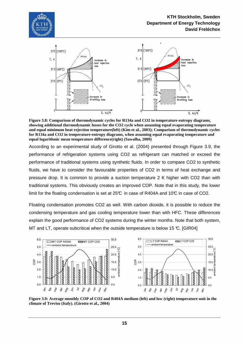
Figure 3.8: Comparison of thermodynamic cycles for R134a and CO2 in temperature-entropy diagrams, showing additional thermodynamic losses for the CO2 cycle when assuming equal evaporating temperature and equal minimum heat rejection temperature(left) (Kim et al., 2003); Comparison of thermodynamic cycles for R134a and CO2 in temperature-entropy diagrams, when assuming equal evaporating temperature and equal logarithmic mean temperature difference(right) (Sawalha, 2009)
According to an experimental study of Girotto et al. (2004) presented through Figure 3.9, the
performance of refrigeration systems using CO2 as refrigerant can matched or exceed the
performance of traditional systems using synthetic fluids. In order to compare CO2 to synthetic
fluids, we have to consider the favourable properties of CO2 in terms of heat exchange and
pressure drop. It is common to provide a suction temperature 2 K higher with CO2 than with
traditional systems. This obviously creates an improved COP. Note that in this study, the lower
limit for the floating condensation is set at 25°C in case of R404A and 10°C in case of CO2.
Floating condensation promotes CO2 as well. With carbon dioxide, it is possible to reduce the
condensing temperature and gas cooling temperature lower than with HFC. These differences
explain the good performance of CO2 systems during the winter months. Note that both system,
MT and LT, operate subcritical when the outside temperature is below 15 °C. [GIR04]
Figure 3.9: Average monthly COP of CO2 and R404A medium (left) and low (right) temperature unit in the climate of Treviso (Italy). (Girotto et al., 2004)
KTH Stockholm, Sweden Department of Energy Technology
David Freléchox
16
In this experimental case, the annual energy’s consumption of the CO2 system is about 10%
higher than the R404A system, for the same cooling capacity. This difference is solely due to
the overconsumption of the MT unit. The LT unit energy consumption is equivalent to that with
R404A. Girotto et al. (2004) suggests that such CO2 systems could reach the annual
performance of traditional systems in cold climates, such as cities of central or north Europe like
Brussels or Stockholm.
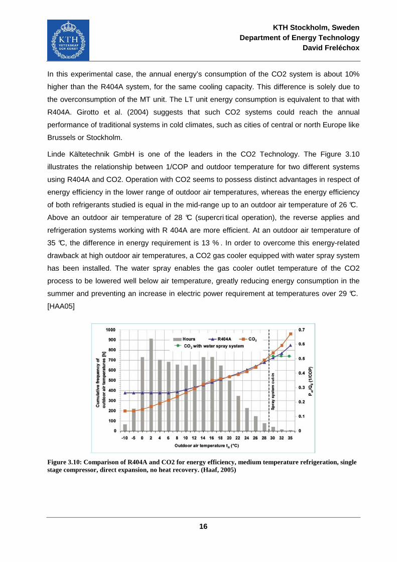
Linde Kältetechnik GmbH is one of the leaders in the CO2 Technology. The Figure 3.10
illustrates the relationship between 1/COP and outdoor temperature for two different systems
using R404A and CO2. Operation with CO2 seems to possess distinct advantages in respect of
energy efficiency in the lower range of outdoor air temperatures, whereas the energy efficiency
of both refrigerants studied is equal in the mid-range up to an outdoor air temperature of 26 °C.
Above an outdoor air temperature of 28 °C (supercri tical operation), the reverse applies and
refrigeration systems working with R 404A are more efficient. At an outdoor air temperature of
35 °C, the difference in energy requirement is 13 % . In order to overcome this energy-related
drawback at high outdoor air temperatures, a CO2 gas cooler equipped with water spray system
has been installed. The water spray enables the gas cooler outlet temperature of the CO2
process to be lowered well below air temperature, greatly reducing energy consumption in the
summer and preventing an increase in electric power requirement at temperatures over 29 °C.
[HAA05]
Figure 3.10: Comparison of R404A and CO2 for energy efficiency, medium temperature refrigeration, single stage compressor, direct expansion, no heat recovery. (Haaf, 2005)
KTH Stockholm, Sweden Department of Energy Technology
David Freléchox
17
3.3 CO2 solutions in supermarket refrigeration
In general, two temperature levels are required in supermarkets for chilled and frozen products.
Product temperatures of around +3°C and –18°C are c ommonly maintained. In these
applications, there are mainly three design options: indirect system, cascade DX system or
transcritical DX system. It is also possible to advantage of different system and built mixed
system. The following section describes CO2-based solutions that fulfil the refrigeration
requirements of supermarkets.
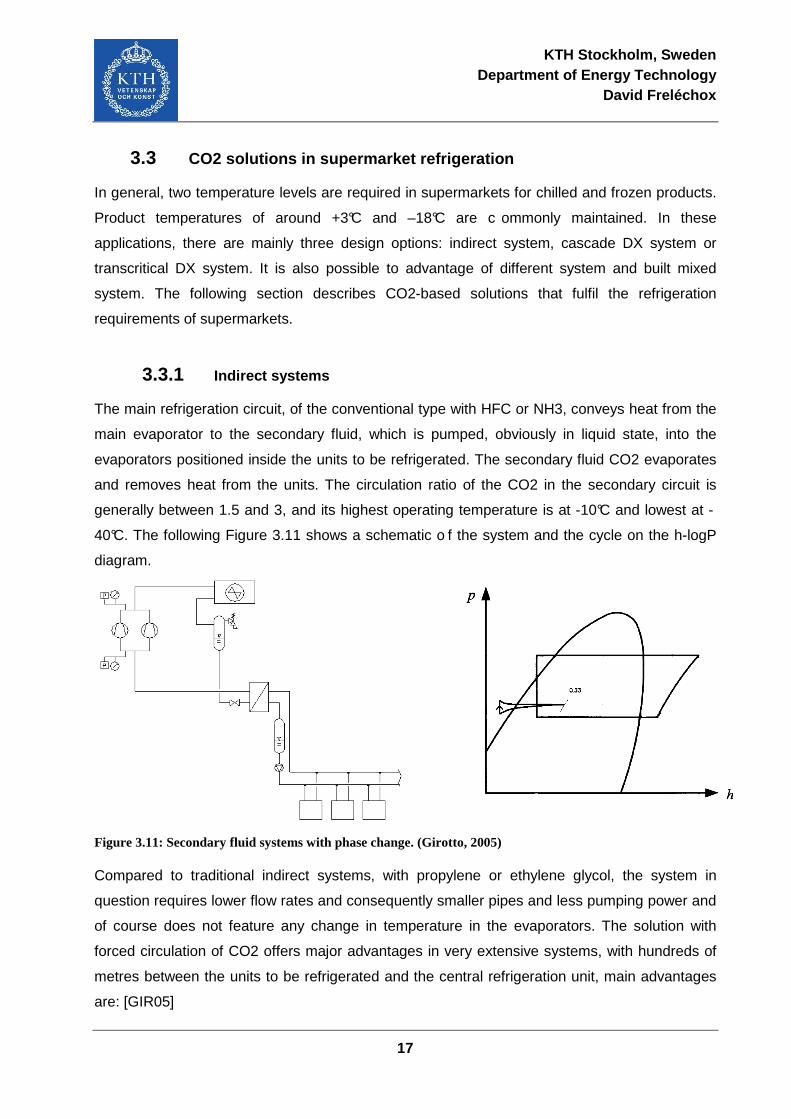
3.3.1 Indirect systems
The main refrigeration circuit, of the conventional type with HFC or NH3, conveys heat from the
main evaporator to the secondary fluid, which is pumped, obviously in liquid state, into the
evaporators positioned inside the units to be refrigerated. The secondary fluid CO2 evaporates
and removes heat from the units. The circulation ratio of the CO2 in the secondary circuit is
generally between 1.5 and 3, and its highest operating temperature is at -10°C and lowest at -
40°C. The following Figure 3.11 shows a schematic o f the system and the cycle on the h-logP
diagram.
Figure 3.11: Secondary fluid systems with phase change. (Girotto, 2005)
Compared to traditional indirect systems, with propylene or ethylene glycol, the system in
question requires lower flow rates and consequently smaller pipes and less pumping power and
of course does not feature any change in temperature in the evaporators. The solution with
forced circulation of CO2 offers major advantages in very extensive systems, with hundreds of
metres between the units to be refrigerated and the central refrigeration unit, main advantages
are: [GIR05]
KTH Stockholm, Sweden Department of Energy Technology
David Freléchox
18
� non-toxic fluid in circulation
� no problem as regards the return of the oil regarding DX systems
� low energy consumption for pumping regarding indirect brine systems
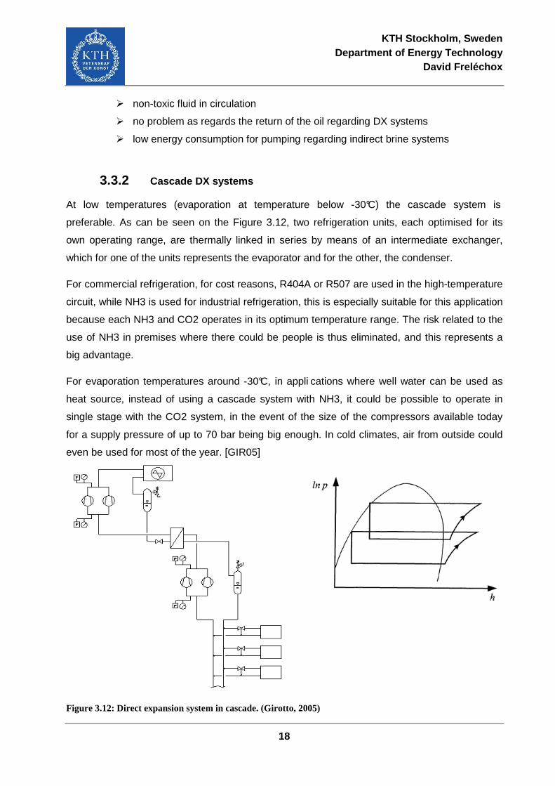
3.3.2 Cascade DX systems
At low temperatures (evaporation at temperature below -30°C) the cascade system is
preferable. As can be seen on the Figure 3.12, two refrigeration units, each optimised for its
own operating range, are thermally linked in series by means of an intermediate exchanger,
which for one of the units represents the evaporator and for the other, the condenser.
For commercial refrigeration, for cost reasons, R404A or R507 are used in the high-temperature
circuit, while NH3 is used for industrial refrigeration, this is especially suitable for this application
because each NH3 and CO2 operates in its optimum temperature range. The risk related to the
use of NH3 in premises where there could be people is thus eliminated, and this represents a
big advantage.
For evaporation temperatures around -30°C, in appli cations where well water can be used as
heat source, instead of using a cascade system with NH3, it could be possible to operate in
single stage with the CO2 system, in the event of the size of the compressors available today
for a supply pressure of up to 70 bar being big enough. In cold climates, air from outside could
even be used for most of the year. [GIR05]
Figure 3.12: Direct expansion system in cascade. (Girotto, 2005)

KTH Stockholm, Sweden Department of Energy Technology
David Freléchox
19
3.3.3 Transcritical DX systems
In this system the CO2 at high pressure rejects heat directly into the air heat exchanger (a
secondary water circuit can naturally be used, but the cost is higher). As can be seen on the
Figure 3.13, the cycle should be supercritical when the condensing temperature is above the
critical point at 31°C. For lower temperatures, the cycle is subcritical.
The fundamental difference between operations in the two conditions lies in the way the high
pressure is controlled. While in subcritical conditions, the high pressure is indirectly set by the
temperature of the cooling fluid. In the case of operation with cooling above critical pressure, a
special control is required, and this can be done through the valve positioned between the
exchanger and the receiver. The control method used must optimise capacity and efficiency.
The efficiency of the standard cycle in supercritical conditions is much below that of the same
cycle with HFC/ HC or NH3, conditions being the same. In cold climates, the system can
operate in subcritical conditions for most of the time. [GIR05]
Figure 3.13: Direct expansion system and transfer of heat directly into the environment. (Girotto, 2005)
KTH Stockholm, Sweden Department of Energy Technology
David Freléchox
20
3.4 Safety issues
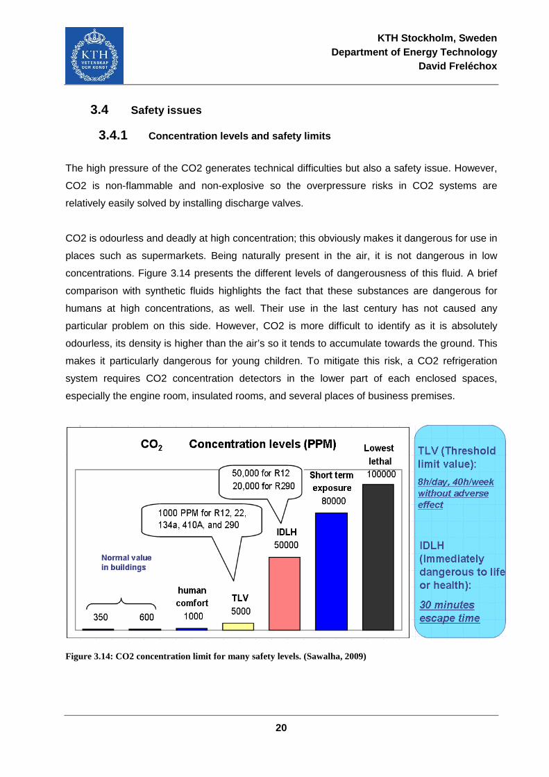
3.4.1 Concentration levels and safety limits
The high pressure of the CO2 generates technical difficulties but also a safety issue. However,
CO2 is non-flammable and non-explosive so the overpressure risks in CO2 systems are
relatively easily solved by installing discharge valves.
CO2 is odourless and deadly at high concentration; this obviously makes it dangerous for use in
places such as supermarkets. Being naturally present in the air, it is not dangerous in low
concentrations. Figure 3.14 presents the different levels of dangerousness of this fluid. A brief
comparison with synthetic fluids highlights the fact that these substances are dangerous for
humans at high concentrations, as well. Their use in the last century has not caused any
particular problem on this side. However, CO2 is more difficult to identify as it is absolutely
odourless, its density is higher than the air’s so it tends to accumulate towards the ground. This
makes it particularly dangerous for young children. To mitigate this risk, a CO2 refrigeration
system requires CO2 concentration detectors in the lower part of each enclosed spaces,
especially the engine room, insulated rooms, and several places of business premises.
Figure 3.14: CO2 concentration limit for many safety levels. (Sawalha, 2009)
KTH Stockholm, Sweden Department of Energy Technology
David Freléchox
21
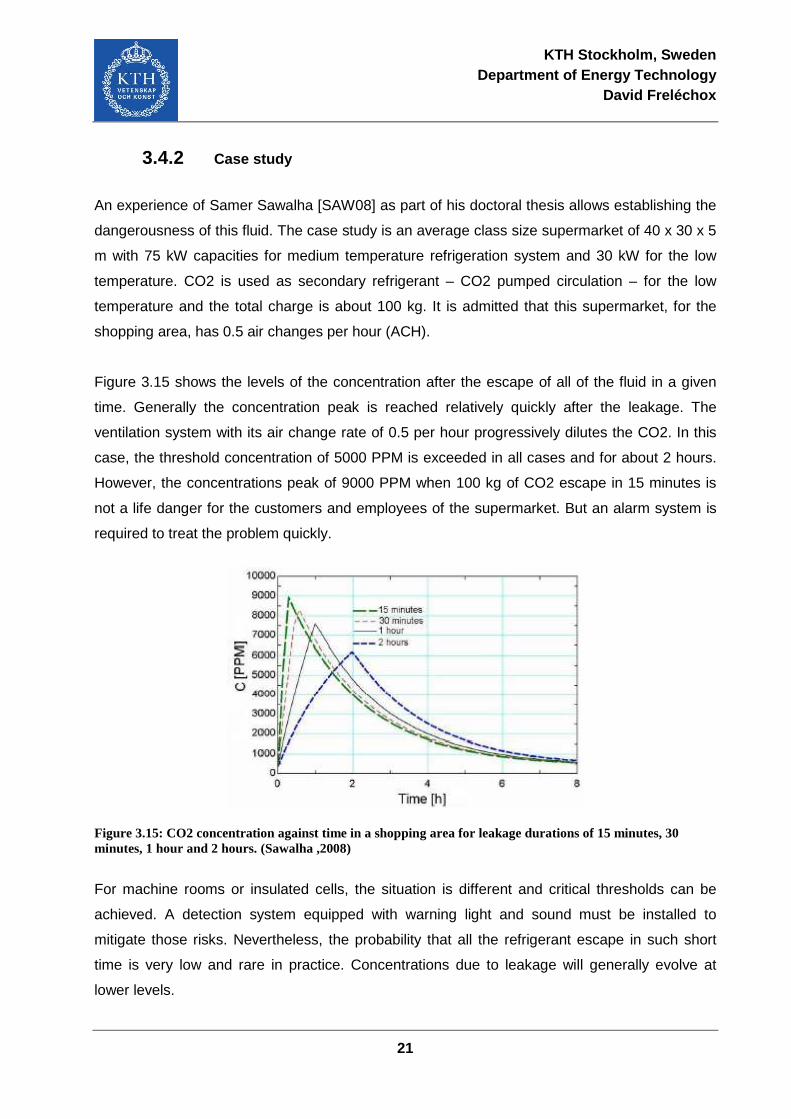
3.4.2 Case study
An experience of Samer Sawalha [SAW08] as part of his doctoral thesis allows establishing the
dangerousness of this fluid. The case study is an average class size supermarket of 40 x 30 x 5
m with 75 kW capacities for medium temperature refrigeration system and 30 kW for the low
temperature. CO2 is used as secondary refrigerant – CO2 pumped circulation – for the low
temperature and the total charge is about 100 kg. It is admitted that this supermarket, for the
shopping area, has 0.5 air changes per hour (ACH).
Figure 3.15 shows the levels of the concentration after the escape of all of the fluid in a given
time. Generally the concentration peak is reached relatively quickly after the leakage. The
ventilation system with its air change rate of 0.5 per hour progressively dilutes the CO2. In this
case, the threshold concentration of 5000 PPM is exceeded in all cases and for about 2 hours.
However, the concentrations peak of 9000 PPM when 100 kg of CO2 escape in 15 minutes is
not a life danger for the customers and employees of the supermarket. But an alarm system is
required to treat the problem quickly.
Figure 3.15: CO2 concentration against time in a shopping area for leakage durations of 15 minutes, 30 minutes, 1 hour and 2 hours. (Sawalha ,2008)
For machine rooms or insulated cells, the situation is different and critical thresholds can be
achieved. A detection system equipped with warning light and sound must be installed to
mitigate those risks. Nevertheless, the probability that all the refrigerant escape in such short
time is very low and rare in practice. Concentrations due to leakage will generally evolve at
lower levels.
KTH Stockholm, Sweden Department of Energy Technology
David Freléchox
22
4 Measurements and Evaluation Methods
The important parameters for the evaluation of cooling systems are mainly the cooling
capacities and the COPs. For these capacities, the temperatures and pressures are needed to
determine the enthalpies and then the mass flow rate is needed in order to determine the
cooling capacities and different losses. Mass flow rate is not measured directly and it is evaluted
from the compressor side. Then COPs are calculated using the cooling capacity and the
measured or calculated electrical consumption.
4.1 Pressure and temperature measurements
The input data for the calculation of the refrigerant thermodynamics states are the measures of
pressure and temperature. The temperature sensor types are generally PT100 or PT1000 and
widely used in the refrigeration regulation. Pressure sensors give an absolute or relative
pressure depending on their initial settings. The sensors used are generally from the
manufacturer Danfoss and types are AKS or HSK according to their pressure range.
The sensors were not installed especially for our study but are primarily used to operate the
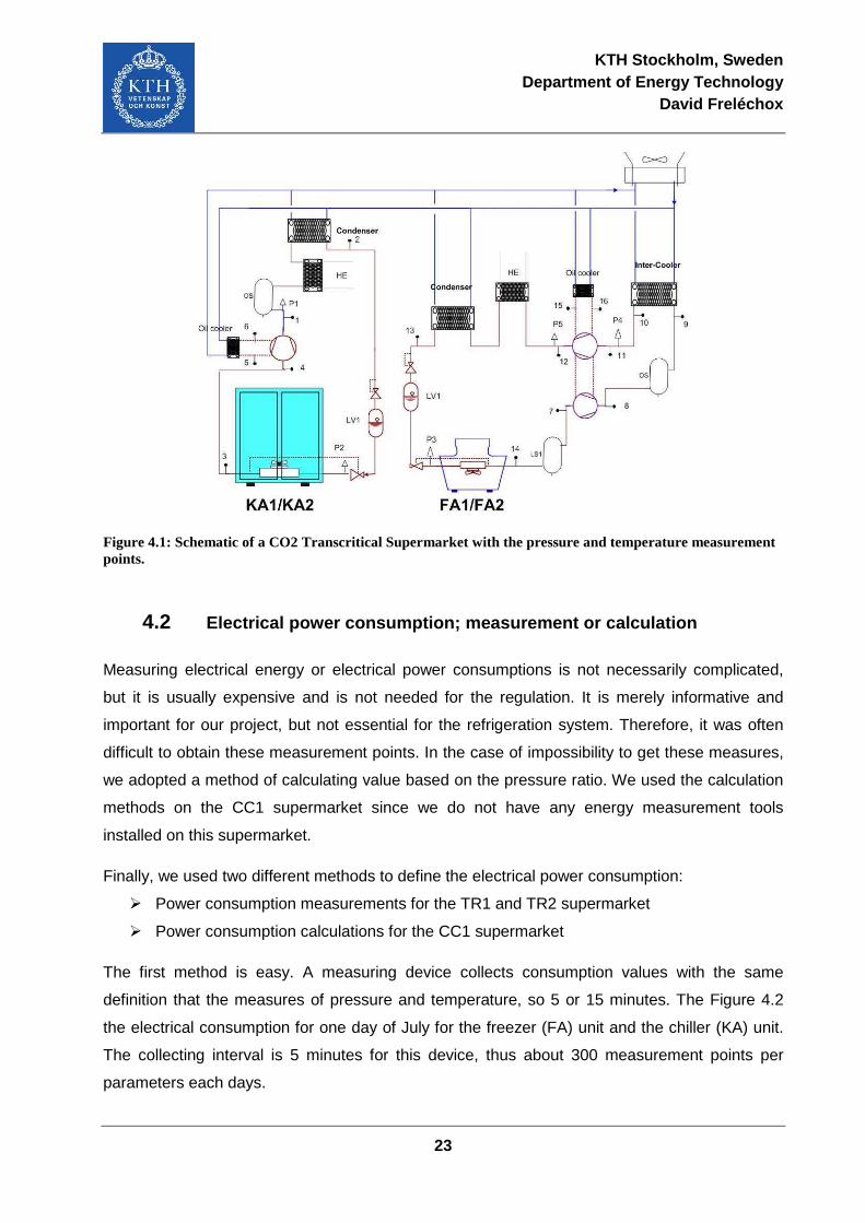
systems and are essential regulation elements. On the Figure 4.1, the measurement points are
shown. These points allow tracing the refrigeration cycle in the h-logP diagram and calculating
the cooling capacity as well as various parameters which could influence this capacity, such as
the internal and external superheat, the subcooling and the pressure ratio.
We used two different systems for the data acquisition:
� -IWMAC with an interval of 5 minutes for TR1 and TR2 supermarket [IWM09]
� -RDM with an interval of 15 minutes for CC1 supermarket [RDM09]
KTH Stockholm, Sweden Department of Energy Technology
David Freléchox
23
Figure 4.1: Schematic of a CO2 Transcritical Supermarket with the pressure and temperature measurement points.
4.2 Electrical power consumption; measurement or calcul ation
Measuring electrical energy or electrical power consumptions is not necessarily complicated,
but it is usually expensive and is not needed for the regulation. It is merely informative and
important for our project, but not essential for the refrigeration system. Therefore, it was often
difficult to obtain these measurement points. In the case of impossibility to get these measures,
we adopted a method of calculating value based on the pressure ratio. We used the calculation
methods on the CC1 supermarket since we do not have any energy measurement tools
installed on this supermarket.
Finally, we used two different methods to define the electrical power consumption:
� Power consumption measurements for the TR1 and TR2 supermarket
� Power consumption calculations for the CC1 supermarket
The first method is easy. A measuring device collects consumption values with the same
definition that the measures of pressure and temperature, so 5 or 15 minutes. The Figure 4.2
the electrical consumption for one day of July for the freezer (FA) unit and the chiller (KA) unit.
The collecting interval is 5 minutes for this device, thus about 300 measurement points per
parameters each days.
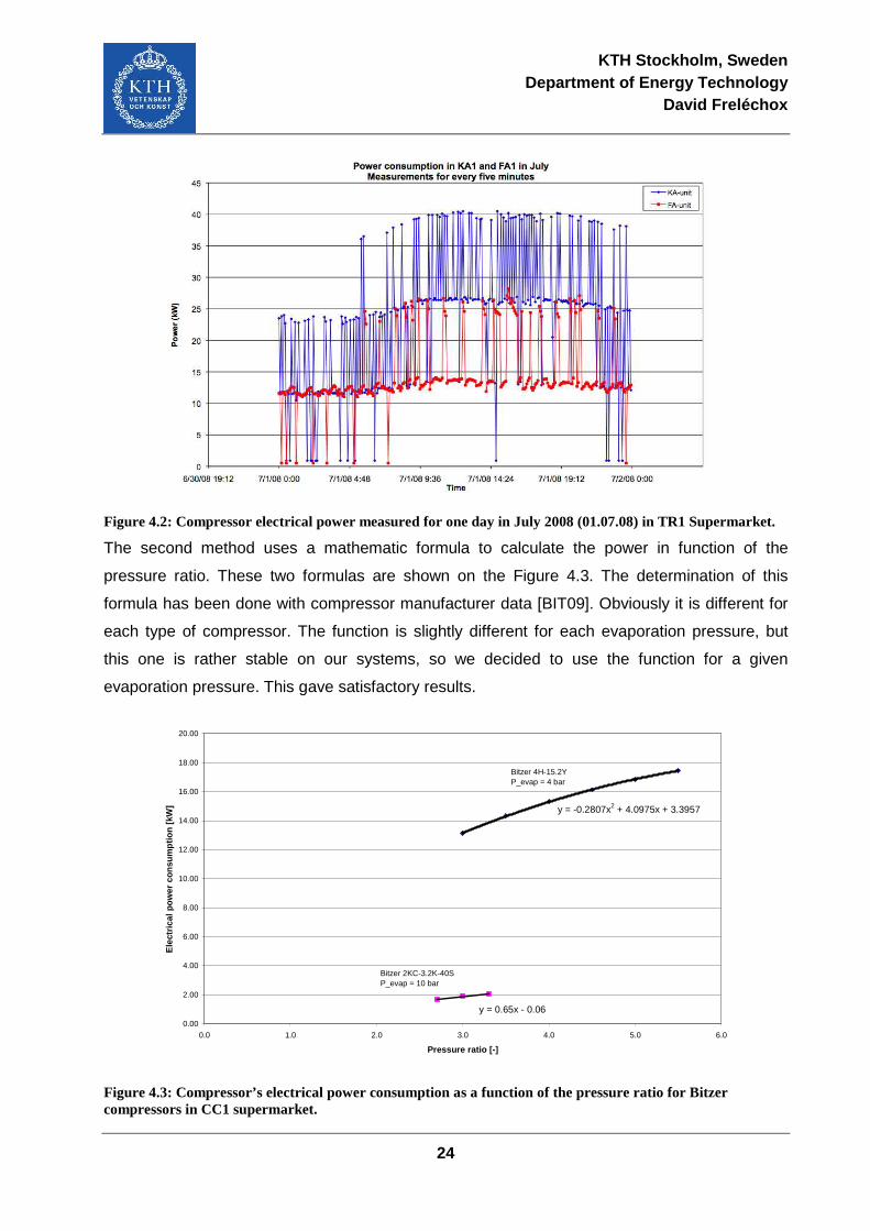
KTH Stockholm, Sweden Department of Energy Technology
David Freléchox
24
Figure 4.2: Compressor electrical power measured for one day in July 2008 (01.07.08) in TR1 Supermarket.
The second method uses a mathematic formula to calculate the power in function of the
pressure ratio. These two formulas are shown on the Figure 4.3. The determination of this
formula has been done with compressor manufacturer data [BIT09]. Obviously it is different for
each type of compressor. The function is slightly different for each evaporation pressure, but
this one is rather stable on our systems, so we decided to use the function for a given
evaporation pressure. This gave satisfactory results.
y = -0.2807x2 + 4.0975x + 3.3957
y = 0.65x - 0.060.00
2.00
4.00
6.00
8.00
10.00
12.00
14.00
16.00
18.00
20.00
0.0 1.0 2.0 3.0 4.0 5.0 6.0
Pressure ratio [-]
Ele
ctric
al p
ower
con
sum
ptio
n [k
W]
Bitzer 4H-15.2YP_evap = 4 bar
Bitzer 2KC-3.2K-40SP_evap = 10 bar
Figure 4.3: Compressor’s electrical power consumption as a function of the pressure ratio for Bitzer compressors in CC1 supermarket.
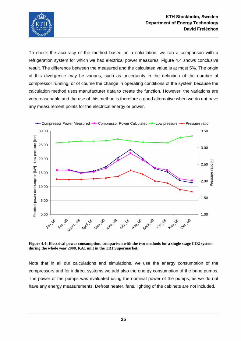
KTH Stockholm, Sweden Department of Energy Technology
David Freléchox
25
To check the accuracy of the method based on a calculation, we ran a comparison with a
refrigeration system for which we had electrical power measures. Figure 4.4 shows conclusive
result. The difference between the measured and the calculated value is at most 5%. The origin
of this divergence may be various, such as uncertainty in the definition of the number of
compressor running, or of course the change in operating conditions of the system because the
calculation method uses manufacturer data to create the function. However, the variations are
very reasonable and the use of this method is therefore a good alternative when we do not have
any measurement points for the electrical energy or power.
0.00
5.00
10.00
15.00
20.00
25.00
30.00
Jan_
08
Feb_0
8
Mar
ch_0
8
April_
08
May
_08
June
_08
July_
08
Aug_0
8
Sept_
08
Oct_08
Nov_0
8
Dec_0
8
Ele
ctric
al p
ower
con
sum
ptio
n [k
W] -
Low
pre
ssur
e [b
ar]
1.00
1.50
2.00
2.50
3.00
3.50
Pre
ssur
e ra
tio [-
]
Compressor Power Measured Compressor Power Calculated Low pressure Pressure ratio
Figure 4.4: Electrical power consumption, comparison with the two methods for a single stage CO2 system during the whole year 2008, KA1 unit in the TR1 Supermarket.
Note that in all our calculations and simulations, we use the energy consumption of the
compressors and for indirect systems we add also the energy consumption of the brine pumps.
The power of the pumps was evaluated using the nominal power of the pumps, as we do not
have any energy measurements. Defrost heater, fans, lighting of the cabinets are not included.
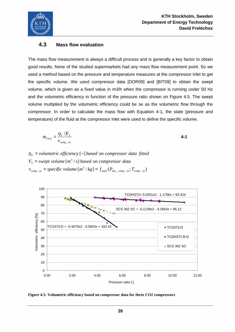
KTH Stockholm, Sweden Department of Energy Technology
David Freléchox
26
4.3 Mass flow evaluation
The mass flow measurement is always a difficult process and is generally a key factor to obtain
good results. None of the studied supermarkets had any mass flow measurement point. So we
used a method based on the pressure and temperature measures at the compressor inlet to get
the specific volume. We used compressor data [DOR09] and [BIT09] to obtain the swept
volume, which is given as a fixed value in m3/h when the compressor is running under 50 Hz
and the volumetric efficiency in function of the pressure ratio shown on Figure 4.5. The swept
volume multiplied by the volumetric efficiency could be se as the volumetric flow through the
compressor. In order to calculate the mass flow with Equation 4-1, the state (pressure and
temperature) of the fluid at the compressor inlet were used to define the specific volume.
incomp
SVCO v
Vm
_2
&
&⋅
=η
4-1
);(]/[
]/[
][
___3
_
3
incompincompabsstateincomp
S
V
TPfkgmvolumespecificv
datacompressoronbasedsmvolumesweptV
fitteddatacompressoronbasedefficiencyvolumetric
==
=
−=&
η
TCS373-D = -0.4079x2 - 6.5843x + 102.42
TCDH372= 0.0251x2 - 1.1706x + 93.424
SCS 362 SC = -0,1139x2 - 4,1854x + 95,12
0
10
20
30
40
50
60
70
80
90
100
0.00 2.00 4.00 6.00 8.00 10.00 12.00
Pressure ratio [-]
Vol
umet
ric e
ffici
ency
[%]
TCS373-D
TCDH372 B-D
SCS 362 SC
Figure 4.5: Volumetric efficiency based on compressor data for three CO2 compressors
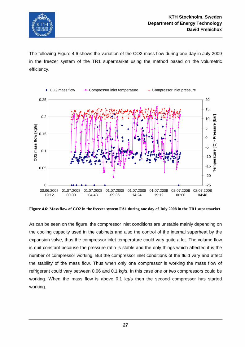
KTH Stockholm, Sweden Department of Energy Technology
David Freléchox
27
The following Figure 4.6 shows the variation of the CO2 mass flow during one day in July 2009
in the freezer system of the TR1 supermarket using the method based on the volumetric
efficiency.
0
0.05
0.1
0.15
0.2
0.25
30.06.200819:12
01.07.200800:00
01.07.200804:48
01.07.200809:36
01.07.200814:24
01.07.200819:12
02.07.200800:00
02.07.200804:48
CO
2 m
ass
flow
[kg/
s]
-25
-20
-15
-10
-5
0
5
10
15
20
Tem
pera
ture
[°C
] - P
ress
ure
[bar
]
CO2 mass flow Compressor inlet temperature Compressor inlet pressure
Figure 4.6: Mass flow of CO2 in the freezer system FA1 during one day of July 2008 in the TR1 supermarket
As can be seen on the figure, the compressor inlet conditions are unstable mainly depending on
the cooling capacity used in the cabinets and also the control of the internal superheat by the
expansion valve, thus the compressor inlet temperature could vary quite a lot. The volume flow
is quit constant because the pressure ratio is stable and the only things which affected it is the
number of compressor working. But the compressor inlet conditions of the fluid vary and affect
the stability of the mass flow. Thus when only one compressor is working the mass flow of
refrigerant could vary between 0.06 and 0.1 kg/s. In this case one or two compressors could be
working. When the mass flow is above 0.1 kg/s then the second compressor has started
working.
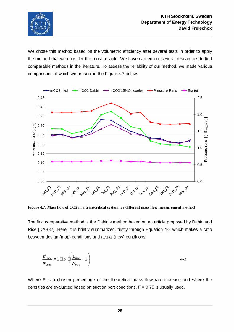
KTH Stockholm, Sweden Department of Energy Technology
David Freléchox
28
We chose this method based on the volumetric efficiency after several tests in order to apply
the method that we consider the most reliable. We have carried out several researches to find
comparable methods in the literature. To assess the reliability of our method, we made various
comparisons of which we present in the Figure 4.7 below.
0.00
0.05
0.10
0.15
0.20
0.25
0.30
0.35
0.40
0.45
Jan_
08
Feb_0
8
Mar
_08
Apr_0
8
May
_08
Jun_
08
Jul_0
8
Aug_0
8
Sep_0
8
Oct_08
Nov_0
8
Dec_0
8
Jan_
09
Feb_0
9
Mar
_09
Mas
s flo
w C
O2
[kg/
s]
0.0
0.5
1.0
1.5
2.0
2.5
Pre
ssur
e ra
tio [
-], E
ta_t
ot [-
]
mCO2 ηvol mCO2 Dabiri mCO2 15%Oil cooler Pressure Ratio Eta tot
Figure 4.7: Mass flow of CO2 in a transcritical system for different mass flow measurement method
The first comparative method is the Dabiri’s method based on an article proposed by Dabiri and
Rice [DAB82]. Here, it is briefly summarized, firstly through Equation 4-2 which makes a ratio
between design (map) conditions and actual (new) conditions:
−⋅+= 11
map
new
map
new Fm
m
ρρ
&
& 4-2
Where F is a chosen percentage of the theoretical mass flow rate increase and where the
densities are evaluated based on suction port conditions. F = 0.75 is usually used.
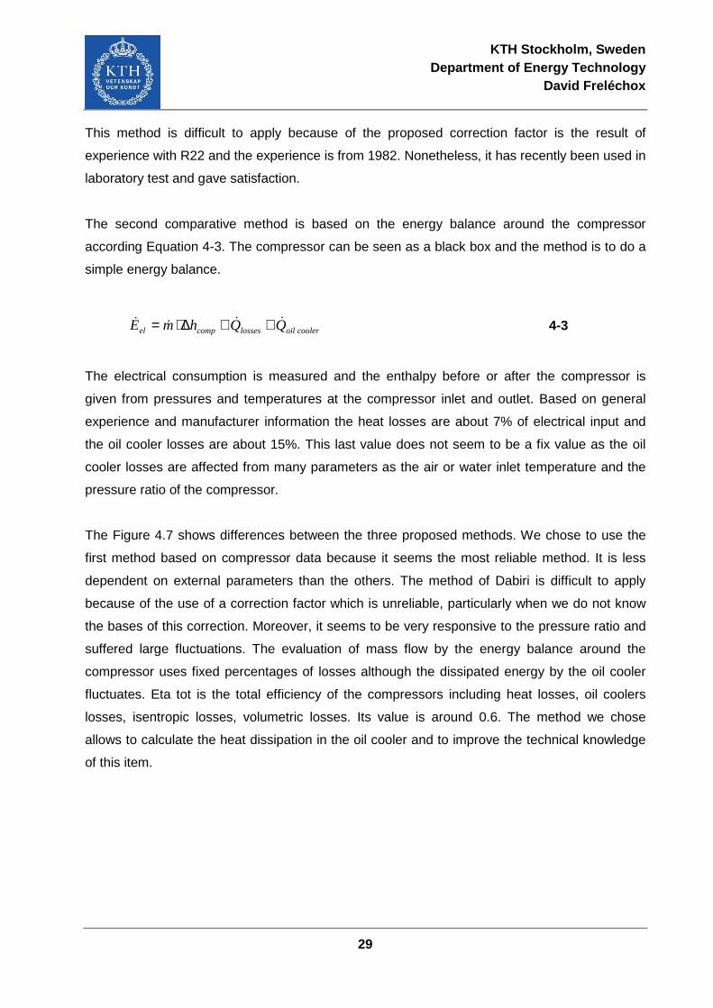
KTH Stockholm, Sweden Department of Energy Technology
David Freléchox
29
This method is difficult to apply because of the proposed correction factor is the result of
experience with R22 and the experience is from 1982. Nonetheless, it has recently been used in
laboratory test and gave satisfaction.
The second comparative method is based on the energy balance around the compressor
according Equation 4-3. The compressor can be seen as a black box and the method is to do a
simple energy balance.
cooleroillossescompel QQhmE &&&& ++∆⋅= 4-3
The electrical consumption is measured and the enthalpy before or after the compressor is
given from pressures and temperatures at the compressor inlet and outlet. Based on general
experience and manufacturer information the heat losses are about 7% of electrical input and
the oil cooler losses are about 15%. This last value does not seem to be a fix value as the oil
cooler losses are affected from many parameters as the air or water inlet temperature and the
pressure ratio of the compressor.
The Figure 4.7 shows differences between the three proposed methods. We chose to use the
first method based on compressor data because it seems the most reliable method. It is less
dependent on external parameters than the others. The method of Dabiri is difficult to apply
because of the use of a correction factor which is unreliable, particularly when we do not know
the bases of this correction. Moreover, it seems to be very responsive to the pressure ratio and
suffered large fluctuations. The evaluation of mass flow by the energy balance around the
compressor uses fixed percentages of losses although the dissipated energy by the oil cooler
fluctuates. Eta tot is the total efficiency of the compressors including heat losses, oil coolers
losses, isentropic losses, volumetric losses. Its value is around 0.6. The method we chose
allows to calculate the heat dissipation in the oil cooler and to improve the technical knowledge
of this item.
KTH Stockholm, Sweden Department of Energy Technology
David Freléchox
30
The Figure 4.8 below gives an overview of the effects of these various methods on our final
objective, the COP calculation. Again, our method based on the volumetric efficiency, COPηvol,
gives satisfactory results. It correlates very well with the COP resulting from the use of losses of
15% through the oil cooler, as well. In contrast, the method proposed by Dabiri and Rice seems
doubtful. Indeed, we do not notice a real correlation with the pressure ratio while we know its
importance on the efficiency of a system. The decrease of the pressure ratio in November 2008
does not really increase the COP which is unlikely.
0.0
1.0
2.0
3.0
4.0
5.0
6.0
Jan_
08
Feb_0
8
Mar
_08
Apr_0
8
May
_08
Jun_
08
Jul_0
8
Aug_0
8
Sep_0
8
Oct_08
Nov_0
8
Dec_0
8
Jan_
09
Feb_0
9
Mar
_09
CO
P [-
], P
R [-
]
COP ηvol COP Dabiri COP 15%oil cooler Pressure Ratio
Figure 4.8:COP of a CO2 transcritical system for different mass flow measurement method
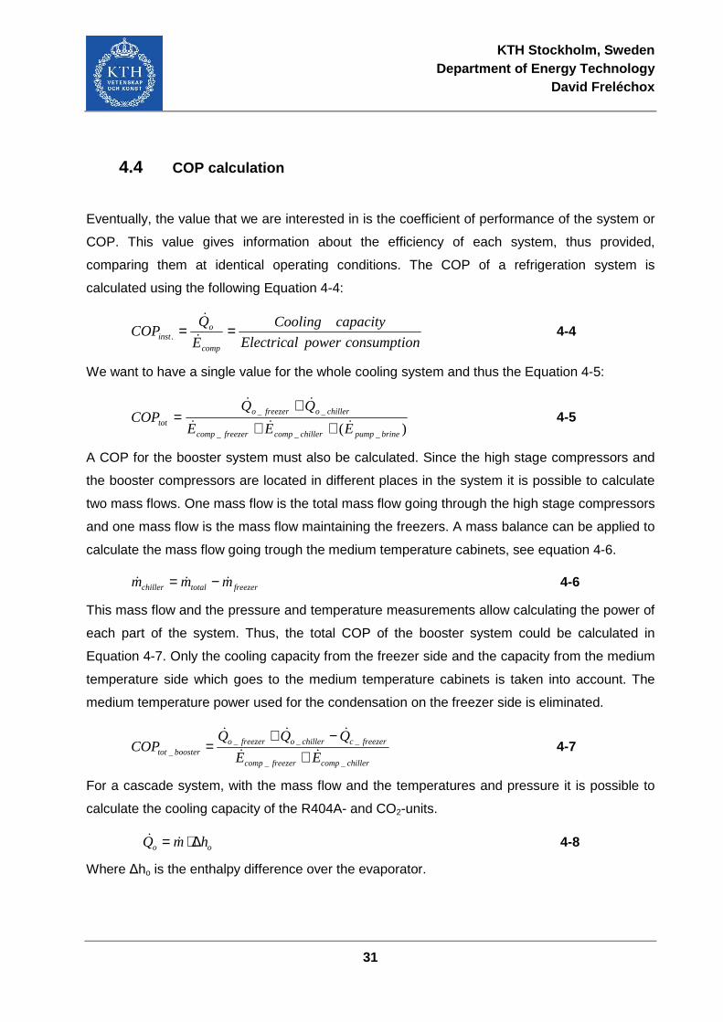
KTH Stockholm, Sweden Department of Energy Technology
David Freléchox
31
4.4 COP calculation
Eventually, the value that we are interested in is the coefficient of performance of the system or
COP. This value gives information about the efficiency of each system, thus provided,
comparing them at identical operating conditions. The COP of a refrigeration system is
calculated using the following Equation 4-4:
nconsumptiopowerElectrical
capacityCooling
E
QCOP
comp
oinst ==
&
&
. 4-4
We want to have a single value for the whole cooling system and thus the Equation 4-5:
)( ___
__
brinepumpchillercompfreezercomp
chillerofreezerotot EEE
QQCOP
&&&
&&
+++
= 4-5
A COP for the booster system must also be calculated. Since the high stage compressors and
the booster compressors are located in different places in the system it is possible to calculate
two mass flows. One mass flow is the total mass flow going through the high stage compressors
and one mass flow is the mass flow maintaining the freezers. A mass balance can be applied to
calculate the mass flow going trough the medium temperature cabinets, see equation 4-6.
freezertotalchiller mmm &&& −=
4-6
This mass flow and the pressure and temperature measurements allow calculating the power of
each part of the system. Thus, the total COP of the booster system could be calculated in
Equation 4-7. Only the cooling capacity from the freezer side and the capacity from the medium
temperature side which goes to the medium temperature cabinets is taken into account. The
medium temperature power used for the condensation on the freezer side is eliminated.
chillercompfreezercomp
freezercchillerofreezeroboostertot EE
QQQCOP
__
____ &&
&&&
+−+
= 4-7
For a cascade system, with the mass flow and the temperatures and pressure it is possible to
calculate the cooling capacity of the R404A- and CO2-units.
oo hmQ ∆⋅= &&
4-8
Where ∆ho is the enthalpy difference over the evaporator.
KTH Stockholm, Sweden Department of Energy Technology
David Freléchox
32
The condenser load of the CO2-unit can be calculated with Equation 4-9.
shaftfreezercompfreezerofreezerc EQQ ____&&& +=
4-9
To decide the load of the medium temperature side cabinets Equation 4-10 are used.
freezercchillerocabo QQQ ___&&& −=
4-10
The electrical energy from the chiller which goes to the freezer can be calculated by Equation 4-11.
chillercompchillero
freezercfreezerforchiller E
Q
QE _
_
_ &&
&& ⋅=−− 4-11
The COP for the freezers can be calculated by Equation 4-12.
freezerpumpsfreezerforchillerfreezercomp
freezerofreezer EEE
QCOP
__
_
&&&
&
++=
−−
4-12
The COP for the chillers can be calculated by Equation 4-13.
cabpumpsfreezerforchillerchillercomp
cabochiller EEE
QCOP
__
_
&&&
&
+−=
−−
4-13
Where opumps QE && ⋅= %4 [GRA07]
To compare the concepts between them, the load ratio has to be identical, i.e. the ratio of the
cooling capacity between the chiller and the freezer is the same for each installation. An
approximate value for European supermarket is 3, so 3 times more cooling capacity for medium
temperature cabinets than for low temperature cabinets. In order to correct our COP according
to a fix load ratio (LRcorr), we developed the Equation 4-14. It is possible to see the
demonstration in the Appendix 1. The abbreviation of load ratio is LR, thus COPtot_LR is the
total COP of system with a defined load ratio LRcorr.
chillercompfreezero
chillerofreezercomp
corr
corr
corrchillero
LRtot
EQ
QE
LR
LR
LRQ
COP
__
__
_
_1
1
&&
&&
&
⋅+⋅
+⋅= 4-14
Note that the COP is the instantaneous efficiency of the installation. We calculated it for each
measurement interval (5 or 15 minutes). Then we did an average to get a monthly value. It may
slightly differ from the monthly COP which is a ratio of energy rather than power.
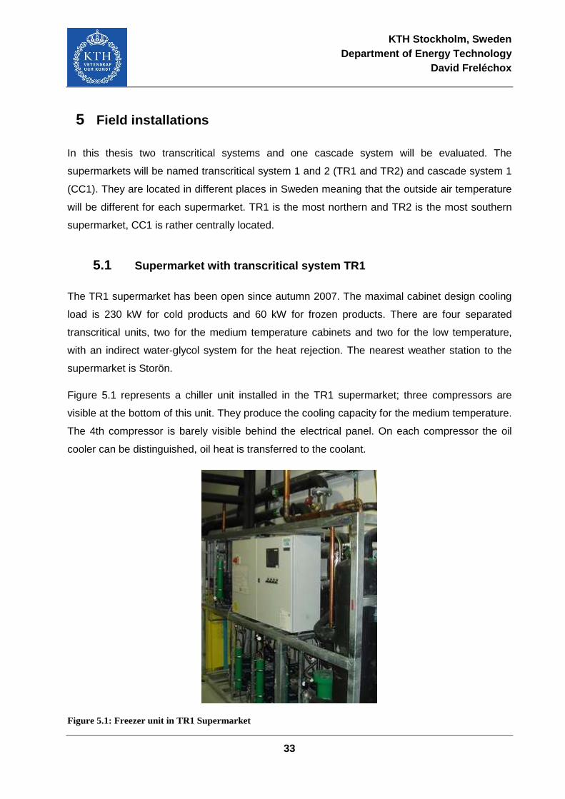
KTH Stockholm, Sweden Department of Energy Technology
David Freléchox
33
5 Field installations
In this thesis two transcritical systems and one cascade system will be evaluated. The
supermarkets will be named transcritical system 1 and 2 (TR1 and TR2) and cascade system 1
(CC1). They are located in different places in Sweden meaning that the outside air temperature
will be different for each supermarket. TR1 is the most northern and TR2 is the most southern
supermarket, CC1 is rather centrally located.
5.1 Supermarket with transcritical system TR1
The TR1 supermarket has been open since autumn 2007. The maximal cabinet design cooling
load is 230 kW for cold products and 60 kW for frozen products. There are four separated
transcritical units, two for the medium temperature cabinets and two for the low temperature,
with an indirect water-glycol system for the heat rejection. The nearest weather station to the
supermarket is Storön.
Figure 5.1 represents a chiller unit installed in the TR1 supermarket; three compressors are
visible at the bottom of this unit. They produce the cooling capacity for the medium temperature.
The 4th compressor is barely visible behind the electrical panel. On each compressor the oil
cooler can be distinguished, oil heat is transferred to the coolant.
Figure 5.1: Freezer unit in TR1 Supermarket
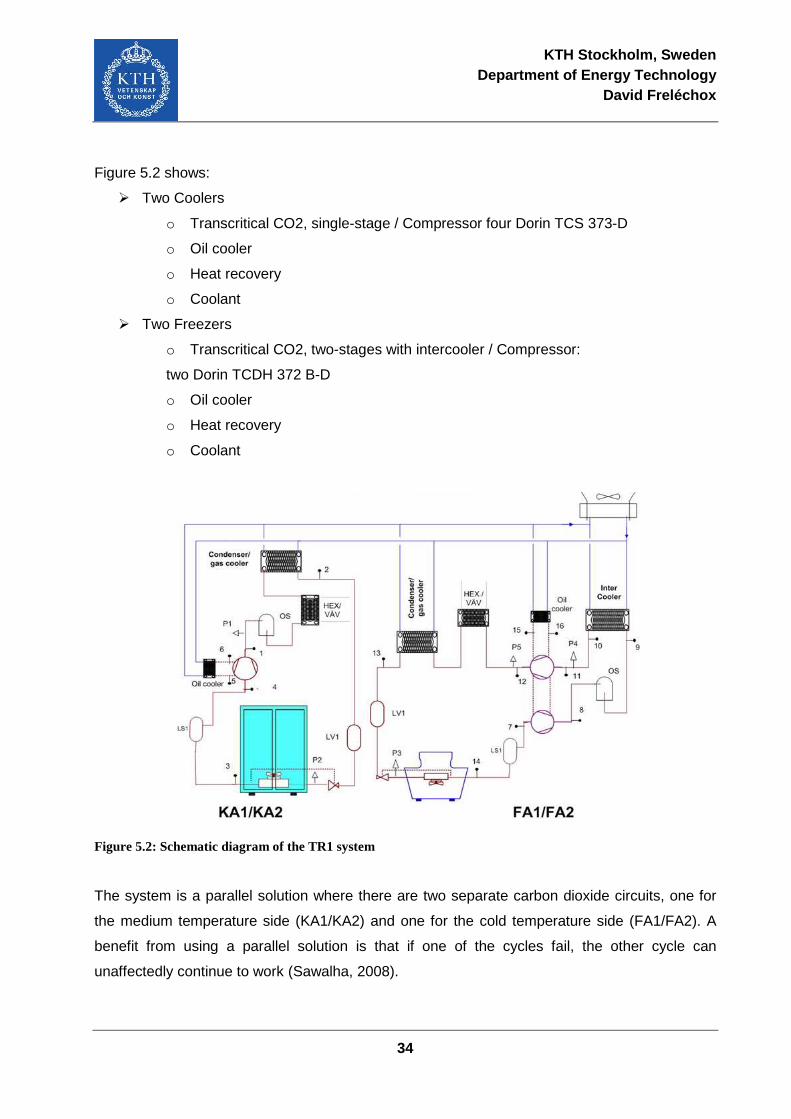
KTH Stockholm, Sweden Department of Energy Technology
David Freléchox
34
Figure 5.2 shows:
� Two Coolers
o Transcritical CO2, single-stage / Compressor four Dorin TCS 373-D
o Oil cooler
o Heat recovery
o Coolant
� Two Freezers
o Transcritical CO2, two-stages with intercooler / Compressor:
two Dorin TCDH 372 B-D
o Oil cooler
o Heat recovery
o Coolant
Figure 5.2: Schematic diagram of the TR1 system
The system is a parallel solution where there are two separate carbon dioxide circuits, one for
the medium temperature side (KA1/KA2) and one for the cold temperature side (FA1/FA2). A
benefit from using a parallel solution is that if one of the cycles fail, the other cycle can
unaffectedly continue to work (Sawalha, 2008).
KTH Stockholm, Sweden Department of Energy Technology
David Freléchox
35
The cold temperature side, seen to the right in Figure 5.2, has a two-stage compression with an
intercooler in between. This is arranged to achieve cold temperatures but still keep low pressure
ratios in the compressors. This will lower the inlet temperature to the second compressor,
decrease the discharge pressure after the second stage and decrease the losses, thereby
increase the efficiency of the system. The carbon dioxide is condensed in the condenser and
expanded in the expansion valve before entering the evaporator (freezers). The expansion
valves are placed out in the supermarkets close to the evaporators. The reason is to minimize
the losses in the system by transporting the refrigerant with high pressure. After the freezer the
refrigerant return to the machinery room and enters a liquid separator (LS) before the
compressors. This is done to make sure that no liquid is going in to the compressors. There are
two units for the cold temperature side (FA1 and FA2). Each unit has two two-stage
compressors.
The medium temperature side has a one-stage compressor since it doesn’t need to operate
with as high pressure ratio as the cold temperature side to maintain the chillers. After the
condenser the refrigerant is expanded in the expansion valve where the pressure is reduced,
before entering the evaporator (chillers). For the same reasons as in the FA-units, the
expansion valves are placed in the Supermarket area close to the cabinets. There are two units
for the medium temperature side (KA1 and KA2). There are four one-stage compressors in
every unit.
The refrigerant in both cycles is gas cooled by a brine circulating between the main condenser
and the two CO2-cycles. The cold brine is used for the oil coolers and the condensers/gas
coolers in both circuits and for the intercooler in the cold temperature side, see Figure 5.2. The
brine condenser is placed on the roof and is using the outside air temperature to cool down the
brine. There is an additional heat exchanger in the brine circuit, placed before the condenser,
for maintaining a heat pump that is supplying the supermarket with air conditioning and heating.
[JOH09]
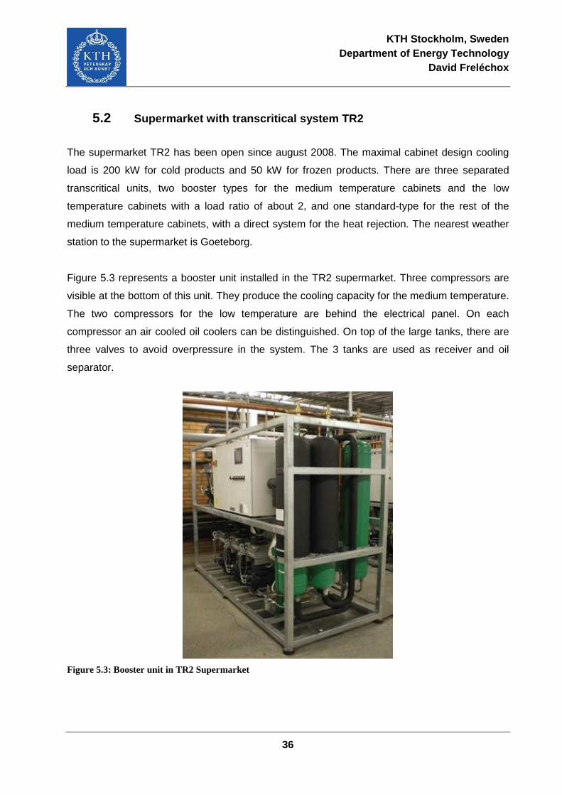
KTH Stockholm, Sweden Department of Energy Technology
David Freléchox
36
5.2 Supermarket with transcritical system TR2
The supermarket TR2 has been open since august 2008. The maximal cabinet design cooling
load is 200 kW for cold products and 50 kW for frozen products. There are three separated
transcritical units, two booster types for the medium temperature cabinets and the low
temperature cabinets with a load ratio of about 2, and one standard-type for the rest of the
medium temperature cabinets, with a direct system for the heat rejection. The nearest weather
station to the supermarket is Goeteborg.
Figure 5.3 represents a booster unit installed in the TR2 supermarket. Three compressors are
visible at the bottom of this unit. They produce the cooling capacity for the medium temperature.
The two compressors for the low temperature are behind the electrical panel. On each
compressor an air cooled oil coolers can be distinguished. On top of the large tanks, there are
three valves to avoid overpressure in the system. The 3 tanks are used as receiver and oil
separator.
Figure 5.3: Booster unit in TR2 Supermarket
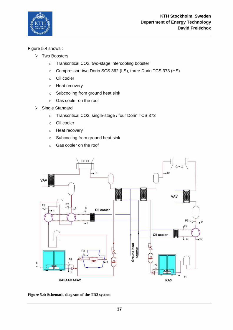
KTH Stockholm, Sweden Department of Energy Technology
David Freléchox
37
Figure 5.4 shows :
� Two Boosters
o Transcritical CO2, two-stage intercooling booster
o Compressor: two Dorin SCS 362 (LS), three Dorin TCS 373 (HS)
o Oil cooler
o Heat recovery
o Subcooling from ground heat sink
o Gas cooler on the roof
� Single Standard
o Transcritical CO2, single-stage / four Dorin TCS 373
o Oil cooler
o Heat recovery
o Subcooling from ground heat sink
o Gas cooler on the roof
Figure 5.4: Schematic diagram of the TR2 system

KTH Stockholm, Sweden Department of Energy Technology
David Freléchox
38
In this supermarket there are one circuit for the medium temperature side (KA3) and one circuit
for a combined medium and cold temperature side (KAFA1/KAFA2). There are two units for the
combined side (KAFA1 and KAFA2) and one unit for only medium temperature cabinets (KA3).
The KA3 cycle can be seen to the right in figure 5.4 and is similar to the KA-unit in trans-critical
system 1. After the evaporator (chillers) the refrigerant enters the one-stage compressor. An
extra heat exchanger is placed after the compressor to recover heat to floor and space heating
of the supermarket. The refrigerant is after that gas cooled/condensed in the gas cooler. The
gas cooler is placed on the roof and uses the outside air temperature to cool down the
refrigerant. Before the refrigerant reaches the expansion valve an extra heat exchanger is
placed to further cool down the refrigerant and gain some additional heat recovery. This heat
exchanger uses a ground heat source for heat exchange with the carbon dioxide.
The combined circuit (KAFA1/KAFA2) side can be seen to the left in figure 5.4 and it serves
both medium temperature cabinets and freezers. The gas cooler is placed on the roof and uses
the outside air to cool down the refrigerant. After the gas cooler/condenser the CO2 runs
through an additional heat exchanger for heat recovery, which also uses the same ground heat
source as in KA3. The ground heat source is used for heating the supermarket. The mass flow
of the refrigerant is separated before it reaches the expansion valves and cabinets/freezers.
After the freezers two compressors called “booster compressors” are located. They increase the
pressure of CO2 to the same pressure as the CO2 has during the evaporation in the medium
temperature cabinets. The mass flows from the medium temperature cabinets and from the
freezers are mixed in the liquid separator before the high stage compressors. The high stage
compressors raise the pressure of the CO2 to condensing pressure. The refrigerant runs
through an additional heat exchanger, for floor and space heating as in the case of KA3-unit,
before it is gas cooled/condensed in the gas cooler. [JOH09]
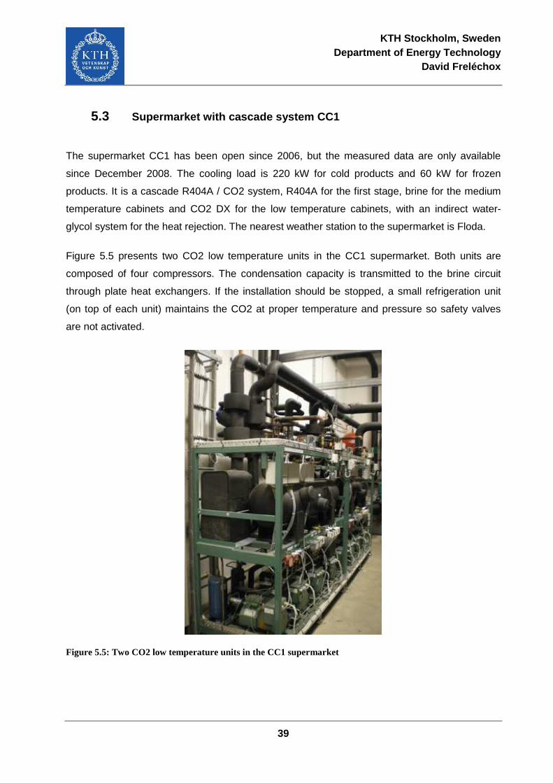
KTH Stockholm, Sweden Department of Energy Technology
David Freléchox
39
5.3 Supermarket with cascade system CC1
The supermarket CC1 has been open since 2006, but the measured data are only available
since December 2008. The cooling load is 220 kW for cold products and 60 kW for frozen
products. It is a cascade R404A / CO2 system, R404A for the first stage, brine for the medium
temperature cabinets and CO2 DX for the low temperature cabinets, with an indirect water-
glycol system for the heat rejection. The nearest weather station to the supermarket is Floda.
Figure 5.5 presents two CO2 low temperature units in the CC1 supermarket. Both units are
composed of four compressors. The condensation capacity is transmitted to the brine circuit
through plate heat exchangers. If the installation should be stopped, a small refrigeration unit
(on top of each unit) maintains the CO2 at proper temperature and pressure so safety valves
are not activated.
Figure 5.5: Two CO2 low temperature units in the CC1 supermarket
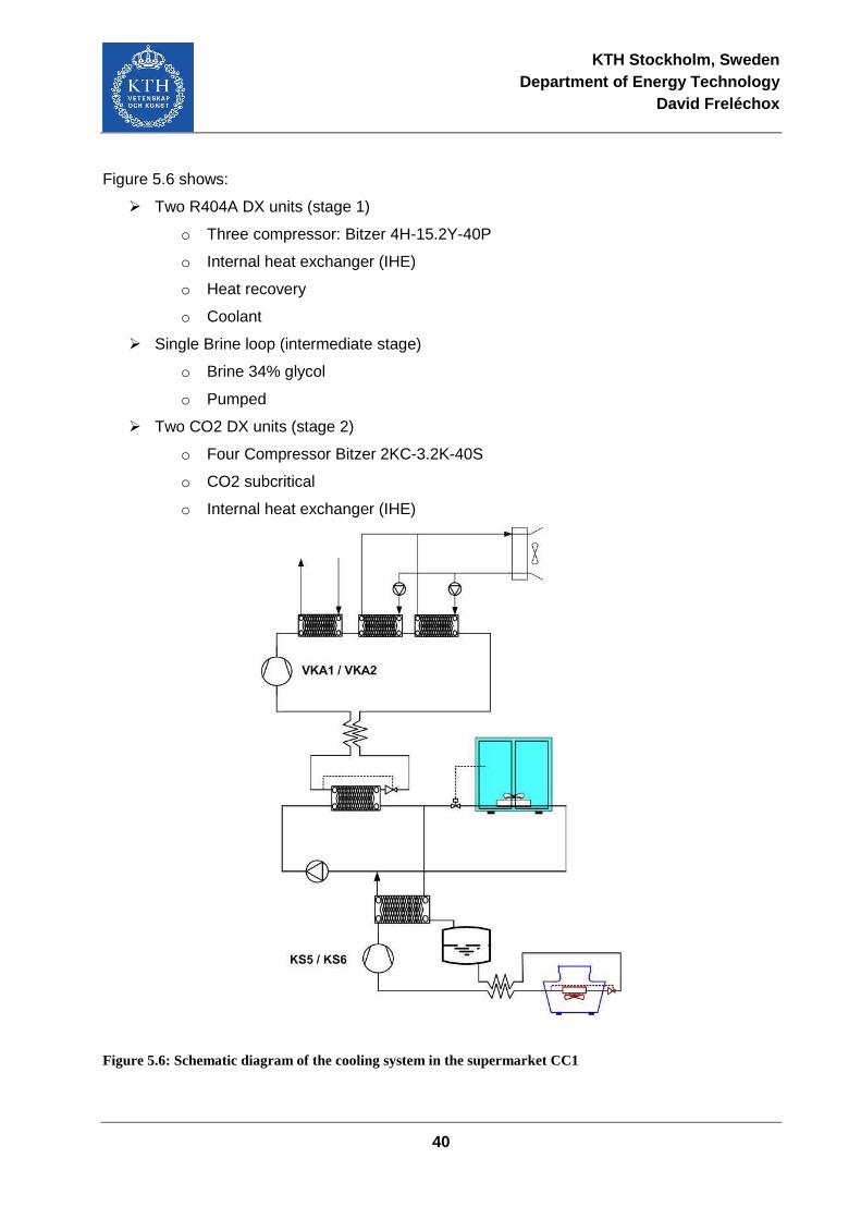
KTH Stockholm, Sweden Department of Energy Technology
David Freléchox
40
Figure 5.6 shows:
� Two R404A DX units (stage 1)
o Three compressor: Bitzer 4H-15.2Y-40P
o Internal heat exchanger (IHE)
o Heat recovery
o Coolant
� Single Brine loop (intermediate stage)
o Brine 34% glycol
o Pumped
� Two CO2 DX units (stage 2)
o Four Compressor Bitzer 2KC-3.2K-40S
o CO2 subcritical
o Internal heat exchanger (IHE)
Figure 5.6: Schematic diagram of the cooling system in the supermarket CC1
KTH Stockholm, Sweden Department of Energy Technology
David Freléchox
41
The system solution is a cascade solution with R404A in the high stage and CO2 in the low
stage. There is direct expansion with CO2 for the freezers and indirect for the chillers. Figure 5.6
shows a schematic picture of the system. There are two units of the low stage (KS5 and KS6)
and two units for the high stage (VKA1 and VKA2). There is only one brine circuit.
R404A in the high stage are condensed by a coolant that is heat exchanging with the outside
air. Before the condenser a desuperheater are located for reuse some of the heat after the
compressor. A subcooler, using the coolant, is placed after the condenser for subcooling the
fluid. There is an internal heat exchanger (IHE) in the system where the refrigerant is further
subcooled by transfer heat to the refrigerant after the evaporator. After the evaporator and IHE
the refrigerant enters the compressors before returning to the desuper heater. There are two
units of the high stage R404A and three compressors in every unit.
The brine evaporating the R404A is cooling the medium temperature cabinets and is circulated
by pumps. The brine is condensing the CO2, used as a refrigerant, in the low stage. After the
condenser the CO2 is heat exchanging in an IHE to be subcooled before the expansion valve
and the freezers. After the freezers the refrigerant enters the IHE before it enters the
compressors and then back to the condenser. There are two units of the low stage CO2 and four
compressors in every unit. [JOH09]
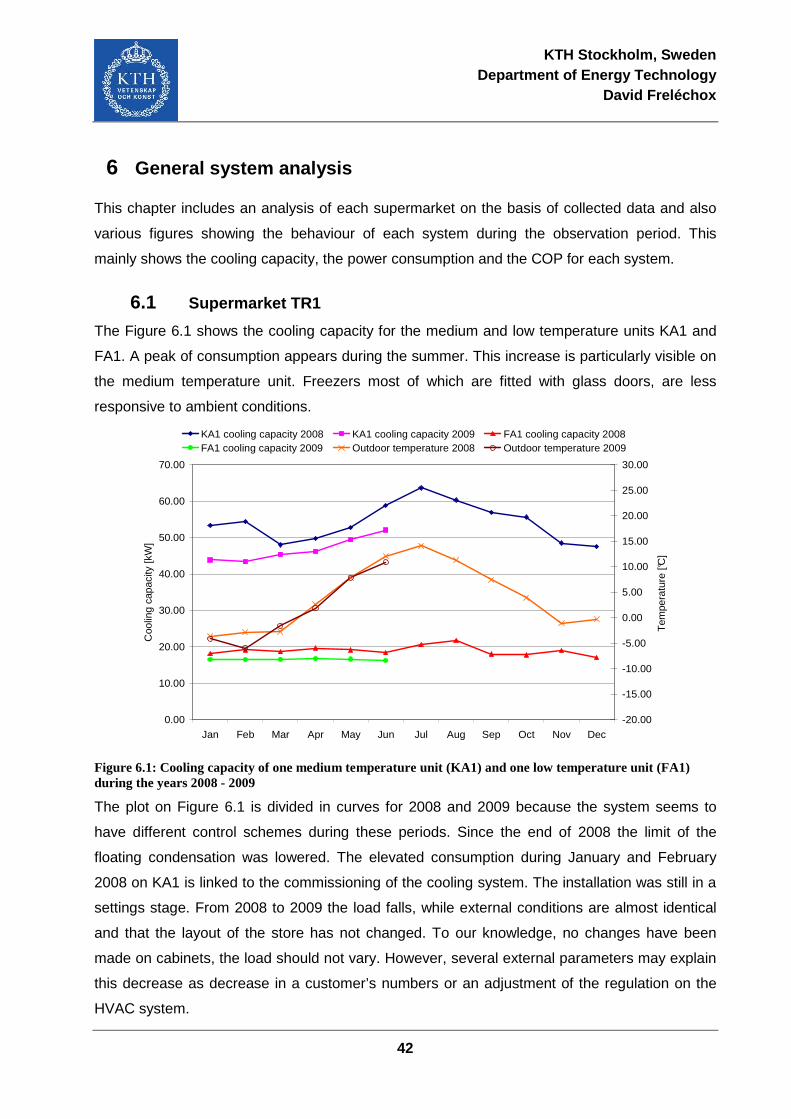
KTH Stockholm, Sweden Department of Energy Technology
David Freléchox
42
6 General system analysis
This chapter includes an analysis of each supermarket on the basis of collected data and also
various figures showing the behaviour of each system during the observation period. This
mainly shows the cooling capacity, the power consumption and the COP for each system.
6.1 Supermarket TR1
The Figure 6.1 shows the cooling capacity for the medium and low temperature units KA1 and
FA1. A peak of consumption appears during the summer. This increase is particularly visible on
the medium temperature unit. Freezers most of which are fitted with glass doors, are less
responsive to ambient conditions.
0.00
10.00
20.00
30.00
40.00
50.00
60.00
70.00
Jan Feb Mar Apr May Jun Jul Aug Sep Oct Nov Dec
Coo
ling
capa
city
[kW
]
-20.00
-15.00
-10.00
-5.00
0.00
5.00
10.00
15.00
20.00
25.00
30.00
Tem
pera
ture
[°C
]
KA1 cooling capacity 2008 KA1 cooling capacity 2009 FA1 cooling capacity 2008FA1 cooling capacity 2009 Outdoor temperature 2008 Outdoor temperature 2009
Figure 6.1: Cooling capacity of one medium temperature unit (KA1) and one low temperature unit (FA1) during the years 2008 - 2009
The plot on Figure 6.1 is divided in curves for 2008 and 2009 because the system seems to
have different control schemes during these periods. Since the end of 2008 the limit of the
floating condensation was lowered. The elevated consumption during January and February
2008 on KA1 is linked to the commissioning of the cooling system. The installation was still in a
settings stage. From 2008 to 2009 the load falls, while external conditions are almost identical
and that the layout of the store has not changed. To our knowledge, no changes have been
made on cabinets, the load should not vary. However, several external parameters may explain
this decrease as decrease in a customer’s numbers or an adjustment of the regulation on the
HVAC system.
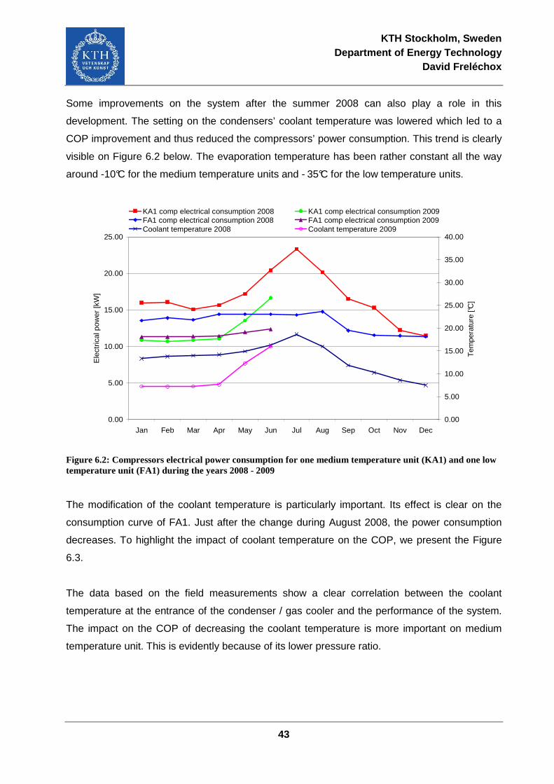
KTH Stockholm, Sweden Department of Energy Technology
David Freléchox
43
Some improvements on the system after the summer 2008 can also play a role in this
development. The setting on the condensers’ coolant temperature was lowered which led to a
COP improvement and thus reduced the compressors’ power consumption. This trend is clearly
visible on Figure 6.2 below. The evaporation temperature has been rather constant all the way
around -10°C for the medium temperature units and - 35°C for the low temperature units.
0.00
5.00
10.00
15.00
20.00
25.00
Jan Feb Mar Apr May Jun Jul Aug Sep Oct Nov Dec
Ele
ctric
al p
ower
[kW
]
0.00
5.00
10.00
15.00
20.00
25.00
30.00
35.00
40.00
Tem
pera
ture
[°C
]
KA1 comp electrical consumption 2008 KA1 comp electrical consumption 2009FA1 comp electrical consumption 2008 FA1 comp electrical consumption 2009Coolant temperature 2008 Coolant temperature 2009
Figure 6.2: Compressors electrical power consumption for one medium temperature unit (KA1) and one low temperature unit (FA1) during the years 2008 - 2009
The modification of the coolant temperature is particularly important. Its effect is clear on the
consumption curve of FA1. Just after the change during August 2008, the power consumption
decreases. To highlight the impact of coolant temperature on the COP, we present the Figure
6.3.
The data based on the field measurements show a clear correlation between the coolant
temperature at the entrance of the condenser / gas cooler and the performance of the system.
The impact on the COP of decreasing the coolant temperature is more important on medium
temperature unit. This is evidently because of its lower pressure ratio.
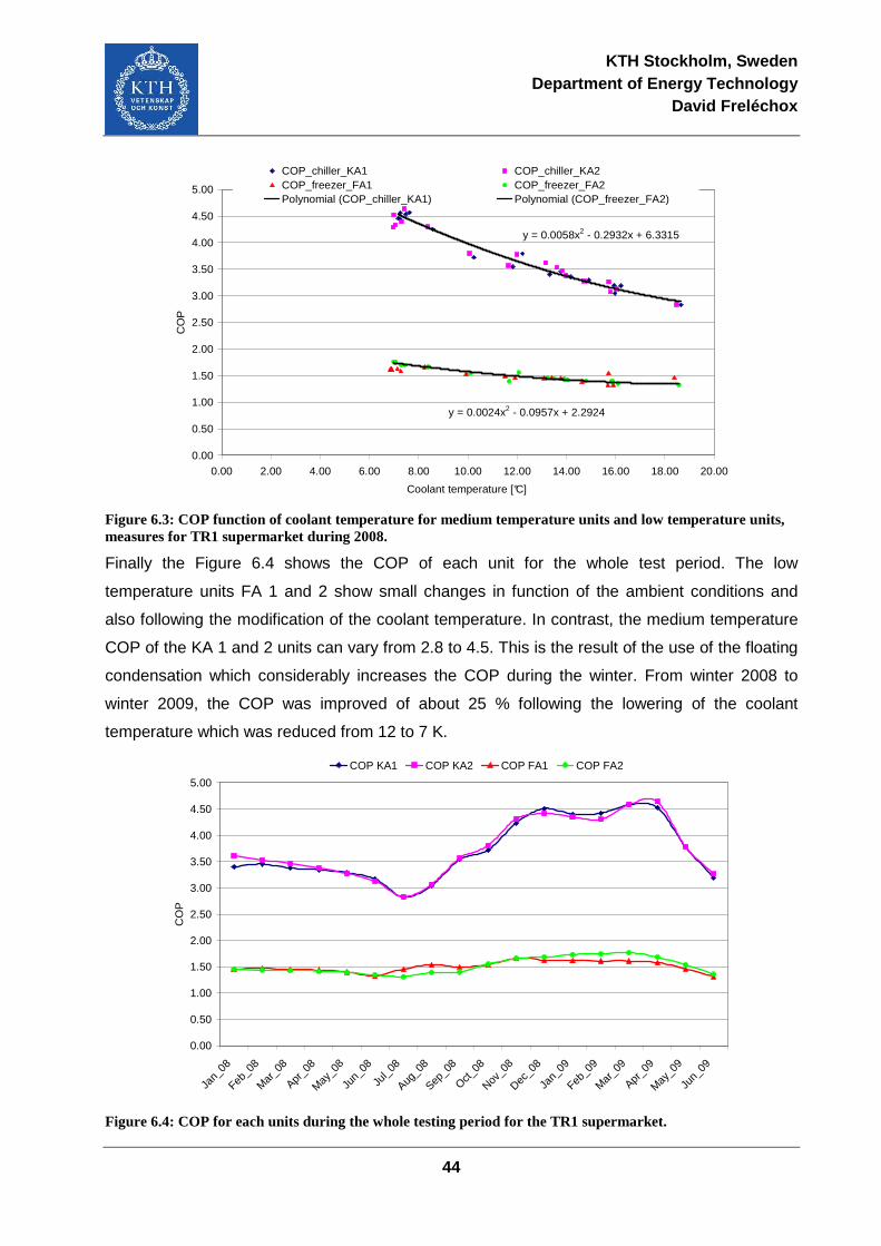
KTH Stockholm, Sweden Department of Energy Technology
David Freléchox
44
y = 0.0058x2 - 0.2932x + 6.3315
y = 0.0024x2 - 0.0957x + 2.2924
0.00
0.50
1.00
1.50
2.00
2.50
3.00
3.50
4.00
4.50
5.00
0.00 2.00 4.00 6.00 8.00 10.00 12.00 14.00 16.00 18.00 20.00
Coolant temperature [°C]
CO
PCOP_chiller_KA1 COP_chiller_KA2COP_freezer_FA1 COP_freezer_FA2Polynomial (COP_chiller_KA1) Polynomial (COP_freezer_FA2)
Figure 6.3: COP function of coolant temperature for medium temperature units and low temperature units, measures for TR1 supermarket during 2008.
Finally the Figure 6.4 shows the COP of each unit for the whole test period. The low
temperature units FA 1 and 2 show small changes in function of the ambient conditions and
also following the modification of the coolant temperature. In contrast, the medium temperature
COP of the KA 1 and 2 units can vary from 2.8 to 4.5. This is the result of the use of the floating
condensation which considerably increases the COP during the winter. From winter 2008 to
winter 2009, the COP was improved of about 25 % following the lowering of the coolant
temperature which was reduced from 12 to 7 K.
0.00
0.50
1.00
1.50
2.00
2.50
3.00
3.50
4.00
4.50
5.00
Jan_
08
Feb_0
8
Mar
_08
Apr_0
8
May
_08
Jun_
08
Jul_0
8
Aug_0
8
Sep_0
8
Oct_08
Nov_0
8
Dec_0
8
Jan_
09
Feb_0
9
Mar
_09
Apr_0
9
May
_09
Jun_
09
CO
P
COP KA1 COP KA2 COP FA1 COP FA2
Figure 6.4: COP for each units during the whole testing period for the TR1 supermarket.

KTH Stockholm, Sweden Department of Energy Technology
David Freléchox
45
6.2 Supermarket TR2
A figure per unit has been achieved, KAFA 1 and 2 are booster units and KA3 is a medium
temperature unit. These figures show the evolution of the cooling power and the related power
consumption, the curves of condensing and outdoor temperature, as well as the effect of
subcooling produced by the borehole. This effect is expressed by its ∆T in Kelvin. Note that the
borehole is connected to the heat pump as well and used as heat source to heat the building
during the winter.
0.00
10.00
20.00
30.00
40.00
50.00
60.00
70.00
Sept_
08
Oct_08
Nov_0
8
Dec_0
8
Jan_
09
Feb_
09
Mar
ch_0
9
April_
09
May
_09
June
_09
Coo
ling
capa
city
[kW
] - E
lect
rical
pow
er [k
W]
0.00
5.00
10.00
15.00
20.00
25.00
30.00
Tem
pera
ture
[°C
] - d
T [K
]
Cooling capacity Compressor electrical consumptionCondensation temperature dT subcooling boreholeOutside temperature
Tevap = -10°C / -35°C
Figure 6.5: Different parameters plots for the KAFA1 unit during the whole period of study in the TR2 supermarket
Figure 6.5 shows, as expected a cooling capacity drop during the winter. In contrast the power
consumption does not follow the same trend, although logically it should take advantage of low
winter temperatures. The cause is simply forcing the condensing temperature at about 25°C in
order to increase the capacity for the heat recovery system. The refrigeration system and heat
pump are connected via the borehole but also on the "warm" side through a plate heat
exchanger disposed on the high pressure circuit at the compressor exit.
To compensate this rise of the condensation temperature and in order to maintain the COP at a
high level, the borehole is used to subcool the fluid. Note that the higher the condensing
temperature is kept, the greater is the ∆T subcooling. The fact that the heat pump for heating
the store is also connected to the borehole can justify this principle of operation as the rejected
heat by the subcooling can then be used by the heat pump. Similar parameters plots as in the
previous figure have been developed for KAFA2 in Figure 6.6 and for KA3 in Figure 6.7.
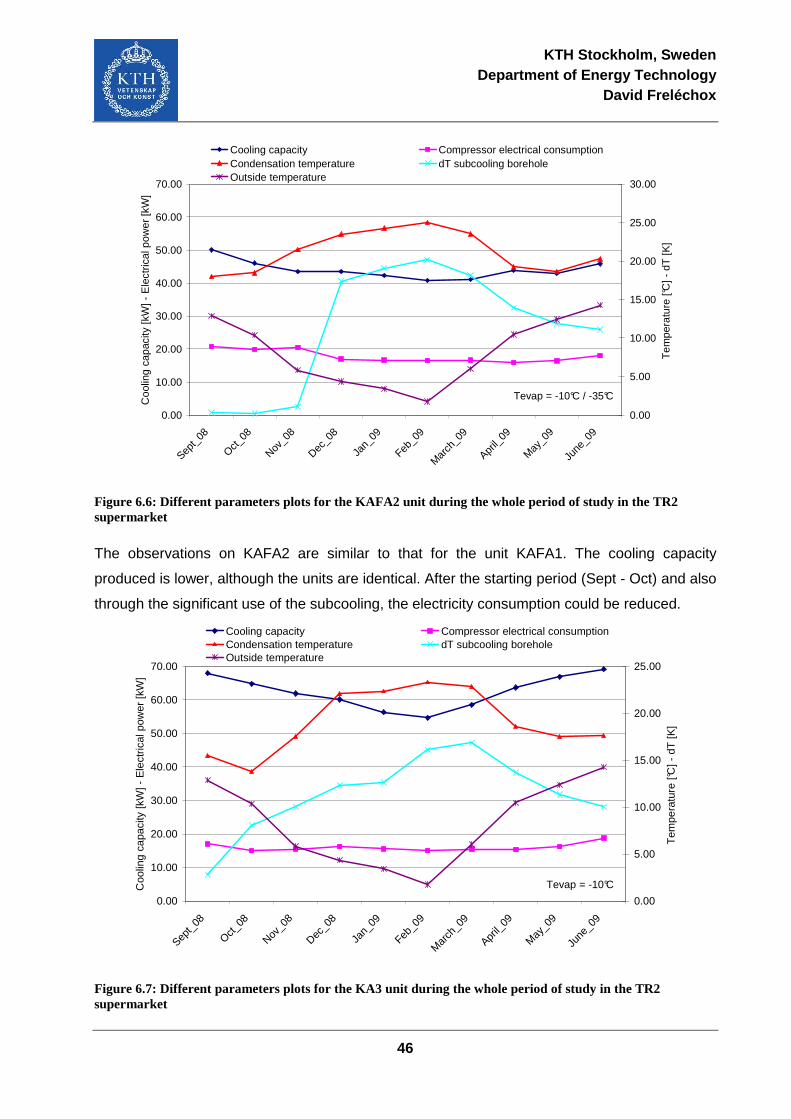
KTH Stockholm, Sweden Department of Energy Technology
David Freléchox
46
0.00
10.00
20.00
30.00
40.00
50.00
60.00
70.00
Sept_
08
Oct_08
Nov_0
8
Dec_0
8
Jan_
09
Feb_0
9
Mar
ch_0
9
April_
09
May_0
9
June
_09
Coo
ling
capa
city
[kW
] - E
lect
rical
pow
er [k
W]
0.00
5.00
10.00
15.00
20.00
25.00
30.00
Tem
pera
ture
[°C
] - d
T [K
]
Cooling capacity Compressor electrical consumptionCondensation temperature dT subcooling boreholeOutside temperature
Tevap = -10°C / -35°C
Figure 6.6: Different parameters plots for the KAFA2 unit during the whole period of study in the TR2 supermarket
The observations on KAFA2 are similar to that for the unit KAFA1. The cooling capacity
produced is lower, although the units are identical. After the starting period (Sept - Oct) and also
through the significant use of the subcooling, the electricity consumption could be reduced.
0.00
10.00
20.00
30.00
40.00
50.00
60.00
70.00
Sept_
08
Oct_08
Nov_0
8
Dec_0
8
Jan_
09
Feb_0
9
Mar
ch_0
9
April_
09
May
_09
June
_09
Coo
ling
capa
city
[kW
] - E
lect
rical
pow
er [k
W]
0.00
5.00
10.00
15.00
20.00
25.00T
empe
ratu
re [°
C] -
dT
[K]
Cooling capacity Compressor electrical consumptionCondensation temperature dT subcooling boreholeOutside temperature
Tevap = -10°C
Figure 6.7: Different parameters plots for the KA3 unit during the whole period of study in the TR2 supermarket
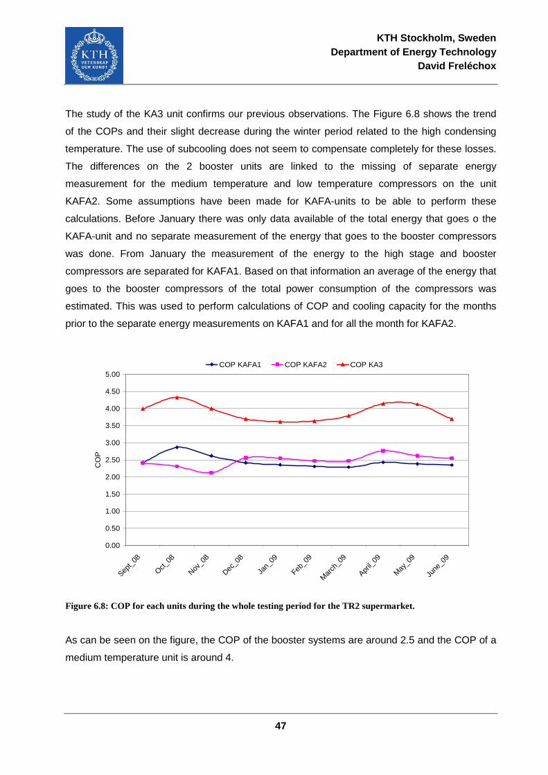
KTH Stockholm, Sweden Department of Energy Technology
David Freléchox
47
The study of the KA3 unit confirms our previous observations. The Figure 6.8 shows the trend
of the COPs and their slight decrease during the winter period related to the high condensing
temperature. The use of subcooling does not seem to compensate completely for these losses.
The differences on the 2 booster units are linked to the missing of separate energy
measurement for the medium temperature and low temperature compressors on the unit
KAFA2. Some assumptions have been made for KAFA-units to be able to perform these
calculations. Before January there was only data available of the total energy that goes o the
KAFA-unit and no separate measurement of the energy that goes to the booster compressors
was done. From January the measurement of the energy to the high stage and booster
compressors are separated for KAFA1. Based on that information an average of the energy that
goes to the booster compressors of the total power consumption of the compressors was
estimated. This was used to perform calculations of COP and cooling capacity for the months
prior to the separate energy measurements on KAFA1 and for all the month for KAFA2.
0.00
0.50
1.00
1.50
2.00
2.50
3.00
3.50
4.00
4.50
5.00
Sept_
08
Oct_08
Nov_0
8
Dec_0
8
Jan_
09
Feb_0
9
Mar
ch_0
9
April_
09
May
_09
June
_09
CO
P
COP KAFA1 COP KAFA2 COP KA3
Figure 6.8: COP for each units during the whole testing period for the TR2 supermarket.
As can be seen on the figure, the COP of the booster systems are around 2.5 and the COP of a
medium temperature unit is around 4.
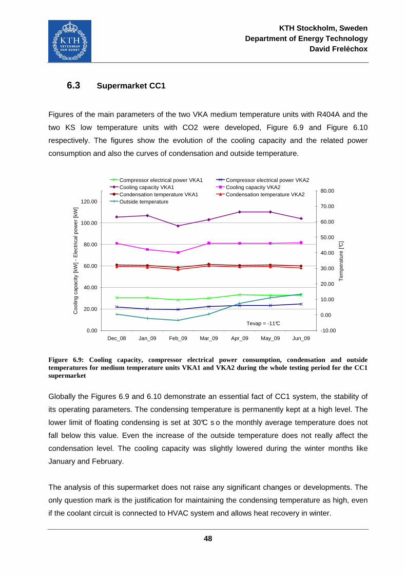
KTH Stockholm, Sweden Department of Energy Technology
David Freléchox
48
6.3 Supermarket CC1
Figures of the main parameters of the two VKA medium temperature units with R404A and the
two KS low temperature units with CO2 were developed, Figure 6.9 and Figure 6.10
respectively. The figures show the evolution of the cooling capacity and the related power
consumption and also the curves of condensation and outside temperature.
0.00
20.00
40.00
60.00
80.00
100.00
120.00
Dec_08 Jan_09 Feb_09 Mar_09 Apr_09 May_09 Jun_09
Coo
ling
capa
city
[kW
] - E
lect
rical
pow
er [k
W]
-10.00
0.00
10.00
20.00
30.00
40.00
50.00
60.00
70.00
80.00
Tem
pera
ture
[°C
]
Compressor electrical power VKA1 Compressor electrical power VKA2Cooling capacity VKA1 Cooling capacity VKA2Condensation temperature VKA1 Condensation temperature VKA2Outside temperature
Tevap = -11°C
Figure 6.9: Cooling capacity, compressor electrical power consumption, condensation and outside temperatures for medium temperature units VKA1 and VKA2 during the whole testing period for the CC1 supermarket
Globally the Figures 6.9 and 6.10 demonstrate an essential fact of CC1 system, the stability of
its operating parameters. The condensing temperature is permanently kept at a high level. The
lower limit of floating condensing is set at 30°C s o the monthly average temperature does not
fall below this value. Even the increase of the outside temperature does not really affect the
condensation level. The cooling capacity was slightly lowered during the winter months like
January and February.
The analysis of this supermarket does not raise any significant changes or developments. The
only question mark is the justification for maintaining the condensing temperature as high, even
if the coolant circuit is connected to HVAC system and allows heat recovery in winter.
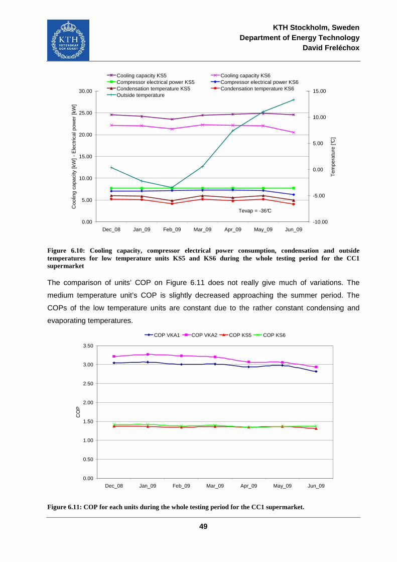
KTH Stockholm, Sweden Department of Energy Technology
David Freléchox
49
0.00
5.00
10.00
15.00
20.00
25.00
30.00
Dec_08 Jan_09 Feb_09 Mar_09 Apr_09 May_09 Jun_09
Coo
ling
capa
city
[kW
] - E
lect
rical
pow
er [k
W]
-10.00
-5.00
0.00
5.00
10.00
15.00
Tem
pera
ture
[°C
]
Cooling capacity KS5 Cooling capacity KS6Compressor electrical power KS5 Compressor electrical power KS6Condensation temperature KS5 Condensation temperature KS6Outside temperature
Tevap = -36°C
Figure 6.10: Cooling capacity, compressor electrical power consumption, condensation and outside temperatures for low temperature units KS5 and KS6 during the whole testing period for the CC1 supermarket
The comparison of units’ COP on Figure 6.11 does not really give much of variations. The
medium temperature unit’s COP is slightly decreased approaching the summer period. The
COPs of the low temperature units are constant due to the rather constant condensing and
evaporating temperatures.
0.00
0.50
1.00
1.50
2.00
2.50
3.00
3.50
Dec_08 Jan_09 Feb_09 Mar_09 Apr_09 May_09 Jun_09
CO
P
COP VKA1 COP VKA2 COP KS5 COP KS6
Figure 6.11: COP for each units during the whole testing period for the CC1 supermarket.
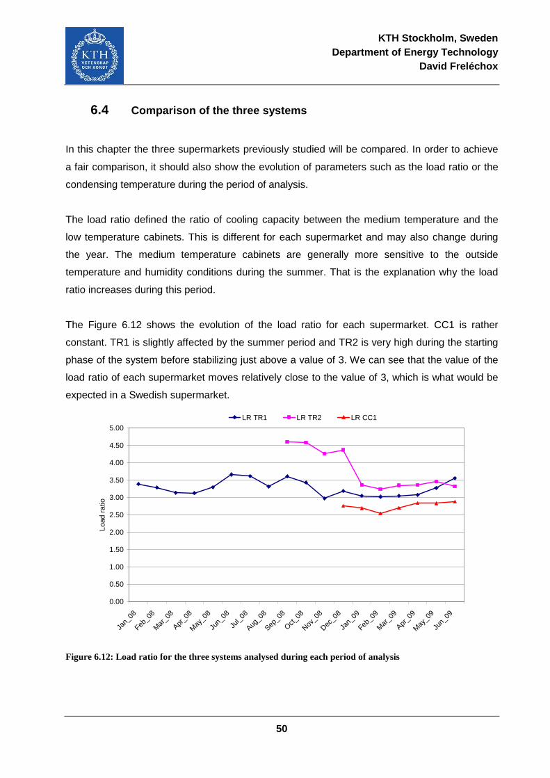
KTH Stockholm, Sweden Department of Energy Technology
David Freléchox
50
6.4 Comparison of the three systems
In this chapter the three supermarkets previously studied will be compared. In order to achieve
a fair comparison, it should also show the evolution of parameters such as the load ratio or the
condensing temperature during the period of analysis.
The load ratio defined the ratio of cooling capacity between the medium temperature and the
low temperature cabinets. This is different for each supermarket and may also change during
the year. The medium temperature cabinets are generally more sensitive to the outside
temperature and humidity conditions during the summer. That is the explanation why the load
ratio increases during this period.
The Figure 6.12 shows the evolution of the load ratio for each supermarket. CC1 is rather
constant. TR1 is slightly affected by the summer period and TR2 is very high during the starting
phase of the system before stabilizing just above a value of 3. We can see that the value of the
load ratio of each supermarket moves relatively close to the value of 3, which is what would be
expected in a Swedish supermarket.
0.00
0.50
1.00
1.50
2.00
2.50
3.00
3.50
4.00
4.50
5.00
Jan_
08
Feb_0
8
Mar
_08
Apr_0
8
May
_08
Jun_
08
Jul_0
8
Aug_0
8
Sep_0
8
Oct_08
Nov_0
8
Dec_0
8
Jan_
09
Feb_0
9
Mar
_09
Apr_0
9
May
_09
Jun_
09
Load
rat
io
LR TR1 LR TR2 LR CC1
Figure 6.12: Load ratio for the three systems analysed during each period of analysis
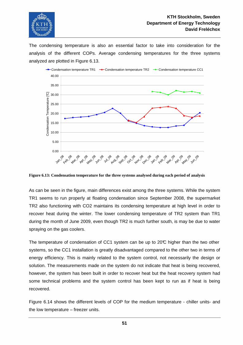
KTH Stockholm, Sweden Department of Energy Technology
David Freléchox
51
The condensing temperature is also an essential factor to take into consideration for the
analysis of the different COPs. Average condensing temperatures for the three systems
analyzed are plotted in Figure 6.13.
0.00
5.00
10.00
15.00
20.00
25.00
30.00
35.00
40.00
Jan_
08
Feb_0
8
Mar
_08
Apr_0
8
May_0
8
Jun_
08
Jul_0
8
Aug_0
8
Sep_0
8
Oct_08
Nov_0
8
Dec_0
8
Jan_
09
Feb_0
9
Mar
_09
Apr_0
9
May_0
9
Jun_
09
Con
dens
atio
n T
empe
ratu
re [°
C]
Condensation temperature TR1 Condensation temperature TR2 Condensation temperature CC1
Figure 6.13: Condensation temperature for the three systems analysed during each period of analysis
As can be seen in the figure, main differences exist among the three systems. While the system
TR1 seems to run properly at floating condensation since September 2008, the supermarket
TR2 also functioning with CO2 maintains its condensing temperature at high level in order to
recover heat during the winter. The lower condensing temperature of TR2 system than TR1
during the month of June 2009, even though TR2 is much further south, is may be due to water
spraying on the gas coolers.
The temperature of condensation of CC1 system can be up to 20°C higher than the two other
systems, so the CC1 installation is greatly disadvantaged compared to the other two in terms of
energy efficiency. This is mainly related to the system control, not necessarily the design or
solution. The measurements made on the system do not indicate that heat is being recovered,
however, the system has been built in order to recover heat but the heat recovery system had
some technical problems and the system control has been kept to run as if heat is being
recovered.
Figure 6.14 shows the different levels of COP for the medium temperature - chiller units- and
the low temperature – freezer units.
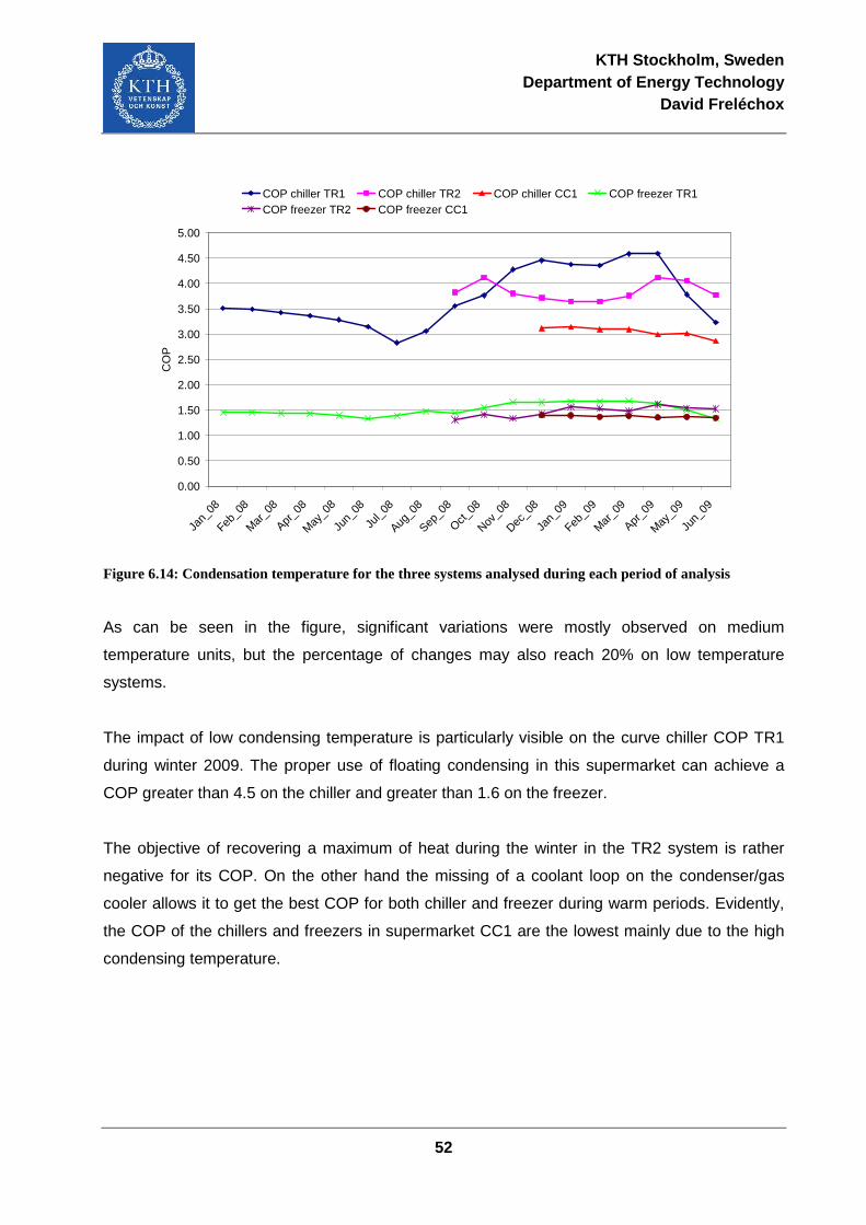
KTH Stockholm, Sweden Department of Energy Technology
David Freléchox
52
0.00
0.50
1.00
1.50
2.00
2.50
3.00
3.50
4.00
4.50
5.00
Jan_
08
Feb_0
8
Mar
_08
Apr_0
8
May
_08
Jun_
08
Jul_0
8
Aug_0
8
Sep_0
8
Oct_08
Nov_0
8
Dec_0
8
Jan_
09
Feb_0
9
Mar
_09
Apr_0
9
May
_09
Jun_
09
CO
P
COP chiller TR1 COP chiller TR2 COP chiller CC1 COP freezer TR1COP freezer TR2 COP freezer CC1
Figure 6.14: Condensation temperature for the three systems analysed during each period of analysis
As can be seen in the figure, significant variations were mostly observed on medium
temperature units, but the percentage of changes may also reach 20% on low temperature
systems.
The impact of low condensing temperature is particularly visible on the curve chiller COP TR1
during winter 2009. The proper use of floating condensing in this supermarket can achieve a
COP greater than 4.5 on the chiller and greater than 1.6 on the freezer.
The objective of recovering a maximum of heat during the winter in the TR2 system is rather
negative for its COP. On the other hand the missing of a coolant loop on the condenser/gas
cooler allows it to get the best COP for both chiller and freezer during warm periods. Evidently,
the COP of the chillers and freezers in supermarket CC1 are the lowest mainly due to the high
condensing temperature.
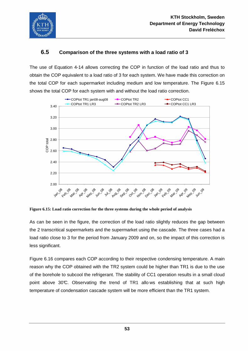
KTH Stockholm, Sweden Department of Energy Technology
David Freléchox
53
6.5 Comparison of the three systems with a load ratio o f 3
The use of Equation 4-14 allows correcting the COP in function of the load ratio and thus to
obtain the COP equivalent to a load ratio of 3 for each system. We have made this correction on
the total COP for each supermarket including medium and low temperature. The Figure 6.15
shows the total COP for each system with and without the load ratio correction.
2.00
2.20
2.40
2.60
2.80
3.00
3.20
3.40
Jan_
08
Feb_0
8
Mar
_08
Apr_0
8
May
_08
Jun_
08
Jul_0
8
Aug_0
8
Sep_0
8
Oct_08
Nov_0
8
Dec_0
8
Jan_
09
Feb_0
9
Mar
_09
Apr_0
9
May
_09
Jun_
09
CO
P to
tal
COPtot TR1 jan08-aug08 COPtot TR2 COPtot CC1 COPtot TR1 LR3 COPtot TR2 LR3 COPtot CC1 LR3
Figure 6.15: Load ratio correction for the three systems during the whole period of analysis
As can be seen in the figure, the correction of the load ratio slightly reduces the gap between
the 2 transcritical supermarkets and the supermarket using the cascade. The three cases had a
load ratio close to 3 for the period from January 2009 and on, so the impact of this correction is
less significant.
Figure 6.16 compares each COP according to their respective condensing temperature. A main
reason why the COP obtained with the TR2 system could be higher than TR1 is due to the use
of the borehole to subcool the refrigerant. The stability of CC1 operation results in a small cloud
point above 30°C. Observating the trend of TR1 allo ws establishing that at such high
temperature of condensation cascade system will be more efficient than the TR1 system.
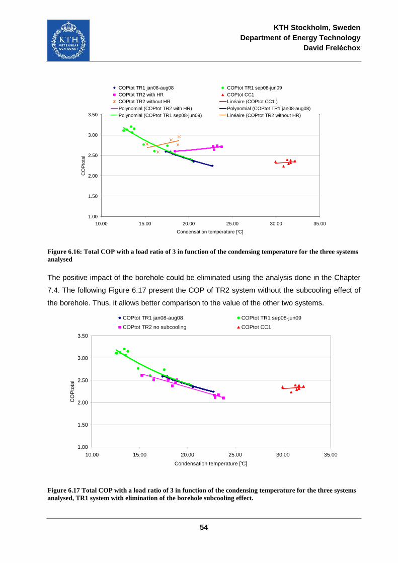
KTH Stockholm, Sweden Department of Energy Technology
David Freléchox
54
1.00
1.50
2.00
2.50
3.00
3.50
10.00 15.00 20.00 25.00 30.00 35.00
Condensation temperature [°C]
CO
Pto
tal
COPtot TR1 jan08-aug08 COPtot TR1 sep08-jun09COPtot TR2 with HR COPtot CC1 COPtot TR2 without HR Linéaire (COPtot CC1 )Polynomial (COPtot TR2 with HR) Polynomial (COPtot TR1 jan08-aug08)Polynomial (COPtot TR1 sep08-jun09) Linéaire (COPtot TR2 without HR)
Figure 6.16: Total COP with a load ratio of 3 in function of the condensing temperature for the three systems analysed
The positive impact of the borehole could be eliminated using the analysis done in the Chapter
7.4. The following Figure 6.17 present the COP of TR2 system without the subcooling effect of
the borehole. Thus, it allows better comparison to the value of the other two systems.
1.00
1.50
2.00
2.50
3.00
3.50
10.00 15.00 20.00 25.00 30.00 35.00
Condensation temperature [°C]
CO
Pto
tal
COPtot TR1 jan08-aug08 COPtot TR1 sep08-jun09
COPtot TR2 no subcooling COPtot CC1
Figure 6.17 Total COP with a load ratio of 3 in function of the condensing temperature for the three systems analysed, TR1 system with elimination of the borehole subcooling effect.
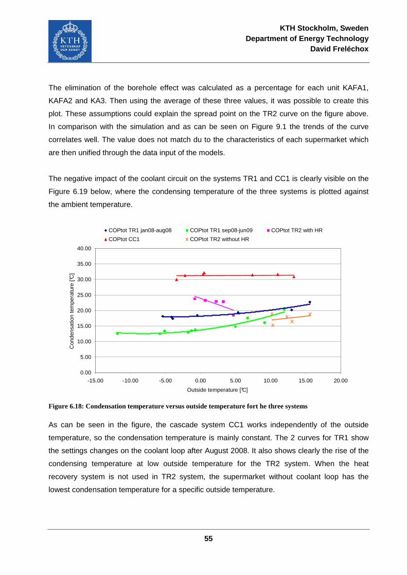
KTH Stockholm, Sweden Department of Energy Technology
David Freléchox
55
The elimination of the borehole effect was calculated as a percentage for each unit KAFA1,
KAFA2 and KA3. Then using the average of these three values, it was possible to create this
plot. These assumptions could explain the spread point on the TR2 curve on the figure above.
In comparison with the simulation and as can be seen on Figure 9.1 the trends of the curve
correlates well. The value does not match du to the characteristics of each supermarket which
are then unified through the data input of the models.
The negative impact of the coolant circuit on the systems TR1 and CC1 is clearly visible on the
Figure 6.19 below, where the condensing temperature of the three systems is plotted against
the ambient temperature.
0.00
5.00
10.00
15.00
20.00
25.00
30.00
35.00
40.00
-15.00 -10.00 -5.00 0.00 5.00 10.00 15.00 20.00
Outside temperature [°C]
Con
dens
atio
n te
mpe
ratu
re [°
C]
COPtot TR1 jan08-aug08 COPtot TR1 sep08-jun09 COPtot TR2 with HR
COPtot CC1 COPtot TR2 without HR
Figure 6.18: Condensation temperature versus outside temperature fort he three systems
As can be seen in the figure, the cascade system CC1 works independently of the outside
temperature, so the condensation temperature is mainly constant. The 2 curves for TR1 show
the settings changes on the coolant loop after August 2008. It also shows clearly the rise of the
condensing temperature at low outside temperature for the TR2 system. When the heat
recovery system is not used in TR2 system, the supermarket without coolant loop has the
lowest condensation temperature for a specific outside temperature.
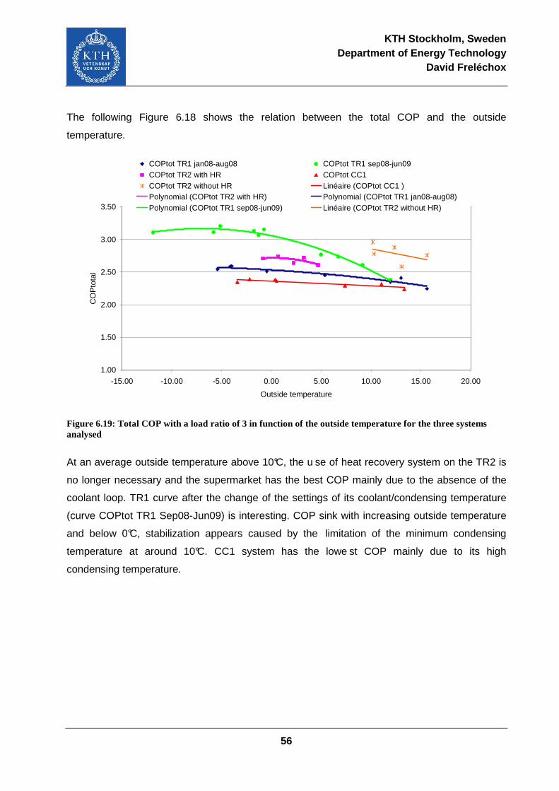
KTH Stockholm, Sweden Department of Energy Technology
David Freléchox
56
The following Figure 6.18 shows the relation between the total COP and the outside
temperature.
1.00
1.50
2.00
2.50
3.00
3.50
-15.00 -10.00 -5.00 0.00 5.00 10.00 15.00 20.00
Outside temperature
CO
Pto
tal
COPtot TR1 jan08-aug08 COPtot TR1 sep08-jun09COPtot TR2 with HR COPtot CC1 COPtot TR2 without HR Linéaire (COPtot CC1 )Polynomial (COPtot TR2 with HR) Polynomial (COPtot TR1 jan08-aug08)Polynomial (COPtot TR1 sep08-jun09) Linéaire (COPtot TR2 without HR)
Figure 6.19: Total COP with a load ratio of 3 in function of the outside temperature for the three systems analysed
At an average outside temperature above 10°C, the u se of heat recovery system on the TR2 is
no longer necessary and the supermarket has the best COP mainly due to the absence of the
coolant loop. TR1 curve after the change of the settings of its coolant/condensing temperature
(curve COPtot TR1 Sep08-Jun09) is interesting. COP sink with increasing outside temperature
and below 0°C, stabilization appears caused by the limitation of the minimum condensing
temperature at around 10°C. CC1 system has the lowe st COP mainly due to its high
condensing temperature.
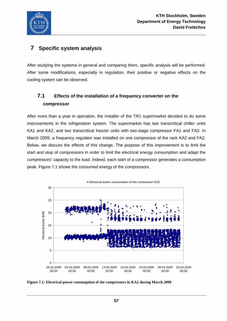
KTH Stockholm, Sweden Department of Energy Technology
David Freléchox
57
7 Specific system analysis
After studying the systems in general and comparing them, specific analysis will be performed.
After some modifications, especially in regulation, their positive or negative effects on the
cooling system can be observed.
7.1 Effects of the installation of a frequency converte r on the
compressor
After more than a year in operation, the installer of the TR1 supermarket decided to do some
improvements in the refrigeration system. The supermarket has two transcritical chiller units
KA1 and KA2, and two transcritical freezer units with two-stage compressor FA1 and FA2. In
March 2009, a frequency regulator was installed on one compressor of the rack KA2 and FA2.
Below, we discuss the effects of this change. The purpose of this improvement is to limit the
start and stop of compressors in order to limit the electrical energy consumption and adapt the
compressors’ capacity to the load. Indeed, each start of a compressor generates a consumption
peak. Figure 7.1 shows the consumed energy of the compressors.
0
5
10
15
20
25
30
26.02.200900:00
03.03.200900:00
08.03.200900:00
13.03.200900:00
18.03.200900:00
23.03.200900:00
28.03.200900:00
02.04.200900:00
Ele
ctric
al p
ower
[kW
]
Electrical power consumption of the compressor KA2
Figure 7.1: Electrical power consumption of the compressors in KA2 during March 2009
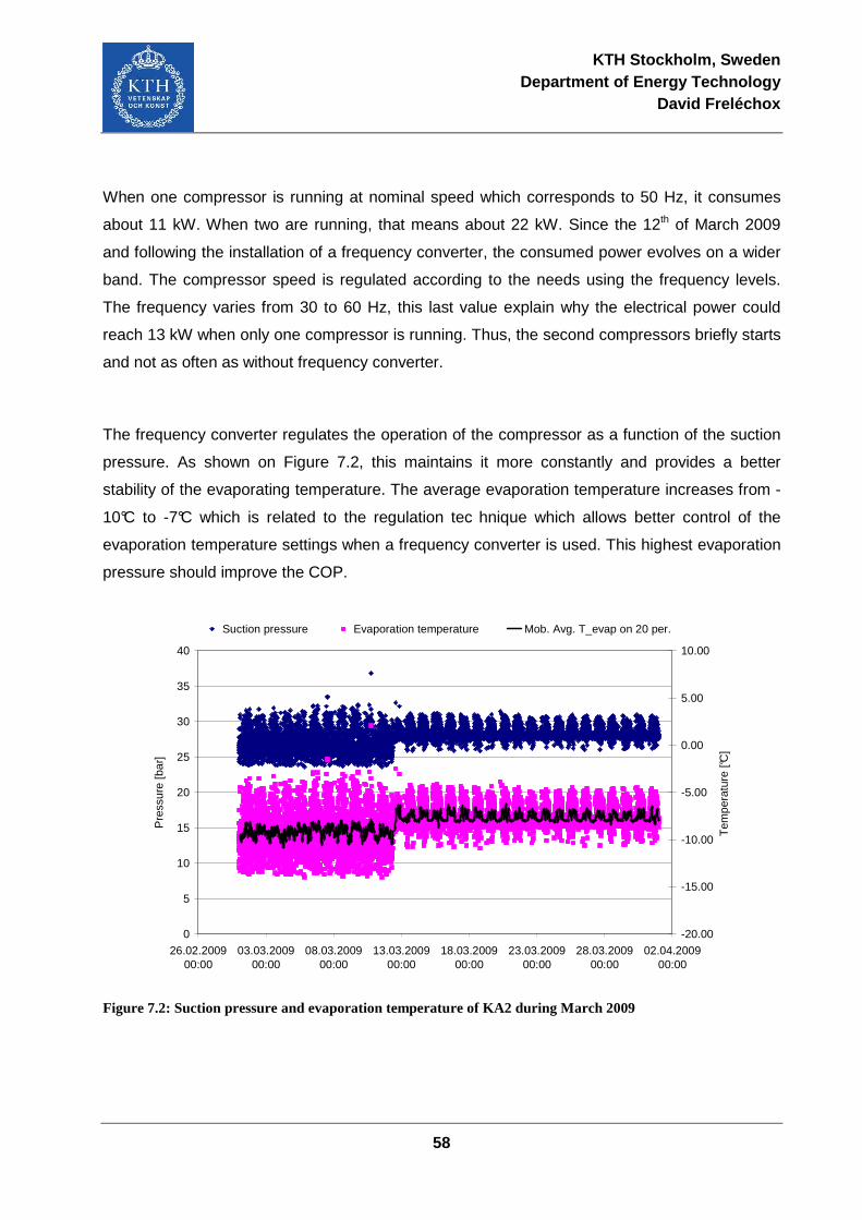
KTH Stockholm, Sweden Department of Energy Technology
David Freléchox
58
When one compressor is running at nominal speed which corresponds to 50 Hz, it consumes
about 11 kW. When two are running, that means about 22 kW. Since the 12th of March 2009
and following the installation of a frequency converter, the consumed power evolves on a wider
band. The compressor speed is regulated according to the needs using the frequency levels.
The frequency varies from 30 to 60 Hz, this last value explain why the electrical power could
reach 13 kW when only one compressor is running. Thus, the second compressors briefly starts
and not as often as without frequency converter.
The frequency converter regulates the operation of the compressor as a function of the suction
pressure. As shown on Figure 7.2, this maintains it more constantly and provides a better
stability of the evaporating temperature. The average evaporation temperature increases from -
10°C to -7°C which is related to the regulation tec hnique which allows better control of the
evaporation temperature settings when a frequency converter is used. This highest evaporation
pressure should improve the COP.
0
5
10
15
20
25
30
35
40
26.02.200900:00
03.03.200900:00
08.03.200900:00
13.03.200900:00
18.03.200900:00
23.03.200900:00
28.03.200900:00
02.04.200900:00
Pre
ssur
e [b
ar]
-20.00
-15.00
-10.00
-5.00
0.00
5.00
10.00
Tem
pera
ture
[°C
]
Suction pressure Evaporation temperature Mob. Avg. T_evap on 20 per.
Figure 7.2: Suction pressure and evaporation temperature of KA2 during March 2009
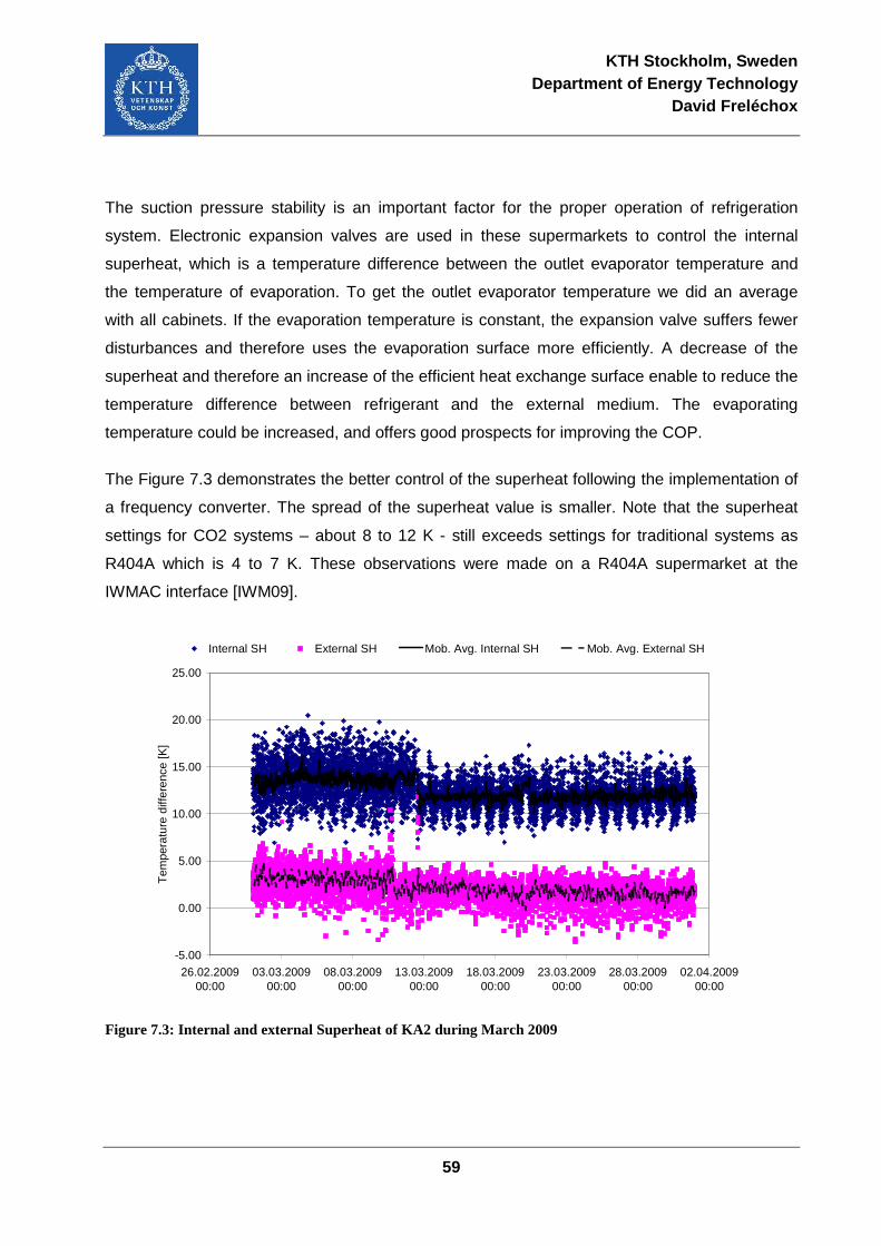
KTH Stockholm, Sweden Department of Energy Technology
David Freléchox
59
The suction pressure stability is an important factor for the proper operation of refrigeration
system. Electronic expansion valves are used in these supermarkets to control the internal
superheat, which is a temperature difference between the outlet evaporator temperature and
the temperature of evaporation. To get the outlet evaporator temperature we did an average
with all cabinets. If the evaporation temperature is constant, the expansion valve suffers fewer
disturbances and therefore uses the evaporation surface more efficiently. A decrease of the
superheat and therefore an increase of the efficient heat exchange surface enable to reduce the
temperature difference between refrigerant and the external medium. The evaporating
temperature could be increased, and offers good prospects for improving the COP.
The Figure 7.3 demonstrates the better control of the superheat following the implementation of
a frequency converter. The spread of the superheat value is smaller. Note that the superheat
settings for CO2 systems – about 8 to 12 K - still exceeds settings for traditional systems as
R404A which is 4 to 7 K. These observations were made on a R404A supermarket at the
IWMAC interface [IWM09].
-5.00
0.00
5.00
10.00
15.00
20.00
25.00
26.02.200900:00
03.03.200900:00
08.03.200900:00
13.03.200900:00
18.03.200900:00
23.03.200900:00
28.03.200900:00
02.04.200900:00
Tem
pera
ture
diff
eren
ce [K
]
Internal SH External SH Mob. Avg. Internal SH Mob. Avg. External SH
Figure 7.3: Internal and external Superheat of KA2 during March 2009
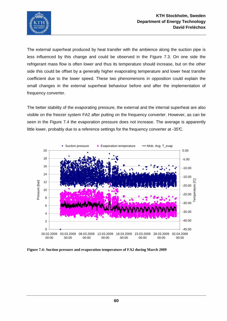
KTH Stockholm, Sweden Department of Energy Technology
David Freléchox
60
The external superheat produced by heat transfer with the ambience along the suction pipe is
less influenced by this change and could be observed in the Figure 7.3. On one side the
refrigerant mass flow is often lower and thus its temperature should increase, but on the other
side this could be offset by a generally higher evaporating temperature and lower heat transfer
coefficient due to the lower speed. These two phenomenons in opposition could explain the
small changes in the external superheat behaviour before and after the implementation of
frequency converter.
The better stability of the evaporating pressure, the external and the internal superheat are also
visible on the freezer system FA2 after putting on the frequency converter. However, as can be
seen in the Figure 7.4 the evaporation pressure does not increase. The average is apparently
little lower, probably due to a reference settings for the frequency converter at -35°C.
0
2
4
6
8
10
12
14
16
18
20
26.02.200900:00
03.03.200900:00
08.03.200900:00
13.03.200900:00
18.03.200900:00
23.03.200900:00
28.03.200900:00
02.04.200900:00
Pre
ssur
e [b
ar]
-45.00
-40.00
-35.00
-30.00
-25.00
-20.00
-15.00
-10.00
-5.00
0.00
Tem
pera
ture
[°C
]
Suction pressure Evaporation temperature Mob. Avg. T_evap
Figure 7.4: Suction pressure and evaporation temperature of FA2 during March 2009
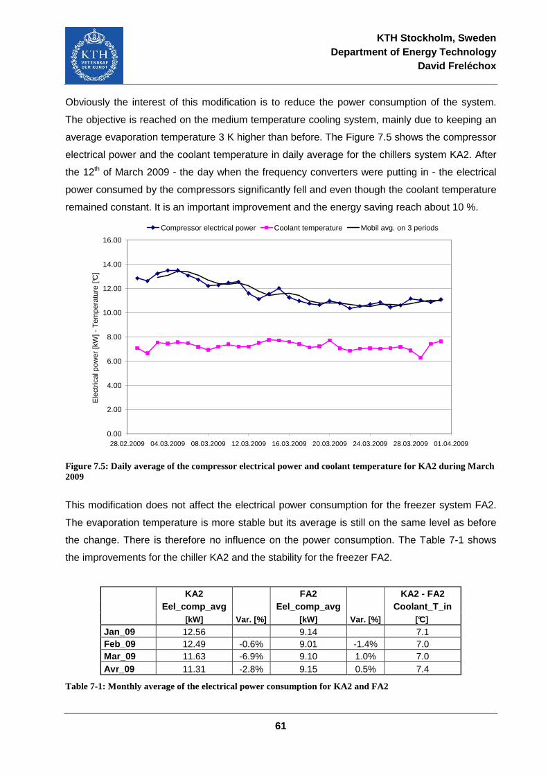
KTH Stockholm, Sweden Department of Energy Technology
David Freléchox
61
Obviously the interest of this modification is to reduce the power consumption of the system.
The objective is reached on the medium temperature cooling system, mainly due to keeping an
average evaporation temperature 3 K higher than before. The Figure 7.5 shows the compressor
electrical power and the coolant temperature in daily average for the chillers system KA2. After
the 12th of March 2009 - the day when the frequency converters were putting in - the electrical
power consumed by the compressors significantly fell and even though the coolant temperature
remained constant. It is an important improvement and the energy saving reach about 10 %.
0.00
2.00
4.00
6.00
8.00
10.00
12.00
14.00
16.00
28.02.2009 04.03.2009 08.03.2009 12.03.2009 16.03.2009 20.03.2009 24.03.2009 28.03.2009 01.04.2009
Ele
ctric
al p
ower
[kW
] - T
empe
ratu
re [°
C]
Compressor electrical power Coolant temperature Mobil avg. on 3 periods
Figure 7.5: Daily average of the compressor electrical power and coolant temperature for KA2 during March 2009
This modification does not affect the electrical power consumption for the freezer system FA2.
The evaporation temperature is more stable but its average is still on the same level as before
the change. There is therefore no influence on the power consumption. The Table 7-1 shows
the improvements for the chiller KA2 and the stability for the freezer FA2.
KA2 FA2 KA2 - FA2 Eel_comp_avg Eel_comp_avg Coolant_T_in
[kW] Var. [%] [kW] Var. [%] [°C]
Jan_09 12.56 9.14 7.1 Feb_09 12.49 -0.6% 9.01 -1.4% 7.0 Mar_09 11.63 -6.9% 9.10 1.0% 7.0 Avr_09 11.31 -2.8% 9.15 0.5% 7.4
Table 7-1: Monthly average of the electrical power consumption for KA2 and FA2
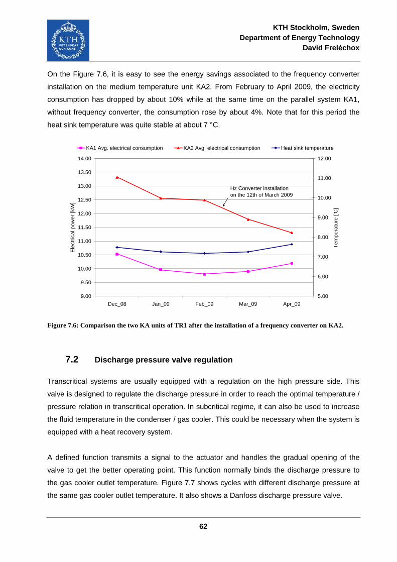
KTH Stockholm, Sweden Department of Energy Technology
David Freléchox
62
On the Figure 7.6, it is easy to see the energy savings associated to the frequency converter
installation on the medium temperature unit KA2. From February to April 2009, the electricity
consumption has dropped by about 10% while at the same time on the parallel system KA1,
without frequency converter, the consumption rose by about 4%. Note that for this period the
heat sink temperature was quite stable at about 7 °C.
9.00
9.50
10.00
10.50
11.00
11.50
12.00
12.50
13.00
13.50
14.00
Dec_08 Jan_09 Feb_09 Mar_09 Apr_09
Ele
ctric
al p
ower
[kW
]
5.00
6.00
7.00
8.00
9.00
10.00
11.00
12.00
Tem
pera
ture
[°C
]
KA1 Avg. electrical consumption KA2 Avg. electrical consumption Heat sink temperature
Hz Converter installationon the 12th of March 2009
Figure 7.6: Comparison the two KA units of TR1 after the installation of a frequency converter on KA2.
7.2 Discharge pressure valve regulation
Transcritical systems are usually equipped with a regulation on the high pressure side. This
valve is designed to regulate the discharge pressure in order to reach the optimal temperature /
pressure relation in transcritical operation. In subcritical regime, it can also be used to increase
the fluid temperature in the condenser / gas cooler. This could be necessary when the system is
equipped with a heat recovery system.
A defined function transmits a signal to the actuator and handles the gradual opening of the
valve to get the better operating point. This function normally binds the discharge pressure to
the gas cooler outlet temperature. Figure 7.7 shows cycles with different discharge pressure at
the same gas cooler outlet temperature. It also shows a Danfoss discharge pressure valve.
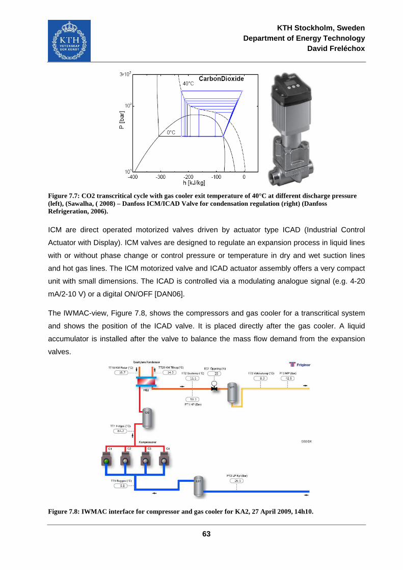
KTH Stockholm, Sweden Department of Energy Technology
David Freléchox
63
Figure 7.7: CO2 transcritical cycle with gas cooler exit temperature of 40°C at different discharge pressure (left), (Sawalha, ( 2008) – Danfoss ICM/ICAD Valve for condensation regulation (right) (Danfoss Refrigeration, 2006).
ICM are direct operated motorized valves driven by actuator type ICAD (Industrial Control
Actuator with Display). ICM valves are designed to regulate an expansion process in liquid lines
with or without phase change or control pressure or temperature in dry and wet suction lines
and hot gas lines. The ICM motorized valve and ICAD actuator assembly offers a very compact
unit with small dimensions. The ICAD is controlled via a modulating analogue signal (e.g. 4-20
mA/2-10 V) or a digital ON/OFF [DAN06].
The IWMAC-view, Figure 7.8, shows the compressors and gas cooler for a transcritical system
and shows the position of the ICAD valve. It is placed directly after the gas cooler. A liquid
accumulator is installed after the valve to balance the mass flow demand from the expansion
valves.
Figure 7.8: IWMAC interface for compressor and gas cooler for KA2, 27 April 2009, 14h10.
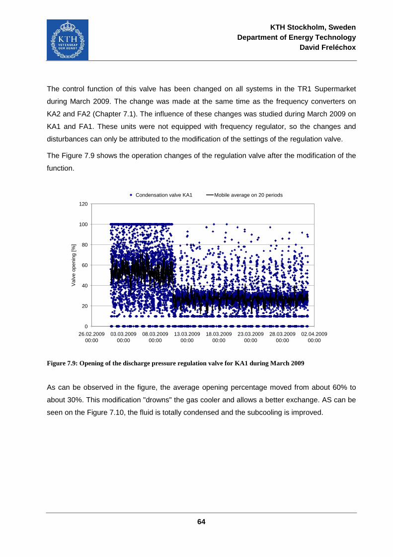
KTH Stockholm, Sweden Department of Energy Technology
David Freléchox
64
The control function of this valve has been changed on all systems in the TR1 Supermarket
during March 2009. The change was made at the same time as the frequency converters on
KA2 and FA2 (Chapter 7.1). The influence of these changes was studied during March 2009 on
KA1 and FA1. These units were not equipped with frequency regulator, so the changes and
disturbances can only be attributed to the modification of the settings of the regulation valve.
The Figure 7.9 shows the operation changes of the regulation valve after the modification of the
function.
0
20
40
60
80
100
120
26.02.200900:00
03.03.200900:00
08.03.200900:00
13.03.200900:00
18.03.200900:00
23.03.200900:00
28.03.200900:00
02.04.200900:00
Val
ve o
peni
ng [%
]
Condensation valve KA1 Mobile average on 20 periods
Figure 7.9: Opening of the discharge pressure regulation valve for KA1 during March 2009
As can be observed in the figure, the average opening percentage moved from about 60% to
about 30%. This modification "drowns" the gas cooler and allows a better exchange. AS can be
seen on the Figure 7.10, the fluid is totally condensed and the subcooling is improved.
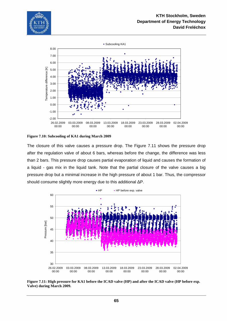
KTH Stockholm, Sweden Department of Energy Technology
David Freléchox
65
-2.00
-1.00
0.00
1.00
2.00
3.00
4.00
5.00
6.00
7.00
8.00
26.02.200900:00
03.03.200900:00
08.03.200900:00
13.03.200900:00
18.03.200900:00
23.03.200900:00
28.03.200900:00
02.04.200900:00
Tem
pera
ture
diff
eren
ce [K
]Subcooling KA1
Figure 7.10: Subcooling of KA1 during March 2009
The closure of this valve causes a pressure drop. The Figure 7.11 shows the pressure drop
after the regulation valve of about 6 bars, whereas before the change, the difference was less
than 2 bars. This pressure drop causes partial evaporation of liquid and causes the formation of
a liquid - gas mix in the liquid tank. Note that the partial closure of the valve causes a big
pressure drop but a minimal increase in the high pressure of about 1 bar. Thus, the compressor
should consume slightly more energy due to this additional ∆P.
30
35
40
45
50
55
60
26.02.200900:00
03.03.200900:00
08.03.200900:00
13.03.200900:00
18.03.200900:00
23.03.200900:00
28.03.200900:00
02.04.200900:00
Pre
ssur
e [b
ar]
HP HP before exp. valve
Figure 7.11: High pressure for KA1 before the ICAD valve (HP) and after the ICAD valve (HP before exp. Valve) during March 2009.
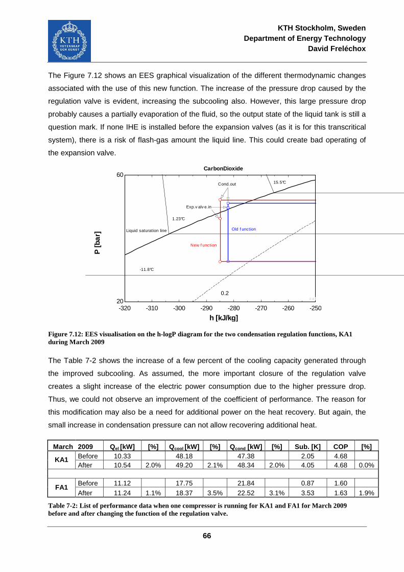
KTH Stockholm, Sweden Department of Energy Technology
David Freléchox
66
The Figure 7.12 shows an EES graphical visualization of the different thermodynamic changes
associated with the use of this new function. The increase of the pressure drop caused by the
regulation valve is evident, increasing the subcooling also. However, this large pressure drop
probably causes a partially evaporation of the fluid, so the output state of the liquid tank is still a
question mark. If none IHE is installed before the expansion valves (as it is for this transcritical
system), there is a risk of flash-gas amount the liquid line. This could create bad operating of
the expansion valve.
-320 -310 -300 -290 -280 -270 -260 -25020
60
h [kJ/kg]
P [b
ar]
15.5°C
1.23°C
-11.8°C
0.2 0.6 0.8
CarbonDioxide
Liquid saturation line Old f unction
New f unction
Cond.out
Exp.v alv e.in
Figure 7.12: EES visualisation on the h-logP diagram for the two condensation regulation functions, KA1 during March 2009
The Table 7-2 shows the increase of a few percent of the cooling capacity generated through
the improved subcooling. As assumed, the more important closure of the regulation valve
creates a slight increase of the electric power consumption due to the higher pressure drop.
Thus, we could not observe an improvement of the coefficient of performance. The reason for
this modification may also be a need for additional power on the heat recovery. But again, the
small increase in condensation pressure can not allow recovering additional heat.
March 2009 Qel [kW] [%] Q cool [kW] [%] Q cond [kW] [%] Sub. [K] COP [%] Before 10.33 48.18 47.38 2.05 4.68 KA1 After 10.54 2.0% 49.20 2.1% 48.34 2.0% 4.05 4.68 0.0%
Before 11.12 17.75 21.84 0.87 1.60
FA1 After 11.24 1.1% 18.37 3.5% 22.52 3.1% 3.53 1.63 1.9%
Table 7-2: List of performance data when one compressor is running for KA1 and FA1 for March 2009 before and after changing the function of the regulation valve.
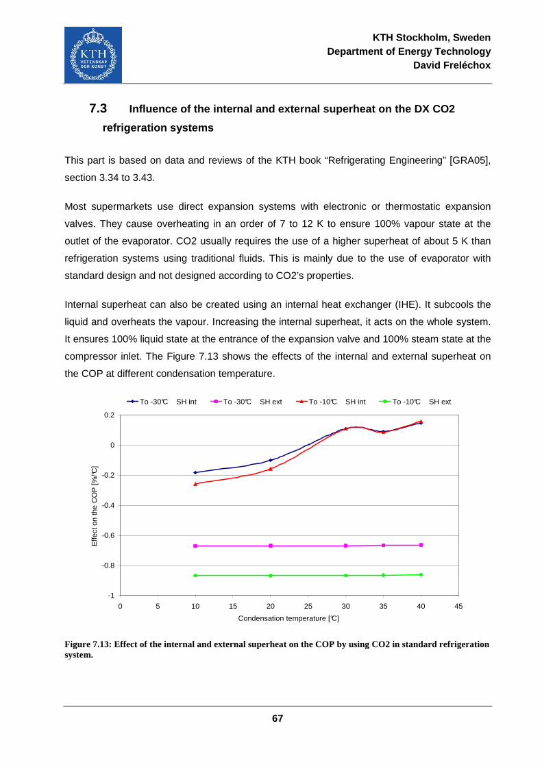
KTH Stockholm, Sweden Department of Energy Technology
David Freléchox
67
7.3 Influence of the internal and external superheat on the DX CO2
refrigeration systems
This part is based on data and reviews of the KTH book “Refrigerating Engineering” [GRA05],
section 3.34 to 3.43.
Most supermarkets use direct expansion systems with electronic or thermostatic expansion
valves. They cause overheating in an order of 7 to 12 K to ensure 100% vapour state at the
outlet of the evaporator. CO2 usually requires the use of a higher superheat of about 5 K than
refrigeration systems using traditional fluids. This is mainly due to the use of evaporator with
standard design and not designed according to CO2’s properties.
Internal superheat can also be created using an internal heat exchanger (IHE). It subcools the
liquid and overheats the vapour. Increasing the internal superheat, it acts on the whole system.
It ensures 100% liquid state at the entrance of the expansion valve and 100% steam state at the
compressor inlet. The Figure 7.13 shows the effects of the internal and external superheat on
the COP at different condensation temperature.
-1
-0.8
-0.6
-0.4
-0.2
0
0.2
0 5 10 15 20 25 30 35 40 45
Condensation temperature [°C]
Effe
ct o
n th
e C
OP
[%/°C
]
To -30°C _ SH int To -30°C _ SH ext To -10°C _ SH int To -10°C _ SH ext
Figure 7.13: Effect of the internal and external superheat on the COP by using CO2 in standard refrigeration system.
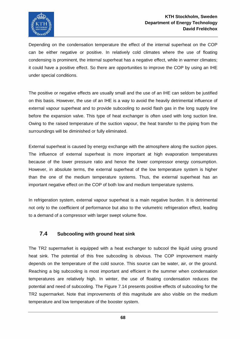
KTH Stockholm, Sweden Department of Energy Technology
David Freléchox
68
Depending on the condensation temperature the effect of the internal superheat on the COP
can be either negative or positive. In relatively cold climates where the use of floating
condensing is prominent, the internal superheat has a negative effect, while in warmer climates;
it could have a positive effect. So there are opportunities to improve the COP by using an IHE
under special conditions.
The positive or negative effects are usually small and the use of an IHE can seldom be justified
on this basis. However, the use of an IHE is a way to avoid the heavily detrimental influence of
external vapour superheat and to provide subcooling to avoid flash gas in the long supply line
before the expansion valve. This type of heat exchanger is often used with long suction line.
Owing to the raised temperature of the suction vapour, the heat transfer to the piping from the
surroundings will be diminished or fully eliminated.
External superheat is caused by energy exchange with the atmosphere along the suction pipes.
The influence of external superheat is more important at high evaporation temperatures
because of the lower pressure ratio and hence the lower compressor energy consumption.
However, in absolute terms, the external superheat of the low temperature system is higher
than the one of the medium temperature systems. Thus, the external superheat has an
important negative effect on the COP of both low and medium temperature systems.
In refrigeration system, external vapour superheat is a main negative burden. It is detrimental
not only to the coefficient of performance but also to the volumetric refrigeration effect, leading
to a demand of a compressor with larger swept volume flow.
7.4 Subcooling with ground heat sink
The TR2 supermarket is equipped with a heat exchanger to subcool the liquid using ground
heat sink. The potential of this free subcooling is obvious. The COP improvement mainly
depends on the temperature of the cold source. This source can be water, air, or the ground.
Reaching a big subcooling is most important and efficient in the summer when condensation
temperatures are relatively high. In winter, the use of floating condensation reduces the
potential and need of subcooling. The Figure 7.14 presents positive effects of subcooling for the
TR2 supermarket. Note that improvements of this magnitude are also visible on the medium
temperature and low temperature of the booster system.
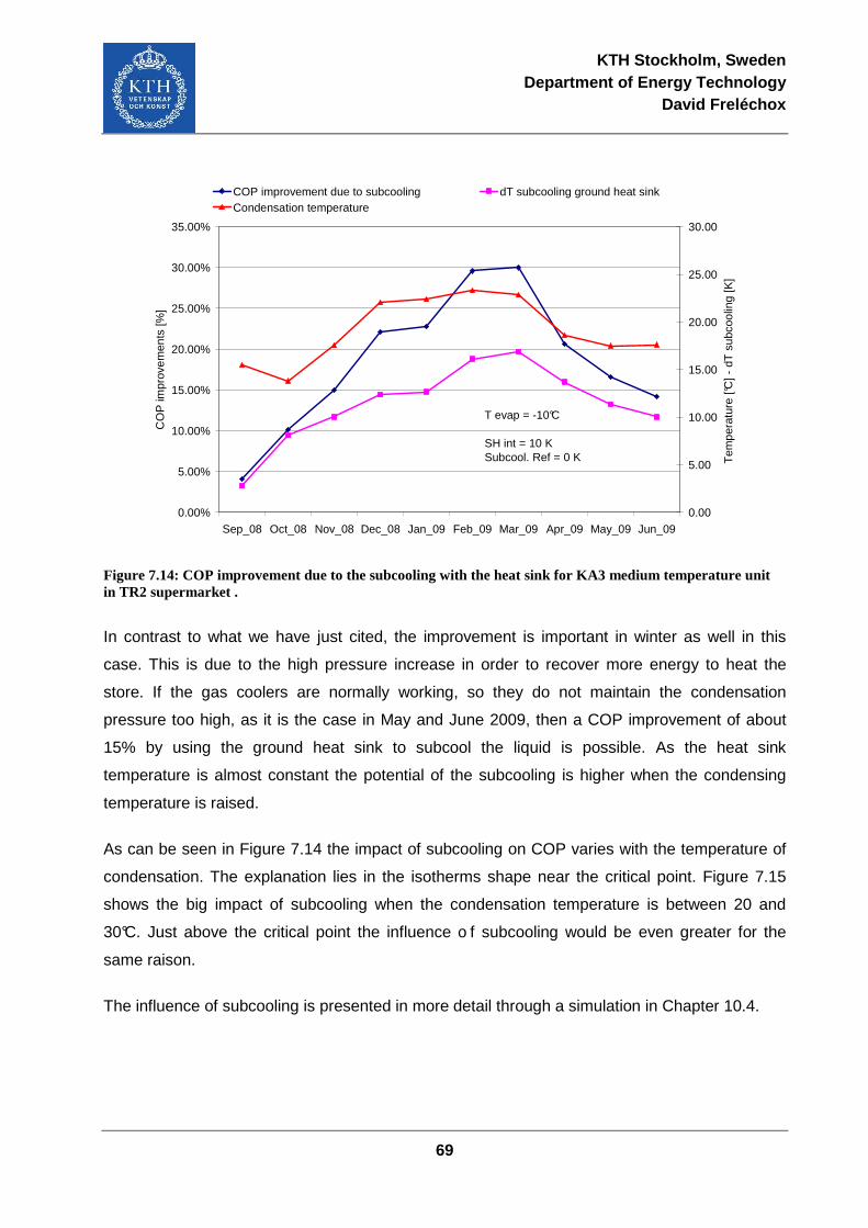
KTH Stockholm, Sweden Department of Energy Technology
David Freléchox
69
0.00%
5.00%
10.00%
15.00%
20.00%
25.00%
30.00%
35.00%
Sep_08 Oct_08 Nov_08 Dec_08 Jan_09 Feb_09 Mar_09 Apr_09 May_09 Jun_09
CO
P im
prov
emen
ts [%
]
0.00
5.00
10.00
15.00
20.00
25.00
30.00
Tem
pera
ture
[°C
] - d
T s
ubco
olin
g [K
]
COP improvement due to subcooling dT subcooling ground heat sinkCondensation temperature
T evap = -10°C
SH int = 10 KSubcool. Ref = 0 K
Figure 7.14: COP improvement due to the subcooling with the heat sink for KA3 medium temperature unit in TR2 supermarket .
In contrast to what we have just cited, the improvement is important in winter as well in this
case. This is due to the high pressure increase in order to recover more energy to heat the
store. If the gas coolers are normally working, so they do not maintain the condensation
pressure too high, as it is the case in May and June 2009, then a COP improvement of about
15% by using the ground heat sink to subcool the liquid is possible. As the heat sink
temperature is almost constant the potential of the subcooling is higher when the condensing
temperature is raised.
As can be seen in Figure 7.14 the impact of subcooling on COP varies with the temperature of
condensation. The explanation lies in the isotherms shape near the critical point. Figure 7.15
shows the big impact of subcooling when the condensation temperature is between 20 and
30°C. Just above the critical point the influence o f subcooling would be even greater for the
same raison.
The influence of subcooling is presented in more detail through a simulation in Chapter 10.4.

KTH Stockholm, Sweden Department of Energy Technology
David Freléchox
70
-300 -275 -250 -225 -200 -175 -150 -1253x101
102
102
h [kJ/kg]
P [b
ar]
30°C
25°C
20°C
15°C
10°C
CarbonDioxide
Figure 7.15: Isotherme shape in h-logP diagramm for CO2 near critical point
The impact of subcooling on systems using CO2 as fluid may also be a decisive advantage
compared to traditional fluids such as R404A. On Figure 7.16, it is easy to see that 1 K
subcooling give about 1% of COP improvement in the case of R404A. But it is not valid for CO2.
In this case, the influence of subcooling is more important and varies greatly depending on the
condensation temperature.
0.0%
10.0%
20.0%
30.0%
40.0%
50.0%
60.0%
0.00 2.00 4.00 6.00 8.00 10.00 12.00 14.00 16.00 18.00 20.00
Subcooling [K]
CO
P im
prov
emen
ts [%
]
CO2 - Tcond=20°C CO2 - Tcond=25°C CO2 - Tcond=30°C
R404A - Tcond=20°C R404A - Tcond=25°C R404A - Tcond=30°C
Tevap=-10°C
SH int = 10KSubcool. Ref. = 0 K
Figure 7.16: Effect on the COP of the subcooling at different condensation temperature for CO2 and R404A with an evaporation temperature at -10°C and an internal superheat of 10 K.
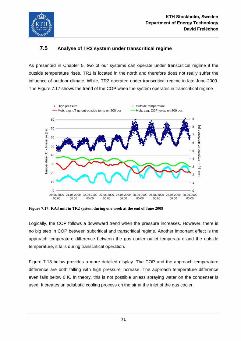
KTH Stockholm, Sweden Department of Energy Technology
David Freléchox
71
7.5 Analyse of TR2 system under transcritical regime
As presented in Chapter 5, two of our systems can operate under transcritical regime if the
outside temperature rises. TR1 is located in the north and therefore does not really suffer the
influence of outdoor climate. While, TR2 operated under transcritical regime in late June 2009.
The Figure 7.17 shows the trend of the COP when the system operates in transcritical regime
0
10
20
30
40
50
60
70
80
90
20.06.200900:00
21.06.200900:00
22.06.200900:00
23.06.200900:00
24.06.200900:00
25.06.200900:00
26.06.200900:00
27.06.200900:00
28.06.200900:00
Tem
pera
ture
[°C
] - P
ress
ure
[bar
]
0
1
2
3
4
5
6
7
8
9
10
CO
P [-
] - T
empe
ratu
re d
iffer
ence
[K]
High pressure Outside temperatureMob. avg. dT gc out-outside temp on 200 per Mob. avg. COP_evap on 200 per.
Figure 7.17: KA3 unit in TR2 system during one week at the end of June 2009
Logically, the COP follows a downward trend when the pressure increases. However, there is
no big step in COP between subcritical and transcritical regime. Another important effect is the
approach temperature difference between the gas cooler outlet temperature and the outside
temperature, it falls during transcritical operation.
Figure 7.18 below provides a more detailed display. The COP and the approach temperature
difference are both falling with high pressure increase. The approach temperature difference
even falls below 0 K. In theory, this is not possible unless spraying water on the condenser is
used. It creates an adiabatic cooling process on the air at the inlet of the gas cooler.
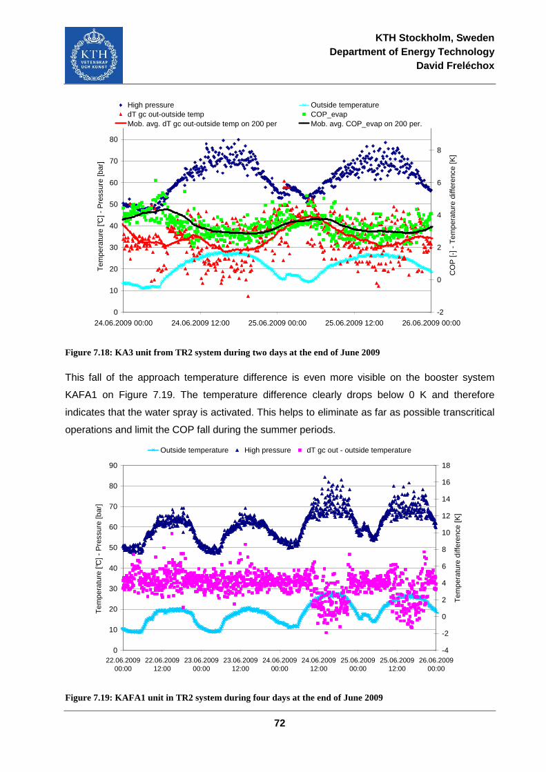
KTH Stockholm, Sweden Department of Energy Technology
David Freléchox
72
0
10
20
30
40
50
60
70
80
90
24.06.2009 00:00 24.06.2009 12:00 25.06.2009 00:00 25.06.2009 12:00 26.06.2009 00:00
Tem
pera
ture
[°C
] - P
ress
ure
[bar
]
-2
0
2
4
6
8
10
CO
P [-
] - T
empe
ratu
re d
iffer
ence
[K]
High pressure Outside temperaturedT gc out-outside temp COP_evapMob. avg. dT gc out-outside temp on 200 per Mob. avg. COP_evap on 200 per.
Figure 7.18: KA3 unit from TR2 system during two days at the end of June 2009
This fall of the approach temperature difference is even more visible on the booster system
KAFA1 on Figure 7.19. The temperature difference clearly drops below 0 K and therefore
indicates that the water spray is activated. This helps to eliminate as far as possible transcritical
operations and limit the COP fall during the summer periods.
0
10
20
30
40
50
60
70
80
90
22.06.200900:00
22.06.200912:00
23.06.200900:00
23.06.200912:00
24.06.200900:00
24.06.200912:00
25.06.200900:00
25.06.200912:00
26.06.200900:00
Tem
pera
ture
[°C
] - P
ress
ure
[bar
]
-4
-2
0
2
4
6
8
10
12
14
16
18T
empe
ratu
re d
iffer
ence
[K]
Outside temperature High pressure dT gc out - outside temperature
Figure 7.19: KAFA1 unit in TR2 system during four days at the end of June 2009
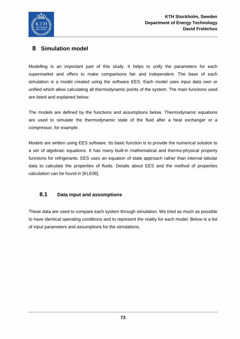
KTH Stockholm, Sweden Department of Energy Technology
David Freléchox
73
8 Simulation model
Modelling is an important part of this study. It helps to unify the parameters for each
supermarket and offers to make comparisons fair and independent. The base of each
simulation is a model created using the software EES. Each model uses input data own or
unified which allow calculating all thermodynamic points of the system. The main functions used
are listed and explained below.
The models are defined by the functions and assumptions below. Thermodynamic equations
are used to simulate the thermodynamic state of the fluid after a heat exchanger or a
compressor, for example.
Models are written using EES software. Its basic function is to provide the numerical solution to
a set of algebraic equations. It has many built-in mathematical and thermo-physical property
functions for refrigerants. EES uses an equation of state approach rather than internal tabular
data to calculate the properties of fluids. Details about EES and the method of properties
calculation can be found in [KLE06].
8.1 Data input and assomptions
These data are used to compare each system through simulation. We tried as much as possible
to have identical operating conditions and to represent the reality for each model. Below is a list
of input parameters and assumptions for the simulations.
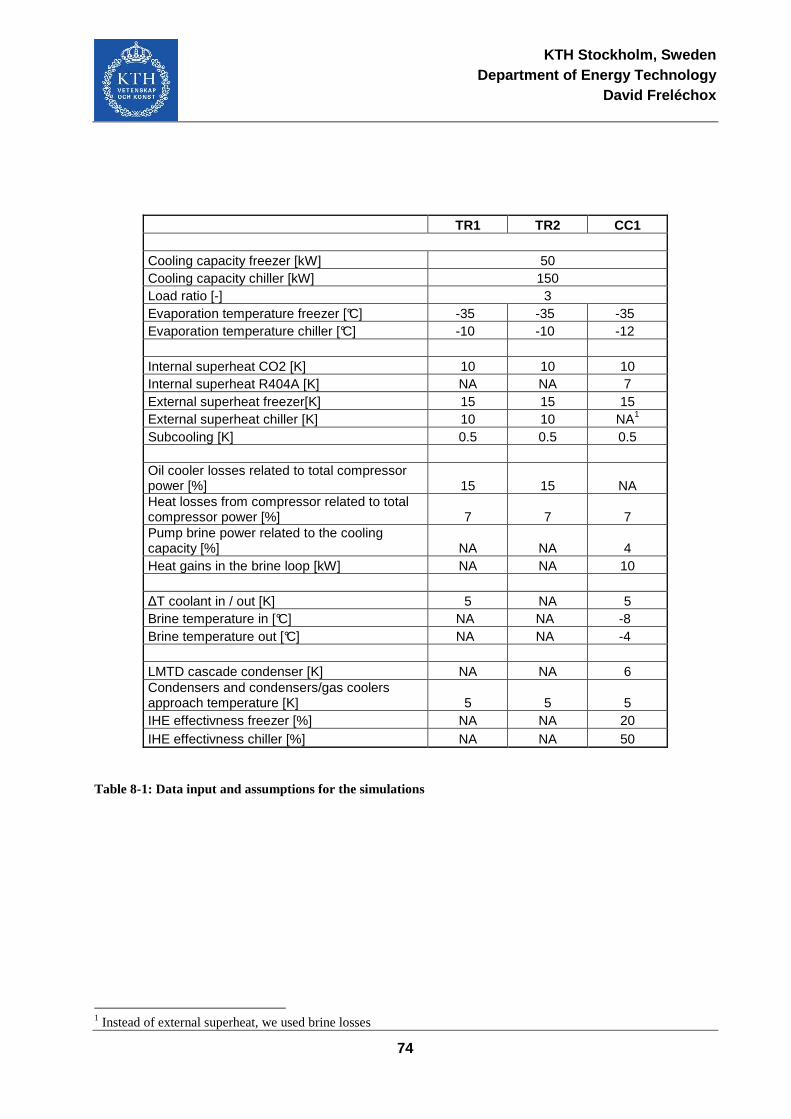
KTH Stockholm, Sweden Department of Energy Technology
David Freléchox
74
TR1 TR2 CC1 Cooling capacity freezer [kW] 50 Cooling capacity chiller [kW] 150 Load ratio [-] 3 Evaporation temperature freezer [°C] -35 -35 -35 Evaporation temperature chiller [°C] -10 -10 -12 Internal superheat CO2 [K] 10 10 10 Internal superheat R404A [K] NA NA 7 External superheat freezer[K] 15 15 15 External superheat chiller [K] 10 10 NA1 Subcooling [K] 0.5 0.5 0.5 Oil cooler losses related to total compressor power [%] 15 15 NA Heat losses from compressor related to total compressor power [%] 7 7 7 Pump brine power related to the cooling capacity [%] NA NA 4 Heat gains in the brine loop [kW] NA NA 10 ∆T coolant in / out [K] 5 NA 5 Brine temperature in [°C] NA NA -8 Brine temperature out [°C] NA NA -4 LMTD cascade condenser [K] NA NA 6 Condensers and condensers/gas coolers approach temperature [K] 5 5 5 IHE effectivness freezer [%] NA NA 20 IHE effectivness chiller [%] NA NA 50
Table 8-1: Data input and assumptions for the simulations
1 Instead of external superheat, we used brine losses
KTH Stockholm, Sweden Department of Energy Technology
David Freléchox
75
A load ratio of 3 was chosen as a representative value for Swedish supermarkets [SAW08]. The
refrigeration capacity is based on a mid-size supermarket with 50 kW for the low temperature
unit and 150 kW for the medium temperature unit [SAW08]. Evaporating temperature values are
recommended by cabinet manufacturers and used in most studies. Nevertheless, it appears
according to Girotto et al. (2005) that the use of higher temperatures evaporation of
approximately 2 K is possible with CO2. However, in order to produce a neutral study, we
decided to keep the standard values at -10°C and -3 5°C. They also correlate quite well with our
measurements in-situ.
Concerning the internal superheat, we remained in magnitudes and choose fixed values closer
to our measurements. Especially since these values depend on the configuration of each
system. The superheat of 7 K and the absence of external superheat for the R404A unit result
from the fact that this unit is a compact system.
The heat losses and the oil cooler losses are based on manufacturer’s data, as well as some
measures. They are a percentage of the compressors power consumption. Note that R404A
and CO2 compressors for the CC1 supermarket are not equipped with external oil cooler. The
power of the brine pumps is a percentage of the cooling capacity of the R404A unit. The values
are based on a study from E. Granryd (2007) and correlate with our measurements.
The effectiveness of heat exchangers and the logarithmic mean temperature difference are
based on our measurements and seem to be reasonable values. The temperature difference
between ambient air and the condenser/gas cooler outlet temperature is defined as the
approach temperature (in the case of a direct heat exchange air/CO2). Samer Sawalha
[SAW08] used 5 K, Girotto et al. [GIR04] 5 K as well, but they suggest the possibility of
improving the gas cooler and reach an approach temperature up to 2 K. A recent study by Ge et
al. [GEY09] uses 3 K. Our measurements on existing system give values between 4 and 5 K.
Finally, the value of 5 K was chosen as the most independent and realistic.
Ambient temperatures were logged for all the systems under investigation, A problem occurred
on the temperature sensors in CC1 supermarket and in order to have outside temperature for a
given period for the three systems, we use temperature data from Sveriges meteorologiska och
hydrologiska institute [SVE09] for the simulation. A weather station near each supermarket was
chosen as reference.
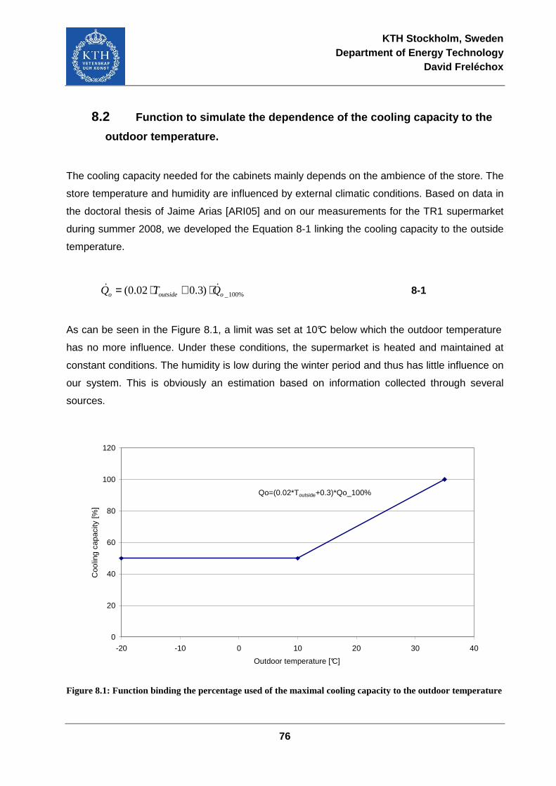
KTH Stockholm, Sweden Department of Energy Technology
David Freléchox
76
8.2 Function to simulate the dependence of the cooling capacity to the
outdoor temperature.
The cooling capacity needed for the cabinets mainly depends on the ambience of the store. The
store temperature and humidity are influenced by external climatic conditions. Based on data in
the doctoral thesis of Jaime Arias [ARI05] and on our measurements for the TR1 supermarket
during summer 2008, we developed the Equation 8-1 linking the cooling capacity to the outside
temperature.
%100_)3.002.0( ooutsideo QTQ && ⋅+⋅= 8-1
As can be seen in the Figure 8.1, a limit was set at 10°C below which the outdoor temperature
has no more influence. Under these conditions, the supermarket is heated and maintained at
constant conditions. The humidity is low during the winter period and thus has little influence on
our system. This is obviously an estimation based on information collected through several
sources.
0
20
40
60
80
100
120
-20 -10 0 10 20 30 40
Outdoor temperature [°C]
Coo
ling
capa
city
[%]
Qo=(0.02*Toutside+0.3)*Qo_100%
Figure 8.1: Function binding the percentage used of the maximal cooling capacity to the outdoor temperature
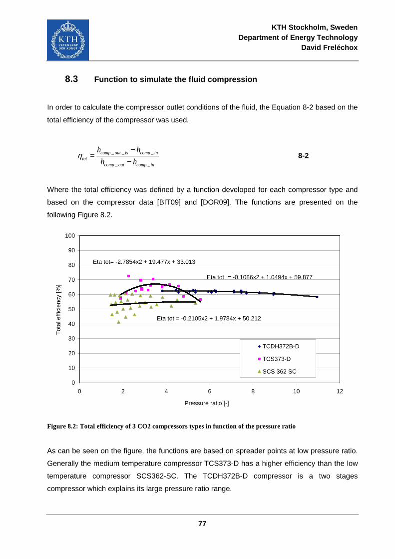
KTH Stockholm, Sweden Department of Energy Technology
David Freléchox
77
8.3 Function to simulate the fluid compression
In order to calculate the compressor outlet conditions of the fluid, the Equation 8-2 based on the
total efficiency of the compressor was used.
incompoutcomp
incompisoutcomptot hh
hh
__
___
−−
=η 8-2
Where the total efficiency was defined by a function developed for each compressor type and
based on the compressor data [BIT09] and [DOR09]. The functions are presented on the
following Figure 8.2.
Eta tot = -0.1086x2 + 1.0494x + 59.877
Eta tot= -2.7854x2 + 19.477x + 33.013
Eta tot = -0.2105x2 + 1.9784x + 50.212
0
10
20
30
40
50
60
70
80
90
100
0 2 4 6 8 10 12
Pressure ratio [-]
Tot
al e
ffici
ency
[%]
TCDH372B-D
TCS373-D
SCS 362 SC
Figure 8.2: Total efficiency of 3 CO2 compressors types in function of the pressure ratio
As can be seen on the figure, the functions are based on spreader points at low pressure ratio.
Generally the medium temperature compressor TCS373-D has a higher efficiency than the low
temperature compressor SCS362-SC. The TCDH372B-D compressor is a two stages
compressor which explains its large pressure ratio range.
KTH Stockholm, Sweden Department of Energy Technology
David Freléchox
78
8.4 Limit of the condensing temperature
The TR1 supermarket uses the floating condensation to limit the compressors power
consumption. The idea is to use the condenser capacity at the maximum to maintain the
condensing pressure as low as possible. The pressure ratio is lowered and compressors
consume less energy.
However, this method leads to technical constraints. Lowering the condensing temperature will
generally increase the cooling capacity and reduce the electrical energy consumed. Thus, it is
preferable to install a frequency converter on the compressor to continuously adapt its power,
and adjust the produced cooling capacity on the demand. If the pressure drop across the
expansion valve becomes too low, then its capacity goes down and there is a risk of under-
supply of refrigerant in the cabinets.
These constraints mean that there should be a minimum condensation temperature for each
system. The CO2 appears to have an advantage at this level regarding its high pressure
difference between low and high pressure (about 40 bars at -10°C +25°C). It should be possible
to lower the condensing temperature more than in the case of using traditional HFC, which are
working at lower pressure differences. For example, the R404A has a pressure difference of 8
bars between evaporation at -10°C and condensation at +25°C.
To fix a limit in our simulation model, we get contact with companies having experience in the
floating condensation field, for both CO2 and R404A. Regarding CO2, Micael Antonsson from
Green and Cool AB [ANT09] mentioned that it would be possible to work down to -5°C
condensation with evaporation at -10°C. The pressur e difference is still about 5 bars and this is
sufficient for proper functioning of the expansion valve. Nevertheless, there is a lack of
guarantee from compressors’ manufacturer at this low pressure difference. Long-term tests are
underway. Our measurements of both TR1 and TR2 supermarket indicate that condensation
temperatures are limited to 10 - 12°C.
KTH Stockholm, Sweden Department of Energy Technology
David Freléchox
79
Regarding R404A, Lasse Viktorsson from Partor AB indicates [VIK09] that it is possible to
achieve a condensation temperature of 5°C for mediu m temperature system and -5°C for low
temperature systems. An observation on the system in use from Partor AB indicates limit
condensation temperatures between 5 and 10 ° C.
The two contacts raised a warning that the lowest condensing temperature is not necessarily
the ideal energy wise. Indeed, there is an optimum for each system depending of its design and
its location between the energy saved and the additional electrical energy consumption by the
condenser fans. According to the measures and the diverse experiences of these companies,
floating condensing temperature limit lies at approximately 10°C for most installations in
Sweden.
With all this information and our measures, we finally decided to limit the temperature of
condensation of our model at 10°C.
8.5 Day and night influence on the cooling capacity
The differences between day and night are mainly du to the activity in the store, which suppose
an increase in humidity and temperature, the cabinet lights, the night curtains on medium
temperature cabinets and also the fill in of new products. All these parameters lead to an
increase in the cooling capacity demanded on the cabinets during the day.
This capacity variation can be more or less important depending on the store, the quality of its
ventilation and air conditioning system, number of its customers, its assortment of cabinets and
its management.
However, the difference between these two regimes is generally much larger on the medium
temperature system. The freezers are usually covered with lids or glass doors; it eliminates the
influence of the ambience on the low temperature system for a large degree.
The Figure 8.3 shows the day and night trends of the cooling capacity for medium temperature
unit in the TR1 supermarket during 10 days at the beginning of February 2009.
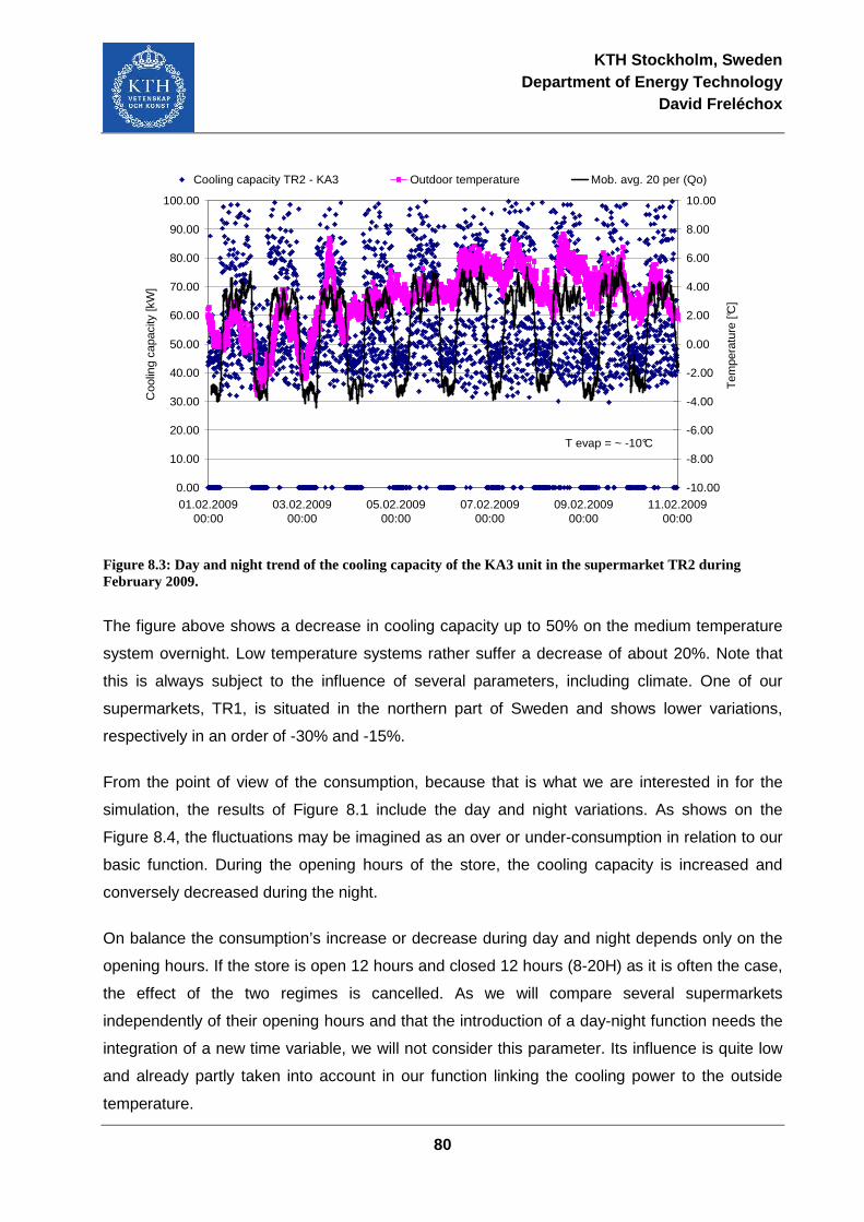
KTH Stockholm, Sweden Department of Energy Technology
David Freléchox
80
0.00
10.00
20.00
30.00
40.00
50.00
60.00
70.00
80.00
90.00
100.00
01.02.200900:00
03.02.200900:00
05.02.200900:00
07.02.200900:00
09.02.200900:00
11.02.200900:00
Coo
ling
capa
city
[kW
]
-10.00
-8.00
-6.00
-4.00
-2.00
0.00
2.00
4.00
6.00
8.00
10.00
Tem
pera
ture
[°C
]
Cooling capacity TR2 - KA3 Outdoor temperature Mob. avg. 20 per (Qo)
T evap = ~ -10°C
Figure 8.3: Day and night trend of the cooling capacity of the KA3 unit in the supermarket TR2 during February 2009.
The figure above shows a decrease in cooling capacity up to 50% on the medium temperature
system overnight. Low temperature systems rather suffer a decrease of about 20%. Note that
this is always subject to the influence of several parameters, including climate. One of our
supermarkets, TR1, is situated in the northern part of Sweden and shows lower variations,
respectively in an order of -30% and -15%.
From the point of view of the consumption, because that is what we are interested in for the
simulation, the results of Figure 8.1 include the day and night variations. As shows on the
Figure 8.4, the fluctuations may be imagined as an over or under-consumption in relation to our
basic function. During the opening hours of the store, the cooling capacity is increased and
conversely decreased during the night.
On balance the consumption’s increase or decrease during day and night depends only on the
opening hours. If the store is open 12 hours and closed 12 hours (8-20H) as it is often the case,
the effect of the two regimes is cancelled. As we will compare several supermarkets
independently of their opening hours and that the introduction of a day-night function needs the
integration of a new time variable, we will not consider this parameter. Its influence is quite low
and already partly taken into account in our function linking the cooling power to the outside
temperature.
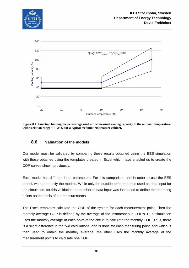
KTH Stockholm, Sweden Department of Energy Technology
David Freléchox
81
0
20
40
60
80
100
120
140
-20 -10 0 10 20 30 40
Outdoor temperature [°C]
Coo
ling
capa
city
[%]
Qo=(0.02*Toutside+0.3)*Qo_100%
Figure 8.4: Function binding the percentage used of the maximal cooling capacity to the outdoor temperature with variation range + / - 25% for a typical medium temperature cabinet.
8.6 Validation of the models
Our model must be validated by comparing these results obtained using the EES simulation
with those obtained using the templates created in Excel which have enabled us to create the
COP curves shown previously.
Each model has different input parameters. For this comparison and in order to use the EES
model, we had to unify the models. While only the outside temperature is used as data input for
the simulation, for this validation the number of data input was increased to define the operating
points on the basis of our measurements.
The Excel templates calculate the COP of the system for each measurement point. Then the
monthly average COP is defined by the average of the instantaneous COP’s. EES simulation
uses the monthly average of each point of the circuit to calculate the monthly COP. Thus, there
is a slight difference in the two calculations, one is done for each measuring point, and which is
then used to obtain the monthly average, the other uses the monthly average of the
measurement points to calculate one COP.
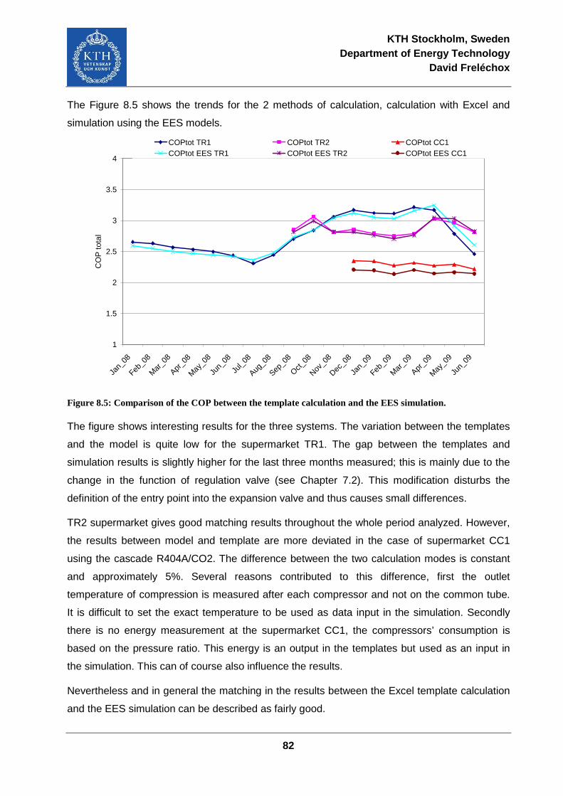
KTH Stockholm, Sweden Department of Energy Technology
David Freléchox
82
The Figure 8.5 shows the trends for the 2 methods of calculation, calculation with Excel and
simulation using the EES models.
1
1.5
2
2.5
3
3.5
4
Jan_
08
Feb_0
8
Mar
_08
Apr_0
8
May
_08
Jun_
08
Jul_0
8
Aug_0
8
Sep_0
8
Oct_08
Nov_0
8
Dec_0
8
Jan_
09
Feb_0
9
Mar
_09
Apr_0
9
May
_09
Jun_
09
CO
P to
tal
COPtot TR1 COPtot TR2 COPtot CC1 COPtot EES TR1 COPtot EES TR2 COPtot EES CC1
Figure 8.5: Comparison of the COP between the template calculation and the EES simulation.
The figure shows interesting results for the three systems. The variation between the templates
and the model is quite low for the supermarket TR1. The gap between the templates and
simulation results is slightly higher for the last three months measured; this is mainly due to the
change in the function of regulation valve (see Chapter 7.2). This modification disturbs the
definition of the entry point into the expansion valve and thus causes small differences.
TR2 supermarket gives good matching results throughout the whole period analyzed. However,
the results between model and template are more deviated in the case of supermarket CC1
using the cascade R404A/CO2. The difference between the two calculation modes is constant
and approximately 5%. Several reasons contributed to this difference, first the outlet
temperature of compression is measured after each compressor and not on the common tube.
It is difficult to set the exact temperature to be used as data input in the simulation. Secondly
there is no energy measurement at the supermarket CC1, the compressors’ consumption is
based on the pressure ratio. This energy is an output in the templates but used as an input in
the simulation. This can of course also influence the results.
Nevertheless and in general the matching in the results between the Excel template calculation
and the EES simulation can be described as fairly good.
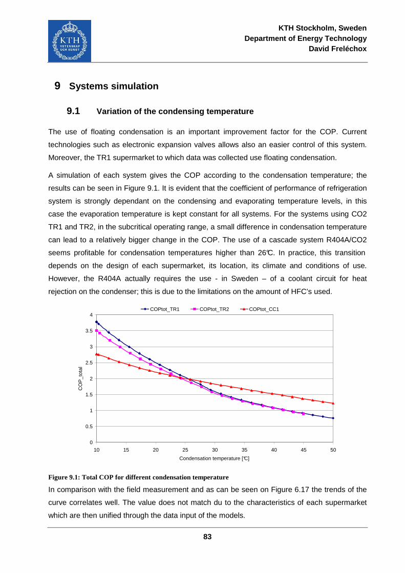
KTH Stockholm, Sweden Department of Energy Technology
David Freléchox
83
9 Systems simulation
9.1 Variation of the condensing temperature
The use of floating condensation is an important improvement factor for the COP. Current
technologies such as electronic expansion valves allows also an easier control of this system.
Moreover, the TR1 supermarket to which data was collected use floating condensation.
A simulation of each system gives the COP according to the condensation temperature; the
results can be seen in Figure 9.1. It is evident that the coefficient of performance of refrigeration
system is strongly dependant on the condensing and evaporating temperature levels, in this
case the evaporation temperature is kept constant for all systems. For the systems using CO2
TR1 and TR2, in the subcritical operating range, a small difference in condensation temperature
can lead to a relatively bigger change in the COP. The use of a cascade system R404A/CO2
seems profitable for condensation temperatures higher than 26°C. In practice, this transition
depends on the design of each supermarket, its location, its climate and conditions of use.
However, the R404A actually requires the use - in Sweden – of a coolant circuit for heat
rejection on the condenser; this is due to the limitations on the amount of HFC’s used.
0
0.5
1
1.5
2
2.5
3
3.5
4
10 15 20 25 30 35 40 45 50
Condensation temperature [°C]
CO
P_t
otal
COPtot_TR1 COPtot_TR2 COPtot_CC1
Figure 9.1: Total COP for different condensation temperature
In comparison with the field measurement and as can be seen on Figure 6.17 the trends of the
curve correlates well. The value does not match du to the characteristics of each supermarket
which are then unified through the data input of the models.
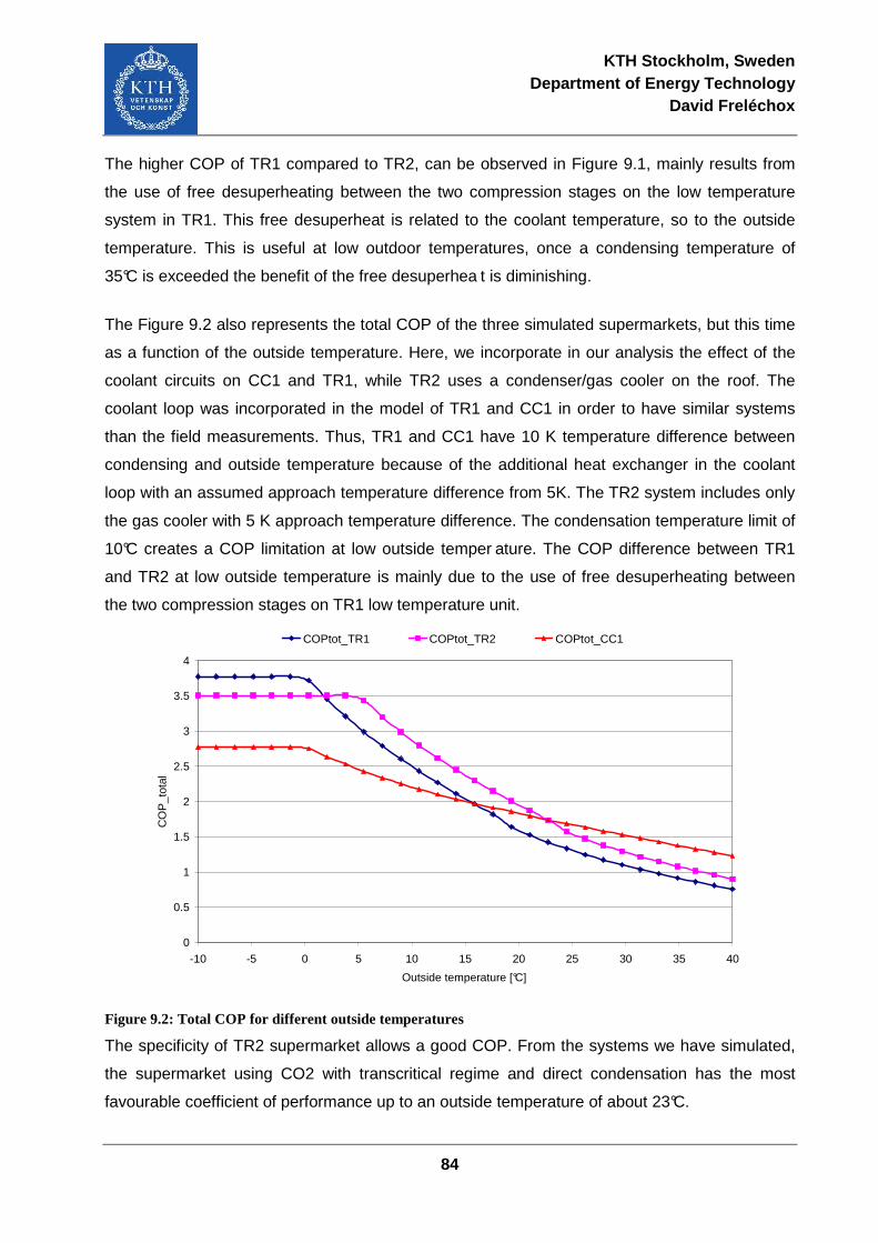
KTH Stockholm, Sweden Department of Energy Technology
David Freléchox
84
The higher COP of TR1 compared to TR2, can be observed in Figure 9.1, mainly results from
the use of free desuperheating between the two compression stages on the low temperature
system in TR1. This free desuperheat is related to the coolant temperature, so to the outside
temperature. This is useful at low outdoor temperatures, once a condensing temperature of
35°C is exceeded the benefit of the free desuperhea t is diminishing.
The Figure 9.2 also represents the total COP of the three simulated supermarkets, but this time
as a function of the outside temperature. Here, we incorporate in our analysis the effect of the
coolant circuits on CC1 and TR1, while TR2 uses a condenser/gas cooler on the roof. The
coolant loop was incorporated in the model of TR1 and CC1 in order to have similar systems
than the field measurements. Thus, TR1 and CC1 have 10 K temperature difference between
condensing and outside temperature because of the additional heat exchanger in the coolant
loop with an assumed approach temperature difference from 5K. The TR2 system includes only
the gas cooler with 5 K approach temperature difference. The condensation temperature limit of
10°C creates a COP limitation at low outside temper ature. The COP difference between TR1
and TR2 at low outside temperature is mainly due to the use of free desuperheating between
the two compression stages on TR1 low temperature unit.
0
0.5
1
1.5
2
2.5
3
3.5
4
-10 -5 0 5 10 15 20 25 30 35 40
Outside temperature [°C]
CO
P_t
otal
COPtot_TR1 COPtot_TR2 COPtot_CC1
Figure 9.2: Total COP for different outside temperatures
The specificity of TR2 supermarket allows a good COP. From the systems we have simulated,
the supermarket using CO2 with transcritical regime and direct condensation has the most
favourable coefficient of performance up to an outside temperature of about 23°C.
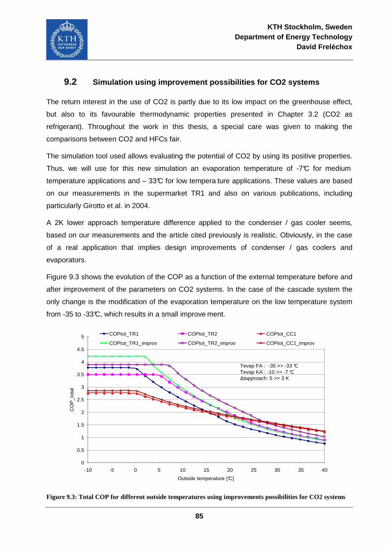
KTH Stockholm, Sweden Department of Energy Technology
David Freléchox
85
9.2 Simulation using improvement possibilities for CO2 systems
The return interest in the use of CO2 is partly due to its low impact on the greenhouse effect,
but also to its favourable thermodynamic properties presented in Chapter 3.2 (CO2 as
refrigerant). Throughout the work in this thesis, a special care was given to making the
comparisons between CO2 and HFCs fair.
The simulation tool used allows evaluating the potential of CO2 by using its positive properties.
Thus, we will use for this new simulation an evaporation temperature of -7°C for medium
temperature applications and – 33°C for low tempera ture applications. These values are based
on our measurements in the supermarket TR1 and also on various publications, including
particularly Girotto et al. in 2004.
A 2K lower approach temperature difference applied to the condenser / gas cooler seems,
based on our measurements and the article cited previously is realistic. Obviously, in the case
of a real application that implies design improvements of condenser / gas coolers and
evaporators.
Figure 9.3 shows the evolution of the COP as a function of the external temperature before and
after improvement of the parameters on CO2 systems. In the case of the cascade system the
only change is the modification of the evaporation temperature on the low temperature system
from -35 to -33°C, which results in a small improve ment.
0
0.5
1
1.5
2
2.5
3
3.5
4
4.5
5
-10 -5 0 5 10 15 20 25 30 35 40
Outside temperature [°C]
CO
P_t
otal
COPtot_TR1 COPtot_TR2 COPtot_CC1
COPtot_TR1_improv COPtot_TR2_improv COPtot_CC1_improv
Tevap FA : -35 >> -33 °CTevap KA : -10 >> -7 °C∆tapproach: 5 >> 3 K
Figure 9.3: Total COP for different outside temperatures using improvements possibilities for CO2 systems
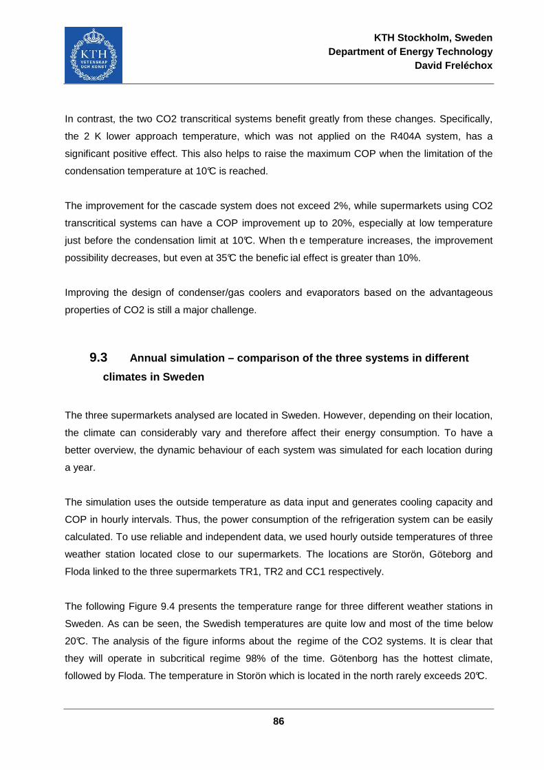
KTH Stockholm, Sweden Department of Energy Technology
David Freléchox
86
In contrast, the two CO2 transcritical systems benefit greatly from these changes. Specifically,
the 2 K lower approach temperature, which was not applied on the R404A system, has a
significant positive effect. This also helps to raise the maximum COP when the limitation of the
condensation temperature at 10°C is reached.
The improvement for the cascade system does not exceed 2%, while supermarkets using CO2
transcritical systems can have a COP improvement up to 20%, especially at low temperature
just before the condensation limit at 10°C. When th e temperature increases, the improvement
possibility decreases, but even at 35°C the benefic ial effect is greater than 10%.
Improving the design of condenser/gas coolers and evaporators based on the advantageous
properties of CO2 is still a major challenge.
9.3 Annual simulation – comparison of the three systems in different
climates in Sweden
The three supermarkets analysed are located in Sweden. However, depending on their location,
the climate can considerably vary and therefore affect their energy consumption. To have a
better overview, the dynamic behaviour of each system was simulated for each location during
a year.
The simulation uses the outside temperature as data input and generates cooling capacity and
COP in hourly intervals. Thus, the power consumption of the refrigeration system can be easily
calculated. To use reliable and independent data, we used hourly outside temperatures of three
weather station located close to our supermarkets. The locations are Storön, Göteborg and
Floda linked to the three supermarkets TR1, TR2 and CC1 respectively.
The following Figure 9.4 presents the temperature range for three different weather stations in
Sweden. As can be seen, the Swedish temperatures are quite low and most of the time below
20°C. The analysis of the figure informs about the regime of the CO2 systems. It is clear that
they will operate in subcritical regime 98% of the time. Götenborg has the hottest climate,
followed by Floda. The temperature in Storön which is located in the north rarely exceeds 20°C.
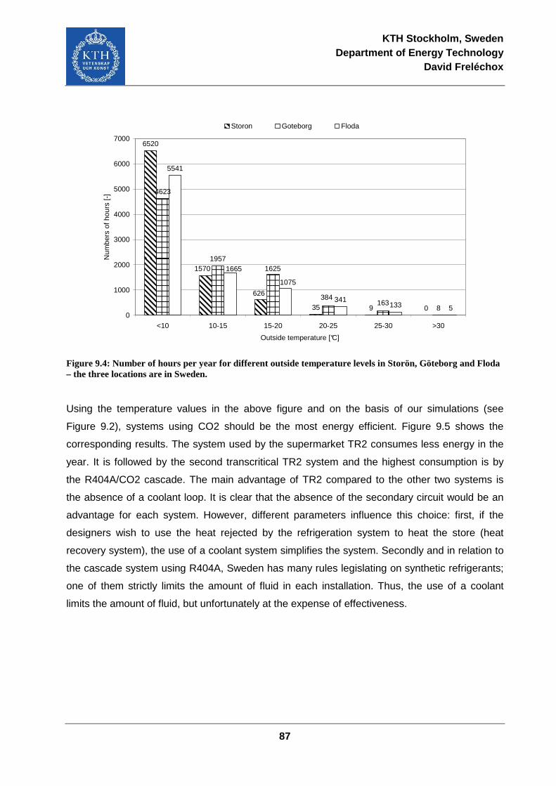
KTH Stockholm, Sweden Department of Energy Technology
David Freléchox
87
6520
35 9 0
4623
1957
8
5541
341133 5
626
1570
163384
1625
1075
1665
0
1000
2000
3000
4000
5000
6000
7000
<10 10-15 15-20 20-25 25-30 >30
Outside temperature [°C]
Num
bers
of h
ours
[-]
Storon Goteborg Floda
Figure 9.4: Number of hours per year for different outside temperature levels in Storön, Göteborg and Floda – the three locations are in Sweden.
Using the temperature values in the above figure and on the basis of our simulations (see
Figure 9.2), systems using CO2 should be the most energy efficient. Figure 9.5 shows the
corresponding results. The system used by the supermarket TR2 consumes less energy in the
year. It is followed by the second transcritical TR2 system and the highest consumption is by
the R404A/CO2 cascade. The main advantage of TR2 compared to the other two systems is
the absence of a coolant loop. It is clear that the absence of the secondary circuit would be an
advantage for each system. However, different parameters influence this choice: first, if the
designers wish to use the heat rejected by the refrigeration system to heat the store (heat
recovery system), the use of a coolant system simplifies the system. Secondly and in relation to
the cascade system using R404A, Sweden has many rules legislating on synthetic refrigerants;
one of them strictly limits the amount of fluid in each installation. Thus, the use of a coolant
limits the amount of fluid, but unfortunately at the expense of effectiveness.
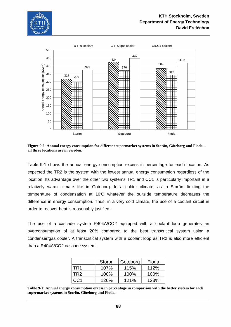
KTH Stockholm, Sweden Department of Energy Technology
David Freléchox
88
342
373
419
317
384
424
370
296
447
0
50
100
150
200
250
300
350
400
450
500
Storon Goteborg Floda
Ann
ual e
nerg
y co
nsum
ptio
n [M
Wh]
TR1 coolant TR2 gas cooler CC1 coolant
Figure 9.5: Annual energy consumption for different supermarket systems in Storön, Göteborg and Floda – all three locations are in Sweden.
Table 9-1 shows the annual energy consumption excess in percentage for each location. As
expected the TR2 is the system with the lowest annual energy consumption regardless of the
location. Its advantage over the other two systems TR1 and CC1 is particularly important in a
relatively warm climate like in Göteborg. In a colder climate, as in Storön, limiting the
temperature of condensation at 10°C whatever the ou tside temperature decreases the
difference in energy consumption. Thus, in a very cold climate, the use of a coolant circuit in
order to recover heat is reasonably justified.
The use of a cascade system R404A/CO2 equipped with a coolant loop generates an
overconsumption of at least 20% compared to the best transcritical system using a
condenser/gas cooler. A transcritical system with a coolant loop as TR2 is also more efficient
than a R404A/CO2 cascade system.
Storon Goteborg Floda TR1 107% 115% 112% TR2 100% 100% 100% CC1 126% 121% 123%
Table 9-1: Annual energy consumption excess in percentage in comparison with the better system for each supermarket systems in Storön, Göteborg and Floda.
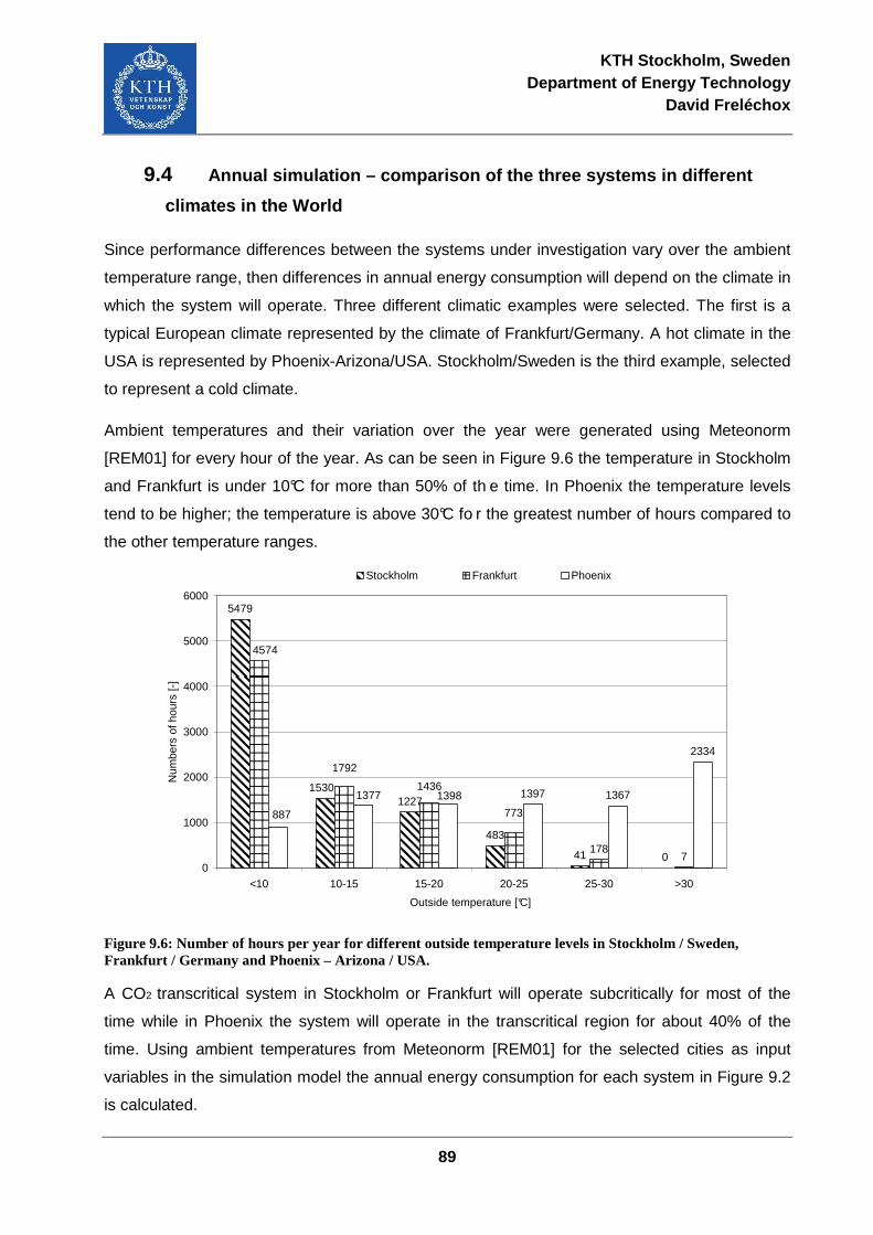
KTH Stockholm, Sweden Department of Energy Technology
David Freléchox
89
9.4 Annual simulation – comparison of the three systems in different
climates in the World
Since performance differences between the systems under investigation vary over the ambient
temperature range, then differences in annual energy consumption will depend on the climate in
which the system will operate. Three different climatic examples were selected. The first is a
typical European climate represented by the climate of Frankfurt/Germany. A hot climate in the
USA is represented by Phoenix-Arizona/USA. Stockholm/Sweden is the third example, selected
to represent a cold climate.
Ambient temperatures and their variation over the year were generated using Meteonorm
[REM01] for every hour of the year. As can be seen in Figure 9.6 the temperature in Stockholm
and Frankfurt is under 10°C for more than 50% of th e time. In Phoenix the temperature levels
tend to be higher; the temperature is above 30°C fo r the greatest number of hours compared to
the other temperature ranges.
5479
1227
483
41 0178
7
1397 1367
2334
1530
4574
773
1436
1792
13981377
887
0
1000
2000
3000
4000
5000
6000
<10 10-15 15-20 20-25 25-30 >30
Outside temperature [°C]
Num
bers
of h
ours
[-]
Stockholm Frankfurt Phoenix
Figure 9.6: Number of hours per year for different outside temperature levels in Stockholm / Sweden, Frankfurt / Germany and Phoenix – Arizona / USA.
A CO2 transcritical system in Stockholm or Frankfurt will operate subcritically for most of the
time while in Phoenix the system will operate in the transcritical region for about 40% of the
time. Using ambient temperatures from Meteonorm [REM01] for the selected cities as input
variables in the simulation model the annual energy consumption for each system in Figure 9.2
is calculated.
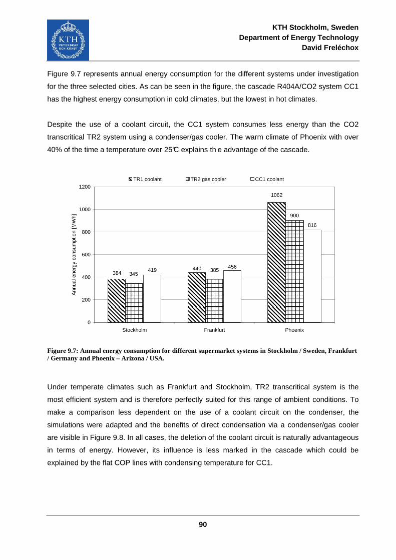
KTH Stockholm, Sweden Department of Energy Technology
David Freléchox
90
Figure 9.7 represents annual energy consumption for the different systems under investigation
for the three selected cities. As can be seen in the figure, the cascade R404A/CO2 system CC1
has the highest energy consumption in cold climates, but the lowest in hot climates.
Despite the use of a coolant circuit, the CC1 system consumes less energy than the CO2
transcritical TR2 system using a condenser/gas cooler. The warm climate of Phoenix with over
40% of the time a temperature over 25°C explains th e advantage of the cascade.
900
419
816
384
1062
440 385345
456
0
200
400
600
800
1000
1200
Stockholm Frankfurt Phoenix
Ann
ual e
nerg
y co
nsum
ptio
n [M
Wh]
TR1 coolant TR2 gas cooler CC1 coolant
Figure 9.7: Annual energy consumption for different supermarket systems in Stockholm / Sweden, Frankfurt / Germany and Phoenix – Arizona / USA.
Under temperate climates such as Frankfurt and Stockholm, TR2 transcritical system is the
most efficient system and is therefore perfectly suited for this range of ambient conditions. To
make a comparison less dependent on the use of a coolant circuit on the condenser, the
simulations were adapted and the benefits of direct condensation via a condenser/gas cooler
are visible in Figure 9.8. In all cases, the deletion of the coolant circuit is naturally advantageous
in terms of energy. However, its influence is less marked in the cascade which could be
explained by the flat COP lines with condensing temperature for CC1.
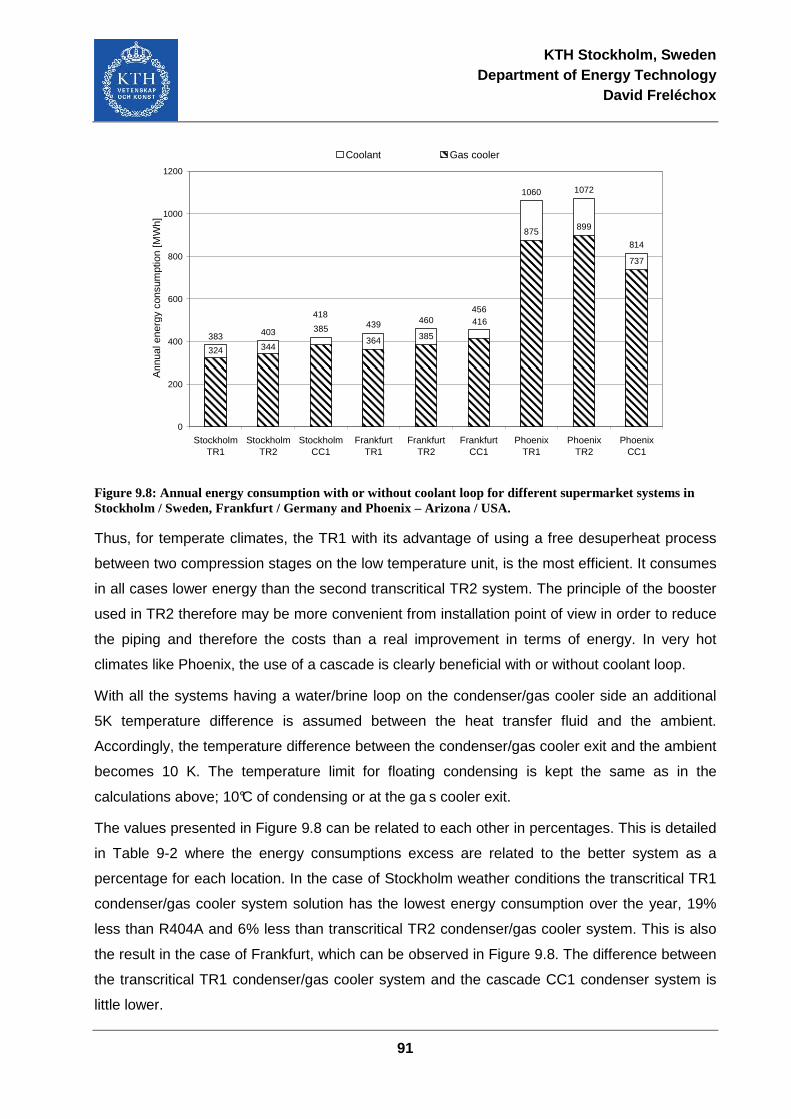
KTH Stockholm, Sweden Department of Energy Technology
David Freléchox
91
383 403439 460
1060 1072
814
364 385
875 899
737
456418
344324
416385
0
200
400
600
800
1000
1200
StockholmTR1
StockholmTR2
StockholmCC1
FrankfurtTR1
FrankfurtTR2
FrankfurtCC1
PhoenixTR1
PhoenixTR2
PhoenixCC1
Ann
ual e
nerg
y co
nsum
ptio
n [M
Wh]
Coolant Gas cooler
Figure 9.8: Annual energy consumption with or without coolant loop for different supermarket systems in Stockholm / Sweden, Frankfurt / Germany and Phoenix – Arizona / USA.
Thus, for temperate climates, the TR1 with its advantage of using a free desuperheat process
between two compression stages on the low temperature unit, is the most efficient. It consumes
in all cases lower energy than the second transcritical TR2 system. The principle of the booster
used in TR2 therefore may be more convenient from installation point of view in order to reduce
the piping and therefore the costs than a real improvement in terms of energy. In very hot
climates like Phoenix, the use of a cascade is clearly beneficial with or without coolant loop.
With all the systems having a water/brine loop on the condenser/gas cooler side an additional
5K temperature difference is assumed between the heat transfer fluid and the ambient.
Accordingly, the temperature difference between the condenser/gas cooler exit and the ambient
becomes 10 K. The temperature limit for floating condensing is kept the same as in the
calculations above; 10°C of condensing or at the ga s cooler exit.
The values presented in Figure 9.8 can be related to each other in percentages. This is detailed
in Table 9-2 where the energy consumptions excess are related to the better system as a
percentage for each location. In the case of Stockholm weather conditions the transcritical TR1
condenser/gas cooler system solution has the lowest energy consumption over the year, 19%
less than R404A and 6% less than transcritical TR2 condenser/gas cooler system. This is also
the result in the case of Frankfurt, which can be observed in Figure 9.8. The difference between
the transcritical TR1 condenser/gas cooler system and the cascade CC1 condenser system is
little lower.
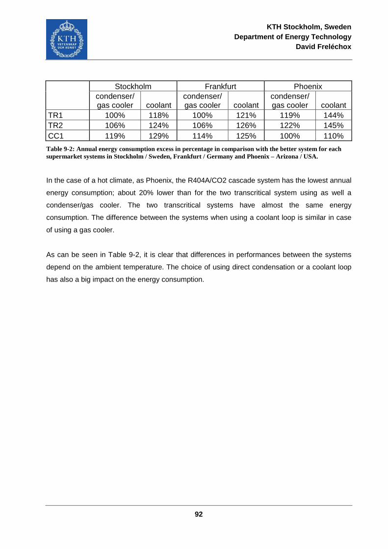
KTH Stockholm, Sweden Department of Energy Technology
David Freléchox
92
Stockholm Frankfurt Phoenix
condenser/ gas cooler coolant
condenser/ gas cooler coolant
condenser/ gas cooler coolant
TR1 100% 118% 100% 121% 119% 144% TR2 106% 124% 106% 126% 122% 145% CC1 119% 129% 114% 125% 100% 110%
Table 9-2: Annual energy consumption excess in percentage in comparison with the better system for each supermarket systems in Stockholm / Sweden, Frankfurt / Germany and Phoenix – Arizona / USA.
In the case of a hot climate, as Phoenix, the R404A/CO2 cascade system has the lowest annual
energy consumption; about 20% lower than for the two transcritical system using as well a
condenser/gas cooler. The two transcritical systems have almost the same energy
consumption. The difference between the systems when using a coolant loop is similar in case
of using a gas cooler.
As can be seen in Table 9-2, it is clear that differences in performances between the systems
depend on the ambient temperature. The choice of using direct condensation or a coolant loop
has also a big impact on the energy consumption.
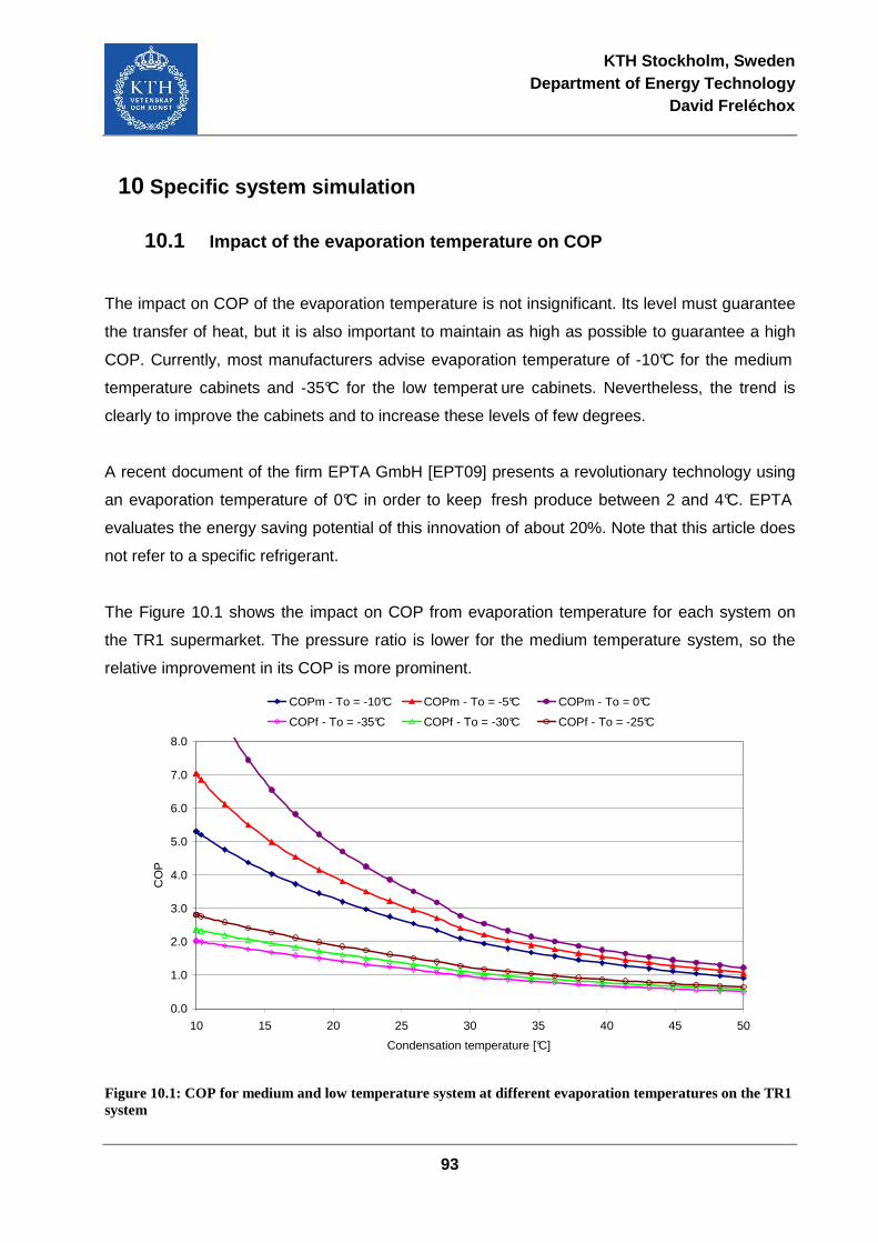
KTH Stockholm, Sweden Department of Energy Technology
David Freléchox
93
10 Specific system simulation
10.1 Impact of the evaporation temperature on COP
The impact on COP of the evaporation temperature is not insignificant. Its level must guarantee
the transfer of heat, but it is also important to maintain as high as possible to guarantee a high
COP. Currently, most manufacturers advise evaporation temperature of -10°C for the medium
temperature cabinets and -35°C for the low temperat ure cabinets. Nevertheless, the trend is
clearly to improve the cabinets and to increase these levels of few degrees.
A recent document of the firm EPTA GmbH [EPT09] presents a revolutionary technology using
an evaporation temperature of 0°C in order to keep fresh produce between 2 and 4°C. EPTA
evaluates the energy saving potential of this innovation of about 20%. Note that this article does
not refer to a specific refrigerant.
The Figure 10.1 shows the impact on COP from evaporation temperature for each system on
the TR1 supermarket. The pressure ratio is lower for the medium temperature system, so the
relative improvement in its COP is more prominent.
0.0
1.0
2.0
3.0
4.0
5.0
6.0
7.0
8.0
10 15 20 25 30 35 40 45 50
Condensation temperature [°C]
CO
P
COPm - To = -10°C COPm - To = -5°C COPm - To = 0°C
COPf - To = -35°C COPf - To = -30°C COPf - To = -25°C
Figure 10.1: COP for medium and low temperature system at different evaporation temperatures on the TR1 system
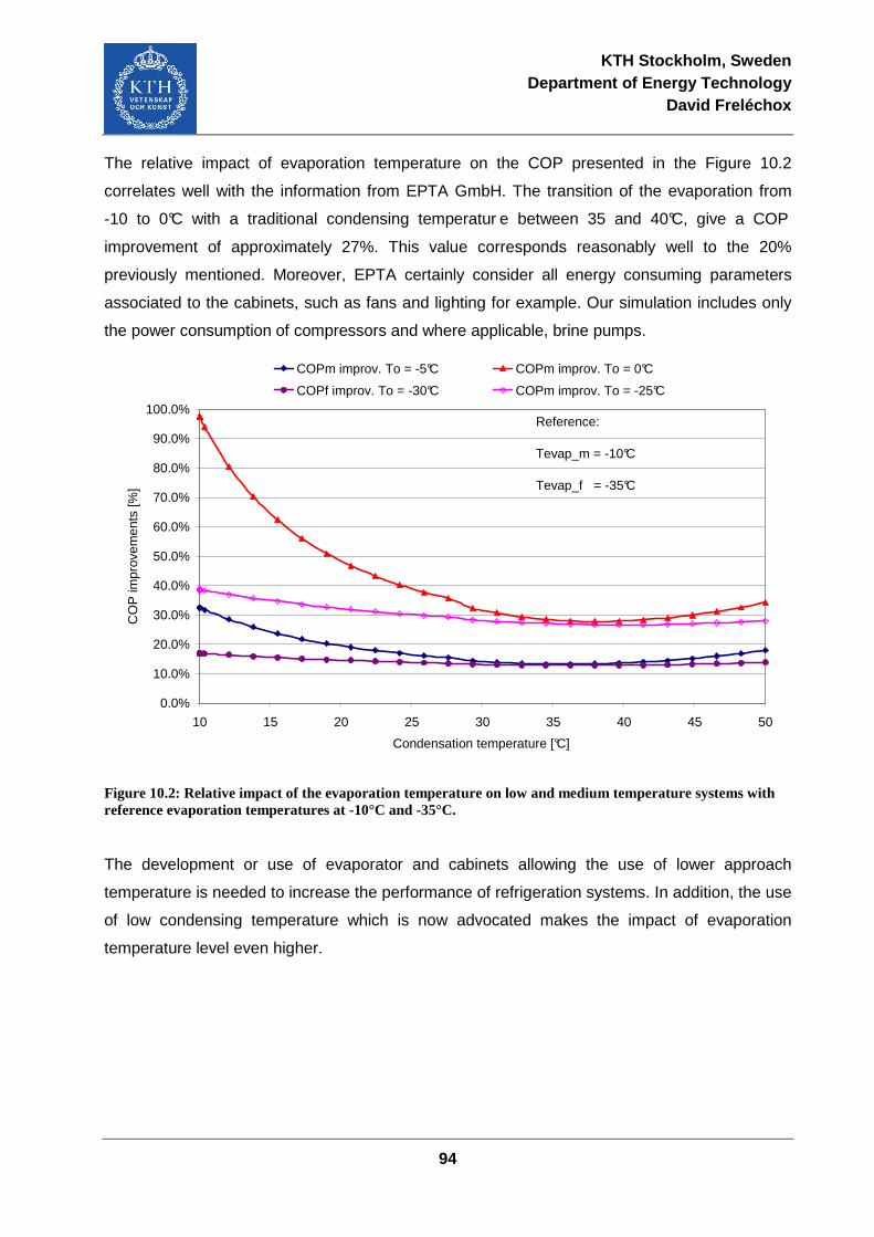
KTH Stockholm, Sweden Department of Energy Technology
David Freléchox
94
The relative impact of evaporation temperature on the COP presented in the Figure 10.2
correlates well with the information from EPTA GmbH. The transition of the evaporation from
-10 to 0°C with a traditional condensing temperatur e between 35 and 40°C, give a COP
improvement of approximately 27%. This value corresponds reasonably well to the 20%
previously mentioned. Moreover, EPTA certainly consider all energy consuming parameters
associated to the cabinets, such as fans and lighting for example. Our simulation includes only
the power consumption of compressors and where applicable, brine pumps.
0.0%
10.0%
20.0%
30.0%
40.0%
50.0%
60.0%
70.0%
80.0%
90.0%
100.0%
10 15 20 25 30 35 40 45 50
Condensation temperature [°C]
CO
P im
prov
emen
ts [%
]
COPm improv. To = -5°C COPm improv. To = 0°C
COPf improv. To = -30°C COPm improv. To = -25°C
Reference:
Tevap_m = -10°C
Tevap_f = -35°C
Figure 10.2: Relative impact of the evaporation temperature on low and medium temperature systems with reference evaporation temperatures at -10°C and -35°C.
The development or use of evaporator and cabinets allowing the use of lower approach
temperature is needed to increase the performance of refrigeration systems. In addition, the use
of low condensing temperature which is now advocated makes the impact of evaporation
temperature level even higher.
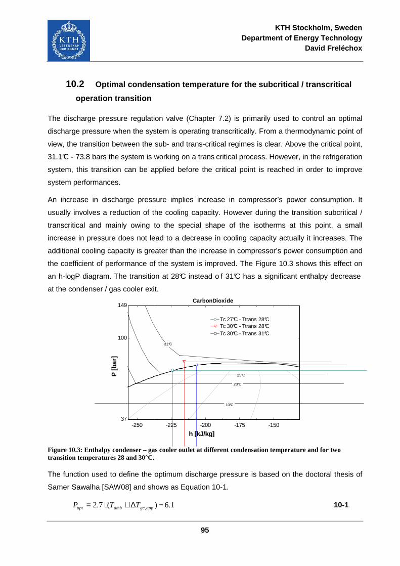
KTH Stockholm, Sweden Department of Energy Technology
David Freléchox
95
10.2 Optimal condensation temperature for the subcritica l / transcritical
operation transition
The discharge pressure regulation valve (Chapter 7.2) is primarily used to control an optimal
discharge pressure when the system is operating transcritically. From a thermodynamic point of
view, the transition between the sub- and trans-critical regimes is clear. Above the critical point,
31.1°C - 73.8 bars the system is working on a trans critical process. However, in the refrigeration
system, this transition can be applied before the critical point is reached in order to improve
system performances.
An increase in discharge pressure implies increase in compressor’s power consumption. It
usually involves a reduction of the cooling capacity. However during the transition subcritical /
transcritical and mainly owing to the special shape of the isotherms at this point, a small
increase in pressure does not lead to a decrease in cooling capacity actually it increases. The
additional cooling capacity is greater than the increase in compressor’s power consumption and
the coefficient of performance of the system is improved. The Figure 10.3 shows this effect on
an h-logP diagram. The transition at 28°C instead o f 31°C has a significant enthalpy decrease
at the condenser / gas cooler exit.
-250 -225 -200 -175 -15037
100
149
h [kJ/kg]
P [b
ar]
10°C
20°C
25°C
31°C
CarbonDioxide
Tc 27°C - Ttrans 28°CTc 27°C - Ttrans 28°C
Tc 30°C - Ttrans 31°CTc 30°C - Ttrans 31°CTc 30°C - Ttrans 28°CTc 30°C - Ttrans 28°C
Figure 10.3: Enthalpy condenser – gas cooler outlet at different condensation temperature and for two transition temperatures 28 and 30°C.
The function used to define the optimum discharge pressure is based on the doctoral thesis of
Samer Sawalha [SAW08] and shows as Equation 10-1.
1.6)(7.2 , −∆+⋅= appgcambopt TTP 10-1
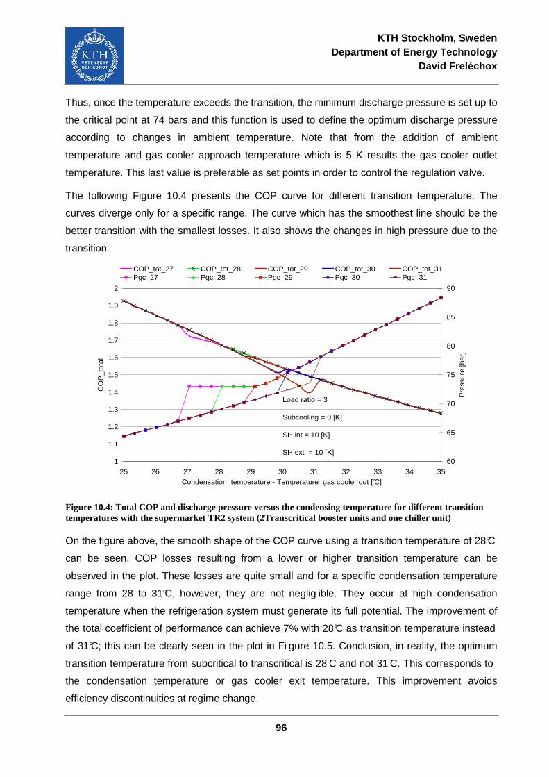
KTH Stockholm, Sweden Department of Energy Technology
David Freléchox
96
Thus, once the temperature exceeds the transition, the minimum discharge pressure is set up to
the critical point at 74 bars and this function is used to define the optimum discharge pressure
according to changes in ambient temperature. Note that from the addition of ambient
temperature and gas cooler approach temperature which is 5 K results the gas cooler outlet
temperature. This last value is preferable as set points in order to control the regulation valve.
The following Figure 10.4 presents the COP curve for different transition temperature. The
curves diverge only for a specific range. The curve which has the smoothest line should be the
better transition with the smallest losses. It also shows the changes in high pressure due to the
transition.
1
1.1
1.2
1.3
1.4
1.5
1.6
1.7
1.8
1.9
2
25 26 27 28 29 30 31 32 33 34 35Condensation temperature - Temperature gas cooler out [°C]
CO
P_t
otal
60
65
70
75
80
85
90
Pre
ssur
e [b
ar]
COP_tot_27 COP_tot_28 COP_tot_29 COP_tot_30 COP_tot_31Pgc_27 Pgc_28 Pgc_29 Pgc_30 Pgc_31
Load ratio = 3
Subcooling = 0 [K]
SH int = 10 [K]
SH ext = 10 [K]
Figure 10.4: Total COP and discharge pressure versus the condensing temperature for different transition temperatures with the supermarket TR2 system (2Transcritical booster units and one chiller unit)
On the figure above, the smooth shape of the COP curve using a transition temperature of 28°C
can be seen. COP losses resulting from a lower or higher transition temperature can be
observed in the plot. These losses are quite small and for a specific condensation temperature
range from 28 to 31°C, however, they are not neglig ible. They occur at high condensation
temperature when the refrigeration system must generate its full potential. The improvement of
the total coefficient of performance can achieve 7% with 28°C as transition temperature instead
of 31°C; this can be clearly seen in the plot in Fi gure 10.5. Conclusion, in reality, the optimum
transition temperature from subcritical to transcritical is 28°C and not 31°C. This corresponds to
the condensation temperature or gas cooler exit temperature. This improvement avoids
efficiency discontinuities at regime change.
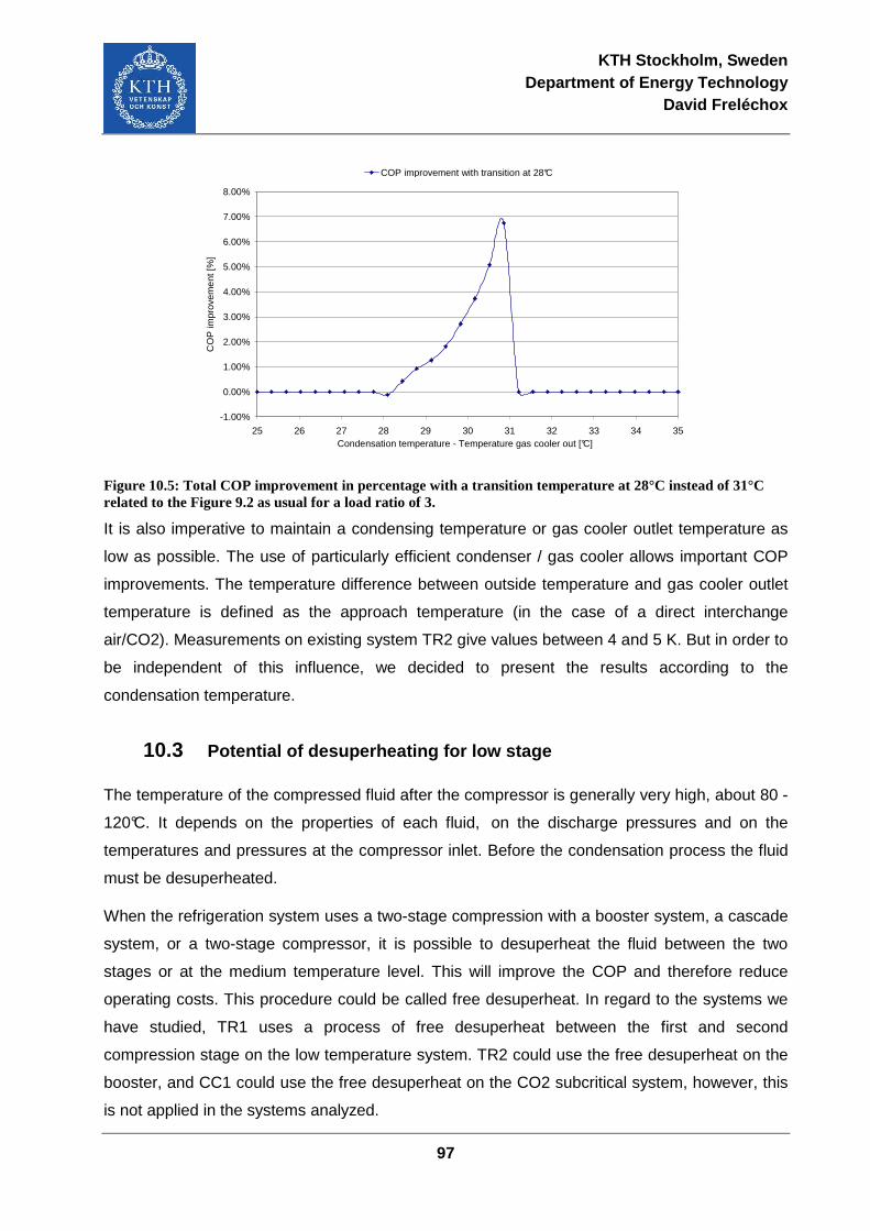
KTH Stockholm, Sweden Department of Energy Technology
David Freléchox
97
-1.00%
0.00%
1.00%
2.00%
3.00%
4.00%
5.00%
6.00%
7.00%
8.00%
25 26 27 28 29 30 31 32 33 34 35Condensation temperature - Temperature gas cooler out [°C]
CO
P im
prov
emen
t [%
]
COP improvement with transition at 28°C
Figure 10.5: Total COP improvement in percentage with a transition temperature at 28°C instead of 31°C related to the Figure 9.2 as usual for a load ratio of 3.
It is also imperative to maintain a condensing temperature or gas cooler outlet temperature as
low as possible. The use of particularly efficient condenser / gas cooler allows important COP
improvements. The temperature difference between outside temperature and gas cooler outlet
temperature is defined as the approach temperature (in the case of a direct interchange
air/CO2). Measurements on existing system TR2 give values between 4 and 5 K. But in order to
be independent of this influence, we decided to present the results according to the
condensation temperature.
10.3 Potential of desuperheating for low stage
The temperature of the compressed fluid after the compressor is generally very high, about 80 -
120°C. It depends on the properties of each fluid, on the discharge pressures and on the
temperatures and pressures at the compressor inlet. Before the condensation process the fluid
must be desuperheated.
When the refrigeration system uses a two-stage compression with a booster system, a cascade
system, or a two-stage compressor, it is possible to desuperheat the fluid between the two
stages or at the medium temperature level. This will improve the COP and therefore reduce
operating costs. This procedure could be called free desuperheat. In regard to the systems we
have studied, TR1 uses a process of free desuperheat between the first and second
compression stage on the low temperature system. TR2 could use the free desuperheat on the
booster, and CC1 could use the free desuperheat on the CO2 subcritical system, however, this
is not applied in the systems analyzed.
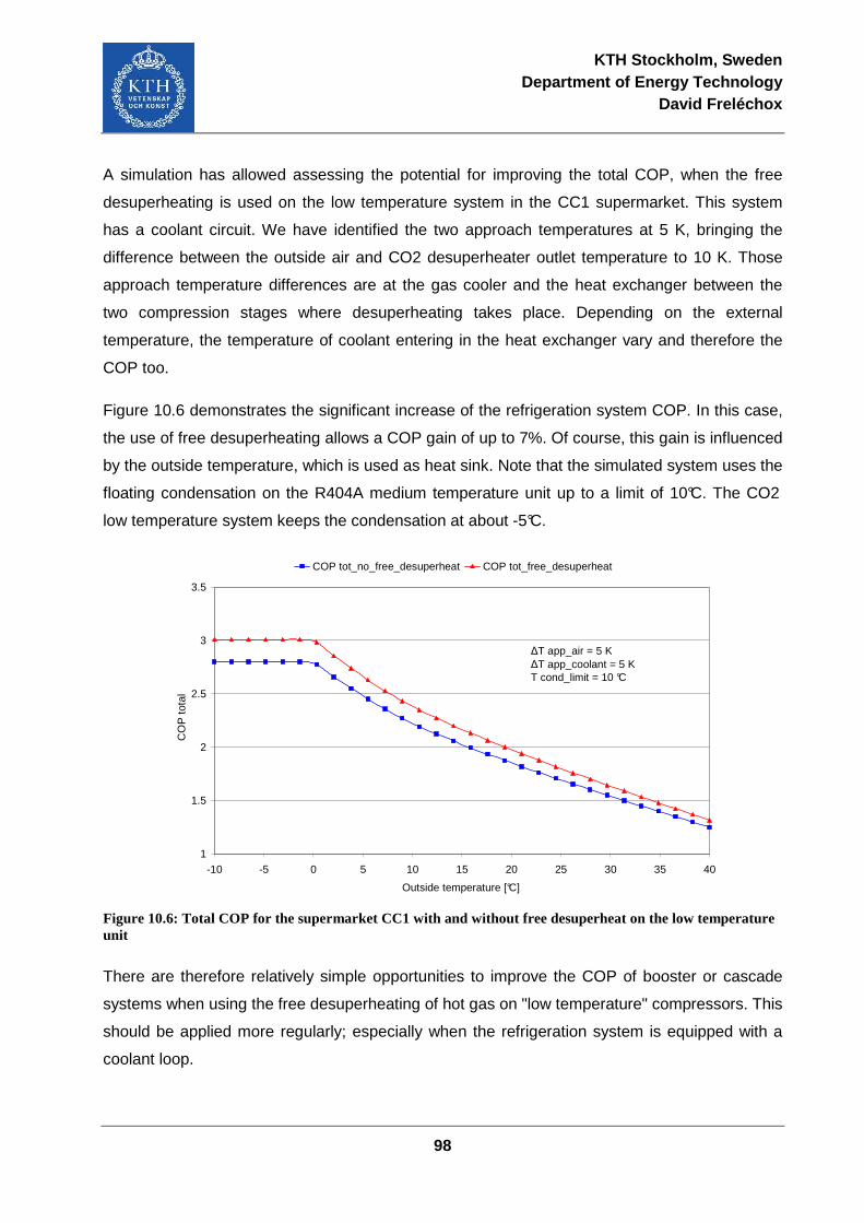
KTH Stockholm, Sweden Department of Energy Technology
David Freléchox
98
A simulation has allowed assessing the potential for improving the total COP, when the free
desuperheating is used on the low temperature system in the CC1 supermarket. This system
has a coolant circuit. We have identified the two approach temperatures at 5 K, bringing the
difference between the outside air and CO2 desuperheater outlet temperature to 10 K. Those
approach temperature differences are at the gas cooler and the heat exchanger between the
two compression stages where desuperheating takes place. Depending on the external
temperature, the temperature of coolant entering in the heat exchanger vary and therefore the
COP too.
Figure 10.6 demonstrates the significant increase of the refrigeration system COP. In this case,
the use of free desuperheating allows a COP gain of up to 7%. Of course, this gain is influenced
by the outside temperature, which is used as heat sink. Note that the simulated system uses the
floating condensation on the R404A medium temperature unit up to a limit of 10°C. The CO2
low temperature system keeps the condensation at about -5°C.
1
1.5
2
2.5
3
3.5
-10 -5 0 5 10 15 20 25 30 35 40
Outside temperature [°C]
CO
P to
tal
COP tot_no_free_desuperheat COP tot_free_desuperheat
∆T app_air = 5 K∆T app_coolant = 5 KT cond_limit = 10 °C
Figure 10.6: Total COP for the supermarket CC1 with and without free desuperheat on the low temperature unit
There are therefore relatively simple opportunities to improve the COP of booster or cascade
systems when using the free desuperheating of hot gas on "low temperature" compressors. This
should be applied more regularly; especially when the refrigeration system is equipped with a
coolant loop.
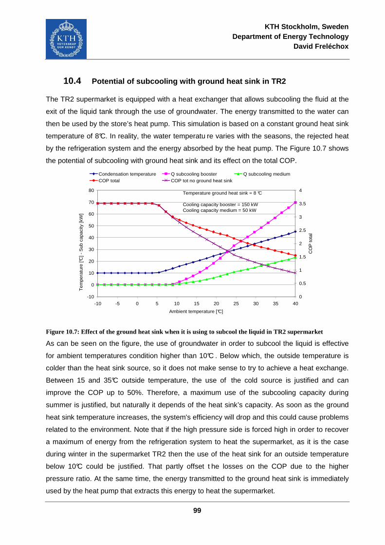
KTH Stockholm, Sweden Department of Energy Technology
David Freléchox
99
10.4 Potential of subcooling with ground heat sink in TR 2
The TR2 supermarket is equipped with a heat exchanger that allows subcooling the fluid at the
exit of the liquid tank through the use of groundwater. The energy transmitted to the water can
then be used by the store’s heat pump. This simulation is based on a constant ground heat sink
temperature of 8°C. In reality, the water temperatu re varies with the seasons, the rejected heat
by the refrigeration system and the energy absorbed by the heat pump. The Figure 10.7 shows
the potential of subcooling with ground heat sink and its effect on the total COP.
-10
0
10
20
30
40
50
60
70
80
-10 -5 0 5 10 15 20 25 30 35 40
Ambient temperature [°C]
Tem
pera
ture
[°C
] - S
ub c
apac
ity [k
W]
0
0.5
1
1.5
2
2.5
3
3.5
4
CO
P to
tal
Condensation temperature Q subcooling booster Q subcooling mediumCOP total COP tot no ground heat sink
Temperature ground heat sink = 8 °C
Cooling capacity booster = 150 kWCooling capacity medium = 50 kW
Figure 10.7: Effect of the ground heat sink when it is using to subcool the liquid in TR2 supermarket
As can be seen on the figure, the use of groundwater in order to subcool the liquid is effective
for ambient temperatures condition higher than 10°C . Below which, the outside temperature is
colder than the heat sink source, so it does not make sense to try to achieve a heat exchange.
Between 15 and 35°C outside temperature, the use of the cold source is justified and can
improve the COP up to 50%. Therefore, a maximum use of the subcooling capacity during
summer is justified, but naturally it depends of the heat sink’s capacity. As soon as the ground
heat sink temperature increases, the system's efficiency will drop and this could cause problems
related to the environment. Note that if the high pressure side is forced high in order to recover
a maximum of energy from the refrigeration system to heat the supermarket, as it is the case
during winter in the supermarket TR2 then the use of the heat sink for an outside temperature
below 10°C could be justified. That partly offset t he losses on the COP due to the higher
pressure ratio. At the same time, the energy transmitted to the ground heat sink is immediately
used by the heat pump that extracts this energy to heat the supermarket.
KTH Stockholm, Sweden Department of Energy Technology
David Freléchox
100
11 Discussion
This study reveals some important points and provides opportunities to continuously improve
the efficiency of refrigeration systems. The focus was set on the natural fluid CO2 which limits
drastically the direct contribution of refrigeration to the greenhouse effect. Its GWP is also the
base unit of measure and equal to 1. It reduces the impact on environment by a factor of
several thousand comparing with other traditional fluids.
Mainly due to its high pressure, CO2 presented a new challenge to the market players in
refrigeration and air conditioning. Most of the components must be improved or completely re-
developed. This process is being carried out by the main manufacturers. Compressors and
most of the valves were well adjusted to fit the use of CO2; however, improvements on cabinet
evaporators and gas coolers are still needed. One of the main problems of the CO2 technology
currently applied in supermarkets is the use of evaporators poorly adapted to this new fluid.
Indeed, tubes diameters and the layout of the evaporator is the same as those used with
traditional fluids. Thus, in order to create enough pressure drops in the evaporator, the
manufacturers voluntarily extend the circuit of the evaporator with a serial connection. Certainly
if smaller and more appropriate tubes were used, a traditional configuration using series /
parallel combinations would provide a better utilization of the exchange surface, or even raise
the temperature of evaporation, which has a direct effect on the energy efficiency. On the other
hand, refined design evaporators would certainly match the internal superheat used with
traditional fluids. Thus, the observed values on CO2 systems around 12 K could be reduced to
7 K. 7 K is a standard value for R404A systems and has been observed in at least one of the
R404A installation at the IWMAC interface.
Field measurements on three supermarkets have been carried out. Two supermarket use CO2
in a transcritical mode and one with a cascade R404A/CO2. The comparison show the highest
COP of about 4.5 on the medium temperature unit and 1.6 on the low temperature unit for the
supermarket using CO2 transcritical TR1. This is mainly du to the use of floating condensation
on this system which is an important advantage to the others. Therefore, the use of the floating
condensation is almost mandatory in the implementation of the fluid in order to achieve high
efficiency. The current limit for condensation temperature is set at 10°C, which should be further
lowered to improve the benefit of CO2 compared to traditional fluids in cold regions. CO2 take
advantage of its high working pressure, the pressure drop across the expansion valve is still
higher than with R404A as example and it allow reducing the condensation temperature
furthermore.
KTH Stockholm, Sweden Department of Energy Technology
David Freléchox
101
However, several installations combine cooling systems with the heating system of the store.
This creates conflicts between the optimization of refrigeration COP and the maximization of
heat recovery. At least two of the facilities investigated in this thesis increase the condensing
temperature to recover more heat during winter. TR2 system raises its high pressure and uses
a borehole to subcool the liquid and avoid the COP losses. Note that the borehole was also
connected to the heat pump of the store. The second system CC1 keep its high pressure at a
high level during the whole year. We have not the possibility to calculate the capacity which is
recovered, so it is difficult to comment on this. As shown in this study, the negative impact of
condensation temperature rise is clearly more pronounced for CO2 systems.
Free heat sink sources as a borehole are particularly favourable in case of carbon dioxide.
Indeed, the COP of a CO2 installation is quite sensitive to subcooling. One Kelvin subcooling
could easily result in 2 times higher effect on COP in the case of CO2 than with R404A. This is
primarily applicable to condensing temperature near the critical point. Thus, the subcooling
potential of a borehole should mainly be used in summer.
Simulations were used in order to unify the working conditions for each supermarket and thus
allow fair comparison between the three systems. Firstly, the simulations were validating with
field measurement. Several comparisons have been carried out. It particularly shows the
influence of the coolant loop on the efficiency. On the function COP versus condensation
temperature, TR1 and TR2 systems have the better COP until the crossover at 25°C
condensation temperature when the cascade system CC1 has the highest COP. When the
influence of the coolant loop is inserted on the plot COP versus outside temperature, then the
TR1 system without coolant loop has the highest COP until 23°C outside temperature. This
transition of the highest COP between transcritical system and cascade system result from a
simulation and in reality the good heat transfer capacities of CO2 could favour it furthermore.
KTH Stockholm, Sweden Department of Energy Technology
David Freléchox
102
Using this simulation and the outside temperature of three different climates which are
Stockholm, Frankfurt and Phoenix an annual simulation has been done. In most countries of
Western Europe the technology of transcritical carbon dioxide is more appropriate than cascade
system R404A/CO2 and reduces the energy consumption of refrigeration systems of about 15 –
20 %. In warmer climate, with temperatures averaging around 20°C, the carbon dioxide in
transcritical mode is less suitable. For very hot climates such as Phoenix/USA, the
overconsumption of a CO2 transcritical installation compared to a cascade system is about
20%. Thus, the elimination of synthetic fluids for this type of climate needs still to be analysed.
The TEWI analysis should be done then to investigate which system has less effect at the
environment. In this analysis the direct and indirect impact are included. Otherwise, an efficient
environmentally friendly replacement for the R404A could be ammonia in a cascade system
with CO2. Elimination may not be the best way; however, limitations on the amount of R404A
used would favour certain environmentally friendly solutions.
Our study also demonstrated some improvements possibilities on CO2 transcritical systems.
Particularly, the importance of the transition temperature applied in the regulation of the
condensation level. A transition temperature at 28°C instead of 31°C will help avoiding increase
in the enthalpy at the evaporator inlet and thus may lead under certain conditions to a 7%
increase of the COP. Another possibility is to desuperheat the fluid at the outlet of the first stage
on a two stage compressor. This leads to a gain up to 7% of the COP. The use of bigger and
high efficient evaporator leads also to a COP improvement of 12 % due to an increase of 5 K
evaporation temperature from -10 to -5°C.
At a practical level, a modification has come to our attention in a positive way. Installing a
frequency converter on compressors, which allow a better control of the system and give
easiest way to fix the evaporation temperature, has lead to a reduction of about 10 % of the
electrical power consumption on medium temperature systems. This is due to the settings
changes and better stability of the evaporating temperature which has led to a few kelvins
reduction of the approach temperature difference. Stable operating conditions give the
possibility to improve most of the settings and adjusting the speed of the compressors at the
request load fits with the optimization process.
KTH Stockholm, Sweden Department of Energy Technology
David Freléchox
103
12 Conclusions and suggestions for future Works
This thesis evaluated different field installations with different refrigeration system solutions.
Computer simulation models for each of the systems under investigation have been run. The
systems under investigation have been compared based on the results from the field
measurements and the computer simulation models. This work compares three different field
installations and shows the difficulties to make comparison on the base of field measurement.
Various different parameters such as the load ratio, the use of a borehole, the heat recovery
requirements or the heat recovery system influence the COP of the system and thus make the
comparison difficult.
This study demonstrated using our simulation models and according to the field measurements
that at low condensing temperatures the CO2 transcritical system reach the highest COP and at
high condensing temperatures the cascade R404A/CO2 system is more efficient. The crossover
on the COP between these two solutions is floating between 15 and 27°C depending on the
absence of a coolant loop, or the use of free desuperheating between two compression stages,
or is influenced by the heat exchange proprieties of the fluid.
In addition, the floating condensation and lowering the condensing temperature limit allows a
significant increase in the COP. On a transcritical system, the use of floating condensation up to
10°C allow reaching a total COP of 3.7 with a load ratio of 3.
In the near future and within this project, other installations will be analyzed and simulated
following the same procedure as adapted in this thesis. Specifically, one more cascade system
with variable speed pumps and a supermarkets using CO2 pump circulation technology. Also
analysis of supermarkets using traditional technologies with only synthetic fluids, especially
R404A is underway. This will allow comparison of all systems, new and old technologies,
natural and synthetic refrigerants.
The experimental and theoretical studies reported in this thesis prove that CO2 based system
solutions investigated can be efficient solutions for supermarket refrigeration; however,
comparison with traditional systems is needed and will be presented in following publications in
the ongoing project.
Freléchox David Stockholm
13 August 2009
KTH Stockholm, Sweden Department of Energy Technology
David Freléchox
104
13 References
[ANT09] Antonsson M. (2009): Green and Cool AB, Personnal contact, Email from 1st June
2009. Available at : www.greenandcoolco2.com [ARI05] Arias J. (2005): Energy Usage in Supermarkets – Modelling and Field
Measurements, Doctoral Thesis in Energy Technology, KTH Stockholm. [BIT09] Bitzer (2009): Bitzer Software 5.1.2, available at http://www.bitzer.de/eng/documentation/list/software. [BIV04] Bivens D., Gage C. (2004): Commercial Refrigeration System Emissions. The Earth
Technologies Forum, Washington D.C. [CHE05] Chen Y., Gu j. (2005): The optimum high pressure for CO2 Transcritical
Refrigeration Systems with Internal Heat Exchangers, International Journal of Refrigeration 28, p. 1238-1249.
[DAB82] Dabiri A. E., Rice C. K. (1982): A compressor simulation model with corrections fort
he level of suction gas superheat, ASHRAE Transactions, Vol. 87, Part 2, p. 771-782.
[DAN06] Danfoss Refrigeration (2006): Danfoss Motorized Valves type ICM – Motor Actuators
type ICAD, Technical leaflet 02-2006. [DOR09] Dorin (2009), “The widest CO2 compressor range, carbon dioxide for all your
needs”, available at: www.dorin.com/documents/Download/19/CO2_-0809a.pdf, product information sheet
[EPT09] EPTA GmbH, Kröger J. (2009): Weltneuheit „Zero°“: Konstante
Verdampfungstemperatur von 0°C – Energieersparnis v on bis zu 20 Prozent, KI Kälte-Luft-Klimatechnik, Mai 2009.
[KIM03] Kim M-H, Pettersen J., Bullard C.W.(2004): Fundamental process and system
design issues in CO2 vapor compresion systems, Progress in Energy and Combustion Science 30, p.119-174 (122,
[GEY09] Ge Y.T., Tassou S.A. (2009): Control optimisation of CO2 cycles for medium
temperature retail food refrigeration systems, International Journal of Refrigeration, 2009. (not already published , in press).
[GIR04] Girotto S., Minetto S.,Nekska P.(2004): Commercial refrigeration system using CO2
as the refrigerant, International Journal of Refrigeration 27, p. 717-723. [GIR05] Girotto S. (2005): Commercial and industrial refrigeration, Application of carbon
dioxide as a secondary fluid with phase change, in the low temperature cycle of cascade systems and direct expansion systems with transfer of heat into the environment, XI European conference Politecnico of Milano, On technological innovations in air conditioning and refrigeration, June 2005.
KTH Stockholm, Sweden Department of Energy Technology
David Freléchox
105
[GRA05] Granryd E. and all. (2005): Refrigerating Engineering, Departement of Energy
Technology, Division of Applied Thermodynamics and Refrigeration, Royal Institute of Technology, KTH, Stockholm 2005.
[GRA07] Granryd E. (2007): Optimum flow rates in indirect systems. International Congress of
Refrigeration, Beijing 2007. [GRO08] Groll E. A., Garimella S. V. (2008): Experimental evaluation of a miniature rotary
compressor for application in electronics cooling, International Compressor Engineering Conference at Purdue, 14-17 July 2008, 1115 p.2-3.
[HAA05] Haaf S., Heinbokel B., Gernemann A.: First CO2 Refrigeration System for Medium-
and Low- Temperature Refrgeration at Swiss Megastore, Linde Kaeltetechnik News 02 / 2005.
[HIN09] Hinde D., Shitong Z., Lin L. (2009): Carbon dioxide in North American Supermarket.
ASHRAE Journal, Vol. 51, No 2, February 2009, p. 18-24. [INC96] Incropera F., DeWitt D. (1996): Fundamentals of Heat and Mass Transfer 4th Edition,
John Wiley & Sons, p 284-332 and 535 – 569. [IWM09] Iwmac (2009), “Centralised operation and surveillance, by use of WEB technology”,
available at: http://www.iwmac.no/english/ [JOH09] Johansson S. (2009), Master Thesis “Evaluation of CO2 supermarket refrigeration
systems”, KTH Stockholm 2009. [KLE06] Klein S. A. (2006), Engineering Equations Solver (EES), Madison, USA: F-Chart
Software [PAL04] Palandre L., Clodic D., Kuijpers L. (2004) : HCFCs and HFCs emissions from the
refrigerating systems for the period 2004 – 2015. The Earth Technologies Forum, Washington D.C.
[RDM09] RDM (2009), “Centralised operation and surveillance, access through modem line”,
available at: http://www.resourcedm.com/ [REM01] Remund J., Lang R., Kunz S. (2001), Meteonorm (version 4.10), Bern: Meteotest [SAW08] Sawalha S. (2008): Carbon Dioxide in Supermarket Refrigeration, Doctoral Thesis in
Energy Technology, KTH Stockholm, p.51, 49, [SAW09] Sawalha S. (2009): Presentation CO2 and transcritical cycle, lecture on 03.03.2009,
KTH Stockholm [SVE09] Sveriges meteorologiska och hydrologiska Institut (2009): Available at : www.smhi.se [VIK09] Viktorsson L. (2009): Partor AB, Personnal contact, Email from 4th June 2009.
Available at : www.partor.se
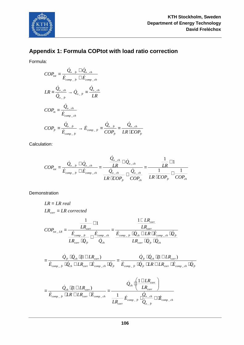
KTH Stockholm, Sweden Department of Energy Technology
David Freléchox
106
Appendix 1: Formula COPtot with load ratio correcti on
Formula:
chcompfrcomp
chofrotot EE
QQCOP
__
__
&&
&&
++
=
LR
Q
QLR cho
frofro
cho __
_
_&
&&
&
=→=
chcomp
chom E
QCOP
_
_
&
&
=
fr
cho
fr
frofrcomp
frcomp
frofr COPLR
Q
COP
QE
E
QCOP
⋅==→= __
__
_&&
&&
&
Calculation:
chfrch
cho
fr
cho
chocho
chcompfrcomp
chofrotot
COPCOPLR
LR
COP
Q
COPLR
Q
QLR
Q
EE
QQCOP
11
11
__
__
__
__
+⋅
+=
+⋅
+=
++
=&&
&&
&&
&&
Demonstration
correctedLRLR
realLRLR
corr ==
chcompfro
chofrcomp
corr
corr
corrch
chcompcorrfrcomp
corrch
frchcompcorrfrfrcomp
corrchfr
frchcompcorrchfrcomp
corrchfr
chfrcorr
frchcompchfrcomp
corr
corr
ch
chcomp
frcorr
frcomp
corrLRtot
EQ
QE
LR
LR
LRQ
ELRLRE
LRQ
QELRLRQE
LRQQ
QELRQE
LRQQ
QQLR
QELRQELR
LR
Q
E
QLR
ELR
COP
__
__
__
____
_____
1
1
)1(
)1()1(
11
1
&&
&&
&
&&
&
&&&&
&&
&&&&
&&
&&
&&&&
&
&
&
&
⋅+⋅
+⋅=
⋅+⋅+⋅=
⋅⋅+⋅⋅+⋅⋅
=⋅⋅+⋅
+⋅⋅=
⋅⋅⋅⋅+⋅
+
=+
⋅
+=