Managerial EpidemiologyPart II

Ty Borders, Ph.D.

Assistant Professor

Department of Health Services Research & Management

School of Medicine

Objectives

• Identify groups at higher risk for poor health and need for health service– Calculate Relative Risk, Attributable Risk, & Odds Ratio

• Discuss strengths and weaknesses of designs to identify at risk groups– Case control studies

– Prospective and retrospective cohort studies

Epidemiology and Levels of Disease Prevention

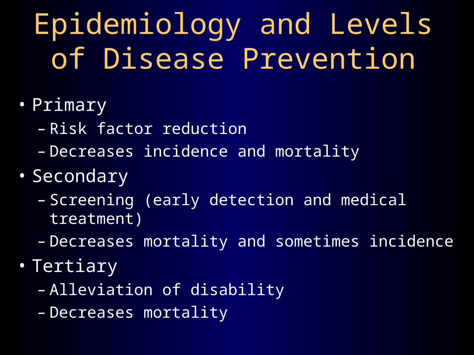
• Primary– Risk factor reduction– Decreases incidence and mortality

• Secondary– Screening (early detection and medical

treatment)– Decreases mortality and sometimes incidence

• Tertiary– Alleviation of disability– Decreases mortality

Identifying High Risk Groups: Observational Studies

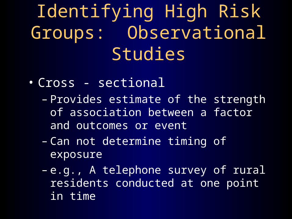
• Cross - sectional– Provides estimate of the strength of association

between a factor and outcomes or event– Can not determine timing of exposure– e.g., A telephone survey of rural residents

conducted at one point in time

Observational Studies (cont.)

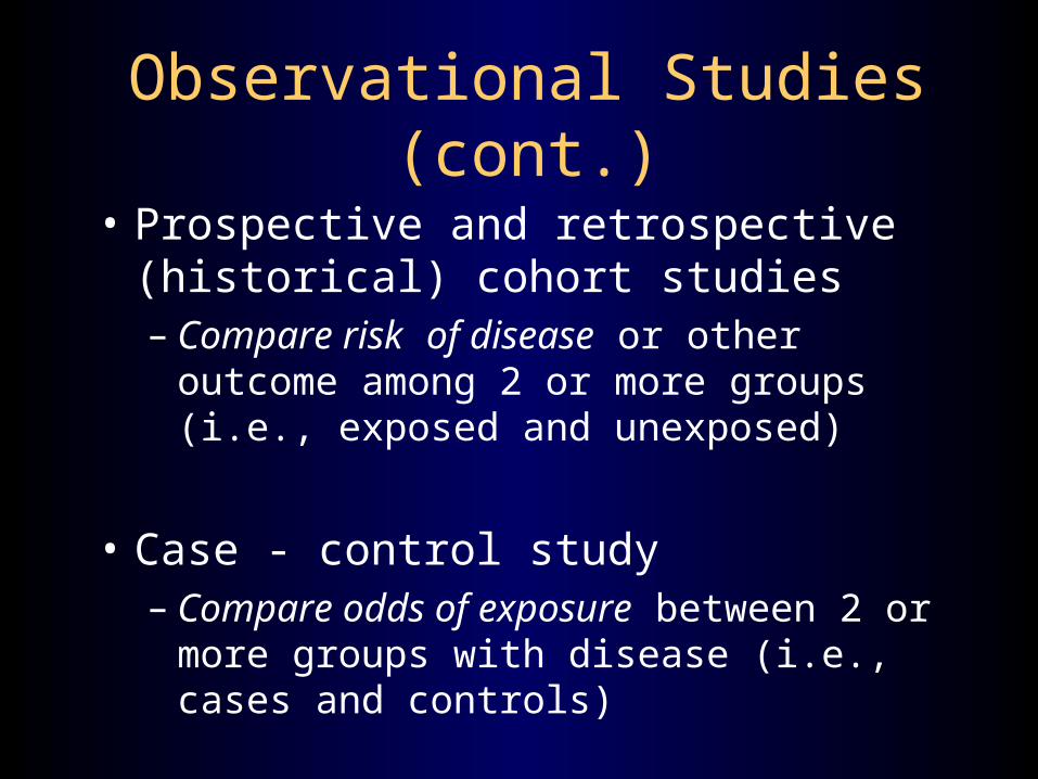
• Prospective and retrospective (historical) cohort studies– Compare risk of disease or other outcome

among 2 or more groups (i.e., exposed and unexposed)

• Case - control study– Compare odds of exposure between 2 or more

groups with disease (i.e., cases and controls)

Risk Factors

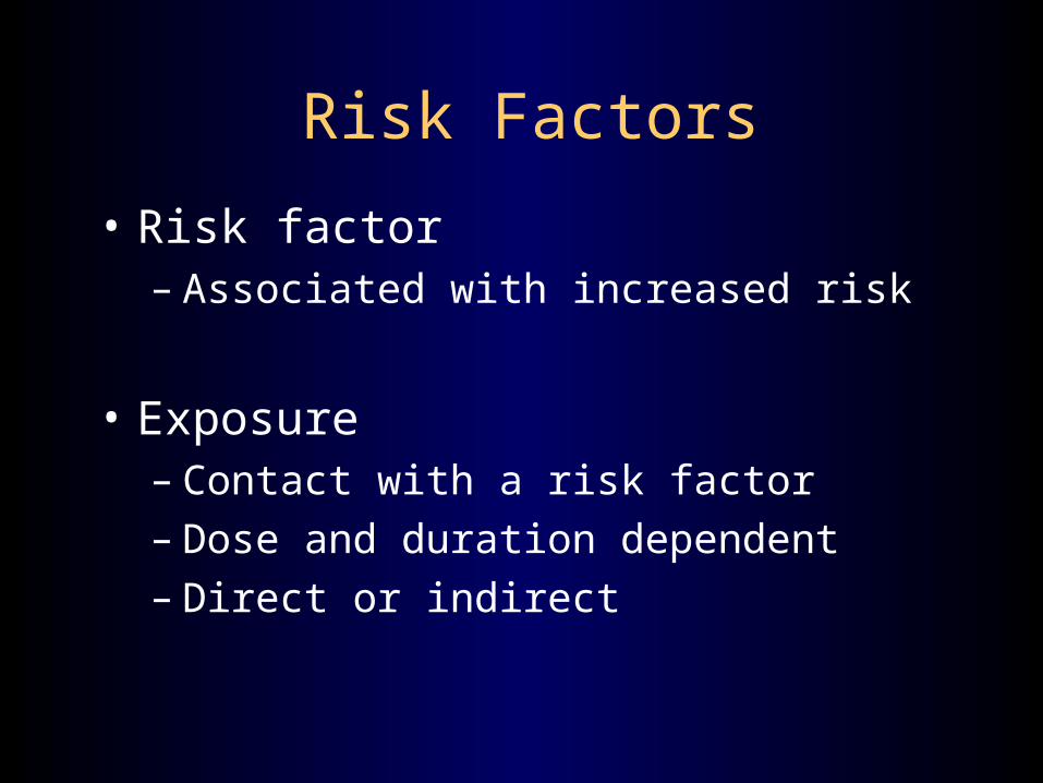
• Risk factor– Associated with increased risk

• Exposure– Contact with a risk factor– Dose and duration dependent– Direct or indirect

Cohort Studies

Onset of study

Time

Exposed

Unexposed

Eligible subjects Disease

No Disease

Disease

No Disease

Direction of inquiry

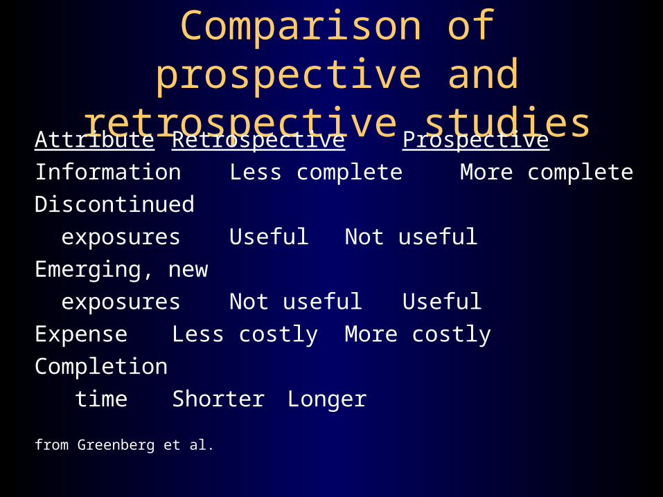
Comparison of prospective and retrospective studies

Attribute Retrospective Prospective

Information Less complete More complete

Discontinued

exposures Useful Not useful

Emerging, new

exposures Not useful Useful

Expense Less costly More costly

Completion

time Shorter Longer

from Greenberg et al.

Adv./Disadv. of cohort studiesAdvantages Disadvantages

Direct calculation Time consuming

of relative risk

May yield info. on incidence Require large sample sizes

Clear temporal relationship Expensive

Can yield info. on multiple Not efficient for study of

exposures rare events

Minimizes bias Losses to follow-up

Strongest observational design

for establishing cause-effect

from Greenberg et al.

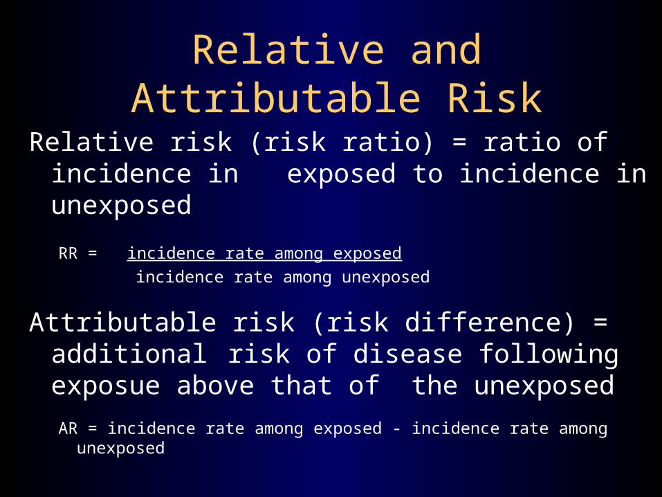
Relative and Attributable Risk

Relative risk (risk ratio) = ratio of incidence in exposed to incidence in unexposed

RR = incidence rate among exposed

incidence rate among unexposed

Attributable risk (risk difference) = additional risk of disease following exposue above that of the unexposed

AR = incidence rate among exposed - incidence rate among unexposed

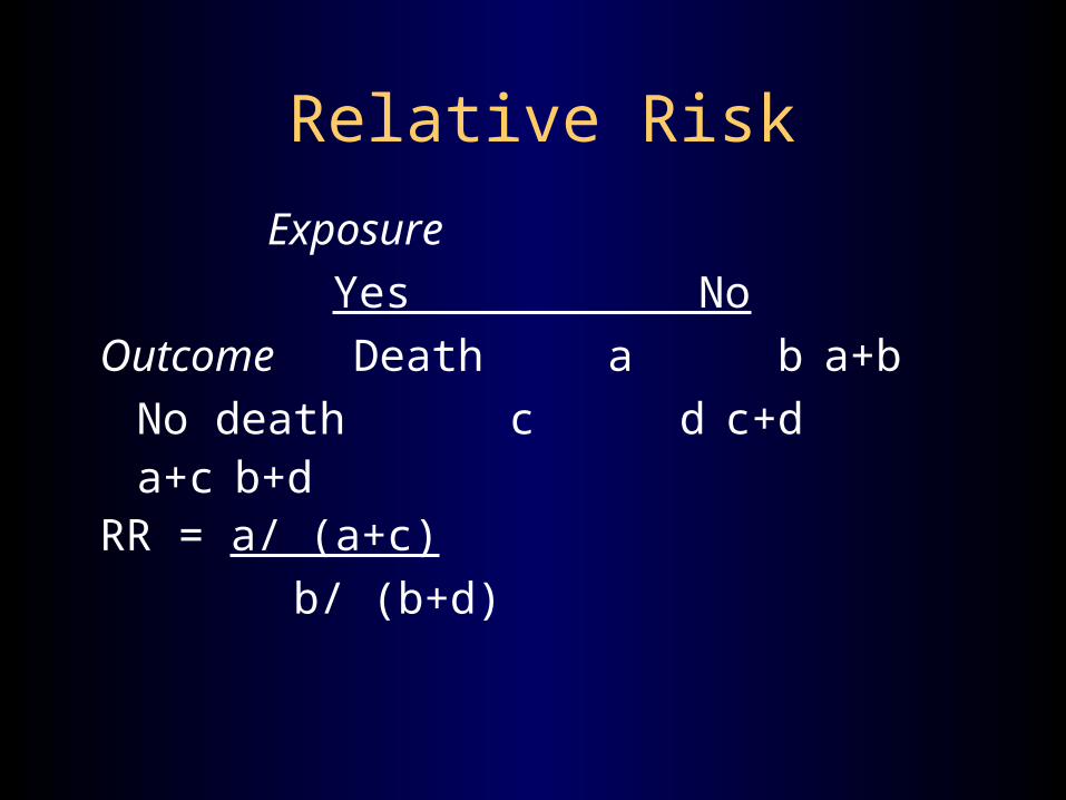
Relative Risk

Exposure

Yes No

Outcome Death a b a+b

No death c d c+da+c b+d

RR = a/ (a+c)

b/ (b+d)

Example of Relative Risk

Apgar score 0-3 4-6

Outcome Death 42 43 85No death 80 302 382

122 345 467

Risk among exposed = 42 / 122 = 34.4%Risk among unexposed = 43 / 345 = 12.5%RR = 34.4 / 12.5 = 2.8

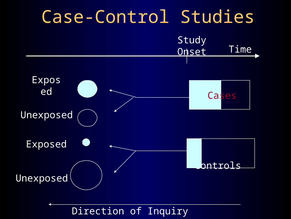
Case-Control Studies

Time

Controls

Direction of Inquiry

CasesExposed

Unexposed

Unexposed

Exposed

Study Onset

Cases and controls

• Cases– Identified and selected from a defined source

population (e.g., all patients from a clinic, hospital, HMO, state, or nation)

– Likelihood of a case being included in study must not depend on exposure to risk factor

– Criteria for defining cases should be sensitive and specific

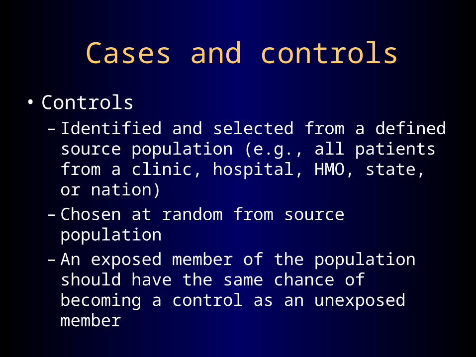
Cases and controls

• Controls– Identified and selected from a defined source

population (e.g., all patients from a clinic, hospital, HMO, state, or nation)

– Chosen at random from source population– An exposed member of the population should have

the same chance of becoming a control as an unexposed member

Exposure status

• Interviews and questionnaires typically used

• Objective measures preferred– e.g., biological markers, such as a measure of an

agent in the blood– Not always feasible, especially if test is invasive– Many exposures don’t have biological markers– Biological marker may not be present when test is

taken (e.g., aspirin quickly metabolized)

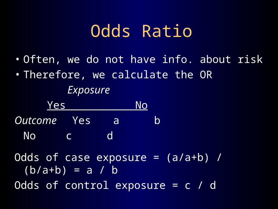
Odds Ratio

• Often, we do not have info. about risk

• Therefore, we calculate the OR

Exposure

Yes No

Outcome Yes a b

No c d

Odds of case exposure = (a/a+b) / (b/a+b) = a / b

Odds of control exposure = c / d

Example of Odds Ratio

Exposure

Yes No

Cases 50 15

Controls 30 20

OR = (a/b) / (c/d)

= ad / bc = 50*20 / 30*15 = 2.22

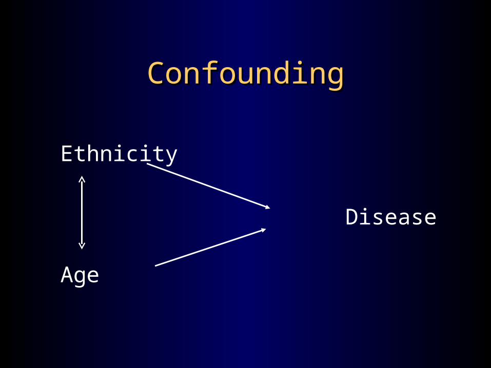
ConfoundingConfounding

Ethnicity

Disease

Age

ConfoundingConfoundingAge distribution (%)

44.0

51.6

36.1

38.0

38.3

38.2

24.6

26.7

25.7

27.0

24.1

25.7

16.8

16.2

19.6

19.1

19.3

19.2

14.7

5.6

18.6

15.9

18.4

16.9

Other Races

Hispanics

Non-Hispanic Whites

Urban residents

Rural residents

Overall

81+

76-80

71-75

65-70

ConfoundingConfoundingAge distribution (%)

44.0

51.6

36.1

38.0

38.3

38.2

24.6

26.7

25.7

27.0

24.1

25.7

16.8

16.2

19.6

19.1

19.3

19.2

14.7

5.6

18.6

15.9

18.4

16.9

Other Races

Hispanics

Non-Hispanic Whites

Urban residents

Rural residents

Overall

81+

76-80

71-75

65-70

1.39

0.91

0.74

0.72

0.68

0.71

2.18

0.61

0.53

0.57

0.59

0.83

-0.5 0.5 1.5 2.5

Hypertension

CHD

Lung disease

Stroke

Arthritis

Diabetes

OR

Adj. OR

Odds of DiseaseHispanics Relative to Non-Hispanic Whites

Adjusted and unadjusted

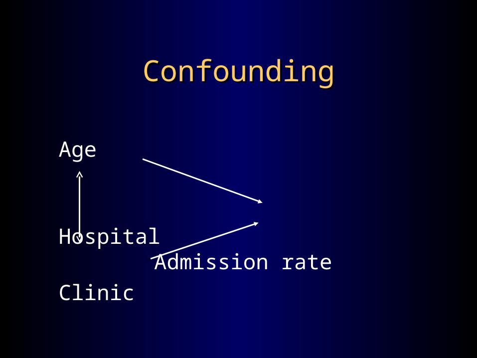
ConfoundingConfounding

Age

Hospital

Admission rate

Clinic

StandardizationStandardization

• Direct– Derived by applying category-specific rates

observed in each study population to a standard population

– Choice of study population• One of the populations to be compared

• Study populations combined

• An outside standard of interests (e.g., 1960 U.S. population)

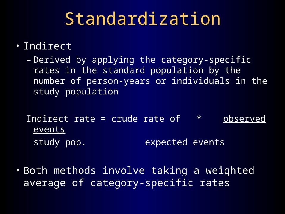
StandardizationStandardization

• Indirect– Derived by applying the category-specific rates in the

standard population by the number of person-years or individuals in the study population

Indirect rate = crude rate of * observed events

study pop. expected events

• Both methods involve taking a weighted average of category-specific rates

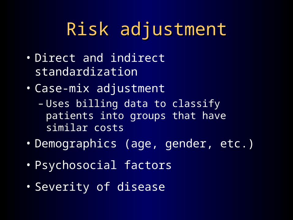
Risk adjustmentRisk adjustment

• Direct and indirect standardization

• Case-mix adjustment– Uses billing data to classify patients into groups

that have similar costs

• Demographics (age, gender, etc.)

• Psychosocial factors

• Severity of disease

Survey Research Example

• Purpose– To determine who migrates or travels for physician care

– To determine why they migrate or travel for physician care

• Dependent variable– Whether the physician was located in the individual’s

home county (local market area) or another county (external market area)

Research MethodologyResearch Methodology

• Cross-sectional, population-based survey of– Perceived health status (e.g. SF-12)

– Health behaviors

– Realized health care utilization

– Accessibility of local providers

– Satisfaction with care

– Demographic factors

– Economic factors, including health insurance coverage

– Health services use

Independent Variables Independent Variables Health system factorsHealth system factors

• Perceived shortage of local family physicians – note: dummy variables created for most independent

variables

• Perceived shortage of local specialty physicians

• Rating of local delivery system– (excellent/very good versus good/fair/poor)

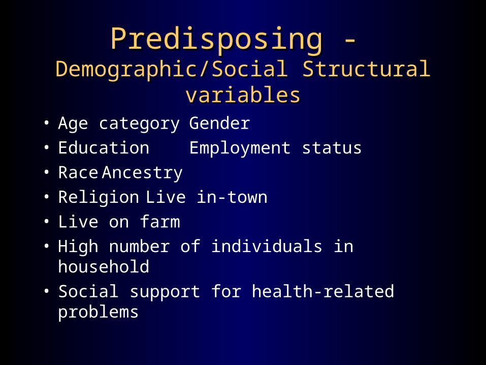
Predisposing - Predisposing - Demographic/Social Structural variablesDemographic/Social Structural variables

• Age category Gender• Education Employment status • Race Ancestry• Religion Live in-town• Live on farm• High number of individuals in household• Social support for health-related problems

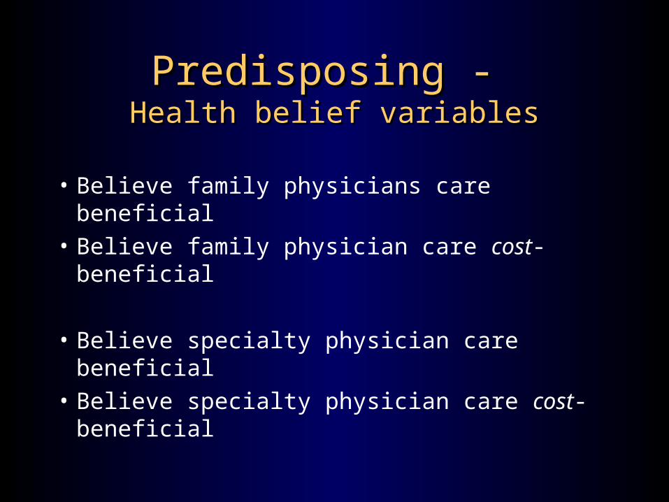
Predisposing - Predisposing - Health belief variablesHealth belief variables

• Believe family physicians care beneficial

• Believe family physician care cost-beneficial

• Believe specialty physician care beneficial

• Believe specialty physician care cost-beneficial

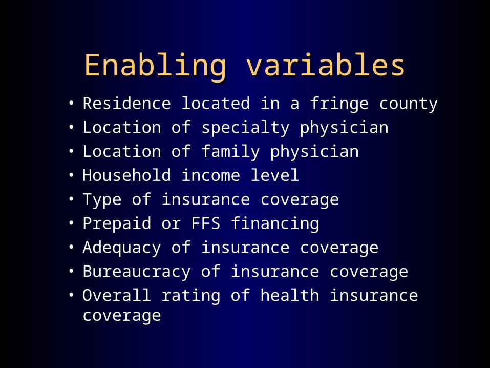
Enabling variablesEnabling variables• Residence located in a fringe county• Location of specialty physician • Location of family physician• Household income level• Type of insurance coverage• Prepaid or FFS financing• Adequacy of insurance coverage• Bureaucracy of insurance coverage• Overall rating of health insurance coverage

Need variablesNeed variables

• Modified SF-12 Physical Component Score

• Modified SF-12 Mental Component Score

• High, moderate, or low user of physician services

Family Physician Migration -Significant Odds Ratios

0.306

2.278

0.47 0.489

2.919

0.375

0

0.5

1

1.5

2

2.5

3P

os

.ra

tin

g

Fa

m.

sh

ort

ag

e

Lu

the

ran

Liv

e in

-to

wn

Sp

ec

. o

ut

of

co

un

ty

Pri

va

tein

s.

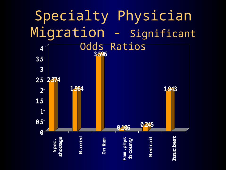
Specialty Physician Migration - Significant Odds Ratios

2.3741.964

3.596

0.106 0.245

1.943

0

0.5

1

1.5

2

2.5

3

3.5

4S

pec.

shor

tage

Mar

ried

On

farm

Fam

. phy

sin

cou

nty

Med

icai

d

Insu

r. b

est

Market Research ImplicationsMarket Research Implications

• Supply of rural physicians and health system quality– Health systems linkages– Hospital/health system ownership– Telemedicine

• Physicians needs among market segments– Target groups of migrators

(e.g. farmers, married people)

Another example: Another example: Underservice among malesUnderservice among males

• Cross-sectional survey conducted in a rural Iowa county

• Separate analyses for males and females

• Identified risk factors associated with service use to segment the market

Segmented by marital statusSegmented by marital status

0.992 0.941

2.31

1.268 1.29

3.544

0

0.5

1

1.5

2

2.5

3

3.5

4

4.5

5

Adjusted Log Log No. of visits

Single Married

Segmented by employmentSegmented by employment

1.405 1.469

4.588

1.068 1.033

2.413

0

0.5

1

1.5

2

2.5

3

3.5

4

4.5

5

Adjusted Log Log No. of visits

Unemployed

Employed

Strategies to attract malesStrategies to attract males

• Price (not too important in health care)

• Distribution (e.g. extended office hours)

• Product (e.g. lower office waiting times)

• Promotion