Nonlinear Finite Elements for Continua and Structures, Second Edition. Ted Belytschko, Wing Kam Liu, Brian Moran, and Khalil I. Elkhodary. © 2014 John Wiley & Sons, Ltd. Published 2014 by John Wiley & Sons, Ltd. Companion Website: www.wiley.com/go/belytschko

Introduction

1

1.1 Nonlinear Finite Elements in Design

Nonlinear finite element analysis is an essential component of computer-aided design. Testing of prototypes is increasingly being replaced by simulation with nonlinear finite element methods because this provides a more rapid and less expensive way to evaluate design concepts and design details. For example, in the field of automotive design, simulation of crashes is replacing full-scale tests, for both the evaluation of early design concepts and details of the final design, such as accelerometer placement for airbag deployment, padding of the interior, and selection of materials and component cross-sections for meeting crashworthiness criteria. In many fields of manufacturing, simulation is speeding the design process by allowing simulation of processes such as sheet-metal forming, extrusion, and casting. In the electronics industries, simulation is replacing drop-tests for the evaluation of product durability.

Both analysts and developers of nonlinear finite element programs should understand the fundamental concepts of nonlinear finite element analysis. Without an understanding of the fundamentals, a finite element program is a black box that provides simulations. However, nonlinear finite element analysis confronts the analyst with many choices and pitfalls. Without an understanding of the implication and meaning of these choices and difficulties, an analyst is at a severe disadvantage.

The purpose of this book is to describe the methods of nonlinear finite element analysis for solid mechanics. The intent is to provide an integrated treatment so that the reader can gain an understanding of the fundamental methods, a feeling for the comparative usefulness of different approaches and an appreciation of the difficulties which lurk in the nonlinear world.

0002023647.INDD 1 10/5/2013 11:17:15 AM

COPYRIG

HTED M

ATERIAL

2 Nonlinear Finite Elements for Continua and Structures

At the same time, enough detail about the implementation of various techniques is given so that they can be programmed.

Nonlinear analysis consists of the following steps:

1. Development of a model2. Formulation of the governing equations3. Discretization of the equations4. Solution of the equations5. Interpretation of the results.

Items 2 to 4 typically are within the analysis code, while the analyst is responsible for items 1 and 5.

Model development has changed markedly in the past decade. Until the 1990s, model development emphasized the extraction of the essential elements of mechanical behavior. The objective was to identify the simplest model which could replicate the behavior of interest.

It is now becoming common in industry to develop a single, detailed model of a design and to use it to examine all of the engineering criteria which are of interest. The impetus for this approach to modeling is that it costs far more to make several meshes for an engineering product than can be saved by specializing meshes for each application. For example, the same finite element model of a laptop computer can be used for a drop-test simulation, a linear static analysis and a thermal analysis. By using the same model for all of these analyses, a significant amount of engineering time can be saved. While this approach is not recommended in all situations, it is becoming commonplace in industry.

In the near future the finite element model may become a ‘virtual’ prototype that can be used for checking many aspects of a design’s performance. The decreasing cost of computer time and the increasing speed of computers make this approach highly cost-effective. However, the user of finite element software must still be able to evaluate the suitability of a model for a particular analysis and understand its limitations.

The formulation of the governing equations and their discretization is today largely in the hands of the software developers. However, an analyst who does not understand the funda-mentals of the software faces many perils, because some approaches and software may be unsuitable. Furthermore, to convert experimental data to input, the analyst must be aware of the stress and strain measures used in the program and by the experimentalist who provided material data. The analyst must understand the sensitivity of response to the data and how to assess it. An effective analyst must be aware of the likely sources of error, how to check for these errors and estimate their magnitudes, and the limitations and strengths of various algorithms.

The solution of the discrete equations also presents many choices. An inappropriate choice will result in very long run times which can prevent the analyst from obtaining the results within the time schedule. An understanding of the advantages and disadvantages and the approximate computer times required for various solution procedures is invaluable in the selection of a good strategy for developing a reasonable model and selecting the best solution procedure.

The analyst’s role is most crucial in the interpretation of results. In addition to the approximations inherent even in linear finite element models, nonlinear analyses are often sensitive to many factors that can make a single simulation quite misleading. Nonlinear solids

0002023647.INDD 2 10/5/2013 11:17:15 AM

Introduction 3

can undergo instabilities, their response can be sensitive to imperfections, and the results can depend dramatically on material parameters. Unless the analyst is aware of these phenomena, misinterpretation of simulation results is quite possible.

Despite these pitfalls, our views on the usefulness and potential of nonlinear finite element analyses are very sanguine. In many industries, nonlinear finite element analyses have shor-tened design cycles and dramatically reduced the need for prototype tests. Simulations, because of the wide variety of output they produce and the ease of doing ‘what-ifs,’ can lead to tremendous improvements of the engineer’s understanding of the basic physics of a product’s behavior under various environments. While tests give the gross but important result of whether the product withstands a certain environment, they usually provide little of the detail of the behavior of the product on which a redesign can be based if the product does not meet a test. Computer simulations, on the other hand, give detailed histories of stress and strain and other state variables, which in the hands of a good engineer give valuable insight into how to redesign the product.

Like many finite element books, this book presents a large variety of methods and recipes for the solution of engineering and scientific problems by the finite element method. However, to preserve a pedagogic character, we have interwoven several themes into the book which we feel are of central importance in nonlinear analysis. These include the following:

1. The selection of appropriate methods for the problem at hand2. The selection of a suitable mesh description and kinematic and kinetic descriptions for a

given problem3. The examination of stability of the solution and the solution procedure4. An awareness of the smoothness of the response of the model and its implication on the

quality and difficulty of the solution5. The role of major assumptions and the likely sources of error.

The selection of an appropriate mesh description, i.e. whether a Lagrangian, Eulerian or arbitrary Lagrangian Eulerian mesh is used, is important for many of the large deformation problems encountered in process simulation and failure analysis. The effects of mesh distortion need to be understood, and the advantages of different types of mesh descriptions should be borne in mind in the selection.

Stability is a ubiquitous issue in the simulation of nonlinear processes. In numerical simu-lations, it is possible to obtain solutions which are not physically stable and therefore quite meaningless. Many solutions are sensitive to imperfections of material and load parameters; in some cases, there is even sensitivity to the mesh employed in the solution. A knowledgeable user of nonlinear finite element software must be aware of these characteristics and the associated pitfalls, otherwise the results obtained by elaborate computer simulations can be quite misleading and lead to incorrect design decisions.

The issue of smoothness is also ubiquitous in nonlinear finite element analysis. Lack of smoothness degrades the robustness of most algorithms and can introduce undesirable noise into the solution. Techniques have been developed which improve the smoothness of the response; these are called regularization procedures. However, regularization procedures are often not based on physical phenomena and in many cases the constants associated with the regularization are difficult to determine. Therefore, an analyst is often confronted with the dilemma of whether to choose a method which leads to smoother solutions or to deal with a

0002023647.INDD 3 10/5/2013 11:17:15 AM

4 Nonlinear Finite Elements for Continua and Structures

discontinuous response. An understanding of the effects of regularization parameters and of the presence of hidden regularizations, such as penalty methods in contact-impact, and an appreciation of the benefits of these methods, is highly desirable.

The accuracy and stability of solutions are important issues in nonlinear analysis. These issues manifest themselves in many ways. For example, in the selection of an element, the analyst must be aware of stability and locking characteristics of various elements. A judicious selection of an element involves factors such as the stability of the element for the problem at hand, the expected smoothness of the solution and the magnitude of deformations expected. In addition, the analyst must be aware of the complexity of nonlinear solutions. The possibility of both physical and numerical instabilities must be kept in mind and checked in a solution.

Thus the informed use of nonlinear software in both industry and research requires consid-erable understanding of nonlinear finite element methods. It is the objective of this book to provide this understanding and to make the reader aware of the many interesting challenges and opportunities in nonlinear finite element analysis.

1.2 Related Books and a Brief History of Nonlinear Finite Elements

Several excellent texts and monographs devoted either entirely or partially to nonlinear finite element analysis have already been published. Books dealing only with nonlinear finite element analysis include Oden (1972), Crisfield (1991), Kleiber (1989), and Zhong (1993). Oden’s work is particularly noteworthy since it pioneered the field of nonlinear finite element analysis of solids and structures. Recent books are Simo and Hughes (1998) and Bonet and Wood (1997). Some of the books which are partially devoted to nonlinear analysis are Belytschko and Hughes (1983), Zienkiewicz and Taylor (1991), Bathe (1996) and Cook, Malkus and Plesha (1989). These books provide useful introductions to nonlinear finite element analysis. As a companion book, a treatment of linear finite element analysis is also useful. The most comprehensive are Hughes (1987) and Zienkiewicz and Taylor (1991).

In the following, we recount a brief history of nonlinear finite element methods. This account differs somewhat from those in many other books in that it focuses more on the software than published works. In nonlinear finite element analysis, as in many endeavors in this information-computer age, the software often represents a better guide to the state-of-the-art than the literature.

Nonlinear finite element methods have many roots. Not long after the linear finite element method became known through the work of the Boeing group and the famous paper of Turner, et al. (1956), engineers in many universities and research laboratories began extensions of the method to nonlinear, small-displacement static problems. It is difficult to convey the excitement of the early finite element community and the disdain of classical researchers for the method. For example, for many years the Journal of Applied Mechanics shunned papers on the finite element method because it was considered of no scientific substance. But to many, particularly engineers who had to deal with engineering problems, the promise of the finite element method was clear: it offered the possibility of dealing with the complex shapes of real designs.

The excitement in the 1960s was fueled by Ed Wilson’s liberal distribution of his first pro-grams. The first generation of these programs had no name. In many laboratories throughout the world, engineers developed new applications by modifying and extending these early

0002023647.INDD 4 10/5/2013 11:17:15 AM

Introduction 5

codes developed at Berkeley; they had a tremendous impact on engineering and the subsequent development of finite element software. The second generation of linear programs developed at Berkeley were called SAP (Structural Analysis Program). The first nonlinear program which evolved from this work at Berkeley was NONSAP, which had capabilities for equilibrium solutions and the solution of transient problems by implicit integration.

Among the first papers on nonlinear finite element methods were Argyris (1965) and Marcal and King (1967). The number of papers soon proliferated, and software soon followed. Pedro Marcal taught at Brown University for a time, but he set up a firm to market the first nonlinear commercial finite element program in 1969; the program was called MARC and it is still a major player. At about the same time, John Swanson was developing a nonlinear finite element program at Westinghouse for nuclear applications. He left Westinghouse in 1969 to market the program ANSYS, which for many years dominated the commercial nonlinear finite element scene, although it focused more on nonlinear materials than the complete nonlinear problem.

Two other major players in the early commercial software scene were David Hibbitt and Klaus-Jürgen Bathe. Hibbitt worked with Pedro Marcal until 1972, and then co-founded HKS, which markets ABAQUS. This program has had substantial impact because it was one of the first finite element programs to introduce gateways for researchers to add elements and material models. Jürgen Bathe launched his program shortly after obtaining his PhD at Berkeley under the tutelage of Ed Wilson when he began teaching at MIT. It was an outgrowth of the NONSAP codes, and was called ADINA.

The commercial finite element programs marketed until about 1990 focused on static solu-tions and dynamic solutions by implicit methods. There were terrific advances in these methods in the 1970s, generated mainly by the Berkeley researchers and those with Berkeley roots: Thomas JR Hughes, Robert Taylor, Juan Simo, Jürgen Bathe, Carlos Felippa, Pal Bergan, Kaspar Willam, Ekerhard Ramm and Michael Ortiz are some of the prominent researchers who have been at Berkeley; it was undoubtedly the main incubator in the early years of finite elements.

Another lineage of modern nonlinear software is the explicit finite element codes. Explicit finite element methods in their early years were strongly influenced by the work in the DOE laboratories, particularly the so-called hydro-codes, Wilkins (1964).

In 1964, Costantino developed what was probably the first explicit finite element program, at the IIT Research Institute in Chicago (Costantino, 1967). It was limited to linear materials and small deformations, and computed the internal nodal forces by multiplying a banded form of the stiffness matrix by the nodal displacements. It was first run on an IBM 7040 series com-puter, which cost millions of dollars and had a speed of far less than 1 megaflop (million floating point operations per second) and 32 000 words of RAM. The stiffness matrix was stored on a tape and the progress of a calculation could be gauged by watching the tape drive; after every step, the tape drive would reverse to permit a read of the stiffness matrix. These and the later Control Data machines with similar specifications, the CDC 6400 and 6600, were the machines on which finite element codes were run in the 1960s. A CDC 6400 cost almost $10 million, had 32k words of memory (for storing everything including the operating system and compiler) and a real speed of about one megaflop.

In 1969, in order to sell a proposal to the Air Force, the senior author developed what has come to be known as the element-by-element technique: the computation of the nodal forces without use of a stiffness matrix. The resulting program, SAMSON, was a two-dimensional finite element program which was used for a decade by weapons laboratories in the US. In

0002023647.INDD 5 10/5/2013 11:17:16 AM

6 Nonlinear Finite Elements for Continua and Structures

1972, the program was extended to fully nonlinear three-dimensional transient analysis of structures and called WRECKER. The funding was provided by a visionary program manager, Lee Ovenshire, of the US Department of Transportation, who foresaw in the early 1970s that crash testing of automobiles could be replaced by simulation.

However, it was a little ahead of its time, for at that time a simulation of a 300-element model for a 20 ms simulation took about 30 hours of computer time, which cost about $30 000, the equivalent of three years’ salary of an Assistant Professor. Lee Ovenshire’s program funded several pioneering efforts: Hughes’s work on contact-impact, Ivor McIvor’s work on crush, and the research by Ted Shugar and Carly Ward on the modeling of the human head at Port Hueneme. But the Department of Transportation decided around 1975 that simu-lation was too expensive and all funding was redirected to testing, bringing this research effort to a screeching halt. WRECKER remained barely alive for the next decade at Ford, and the development of explicit codes by Belytschko was shifted to the nuclear safety industry at Argonne, where the code was called SADCAT and WHAMS.

Parallel work was initiated at the DOE national laboratories. In 1975, Sam Key, working at Sandia, completed HONDO, which also featured an element-by-element explicit method. The program treated both material nonlinearities and geometric nonlinearities and was carefully documented. However, this program suffered from the restrictive dissemination policies of Sandia, which did not permit codes to be released for security reasons. These programs evolved further under the work of Dennis Flanagan, a graduate of Northwestern, who named them PRONTO.

A milestone in the advancement of explicit finite element codes was John Hallquist’s work at Lawrence Livermore Laboratories. John began his work in 1975, and the first release of the DYNA code was in 1976. He drew on the work which preceded his with discernment and interacted closely with many researchers from Berkeley, including Jerry Goudreau, Bob Taylor, Tom Hughes, and Juan Simo. Some of the key elements of his success were the development of contact-impact interfaces with Dave Benson, his awesome programming productivity, and the wide dissemination of the resulting codes, DYNA-2D and DYNA-3D. In contrast to Sandia, Livermore placed almost no impediments on the distribution of the program, and like Wilson’s codes, John’s codes were soon found in universities and government and industrial laboratories throughout the world. They were not as easy to modify, but many new ideas were developed with the DYNA codes as a testbed.

Hallquist’s development of effective contact-impact algorithms (the first ones were crude compared to what is available today, but they often worked), the use of one-point quadrature elements and the high degree of vectorization made possible striking breakthroughs in engineering simulation. Vectorization has become somewhat irrelevant with the new generation of computers, but it was crucial for running large problems on the Cray machines which dominated the 1980s. The one-point quadrature elements with consistent hourglass control, to be discussed in Chapter 8, increased the speed of three-dimensional analysis by almost an order of magnitude over fully integrated three-dimensional elements.

The DYNA codes were first commercialized by a French firm, ESI, in the 1980s and called PAMCRASH, which also incorporated many routines from WHAMS. In 1989 John Hallquist left Livermore and started his own firm to distribute LSDYNA, a commercial version of DYNA.

The rapidly decreasing cost of computers and the robustness of explicit codes has revolu-tionized design in the past decade. The first major area of application was automotive

0002023647.INDD 6 10/5/2013 11:17:16 AM

Introduction 7

crashworthiness, but it proliferated rapidly. In more and more industries, prototype tests are being replaced by nonlinear finite element simulations. Products such as cellphones, laptops, washing machines, chain saws, and many others are designed with the help of simulations of normal operations, drop-tests and other extreme loadings. Manufacturing processes, such as forging, sheet-metal forming, and extrusion are also simulated by finite elements. For some of these simulations, implicit methods are becoming increasingly powerful, and it is clear that both capabilities are necessary. For example, while the explicit method is probably best suited for simulating sheet metal forming operations, in the springback simulation implicit methods are more suitable.

Today, the power of implicit methods is increasing more rapidly than that of explicit methods, perhaps because they still have such a long way to go. Implicit methods for the treatment of nonlinear constraints, such as contact and friction, have been improved tremen-dously. Sparse iterative solvers have also become much more effective. A robust capability today requires the availability of both classes of methods.

1.3 Notation

Nonlinear finite element analysis represents a nexus of three fields: (1) linear finite element methods, which evolved out of matrix methods of structural analysis; (2) nonlinear continuum mechanics; and (3) mathematics, including numerical analysis, linear algebra and functional analysis (Hughes, 1996). In each of these fields a standard notation has evolved. Unfortunately, the notations are quite different, and at times contradictory or overlapping. We have tried to keep the variety of notation to a minimum and consistent within the book and with the relevant literature. To aid readers who have some familiarity with the literature on continuum mechanics or finite elements, many equations are given in matrix, tensor and indicial notation.

Three types of notation are used in this book: indicial notation, tensor notation and matrix notation. Equations relating to continuum mechanics are written in tensor and indicial notation. Equations pertaining to the finite element implementation are given in indicial or matrix notation.

1.3.1 Indicial Notation

In indicial notation, the components of tensors or matrices are explicitly specified. Thus a vector, which is a first-order tensor, is denoted in indicial notation by x

i, where the range of the

index is the number of dimensions nSD

. Indices repeated twice in a term are summed, in conformance with the rules of Einstein notation. For example in three dimensions, if x

i is the

position vector with magnitude r,

= = + + = + +2 2 2 21 1 2 2 3 3i ir x x x x x x x x x y z (1.3.1)

where the second equation indicates that x1 = x, x

2 = y, x

3 = z; we will usually write out the

coordinates as x, y and z rather than using subscripts to avoid confusion with nodal values. For a vector such as the velocity v

i in three dimensions, v

1 = v

x, v

2 = v

y, v

3 = v

z; numerical subscripts

are avoided in writing out expressions to avoid confusing components with node numbers. Indices which refer to components of tensors are always lower case.

0002023647.INDD 7 10/5/2013 11:17:16 AM

8 Nonlinear Finite Elements for Continua and Structures

Nodal indices are indicated by upper case Latin letters, for example, viI is the i-component

of the velocity at node I. Upper case indices repeated twice are summed over their range, which depends on the context. When dealing with an element, the range is over the nodes of the element, whereas when dealing with a mesh, the range is over the nodes of the mesh.

Indicial notation at times leads to spaghetti-like equations, and the resulting equations are often only applicable to Cartesian coordinates. For those who dislike indicial notation, it should be pointed out that it is almost unavoidable in the implementation of finite element methods, for in programming the finite element equations the indices must be specified.

1.3.2 Tensor Notation

In tensor notation, the indices are not shown. While Cartesian indicial equations only apply to Cartesian coordinates, expressions in tensor notation are independent of the coordinate system and apply to other coordinates such as cylindrical coordinates, curvilinear coordinates, etc. Furthermore, equations in tensor notation are much easier to memorize. A large part of the continuum mechanics and finite element literature employs tensor notation, so a serious student should become familiar with it.

In tensor notation, we indicate tensors of order one or greater in boldface. Lower case bold-face letters are almost always used for first-order tensors, while upper case boldface letters are used for higher-order tensors. For example, the velocity vector is v in tensor notation, while a second-order tensor, such as E, is written in upper case. The major exception is the Cauchy stress tensor s, which is denoted by a lower case symbol. Equation (1.3.1) is written in tensor notation as r2 = x · x where a dot denotes a contraction of the inner indices; in this case, the tensors on the RHS have only one index so the contraction applies to those indices.

Tensor expressions are distinguished from matrix expressions by using dots and colons between terms, as in a · b, and A · B. The symbol ‘:’ denotes the contraction of a pair of repeated indices which appear in the same order, so A : B ≡ Α

ijΒ

ij. As another example, a linear

constitutive equation is given below in tensor notation and indicial notations:

:ij ijkl klCσ ε= = Cσ ε

(1.3.2)

1.3.3 Functions

The functional dependence of a variable will be indicated wherever it first appears by listing the independent variables. For example, v(x, t) indicates that the velocity v is a function of the space coordinates x and the time t. In subsequent appearances of v, these independent variables are usually omitted. We will attach short words to some of the symbols. This is intended to help a reader who delves into the middle of the book. It is not intended that such complex symbols be used in working through derivations.

1.3.4 Matrix Notation

In implementing finite element methods, we will often use matrix notation. We will use the same notation for matrices as for tensors but we will not use connective symbols. Thus (1.3.1)

0002023647.INDD 8 10/5/2013 11:17:17 AM

Introduction 9

in matrix notation is written as r2 = xTx. All first-order matrices will be denoted by lower case boldface letters, such as v, and will be considered column matrices. Examples of column matrices are

= =

1

2

3

,

x v

y v

z v

x v

(1.3.3)

Usually rectangular matrices will be denoted by upper case boldface, such as A. The transpose of a matrix is denoted by a superscript ‘T’, and the first index always refers to a row number, the second to a column number. Thus a 2 × 2 matrix A and a 2 × 3 matrix B are written as follows (the order of a matrix is given with the number of rows first):

= =

11 12 1311 12

21 22 2321 22

B B BA A

B B BA AA B (1.3.4)

To illustrate the various notations, the quadratic form associated with A and the strain energy in the four notations is given next

�matrixtensor tensor Voigtindicial indicial

1 1 1: : { } [ ]{ }

2 2 2T T

i ij j ij ijkl klx A x Cε ε⋅ ⋅ = = = =x A x x Ax C C��� �� ���� ������ ����� �ε ε ε ε (1.3.5)

Note that in converting a scalar product with a vector (column matrix) to matrix notation, the transpose of the column matrix is taken if it premultiplies the term. Second-order tensors are often converted to matrices in Voigt notation, which is described in Appendix 1.

1.4 Mesh Descriptions

One of the themes of this book is the different descriptions for the governing equations and their discretization. We will classify three aspects of the description (Belytschko, 1977):

1. The mesh description2. The kinetic description, which is determined by the choice of the stress tensor and the form

of the momentum equation3. The kinematic description, which is determined by the choice of the strain measure.

In this section, we introduce the mesh descriptions. For this purpose, it is useful to introduce some definitions and concepts which will be used throughout this book.

Spatial coordinates are denoted by x and are also called Eulerian coordinates. A spatial coordinate specifies the location of a point in space. Material coordinates, also called Lagrangian coordinates, are denoted by X. The material coordinate labels a material point: each material point has a unique material coordinate, which is usually taken to be its spatial coordinate in the initial configuration of the body, so at t = 0, X = x.

0002023647.INDD 9 10/5/2013 11:17:18 AM

10 Nonlinear Finite Elements for Continua and Structures

The motion or deformation of a body is described by a function f(X, t), with the material coordinates X and the time t as the independent variables. This function gives the spatial positions of the material points as a function of time through

( , )t=x Xφ (1.4.1)

This is also called a map between the initial and current configurations. The displacement u of a material point is the difference between its current position and its original position:

( , ) ( , ) –t t=u X X Xφ (1.4.2)

To illustrate these definitions, consider the following motion in one dimension:

21, (1 )( )

2x X t X t Xt Xφ= = − + + (1.4.3)

In these equations, the material and spatial coordinates have been changed to scalars since the motion is one-dimensional. A motion is shown in Figure 1.1 (it differs from (1.4.3)); the motions of several material points are plotted in space-time to exhibit their trajectories. The velo city of a material point is the time derivative of the motion with the material coordinate fixed, that is, the velocity is given by

( , )( , ) 1 ( 1)

X tv X t X t

t

φ∂= = = + −

∂ (1.4.4)

The mesh description depends on the choice of independent variables. For purposes of illustration, let us consider the velocity field. We can describe the velocity field as a function of the Lagrangian (material) coordinates, as in (1.4.4), or we can describe the velocity as a function of the Eulerian (spatial) coordinates:

1( , ) ( ( )), ,v x t v x t tφ−= (1.4.5)

Figure 1.1 Space–time depiction of one-dimensional Lagrangian and Eulerian elements

0002023647.INDD 10 10/5/2013 11:17:20 AM

Introduction 11

In these expressions we have placed a bar over the velocity symbol to indicate that the velocity field, when expressed in terms of the spatial coordinate x and the time t, will not be the same function as that given in (1.4.4). We have also used an inverse map to express the material coordinates in terms of the spatial coordinates:

–1( , )X x tφ= (1.4.6)

Such inverse mappings can generally not be expressed in closed form for arbitrary motions, but they are an important conceptual device. For the simple motion given in (1.4.3), the inverse map is given by

−=− +21

12

x tX

t t (1.4.7)

Substituting the (1.4.7) into (1.4.4) gives

2

2 2

11( )( 1) 2( , ) 1

1 11 1

2 2

x xt tx t tv x t

t t t t

− + −− −= + =

− + − +

(1.4.8)

Equations (1.4.4) and (1.4.8) give the same physical velocity fields, but express them in terms of different independent variables. Equation (1.4.4) is called a Lagrangian (material) description, for it expresses the dependent variable in terms of the Lagrangian (material) coordinates. Equation (1.4.8) is called an Eulerian (spatial) description, for it expresses the dependent variable as a function of the Eulerian (spatial) coordinates. Mathematically, the velocities in the two descriptions are different functions. Henceforth in this book, we will seldom use different symbols for different functions when they pertain to the same field, but keep in mind that if a field variable is expressed in terms of different independent variables, then the functions must be different. In this book, a symbol for a dependent variable is associated with the field, not the function.

The differences between Lagrangian and Eulerian meshes are most clearly seen in the behavior of the nodes. If the mesh is Eulerian, the Eulerian coordinates of nodes are fixed, that is, the nodes are coincident with spatial points. If the mesh is Lagrangian, the Lagrangian (material) coordinates of nodes are time invariant, that is, the nodes are coincident with material points. This is illustrated in Figure 1.1. In the Eulerian mesh, the nodal trajectories are vertical lines and material points pass across element interfaces. In the Lagrangian mesh, nodal trajectories are coincident with material point trajectories, and no material passes between elements. Furthermore, element quadrature points remain coincident with material points in Lagrangian meshes, whereas in Eulerian meshes the material point at a given quadrature point changes with time. We will see later that this complicates the treatment of materials for which the stress is history-dependent.

The comparative advantages of Eulerian and Lagrangian meshes can be seen even in this simple one-dimensional example. Since the nodes are coincident with material points in the Lagrangian mesh, boundary nodes remain on the boundary throughout the evolution of the problem. This simplifies the imposition of boundary conditions in Lagrangian meshes. In Eulerian meshes, on the other hand, boundary nodes do not remain coincident with the

0002023647.INDD 11 10/5/2013 11:17:21 AM

12 Nonlinear Finite Elements for Continua and Structures

boundary. Therefore, boundary conditions must be imposed at points which are not nodes, and this engenders significant complications in multi-dimensional problems. Similarly, if a node is placed on an interface between two materials, it remains on the interface in a Lagrangian mesh, but not in an Eulerian mesh.

In Lagrangian meshes, since the material points remain coincident with mesh points, elements deform with the material. Therefore, elements in a Lagrangian mesh can become severely distorted. This effect is apparent in a one-dimensional problem only in the element lengths: in Eulerian meshes, element lengths are constant in time, whereas in Lagrangian meshes, element lengths change with time. In multi-dimensional problems, these effects are far more severe, and Lagrangian elements can get very distorted. Since element accuracy degrades with distortion, the magnitude of deformation that can be simulated with a Lagrangian mesh is limited. Eulerian elements, on the other hand, are unchanged by the deformation of the material, so no degradation in accuracy occurs because of material deformation.

To illustrate the differences between Eulerian and Lagrangian mesh descriptions, a two- dimensional example will be considered. The spatial coordinates are denoted by x = [x, y]T and the material coordinates by X = [X, Y]T. The motion is given by

x ( , )t= Xφ (1.4.9)

where f(X, t) is a vector function, i.e. it gives a vector for every pair of the independent vari-ables. Writing out the above expression gives

1 2( , , ) ( , , )x X Y t y X Y tφ φ= = (1.4.10)

As an example of a motion, consider a pure shear

= + =x X tY y Y (1.4.11)

In a Lagrangian mesh, the nodes are coincident with material (Lagrangian) points, so for Lagrangian nodes, X

I = constant in time

For an Eulerian mesh, the nodes are coincident with spatial (Eulerian) points, so for Eulerian nodes, x

I = constant in time

Points on the edges of elements behave similarly to the nodes: in two-dimensional Lagrangian meshes, element edges remain coincident with material lines, whereas in Eulerian meshes, the element edges remain fixed in space.

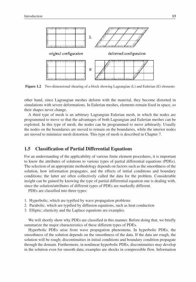
To illustrate this statement, Figure 1.2 shows Lagrangian and Eulerian meshes for the shear deformation given by (1.4.11). As can be seen, a Lagrangian mesh is like an etching on the material: as the material is deformed, the etching (and the elements) deform with it. An Eulerian mesh is like an etching on a sheet of glass held in front of the material: as the material deforms, the etching is unchanged and the material passes across it.

The advantages and disadvantages of the two types of meshes in multi-dimensions are similar to those in one dimension. In Lagrangian meshes, element boundaries (lines in two dimensions, surfaces in three dimensions) remain coincident with boundaries and material interfaces. In Eulerian meshes, element sides do not remain coincident with boundaries or material interfaces. Hence tracking methods or approximate methods, such as volume of fluid approaches, have to be used for moving boundaries treated in Eulerian meshes. Furthermore, an Eulerian mesh must be large enough to enclose the material in its deformed state. On the

0002023647.INDD 12 10/5/2013 11:17:22 AM

Introduction 13

Figure 1.2 Two-dimensional shearing of a block showing Lagrangian (L) and Eulerian (E) elements

other hand, since Lagrangian meshes deform with the material, they become distorted in simulations with severe deformations. In Eulerian meshes, elements remain fixed in space, so their shapes never change.

A third type of mesh is an arbitrary Lagrangian Eulerian mesh, in which the nodes are programmed to move so that the advantages of both Lagrangian and Eulerian meshes can be exploited. In this type of mesh, the nodes can be programmed to move arbitrarily. Usually the nodes on the boundaries are moved to remain on the boundaries, while the interior nodes are moved to minimize mesh distortion. This type of mesh is described in Chapter 7.

1.5 Classification of Partial Differential Equations

For an understanding of the applicability of various finite element procedures, it is important to know the attributes of solutions to various types of partial differential equations (PDEs). The selection of an appropriate methodology depends on factors such as the smoothness of the solution, how information propagates, and the effects of initial conditions and boundary conditions; the latter are often collectively called the data for the problem. Considerable insight can be gained by knowing the type of partial differential equation one is dealing with, since the solution/attributes of different types of PDEs are markedly different.

PDEs are classified into three types:

1. Hyperbolic, which are typified by wave propagation problems2. Parabolic, which are typified by diffusion equations, such as heat conduction3. Elliptic; elasticity and the Laplace equations are examples.

We will shortly show why PDEs are classified in this manner. Before doing that, we briefly summarize the major characteristics of these different types of PDEs.

Hyperbolic PDEs arise from wave propagation phenomena. In hyperbolic PDEs, the smoothness of the solution depends on the smoothness of the data. If the data are rough, the solution will be rough; discontinuities in initial conditions and boundary condition propagate through the domain. Furthermore, in nonlinear hyperbolic PDEs, discontinuities may develop in the solution even for smooth data; examples are shocks in compressible flow. Information

0002023647.INDD 13 10/5/2013 11:17:22 AM

14 Nonlinear Finite Elements for Continua and Structures

in a hyperbolic model travels at a finite speed called the wavespeed. This is illustrated in Figure 1.3, which shows a rod with a force (source) applied at the left-hand end at time t = 0. An observer at a point x will not be aware of the source until the wave reaches him: the wave front is indicated by a line of slope c–1 in Figure 1.3; c is the wavespeed.

Elliptic PDEs are in a sense the opposite of hyperbolic PDEs. Examples of elliptic PDEs are the Laplace equation and the equations of elasticity. In elliptic PDEs the solutions are very smooth, that is, they are analytic, even if the data are rough. Furthermore, boundary data at any point tend to affect the entire solution, that is, the domain of influence of data is the entire domain. However, the effect of small irregularities in boundary data tends to be confined to the boundary: this is known as St Venant’s principle. The major difficulty in the solution of elliptic PDEs is that acute corners in the boundary lead to singularities in the solution. For example, at a re-entrant corner such as a crack, the strains (derivatives of the displacements) in two-dimensional elastic solutions vary like r –½, where r is the distance from the crack tip. This is the well-known crack tip singularity in fracture mechanics.

Parabolic PDEs are time-dependent PDEs with solutions that are smooth in space, but they may possess singularities at corners. Their attributes are intermediate between elliptic and hyperbolic equations. An example of a parabolic equation is the heat conduction equation. Information travels at an infinite speed in a parabolic system. For example, Figure 1.3 shows a heat source applied to a rod. The temperature rises instantaneously along the entire rod according to the heat conduction equation. Far from a source, the temperature increase may be very small. In hyperbolic systems, there is no response until the wave arrives.

The classification of PDEs rests on whether lines or surfaces exist across which the deriva-tives of the solution are discontinuous. This is equivalent to examining whether lines exist along which the PDEs can be reduced to ordinary differential equations.

The classification of PDEs is usually developed for first-order systems (any second-order system can be expressed as two first-order systems). Consider a quasilinear system in two unknowns:

1 1 1 1 1, , , ,x y x yA u B u C v D v E+ + + = (1.5.1)

2 2 2 2 2, , , ,x y x yA u B u C v D v E+ + + = (1.5.2)

Figure 1.3 Flow of information in parabolic and hyperbolic systems of PDEs

0002023647.INDD 14 10/5/2013 11:17:23 AM

Introduction 15

In the above Ai, B

i, C

i and D

i are functions of the independent variables x and y and of the two

dependent variables u(x, y) and v(x, y). The system is called quasilinear because it is linear in the derivatives.

Now let’s examine whether u and v can have discontinuous derivatives in the x–y plane. Consider a curve Γ parametrized by s. Along Γ the derivatives are continuous but across Γ the derivatives may be discontinuous. By the chain rule, the derivatives of the dependent variables can be written as

= + = +, , , , , , , , , ,s x s y s s x s y su u x u y v v x v y (1.5.3)

Writing (1.5.1–1.5.3) as a single matrix equation gives

= =

1 1 1 1 1

2 2 2 2 2

,

,

, , 0 0 ,,

0 0 , , ,,

x

y

s s sx

s s sy

uA B C D EuA B C D E

x y uv

x y vv

Az (1.5.4)

If the derivatives are discontinuous, the solution of the above system of linear algebraic equations is indeterminate, that is, the solution is nonunique, which implies det(A) = 0. Enforcing this condition yields (after some algebra):

2 2, 2 , , , 0s s s say bx y cx+ + = (1.5.5)

where

= =2 1 1 2 2 1 1 2– , –a A C A C c B D B D (1.5.6)

= +1 2 2 1 1 2 2 12 – –b B C B C A D A D

Dividing (1.5.5) by 2,xx and noting that y,s / x,

s = dy / dx ≡ y,

x we obtain

+ + =2, 2 , 0x xay by c (1.5.7)

The solution to (1.5.7) is given by the roots of the quadratic equation

− ± −=2

,b b ac

y xa

(1.5.8)

The solution of the above gives the lines Γ along which the solutions may have discontinuous derivatives. If b2 – ac < 0, then y,

x is imaginary and such lines do not exist. If b2 – ac > 0, these

lines are real, so discontinuities can exist; such PDEs are called hyperbolic.Since y,

x by (1.5.8) is determined by the roots of a quadratic equation, there are two roots,

which give two sets of lines Γ+ and Γ–, as shown in Figure  1.4. These lines are called characteristics. The classification of PDEs is summarized in Table 1.1. For time-dependent problems, the characteristics are lines along which information propagates in the x–t plane; the slope of these lines is the instantaneous wave speed c.

0002023647.INDD 15 10/5/2013 11:17:25 AM

16 Nonlinear Finite Elements for Continua and Structures

As an example, we consider the one-dimensional wave equation

= 2, ,tt xxu c u (1.5.9)

To reduce this equation to first-order form (1.5.1–2) we let f = u,x, g = u,

t. The wave equation

then becomes a set of two first-order equations:

= =2, , , ,t x t xg c f f g (1.5.10)

where the second equation is just the statement u,xt = u,

tx. Writing the above system in matrix

form with (1.5.4) gives

2

0 1 1 0

0 0 1, [ , , , , ]

, , 0 0

0 0 , ,

Tx t x t

s s

s s

cf f g g

x y

x y

− − = =

A z (1.5.11)

The characteristics are then found by setting det (A) = 0, which gives

2 2 2 2 2, , 0 or ,s s tx c t x c− = = (1.5.12)

Figure 1.4 Characteristics in a hyper bolic system

Table 1.1 Classification of PDEs

b2 – ac PDE Classification Solution smoothness

> 0 has two families of characteristics hyperbolic discontinuous derivatives= 0 has one family of characteristics parabolic smooth< 0 no real characteristic elliptic smooth

0002023647.INDD 16 10/5/2013 11:17:27 AM

Introduction 17

From this it can be seen that the PDE is hyperbolic. The two sets of characteristic lines are given by

= ±,tx c (1.5.13)

The characteristics are thus lines with slope ±c–1 in the x–t plane. In other words, in the wave equation information travels to the left or right by the wave speed. Across the characteristic lines, the derivatives of f = u,

x = e

x (e

x is the linear strain) and of g = u,

t (the velocity) can be

discontinuous.Consider next the Laplace equation G

1u,

xx + G

2u,

yy = 0. This is the governing equation for

the elastic antiplane problem; u(x, y) is the displacement in the z direction and Ga are the shear moduli. The procedure for examining the character of this equation is identical to that given before. The steps are sketched in the following:

1 2

0 1 1 0

0 0, , , , , [ , , , ,

, , 0 0

0 0 ,

]

,

Tx y x y x y

s s

s s

G Gf u g u f f g g

x t

x t

− = = = =

A z

(1.5.14)

det(A) = 0 implies 2 2 2 11 2

2

, , 0 or ,s s x

GG x G y y

G+ = = − (1.5.15)

If G1 > 0 and G

2 > 0 (which is the case for stable elastic materials), the characteristic lines are

then imaginary and the system is elliptic. No discontinuities are possible in the derivatives f ≡ u,

x or g ≡ u,

y. Discontinuities in derivatives are possible when the material constants Ga are

not homogeneous, that is, when the coefficients of the PDE Ga are discontinuous. However, discontinuities in derivatives of u coincide with the discontinuities in Ga. This equation differs from the wave equation in that both independent variables are spatial coordinates; it is difficult to give simple examples of PDEs in space-time which are elliptic.

It is left as an exercise to show that the equation u,t = αu,

xx is parabolic. In a parabolic

system, only one set of characteristics exists. These are parallel to the time axis, so information travels at infinite speed. In parabolic systems, discontinuities occur in space only if there are discontinuities in the data.

In a hyperbolic system, the governing equations become ordinary differential equations along the characteristics. By integrating these ODEs along the characteristics, very accurate solutions to hyperbolic PDEs can be obtained. This method is called the method of character-istics. Such methods are very appealing because of their high accuracy. However, they are quite difficult to program for more than one space dimension for arbitrary constitutive laws, so the method of characteristics is used only in special-purpose software.

1.6 Exercises

1.1. Show that the diffusion equation (heat conduction is one example) u,xx

= αu,t, where a is

a positive constant, is parabolic.1.2. Determine the classification of the equation for the dynamics of beams, u,

xxxx = αu,

tt.

0002023647.INDD 17 10/5/2013 11:17:28 AM

0002023647.INDD 18 10/5/2013 11:17:28 AM