Embed Size (px)
Citation preview
IAT 355 Visual Analytics
Show Me the Numbers Lyn Bartram

Administrivia
• In-class exercise Thursday • Visualization in practice • Find one good and one bad example • Put on Canvas discussion • Present BRIEFLY in class • We’ll need to run over • We will revisit these choices later!
• Assignment 1 issues – contact Ankit/lyn directly
Working with Data | IAT 4355 2
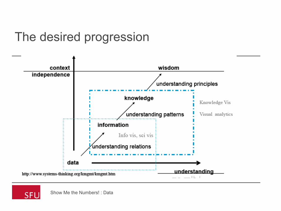
The desired progression
Show Me the Numbers! : Data

Another way of looking at it ….
Show Me the Numbers! : Data

Visualization Stages Data
Working with Data | IAT 4355 5
Raw Informa+on
Visual Form Dataset Views
User - Task
Data Transformations
Visual Mappings
View Transformations
F F -‐1
Interac+on
Visual Perception
Visual Form
Task

Visualization Stages Data transformation – create a visual spatial model
• Data transformation • Map raw data into data tables – e.g. text to similarity matrix
Working with Data | IAT 4355 6
Raw Informa+on
Visual Form Dataset Views
User - Task
Data Transformations
Visual Mappings
View Transformations
F F -‐1
Interac+on
Visual Perception

Visualization Stages Visual mapping– create a visual spatial model
• Data transformation • Map raw data into data tables – e.g. text to similarity matrix
• Visual Mappings: • Transform data tables into visual structures – e.g., house price,
#bedrooms to 2 dims – x, y
Working with Data | IAT 4355 7
Raw Informa+on
Visual Form Dataset Views
User - Task
Data Transformations
Visual Mappings
View Transformations
F F -‐1
Interac+on
Visual Perception
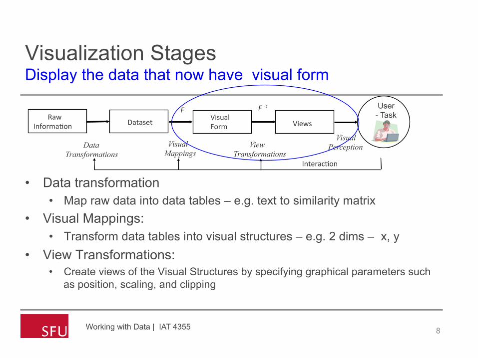
Visualization Stages Display the data that now have visual form
• Data transformation • Map raw data into data tables – e.g. text to similarity matrix
• Visual Mappings: • Transform data tables into visual structures – e.g. 2 dims – x, y
• View Transformations: • Create views of the Visual Structures by specifying graphical parameters such
as position, scaling, and clipping
Working with Data | IAT 4355 8
Raw Informa+on
Visual Form Dataset Views
User - Task
Data Transformations
Visual Mappings
View Transformations
F F -‐1
Interac+on
Visual Perception
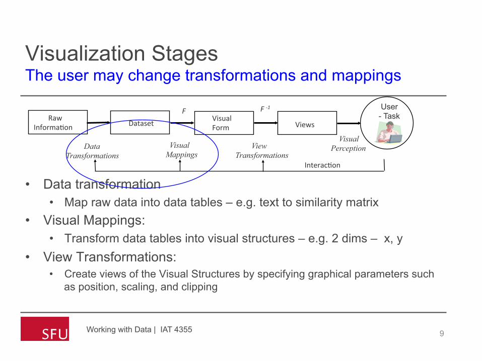
Visualization Stages The user may change transformations and mappings
• Data transformation • Map raw data into data tables – e.g. text to similarity matrix
• Visual Mappings: • Transform data tables into visual structures – e.g. 2 dims – x, y
• View Transformations: • Create views of the Visual Structures by specifying graphical parameters such
as position, scaling, and clipping
Working with Data | IAT 4355 9
Raw Informa+on
Visual Form Dataset Views
User - Task
Data Transformations
Visual Mappings
View Transformations
F F -‐1
Interac+on
Visual Perception

What are we looking at? For?
Show Me the Numbers! : Data
DATA ??

But WHAT numbers?????
• Data Models
• Types
• Metadata
• Descriptive Statistics
• Distribution
• Clusters
Show Me the Numbers! : Data
Data forms
• Data comes in many different forms • Typically, not in the way you want it
• Data concerns • Formats and types
• Marshalling • Structure and relations • Purpose /analytical aggregation

Data models
• Often, we take raw data and transform it into a form that is more workable
• Main idea: build a model • Individual items are called cases or records • Cases have attributes : an attribute is a value of a
variable or factor • In vis terms, a dimension
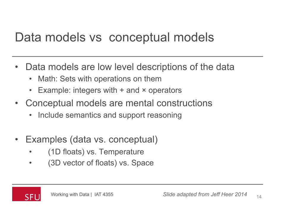
Data models vs conceptual models
• Data models are low level descriptions of the data • Math: Sets with operations on them • Example: integers with + and × operators
• Conceptual models are mental constructions • Include semantics and support reasoning
• Examples (data vs. conceptual) • � (1D floats) vs. Temperature • � (3D vector of floats) vs. Space
Working with Data | IAT 4355 14 Slide adapted from Jeff Heer 2014
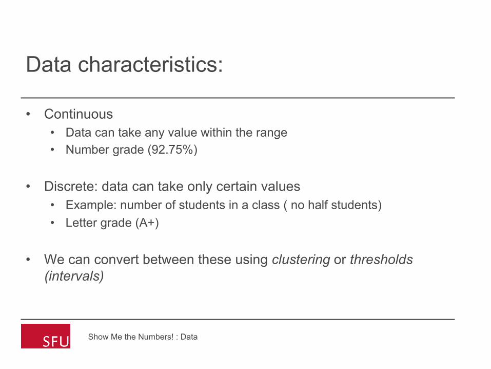
Data characteristics:
• Continuous • Data can take any value within the range • Number grade (92.75%)
• Discrete: data can take only certain values • Example: number of students in a class ( no half students) • Letter grade (A+)
• We can convert between these using clustering or thresholds (intervals)
Show Me the Numbers! : Data

Variables (factor) types
• Physical • Characterised by storage format • Chacracterised by machine operations • Boolean, short, int32,float, double,string, text, number …
• Abstract types • Provide descriptions of the data • May be characterised by methods/attributes • May be organised into a hierarchy • Plants, animals,
Working with Data | IAT 4355 16 Slide adapted from Jeff Heer 2014
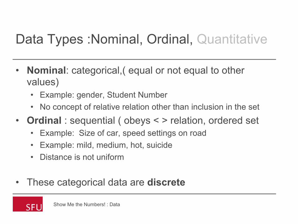
Data Types :Nominal, Ordinal, Quantitative
• Nominal: categorical,( equal or not equal to other values) • Example: gender, Student Number • No concept of relative relation other than inclusion in the set
• Ordinal : sequential ( obeys < > relation, ordered set • Example: Size of car, speed settings on road • Example: mild, medium, hot, suicide • Distance is not uniform
• These categorical data are discrete
Show Me the Numbers! : Data

Data Types : Nominal, Ordinal, Quantitative
• Interval : Relative measurements, no fixed zero point. • Data is numerical, not categorical. Rank order among variables
is explicit with an equal spread between points in the data set: -2, -1, 0, +1, +2
• Example: distance, hours in a day
• Ratio: Zero fixed • Example: account balance • Can measure ratios or proportions
• Usually continuous to some sampling level
Show Me the Numbers! : Data

Data types
• Quantitative i.e. numerical • Continuous (e.g. pH of a sample, patient cholesterol levels) • Discrete (e.g. number of bacteria colonies in a culture)
• Categorical • Nominal (e.g. gender, blood group) • Ordinal (ranked e.g. mild, moderate or severe illness). Often
ordinal variables are re-coded to be quantitative. • This assigns weights or priorities.
19
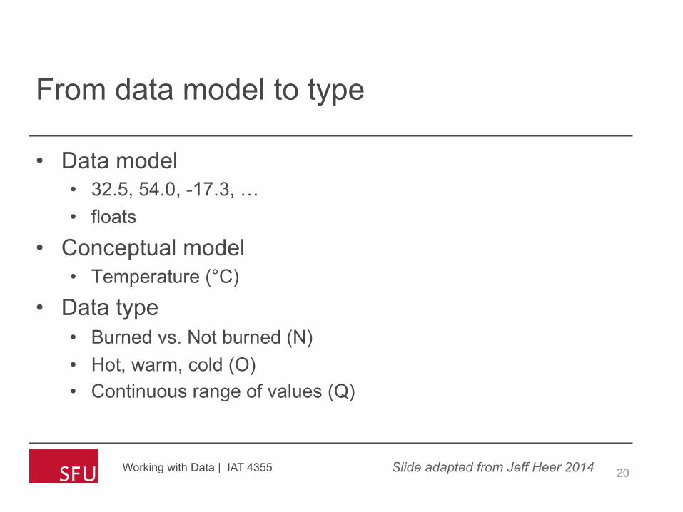
From data model to type
• Data model • 32.5, 54.0, -17.3, … • floats
• Conceptual model • Temperature (°C)
• Data type • Burned vs. Not burned (N) • Hot, warm, cold (O) • Continuous range of values (Q)
Working with Data | IAT 4355 20 Slide adapted from Jeff Heer 2014
Slide adapted from Jeff Heer 2014
From data model to type
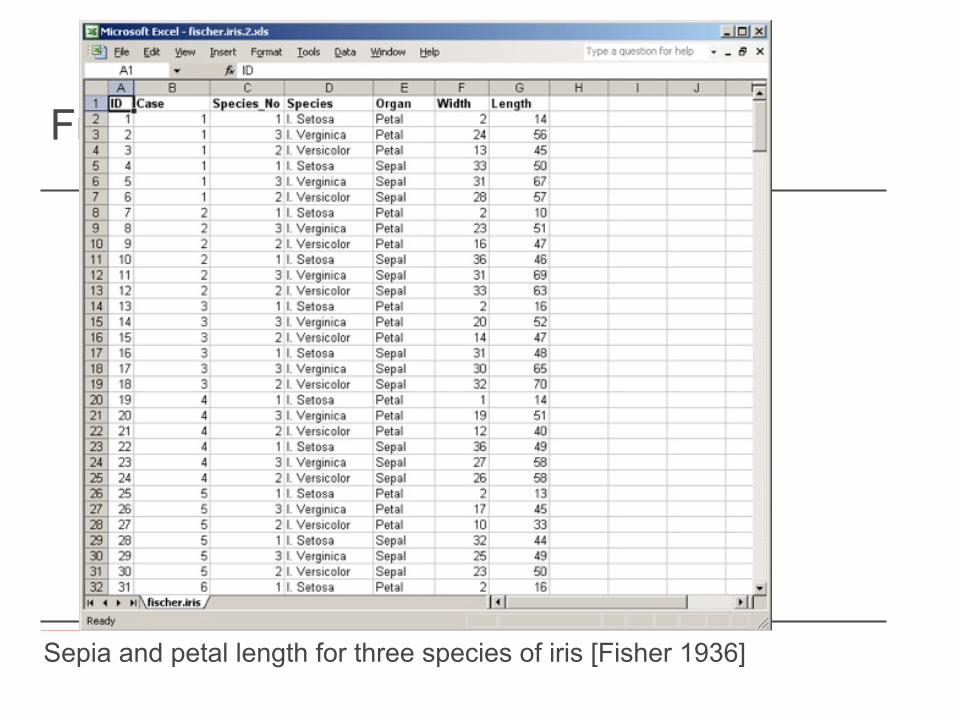
Working with Data | IAT 4355 21 Sepia and petal length for three species of iris [Fisher 1936]

From data model to type
Working with Data | IAT 4355 22 Slide adapted from Jeff Heer 2014
Q O N
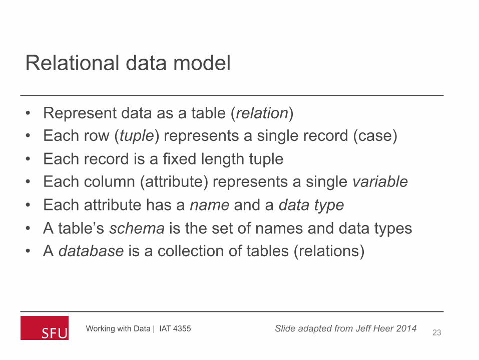
Relational data model
• Represent data as a table (relation) • Each row (tuple) represents a single record (case) • Each record is a fixed length tuple • Each column (attribute) represents a single variable • Each attribute has a name and a data type • A table’s schema is the set of names and data types • A database is a collection of tables (relations)
Working with Data | IAT 4355 23 Slide adapted from Jeff Heer 2014

Show Me the Numbers! : Data
Data Table Format
• Think of this as a function ■ if(case1) = <Val11, Val12,…>
Case1 Case2 Case3
Variable1 Value11 Value21 Value31
Variable2 Value12 Value22 Value32
Variable3 Value13 Value23 Value33
Dimensions
Example: Student Data
Show Me the Numbers! : Data
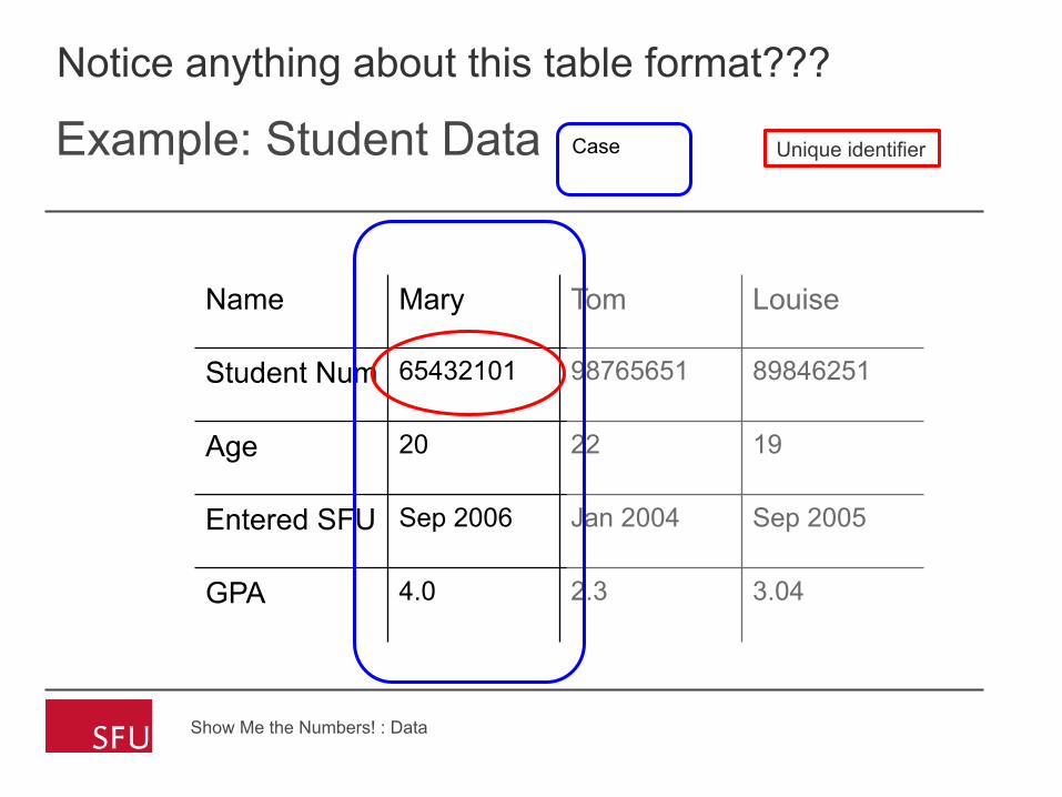
Name Mary Tom Louise
Student Num 65432101 98765651 89846251
Age 20 22 19
Entered SFU Sep 2006 Jan 2004 Sep 2005
GPA 4.0 2.3 3.04
Case
Notice anything about this table format???
Unique identifier
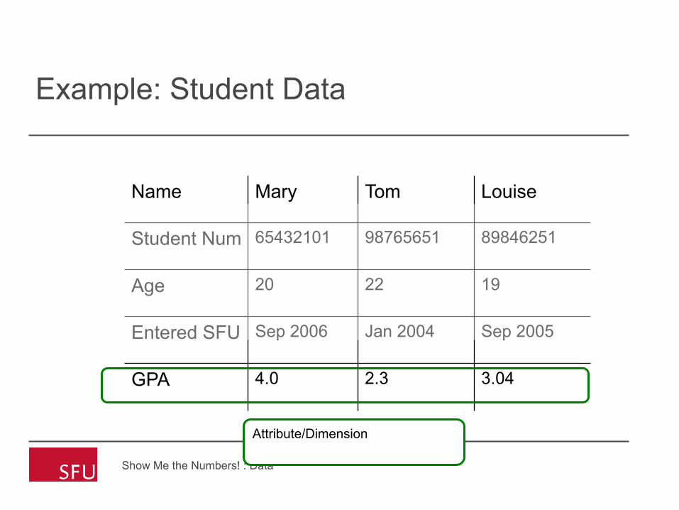
Example: Student Data
Show Me the Numbers! : Data
Name Mary Tom Louise
Student Num 65432101 98765651 89846251
Age 20 22 19
Entered SFU Sep 2006 Jan 2004 Sep 2005
GPA 4.0 2.3 3.04
Attribute/Dimension

Example: What kinds of data? Types?
Show Me the Numbers! : Data
Name Mary Tom Louise
Student Num 65432101 98765651 89846251
Age 20 22 19
Entered SFU Sep 2006 Jan 2004 Sep 2005
GPA 4.0 2.3 3.04 Date, interval, point, term – underlying data, current format

How many dimensions?
• Data sets of dimensions 1, 2, 3 are common
• Number of variables per case • 1 - Univariate data • 2 - Bivariate data • 3 - Trivariate data • >3 - Hypervariate data
• These are the fun and interesting ones! But hard!
Show Me the Numbers! : Data

Issues to consider
• Spatial/temporal frequencies on data • Missing values
• Interpolate • Show as missing explicitly? • Ignore?
• Special values • Of particular interest to visualize • Thresholds, ratio scales (consider sea level relative values)
Show Me the Numbers! : Data

But wait…. There’s more !
• Raw data
• Metadata • Data about the data • GPS, Time, Lens aperture, source …..
• Frequency data • “more than half the respondents smoked before 16”
• Derived data • Summaries, observations, inferences, predictions • “the odds of you getting ill from this pizza were 5 to 1”
Show Me the Numbers! : Data
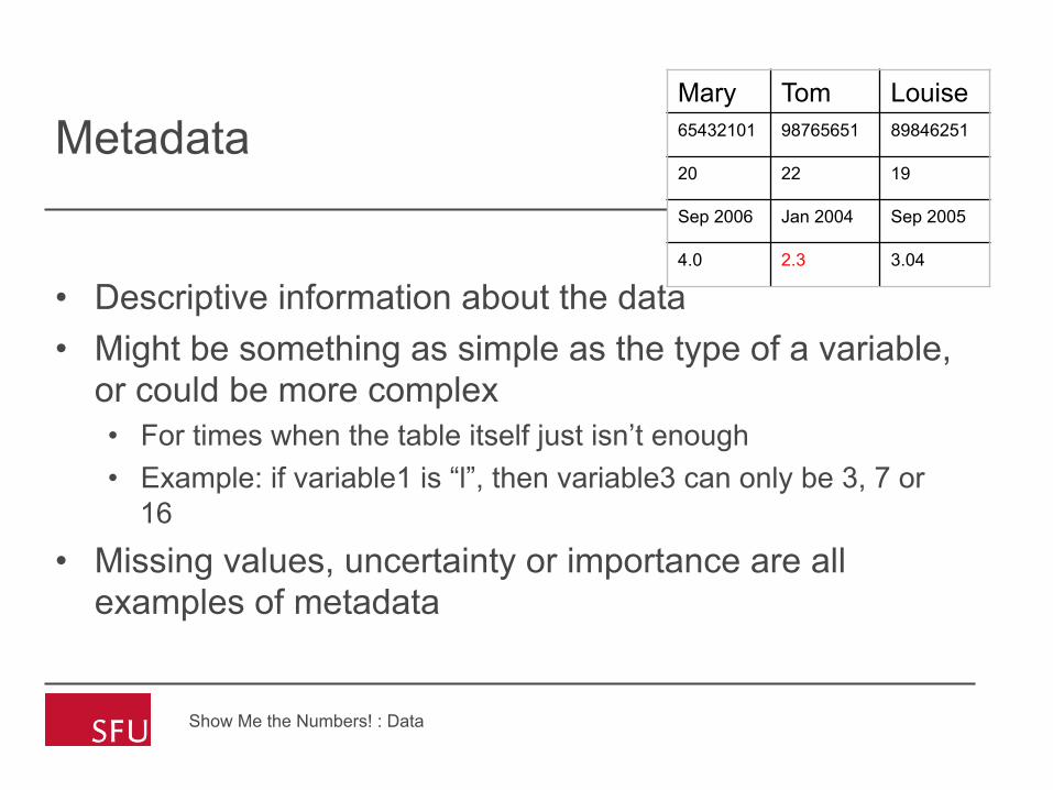
Metadata
• Descriptive information about the data • Might be something as simple as the type of a variable,
or could be more complex • For times when the table itself just isn’t enough • Example: if variable1 is “l”, then variable3 can only be 3, 7 or
16
• Missing values, uncertainty or importance are all examples of metadata
Show Me the Numbers! : Data
Mary Tom Louise 65432101 98765651 89846251
20 22 19
Sep 2006 Jan 2004 Sep 2005
4.0 2.3 3.04
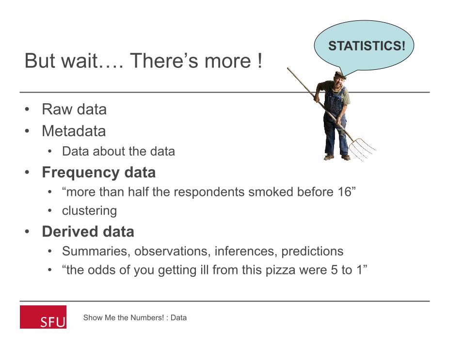
But wait…. There’s more !
• Raw data • Metadata
• Data about the data
• Frequency data • “more than half the respondents smoked before 16” • clustering
• Derived data • Summaries, observations, inferences, predictions • “the odds of you getting ill from this pizza were 5 to 1”
Show Me the Numbers! : Data
STATISTICS!
33
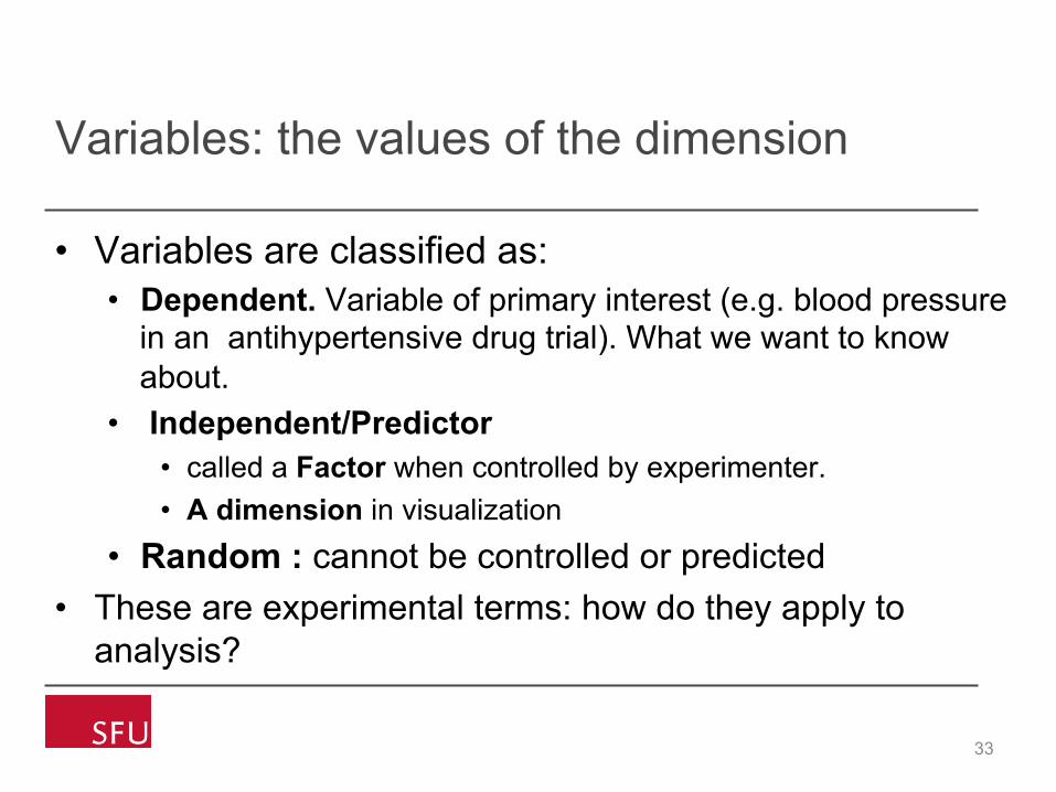
Variables: the values of the dimension
• Variables are classified as: • Dependent. Variable of primary interest (e.g. blood pressure
in an antihypertensive drug trial). What we want to know about.
• Independent/Predictor • called a Factor when controlled by experimenter. • A dimension in visualization
• Random : cannot be controlled or predicted • These are experimental terms: how do they apply to
analysis?

Statistical data models
• Observations or cases
• Categories, factors, dimensions • Discrete variables describing the data • Dates, categories of values (independent variables)
• Measures: Data values that can be aggregated • Numbers to be analyzed (dependent variables) • Aggregate as sum, count, average, std. deviation, …
Working with Data | IAT 4355 34
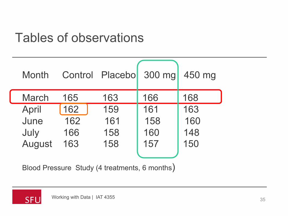
Tables of observations
Working with Data | IAT 4355 35
Month Control Placebo 300 mg 450 mg March 165 163 166 168 April 162 159 161 163 June 162 161 158 160 July 166 158 160 148 August 163 158 157 150 Blood Pressure Study (4 treatments, 6 months)
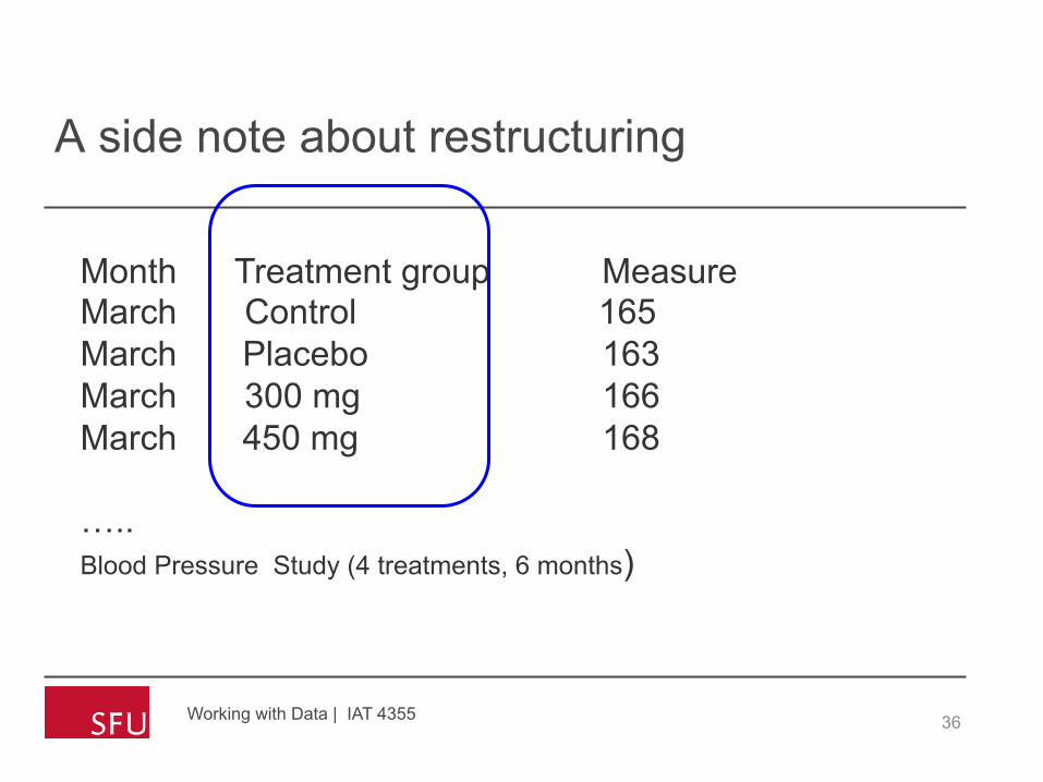
A side note about restructuring
Working with Data | IAT 4355 36
Month Treatment group Measure March Control 165 March Placebo 163 March 300 mg 166 March 450 mg 168 ….. Blood Pressure Study (4 treatments, 6 months)

Data analysis
• Qualitative • Descriptive. Used to describe the distribution of a
single variable or the relationship between two nominal variables (mean, frequencies, cross-tabulation)
• Inferential (Used to establish relationships among variables; assumes random sampling and a normal distribution)
• Nonparametric (Used to establish causation for small samples or data sets that are not normally distributed)
Show Me the Numbers! : Data
Descriptive Statistics: Univariate
• Range • Min/Max • Average • Median • Mode
Show Me the Numbers! : Data
Distribution Statistics
• Variance • Error • Standard Deviation • Histograms and Normal Distributions
Show Me the Numbers! : Data

Frequency statistics
Most basic type of descriptive statistic
• An (Empirical) Frequency Distribution for a continuous variable presents the counts of observations grouped within pre-specified classes or groups
• A Relative Frequency Distribution presents the corresponding proportions of observations within the classes
• Visualizations: barcharts, histograms Show Me the Numbers! : Data

Example use of frequency
• 40% of respondents are male. • The mean level of income was $35,000 • 40% of all female voters cast their vote for Arnold compared to
52% of the male voters.
Show Me the Numbers! : Data
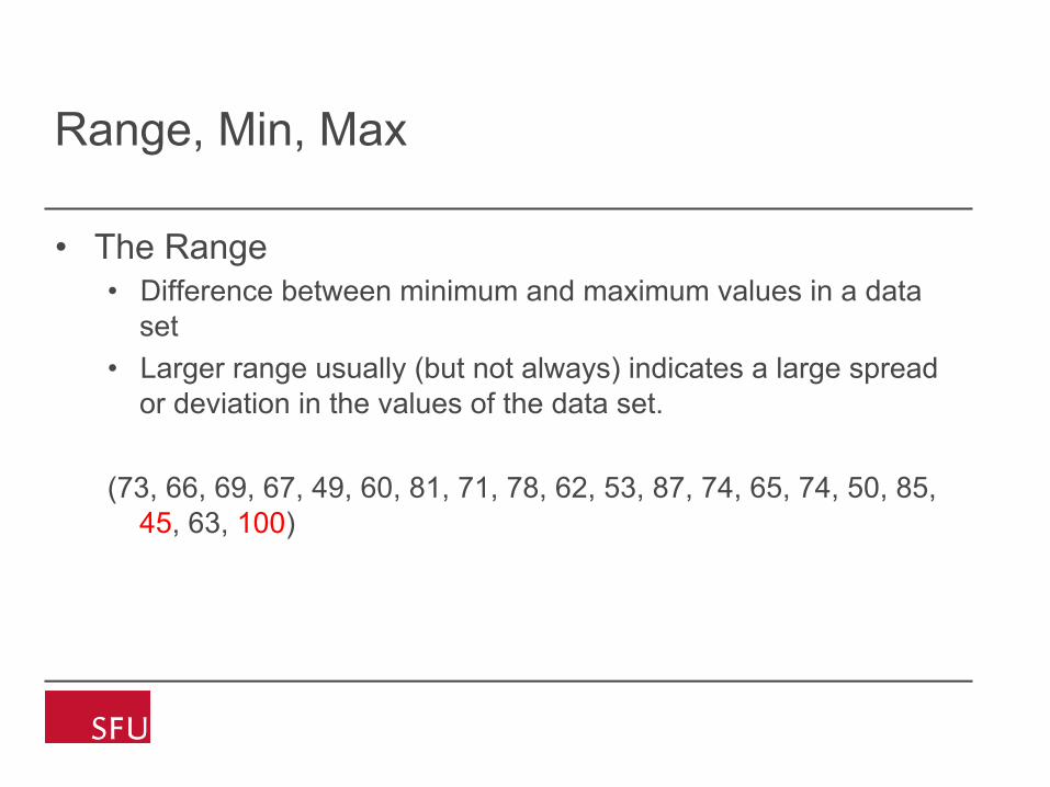
• The Range • Difference between minimum and maximum values in a data
set • Larger range usually (but not always) indicates a large spread
or deviation in the values of the data set.
(73, 66, 69, 67, 49, 60, 81, 71, 78, 62, 53, 87, 74, 65, 74, 50, 85, 45, 63, 100)
Range, Min, Max
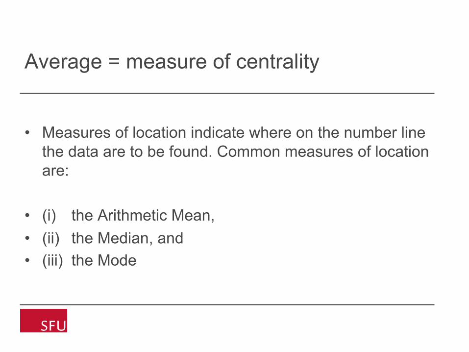
Average = measure of centrality
• Measures of location indicate where on the number line the data are to be found. Common measures of location are:
• (i) the Arithmetic Mean, • (ii) the Median, and • (iii) the Mode
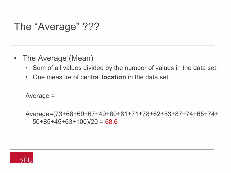
• The Average (Mean) • Sum of all values divided by the number of values in the data set. • One measure of central location in the data set.
Average = Average=(73+66+69+67+49+60+81+71+78+62+53+87+74+65+74+
50+85+45+63+100)/20 = 68.6
The “Average” ???
The tyranny of the mean
• When might you not want to use the mean?
Show Me the Numbers! : Data

The mean is vulnerable to problems
0 2.5 7.5 10
4.8
0 2.5 7.5 10
4.8
The data may or may not be symmetrical around its average value
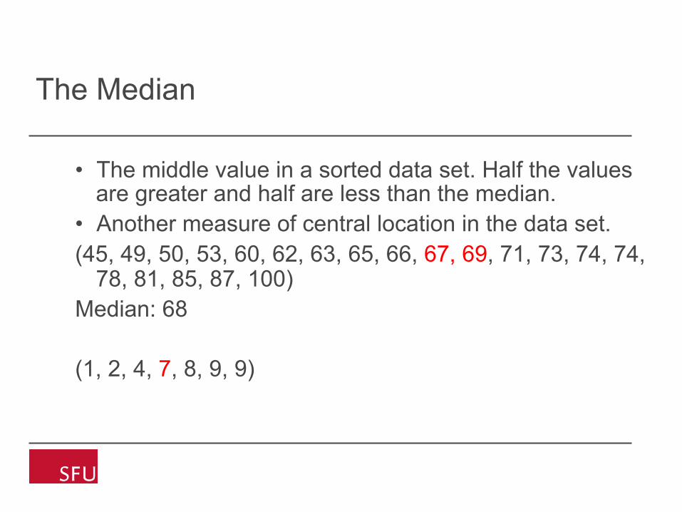
• The middle value in a sorted data set. Half the values are greater and half are less than the median.
• Another measure of central location in the data set. (45, 49, 50, 53, 60, 62, 63, 65, 66, 67, 69, 71, 73, 74, 74,
78, 81, 85, 87, 100) Median: 68 (1, 2, 4, 7, 8, 9, 9)
The Median
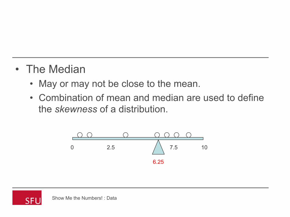
• The Median • May or may not be close to the mean. • Combination of mean and median are used to define
the skewness of a distribution.
Show Me the Numbers! : Data
0 2.5 7.5 10
6.25

The Mode
• The most frequent occurring value. • Another measure of central location in the data
set. • (45, 49, 50, 53, 60, 62, 63, 65, 66, 67, 69, 71,
73, 74, 74, 78, 81, 85, 87, 100) • Mode: 74 • Generally not all that meaningful unless a larger
percentage of the values are the same number
Show Me the Numbers! : Data

When do we use what?
• Dependent on how the data are distributed • Note if mean=median=mode then
the data are said to be symmetrical • Rule of thumb:
• use mean if data are normally distributed and variance is within constraints
• Use median to reduce effects of outliers
Show Me the Numbers! : Data
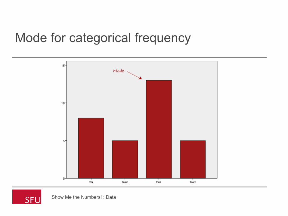
Mode for categorical frequency
Show Me the Numbers! : Data

Summary
Show Me the Numbers! : Data
http://statistics.laerd.com/statistical-guides/measures-central-tendency-mean-mode-median.php
Data distribution
• Measures of dispersion characterise how spread out the distribution is, i.e., how variable the data are.
• Commonly used measures of dispersion include: 1. Range 2. Variance & Standard deviation 3. Coefficient of Variation (or relative standard deviation) 4. Inter-quartile range
Show Me the Numbers! : Data

Measures of variance
• Variance • One measure of dispersion (deviation from the mean) of a data
set. The larger the variance, the greater is the average deviation of each datum from the average value
• Standard Deviation • the average deviation from the mean of a data set.
• Variance and SD are critical in analysing your data distribution and determining how “meaningful” is the chosen average
Show Me the Numbers! : Data
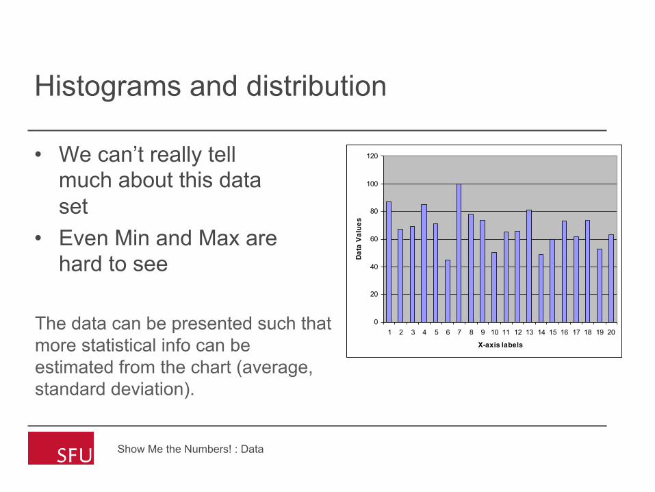
Histograms and distribution
• We can’t really tell much about this data set
• Even Min and Max are hard to see
Show Me the Numbers! : Data
0
20
40
60
80
100
120
1 2 3 4 5 6 7 8 9 10 11 12 13 14 15 16 17 18 19 20
X-axis labels
Data
Val
ues
The data can be presented such that more statistical info can be estimated from the chart (average, standard deviation).

Plotting the distribution
• Determine a frequency table (bins) • A histogram is a column chart of the frequencies
Show Me the Numbers! : Data
Category Labels Frequency 0-50 3
51-60 2 61-70 6 71-80 5 81-90 3 >90 1 0
1
2
3
4
5
6
7
0-50 51-60 61-70 71-80 81-90 >90
Scores
Frequency

Data Mining Lectures Lecture on EDA and Visualization Padhraic Smyth, UC Irvine
Histogram
• Most common form: split data range into equal-sized bins Then for each bin, count the number of points from the data set that fall into the bin. • Vertical axis: Frequency (i.e., counts for each bin) • Horizontal axis: Response variable
• The histogram graphically shows the following: 1. center (i.e., the location) of the data; 2. spread (i.e., the scale) of the data; 3. skewness of the data; 4. presence of outliers; and 5. presence of multiple modes in the data.
Data Mining Lectures Lecture on EDA and Visualization Padhraic Smyth, UC Irvine
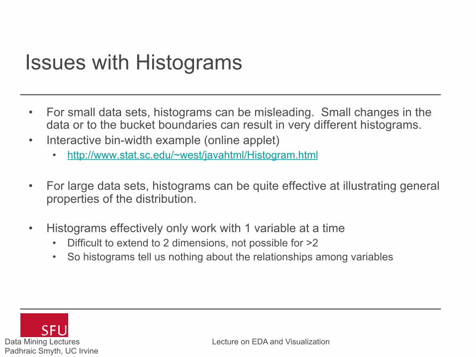
Issues with Histograms
• For small data sets, histograms can be misleading. Small changes in the data or to the bucket boundaries can result in very different histograms.
• Interactive bin-width example (online applet) • http://www.stat.sc.edu/~west/javahtml/Histogram.html
• For large data sets, histograms can be quite effective at illustrating general
properties of the distribution.
• Histograms effectively only work with 1 variable at a time • Difficult to extend to 2 dimensions, not possible for >2 • So histograms tell us nothing about the relationships among variables

Normal and Skewed Distributions
• When data are skewed, the mean and SD can be misleading
• Skewness sk= 3(mean-median)/SD If sk>|1| then distribution is non-
symetrical • Negatively skewed
• Mean<Median • Sk is negative
• Positively Skewed • Mean>Median • Sk is positive
Show Me the Numbers! : Data
0
0.02
0.04
0.06
0.08
0.1
0.12
0.14
0 20 40 60 80 100 120 140 160
0
0.02
0.04
0.06
0.08
0.1
0.12
25 45 65 85 105 125 145 165 185 205 225

60
Inter-quartile range
• The Median divides a distribution into two halves.
• The first and third quartiles (denoted Q1 and Q3) are defined as follows: • 25% of the data lie below Q1 (and 75% is above Q1),
• 25% of the data lie above Q3 (and 75% is below Q3)
• The inter-quartile range (IQR) is the difference between the first and third quartiles, i.e. IQR = Q3- Q1
61
Box-plots
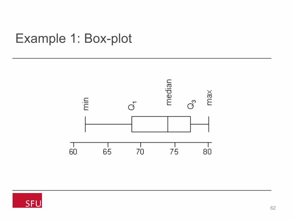
• A box-plot is a visual description of the distribution based on • Minimum • Q1 • Median • Q3 • Maximum
• Useful for comparing large sets of data
62
Example 1: Box-plot
63
Outliers
• An outlier is an datum which does not appear to belong with the other data
• Outliers can arise because of a measurement or recording error or because of equipment failure during an experiment, etc.
• An outlier might be indicative of a sub-population, e.g. an abnormally low or high value in a medical test could indicate presence of an illness in the patient.

64
Outlier Boxplot
• Re-define the upper and lower limits of the boxplots (the whisker lines) as: Lower limit = Q1-1.5×IQR, and Upper limit = Q3+1.5×IQR
• Note that the lines may not go as far as these limits
• If a data point is < lower limit or >
upper limit, the data point is considered to be an outlier.
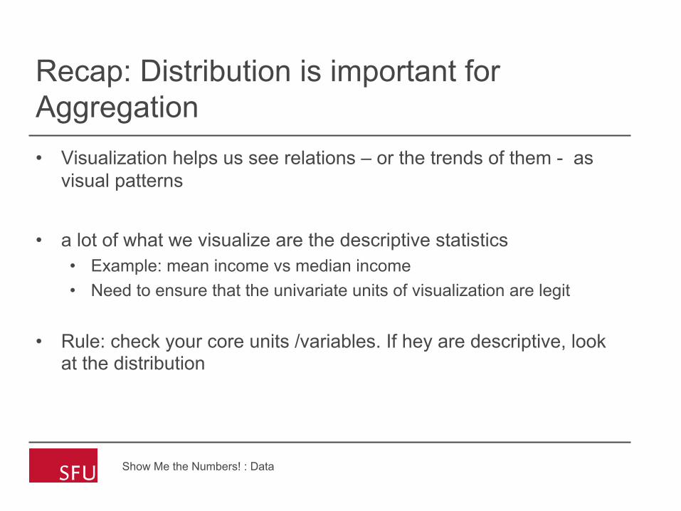
Recap: Distribution is important for Aggregation • Visualization helps us see relations – or the trends of them - as
visual patterns
• a lot of what we visualize are the descriptive statistics • Example: mean income vs median income • Need to ensure that the univariate units of visualization are legit
• Rule: check your core units /variables. If hey are descriptive, look at the distribution
Show Me the Numbers! : Data

Example: job losses in US over time
Show Me the Numbers! : Data
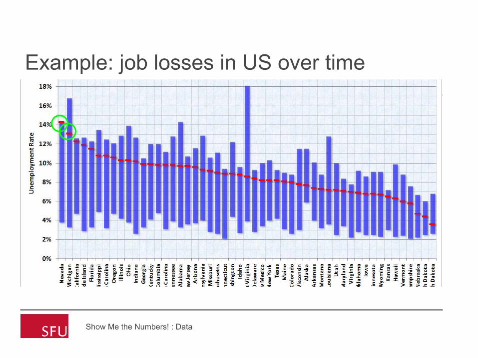
Example: job losses in US over time
Show Me the Numbers! : Data

Show Me the Numbers! : Data