1

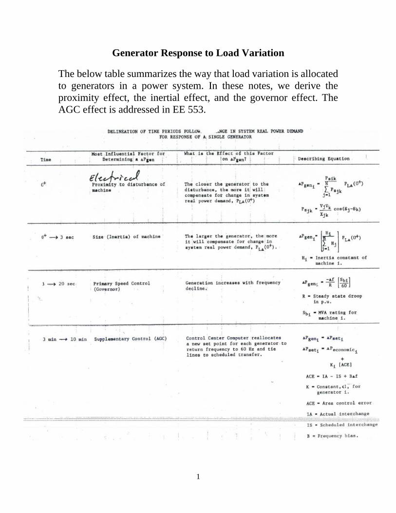
Generator Response to Load Variation

The below table summarizes the way that load variation is allocated

to generators in a power system. In these notes, we derive the

proximity effect, the inertial effect, and the governor effect. The

AGC effect is addressed in EE 553.

2

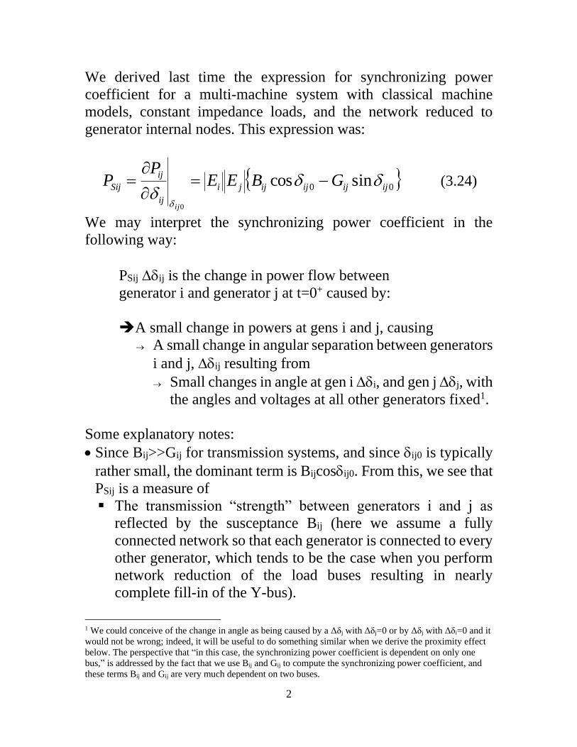
We derived last time the expression for synchronizing power

coefficient for a multi-machine system with classical machine

models, constant impedance loads, and the network reduced to

generator internal nodes. This expression was:

00 sincos

0

ijijijijji

ij

ij

Sij GBEEP

P

ij

(3.24)

We may interpret the synchronizing power coefficient in the

following way:

PSij ij is the change in power flow between

generator i and generator j at t=0+ caused by:

A small change in powers at gens i and j, causing

A small change in angular separation between generators

i and j, ij resulting from

Small changes in angle at gen i i, and gen j j, with

the angles and voltages at all other generators fixed1.

Some explanatory notes:

Since Bij>>Gij for transmission systems, and since ij0 is typically

rather small, the dominant term is Bijcosij0. From this, we see that

PSij is a measure of

The transmission “strength” between generators i and j as

reflected by the susceptance Bij (here we assume a fully

connected network so that each generator is connected to every

other generator, which tends to be the case when you perform

network reduction of the load buses resulting in nearly

complete fill-in of the Y-bus).

1 We could conceive of the change in angle as being caused by a Δδj with Δδj=0 or by Δδj with Δδi=0 and it

would not be wrong; indeed, it will be useful to do something similar when we derive the proximity effect

below. The perspective that “in this case, the synchronizing power coefficient is dependent on only one

bus,” is addressed by the fact that we use Bij and Gij to compute the synchronizing power coefficient, and

these terms Bij and Gij are very much dependent on two buses.

3

The degree to which the angles of gens i and j are the same.

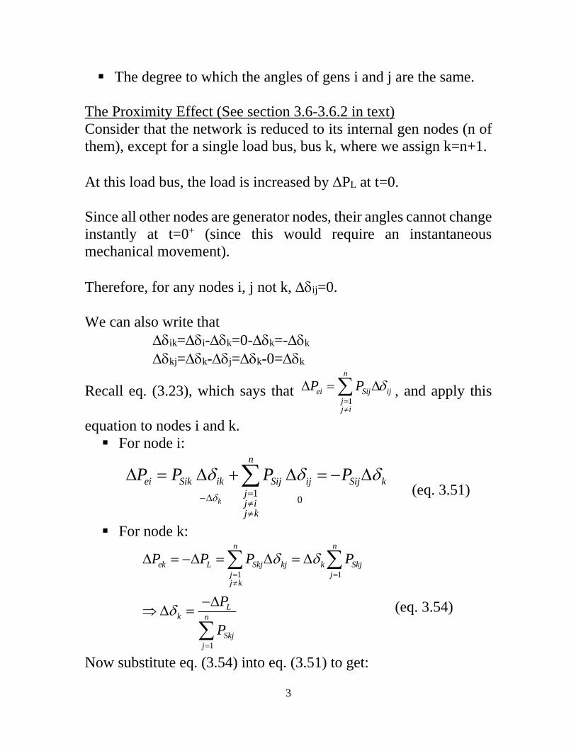
The Proximity Effect (See section 3.6-3.6.2 in text)

Consider that the network is reduced to its internal gen nodes (n of

them), except for a single load bus, bus k, where we assign k=n+1.

At this load bus, the load is increased by PL at t=0.

Since all other nodes are generator nodes, their angles cannot change

instantly at t=0+ (since this would require an instantaneous

mechanical movement).

Therefore, for any nodes i, j not k, ij=0.

We can also write that

ik=i-k=0-k=-k

kj=k-j=k-0=k

Recall eq. (3.23), which says that 1

n

ei Sij ij

jj i

P P

, and apply this

equation to nodes i and k.

For node i:

10k

n

ei Sik ik Sij ij Sij k

jj ij k

P P P P

(eq. 3.51)

For node k:

1 1

1

n n

ek L Skj kj k Skj

j jj k

Lk n

Skj

j

P P P P

P

P

(eq. 3.54)

Now substitute eq. (3.54) into eq. (3.51) to get:

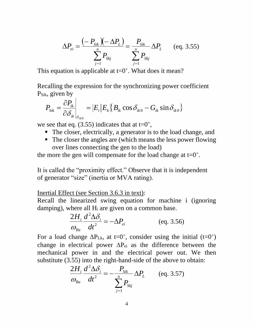
4

Ln

j

Skj

Sik

n

j

Skj

LSikei P

P

P

P

PPP

11

(eq. 3.55)

This equation is applicable at t=0+. What does it mean?

Recalling the expression for the synchronizing power coefficient

PSik, given by

00 sincos

0

ikikikikki

ik

ikSik GBEE

PP

ik

we see that eq. (3.55) indicates that at t=0+,

The closer, electrically, a generator is to the load change, and

The closer the angles are (which means the less power flowing

over lines connecting the gen to the load)

the more the gen will compensate for the load change at t=0+.

It is called the “proximity effect.” Observe that it is independent

of generator “size” (inertia or MVA rating).

Inertial Effect (see Section 3.6.3 in text):

Recall the linearized swing equation for machine i (ignoring

damping), where all Hi are given on a common base.

eiii P

dt

dH

2

2

Re

2

(eq. 3.56)

For a load change PLk, at t=0+, consider using the initial (t=0+)

change in electrical power Pei as the difference between the

mechanical power in and the electrical power out. We then

substitute (3.55) into the right-hand-side of the above to obtain:

Ln

j

Skj

Sikii P

P

P

dt

dH

1

2

2

Re

2

(eq. 3.57)

5

As an aside, let’s bring Hi to the right-hand-side and rearrange:

n

j

Skj

L

i

Siki

P

P

H

P

dt

d

1

2

2

Re

2

This tells us that, for PL>0, each machine will decelerate initially

but at different rates, according to PSik/Hi. Gens having high PSik

(close to load, least angular difference) and low inertia will initially

decelerate the most.

Returning to (3.57), we rewrite it with Hi inside the differentiation,

using i instead of i, and writing it for all generators 1,…,n.

Then add them up.

Ln

j

Skj

Snknn

Ln

j

Skj

kS

P

P

P

dt

dH

P

P

P

dt

dH

1

Re

1

111

Re

2

2

LLn

j

Skj

n

i

Sikn

i

ii PP

P

P

dt

dH

1

1

1Re

2

(eq. 3.59)

Now define the “inertial center” of the system, in terms of angle and

speed, as

The weighted average of the angles:

6

n

i

i

n

i

ii

H

H

1

1

or

n

i

i

n

i

ii

H

H

1

1

The weighted average of the speeds:

n

i

i

n

i

ii

H

H

1

1

or

n

i

i

n

i

ii

H

H

1

1

So we have an inertial speed center and an inertial angle center.

Differentiating with respect to time, we get:

n

i

i

n

i

ii

H

dt

Hd

dt

d

1

1

Solving for the numerator on the right-hand-side results in:

dt

dH

dt

Hd n

i

i

n

i

ii

11

(eq. *)

Recall (3.59):

1Re

2 ni i

L

i

dHP

dt

(eq. 3.59)

Now substitute eq. (*) into eq. (3.59) to get:

L

n

i

i Pdt

dH

1Re

2

Bringing the 2×(summation) over to the right-hand-side gives:

7

n

i

i

L

H

P

dt

d

1

Re 2

1

(eq. 3.60)

Eq. (3.60) gives the average deceleration of the system.

But each individual machine will respond according to eq. (3.56),

which is repeated here for convenience:

eiii P

dt

dH

2

2

Re

2

or, in terms of ,

eii

i Pdt

dH

Re

12 (eq. 3.56)

If there is no governor action on any machine, then after some time,

all machine decelerations will converge to the average value given

by eq. (3.60).

n

i

i

L

H

P

dt

d

1

Re 2

1

(eq. 3.60)

In other words, at some time t=t1, we have that

nidt

d

dt

d i ,...,1

and then eq. (3.56) becomes:

eii Pdt

dH

Re

12

Substituting the right-hand-side of eq. (3.60) into the brackets of

the last equation, we obtain:

8

ein

i

i

Li P

H

PH

1

2

2

Canceling the “2” and the minus sign, we find that:

Ln

i

i

iei P

H

HP

1

(eq. 3.61)

So at t=t1, the machines compensate for the load change in

proportion to their inertias.

If machines do not have turbine-governor speed control (or if you

do not model it!), then the allocation of load change among

generators, in the final steady-state, will be in proportion to the

inertias, where the “heavier” machines get a larger proportion of the

load change.

If you do represent turbine-governors, then the time t1 is not very

clear. One thing that is clear, however, is that the time t1 should be

before action of the turbine governor. Since most turbine governors

do not typically have significant effect until about 2 seconds, we can

safely say that t1<2 seconds.

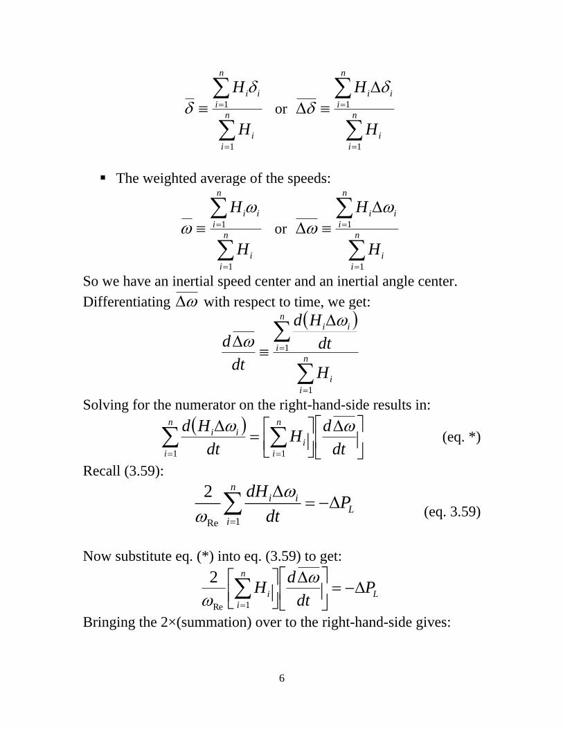
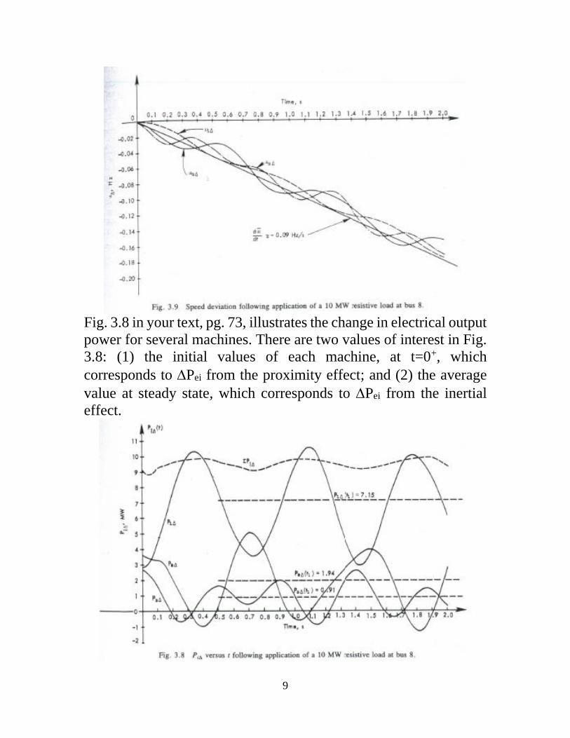
Fig. 3.9 in your text, pg. 75, illustrates the average speed deviation.

9

Fig. 3.8 in your text, pg. 73, illustrates the change in electrical output

power for several machines. There are two values of interest in Fig.

3.8: (1) the initial values of each machine, at t=0+, which

corresponds to Pei from the proximity effect; and (2) the average

value at steady state, which corresponds to Pei from the inertial

effect.

10

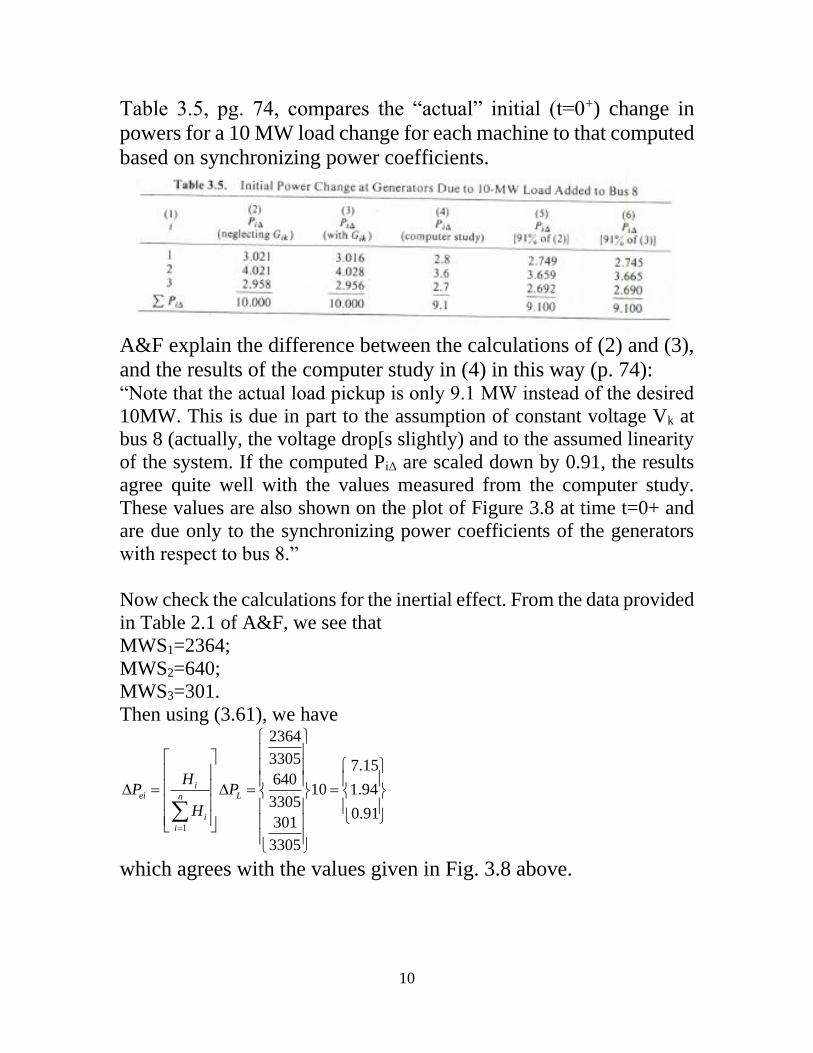
Table 3.5, pg. 74, compares the “actual” initial (t=0+) change in

powers for a 10 MW load change for each machine to that computed

based on synchronizing power coefficients.

A&F explain the difference between the calculations of (2) and (3),

and the results of the computer study in (4) in this way (p. 74): “Note that the actual load pickup is only 9.1 MW instead of the desired

10MW. This is due in part to the assumption of constant voltage Vk at

bus 8 (actually, the voltage drop[s slightly) and to the assumed linearity

of the system. If the computed PiΔ are scaled down by 0.91, the results

agree quite well with the values measured from the computer study.

These values are also shown on the plot of Figure 3.8 at time t=0+ and

are due only to the synchronizing power coefficients of the generators

with respect to bus 8.”

Now check the calculations for the inertial effect. From the data provided

in Table 2.1 of A&F, we see that

MWS1=2364;

MWS2=640;

MWS3=301.

Then using (3.61), we have

1

2364

3305 7.15640

10 1.943305

0.91301

3305

iei Ln

i

i

HP P

H

which agrees with the values given in Fig. 3.8 above.

11

Governor load flow (see Section 2.3.2 in text)

Now what happens when we do model turbine-governors?

From eq. 2.28, we found that, following a load change, the steady-

state change in pu gen mechanical power is related to the steady-

state change in pu frequency according to:

u

u

u

umiu

R

f

RP

where Ru is given in per-unit on the machine base. Typically,

Ru=0.05 in the US (5% droop).

Then we can express that the steady-state change in MW gen

mechanical power is related to the steady-state change in pu

frequency according to:

Bi

u

uBimiumi S

R

fSPP

(**)

Then, relating pu frequency to frequency and substituting into (**)

60

ffu

BiBi

u

mi CSSR

fP

60

So that

Bimi CSP (***)

where

uR

fC

60

Summing over all Pmi yields PL:

L

n

i

Bi

n

i

mi PSCP 11

so that we find:

n

i

Bi

L

S

PC

1

12

Substituting C into eq. (***) above results in:

Ln

i

Bi

Bimi P

S

SP

1

So during the 2-20s period, gens pick up according to their rating.

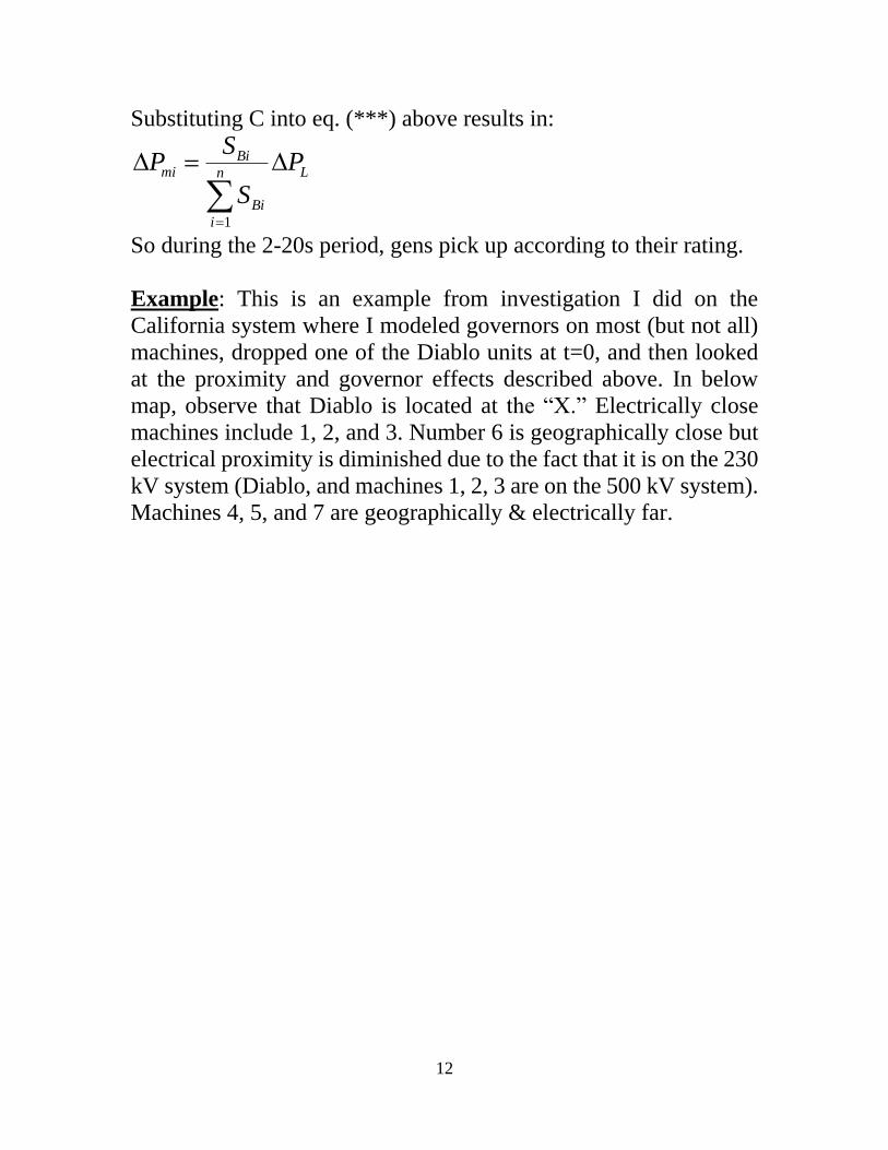
Example: This is an example from investigation I did on the

California system where I modeled governors on most (but not all)

machines, dropped one of the Diablo units at t=0, and then looked

at the proximity and governor effects described above. In below

map, observe that Diablo is located at the “X.” Electrically close

machines include 1, 2, and 3. Number 6 is geographically close but

electrical proximity is diminished due to the fact that it is on the 230

kV system (Diablo, and machines 1, 2, 3 are on the 500 kV system).

Machines 4, 5, and 7 are geographically & electrically far.

13

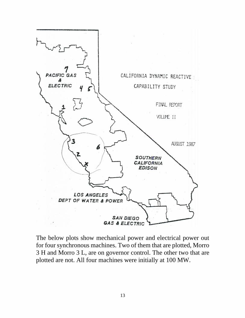
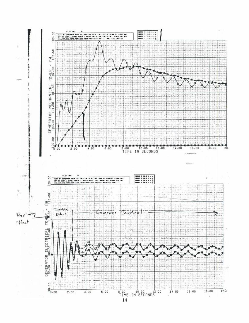
The below plots show mechanical power and electrical power out

for four synchronous machines. Two of them that are plotted, Morro

3 H and Morro 3 L, are on governor control. The other two that are

plotted are not. All four machines were initially at 100 MW.

14

15

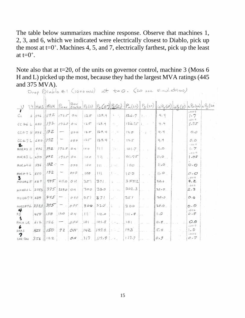
The table below summarizes machine response. Observe that machines 1,

2, 3, and 6, which we indicated were electrically closest to Diablo, pick up

the most at t=0+. Machines 4, 5, and 7, electrically farthest, pick up the least

at t=0+.

Note also that at t=20, of the units on governor control, machine 3 (Moss 6

H and L) picked up the most, because they had the largest MVA ratings (445

and 375 MVA).