1

Summary of Papers

1. P. Sauer and M. Pai, “Power System Steady-State Stability and the Load Flow Jacobian,” IEEETransactions on Power Systems, Vol. 5, No. 4, Nov. 1990

2. V. Ajjarapu and C. Christy, “The Continuation Power Flow: A Tool for Steady-State VoltageStability Analysis,” IEEE Transactions on Power Systems, Vol. 7, No. 1, Feb., 1992.

3. S. Greene, I. Dobson, and F. Alvarado, “Sensitivity of the Loading Margin to Voltage Collapsewith Respect to Arbitrary Parameters,” IEEE Transactions on Power Systems, Vol. 12, No. 1,Feb. 1997, pp. 232-240.

4. S. Greene, I. Dobson, and F. Alvarado, “Contingency Ranking for Voltage Collapse viaSensitivities from a Single Nose Curve,” IEEE Transactions on Power Systems, Vol. 14, No. 1,Feb. 1999, pp. 262-272.

2

Voltage Security

Voltage security is the ability of the system to maintainadequate and controllable voltage levels at all system load buses.The main concern is that voltage levels outside of a specifiedrange can affect the operation of the customer’s loads.

Voltage security may be divided into two main problems:1. Low voltage: voltage level is outside of pre-defined range. 2. Voltage instability: an uncontrolled voltage decline.

You should know that • low voltage does not necessarily imply voltage instability• no low voltage does not necessarily imply voltage stability• voltage instability does necessarily imply low voltage

3

There have been several individuals that have significantlyprogressed the field of voltage security. These include:

• Ajjarapu from ISU

• Van Cutsem: See the book by Van Cutsem and Vournas.

• Alvarado, Dobson, Canizares, & Greene

There are a couple other texts that provide good treatments ofthe subject:• Carson Taylor: “Power System Voltage Stability”• Prabha Kundur: “Power System Stability & Control”

Resources

4

Our treatment of voltage security will proceed as follows:

• Voltage instability in a simple system• Voltage instability in a large system• Brief treatment of bifurcation analysis• Continuation power flow (path following) methods• Sensitivity methods

5

Voltage instability in a simple system

Consider the per-phase equivalent of a very simple threephase power system given below:

Z=R+jX

I

V1V2

S12

Node 1 Node 2

+

__

+

V1 V2

SD=-S21

6

jBGYjXRZ

)sin(||||)cos(||||||

)sin(||||)cos(||||||

212121212

112

212121212

112

GVVBVVBVQ

BVVGVVGVP

121212 jQPS

Let G=0. Then….

)cos(||||||

)sin(||||

21212

112

212112

BVVBVQ

BVVP

Note B>0

7

Now we can get SD=PD+jQD=-(P21+jQ21) by

•- exchanging the 1 and 2 subscripts in the previous equations.•- negating

)cos(||||||

)cos(||||||

)sin(||||

)sin(||||

21212

2

12212

221

2121

122121

BVVBV

BVVBVQQ

BVV

BVVPP

D

D

Define 12 =1- 2

12212

2

1221

cos||||||

sin||||

BVVBVQ

BVVP

D

D

8

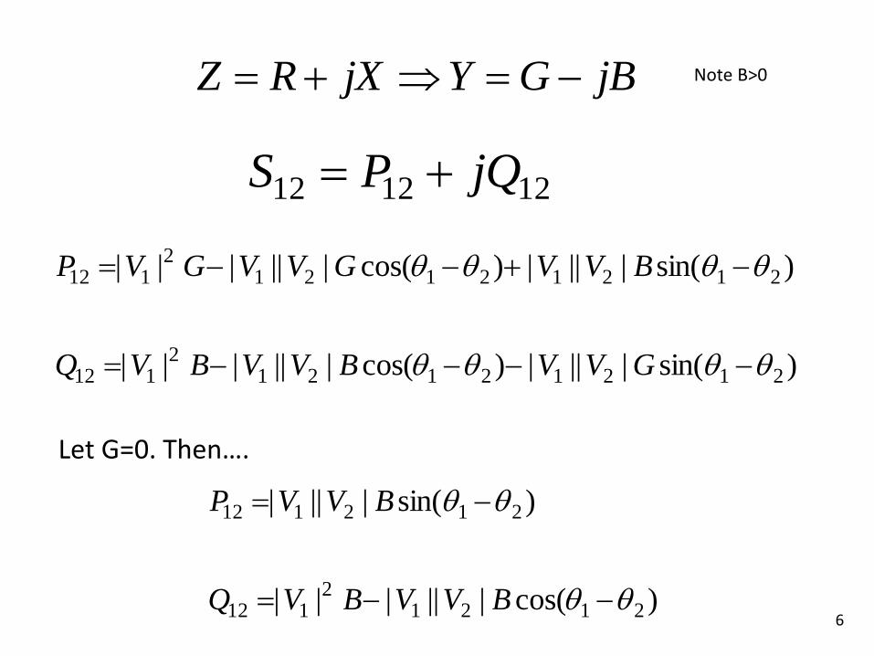
Define: is the power factor angle of the load, i.e.,

IV 2

Then we can also express SD as:

)tan1(

)cos

sin1(cos||||

)sin(cos||||

||||

2

2

2

*

2

jP

jIV

jIV

eIVIVS

D

j

D

Define β=tan. Then

)1( jPjQPS DDDD

Note that phi, andtherefore beta, is positive for lagging,negative for leading.

With V2 phasor as ref,phi is the negative of thecurrent angle and therefore ejphi expressesthe current conjugate.

9

So we have developed the following equations….

12212

2

1221

cos||||||

sin||||

BVVBVQ

BVVP

D

D

)1( jPjQPS DDDD

Equating the expressions for PD and for QD, we have:

1221 sin|||| BVVPD 12212

2

12212

2

cos||||||

cos||||||

BVVBVP

BVVBVPQ

D

DD

Square both equations …..

and add them to get…..

2 2 2 2 2

1 2 12| | | | sinDP V V B 2

2 2 2 2 2

2 1 2 12 | | | | | | cosDP V B V V B

10

222

21

222

2

122

12222

22

122

22

||||)||(

)cos(sin||||)||(

BVVBVPP

BVVBVPP

DD

DD

Gathering terms in (|V2|2)2 and |V2|2 yields:

01||||2

|| 2

2

22

22

1

222

B

PVV

B

PV DD

Note that this is a quadratic in |V2|2. As such, it has the solution:

2/1

21

41

212

2 ||4

||

2

||||

V

B

P

B

PV

B

PVV DDD

11

Let’s assume that the sending end voltage is |V1|=1.0 puand B=2 pu. Then our previous equation becomes:

2

)2(11||

2/12

2

DDD PPP

V

You can makethe P-V plot usingthe followingmatlab code.

% pf = 0.97 laggingbeta=0.25pdn=[0 0.1 0.2 0.3 0.4 0.5 0.6 0.7 0.78];v2n=sqrt((1-beta.*pdn - sqrt(1-pdn.*(pdn+2*beta)))/2);pdp=[0.78 0.7 0.6 0.5 0.4 0.3 0.2 0.1 0];v2p=sqrt((1-beta.*pdp + sqrt(1-pdp.*(pdp+2*beta)))/2);pd1=[pdn pdp];v21=[v2n v2p];% pf = 1.0beta=0pdn=[0 0.1 0.2 0.3 0.4 0.5 0.6 0.7 0.8 0.9 0.99];v2n=sqrt((1-beta.*pdn - sqrt(1-pdn.*(pdn+2*beta)))/2);pdp=[0.99 0.9 0.7 0.6 0.5 0.4 0.3 0.2 0.1 0];v2p=sqrt((1-beta.*pdp + sqrt(1-pdp.*(pdp+2*beta)))/2);pd2=[pdn pdp];v22=[v2n v2p];% pf = .97 leadingbeta=-0.25pdn=[0 0.1 0.2 0.3 0.4 0.5 0.6 0.7 0.8 0.9 1.0 1.1 1.2 1.3];v2n=sqrt((1-beta.*pdn - sqrt(1-pdn.*(pdn+2*beta)))/2);pdp=[1.3 1.2 1.1 1.0 0.9 0.7 0.6 0.5 0.4 0.3 0.2 0.1 0];v2p=sqrt((1-beta.*pdp + sqrt(1-pdp.*(pdp+2*beta)))/2);pd3=[pdn pdp];v23=[v2n v2p];

plot(pd1,v21,pd2,v22,pd3,v23)

12

Plots of the previous equation for different power factors

Real power loading, PD

|V2|

13

Some comments regarding the PV curves:1. Each curve has a maximum load. This value is typically called the maximum system load or the system loadability.2. If the load is increased beyond the loadability, the voltages will

decline uncontrollably.3. For a value of load below the loadability, there are two

voltage solutions. The upper one corresponds to one that can bereached in practice. The lower one is correct mathematically, but Ido not know of a way to reach these points in practice.

4. In the lagging or unity power factor condition, it is clear that thevoltage decreases as the load power increases until the loadability.In this case, the voltage instability phenomena is detectable, i.e., operator will be aware that voltages are declining before the loadability is exceeded.

5. In the leading case, one observes that the voltage is flat, or perhapseven increasing a little, until just before the loadability. Thus, in the leading condition, voltage instability is not very detectable. The leading condition occurs during high transfer conditions when theload is light or when the load is highly compensated.

14

QV Curves

12212

2

1221

cos||||||

sin||||

BVVBVQ

BVVP

D

D

We consider our simple (lossless) system again, with the equations

Now, again assume that V1=1.0, and for a given value of PD

and V2, compute 12 from the first equation, and then QD from thesecond equation. Repeat for various values of V2 to obtain a QVcurve for the specified real load PD.

v1=1.0;b=1.0;

pd1=0.1v2=[1.1,1.05,1.0,.95,.90,.85,.80,.75,.70,.65,.60,.55,.50,.45,.40,.35,.30,.25,.20,.15];sintheta=pd1./(b*v1.*v2);theta=asin(sintheta);qd1=-v2.^2*b+v1*b*v2.*cos(theta);

plot(qd1,v2);

You can make the P-V plot using the following matlab code.

The curve on the next page illustrates….

15

Q-V Curve

QD

|V2|

16

Homework, Homework #1, EE 554, Spring 2018, Dr. McCalley, Due Wednesday, 1/17/2018.

1. Draw the PV-curve for the following cases, and for each, determine the loadability.

a. B=2, |V1|=1.0, pf=0.97 lagging

b. B=2, |V1|=1.0, pf=0.95 lagging

c. B=2, |V1|=1.06, pf=0.97 lagging

d. B=10, |V1|=1.0, pf=0.97 lagging

Identify the effect on loadability of power factor, sending-end voltage, and line reactance.

2. Draw the QV-curves for the following cases, and for each, determine the maximum QD.

a. B=1, |V1|=1.0, PD=0.1

b. B=1, |V1|=1.0, PD=0.2

c. B=1, |V1|=1.06, PD=0.1

d. B=2, |V1|=1.0, PD=0.1

Identify the effect on maximum QD of real power demand, sending-end voltage, and line reactance.

17

Some comments regarding the QV Curves

• In practice, these curves may be drawn with a power flow programby

1. modeling at the target bus a synchronous condenser (a generator with P=0) having very wide reactive limits

2. Setting |V| to a desired value3. Solving the power flow.4. Reading the Q of the generator.5. Repeat 2-4 for a range of voltages.

• QV curves have one advantage over PV curves:They are easier to obtain if you only have a power flow (standard

power flows will not solve near or below the “nose” of PV curvesbut they will solve completely around the “nose” of QV curves.)

18

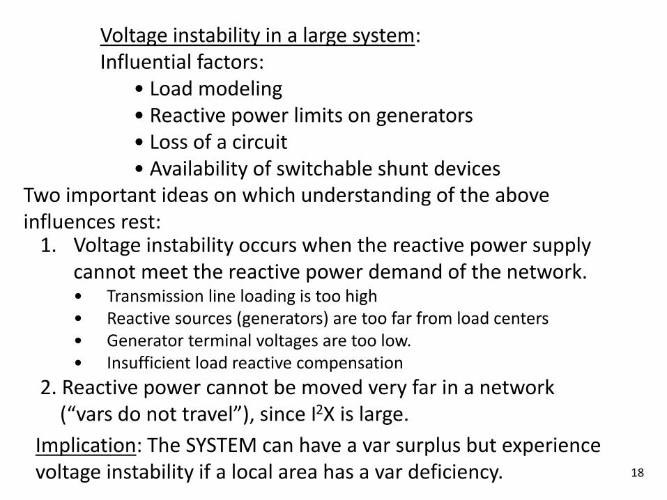
Voltage instability in a large system:Influential factors:

• Load modeling• Reactive power limits on generators• Loss of a circuit• Availability of switchable shunt devices

1. Voltage instability occurs when the reactive power supply cannot meet the reactive power demand of the network.• Transmission line loading is too high• Reactive sources (generators) are too far from load centers• Generator terminal voltages are too low.• Insufficient load reactive compensation

2. Reactive power cannot be moved very far in a network(“vars do not travel”), since I2X is large.

Two important ideas on which understanding of the above influences rest:

Implication: The SYSTEM can have a var surplus but experiencevoltage instability if a local area has a var deficiency.

19

Load modeling

In analyzing voltage instability, it is necessary to consider the networkunder various voltage profiles.

Voltage stability depends on the level of current drawn by the loads.

The level of current drawn by the loads can depend on the voltage seenby the loads.

Therefore, voltage instability analysis requires a model of how theload responds to load variations.

Thus, load modeling is very influential in voltage instability analysis.

20

Exponential load model

A typical load model for a load at a bus is the exponential model:

0

0

0

0 V

VQQ

V

VPP

where the subscript 0 indicates the initial operating conditions.

The exponents and are specific to the type of load, e.g.,

Incandescent lamps 1.54 -Room air conditioner 0.50 2.5Furnace fan 0.08 1.6Battery charger 2.59 4.06Electronic compact florescent 1.0 0.40Conventional florescent 2.07 3.21

21

Polynomial load modelThe ZIP or polynomial model is a special case of the more general exponential model, given by a sum of 3 exponential models with specified subscripts:

3

0

2

2

0

103

0

2

2

0

10 qV

Vq

V

VqQQp

V

Vp

V

VpPP

where again the subscript 0 indicates the initial operating conditions.

0.1321 ppp

So this model is composed of three components:

• constant impedance component (p1, q1) - lighting• constant current component (p2, q2) – motor/lighting• constant power component (p3,, q3) – loads served by LTCs

0.1321 qqq

Usually, values p2 and q2 are the largest.

22

Understanding the effect of each component on voltage instability depends on understanding two ideas:

1. Voltage instability is alleviated when the demand reduces. This is because I reduces and I2X reactive losses in the circuits reduce.

2. Since voltage instability causes voltage decline, alleviation ofvoltage instability results if demand reduces with voltage decline.This gives the key to understanding the effect of load modeling.

• constant impedance load (p1) is GOOD since demandreduces with square of voltage.

• constant current load (p2) is OK since demand reduceswith voltage.

• Constant power load (p3) is BAD since demand doesnot change as voltage declines.

Effect of Load modeling

23

The effects of voltage variation on loads, and thus of loads on voltage instability, cannot be fully captured using exponential orpolynomial load models because of the following three aspects.

• Thermostatic load recovery • Induction motor stalling/tripping• Load tap changers

Some considerations in load modeling

24

Heating load is the most common type of thermostatic load, and it is one for which we are all quite familiar. Although much heating is done with natural gas as the primary fuel, some heating is done electrically, and even gas heating systems always contain some electric components as well, e.g., the fans.

Other thermostatic loads include space heaters/coolers, water heaters, and refrigerators.

When voltage drops, thermostatic loads initially decrease in power consumption. But after voltages remain low for a few minutes, the load regulation devices (thermostats) will start the loads or will maintain them for longer periods so that more of them are on at the same time. This is referred to as thermostatic load recovery, and it tends to exacerbate voltage problems at the high voltage level.

Thermostatic load recovery

25

Three phase induction motors comprise a significant portion of the total load and so its response to voltage variation is important,especially since it has a rather unique response.

Consider the steady-state induction motor per-phase equivalent model.

Induction motor stalling/tripping

Za=R1+jX1

Zb=

Rc//jXm

X’2

R’2+R’2(1-s)/s

=R’2 / s

V1

I’2

26

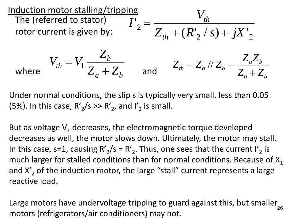
The (referred to stator)rotor current is given by:

Induction motor stalling/tripping

22

2')/'(

'jXsRZ

VI

th

th

whereba

bth

ZZ

ZVV

1

andba

babath

ZZ

ZZZZZ

//

Under normal conditions, the slip s is typically very small, less than 0.05 (5%). In this case, R’2/s >> R’2, and I’2 is small.

But as voltage V1 decreases, the electromagnetic torque developed decreases as well, the motor slows down. Ultimately, the motor may stall. In this case, s=1, causing R’2/s = R’2. Thus, one sees that the current I’2 is much larger for stalled conditions than for normal conditions. Because of X1

and X’2 of the induction motor, the large “stall” current represents a large reactive load.

Large motors have undervoltage tripping to guard against this, but smaller motors (refrigerators/air conditioners) may not.

27

Induction motor stalling/tripping

This phenomena has been called “Fault-induced delayed

voltage recovery” or FIDVR, where

• a three-phase fault depresses voltages

• voltages start to recover but induction motors stall

(particularly single-φ air conditioner compressor motors)

• currents increase (up to 5-6 times); two things happen:

reactive power requirements of local generation

increases, risk of local gen trip increases

voltages remain depressed or recover more slowly

• And then either

Lost generation causes major outage scenario or

voltages increase and restart

28

Induction motor stalling/tripping

Load Shedding Schemes ZIP Load Aggr.

Large 3- Motor Aggr.

Medium 3- Motor Aggr.

Small 3- Motor Aggr.

All 1- Motors Aggr.

Exponential Load Aggr.

To model this, the industry has recently created the composite

load model. It enables modeling load as a composition of

• ZIP

• Four different types of motors, including single-phase

• Electronic load

• Distributed PV

all at the end of a simple one-segment feeder.

“WECC Composite Load

Model (CMPLDW)

Specifications,” January 27,

2015, available at

www.wecc.biz/Reliability/

WECC%20Composite%20

Load%20Model%20Specifi

cations%2001-27-

2015.docx.

29

Induction motor stalling/tripping

cmpldwg 1234 "XXXX" 115.00 "1" : #1 mva=-1.1 /

"Bss" 0 "Rfdr" 0.04 "Xfdr" 0.04 "Fb" 0.75/

"Xxf" 0.08 "TfixHS" 1 "TfixLS" 1 "LTC" 0 "Tmin" 0.9 "Tmax" 1.1 "step" 0.00625 /

"Vmin" 1.025 "Vmax" 1.04 "Tdel" 30 "Ttap" 5 "Rcomp" 0 "Xcomp" 0 /

"Fma" 0.146246 "Fmb" 0.147222 "Fmc" 0.036521 "Fmd" 0.367004 "Fel" 0.106286 /

"PFel" 1 "Vd1" 0.7 "Vd2" 0.5 "Frcel" 0.8 /

"Pfs" -0.99771 "P1e" 2 "P1c" 0.557361 "P2e" 1 "P2c" 0.442639 "Pfreq" 0 /

"Q1e" 2 "Q1c" -0.5 "Q2e" 1 "Q2c" 1.5 "Qfreq" -1 /

"MtpA" 3 "MtpB" 3 "MtpC" 3 "MtpD" 1 /

"LfmA" 0.75 "RsA" 0.04 "LsA" 1.8 "LpA" 0.12 "LppA" 0.104 /

"TpoA" 0.095 "TppoA" 0.0021 "HA" 0.1 "etrqA" 0 /

"Vtr1A" 0.7 "Ttr1A" 0.02 "Ftr1A" 0.2 "Vrc1A" 1 "Trc1A" 99999 /

"Vtr2A" 0.5 "Ttr2A" 0.02 "Ftr2A" 0.7 "Vrc2A" 0.7 "Trc2A" 0.1 /

"LfmB" 0.75 "RsB" 0.03 "LsB" 1.8 "LpB" 0.19 "LppB" 0.14 /

"TpoB" 0.2 "TppoB" 0.0026 "HB" 0.5 "etrqB" 2 /

"Vtr1B" 0.6 "Ttr1B" 0.02 "Ftr1B" 0.2 "Vrc1B" 0.75 "Trc1B" 0.05 /

"Vtr2B" 0.5 "Ttr2B" 0.02 "Ftr2B" 0.3 "Vrc2B" 0.65 "Trc2B" 0.05 /

"LfmC" 0.75 "RsC" 0.03 "LsC" 1.8 "LpC" 0.19 "LppC" 0.14 /

"TpoC" 0.2 "TppoC" 0.0026 "HC" 0.1 "etrqc" 2 /

"Vtr1C" 0.65 "Ttr1C" 0.02 "Ftr1C" 0.2 "Vrc1C" 1 "Trc1C" 9999 /

"Vtr2C" 0.5 "Ttr2C" 0.02 "Ftr2C" 0.3 "Vrc2C" 0.65 "Trc2C" 0.1 /

"LfmD" 1 "CompPF" 0.98 /

"Vstall" 0.56 "Rstall" 0.1 "Xstall" 0.1 "Tstall" 0.03 /

"Frst" 0.2 "Vrst" 0.95 "Trst" 0.3 /

"fuvr" 0.1 "vtr1" 0.6 "ttr1" 0.02 "vtr2" 1 "ttr2" 9999 /

"Vc1off" 0.5 "Vc2off" 0.4 "Vc1on" 0.6 "Vc2on" 0.5 /

"Tth" 15 "Th1t" 0.7 "Th2t" 1.9 "tv" 0.025 /

“DGtype” 1 “pflgdg” 0 “Pgdg” 0.20 “Pfdg” 1.0 “Imax” 1.1 /

“Vt0” 0.6 “Vt1” 0.8 “Vt2” 1.1 “Vt3” 1.2 “Vrec” 0.5 /

“ft0” 58.0 “ft1” 59.0 “ft2” 61.0 “ft3” 62.0 “frec” 0.0

Percentages of motors A, B,

C, D, Electronic

Motor A data

Motor B data

Motor C data

Motor D data

ZIP data

D-PV data

30

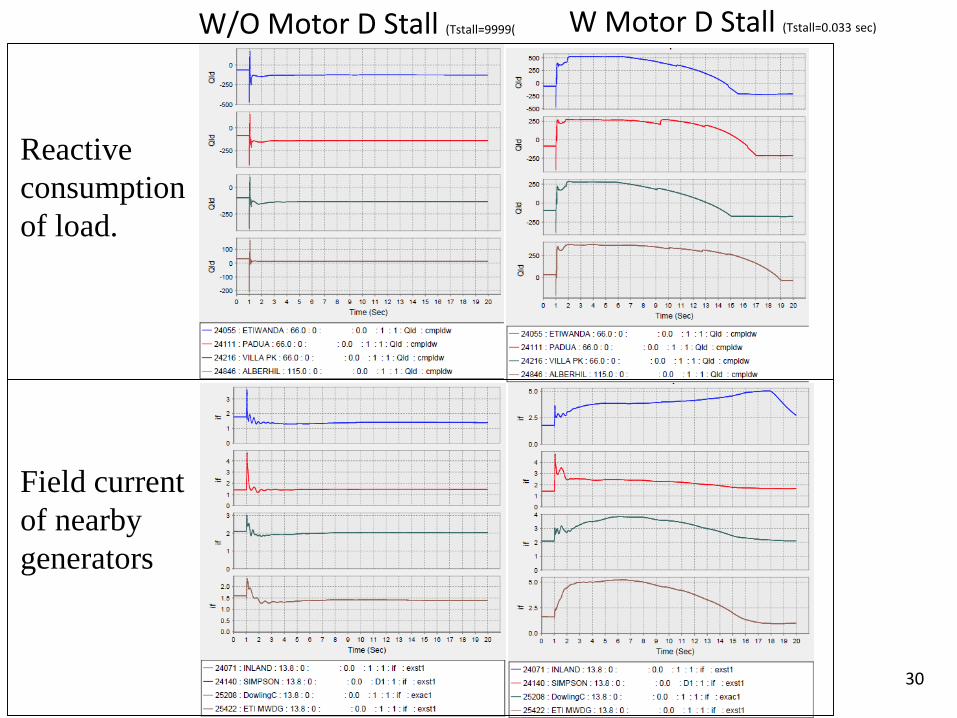
W/O Motor D Stall (Tstall=9999( W Motor D Stall (Tstall=0.033 sec)

Reactive

consumption

of load.

Field current

of nearby

generators

31

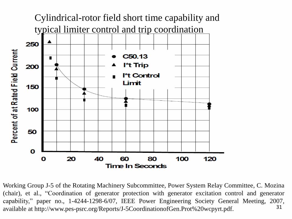
Working Group J-5 of the Rotating Machinery Subcommittee, Power System Relay Committee, C. Mozina

(chair), et al., “Coordination of generator protection with generator excitation control and generator

capability,” paper no., 1-4244-1298-6/07, IEEE Power Engineering Society General Meeting, 2007,

available at http://www.pes-psrc.org/Reports/J-5CoordinationofGen.Prot%20wcpyrt.pdf.

Cylindrical-rotor field short time capability and

typical limiter control and trip coordination

32

Tap changers:

Load tap changers (LTC, OLTC, ULTC, TCUL) are transformers thatconnect the transmission or subtransmission systems to the distributionsystems. They are typically equipped with regulation capability that allow them to control the voltage on the low side so that voltage deviation on the high side is not seen on the low side.

V1V1/t

In per unit, we say that the tap is t:1, where • t may range from 0.85-1.15 pu• a single step may be about 0.005 pu (5/8%=0.00625 is very common)• a change of one step typically requires about 5 seconds.• there is a deadband of 2-3 times the tap step to prevent excessive tap change.

t:1HV side

LV side

V1 and t are given in pu.

Under low voltage conditions at the high side, the LTC will decrease tin order to try and increase V1/t.

33

Tap changers:

Thus, as long as the LTC is regulating (not at a limit), a voltage decline on the high side does not result in voltage decline at the load, in the steady-state, so that even if the load is constant Z,it appears to the high side as if it is constant power. So a simpleload model for voltage instability analysis, for systems using LTC,is constant power!

There are 2 qualifications to using such a simple model (constant power):1. “Fast” voltage dips are seen at the low side (since LTCaction typically requires minutes), and if the dip is low enough, induction motors may trip, resulting in an immediate decrease inload power. 2. Once the LTC hits its limit (minimum t), then the low sidevoltage begins to decline, and it becomes necessary to modelthe load voltage sensitivity.

34

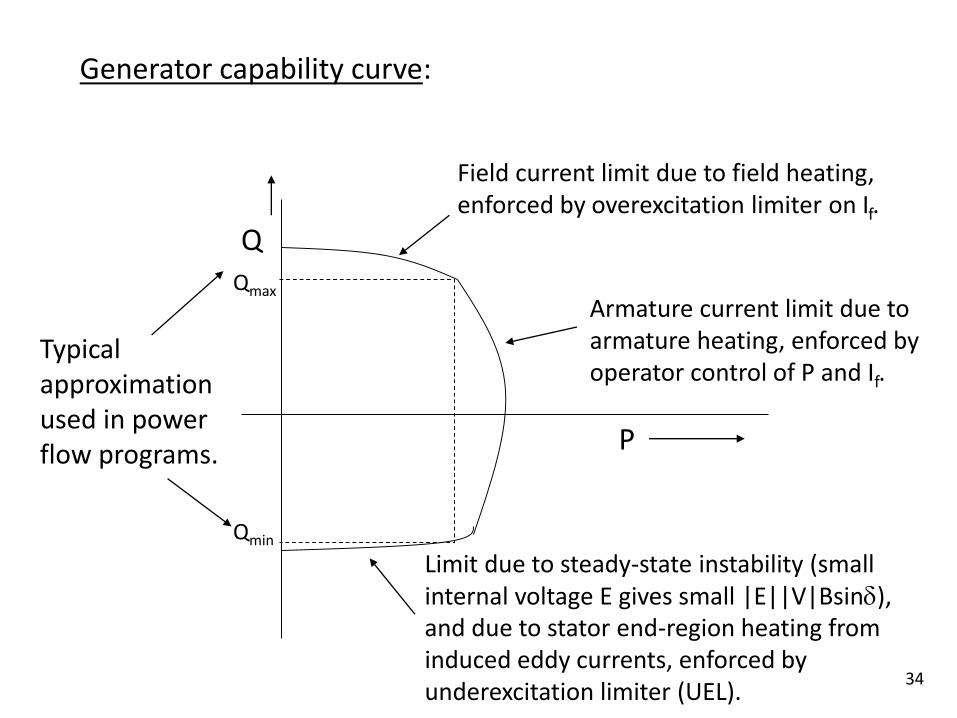
Generator capability curve:

P

Q

Field current limit due to field heating,enforced by overexcitation limiter on If.

Armature current limit due toarmature heating, enforced byoperator control of P and If.

Limit due to steady-state instability (small internal voltage E gives small |E||V|Bsin), and due to stator end-region heating from induced eddy currents, enforced by underexcitation limiter (UEL).

Qmax

Qmin

Typical approximationused in powerflow programs.

35

Effect of generator reactive power limits:

1. Voltage instability is typically preceded by generators hitting their upper reactive limit, so modeling Qmax is very important to analysis of voltage instability.

2. Most power flow programs represent generator Qmax as fixed. However, thisis an approximation, and one that should be recognized. In reality, Qmax is not fixed.The reactive capability diagram shows quite clearly that Qmax is a function of P and becomes more restrictive as P increases. A first-order improvement to fixed Qmax

is to model Qmax as a function of P. 3. Qmax is set according to the Over-eXcitation Limiter (OXL). The field circuit has a

rated steady-state field current If-max, set by field circuit heating limitations. Since heating is proportional to , we see that smaller overloads can be tolerated for longer times. Therefore, most modern OXLs are set with a time-inverse characteristic:

4. As soon as the OXL acts to limit If, then nofurther increase in reactive power is possible.When drawing PV or QV curves, the action of a generator hitting Qmax, will manifest itself as a sharp discontinuity in the curve.

timeoverload

2dtI f

Overload time (sec)

If

Irated

1.0

2.0

120

10

OXL characteristic

36

P

(demand)

|V|

No reactive limits modeled

One generator hits reactive limit

o

Note: Georgia Power Co. models its loadabilitylimit at point x, not point o.

Effect of OXL action on PV curve:

37

Loss of a circuit

I/2

I/2

I

P P

Compare reactive losses with and without second circuit

Qloss=(I/2)2X+ (I/2)2X=I2X/2

Assume both circuits have reactance of X.

Qloss=I2X

Implication: Loss of a circuit will always increase reactive lossesin the network. This effect is compounded by the factthat losing a circuit also means losing its line chargingcapacitance.

X

X

38

Kundur, on pp. 979-990, has an excellent example which illustratesmany of the aforementioned effects. The illustration was done usinga long-term time domain simulation program (Eurostag).

39

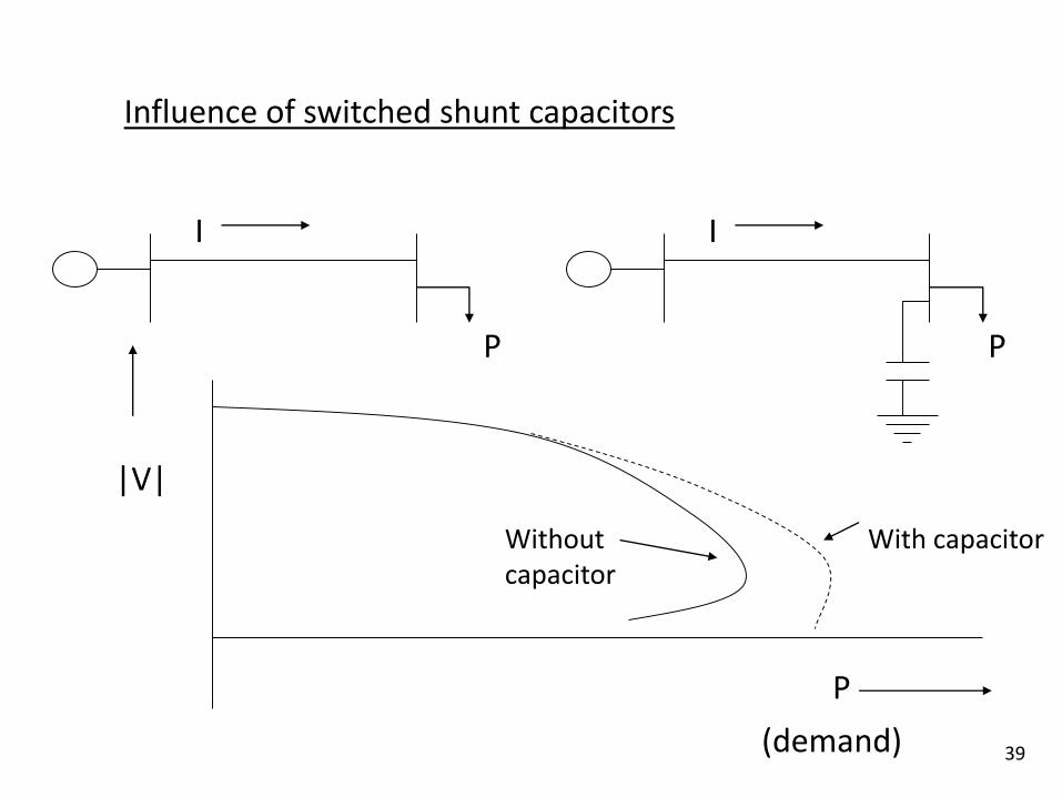
Influence of switched shunt capacitors

I

P

I

P

P

(demand)

|V|

With capacitorWithout capacitor

40

But, shunt compensation has some drawbacks:

• It produces reactive power in proportion to the square of thethe voltage, therefore when voltages drop, so does the reactivepower supplied by the capacitor.

• It has a maximum compensation level beyond which stableoperation is not possible (See pg. 972 of Kundur, and next slide).

(A synchronous condenser and an SVC do not have these 2 drawbacks)

• It results in a flatter PV curve and therefore makes voltage instability less detectable. Therefore, as the load grows in areaslacking generation, more and more shunt compensation is used to keep voltages in normal operating ranges. By so doing, normaloperating points progressively approach loadability.

41

2004006008001000120014001600

Capacitive Mvars

0.6

0.8

1.0

1.2

|V2|

V1=1.0 V2

PL

QL=0

QV-curves drawn

using synchronous

condensor approach.

300 Mvar450 Mvar675 Mvar

950 Mvar

Each QV curve/Capacitor characteristic intersection shows the operating point. Note that for the first three operating points, a small increase in Q-comp (indicated by arrows) results in voltage increase, but for the last operating point (950), more Q-comp (say 960) results in a voltage decrease.S=|V2|2B*Sbase

with |V2|=1.0

42

Bifurcation analysis (ref: A. Gaponov-Grekhov, “Nonlinearities in action” and

also Van Cutsem & Vournas, “Voltage stability of electric power systems.”)

Consider representing the dynamics of the power system as:

),,(0

),,(

pyxG

pyxFx

A differential-algebraic system (DAS): Here x represents state variables of the system (e.g., rotor angles, rotorspeed, etc), y represents the algebraic variables (bus voltage magnitudes & voltage angles), and p represents the real and reactive power injections at each bus. The function F represents the differential equations for the generators, and the function G represents the power flow equations.

A bifurcation, for a dynamic system, is an acquisition of a new quality by the motion of the dynamic system, caused by small changes in its parameters. A power system that has experienced a bifurcation will generally have corresponding motion that is undesirable.

Eqts. 1

43

There are at least two types of bifurcation:• Hopf: two eigenvalues become purely imaginary crossing into the right-half-plane: a birth of oscillatory or periodic motion.• Saddle node: a disappearance of an equilibrium state by virtueof the occurrence of a real eigenvalue at the origin, i.e., azero eigenvalue. A stable operating equilibrium coalesces with an unstable equilibrium and disappears. The dynamic consequence of a generic saddle node bifurcation is a monotonic decline in system variables.

Research activities have concluded that it is the saddle node bifurcation that causes voltage instability.

Types of bifurcations

Im

Re

Im

Re

Hopf Saddle node

44

The Jacobian matrix of eqts. 1:

Y

Y

X

X

G

F

G

FJ

The unreduced Jacobian

and it is referred to as the unreduced Jacobian of the DAS, where

y

xJ

x

0

Eqt. 2

),,(0

),,(

pyxG

pyxFx

Eqts. 1

45

Assuming GY is nonsingular, we may reduce eq. 2 by eliminating the variable y

y

x

G

F

G

Fx

Y

Y

X

X

0

The reduced Jacobian:

This means we need to force the top right hand submatrix to 0, which we can do by multiplying the bottom row by -FYGY

-1 and then adding to the top row.

y

x

GG

GGFFx

YX

XYYX0

0

1

This results in: 1

X Y Y Xx F F G G x

so that the reduced Jacobian matrix is a Schur’s complement:

XYYX GGFFA1

46

Implications 2: 1. If GY is nonsingular, then singularity of A implies singularity of J so

that we may analyze eigenvalues of A to ascertain stability.2. The fact that GY may be nonsingular, yet A singular, means that

load flow convergence is not a sufficient condition for voltage stability.

Stability:

Fact 1 : The conditions for a saddle node bifurcation are 1. Equilibrium:

2. Singularity of the unreduced Jacobian det(J)=0 (a 0 eigenvalue, J noninvertible) .

Y

Y

X

X

G

F

G

FJ

Fact 2: From Shur’s determinant formula, the determinant of a Schur’s complement times the determinant of GY gives the determinant of the original matrix: det(J)=det(A)*det(GY), if GY is nonsingular.

Implication 1: The stability of an equilibrium point of the DAS depends on the eigenvalues of the unreduced Jacobian J. The system will experience a SNB as parameter p changes when J has a zero eigenvalue.

0 ( , , )

0 ( , , )

F x y p

G x y p

47

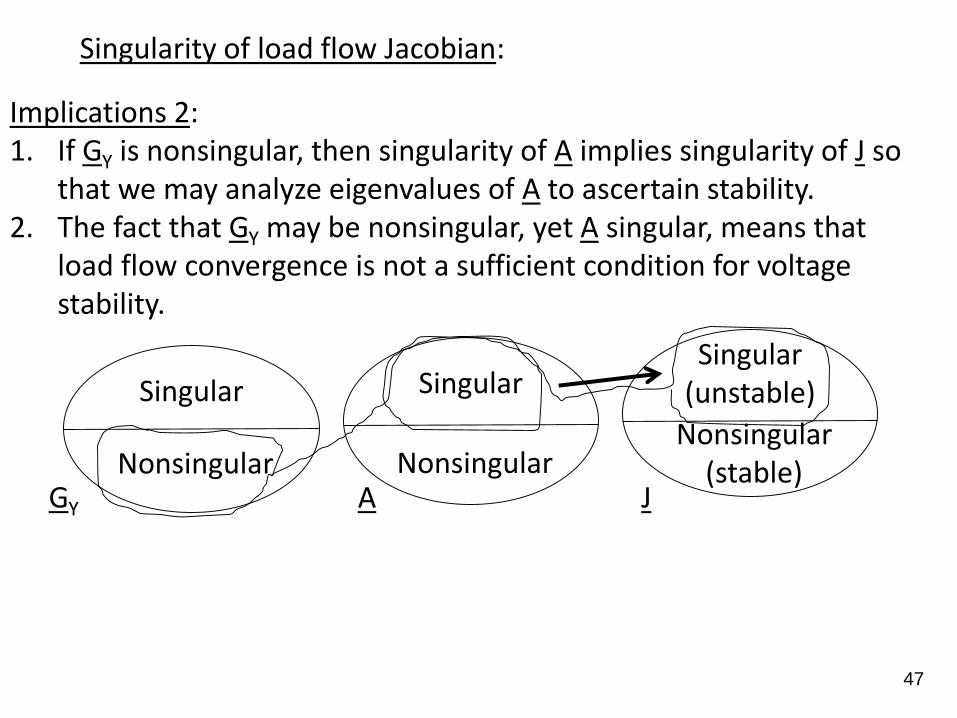
Singularity of load flow Jacobian:

Singular

NonsingularAGY J

Singular

Nonsingular

Singular (unstable)

Nonsingular (stable)

Implications 2: 1. If GY is nonsingular, then singularity of A implies singularity of J so

that we may analyze eigenvalues of A to ascertain stability.2. The fact that GY may be nonsingular, yet A singular, means that

load flow convergence is not a sufficient condition for voltage stability.

48

Singularity of load flow Jacobian:

So voltage instability analysis using only a load flow Jacobian may yield optimistic results when compared to results from analysis of A,that is, stable points (based on Gy) may not be really stable. => However, there is consensus that points identified as unstable using the load flow Jacobian will be really unstable (Schur’s complement does not support that singularity of GY implies singularity of J, however, because it is only valid if GY is nonsingular).

Note: Sauer and Pai, 1990, provide an in-depth analysis of the relationbetween singularity of GY and singularity of J, and show some specialcases for which singularity of GY implies singularity of J (see next slide).

Singular (unstable)

Nonsingular (stable) AGY J

Singular (unstable)

Nonsingular (stable)

Singular (unstable)

Nonsingular (stable)

49

Singularity of load flow Jacobian:

From section 8 of Sauer and Pai’s 1990 paper:

If GY is singular,

then system is

unstable.

If GY is nonsingular,

then system may or

may not be stable.

Non-convergence

may not necessarily

indicate GY

singularity.

50

Singularity of load flow Jacobian:

So, we assume that load flow Jacobian analysis provides an upper bound on stability.

Fact: The bifurcation (zero eigenvalue of GY) of the load flow Jacobian corresponds to the “turn-around point” (i.e., the “nose” point) of a P-V or Q-V curve drawn using a power flow program.

This can be proven using an optimization approach. See pp. 218-220 of the text by Van Cutsem and Vournas.

We have previously denoted the power flow equations as G(x,y,p)=0, but now we denote them as G(y,p)=0, without the dependence on the state variables x (which relate to the machine modeling and include, minimally, and of each machine).

51

So we turn our effort to identifying the saddle node bifurcation(SNB) for the power flow Jacobian matrix.

The Jacobian can reach a SNB in many ways. For example,• increase the impedance in a key tie line• increase the generation level at a generator with weak transmission, while

decreasing generation at all other generators.

• increase the load at a single bus• increase the load at all buses.

In all cases, we are looking for the “nose” point of the V- curve, where is the parameter that is being increased.)

Most applications focus on the last method (increase load at all buses). Key questions here are:• “direction” of increase: are bus loads increased proportionally, or in some other way?• dispatch policy: how do the generators pick up the load increase ?

We will assume proportional load increase with “governor” load flow(generators pick up in proportion to their rating)

|V|

52

|V|

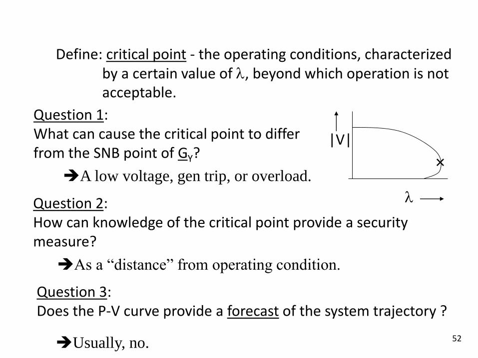
Define: critical point - the operating conditions, characterizedby a certain value of , beyond which operation is notacceptable.

Question 1:What can cause the critical point to differfrom the SNB point of GY?

Question 2:How can knowledge of the critical point provide a security measure?

Question 3:Does the P-V curve provide a forecast of the system trajectory ?

A low voltage, gen trip, or overload.

As a “distance” from operating condition.

Usually, no.

53

Solution approaches to finding *, the value of corresponding to SNB.

Approach 1: Search for * using some iterative search procedure.1. i=12. Using (i), solve power flow using Newton-Raphson.

Here, we iteratively solve G(y,p)=0. At each step,we must solve for y in the eqt: GY y = p

3. If solved, (i+1)= (i)+ .i=i+1go to 2

else if not solved, *= (i+1)

endif4. End

But big problem: as gets close to *, GY becomes ill-conditioned (close to singular). This means that at some point before the criticalpoint, step 2 will no longer be feasible.

54

Approach 2: Use the continuation power flow (CPF).

Predictor step

Corrector step

Pass * ?Select

continuationparameter

Stop

No.

Yes.

55

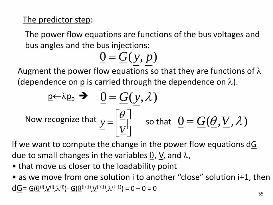
The predictor step:

),(0 pyG

The power flow equations are functions of the bus voltages andbus angles and the bus injections:

Augment the power flow equations so that they are functions of (dependence on p is carried through the dependence on ).

),(0 yG

Now recognize that

Vy

so that ),,(0 VG

If we want to compute the change in the power flow equations dGdue to small changes in the variables , V, and , • that move us closer to the loadability point• as we move from one solution i to another “close” solution i+1, thendG= G((i),V(i),(i))- G((i+1),V(i+1),(i+1)) = 0 – 0 = 0

pp0

56

0

dd

GdVd

Vd

Gdd

d

GdGd

BUT, we have added one unknown, , to the power flow problem without adding acorresponding equation, i.e., in G(,V,)=0, there are are N equations but N+1 variables, so that in eq. 3, the matrix [G GV, G], has N rows (the number of eqts being differentiated) and N+1 columns (the number of variables for which each eqt is differentiated). So we need another equation in order to solve this. What to do ?

Eq. 3

dd

GdVd

Vd

Gdd

d

GdGd

Here, each set of partial derivatives are evaluated at the operating conditions corresponding to the old solution. If the power flow equations are linear with the 3 sets of variables in the region between the old solution and the (close) new one, then their partial derivatives do not change in this region, and so the following is satisfied:

0

d

Vd

d

GGG V

57

The answer to this can be found by identifying how we will be using using the solution to eqt. 3. Note the solution corresponding to the “new” point is:

'

'

'

)(

)(

)(

),1(

),1(

),1(

d

Vd

d

VVi

i

i

pi

pi

pi

If we define to be the “step size,” then we can rewrite this as

d

Vd

d

VVi

i

i

pi

pi

pi

)(

)(

)(

)1(

),1(

),1(

d

Vd

d

d

Vd

d

'

'

'where

Here the “p” indicatesthat this is the “predicted” point.

58

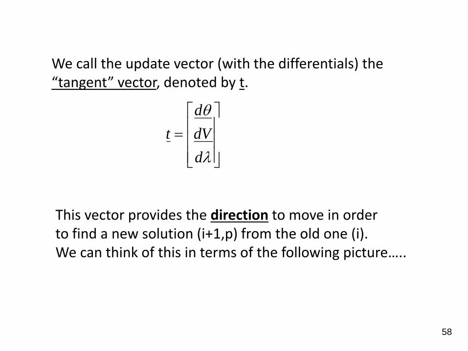
We call the update vector (with the differentials) the “tangent” vector, denoted by t.

This vector provides the direction to move in order to find a new solution (i+1,p) from the old one (i). We can think of this in terms of the following picture…..

d

dV

d

t

59

|V|

Tangent vector

60

So we can set one of the tangent vector elements to be any value we like, then compute the other elements.This provides us with our other equation….

For example, consider a 2-dimensional vector….

Direction= 30o

x1

x2

x2=x1tan(30) so:

- the direction is specified byselecting x1=1, x2=0.5774,

- the direction is specified by selecting x1=0.5, x2=0.2246.

Note: In specifying a direction using an n-dimensional vector, only n-1 of the elements are constrained - one element can be chosen to be any value we like.

61

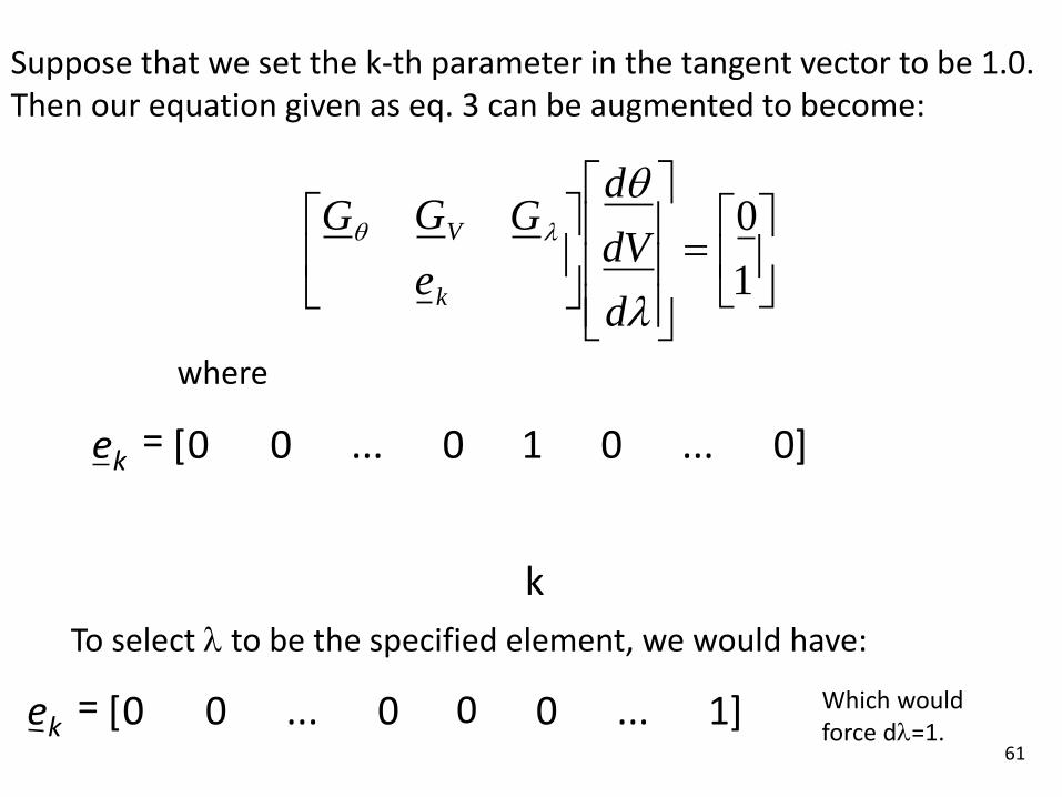
Suppose that we set the k-th parameter in the tangent vector to be 1.0. Then our equation given as eq. 3 can be augmented to become:

1

0

d

dV

dG

e

GG

k

V

where

To select to be the specified element, we would have:

k

]0...010...00[=ke

]1...000...00[=ke Which would

force d=1.

62

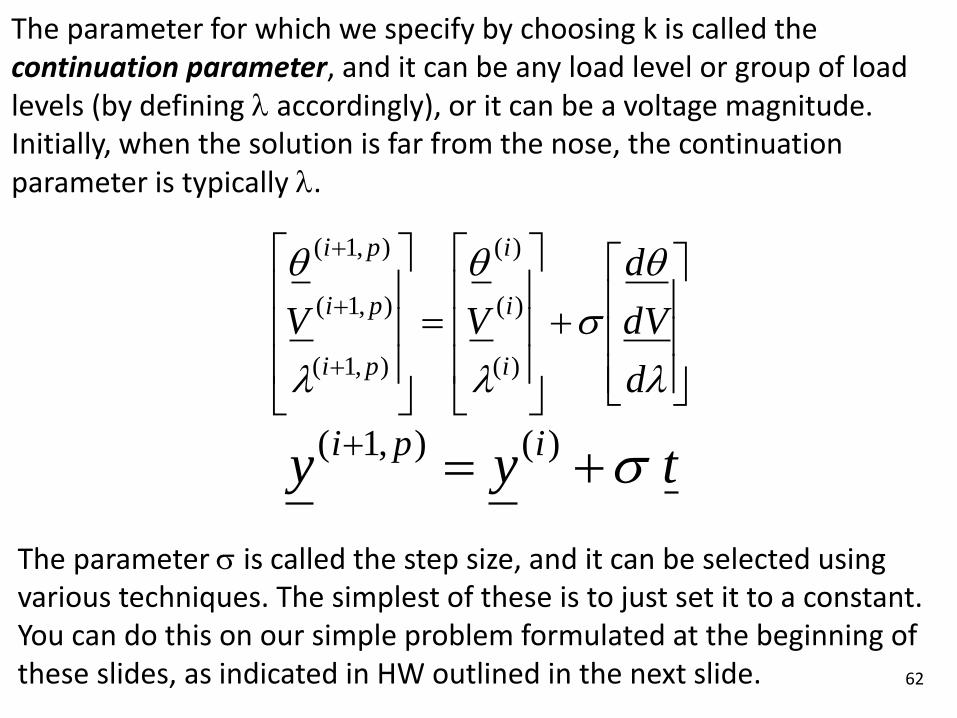
The parameter for which we specify by choosing k is called the continuation parameter, and it can be any load level or group of load levels (by defining accordingly), or it can be a voltage magnitude. Initially, when the solution is far from the nose, the continuation parameter is typically .

d

dV

d

VVi

i

i

pi

pi

pi

)(

)(

)(

),1(

),1(

),1(

The parameter is called the step size, and it can be selected usingvarious techniques. The simplest of these is to just set it to a constant. You can do this on our simple problem formulated at the beginning of these slides, as indicated in HW outlined in the next slide.

tyyipi

)(),1(

63

HOMEWORK #2, Due Wednesday, 1/24.1. Use the equations at the bottom of slide 7.2. Now, just bring the right hand side of these 2 equations over to the

left-hand side, and you have the 2 equations that correspond to G(y,p)=0. 3. Solve these equations to get the corresponding power flow solution (but

you do not need Newton-Raphson to do this – you can just use the equation at the bottom of slide 10). You will get two solutions; use the solution with the higher voltage.

4. Now you need to replace the value specified in the equations for PD (assuming that the initial load is 0.4) with 0.4*lambda. This gives you the equations in the form of slide 55: 0=G(theta,V,lambda).

Note, however, that G is really two equations: G1 and G2.You will need to use V1=1.0, B=2.0, and pf=0.97 lagging.5. Now you need to formulate the equations on the slide 55. This is a matter of taking derivatives and then evaluating those derivatives at the solution that you obtained above. Note, however, the each element in the matrix of slide 61 actually represents 2 elements. That is:

| dG1/dtheta dG1/dV dG1/dlambda|| dG2/dtheta dG2/dV dG2/dlambda|| 0 0 1 |

6. Evaluate each of the above matrix elements at the solution obtained in step 3.7. Then solve these equations for the tangent vector. You can do this by

inverting the above matrix (use matlab or a calculator to do this) and then multiply the right-hand-side by this inverted matrix.

8. Then take a “step” using an appropriately chosen step size per the equation on slide 62.

9. Beginning from your predicted point that you identified in step 8, develop equations for approach a, solve them, and identify the resulting corrected point in terms of voltage and power.10. Repeat #9 except implement approach b.

12212

2

1221

cos||||||

sin||||

BVVBVQ

BVVP

D

D

#9 and #10 will be explained in next few slides. Note to solve these two parts, you will need to perform Newton-Raphson with a chosen solution tolerance.

64

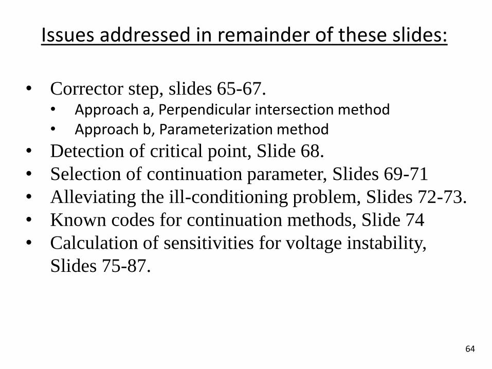
Issues addressed in remainder of these slides:

• Corrector step, slides 65-67.• Approach a, Perpendicular intersection method• Approach b, Parameterization method

• Detection of critical point, Slide 68.

• Selection of continuation parameter, Slides 69-71

• Alleviating the ill-conditioning problem, Slides 72-73.

• Known codes for continuation methods, Slide 74

• Calculation of sensitivities for voltage instability,

Slides 75-87.

65

Note, however, that the predicted point will satisfy thepower flow equations only if the power flow equations arelinear, which they are not. That is, the partial derivatives are not constant in the region between old and new points.

So our point needs correction. This leads to the corrector step.

There are two different approaches for performing thecorrector step.

Approach a: Perpendicular intersection method.

Approach b: Parameterization method

Corrector step

66

Approach a: perpendicular intersection

Here, we find the intersection between the power flowequations (the PV curve) and a plane that is perpendicular (, orthogonal) to the tangent vector.

|V|

0),1()1(

tyypii

t

),(0 )1()1( ii

yG y(i+1)

y(i+1,p)y(i)

Solve simultaneously,for y(i+1)

Use Newton-Raphson to solve the above (requires only 1-3 iterations since we have good starting point). If no convergence, cut step size () by half and repeat.

The last equation says the inner (dot) product of 2 vectors is zero.

y(i+1)-y(i+1,p)

-y(i+1,p)

y(i+1,p)y(i+1)

t

67

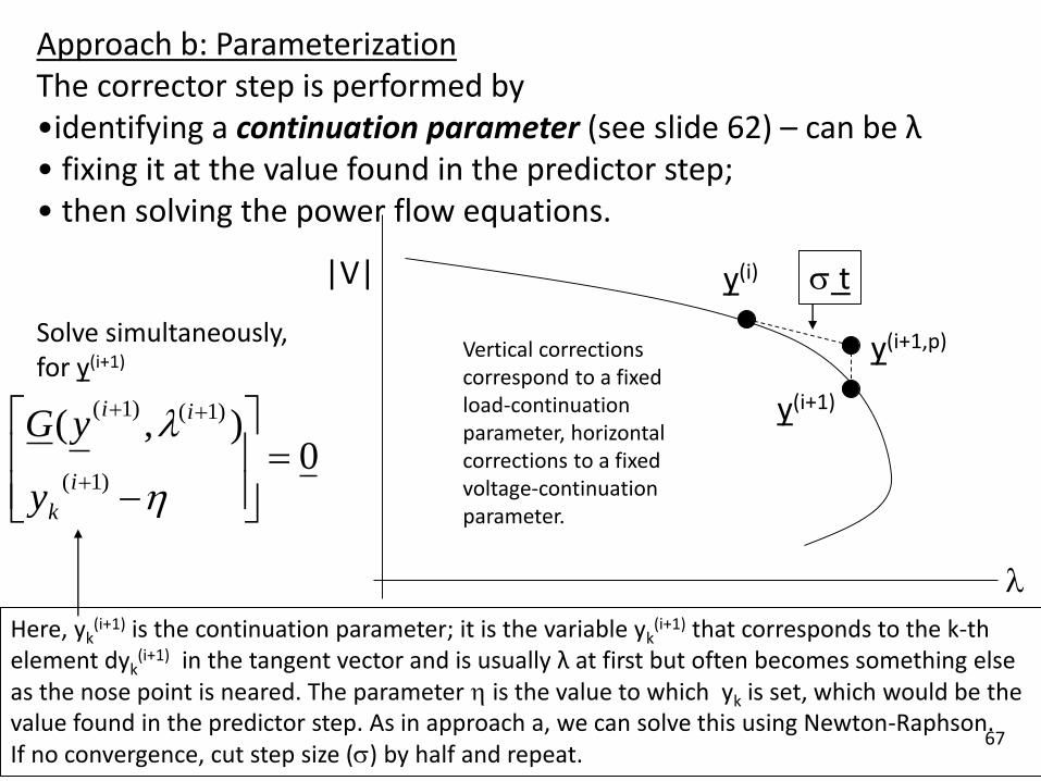
Approach b: ParameterizationThe corrector step is performed by •identifying a continuation parameter (see slide 62) – can be λ• fixing it at the value found in the predictor step;• then solving the power flow equations.

|V|

t

y(i+1)

y(i+1,p)

y(i)

0),(

)1(

)1()1(

i

k

ii

y

yG

Here, yk(i+1) is the continuation parameter; it is the variable yk

(i+1) that corresponds to the k-th element dyk

(i+1) in the tangent vector and is usually λ at first but often becomes something else as the nose point is neared. The parameter is the value to which yk is set, which would be the value found in the predictor step. As in approach a, we can solve this using Newton-Raphson. If no convergence, cut step size () by half and repeat.

Solve simultaneously,for y(i+1)

Vertical correctionscorrespond to a fixedload-continuationparameter, horizontalcorrections to a fixedvoltage-continuation parameter.

68

Detection of critical point:

We will know that we have surpassed the critical point when the sign of d in the tangent vector becomes negative, because it is at this point where the loading reaches a maximum point and begins to decrease.

|V|

x

increasing

decreasing

69

Selection of continuation parameter:

d

dV

d

VVi

i

i

pi

pi

pi

)(

)(

)(

),1(

),1(

),1(

Typically, yk

is going to beone of these.

The continuation parameter is selected from among and the variables in y according to the one that ischanging the most with . This will be the parameter thathas the largest element in the tangent vector. • relatively unstressed conditions (far from nose): generally • relatively stressed conditions (close to nose): generally thevoltage magnitude of the weakest bus, as it changes a great deal as is changed, when we are close to *.

The one changingthe most with λ is most sensitive andrepresents a variable that we want to be carefulwith as we look for another solution, so it makes sense to keep it constant.

70

Selection of continuation parameter (unstressed condition):

|V|

y(i+1)

y(i+1,p)

y(i)

Here, is fixed.

The continuation parameter is selected from among and the state variables in y according to the one that ischanging the most with . This will be the parameter thathas the largest element in the tangent vector. • relatively unstressed conditions (far from nose): generally .=> This looks like below.

71

• relatively stressed conditions (close to nose): generally thevoltage magnitude of the weakest bus. Here, the voltage beingplotted is chosen as the continuation parameter.

|V|

y(i+1)

y(i+1,p)

y(i)

Here, |V| is fixed.

“Essentially, a variable is fixed as a parameter (the voltage), andthe parameter () is treated as a variable. This process of selectinga variable to fix is sometimes called the parameterization step.”

-Scott Greene, Ph.D. dissertation, 1998.

Selection of continuation parameter (stressed condition):

72

A central question:

How does the continuation technique alleviate the ill-conditioning problem experienced by a regular power flow ?

0),1()1(

tyypii

),(0 )1()1( ii

yG 0

)(

)1(

)1()1(

i

k

ii

y

yG

Refer to the solutions procedures for the two corrector approaches.Perpendicular interesectionSolve simultaneously,for y(i+1)

ParameterizationSolve simultaneously,for y(i+1)

In both cases, we use Newton-Raphson to solve, so we need to obtain theJacobian. But the Jacobian is slightly different than in normal power flow.

73

The Jacobian of the power flow equations is just Gy, but the Jacobian of the equations in the two corrector approaches will have an extra row and column.

k

k

x

x

y

y

C

G

C

G

Here, C is the additional equation, and xk is the selectedcontinuation parameter.

This addition of a row and column to the Jacobian has theeffect of improving the conditioning so that the previouslysingular points can in fact be obtained. In other words, theadditional row and column provides that this Jacobian is nonsingular at * where the standard Jacobian is singular.

74

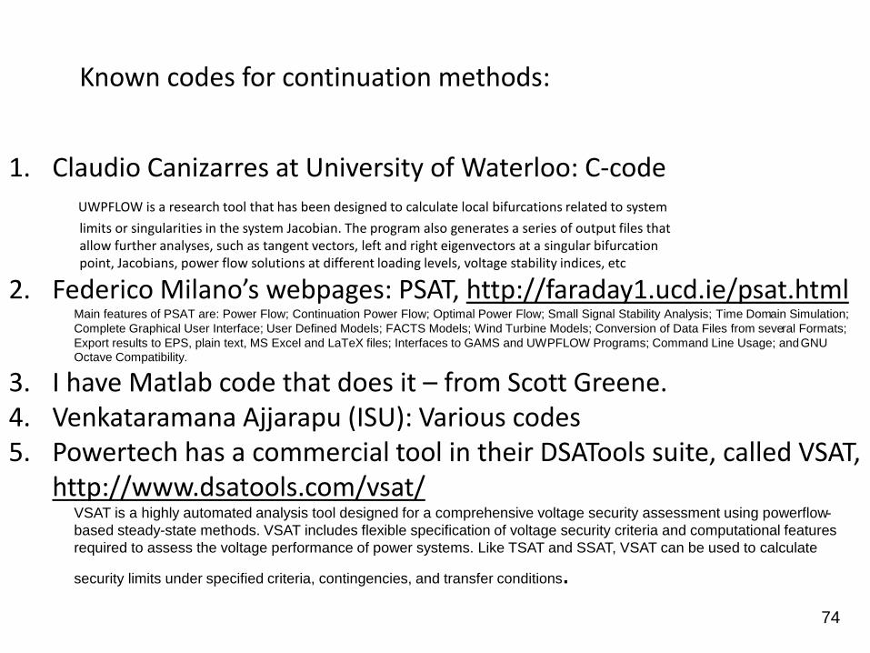
Known codes for continuation methods:

1. Claudio Canizarres at University of Waterloo: C-code UWPFLOW is a research tool that has been designed to calculate local bifurcations related to system

limits or singularities in the system Jacobian. The program also generates a series of output files that allow further analyses, such as tangent vectors, left and right eigenvectors at a singular bifurcation point, Jacobians, power flow solutions at different loading levels, voltage stability indices, etc

2. Federico Milano’s webpages: PSAT, http://faraday1.ucd.ie/psat.htmlMain features of PSAT are: Power Flow; Continuation Power Flow; Optimal Power Flow; Small Signal Stability Analysis; Time Domain Simulation;

Complete Graphical User Interface; User Defined Models; FACTS Models; Wind Turbine Models; Conversion of Data Files from several Formats;

Export results to EPS, plain text, MS Excel and LaTeX files; Interfaces to GAMS and UWPFLOW Programs; Command Line Usage; andGNU

Octave Compatibility.

3. I have Matlab code that does it – from Scott Greene.4. Venkataramana Ajjarapu (ISU): Various codes5. Powertech has a commercial tool in their DSATools suite, called VSAT,

http://www.dsatools.com/vsat/VSAT is a highly automated analysis tool designed for a comprehensive voltage security assessment using powerflow-

based steady-state methods. VSAT includes flexible specification of voltage security criteria and computational features

required to assess the voltage performance of power systems. Like TSAT and SSAT, VSAT can be used to calculate

security limits under specified criteria, contingencies, and transfer conditions.

75

Calculation of sensitivities for voltage instability analysis

What is a sensitivity ?

It is the derivative of an equation with respect to a variable.It shows how parameter 1 changes with parameter 2.

It is: exact when parameter 2 depends linearly on parameter 1.It is approximate when parameter 2 depends nonlinearly on parameter 1,

but it is quite accurate if it is only used close to where it is calculated.

76

Consider the system characterized by G(y). Thenis the sensitivity of the equation G with respect to y,evaluated at y*.

*yy

G

G(y)

yy*

Slope is G/y evaluated at y*.

y

It’s usefulness is that once it is calculated, it can be used to QUICKLY evaluate f(y) from G(y)G(y*)+ (G/y|y*)y,

BUT ONLY AS LONG AS y IS CLOSE TO y*.

y

77

Consider parameter p: we desire to obtain the sensitivity ofG(y,p) to p. Typical parameters p would be a bus load, a buspower factor, or a generation level.

Very important to distinguish between • voltage sensitivities

• voltage instability sensitivities

What is the difference between them in terms of • what they mean ?• how to compute them ?

78

Sensitivities for bus voltage

These we compute at the current operating condition.

For a given continuation parameter, they can be obtainedfrom the first predictor step in the continuation power flow.

|V|

Current operating point

d

dV

d

tRecall that this provides us withthe tangent vector, given by:

The tangent vector is the vector of sensitivities with respect to a smallchange in , so the portion of the vectordesignated as dV is exactly the voltagesensitivities.

79

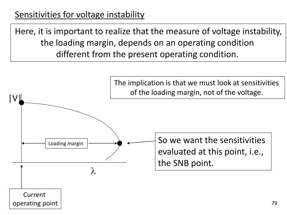
Sensitivities for voltage instability

Here, it is important to realize that the measure of voltage instability,the loading margin, depends on an operating condition

different from the present operating condition.

The implication is that we must look at sensitivities of the loading margin, not of the voltage.

|V|

Current operating point

So we want the sensitivities evaluated at this point, i.e., the SNB point.

Loading margin

80

Let S be the vector of real and reactive load powers,and k be the direction of load increase.

kSS 0

Also, define L as the loading margin (a scalar), so thatthe load powers resulting in the SNB point are given by:

Derivation of loading margin sensitivities at SNB point.

We desire to find the sensitivity of the loading margin L to a change in the parameter p. We denote this sensitivity by Lp.

kSS L0

81

Consider the system characterized by

G(y,S, p) = 0

Assumption: the system has a SNB at (y*,S*, p*), i.e., :

1. G(y*,S*, p*) = 0 (an equilibrium point)

2. Gy(y*,S*, p*) is singular (zero eigenvalue), and

w is a left eigenvector of Gy(y*,S*, p*), corresponding

to the zero eigenvalue so that (by definition of the lefteigenvector)

wT Gy(y*,S*, p*) =0 wT=0

Note that Gy(y*,S*, p*), being singular, cannot be inverted, but

we can compute it (that is, Gy (y*,S*, p*)), and its eigenvectors.

3. wT GS(y*,S*, p*) 0

We want the sensitivity of the loading margin to p.

82

The points (y,S, p) satisfying numbers 1 and 2 correspond to SNB points,

and we can obtain a curve of such points byvarying p about its nominal value p*.

Linearization of this curve about the SNB point results in

0***

pGSGyG pSy

where the notation |* indicates the derivatives are evaluated at the SNB point.

Pre-multiplication by the left eigenvector w results in:

0***

pGwSGwyGw p

T

S

T

y

T

By #2 on the previous slide, the first term in the above is zero. So...

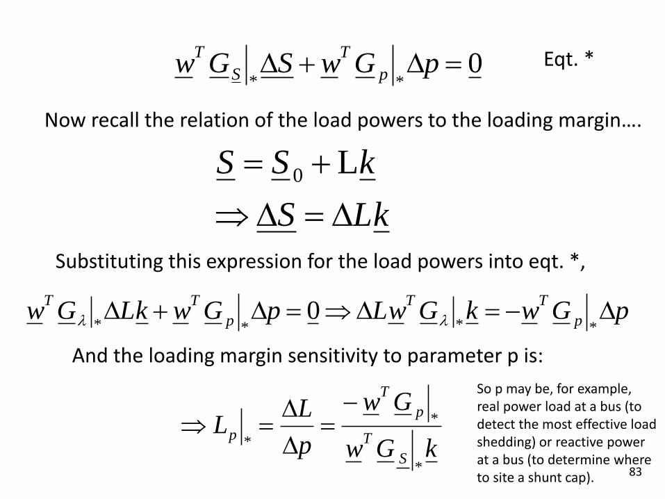
83

0**

pGwSGw p

T

S

T

pGwkGwLpGwkLGw p

TT

p

TT

****0

kLS

kSS

L0

kGw

Gw

p

LL

S

T

p

T

p

*

*

*

Now recall the relation of the load powers to the loading margin….

Substituting this expression for the load powers into eqt. *,

Eqt. *

And the loading margin sensitivity to parameter p is:

So p may be, for example,real power load at a bus (to detect the most effective loadshedding) or reactive power at a bus (to determine where to site a shunt cap).

84

Some comments about computing Lp

• The left eigenvector w must be computed for the Jacobian Gy evaluated at the SNB point.

• You only need to compute w and GS once, independent of how many sensitivities you need. Methods to compute the left eigenvector w include QR or inverse iteration.

• The vector of derivatives with respect to the parameter p, which is Gp, is typically sparse. For example, if you want to compute the sensitivity to a bus power, then there would be only 1 non-zero entry in Gp.

• The matrix of derivatives with respect to the load powers, GS, using constant power load models, is a diagonal matrix with ones in the rows corresponding to load buses. This is because a particular load variable would ONLY occur in the equation corresponding to the bus where it is located, and for these equations, these variables appear linearly with 1 as coefficient.

kGw

GwL

S

T

p

T

p

*

*

*

85

Some comments about extensions

• Multiple sensitivities may be computed using Gp (a matrix) instead of Gp (a vector).

In this case, the result is a vector.

• A sensitivity to a line outage may be obtained by letting p contain elements corresponding to the outaged line parameters.

kGw

GwL

S

T

p

T

p

*

*

*

• Getting multiple sensitivities can be especially attractive when we want to findthe sensitivity to several simultaneous changes. One good example is to find thesensitivity to changes in multiple loads.

• A special case of this is to find the sensitivity to changes at ALL loads, which is very typical, given a particular loading direction k . Then

i

pi iLkL

*loads all

86

Some comments about extensions

• A sensitivity to a line outage may be obtained by letting p contain elements corresponding to the outaged line parameters: R (series conductance), X (seriesreactance), and B (line charging). Then use the multiple parameter approach.

kGw

GwL

S

T

p

T

p

*

*

*

pLL p *

Zpq=R + jX

p q

jBjB

• Here, p = [R X B]T.

• Note that p is NOT SMALL ! Therefore L may have considerable error.For that reason, this one needs to be careful about using this approach to compute the actual loading margins following contingencies.

• However, it certainly can be used for RANKING contingencies. One might consider having a “quick approximation” and a “long exact” risk calculation.

87

• Greene, et al., also propose a quadratic sensitivity which requires calculation of a second order term Lpp . This is used together with the linear sensitivity according to

Some comments about alternatives

• Invariant Subspace Parametic Sensitivity (ISPS) by Ajjarapu.Advantages:

– based on differential-algebraic model– provides sensitivities at ANY point on the P-V curve

2

**

)(2

1pLpLL ppp

It requires significantly more computation but can provide greateraccuracy over a larger range of p.