1

EE 554 PROJECT ASSIGNMENT, SPRING 2020, DR. MCCALLEY

Due: April 30, 2020

Your assignment is to perform an operating study for the Diablo Canyon Nuclear

Power Plant using the power flow and stability data provided to you by the

instructor. The objective of the study is to determine the safe operating limits for

the plant, in terms of MW output power, under the NERC disturbance class P1

given in the NERC Planning Standards. You may assume that this criterion is

condensed to “the system must perform satisfactorily for a three-phase fault at the

machine terminals followed by loss of a single circuit.” To perform satisfactorily,

the machine must be stable and no first-swing transient voltage dip can fall below

0.75 per-unit.

There are three 500 kV lines emanating from the plant under “normal” conditions.

You are to develop the MW operating limits for a “weakened” condition whereby one

line is out on maintenance. Since two of the lines are identical, this means that you

must develop two different operating limits: with lines A, B, C, and A and B identical,

you must identify (1) the operating limit with A out (2) the operating limit with C out.

I expect that everyone will use the Powertech software PSAT (for power flow) and

TSAT (for time-domain simulation). I do not object if you want to use something else,

but I will not be very able to help you with program issues if you do use something

else. The basic commands to access the needed software are as follows:

============================================================= INSTRUCTIONS UPDATED 3/25/2020:

In order to access the VDI pool the directions listed at https://it.ece.iastate.edu/vdi/ may be helpful.

But I suggest you follow the below.

Please note that it is not necessary to login to the ISU VPN at this time.

1. Install Horizon client from https://vlab.ece.iastate.edu (the install required that I restart my machine so be prepared for that).

2. After installing and restarting, click on the “Horizon” tab on your desktop and you will see an icon on the top left hand corner with a “+” in the middle. Click on that, and you will get a request to enter the name of the connection server. To this request, you should enter “vlab.ece.iastate.edu” (without quotes).

3. Then it will ask you to log in. Use your ISU NetID and password. 4. Once logged in, you should see a screen with an icon in the upper left hand corner that says “EE 554.”

Click on this icon and it will load your desktop.

2

5. Hopefully that will do it. But in my case I got a message that said “Windows could not create the shortcut.” I clicked on “OK” and then from “Start” button I found “DSATools” from which I was able to start PSAT and TSAT.

=====================================================================================================

Off-campus students may have access to DSATools via their employer, and if

acceptable to the employer, you may certainly use it that way. If you do not, then you

can use the same procedure as described above, except you will have to connect to the

VPN. Instructions for doing this are at the same URL given above, i.e., they are at

https://it.ece.iastate.edu/vdi/. In brief, connect to vpn.iastate.edu with a web browser,

install cisco any-connect from that site, then connect to cisco any-connect, and then

you are “on campus” thru the vpn.

=============================================================

You are provided (on the website) with 4 data files:

- wecc179.raw: The power flow raw data file in PTI Version 30 format.

- wecc179.dyr: The machine data for all machines in the system.

- Monitor.mon: This specifies the quantities you can inspect via the plotting

routine.

- faultbus103.swi: This specifies the contingency.

These data files are from a test system which is similar in structure to the

transmission system of the western U.S. However, I stress “similar” for two reasons:

1. The system is a product of gross approximation. Many essential features are

omitted in order to keep the system relatively simple and small in terms of number

of buses, lines, and machines. For example, this system represents only 179 buses.

Actual models of the western US grid typically have on the order of 20000 buses.

2. I do not have authority to provide accurate transmission models of the western US

grid.

So one should understand that any results obtained using this model pertain only to

this model and has very little relevance to the actual western US grid.

Two high-level one-line diagrams of the overall system are given in Fig. 1 below, and

Fig. 2 provides a more refined view of the portion of the system to be studied.

3

PA

CI

cal

sw

nw ne

33

32 31

30

35

80

78

74 79

66

75

77

76

72

82 81

86

84

85 156

157

16 1

162

v

v

167 165

158 159

155

44

45 160

166

163

5

11

6

8

9

1 8

17

4

3

7

13 138

147

15

19

112

115

118 119

103

107

108

110

102

104

109

142

37 64

63

56 153

145

151

152

49

48 47

146

154

150

149

143

42

43

141

140

50

57

nw

cal

ne

sw

PACI

Diablo

Canyon

Fig. 1: High-level system one-line

Diablo500

#102

Diablo25.0

#103

Gates500

#104

Midway500

#108

Fig. 2: Lower-level view of study area

You should be aware that there are two identical generating units at Diablo Canyon.

Dynamic data for one of these plants are given below. ********************************************************************************

THE BELOW CONTAINS STABILITY DATA FOR THE POWER PLANT OF INTEREST IN THE STUDY.

NOTE THAT THERE ARE TWO UNITS, BUT I HAVE ONLY PROVIDED DATA FOR ONE UNIT. YOU MAY ASSUME

THAT THE TWO UNITS ARE IDENTICAL. THE CORRSPONDING BUS NUMBER IN YOUR POWER FLOW DATA IS

4

103. THERE IS DATA FOR THIS PLANT IN THE STABILITY DATA FILE FOR YOUR SYSTEM, WHICH IS

CALLED wecc179.dyr. YOU MUST CHECK THE DATA IN THE FILE TO VERIFY THAT THE MACHINE DATA IS

CORRECT IN RELATION TO THE BELOW. IF IT IS NOT, THEN YOU MUST CORRECT IT. YOU NEED NOT BE

CONCERNED ABOUT THE EXCITATION DATA (CARDS FC AND FZ), THE PSS DATA (CARD SF), THE GOVERNOR

DATA (CARD GS), OR THE TURBINE DATA (CARD TB).

********************************************************************************

UT

NY O

IP W

I P TE N X''D X''Q T''DT''Q

MD < NAME ><KV>D<MVA> <F> <#> <> < > < >< >< >< >

MD DIABLO CYN 211340. 90 1 N PG+ 0.2810.281.043.124

--------

I P Q MVA T'D T'Q SG10 SG12 D

MF < NAME ><KV>D<MWS ><%><%>< ><RA><X'D><X'Q><XD ><XQ >< >< ><XL >< >< >< >

MF DIABLO CYN 214650.01.01.0134000210.3460.9911.6931.6366.581.5 2280.07690.410.0

FC DIABLO CYN 21 .0000 0 0 40000 2 6.0 -6.0 1000 15

FZ DIABLO CYN 21 563 390 0 3850 40 10000.000 0

SF DIABLO CYN 21 0 020.00251000 20.322 0 0 0 0 .05 0

GS DIABLO CYN 211208.0 0.05 0.18 0.0 0.04 0.1 0.2

TB DIABLO CYN 210.200 0.30 5.0 0.70 0

However, the data in your system files (power flow and stability) represents only a

single unit at the power plant. I have scanned the system data files and feel that the

data for this plant is questionable. You need to check it to verify that it appropriately

represents a single machine equivalent of the two machines given in the data below.

Specifically, you need to check two things, one in pf data and one in dynamic data.

In what follows, Section A identifies how to modify the power flow data and how to

run the power flow program. Section B identifies how to modify the dynamic data.

Section C identifies how to run the time-domain simulation program.

A. Modifying pf data and running pf program

The power flow data, especially the transformer impedance (the transformer

impedance should be approximately 0.10 pu, when given on the machine base,

but of course it must be converted to the 100 MVA system base when entered in

the data).

Note from the above “MF” card, we observe that the MVA base of the machine is

1340. If we are to represent two identical such machines, then the MVA base will be

2680. Assuming a transformer pu reactance on the machine base of 10% (0.1pu), then

we will have the pu reactance of the transformer for the two-machine equivalent

representation should be 0.1*(100/2680)=0.00373 pu. You need to modify the power flow

data to account for this change. When you do, you should also check that two units are

modeled at the Diablo Canyon bus (103). There are two things to check here:

5

MVA rating: should be 2680MVA.

Var limits: should be +660MVAR and -620MVAR.

Here are steps to modify the power flow.

1. Open PSAT.

2. Click on “File” in the top menu (see circle top left below); select “import.”

3. A dialogue box will appear, as indicated below.

4. To the right of the “Powerflow File” box is a button with dots (see circle,

middle right, above). Click it and then go to the directory having your

“Raw” power flow data file called “wecc179.raw.” Click on this file and a

new dialogue box will appear; then click on “open” in the lower right of

this new dialogue box. This will bring you back to the first dialogue box

(the one illustrated above) where you should now click on “Import.” A

message screen will appear, and if all is well, it will give you an indication

that “Import has completed.” Click on “Done.”

5. Click on “Solution” in the top menu, just to the right of “File.” Select

“Parameters.” You will see the following dialogue box. At the top of this

box, use the “Solution Algorithm” drop-down menu to change from “auto”

to “Newton-Raphson.” All other solution parameters should be OK, so

click “OK.”

6

6. Select “Solution” and then select “Solve.” As indicated below, you will see

in the bottom pane that that the power flow solution solves in 2 iterations

(you may have to increase the vertical height of the bottom pane to see it).

7. Now modify the transformer impedance from bus 102 to bus 103 as

follows:

7

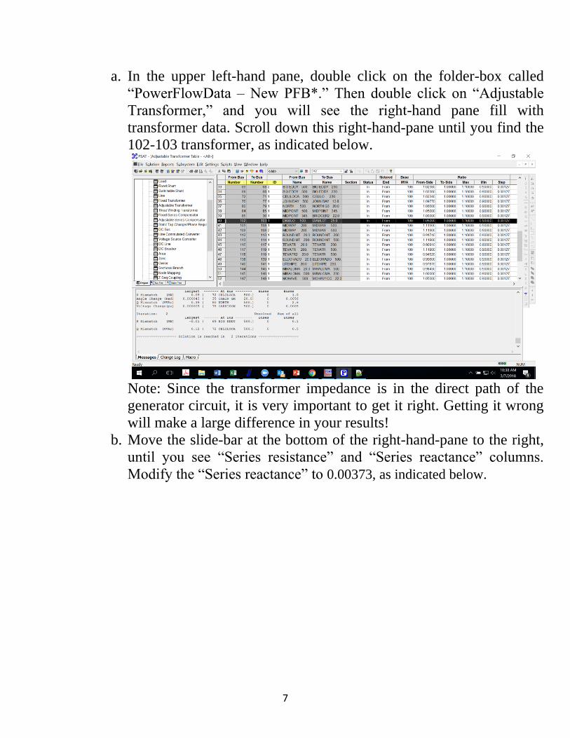
a. In the upper left-hand pane, double click on the folder-box called

“PowerFlowData – New PFB*.” Then double click on “Adjustable

Transformer,” and you will see the right-hand pane fill with

transformer data. Scroll down this right-hand-pane until you find the

102-103 transformer, as indicated below.

Note: Since the transformer impedance is in the direct path of the

generator circuit, it is very important to get it right. Getting it wrong

will make a large difference in your results!

b. Move the slide-bar at the bottom of the right-hand-pane to the right,

until you see “Series resistance” and “Series reactance” columns.

Modify the “Series reactance” to 0.00373, as indicated below.

8

8. Now modify the generator data at bus 102.

a. With the upper left-hand-pane still showing the contents of

“PowerFlowData – New PFB*,” double click on “Generator,” and

you will see the right-hand-pane fill with generator data. Scroll down

this pane until you find the bus 103 generator (Diablo 25.0), as

indicated below.

9

b. Observe under “Base MVA” that it indicates “1500.” Change this to

2680 by clicking in the appropriate cell and typing “2680,” and then

hit carriage return.

c. Observe that “MVAR Max” and MVAR Min” are 330 and -310,

respectively. Change these to 660 and -620, respectively, by clicking

in the appropriate cell and typing the correct value, then hit carriage

return. You should now see your screen as below.

9. Some final checks to make regarding the power flow data are as follows:

a. Identify the swing bus in the generator data. It will say “Swing bus”

under the “Bus type” column. You will see that it is John Day 13.8

(bus 77). Make sure that its MW output is not exceeding its rating.

This also tells you something about how much you might be able to

adjust Diablo output up and down without making any additional

manual change to generation or load. You should find that the John

Day generator has a rating of 10400MVA and an output of 5174MW.

Of course, if you use the swing bus to compensate for any changes at

Diablo, you should be aware that you are making a distinct MW

shift, and if you do not consider this MW shift to be reasonable, then

you will need to think of another MW shift that would be and then

make it. But be aware that any other desired MW shift beside using

the swing bus will require at least one additional manual change.

10

b. With the upper left-hand-pane still showing the contents of

“PowerFlowData – New PFB*,” double click on “Line,” and you

will see the right-hand-pane fill with line data. Scroll down this pane

to identify all bus 102 line connections. There should be 3 of them:

i. Bus 102 to bus 104 #1

ii. Bus 102 to bus 108 #1

iii. Bus 102 to bus 108 #2

These three are shown in between the dark row and the bottom of the

right-hand pane as indicated below. This is just to verify Figure. 2.

Note that the circuit “ID” for most circuits shown here is “1” but

some are “2” or “3”. The circuit ID can be anything, and it is

required (along with from and to buses) to uniquely identify a circuit.

You need to designate circuit ID in the switching file; it is always

important, but it is easy to get wrong if there are two or more parallel

circuits (which is the case for the two Diablo-Midway 500 kV lines).

10. Now resolve the power flow as in Step 6 above.

11. Save your power flow solution as follows:

Click on “File” in the upper left-hand menu, and select “Save

powerflow as.” A dialogue box will appear. Go to an appropriate

directory and save it as type “PFB files.” Provide it with an

appropriate name. I suggest to use “wecc179”. We refer to this file as

your power flow saved case; it contains all of the power flow data

together with the particular solution you obtained from the last solve.

11

12. Before you close out of PSAT, make sure you know how to re-open

your power flow saved case, as follows:

a. Click on “File” in the upper left-hand menu, and select “Open Power

flow.”

b. Go to the appropriate directory and select your power flow saved

case file.

c. Click on “Open.” Now you have retrieved your power flow saved

case to memory (including power flow data and a solution), and you

can make changes to it, resolve it, and resave it (perhaps to a

different name if you don’t want to overwrite your stored case).

13. Close out of PSAT by clicking on “File” and then select “exit” at the

very bottom of the menu.

B. Modifying dynamic data

In this section, we will modify the inertia constant, reactances, and time constants

of the machine as needed.

Note from the above “MF” card, we observe that the MW-sec are 4650. This

means that Hmach*MVAmach=4650MW-sec. Since this is for just one machine, with

MVA rating of 1340, we can compute Hmach=4650/1340=3.47 sec. You should

check to ensure that your data reflects this inertia.

Equivalent single machine data of 2 machine Original data in wecc179.dyr file Read as IBUS, ’GENROU’, I, T’do, T"do, T’qo, T"qo, H, D, Xd, Xq, X’d, X’q, X"d, Xl, S(1.0), S(1.2)/

103 'GENROU' 1 6.12000 0.05200 1.50000 0.14400

3.46000 0.00000 2.12900 2.07400 0.46700

1.27000 0.31100 0.25000 0.09000 0.38000 /

Correct data provided at bottom of page 3: UT

NY O

IP W

I P TE N X''D X''Q T''DT''Q

MD < NAME ><KV>D<MVA> <F> <#> <> < > < >< >< >< >

MD DIABLO CYN 211340. 90 1 N PG+ 0.2810.281.043.124

MF - CARD

--------

I P Q MVA T'D T'Q SG10 SG12 D

MF < NAME ><KV>D<MWS ><%><%>< ><RA><X'D><X'Q><XD ><XQ >< >< ><XL >< >< >< >

MF DIABLO CYN 214650.01.01.0134000210.3460.9911.6931.6366.581.5 2280.07690.410.0

Correcting the original data in the PTI format so that it agrees with the provided data:

12

1) Calculating inertia, H: Inertia Constant for 1 machine is 4650 MWs. Therefore, H = 4650/1340 MW.s/MVA= 3.47 MW.s/MVA.

2) Correcting time constants and reactances to agree with the provided data:

103 'GENROU' 1 6.58100 0.043 1.50000 0.12400

3.47000 0.00000 1.69300 1.64600 0.34600

0.991000 0.28100 0.25000 0.0769 0.41000 /

Observe that X1 is not given in the provided data and so we let it remain equal to 0.25.

3) Data to be changed to reflect a two-machine equivalent: a) Time constants: They are independent of machine rating and so stay the same b) Reactances: They will also stay the same because they are given on an MVA base equal to the machine rating. Since we have doubled the machine dating, these per-unit values will effectively be halved. b) Inertia: The two machines are assumed to be swinging together. For one unit, H=4650/1340=3.47, on the machine base. For two units, H=9300/2680=3.47, on the machine base. Either way, the inertia constant is 3.47

So the correct data for equivalent single generator to represent both units is below:

103 'GENROU' 1 6.58100 0.043 1.50000 0.12400

3.47000 0.00000 1.69300 1.64600 0.34600

0.991000 0.28100 0.25000 0.0769 0.41000 /

The above data is used to replace the old machine data in the file wecc179.dyr file. The modified dataset was saved to a new file called wecc179mod.dyr.

C. Running time-domain simulation program (TSAT)

You should go through the following steps to learn how to run the TSAT time-domain

simulation program. These instructions take you through simulation of the “normal”

conditions associated with the power flow case that resulted from following step A

above. In this case, all circuits are “in” (that is, it is NOT a weakened condition), and

the Diablo Canyon plant is generating at 765 MW. We will simulate a 3-phase –to-

ground fault at the Diablo 500 kV bus (bus 102), followed by loss of the Diablo 500

kV to Midway 500 kV circuit #1 (102-108, #1). Because all lines are in, and because

there are two Diablo units (via our equivalent) generating at only 765MW (which is

only 28.5% of full load), we should be very surprised if this case is unstable, because

it would mean that the system as designed does not satisfy the NERC reliability

criteria.

Start by bringing up TSAT.

1. Click on “File” in the top menu and select “New.” You will see the following

dialogue box. Click on “Next.”

13

2. You will then see the following dialogue box. Select the “Powerflow format” to

be “PFB, PSF.” Then click on the “Browse” button beside the “Powerflow”

window, and navigate to the folder containing your saved power flow case (in

my case, I called it wecc179.pfb). Select it by clicking “Open.”. Then click

“Next.”

14

3. You will now see a new dialogue box, where, at the top, it calls for “Dynamic

Data.” Next to the word “Default,” select PSS\E from the drop-down menu.

Also, make sure that the “Name Option” is selected to “Bus Number.” Then

click on the “Browse” button next to the “Dynamic Data Files” window.

Navigate to the directory containing your dynamic data file (in my case, I called

it wecc179mod.dyr), select it, and click “Open.” Then click “Next.”

4. You will now see a new dialogue box, where, at the top, it calls for “Monitor

Data File(s).” Make sure that the “Name Option” is selected to “Bus Number.”

Then click on the “Browse” button next to the “Monitor Data Files” window.

Navigate to the directory containing your monitor data file (in my case, I called

it Monitor.mon), select it, and click “Open.” Then click “Next.” The monitor file

posted to the website is as below. [TSAT 8.X Monitor]

{Generator}

103, ' 1'

System,0.0

{End Generator}

{Generator State}

103, ' 1', 1, 2, 0, 0

{End Generator State}

{Additional Quantities}

bus, Voltage frequency

{End Additional Quantities}

{Bus}

102

103

104

108

{End Bus}

5. You will now see a new dialogue box, where, at the top, it calls for

“Contingency File(s).” Make sure that the “Name Option” is selected to “Bus

Number.” Then click on the “Browse” button next to the “Contingency Files”

window. Navigate to the directory containing your contingency file (in my case,

I called it faultbus103.swi), and select it. Then click “Next.” The contingency

file posted to the website is as below.

15

/

/

Description Fault bus 102

Application Basecase Analysis

Simulation 10.000000 Seconds

Step Size 0.5 Cycles

Plot 2 Steps

Report 2 Steps

Integration RK4

After 1 Seconds

Three Phase Fault At Bus ;102

After 4 Cycles

Clear Three Phase Fault

Remove Line ;102 ;108 ;1

Nomore

/

END

6. You will now see a new dialogue box, where, at the top, it calls for “Criteria

Data.” We will not use that, so click on “Next.”

7. You will now see a new dialogue box, where, at the top, it calls for “Dynamic

Representation Data File.” We will not use that, so click on “Next.”

8. You will now see a new dialogue box that calls for several additional optional

data files, including “Transfer File,” “Parameter File,” etc. We will not use

these, so click on “Next.”

9. You will now see a new dialogue box, where, at the top, it calls for “Sequence

network data file.” We will not use that, so click on “Next.”

10. You will now see a new dialogue box, where, at the top, it calls for “PMU

data file.” We will not use that, so click on “Next.”

11. You will now see a new dialogue box, where, at the top, it calls for “Title,”

and it has “Base Scenario” already entered. Click on “Next.”

12. You will now see a new dialogue box, which provides a list of all possible

data to be used by TSAT (Description, parameters, powerflow data, dynamic

data, monitor data, criteria data, contingency data, dynamic representation data,

transaction data, sequence network data, and PMU data). Click on “Save” at the

bottom of the dialogue box. It will then ask you for a file name; I suggest using

“base”.

13. You will now see the following screen.

16

To run TSAT, click on the “Run” selection from the menu at the top. Select “No

disturbance test.” A dialogue box will pop up asking you for simulation length,

step size, and integration method, with defaults of 10.00, 0.0040, and RK4,

respectively. Just leave them as defaults, and click “OK.” You will then see the

progression of the simulation in the lower right-hand-screen. When the 10

seconds of simulation are complete, you should observe all flat lines for both the

generator rotor angles and the bus voltages, as indicated below (if you don’t,

then something is wrong with your data).

17

14. Assuming your no-disturbance case ran smoothly, you can now run the

simulation of the faulted condition. To do this, click on the “Run” selection from

the menu at the top. Select “Base case analysis.” You will again observe the

progression of the simulation in the lower right-hand-pane, but these plots

should not be straight lines. In particular, the bus voltage plot at the bottom

should show the voltage at t=1 second taking a step-change drop for the first 4

cycles after the 1 second point, as indicated below.

15. Although the above views allow you to see some plots of generator angle

and bus voltages, there is a plotting routine for which you will have greater

capabilities to inspect various quantities and tailor-make them according to your

needs. To access this plotting function, click on “View” at the top and select

“Results” from the menu. A new screen will appear, as shown below.

18

16. You may like to modify the “external” part of the new screen so that it is

full screen by clicking (as usual) in the “box” button at the top-right-hand-corner

of the screen. It will then appear as below.

19

17. You might also like to make the “internal” part of the screen so that it is

full screen within the external part. You can do this by clicking on the “box”

button just to the left of the red “X”. It will then appear as below.

18. The current view consists of the terminal voltages of all generators in the

system. All of these generators are listed in the upper middle screen called

“Curve legend.” If we wanted to view only a subset of them, we could click on

the desired bus in the “Curve legend” screen. For example, let’s look at the bus

103 terminal voltage (Diablo) and the bus 77 terminal voltage (John Day), by

selecting them using CNTRL-LEFT_CLICK, which will result in the following:

20

Then right-click on one of the selected quantities (either one) and a menu will

pop up. Select “Selected quantities,” and you will then see the following:

19. Now we may like to view additional types of plots. We can observe what

is available to us (by virtue of what is contained in our “Monitor.mon” file) by

21

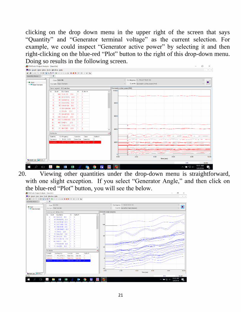
clicking on the drop down menu in the upper right of the screen that says

“Quantity” and “Generator terminal voltage” as the current selection. For

example, we could inspect “Generator active power” by selecting it and then

right-clicking on the blue-red “Plot” button to the right of this drop-down menu.

Doing so results in the following screen.

20. Viewing other quantities under the drop-down menu is straightforward,

with one slight exception. If you select “Generator Angle,” and then click on

the blue-red “Plot” button, you will see the below.

22

The fact that all angles are continuously increasing with time is because we are

viewing absolute rotor angle. If we want to view relative rotor angle, then we

need to click on “Graph” in the menu on the upper left-hand-side of the screen.

Then select “Options,” and then select “Plot relative angle.” It will use the

power flow swing bus as the reference, in this case, that bus is bus 77 (John

Day). Doing so produces the following screen.

21. Let’s now inspect generator speed for several generators, including Diablo

Canyon, plot them, and then make a PDF file that we could include in a report.

To do this, we start by selecting and plotting the generator speed quantities for

all generators. This appears as below.

23

22. Then, lets include only the top 6 generators in the list of the middle upper

pane; observe that Diablo is at the top of this list. Others on this list include

Bridger2, CanadG1, Castai4G, CMAIN GM, and CORONADO. We select them

using CNTRL-Left-Click, and then we plot them by Right-Clicking on any one

of them in the middle upper pane, and selecting “Selected Quantities.” The

below screen appears:

24

23. We can then print this by clicking on the “File” button in the top left-hand

menu, and selecting “Print.” A dialogue box will appear as below. To the right

of “Name,” select “Adobe PDF” and then click “OK.”

24. You will then be asked for location and file name of where to store the

PDF file. Navigate to your desired directory (or if you are sending to your U

drive, type in \\my.files.iastate.edu\engr\sites\home\USERNAME\FOLDERNAME\FILENAME.pdf (where USERNAME is your netID, FOLDERNAME is the folder where you are

storing your files, and FILENAME.pdf is the name of the printed pdf file) and

give an appropriate file name. I chose “Speed.pdf.” After a few seconds, the pdf

file popped up on the screen. I used the “Edit” function of Adobe, selected

“Take a snapshot,” and cut out the below figure.

25

In the above plot (which was done on my machine in my office, and not

via the VDI setup), it is satisfying to note that, although all six machines incur

speed deviation, it is clear that the one with the most speed deviation (and

therefore the one with the most acceleration and deceleration), is Diablo, which

is the one closest to the fault.

When I did all of the above on the VDI setup, everything worked perfectly,

until this point, when my pdf file looked as below, where it is clear that fonts are

somehow misconfigured. I am unsure why the fonts are misconfigured.

26

However, I repeated the print process but this time, instead of selecting

“Adobe pdf” in step 23, I selected “Microsoft Print to PDF.” I had to give it a

filename, to which it printed. Then when I opened the pdf file, the fonts were

fine.

25. Now you will need to get to work by doing the following things:

a. Modify the power flow to remove one of the Diablo-Midway lines

(suggest to remove Diablo-Midway #2 so that you can continue using the

existing switching file).

b. Modify the switching file as necessary (if you followed my suggestion in

(a), you will not need to do anything here).

c. Rerun the case, determine whether it is stable or unstable.

d. Modify the power flow to increase or decrease Diablo output as necessary

(with some appropriate compensating change, as you think best).

e. Rerun the case, determine whether it is stable or unstable. Go to (d) and

repeat until you have determined the limit.

f. Make appropriate plots to confirm the limit.

26. Repeat (25) for the case of one Diablo-Midway line out, with the

contingency being loss of the Diablo-Gates line.

27. Repeat (25) for the case of the Diablo-Gates line out, with the contingency

being loss of a Diablo-Midway line.

27

28. Develop a report that summarizes your finding. Your report should be

done professionally, with the thought being that it will first go to your supervisor

and then outside the organization (e.g., to other companies including the ISO

and the RTO).

Last comment: I ran a case with Diablo-Gates out and then simulated loss of

Diablo-Midway #1, with Diabl0 generating at 2440 MW. The result was below.

28

APPENDIX: Q-cards for provided data on Diablo Canyon machine.

*********************************************************************************

THE BELOW CONTAINS Q-CARDS FOR DATA ENTRY FOR THE WSCC TRANSIENT STABILITY PROGRAM (MACHINE

DATA ONLY)

********************************************************************************

NOTE: THESE Q-CARDS ARE HELPFUL WHEN TRYING TO READ OR TYPE TRANSIENT STABILITY

DATA FROM OR ONTO THE SCREEN. YOU CAN INSERT THEM DIRECTLY INTO THE DATA

FILE YOU ARE WORKING ON, JUST ABOVE THE DATA CARD OF INTEREST, AND THEN

VERY EASILY READ OR TYPE YOUR DATA. REFER TO THE WSCC TRANSIENT STABILITY

MANUAL FOR MORE EXPLICIT INFORMATION REGARDING DATA FORMATS.

MD- CARD

--------

UT

NY O

IP W

I P TE N X''D X''Q T''DT''Q

MD < NAME ><KV>D<MVA> <F> <#> <> < > < >< >< >< >

MF - CARD

--------

I P Q MVA T'D T'Q SG10 SG12 D

MF < NAME ><KV>D<MWS ><%><%>< ><RA><X'D><X'Q><XD ><XQ >< >< ><XL >< >< >< >

EXCITER - FIRST CARD (NEW FORMAT)

--------------------

T

Y

P

E I VI OR VA KA TA VR OR VA KE

F < NAME ><KV>D<RC ><XC ><TR ><MAX><MIN><TB ><TC ><KV ><TRH><MAX><MIN><KL ><TE>

EXCITER - SECOND CARD (NEW FORMAT)

--------------------

E/V

EFD EFDM

I SE1 SE2 EFDN VEM KF TF KD KB KL KH VLR

FZ < NAME ><KV>D<KI ><KP ><0P ><VBM><KG ><VGM><KC ><XL ><VLV><KLV><KN ><KR >< >

EXCITER - OLD CARD

------------------

T

Y

P KS EFD

E I KA TRH TA1 SE SE EFD VB KF

E < NAME ><KV>D<TR><KV ><TA>< ><VR><KE><TE><KI><KP><MIN><MAX<KA><TF><XL ><TFI>

PSS

----------------

T

Y t6 t5 t2 t1 t4 t3

P VS V

29

E IKQV TQV KQSTQS TQ1 T'Q1TQ2 T'Q2TQ3 T'Q3 MAX CUTVS

S < NAME ><KV>D< >< >< >< ><TQ>< >< >< >< >< >< >< >< ><><REMOTE BUS>

GOVERNOR AND TURBINE CARD -TYPES H & C

--------------------------------------

H I PMAX R TG TP TD .5TW VELC VELO DO <- TYPE H HYDRO

GC < NAME ><KV>D<PMAX>< R ><T1 ><-- ><T3 ><T4 ><T5 >< F ><DH > <- TYPE C CROSS-COMPOUND

GOVERNOR AND TURBINE CARD -TYPES S & W

--------------------------------------

VEL VEL

S I PMAX PMIN R T1 T2 T3 OPEN CLOSE <- TYPE S STEAM GOVERNOR

GW < NAME ><KV>D<PMAX><PMIN>< R ><T1 ><T2 ><T3 >< >< > <- TYPE W HYDRO-GOVERNOR

TURBINE CARD - TYPES S & W

--------------------------

T

Y

P

E I

T < NAME ><KV>D<T4 ><K1 ><K2 ><T5 ><K3 ><K4 ><T6 ><K5 ><K6 ><T7 ><K7 ><K8 >