Reports Meteorology and Climatology

No 101, Jan 2003

Jouni Räisänen, Ulf Hansson, Anders Ullerstig,Ralf Döscher, L. Phil Graham, Colin Jones,Markus Meier, Patrick Samuelsson and Ulrika WillénRossby Centre

GCM driven simulations of recent andfuture climate with the Rossby Centrecoupled atmosphere – Baltic Searegional climate model RCAO

Cover illustration: Changes in mean annual precipitation (in per cent of the control runmean) in the HadAM3H-driven (left) and the ECHAM4/OPYC3-driven (right) regionalclimate change simulations.

RMK No. 101, January 2003

GCM driven simulations of recent and future climate with theRossby Centre coupled atmosphere – Baltic Sea regionalclimate model RCAO

Jouni Räisänen, Ulf Hansson, Anders Ullerstig, Ralf Döscher, L. Phil Graham, ColinJones, Markus Meier, Patrick Samuelsson and Ulrika Willén

Rossby Centre, SMHI

Report Summary / RapportsammanfattningIssuing Agency/Utgivare

Swedish Meteorological and Hydrological Institute

Report number/Publikation

RMK No. 101S-601 76 NORRKÖPINGSweden

Report date/Utgivningsdatum

January 2003

Author (s)/Författare

Jouni Räisänen, Ulf Hansson, Anders Ullerstig, Ralf Döscher, L. Phil Graham, Colin Jones, MarkusMeier, Patrick Samuelsson and Ulrika Willén

Title (and Subtitle/Titel

GCM driven simulations of recent and future climate with the Rossby Centre coupled atmosphere –Baltic Sea regional climate model RCAO

Abstract/Sammandrag

A series of six general circulation model (GCM) driven regional climate simulations made at the RossbyCentre, SMHI, during the year 2002 are documented. For both the two driving GCMs HadAM3H andECHAM4/OPYC3, a 30-year (1961-1990) control run and two 30-year (2071-2100) scenario runs have beenmade. The scenario runs are based on the IPCC SRES A2 and B2 forcing scenarios. These simulations weremade at 49 km atmospheric resolution and they are part of the European PRUDENCE project.

Many aspects of the simulated control climates compare favourably with observations, but some problemsare also evident. For example, the simulated cloudiness and precipitation appear generally too abundant innorthern Europe (although biases in precipitation measurements complicate the interpretation), whereas tooclear and dry conditions prevail in southern Europe. There is a lot of similarity between the HadAM3H-driven (RCAO-H) and ECHAM4/OPYC3-driven (RCAO-E) control simulations, although the problemsassociated with the hydrological cycle and cloudiness are somewhat larger in the latter.

The simulated climate changes (2071-2100 minus 1961-1990) depend on both the forcing scenario (thechanges are generally larger for A2 than B2) and the driving global model (the largest changes tend to occurin RCAO-E). In all the scenario simulations, the warming in northern Europe is largest in winter or autumn.In central and southern Europe, the warming peaks in summer and reaches in the RCAO-E A2 simulationlocally 10°C. The four simulations agree on a general increase in precipitation in northern Europe especiallyin winter and on a general decrease in precipitation in southern and central Europe in summer, but themagnitude and the geographical patterns of the change differ a lot between RCAO-H and RCAO-E. Thisreflects very different changes in the atmospheric circulation during the winter half-year, which also have alarge impact on the simulated changes in windiness. A very large increase in the lowest minimumtemperatures occurs in a large part of Europe, most probably due to reduced snow cover. Extreme dailyprecipitation increases even in most of those areas where the mean annual precipitation decreases. Key words/sök-, nyckelord

Climate change, climate scenario, regional climate modelling, Europe, PRUDENCESupplementary notes/Tillägg

This work is a part of the SWECLIM programmeand of the EU PRUDENCE project.

Number of pages/Antal sidor

61Language/Språk

English

ISSN and title/ISSN och title

0347-2116 SMHI Reports Meteorology ClimatologyReport available from/Rapporten kan köpas från:

SMHIS-601 76 NORRKÖPINGSweden

Contents

1 Introduction ............................................................................................................ 12 The experimental design ........................................................................................ 1

2.1 The coupled regional climate model RCAO .................................................... 12.2 The driving GCM simulations.......................................................................... 32.3 Representation of forcing in RCAO ................................................................. 42.4 Spin-up ............................................................................................................. 42.5 The ice thickness problem ................................................................................ 52.6 Output parameters of the atmospheric model................................................... 6

3 The control simulations.......................................................................................... 63.1 Sea level pressure ............................................................................................. 73.2 Total cloudiness................................................................................................ 73.3 Surface air temperature..................................................................................... 9

3.3.1 Time mean temperature ............................................................................ 93.3.2 Interannual variability of monthly mean temperatures ............................. 93.3.3 Diurnal temperature range ...................................................................... 113.3.4 Temperature extremes ............................................................................ 12

3.4 Precipitation.................................................................................................... 133.4.1 Time mean precipitation......................................................................... 133.4.1 Interannual variability of monthly precipitation ..................................... 143.4.2 Number of precipitation days ................................................................. 153.4.3 Extreme daily precipitation..................................................................... 16

3.5 Wind speed ..................................................................................................... 173.5.1 Time mean wind speed ........................................................................... 173.5.2 Extremes of wind speed.......................................................................... 18

3.6 Snow conditions ............................................................................................. 183.7 Other aspects of the surface hydrology........................................................... 203.8 Ice conditions.................................................................................................. 21

3.8.1 Lake ice................................................................................................... 213.8.2 Baltic Sea ice cover ................................................................................ 22

4 Simulated climate changes for the period 2071-2100 ........................................ 234.1 Sea level pressure ........................................................................................... 23

4.1.1 Time mean sea level pressure ................................................................. 234.1.2 Band-pass filtered variability.................................................................. 25

4.2 Total cloudiness.............................................................................................. 264.3 Surface air temperature................................................................................... 27

4.3.1 Time mean temperature .......................................................................... 274.3.2 Interannual variability of monthly mean temperatures ........................... 294.3.3 Diurnal temperature range ...................................................................... 304.3.4 Temperature extremes ............................................................................ 31

4.4 Precipitation.................................................................................................... 324.4.1 Time mean precipitation......................................................................... 324.4.2 Interannual variability of monthly precipitation ..................................... 344.4.3 Number of precipitation days ................................................................. 354.4.4 Extreme daily precipitation..................................................................... 37

4.5 Wind speed ..................................................................................................... 384.5.1 Time mean wind speed ........................................................................... 384.5.2 Extremes of wind speed.......................................................................... 39

4.6 Snow conditions ............................................................................................. 394.7 Other aspects of the surface hydrology........................................................... 41

4.7.1 Evaporation............................................................................................. 414.7.2 Runoff generation ................................................................................... 424.7.3 Soil moisture........................................................................................... 43

4.8 Ice conditions.................................................................................................. 444.8.1 Lake ice................................................................................................... 444.8.2 Baltic Sea ice cover ................................................................................ 45

5 Statistical analysis of simulated climate changes............................................... 465.1 Simulated changes versus internal variability ................................................ 465.2 Comparison between RCAO-H and RCAO-E ............................................... 515.3 Climate change in Sweden ............................................................................. 52

6 Conclusions ........................................................................................................... 55Acknowledgments......................................................................................................... 57Appendix. Modification of the RCAO-H monthly mean files to reduce the icethickness problem......................................................................................................... 57References...................................................................................................................... 58

1

1 IntroductionThe Rossby Centre, part of SMHI and the Swedish Regional Climate ModellingProgramme SWECLIM, has recently conducted a set of new regional climate changesimulations. Six 30-year regional model runs have been made, using boundary data fromthe two global general circulation models (GCMs) HadAM3H and ECHAM4/OPYC3.Two of these runs represent the recent (1961-1990) climate and the remaining four theclimate in the late 21st century (2071-2100) under two different assumptions of futureatmospheric composition. These simulations contribute to the European PRUDENCEproject.

This report gives an overview of the results of the mentioned simulations. Both thequality of the simulated recent climate (1961-1990) and the climate changes projectedfor 2071-2100 are discussed, with some more emphasis on the latter. The focus islargely on the atmospheric near-surface climate, including both the time mean state andsome measures of variability and extremes. However, it is impossible to cover allrelevant topics in one report. For example, user-oriented parameters like growing seasonlength, wind energy potential, heating or cooling degree days etc. are excluded here.Another important question that we do not address explicitly is comparison between theregional climate model and the driving GCM simulations. However, the differencesbetween our HadAM3H- and ECHAM4-driven experiments underline the point thatmany aspects of regional climate simulations are strongly governed by the drivingGCM. This conclusion is well in line with earlier research (e.g., Noguer et al. 1998;Rummukainen et al. 2001; Räisänen et al. 2001).

The outline of this report is as follows. We first describe the regional climate model, theGCMs that provided boundary data for it, the emission scenarios used in the climatechange simulations, and other issues related to the design of the experiments (Section2). In Section 3, the control simulations (1961-1990) are discussed and compared withobservational estimates of climate in the same period. After this, the projected climatechanges for the period 2071-2100 are studied. First, in Section 4, a descriptive overviewof the simulated changes is given. Then, in Section 5, some statistical aspects areaddressed, including the significance of the changes with respect to unforced climatevariability and the relative similarity, or lack thereof, between the results of theHadAM3H- and ECHAM4-driven simulations. Finally, the conclusions are given inSection 6.

2 The experimental design

2.1 The coupled regional climate model RCAOThe coupled regional climate model RCAO consists of the atmospheric model RCA2(Jones 2001; Bringfelt et al. 2001), the three-dimensional Baltic Sea ocean model RCO(Meier et al. 1999; Meier 2001; Meier et al. 2002) and the lake model PROBE(Ljungemyr et al. 1996) applied in an area approximately covering the Baltic Seadrainage basin. In the experiments described here the atmospheric model was run in a

2

rotated latitude-longitude grid with a resolution of 0.44° (approximately 49 km) in bothhorizontal directions and with 24 levels in the vertical. The integration domain coveredan area of 106 ×102 grid boxes, of which the outermost eight at each side were used asboundary relaxation zones. The ocean model RCO was run with 6 nm (approximately11 km) horizontal resolution and with 41 levels in the vertical, in an area covering theBaltic Sea and the Kattegat.

The atmospheric model domain is shown in Fig. 1, which also indicates four subregionsused for portraying the results. The ones that are most frequently used are Sweden(which is of special interest from a local Swedish perspective but also often gives agood idea of the results in northern Europe in general) and land south of 49°N (whichprovides a general impression of the model behaviour in the southern half of thedomain). Only grid boxes with at least 50% of land are included in these two areas.Where space admits and this gives significant additional information, some area meansare also shown for the whole Baltic Sea runoff area (including Sweden but excluding theBaltic Sea) and the Baltic Sea itself. As also indicated in Fig. 1, most figures in thisreport exclude the boundary relaxation zones and the two outermost rows and columnsin the ordinary model area, which are still very markedly affected by boundary problemssuch as sharp gradients in cloudiness and precipitation.

Figure 1. The RCAO model domain. The outer dashed lines indicate the boundary relaxationzones and the inner dashed lines the area shown in most figures of this report andused for the statistics in Section 5. Also shown are four subareas for which some ofthe results are shown separately: Sweden, the Baltic Sea runoff area (whichincludes Sweden), the Baltic Sea and land south of 49˚N.

Since the focus in this report is on atmospheric and land surface results, the mainfeatures of RCA2 are discussed in some more detail below. The model is structuredwithin the HIRLAM reference system and uses the HIRLAM model semi-Lagrangiandynamical core described in McDonald and Haugen (1992, 1993) with 6th order implicithorizontal diffusion (McDonald 1994). However, most of the original HIRLAMphysical parameterisations have been exchanged for newer schemes. The fast but highlysimplified radiation scheme described in Savijärvi (1990) and Sass et al. (1994) is still

3

used, but with some modifications added by Räisänen et al. (2000b) to allow, inparticular, changes in the CO2 concentration between different model runs. Subgridscale vertical mixing is treated with the scheme of Cuxart et al. (2000), which includesturbulent kinetic energy as a prognostic variable. The Kain-Fritsch convection scheme(Fritsch and Chappell 1980; Kain and Fritsch 1990) parameterises both deep andshallow convective mixing. The parameterisation of resolved condensation processesfollows that described in Rasch and Kristjánsson (1998). Cloud water is a prognosticvariable, whereas resolved cloud fraction is diagnosed from relative humidity followingSlingo (1987). There is a tight coupling between convection and resolved condensationwith detrained convective cloud water and moisture acting as a source term for resolvedcondensation within the same time step. Finally, the land surface-soil scheme has twoprognostic layers for temperature and soil moisture, plus an additional bottomtemperature layer whose temperature is derived from the driving GCM simulation. Aweighted vegetation fraction is used to parameterise the effect of vegetation on theprognostic variables. A full description of the surface-soil scheme can be found inBringfelt et al. (2001).

2.2 The driving GCM simulationsData from two global climate models, HadAM3H and ECHAM4/OPYC3, were used todrive RCAO. ECHAM4/OPYC3 (Roeckner et al. 1999) is a coupled atmosphere-oceanGCM, whose atmospheric component ECHAM4 was run at T42 spectral resolution(formally equivalent to a grid spacing of 2.8° lon × 2.8° lat). HadAM3H is a high-resolution (1.875° lon × 1.25° lat) version of the atmospheric component of the HadleyCentre coupled atmosphere ocean GCM HadCM3 (Gordon et al. 2000). BecauseHadAM3H excludes the ocean, the simulations with this model used sea surfacetemperature (SST) and sea ice distributions derived from observations and earlier, lowerresolution HadCM3 climate change experiments (see below).

The two coupled atmosphere-ocean models HadCM3 and ECHAM4/OPYC3 were firstrun from 1860 to 1990, using observed or estimated changes in atmosphericcomposition. From 1990 on, the simulations were divided to two using two differentscenarios of future anthropogenic greenhouse gas and aerosol emissions: IPCC SRESA2 and B2 (Nakićenović et al. 2000). The A2 scenario assumes relatively large (incomparison with the other SRES scenarios) and continuously increasing emissions ofthe major anthropogenic greenhouse gases, CO2, CH4 and N2O. The B2 scenario alsofeatures an increase in the CO2 and CH4 emissions, but this is slower, in the lowermidrange of the SRES scenarios. However, sulphur emissions are also larger in A2 thanin B2, which partly compensates the climatic effects of the larger greenhouse gasemissions.

For driving RCAO, two 30-year time slices (1960/1961-1990 and 2070-2100) of theHadAM3H and ECHAM4/OPYC3 simulations were used. HadAM3H itself was run forthese periods only, using presecribed SST and sea ice distributions. For the control run(1960-1990), observed sea surface conditions were used. For the period 2070-2100, theSST and ice distributions were modified using the HadCM3-simulated changes in SSTand ice. For SST the modification was relatively simple. The HadCM3-simulatedchange in SST was represented by its 30-year seasonally varying mean value (2071-2100 minus 1961-1990) plus the best-fit linear trend within the 30-year period (toaccount for the increase in greenhouse gases from 2070 to 2100). This change was then

4

added to the observed SST time series for 1960-1990. For sea ice, the principle was thesame but a slightly more complicated adjustment procedure was needed to account forthe differences in ice edge between HadCM3 in 1961-1990 and the observations(http://dmiweb.dmi.dk/pub/prudence/hadam3h_ hadrm3h_ info.html).

The motivation to not employ HadCM3 data directly to drive regional climate modelsderives from the relatively poor control climate in HadCM3, which does not use fluxadjustments. There are substantial biases in SST in some ocean areas including thenorthern North Atlantic (Gordon et al. 2000), as well as in aspects of the simulatedatmospheric climate. For example, the annual mean surface air temperatures in Swedenare about 3°C too low. The use of observed SSTs and the higher resolution inHadAM3H allowed a more realistic control climate, even though it is not possible toverify that the simulation of climate changes was also improved.

2.3 Representation of forcing in RCAOThe IPCC SRES scenarios include changes in the concentrations of several atmosphericgreenhouse gases and aerosol types. Because of the simplicity of the RCA2 radiationcode, the net effect of these changes was approximated by an “equivalent” increase inthe CO2 concentration. The control run value of 353 ppmv was raised in the B2simulations to 822 ppmv and in the A2 simulations to 1143 ppmv, which values wereheld constant over the whole 30-year period. These values were selected so that theresulting increase in global mean radiative forcing, approximated followingRamaswamy et al. (2001, p. 358) as

])CO(ln[ Wm35.5 22���

�F (1)

would equal the projected 2071-2100 minus 1961-1990 changes in total anthropogenicradiative forcing for the B2 and the A2 scenarios, respectively. The estimates for thelatter (4.5 W m-2 for B2 and 6.2 W m-2 for A2) were obtained from Houghton et al.(2001, pp. 66 and 823). This method of treating the forcing is crude, but it is justified bythe fact that the sensitivity of regional climate models to the local radiative forcing issmall (Räisänen et al. 2000, 2001). The model feels the “global warming” mainlythrough the change in boundary conditions, that is, through the inflow of warmer andmoister air from the driving global model and through the higher prescribed SSTs and(in the case of RCA2) deep soil temperatures. Note that the actual projected increases inthe CO2 concentration are smaller, with values reaching slightly over 600 and nearly 850ppmv by 2100 in the B2 and A2 scenarios, respectively (Houghton et al. 2001, p. 65).

2.4 Spin-upThe atmospheric results shown in this report were calculated using the full simulated30-year periods 1961-1990 and 2071-2100. These 30-year periods were preceded by a 4-month spin-up period, which in all three HadAM3H-based runs (hereafter RCAO-H)and the ECHAM4/OPYC3-based (hereafter RCAO-E) A2 and B2 scenario runs usedboundary data for the autumn 1960 or 2070. However, because ECHAM4/OPYC3boundary data were not available at a sufficient time resolution in 1960, the RCAO-Econtrol run spin-up was made using boundary data for September-December 1961. Thisprocedure creates an abrupt change in boundary conditions between the end and therebeginning of the year 1961, but at least in the atmosphere, the resulting shock wasfound to die out within the first two simulated days of the new year.

5

The Baltic Sea model RCO was initialised using observational data for September 1960,both for the control and the scenario runs. The use of observations to initialise thescenario runs is problematic, since the observed water temperatures in 1960 are notrepresentative of the simulated warmer climate in the 2070’s. We therefore exclude thefirst winter (2070-2071) when discussing the simulated changes in Baltic Sea iceconditions. Although this problem may also have an effect on the atmosphericconditions around the Baltic Sea in the year 2071, this effect appears to be small incomparison with the interannual variability.

2.5 The ice thickness problemIn the RCAO-H simulations, an instability in the PROBE lake model occasionallygenerated abrupt, unphysically large increases in ice thickness. As a result, the icethickness in some lakes exceeded 10 meters in some winters, and the thick ice coveroccasionally survived over the following summer (see Fig. 2a for an example). Theproblem only occurred in deep lakes that include, in the RCAO implementation ofPROBE, Lake Ladoga, Lake Onega and a number of Swedish lakes.

An excessively thick ice cover affects the overlaying atmosphere, particularly thesurface air temperature in summer. To approximately correct for this problem, themonthly mean files were rewritten applying a simple adjustment scheme to those gridboxes where the ice thickness had exceeded 1.5 m during the previous nine months(Appendix). Comparison between the original and adjusted files indicates that theproblem had a serious impact only over large lakes (such as Lake Ladoga) that cover asubstantial fraction of an atmospheric grid box (see Fig. 2b). In most of those about 60grid boxes (less than 1% of the model area) where adjustments were made, the two setsof files are almost identical. No such adjustments have been made to the daily and thesix-hourly files, however.

Figure 2. (a) Ice thickness in Lake Siljan (60.9°N, 14.8°E) in the RCAO-H control run. (b)Difference (°C) in June-July-August mean 2 m temperature between the originaland adjusted files (original minus adjusted) in the RCAO-H control run. Thedifferences in the other seasons are smaller.

This problem was detected when analysing the RCAO-H control run, but forconsistency the same version of PROBE was used even in the two RCAO-H scenario

6

runs. For all the RCAO-E simulations, the problem was eliminated by a simple fix to thePROBE model code.

2.6 Output parameters of the atmospheric modelA list of the saved RCA2 output parameters and their time resolution is given Table 1.

Table 1. The RCA2 output and its time resolution. 6H indicates instantaneous six-hourlyvalues, and 24H and M daily and monthly means estimated from these. The valuesmarked as 6H* are means or extremes over the previous six hours, and 24H* andM* daily and monthly means or extremes calculated from these. M** is the monthlymean of daily extremes. MC indicates monthly means stored separately for differenttimes of the day (00, 06, 12 and 18 UTC). Surf = surface; LW = long-wave; SW =short-wave.

Pressure level data (300, 500, 700, 850 and 925 hPa) Fluxes of water (continued)Temperature M + 500 and 850 hPa 6H Evaporation M*, 24H*Wind components M + 500 and 850 hPa 6H Interception evaporation M*, 24H*Relative humidity M + 500 and 850 hPa 6H Runoff M*, 24H*Vertical velocity (�) M + 500 and 850 hPa 6HGeopotential height M + 500 and 850 hPa 6H Other surface data

Temperature, 2 m M, MC, 24H, 6HOther free atmospheric data Max temperature, 2 m M**, 24H*Integrated water vapor M, 6H Min temperature, 2 m M**, 24H*Integrated cloud water M, MC Soil temperature (top) M, 6HLow cloud cover M, MC Max soil temperature (top) M**, 24H*Mid-level cloud cover M, MC Min soil temperature (top) M**, 24H*High cloud cover M, MC Soil temperature (deep) M, 24H

Soil temperature (bottom) MFluxes of energy, water and momentum Soil moisture (top) M, 24HLatent heat flux (surf) M*, 6H* Soil moisture (deep) M, 24HPotential latent heat flux M*, 6H* Wind components, 10 m M, 6HSensible heat flux (surf) M*, 6H* Max wind speed, 10 m 6H*Momentum flux (surf) M*, 6H* Mean wind peed, 10 m MNet SW radiation (surf) M*, 6H* Relative humidity, 2 m M, 6HNet LW radiation (surf) M*, 6H* Sea level pressure M, 6HDownward SW rad. (surf) M*, 6H* Surface pressure M, 6HDownward LW rad. (surf) M*, 6H* Total cloud cover M, 6HNet SW radiation (top) M*, MC* Sunshine hours M*, 24H*Net LW radiation (top) M*, MC* Snow water equivalent M, 24HDownward SW rad. (top) M* Snow fraction M, 24HPrecipitation M*, 24H* Ice cover M, 24HLarge-scale precipitation M*, 6H* Ice thickness M, 24HConvective precipitation M*, 6H* Water temperature M, 24HSnowfall M*, 6H*

3 The control simulationsIn this section, the control period (1961-1990) climates in the HadAM3H-driven(RCAO-H) and ECHAM4/OPYC3-driven (RCAO-E) regional experiments arediscussed and compared with observational estimates of the climate in this period. Thefocus is on surface and near-surface climate and mainly on time-mean conditions. For afew variables (surface air temperature, precipitation and wind speed), aspects of

7

variability and extremes are also discussed. For an overview of the order of discussion,the reader is referred to the table of contents. Because of the importance of thesevariables for interpreting some of the temperature- and precipitation-related results, thediscussion begins from sea level pressure (Section 3.1) and total cloudiness (Section3.2).

3.1 Sea level pressureThe gross features of the observed time mean sea level pressure are well reproduced inthe RCAO control simulations, that is, the biases are generally small compared with theoverall geographical variation (Fig. 3). The biases that do exist tend to be of somewhatlarger magnitude in RCAO-E than in RCAO-H. The pressure in the RCAO-E simulationis, in most of the year, too high in the southwestern and northeastern parts of thedomain, with a smaller (positive or negative) bias in-between. This indicates toocyclonic time-mean conditions (and possibly too frequent cyclone activity) in the middleof the domain. The biases in RCAO-H are more seasonally variable. For example, thepattern in winter indicates too strong westerly flow from the Atlantic Ocean to southernScandinavia and the western parts of central Europe, whereas the reverse is true inspring and autumn.

Figure 3. Top: seasonal (DJF = December–February, MAM = March–May, JJA = June–August, SON = September–November) and annual (ANN) means of sea levelpressure in 1961-1990 (contours every 2 hPa) according to the NCEP reanalysis(Kalnay et al. 1996; Kistler et al. 2001). Middle and bottom: the differences RCAO-H – NCEP and RCAO-E – NCEP (contours and shading at ±1, ±3, ±5 and ±7 hPa).The maps show the whole RCAO domain, including the boundary relaxation zones.

3.2 Total cloudinessThe analysis of surface observations by CRU, the University of East Anglia ClimateResearch Unit (New et al. 1999, 2000) reveals a contrast in annual mean cloudinessbetween northern and southern Europe, with more clouds in the north than in the south(Fig. 4). The north-south contrast in the RCAO simulations is qualitatively similar but

8

stronger. The northern half of the model domain is, on the average, too cloudy incomparison with the CRU climatology, and the southern half too clear. Qualitatively thesame pattern of biases was found in the reanalysis-driven RCA2 simulations analysed byBringfelt et al. (2001) although, in these, the positive bias in northern Europe wassmaller.

The bottom two panels of Fig. 4 show the 30-year mean seasonal cycles of cloudinessaveraged over Sweden and the land area south of 49ºN. The positive bias in cloudinessin Sweden and elsewhere in northern Europe persists througout the year, being in thesummer half-year larger in RCAO-E (in which the pressure pattern indicates morecyclonic flow conditions) than in RCAO-H. The annual mean cloudiness in Sweden is66% in the CRU data set, 77% in RCAO-H and 80% in RCAO-E. In the land area southof 49ºN, both simulations appear to underestimate the average cloudiness in almost allmonths (although there are large variations within this area), with a larger underestimatein RCAO-E than in RCAO-H

Figure 4. Top: annual mean total cloudiness (%) from the CRU climatology (land only) and inthe RCAO-H and RCAO-E control simulations. Bottom: the seasonal cycles ofcloudiness from CRU (black), RCAO-H (red) and RCAO-E (blue) in Sweden and inthe land area south of 49°N. The boundary relaxation zones and the two outermostrows and columns in the ordinary model area are excluded from the figure. In (a)-(c), the shading interval is 5%, but contours are drawn at every 10% only and thelabels are excluded for legibility.

The CRU cloud climatology itself is not an exact truth. When the sun is under thehorizon, surface observations tend to underestimate the true cloud cover, because thinclouds remain easily unnoticed (e.g., Hahn et al. 1995). Conversely, high cumulus- orcumulonimbus clouds (which are most common in summer, and more common in the

9

southern than the northern parts of the RCAO domain) generally seem to cover a largerpart of the sky than is their actual projection against the Earth surface (the quantitysimulated by models). In Scandinavia, satellite observations indicate about 5% larger(smaller) winter (summer) cloudiness than surface observations (Karlsson 2001).However, satellite observations also have their own sources of uncertainty, especially inwinter.

3.3 Surface air temperature

3.3.1 Time mean temperatureFigure 5 shows the seasonal and annual biases in the simulated mean surface air (2 m)temperature with respect to the CRU temperature climatology. A simple adjustment isapplied for differences in surface height between the CRU data base and the model,assuming a constant lapse rate of 5.5°C km-1 (in most areas the impact of thisadjustment is small).

The simulated temperatures are generally close but mostly slightly above those analysed,with an average annual mean bias of about 1°C. The largest warm biases occur, in bothRCAO-H and RCAO-E, in the southeastern part of the domain in summer (which isapparently associated with too dry conditions there, Section 3.4.1) and in northernScandinavia in winter. The latter bias may be partly an artefact, because there aresuggestions that the CRU climatology is too cold in this area (see the discussion inBringfelt et al. 2001). Overall, the biases in the two experiments are quite similar, eventhough a closer inspection also reveals some differences in the seasonal andgeographical details.

Figure 5. Seasonal and annual mean biases in surface air (2 m) temperature (°C) relative tothe CRU climatology in the RCAO-H (top) and RCAO-E (bottom) control runs.

3.3.2 Interannual variability of monthly mean temperaturesBoth in the real world and in model simulations, temperature varies irregularly fromyear to year. This variation is characterised in Fig. 6 by the interannual standarddeviation of monthly mean temperatures. The top three panels, which show the mean ofthe standard deviations for the 12 individual calendar months, reveal a generally goodagreement between the CRU analysis and the two RCAO control simulations. In allcases, the largerst variability occurs in the northeastern part of the domain and the

10

smallest in south and west. However, the simulated variability in the southern half of themodel domain tends to be somewhat larger than that observed.

The lower part of Fig. 6 shows the seasonal cycles of the standard deviation in Swedenand the land area south of 49°N. In Sweden and in northern Europe in general, theobserved seasonal cycle of variability is well reproduced in the model, except forundersimulated variability in the first two or three months of the year. The overestimatein variability in the land area south of 49°N is in relatively terms largest (about 40%) insummer. The differences between RCAO-H and RCAO-E are relatively modest. Itshould be noted that the magnitude of variability in a limited sample of data may vary alot by chance. There is no simple way to quantify this sampling uncertainty for standarddeviations averaged over several grid boxes, but the consistency of the RCAO – CRUdifferences from month to month indicates that these differences are not entirely due tochance.

It is important to note that the simulated interannual variations of temperature (and otherclimate elements) are generally not in phase with the observed variations in 1961-1990.Thus, years that were warm in the real world may be either warm or cold in the model.Because of the use of the observed SSTs over the Atlantic Ocean, this might appearsurprising for RCAO-H. In practice, however, the impact of SST variations on theEuropean climate is relatively small compared with the effects of chaotic atmosphericvariability (see also Räisänen et al. 2002).

Figure 6. Top: the interannual standard deviation of monthly mean temperature (°C) in1961-1990 averaged over the 12 calendar months, as derived from the CRUanalysis and from the RCAO-H and RCAO-E control simulations. Bottom: theseasonal cycles of the area mean of the standard deviation from CRU (black),RCAO-H (red) and RCAO-E (blue) in Sweden and in the land area south of 49°N.

11

3.3.3 Diurnal temperature rangeThe simulated diurnal temperature range, defined as the average difference between thedaily maximum and minimum temperature, is compared with the CRU analysis in Fig.7. Again, RCAO-H and RCAO-E are more similar with each other than with theobservations. In both two simulations, the diurnal range is reasonable in the southernpart of the model domain but too small further north. For example, the annual area meanfor Sweden is 8.5°C in CRU, but only 5.2°C in RCAO-H and 5.1°C in RCAO-E.

Several factors likely contribute to these differences. One is the fact that the surfacetemperature in the model represents the top 7 cm soil layer, rather than the actual skintemperature. In addition, the model includes subgrid scale lakes, which also slightlyreduce the grid box mean temperature range compared with land area observationsespecially in northern Europe. Furthermore, the biases in the simulated cloudiness, withtoo cloudy conditions in the northern parts of the domain and too clear skies in thesouth, act to reduce the diurnal variability in the north and amplify it in the south.Finally, the distribution of precipitation biases (Section 3.4.1) has a similar effect via itsimpact on soil moisture. All these factors are expected to reduce the diurnal temperaturerange in northern Europe, whereas the latter two are expected to increase it in the south.

Figure 7. Top: the 30-year annual mean diurnal temperature range (°C) in CRU, RCAO-Hand RCAO-E. Bottom: the average seasonal cycles of the diurnal range in Swedenand in the land area south of 49°N.

12

3.3.4 Temperature extremesThe extremes of the simulated temperatures are characterised in Fig. 8 by the 30-yearmeans of the year’s highest maximum and lowest minimum temperature. No griddedobservations are available for these statistics, but as expected from the small diurnaltemperature range and abundant cloud cover, the highest temperatures in northernEurope are relatively modest. For example, in an average summer, the highesttemperature occurring in any grid box Sweden is 28.9°C in RCAO-H and only 26.4°C inRCAO-E. In reality, 30°C is exceeded in almost all summers. The lower value inRCAO-E is consistent with the more abundant cloud cover and precipitation (Section3.4.1) in this simulation. The absolute 30-year maximum temperature in Sweden is33.8°C in RCAO-H and 30.7°C in RCAO-E, whereas 36.4°C was measured in Lesseboin southeastern Sweden in August 1975.

Figure 8. Average annual temperature extremes in RCAO-H (left) and RCAO-E (right). Themaps of yearly maxima are contoured and shaded at every 4°C and those of yearlyminima at every 5°C.

Despite the average warm bias and the average underestimate in diurnal variability, thecoldest winter temperatures in RCAO are low. The absolute 30-year minima in Swedenare –56.0°C in RCAO-H and –55.6°C in RCAO-E, whereas the lowest officiallyrecorded value in 1961-1990 (in Vuoggatjålme in February 1966) was –52.6°C. In anaverage winter, the lowest temperature occurring somewhere in Sweden is –47.4°C in

13

RCAO-H and –47.2°C in RCAO-E, and very low temperatures occasionally occur evenin southern Sweden. For example in Norrköping 150 km southwest of Stockholm, thetemperature falls below –30°C in five winters in RCAO-H (with an absolute minimumof -39.6°C) and in three winters in RCAO-E (with an absolute minimum of -34.4°C). Inreality this only happened once, in February 1966, with a minimum of –33.5°C. Themodel apparently creates excessively sharp surface inversions in some rare weathersituations, possibly because cooling by long-wave radiation is too efficient.

3.4 Precipitation

3.4.1 Time mean precipitationThe average annual precipitation from the CRU climatology is shown in Fig. 9a. Theprecipitation in the two RCAO control runs has largely similar geographical patterns asthe CRU precipitation, but there are marked quantitative differences (Fig. 9b-c). Thesimulated precipitation is generally above the CRU estimate in northern Europe,especially in RCAO-E, but mostly below the CRU estimate in the southern parts of thedomain. As shown in the lower part of the figure, the seasonal cycles of precipitation inSweden are in good agreement between the model and CRU, disregarding the annualdifference which amounts to 36% (48%) of the CRU value in RCAO-H (RCAO-E). TheRCAO-E simulation is wetter than RCAO-H especially in the summer half-year. Similarconclusions hold for the Baltic Sea drainage basin as a whole, where the annual biasrelative to CRU is 24% in RCAO-H and 42% in RCAO-E. In the southern parts of themodel domain, however, both two simulations are too dry in summer, with a largernegative bias in RCAO-E than in RCAO-H.

The interpretation of these findings is complicated by the well-known negative bias inprecipitation measurements, especially where the simulated precipitation exceeds theCRU estimate. Following Jones and Ullerstig (2002), Fig. 9e also shows an alternative,most likely more realistic estimate of actual precipitation for the Baltic Sea drainagebasin (GPCP2/Rubel). This estimate is based on the second version of the GlobalPrecipitation Climatology Project dataset (Huffman et al. 1997), which has beenadjusted for the undercatch problem and was further tuned for the Baltic Sea drainagebasin using the monthly correction coefficients of Rubel and Hantel (2001). As theGPCP2 data only exist from 1979, the ratio between the GPCP2/Rubel precipitation andCRU precipitation was calculated for the common period of these data sets and was thenused to multiply the CRU means for 1961-1990. This estimate gives 19% larger annualmean precipitation and 40% larger winter precipitation than CRU. The RCAO-Hsimulation is in good agreement with it, whereas the precipitation in RCAO-E stillappears somewhat high. Corrections of similar magnitude would probably be needed forthe CRU precipitation in Sweden alone. Further south in the domain, where the fractionof solid precipitation is lower, the appropriate correction would probably be smaller.

14

Figure 9. Top left: average annual precipitation in 1961-1990 according to the CRU analysis.Top middle and right: the difference in precipitation between the RCAO controlsimulations and CRU, in per cent of the CRU precipitation. Bottom: the averageseasonal cycles of precipitation in the three land areas shown in Fig 1. For theBaltic Sea runoff area, an alternative observational estimate of precipitation is alsogiven (GPCP2/Rubel; see the text for details).

3.4.1 Interannual variability of monthly precipitationThe relative (standard deviation divided by mean precipitation) interannual variability ofmonthly precipitation is studied in Fig. 10. The two model simulations agree with theCRU data in indicating larger relative variability in the southern than in the northernpart of the model domain, but the contrast is too large in the model. In northern Europe,the relative variability is smaller than observed, especially in RCAO-E. This isconsistent with the large number of simulated precipitation days in this area, which isdiscussed in the next subsection (as noted by Räisänen (2002), the relative variabilitytends to increase with decreasing number of precipitation days). In the Mediterraneanarea, by contrast, the simulated relative variability is larger than observed, with agenerally larger bias in RCAO-E. The underestimate in the north is most pronounced inwinter and the overestimate in the south in summer.

15

Figure 10. Top: the ratio between the 12-month means of the interannual standard deviation ofprecipitation and the mean precipitation, as calculated from the CRU data for1961-1990 and the two RCAO control simulations. Bottom: the ratio between thearea means of the standard deviation and the time mean precipitation in Swedenand in the land area south of 49°N. All values have been multiplied by 100.

3.4.2 Number of precipitation daysThe annual number of wet days (often defined as days with precipitation exceedingsome nonzero threshold) is a commonly used indicator of daily precipitation variability.Figure 11 shows this statistics for the RCAO control simulations, using the threethresholds 0.1, 1 and 10 mm day-1. For Sweden, these maps can be compared with Raaband Vedin (1995, p. 84).

In northern Europe and even more strikingly over the northern North Atlantic,completely dry days (with less than 0.1 mm of precipitation) are infrequent in the model.In Sweden on the average, over three days out of four have simulated precipitation,whereas the observed fraction is about one of two (however, the geographical gradientsare similar in the two cases). Part of this difference may be explained by the fact that themodel grid boxes represent a much larger area (2400 km2) than station measurementsand are not affected by the undercatch in measurements. These complications also needto be recalled when considering the results for larger thresholds. However, the numberof days with at least 1 mm of precipitation also appears excessive in Sweden (on theaverage 175 in RCAO-H and 181 in RCAO-E, in contrast with observed values varyingon both sides of 120), whereas the 10 mm threshold is exceeded approximately asfrequently as observed (17 days in RCAO-H and 20 days in RCAO-E). From thiscomparison with point measurements, the excess in mean precipitation mostly appearsto result from too many days with light or moderate precipitation.

16

Figure 11. The mean annual number of days with precipitation above 0.1 mm (left), 1 mm(middle) and 10 mm (right) in RCAO-H (top) and RCAO-E (bottom). The colourscale varies with the precipitation threshold.

3.4.3 Extreme daily precipitation

Figure 12. The average yearly maximum one-day precipitation (mm) in RCAO-H and RCAO-E.

Figure 12 shows the 30-year means of the annual maximum one-day precipitation in thetwo control simulations. These fields exhibit less geographical variation than the timemean precipitation. The average for Sweden is 27 mm in both RCAO-H and RCAO-E,or somewhat below the observed values in 1961-1990 that varied mostly from 30 to 35mm with slightly larger values near the coasts and in the mountains (Raab and Vedin1995, p. 84). Toward even more extreme events, the gap between the model results andthe station observations increases. The single largest one-day precipitation anywhere inSweden in the whole 30-year period is 69 mm in RCAO-H and 97 mm in RCAO-E,

17

whereas 179 mm was measured in Söderköping in southeastern Sweden in July 1973.The absolutely largest simulated amounts in the whole model domain are of the order of130 mm per day. Again, however, comparison between the 2400 km2 grid box valuesand the local station observations is not completely fair.

3.5 Wind speed

3.5.1 Time mean wind speed

Figure 13. Top: annual mean 10 m level wind speed (m s-1) in 1961-1990 according to the CRUanalysis and in the RCAO-H and RCAO-E control simulations. Bottom: the averageseasonal cycles of wind speed in Sweden, the Baltic Sea runoff area and the landarea south of 49°N.

The near-surface wind speed is an important meteorological variable for practicalapplications, but it is both difficult to simulate (because it is strongly dependent on theboundary layer structure and local geography) and to verify (because measurementpractices vary). Figure 13 compares the time mean 10 m level wind speed in RCAOwith the CRU analysis. The annual means in northern Europe are in reasonableagreement, although there are many differences in the geographical patterns. Both modelweaknesses and biases in observations may contribute to these. In southern Europe, thewind speeds in RCAO exceed the CRU values, which appear in this area surprisinglylow. The seasonal cycles of the simulated and the analysed wind speed are in goodagreement for the Baltic Sea runoff area as a whole and for land south of 49°N. InSweden, however, both two simulations overestimate the average observed wind speedsin winter and underestimate them in summer. This suggests a problem in the simulationof boundary layer stability conditions or in the stability dependence of the near-surfacewind speed. However, this comparison might also be to some extent affected by the

18

unveven distribution of the observation stations on which the CRU climatology is based.An uproportionally large fraction of the stations especially in northern Sweden arelocated in valleys, which are particularly in winter less windy than higher terrain.

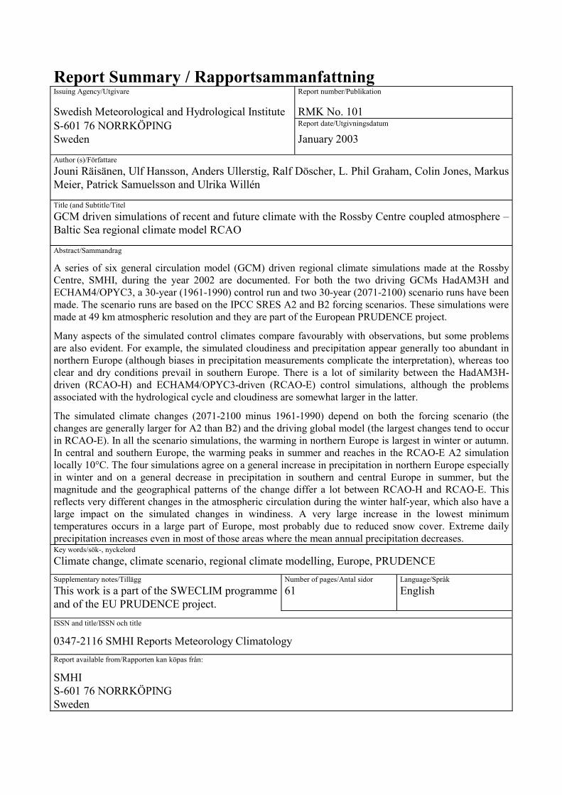
3.5.2 Extremes of wind speedAs already noted by Rummukainen et al. (1998) for the first version of the RCA model,the highest wind speeds in RCAO are relatively modest (Fig. 14). The average annualmaximum values over land are typically 9-12 m s-1, and even over the Baltic Sea windspeeds exceeding 20 m s-1 are very rare. The absolutely highest wind speed occurringover the Baltic Sea during the 30-year period is 23.5 m s-1 in RCAO-H and 25 m s-1 inRCAO-E. However, the fact the model in principle simulates mean winds for the 2400km2 grid boxes may act to smooth out the local extremes.

Figure 14. The average annual maximum 10 m wind speed (m s-1) in the RCAO-H and RCAO-Econtrol simulations.

3.6 Snow conditionsThe simulated snow conditions are illustrated in Fig. 15 with two statistics: the averageannual duration of the snow season and the average annual maximum water content ofthe snow pack. The former quantity is somewhat sensitive to the exact definition; herethe areal snow fraction predicted by RCAO2 is used (for example; a monthly meansnow fraction of 0.5 is intepreted as 15 days with snow cover). Nevertheless, theagreement with observations in Sweden (Raab and Vedin 1995, p. 94) appears good. Forthe maximum water content of the snow pack, quantitative comparison with stationobservations is done in Table 2. For most locations, the model is in good agreementwith the observations. However, the simulated values tend to be slightly too low insouthern and too high in northern Sweden. The former bias likely results from thesomewhat too warm simulated temperatures and the latter from too abundantprecipitation. The positive bias in the simulated snow maxima is particularly large attwo stations in the inland of northern Sweden (Jokkmokk and Hemavan). This is relatedto the fact that the abundant orographic precipitation, which in reality mainly falls overthe western side of the Scandinavian mountains, partly spills over to the eastern side inthe model. For improvement, higher model resolution would be needed. The differencesbetween RCAO-H and RCAO-E are relatively modest, although in southern SwedenRCAO-E tends to have somewhat more snow and a longer snow season than RCAO-H.

19

Figure 15. The average annual duration of the snow season (top) and the average yearlymaximum water content of the snow pack (bottom) in the RCAO control runs.

Table 2. Average annual maximum water content of the snow pack (mm) at selected Swedishlocations. The observations (Raab and Vedin 1995, p. 96) represent the period1968-1993, the model results the simulated years 1961-1990.

Location Latitude Longitude Observed RCAO-H RCAO-EKatterjåkk 68.7°N 18.2°E 386 419 382Jokkmokk 66.5°N 20.2°E 116 203 210Hemavan 65.8°N 15.1°E 252 472 460Haparanda 65.5°N 24.2°E 135 175 161Umeå 63.8°N 20.3°E 130 164 163Söderhamn 61.3°N 17.1°E 95 86 106Malung 60.7°N 13.7°E 107 147 156Karlstad 59.4°N 13.3°E 47 37 47Stockholm 59.4°N 18.0°E 37 29 42Göteborg 57.8°N 11.9°E 34 18 19Nässjö 57.6°N 14.7°E 72 43 54Kalmar 56.7°N 16.3°E 36 24 36Falsterbo 55.4°N 12.8°E 17 13 18

20

3.7 Other aspects of the surface hydrology

Figure 16. Evaporation (left), point runoff (middle) and fractional soil moisture (per cent of amaximum of 242 mm) in the RCAO control simulations. The first two rows show the30-year annual means in RCAO-H and RCAO-E, and the last two rows the averageseasonal cycles in Sweden and the land area south of 49°N.

The simulated precipitation (Section 3.4) and snow conditions (Section 3.6) havealready been discussed. Results related to some other aspects of the surface hydrologyare shown in Fig. 16. The first two columns display the simulated evaporation and

21

runoff generation, both scaled from the 360-day model year to a 365-day year, and thethird the total soil moisture, summed over the surface and deep soil layers and expressedin per cent of the maximum capacity of 242 mm.

In the northern parts of the model domain, evaporation is slightly larger in RCAO-Hthan in RCAO-E, despite the more abundant precipitation in the latter. The annual areamean in Sweden is 357 mm in RCAO-H and 344 mm in RCAO-E, both close to theestimate 370 mm given by Raab and Vedin (1995, p. 111). The simulated soil moisturecontent in Sweden and other parts of northern Europe is close to saturation in most ofthe year, especially in RCAO-E, and evaporation is governed more by the availability ofenergy than water. The slightly lower summer evaporation in RCAO-E in Swedenreflects larger cloudiness, which reduces the solar radiation reaching the surface.

The larger precipitation together with the slightly smaller evaporation makes runoff inSweden substantially larger in RCAO-E (606 mm per year) than in RCAO-H (514 mmper year). Both values exceed the observational estimate of Raab and Vedin (1995, p.111), 380 mm per year. For the whole Baltic Sea runoff area as well, runoff is muchlarger in RCAO-E than in RCAO-H (468 vs. 362 mm per year).

The simulated hydrological regime in the southern part of the model domain is verydifferent from that in the north. The soil is dry, especially in late summer and autumn,and evaporation is severely restricted by the lack of moisture. Most of the modest runoffoccurs in winter. Because of the negative bias in precipitation, the model most likelyunderestimates runoff generation in this area.

3.8 Ice conditions

3.8.1 Lake iceFigure 17 provides a comparison between the long-term mean observed (Eklund 1998,1999) and simulated ice conditions in a number of Swedish lakes. The observationaldata cover lakes of widely varying size but are mostly for relatively large lakes (mediumarea about 30 km2). For both the two parameters, the average ice season length and theannual maximum ice thickness, the first-order observed geographical variation iscaptured in the simulations. Lakes in southern (northern) Sweden have mild (severe) iceconditions in both the model and in nature. However, the simulated ice season is in mostlakes somewhat too short, with the ice forming too late and melting too early. Theobserved mean over the 37 lakes with data available is 170 days, and the simulatedvalues are 147 days in RCAO-H and 154 days in RCAO-E. This is qualitativelyconsistent with the relatively mild winter climate in the simulations. However, there isno systematic underestimate of the average annual maximum ice thickness. Theobserved value, averaged over 26 lakes, is 40 cm, whereas those for RCAO-H andRCAO-E are 40 and 44 cm. A similar apparent discrepancy between the simulated iceseason length and maximum ice thickness already occurred in the earlier RCA1simulations (Rummukainen et al. 2001).

22

Figure 17. Comparison between simulated and observed ice conditions in Swedish lakes. (a)The locations of the 37 lakes with observations of average ice season length (closedcircles) and 26 lakes with observations of mean annual maximum ice thickness(boxes). (b) Scatter diagram between the average observed and average simulatedice season length (open circles for RCAO-H and crosses for RCAO-E). (c) As (b)but for the mean annual maximum ice thickness.

Ice season length and especially the maximum ice thickness in RCAO-H are stronglyaffected by the problem described in Section 2.5. The results for RCAO-H in Fig. 17therefore exclude all winters when the ice thickness exceeded 1.5 m.

3.8.2 Baltic Sea ice coverFigure 18 shows the simulated 30-year time series of annual maximum ice area in theBaltic Sea including the Kattegat. As expected from the colder winters in thissimulation, there is on the average slightly more ice in RCAO-E (mean 231 × 103 km2,range from 113 × 103 km2 to 398 × 103 km2) than in RCAO-H (mean 196 × 103 km2,range from 100 × 103 km2 to 376 × 103 km2). These values are in reasonable agreementwith observations for 1961-1990 by the Finnish Marine Research Institute (mean 204 ×103 km2, range from 52 × 103 km2 to 405 × 103 km2). The simulated Baltic Sea climatewill be reported in more detail elsewhere.

Figure 18. Yearly maximum Baltic Sea ice area in the RCAO-H (solid) and RCAO-E (dashed)control runs.

23

4 Simulated climate changes for the period 2071-2100In this and the following section, the simulated climate changes, defined as differencesin climate between the scenario (2071-2100) and the control period (1961-1990) aredescribed. Altogether, the two driving global models and the two forcing scenarios givefour scenarios of regional climate change. A gallery of figures and some tables areprovided in this section to illustrate the similarities and the differences between thesescenarios. The largely descriptive approach in this section will be complemented inSection 5 by a more quantitative statistical approach.

The order of discussion in this section follows that in the previous one. The changes insea level pressure and cloudiness are discussed in the first two subsections, since theyare useful for understanding some of the other changes. It should be emphasised rightfrom the outset, however, that the largest (in comparison with natural variability)simulated change in surface climate is the general increase in temperature (Section 4.3).

4.1 Sea level pressure

4.1.1 Time mean sea level pressureMost of the interannual variability of temperature, precipitation and other aspects ofsurface climate in Europe results from variations in the atmospheric circulation.Likewise, systematic changes in the circulation with changing atmospheric compositionmight modify the changes in surface climate in an important manner, over the moredirect thermodynamic aspects of global warming. It is, however, not clear how thecirculation will respond to changes in radiative forcing. As illustrated for the time meansea level pressure in Fig. 19, the RCAO-H and RCAO-E scenario simulations give insome seasons quite different answers to this. These differences are essentially inheretedas such from the driving GCM simulations (not shown).

Beginning from the A2 minus control run climate changes, the RCAO-H experimentindicates very little annual mean pressure change, even though this results partly foropposing changes in different seasons. For example, a wintertime pressure decreasecentred over the southern Norvegian Sea is to a large extent balanced by a pressureincrease in the same area in summer and autumn. Except for summer, the pressurechanges in RCAO-H are relatively weak compared with the simulated natural variability(Section 5.1). In RCAO-E, the changes are larger and more consistent between differentseasons. In the annual mean there is a slight increase in pressure over central Europe anda strong decrease over northern Scandinavia and the Arctic Ocean. Some variant of thispattern is seen in all four seasons, although it migrates somewhat to the south in winterand to the north in summer. The pressure decrease near the northern boundary of themodel domain is largest (over 10 hPa) in winter and spring. This pattern indicates anincrease in the time-mean westerly geostrophic winds over northern Europe and thenorthern North Atlantic, and it also suggests a northward shift in cyclone activity.

24

Figure 19. Changes in seasonal and annual mean sea level pressure (differences from thecorresponding control run 30-year means) in the RCAO climate changesimulations. Contours at every 1 hPa; negative values are shaded.

The B2 simulations redproduce most of the changes in A2, although with smalleramplitude1. Some qualitative differences do occur. For example, in RCAO-H in spring,the B2 simulation indicates a slight increase in pressure over northern Scandinavia, incontrast to the slight decrease in A2. Similarly, the strong pressure decrease in RCAO-E

1 The A2 minus control and B2 minus control climate changes are not independent from each other,because the same control run has been used in defining both of them. This tends to produce some apparentsimilarity between the changes in A2 and B2 even when the statistical significance of the changes is weak.

25

in winter extends further southwest to the northern North Atlantic in the B2 than in theA2 simulation. However, some differences of this type would be expected simply fromthe substantial natural variability of the atmospheric circulation. As will be discussed inSection 5.1, any signs of real (statistically significant) nonlinearity between the climatechanges in the A2 and B2 simulations are relatively weak.

4.1.2 Band-pass filtered variabilityThe changes in synoptic time scale pressure variability are illustrated in Fig. 20 usingthe band-pass filtered standard deviation of sea level pressure. The traditional band-passfilter of Blackmon (1976) is used, which passes variations in approximately the 2.5 to 6-day period range. Results are shown only for the winter when the differences in timemean pressure change between RCAO-H and RCAO-E are greatest, and only for the A2scenario in which the changes are largest. More frequently, the 500 hPa geopotentialheight variability is analysed in this context but the choice of the level does not affectthe basic conclusions.

The strongest variability in the control runs occurs over the northwestern AtlanticOcean, from where a reasonably well-defined “storm track” extends towards northernEurope and the Arctic Ocean. In the A2 scenario run, the area of large variabilityextends further eastward in both RCAO-H and RCAO-E, but the change is larger inRCAO-E. In addition, the increase in variability in RCAO-H occurs mainly on thesouthern side of the control run storm track, whereas the pattern in RCAO-E representsa more direct eastward or northeastward extension of variability. These differencesbetween the two experiments are largely as expected from the differences in the wintertime mean pressure change in Fig. 19.

Figure 20. The band-pass filtered standard deviation of sea level pressure in December-February in the RCAO-H and RCAO-E control runs (contours at every 0.5 hPa) andthe change in this from the control run to the A2 scenario run (shading).

The band-pass filtered variability measures the combined effect of transient cyclonesand anticyclones but is unable to separate between these. The time mean pressurechanges in Fig. 19 suggest that the cyclones in RCAO-E become more frequent orintense especially over the northern flank of the area where the variability increases,whereas anticyclonic activity primarily increases over the southern flank of this area.

26

4.2 Total cloudinessClouds and their interaction with radiation are probably the single most importantsource of uncertainty in the magnitude of greenhouse-gas-induced global mean warming(Stocker et al. 2001). Changes in cloudiness might also have important effects onregional climates, but it is important to remember that the impact of clouds ontemperature is twofold. By reflecting sunlight clouds act to cool the surface especially insummer and during the daylight hours, but by absorbing terrestrial long-wave radiationthey also act to warm the surface. The net cloud feedback on temperature changestherefore depends, in addition to the change in the total cloud cover, on the diurnal cycleof the change and the time of the year, on the height in the atmosphere where cloudinessincreases or decreases, and on other possible changes in cloud properties.

Figure 21. Changes in December-Febaruary, June-August and annual mean cloud cover (inper cent of full sky) in the RCAO climate change simulations. The colour scale isgiven below the figure.

Figure 21 shows the RCAO-simulated changes in average cloud cover in winter,summer and the annual mean (the changes in spring and autumn are generally betweenthose in winter and summer). The changes in the A2 and B2 scenario runs tend to be ofthe same sign, but the magnitude of the changes is larger in A2 than in B2. In winter,cloudiness increases slightly in most of northern Europe in both RCAO-H A2 and B2. InRCAO-E, the increase is less widespread, being largest at the west coast of Norway,where the increased westerly flow indicated by the change in the time mean sea levelpressure (Fig. 19) leads to increased orographic uplift of air. The decrease in cloudiness

27

on the eastern side of the Scandinavian mountains especially in RCAO-E A2 also mostlikely results from the stronger westerly flow. Further south, in the Mediterranean area,the RCAO-H and RCAO-E experiments both indicate a general decrease in cloudiness,although with substantial differences in the patterns of change.

The changes in summer are dominated by a large reduction in cloud cover over centralEurope, especially its western parts. The largest changes occur in RCAO-E A2, in whichsummer mean cloud cover locally decreases by 24% (of full sky) in France. Part of thisdecrease may be explained by changes in atmospheric circulation: the increase in timemean easterly flow indicated by the pattern of pressure change in all four scenario runssuggests suppressed moisture supply from the Atlantic Ocean to western and centralEurope. However, local thermodynamic feedbacks between reduced precipitation, soilmoisture and evaporation (Sections 4.4 and 4.7) might play an even more importantrole. Smaller reductions in cloudiness extend southward to the Mediterranean area andnorthward to southern Scandinavia. Even further north and at the west coast of Norwaysummer cloudiness increases, especially in the two RCAO-E simulations. The smallerdecrease in cloudiness in the Mediterranean area than in central Europe may result atleast partly from the fact that the summer mean cloudiness in the Mediterranean regionis very low even in the control simulations.

The annual mean total cloudiness decreases in most of the model domain in all fourscenario simulations, excluding some parts of northern Europe.

4.3 Surface air temperature

4.3.1 Time mean temperatureMaps of seasonal and annual mean surface air temperature change in the RCAOexperiments are shown in Fig. 22. These reveal several features of interest:

� For both the A2 and the B2 scenarios, the warming is in most areas and seasonslarger in RCAO-E than in RCAO-H.

� The maximum annual mean warming occurs in central and southern rather thannorthern Europe, at least excluding RCAO-H B2.

� In northern Europe, the warming is largest in autumn and winter, as is commonlythe case even in global climate models (Räisänen 2000). However, the warmingin winter is distinctly larger in RCAO-E than in RCAO-H. This results, at leastin part, from the increase in westerly winds in RCAO-E and the absence of suchan increase in RCAO-H.

� The warming over the Atlantic Ocean, which is dictated by the SST change inthe driving global model, is much larger in RCAO-E than in RCAO-H. This maybe related to different changes in the Atlantic thermohaline circulation. InECHAM4/OPYC3, there is no change in the strength of this circulation withincreasing greenhouse gas forcing (Latif et. al 2000), whereas HadCM3simulates a roughly 20% decrease in circulation strength in both the A2 and B2scenario runs by 2100 (http://www.meteoffice.gov.uk/research/hadleycentre/pubs/brochures/B2000/predictions.html). These differences in the SST changeprobably also explain some part of the difference in warming over Europe.

28

Figure 22. Changes in seasonal and annual mean surface air temperature (differences from thecorresponding control run 30-year means) in the RCAO climate changesimulations. Contours and shading at every 1°C.

� In southern and central Europe, the warming peaks in summer. In RCAO-E, inparticular, the warming in southwestern Europe is extremely large, with amaximum of over 10°C in France in the A2 scenario and 7°C even in the B2scenario. This very large warming is accompanied by substantially reducedcloudiness (Section 4.2), precipitation (Section 4.4), and soil moisture (Section4.7). These changes most probably reinforce each other via the feedback loopdescribed by Wetherald and Manabe (1995). However, as noted for cloudiness inSection 4.2, changes in atmospheric circulation may also play a role.

29

� It is not quite clear why the summertime warming in central and southwesternEurope is so much larger in RCAO-E than in RCAO-H, especially as thechanges in the pressure pattern (Fig. 19) in this season are similar. One factorthat likely plays a role are different changes in the atmospheric circulation inspring. The RCAO-E simulations show a centre of increasing MAM mean sealevel pressure over central Europe, whereas the pattern in the RCAO-Hsimulations is relatively diffuse. This leads to a substantial decrease in springcloudiness (not shown) and precipitation (Section 4.4.1) over central andsouthwestern Europe in RCAO-E, in contrast with relatively small changes inRCAO-H. Consequently, the soil dries out earlier and more severely in RCAO-Ethan in RCAO-H (Section 4.7).

� The temperature changes over the Baltic Sea are largely determined by the SSTand sea ice changes simulated by the RCO model, and they occasionally differfrom the temperature changes in the surrounding land areas. In particular, the air(and surface water) over the southern and central parts of the Baltic Sea warmsmore in summer than the air over nearby land areas, especially in the RCAO-Hsimulations. On the other hand, a local minimum of warming occurs over thenorthern Bothnian Bay in RCAO-E. The dynamics of these sea-land differencesstill need to be investigated. Possible causes might include changes in the BalticSea ocean circulation and temperature stratification.

� The A2 and B2 scenario simulations give qualitatively very similar results,although the magnitude of the warming is smaller in B2 than in A2. It is also ofinterest to note that the annual mean warming is in most of the domain verysimilar between RCAO-H A2 and RCAO-E B2.

4.3.2 Interannual variability of monthly mean temperaturesThe time-averaged warming is accompanied in the RCAO simulations by a decrease ininterannual temperature variability in northern Europe in winter (see Figs. 23e-f forresults for Sweden), with a larger change in RCAO-E than in RCAO-H. In summer,variability changes little in northern Europe but tends to increase further south (Figs.23g-h). The seasonal and geographical details of the change vary a lot between the A2and B2 scenarios, probably because these changes have a relatively low signal-to-noiseratio. For example, the RCAO-H B2 simulation shows an area of increased annuallyaveraged variability in eastern Europe that is absent in RCAO-H A2 (Figs. 23a,c).

A tendency towards reduced mid- and high-latitude temperature variability in winter in awarmer climate also occurs in global climate models, most likely due to a reduction ofsnow and ice (Räisänen 2002). A slight increase in midlatitude temperature variabilityin summer is likewise a common model result, which probably reflects reduced soilmoisture. When the soil becomes sufficiently dry, the capability of evaporation to coolthe surface decreases. This acts to increase both the average summer temperatures andtheir interannual variability, because the lack of evaporative cooling has its largest effectin those summers when the atmospheric circulation favours warm conditions and, withsufficient soil moisture, large evaporation (Delworth and Manabe 1988, 1989; Tett et al.1997).

30

Figure 23. Top: Changes in the 12-month mean interannual standard deviation of monthlymean temperature (per cent differences from the corresponding control run 12-month means). Bottom: the seasonal cycles of the area mean of the standarddeviation (in °C) in Sweden and in the land area south of 49°N. Both the control runand the scenario run temperature series were detrended before the calculation ofthe standard deviations to remove any biases associated with the gradual change inforcing. In this and the following figure only land areas are shown, becausetemperature varies much less over sea than over land.

4.3.3 Diurnal temperature rangeThe changes in the average diurnal temperature range (Fig. 24) show some resemblancewith the changes in interannual variability. The annual mean diurnal range decreases innorthern Europe, locally by over 25% in the RCAO-E A2 simulation. Further south thevariability increases, with the largest relative increase in those parts of southwesternEurope (in particular France) where the decrease in cloudiness is largest. However, themagnitude of the change varies substantially between the four scenario simulations.

In the southern half of the model area as a whole (Fig. 24g-h), the diurnal temperaturerange increases slightly in most of the year. In Sweden (Fig. 24e-f) and in northernEurope in general, the decrease in variability is largest from late autumn to spring. Thedecrease in snow cover (Section 4.6), which prevents temperature from falling to verylow levels in clear nights, is a main suspect for this. It should be noted, though, thatregular night-to-day temperature variability in northern Europe in midwinter is weak.The diurnal temperature range and changes in this between different model runs aretherefore also affected by irregular day-to-day temperature variations (see Räisänen etal. 1999).

31

Figure 24. Top: changes in the 30-year annual mean diurnal temperature range (in per cent ofthe corresponding control run 30-year means). Bottom: the seasonal cycles of theaverage diurnal temperature range (in °C) in Sweden and in the land area south of49ºN.

4.3.4 Temperature extremes

Figure 25. Changes in average yearly temperature extremes from the control runs to the A2and B2 scenario runs. The colour scale is given below the figure. Contours aredrawn at 3, 6, 10 and 15°C only

The control run average yearly temperature extremes were shown in Fig. 8. Figure 25shows the changes in these in the A2 and B2 scenario runs. In northern Europe, theincrease in yearly maximum temperatures is broadly the same as that in the June-July-August mean temperature (Fig. 22). Further south, the warm extremes generally increase

32

more than the mean temperature, even though the summer time mean warming is alsovery large. In France in RCAO-E A2, the highest yearly maximum temperaturesincrease by up to 12°C. This is consitent with the increased interannual and diurnaltemperature variability discussed in the previous subsections. The lowest winter minimum temperatures increase in most of Europe much more thanthe December-February mean temperature (the lower half of Fig. 25 and the first row ofFig. 22). The largest changes occur in southern Scandinavia and central-eastern Europe,where the increase exceeds 15°C in RCAO-E A2. This corresponds to the areas where amore or less significant snow cover occurs in the control runs but which become almostsnow-free in the scenario runs (Section 4.6). In southwestern Europe, which is snow-free even in the control runs, the change in the lowest winter temperatures is moremodest. Even in northern Scandinavia, where a good deal of snow remains even in thescenario runs, the changes in the lowest minimum temperatures tend to be somewhatsmaller than those in eastern and central Europe.

For the sake of curiosity, Table 3 lists some statistics of absolute geographicaltemperature extremes (i.e., highest and lowest temperatures occurring somewhere withina given geographical area). Although the temperature never reaches 40°C in Sweden inany of the scenario runs, the absolutely highest temperatures near the southern edge ofthe map domain (in northern Africa) are well above the current world record of 56.7°C.As far north as in the southern Netherlands, temperature once exceeds 50°C in RCAO-EA2. Looking at the other end of the distribution, severe cold occasionally occurs in thenorthernmost parts of the model domain even in the scenario runs, but the differencefrom the control run values is nevertheless quite large.

Table 3. Absolute temperature extremes (°C) in the RCAO simulations. The values forSweden give the absolutely highest or lowest temperatures occurring in any gridbox in Sweden in an average year (rows 1 and 4) or once in the 30-year simulations(rows 2 and 5). Rows 3 and 6 show the absolute 30-year extremes for the whole mapdomain.

RCAO-H RCAO-E CTRL A2 B2 CTRL A2 B2yearly maximum, Sweden 28.9 33.1 30.9 26.4 32.1 29.530-year maximum, Sweden 33.8 38.9 35.0 30.7 38.4 35.930-year maximum, all points 57.0 61.5 59.0 54.5 61.4 60.8yearly minimum, Sweden -47.4 -37.9 -39.5 -47.2 -37.9 -39.630-year minimum, Sweden -56.0 -45.9 -49.4 -55.6 -44.2 -49.630-year minimum, all points -65.0 -49.5 -56.7 -60.8 -46.7 -50.7

4.4 Precipitation

4.4.1 Time mean precipitationThe changes in the 30-year seasonal and annual mean precipitation, expressed in percent of the control run values, are shown in Fig. 26. There are large geographical and

33

seasonal variations in the change, and also some substantial differences between theHadAM3H- and ECHAM4-driven simulations. The main features include the following:

Figure 26. Changes in seasonal and annual mean precipitation (per cent differences from thecorresponding control run 30-year means) in the RCAO climate changesimulations. The colour scale is given below the figure. Contours are drawn atevery 30% only. A slight smoothing is applied for legibility.

� All four scenario simulations agree on a general increase in precipitation innorthern and central Europe in winter. They also agree on a general and in someareas very large (up to 70% in the A2 scenario runs) decrease in summer

34

precipitation in southern and central Europe. A smaller decrease in summerprecipitation extends up to central Scandinavia in the north. Thus, the changes innorthern and central Europe have a very pronounced seasonal cycle.

� The mean annual precipitation increases in northern Europe and decreasesfurther south, except for RCAO-H B2 in which an increase occurs even in muchof southeastern Europe. However, this north-south contrast is stronger in theRCAO-E than in the RCAO-H simulations. This reflects most probably thenorthward shift in cyclone activity in RCAO-E that is absent in RCAO-H(Section 4.1).

� At the west coast of Norway, where precipitation is strongly governed by winddirection, the differences between RCAO-H and RCAO-E are huge. Theincrease in westerly winds leads to a large increase in annual precipitation inRCAO-E (up to 70% in the A2 and over 40% even in the B2 scenario run),whereas the increase in RCAO-H A2 and B2 is only 0-10%. In winter, when thetime mean westerly wind decreases in the RCAO-H scenario simulations,precipitation in northwestern Norway decreases in them. As the control run (andobserved) precipitation in western Norway is very large, these differences areeven more dramatic in absolute terms.

� The changes in the B2 simulations are in most cases qualitatively similar to butsmaller than those in the A2 simulations. However, some exceptions occur. Oneof the most notable is the contrast between decreasing annual precipitation insoutheastern Europe in RCAO-H A2 and increasing precipitation in B2.Similarly, the increase in annual precipitation extends slightly further south inRCAO-E B2 than RCAO-E A2. However, the unforced variability ofprecipitation is large and is likely to explain a substantial part of these apparentdiscrepancies (Section 5.1)

4.4.2 Interannual variability of monthly precipitationThe top row of Fig. 27 shows the per cent changes in the 12-month mean of theinterannual standard deviation of monthly precipitation. The patterns are noisy andhighly variable between the different scenario runs, but the general picture is one ofincreasing standard deviation in northern Europe and decreasing standard deviation insouthern Europe. Thus, as the first approximation, the changes in the absolute amplitudeof interannual precipitation variability tend to follow those in the mean precipitation (cf.Fig. 26). This behaviour has been documented well in earlier studies (e.g., Räisänen2002) and is qualitatively expected since precipitation is bounded from below by zero.

A more interesting question is if there is any systematic difference between the per centchanges in the standard deviation and the mean (i.e., does the coefficient of variation ofprecipitation change). This is addressed in the lower half of Fig. 27 by comparing theseasonal cycles of the changes in the mean and the standard deviation in Sweden and inthe land area south of 49°N. In Sweden, the two changes tend to follow each other, butin winter all four scenario runs show a smaller increase in the standard deviation than inthe mean (excluding RCAO-E B2 in February). This difference is particularlypronounced in RCAO-E A2. South of 49°N, the situation is reversed, with the meanprecipitation decreasing in most months more than the standard deviation (mostregularly so in RCAO-E A2). This implies that, in the southern parts of the model area,the low extremes of monthly precipitation decrease by an even larger per cent fractionthan the mean precipitation, while the high extremes decrease less.

35

Figure 27. Top: Changes (per cent differences from the control run values) in the 12-monthmean interannual standard deviation of monthly precipitation. Bottom: per centchanges in the area means of the standard deviation (solid lines) and the time meanprecipitation (dashed lines) in Sweden and the land area south of 49ºN.

All other factors being the same, the coefficient of variation of monthly precipitationincreases with decreasing number of precipitation days (Räisänen 2002). Thus, onewould expect from these results a decrease in the number of precipitation days in thesourthern part of the model area and an increase in the north, with the largest changes inRCAO-E A2. This is actually the case.

4.4.3 Number of precipitation days The simulated changes in the annual number of days with at least light (≥ 0.1 mm), atleast moderate (≥ 1.0 mm) and heavy precipitation (≥ 10 mm) are shown in Fig. 28.Using the lowest threshold, the number of precipitation days increases in northernEurope excluding southern Scandinavia, and decreases in southern and central Europe.These changes are larger for the A2 than the B2 scenario, and in RCAO-E than RCAO-H. Thus, in northern Europe, completely dry days that are infrequent even in the controlruns become on an annual basis even less common in the scenario runs. Further south,the number of dry days increases. The results for the 1.0 mm threshold are similar.Using either of these two thresholds, the decrease in the number of precipitation daysextends further north than the decrease in annual precipitation (Fig. 26).

The number of days with heavy (≥ 10 mm) precipitation also increases in northernEurope and decreases in most of southern Europe excluding RCAO-H B2, but the areaof increase extends further south than in the case of the first two thresholds. The largestabsolute increases and decreases occur, as expected, in those mountain areas whereheavy precipitation is most frequent in the control simulations.

36

Figure 28. Changes (A2 or B2 scenario run minus control run) in the average annual numberof days with at least 0.1 mm (top), 1 mm (middle) and 10 mm (bottom) ofprecipitation. The colour scale differs between the first two rows and the last row.

Table 4. Area mean changes in the number of days with precipitation exceeding varyingthresholds (from 0.1 to 20 mm). Values are given in absolute units (days per year)and in per cent (in parentheses). Results are shown for Sweden and for the landarea south of 49ºN.

P (mm) RCA-H, A2 RCA-E, A2 RCA-H, B2 RCA-E, B2Sweden ≥ 0.1 2.1 ( 1%) 10.8 ( 4%) 2.4 ( 1%) 8.6 ( 3%)

≥ 1.0 7.6 ( 4%) 19.0 ( 11%) 3.9 ( 2%) 14.5 ( 8%) ≥ 5.0 8.2 ( 15%) 16.6 ( 27%) 5.5 ( 10%) 12.0 ( 19%)≥ 10 4.5 ( 28%) 9.6 ( 49%) 3.3 ( 20%) 7.0 ( 36%)≥ 20 0.8 ( 42%) 1.9 ( 79%) 0.6 ( 29%) 1.3 ( 57%)

< 49°N ≥ 0.1 -21.7 (-14%) -30.1 (-20%) -11.6 (-14%) -16.5 (-11%) ≥ 1.0 -13.7 (-15%) -22.0 (-24%) -6.4 (-15%) -11.8 (-13%) ≥ 5.0 -5.2 (-13%) -9.5 (-26%) -1.6 (-13%) -4.4 (-12%)≥ 10 -1.7 (-10%) -3.6 (-21%) 0.1 (-10%) -1.2 ( -7%)≥ 20 0.1 ( 2%) -0.3 ( -6%) 0.5 ( 12%) 0.3 ( 7%)

Table 4 gives the area mean changes in the number of precipitation days for variouslower thresholds for Sweden and the land area south of 49°N. Here, both absolute (daysper year) and relative (per cent of the control run mean) changes are given. The higher

37

the threshold used, the larger is the relative increase in the number of days withprecipitation above that threshold in Sweden and elsewhere in northern Europe. In thissense there is an “unproportional” increase in the number of very wet days in northernEurope, even though this does not imply that the magnitude of the extremes wouldincrease more than the mean precipitation (Section 4.4.4). In the land area south of 49°Nthe total number of precipitation days decreases substantially, but the decrease is muchsmaller or reversed to an increase for the highest threshold (20 mm) used.

4.4.4 Extreme daily precipitationFigure 29 shows the simulated changes in the 30-year mean yearly maximum one-dayprecipitation. The patterns of change are very noisy, but all four scenario runs indicatean overall increase in the yearly extremes even in those parts of southern and centralEurope where the mean annual precipitation decreases. Very similar results werereported by Räisänen and Joelsson (2001) for the previous Rossby Centre regionalclimate change simulations made with the RCA1 model. In that paper it was also shownthat, although the changes in individual grid boxes were very heavily affected byinternal variability, the statistical significance of the changes increased dramaticallywhen they were averaged over a sufficiently large area. Table 5 compares the changes inthe area means of mean annual precipitation and the yearly maximum one-dayprecipitation in two areas, Sweden and all land south of 49°N. Also included in thiscomparison are the area means of the absolutely largest one-day precipitation occurringwithin the whole 30-year simulations.

Figure 29. Per cent changes in the 30-year means of yearly maximum one-day precipitationfrom the control runs to the A2 and B2 scenario runs. The colour scale is givenbelow the figure. Contours are omitted except for 0%.

In an area mean sense, the average yearly and 30-year precipitation extremes increase inboth two areas and all four scenario runs. There is a tendency for the 30-year extremesto increase more (even in per cent terms) than the yearly extremes, but this is not thecase for the two B2 simulations in Sweden. The increases in the extremes are by andlarge similar between the two areas, although the changes in the mean precipitation arenot. All four scenario runs show a decrease of time and area mean precipitation in thearea south of 49°N but an increase in Sweden (which is in RCAO-E A2 and B2 largerthan the increase in extremes). These apparently contradictory results are consistent withthe different changes in the number of precipitation days in these areas. In Sweden, boththe intensity and (especially in RCAO-E) annual number of precipitation eventsincrease, which leads to a relatively large increase in the time mean precipitation. In the

38

southern parts of the model domain, any increases in precipitation intensity are morethan compensated by a decrease in the number of precipitation days.

Table 5. Per cent changes in the area means of mean annual precipitation (rows 1 and 4),the average yearly maximum one-day precipitation (rows 2 and 5) and the absolute(30-year) maximum daily precipitation (rows 3 and 6). Results are shown forSweden and for the land area south of 49°N.

RCA-H, A2 RCA-E, A2 RCA-H, B2 RCA-E, B2Sweden Mean 12 23 8 17

Max (1 yr) 13 14 7 11Max (30 yr) 23 15 6 9

< 49°N Mean -11 -21 -2 -9Max (1 yr) 8 7 9 9Max (30 yr) 16 19 12 14

4.5 Wind speed

4.5.1 Time mean wind speedAs expected from the different changes in mean sea level pressure and transient activity(Section 4.1), the changes in the average 10 m wind speed differ substantially betweenthe RCAO-H and RCAO-E experiments. In the annual mean (upper row of Fig. 30), thechanges in the two RCAO-H scenario runs are very modest (within ±4% in virtually thewhole of Europe). In RCAO-E, larger changes occur. Wind speeds increase in northernEurope, in the Nordic area typically by about 8% in RCAO-E A2, and decrease in theMediterranean region. As shown in the lower half of Fig. 30, the increase in Sweden(and in northern Europe in general) is largest in winter and early spring, when theincrease in the north-south pressure gradient in RCAO-E is largest (Fig. 19). Thedecrease in the southern half of the model domain is more seasonally uniform but occursmainly in the summer half-year.

Figure 30g shows the seasonal cycles of the change over the Baltic Sea, where thesimulated wind changes are substantially modified by stability effects associated withchanges in SST and ice cover. In winter, the mean wind speed in RCAO-E increaseseven more over the Baltic Sea than over the surrounding land areas, with the largestincrease over the central and northern parts that have a decent ice cover in the controlruns but lose most of it in the scenario runs (Section 4.8). Most probably for the samereason a small increase occurs in winter even in RCAO-H, although there is nosystematic change in the surrounding land areas. In summer the difference betweenRCAO-H and RCAO-E is reversed, with more positive changes in RCAO-H than inRCAO-E. The increase in summer windiness over the Baltic Sea in RCAO-H apparentlyreflects the large increase in Baltic Sea SSTs in this experiment, which is revealed bythe pronounced land-sea contrast in warming in Fig. 22 and leads to reduced surfacelayer stability.

39

Figure 30. Top: changes in the 30-year annual mean wind speed (per cent differences from thecorresponding control run 30-year means). Bottom: the seasonal cycles of thechange in Sweden, the land area south of 49º, and the Baltic Sea (see the panel forSweden for the identification of the different simulations).

4.5.2 Extremes of wind speedThe changes in the average yearly maximum wind speed (Fig. 31) tend to follow thechanges in the time mean wind speed. The changes in the two RCAO-H scenario runsare generally small, whereas the RCAO-E simulations indicate a general increase inwind extremes in northern Europe. Similar conclusions hold for the absolute 30-yearextremes of wind speed (not shown).

Figure 31. Per cent changes in the average yearly maximum wind speed from the RCAOcontrol runs to the A2 and B2 scenario runs. Contours and shading at every 4%.

4.6 Snow conditionsThe warming in the RCAO scenario runs leads to a substantial shortening of the snowseason (upper row of Fig. 32). Following the magnitude of the warming, the decrease inthe snow season length is larger in the A2 than in the B2 simulations, and larger inRCAO-E than in RCAO-H. However, the largest changes (from 45 to over 90 days

40

depending of the simulation) occur in all cases in the same areas: in a belt extendingfrom central Scandinavia to the Baltic states, at the west coast of Norway and over theAlps. These areas have a comparably decent snow season in the control runs but aremilder and therefore more sensitive to temperature increase than northern Scandinavia,where the decrease in snow season length is smaller. In areas like southernmostScandinavia and central Europe where the snow season is short even in the control runs,the decrease in the snow season length is also smaller in absolute terms but large inrelative terms. For example, those parts of southwestern Sweden that have 30-60 snowdays in the control runs become almost snow-free (less than 10 snow-covered days) inboth the two A2 scenario runs (not shown).

The lower row of Fig. 32 shows the changes in the average yearly maximum snow waterequivalent. The magnitude of the changes depends on the simulation but the largest percent decreases from the control run values occur in those areas that had relatively littlesnow even in the control simulations. In northern Finland and over the Scandinavianmountains, the change is relatively small but still negative. This might appearsurprising: given the large simulated increases in winter precipitation and the fact thatthe winter mean temperature remains in these areas well below zero even in the scenarioruns, one would expect the amount of snowfall to increase. This is actually the case inthe midwinter (December-February) in most of these areas, excluding the southern partsof the Scandinavian mountains in RCAO-E A2 (not shown). However, the increase inmidwinter snowfall is more than compensated by less snowfall in early and late winter,and by more frequent melting episodes.

Figure 32. Top: the change in the average duration of the snow season from the RCAO controlruns to the A2 and B2 scenario runs (in days). Bottom: the change in the averageannual maximum water content of the snow pack (in per cent of the control runmean).

41

4.7 Other aspects of the surface hydrologyIn this subsection we describe the changes in the three hydrological parameters whosecontrol run behaviour was documented in Section 3.7: evaporation, runoff generationand soil moisture.

4.7.1 EvaporationThe simulated annual mean evaporation increases in northern Europe and most ofcentral Europe in all four scenario runs (upper row of Fig. 33). The changes are largestin the A2 scenario runs, in which the annual increase in the Nordic area is about 20%.Even larger changes occur locally over the Scandinavian mountains. As illustrated inFig. 33e-f for Sweden, evaporation increases in northern Europe in all seasons.However, the increase is in relative terms largest in winter and spring, especially inRCAO-E. This differs from the earlier RCA1 experiments in which evaporationdecreased in winter (section 5.3). This difference is thought to be explained by thechanges in the land surface scheme documented in Bringfelt et al. (2001), which act toreduce evaporation over snow-covered surfaces to more realistic levels. As there is moresnow in the control than in the scenario runs, this tends to increase the scenario runminus control run differences in evaporation. In late summer, the simulated increases inSweden mean evaporation are relatively small, probably because a decrease of soilmoisture (Section 4.7.3) acts to suppress evaporation in the southern parts of thecountry.

Figure 33. Top: changes in the 30-year mean annual evaporation (per cent differences fromthe corresponding control run 30-year means) in the A2 and B2 scenario runs.Bottom: the average seasonal cycles of evaporation in Sweden and in the land areasouth of 49ºN. The black, red and blue lines give the results for the control, A2 andB2 runs, respectively.

In much of southern Europe, the simulated decreases in precipitation also lead to adecrease in annual evaporation. In all four scenario runs evaporation generally increases

42

in this area in winter and early spring, but decreases in summer and autumn (Fig. 33g-h)because of a marked decrease in soil moisture (Section 4.7.3). The decrease inevaporation leaves more radiation energy to drive the sensible heat flux, contributing inthis way to the large increase in summer temperatures.

Over the northern North Atlantic, evaporation is reduced substantially in RCAO-H. Inthis experiment, wind speeds over the northern North Atlantic decrease (Section 4.5)and the increase in SSTs is small compared with the warming of the air that is advectedfrom the surrounding continents. In RCAO-E, in which the average wind speedsincrease and the increase in SSTs is larger, the changes in evaporation over the northernNorth Atlantic are small.

4.7.2 Runoff generationThe changes in the 30-year annual mean runoff generation (Fig. 34) are determined bythe changes in precipitation and evaporation. In most of northern Europe, the annualrunoff generation increases in all four scenario runs. In RCAO-E A2 and B2, in whichthe per cent increase in precipitation is larger than that in evaporation, the per centincrease in runoff generation exceeds the increase in precipitation. In RCAO-H,precipitation increases in absolute terms more but in relative terms less thanevaporation. Consequently, runoff generation increases, but in per cent terms less thanprecipitation. Further south in central and southern Europe, and even in parts ofsouthern Scandinavia, annual runoff generation decreases. An exception is southeasternEurope in RCAO-H B2, where, however, the control run runoff is low so that the largerelative increase is relatively modest in absolute terms.

Figure 34. Top: changes in the 30-year mean annual runoff generation (per cent differencesfrom the corresponding control run 30-year means). Bottom: the average seasonalcycles of runoff generation in Sweden and in the land area south of 49ºN. The black,red and blue lines give the results for the control, A2 and B2 runs, respectively.

43

The seasonal cycle of runoff generation is affected by changes in snow conditions andsoil moisture, as well as precipitation and evaporation (see the lower half of Fig. 34 forresults for Sweden and for the land area south of 49°N). In Sweden, the earliersnowmelt gives an earlier spring peak in runoff generation in all four scenario runs.Increased precipitation and snowmelt during the late autumn and winter leads to asubstantial increase in runoff generation in these seasons, most notably in the RCAO-Escenario runs. Conversely, the earlier snowmelt together with reduced summerprecipitation and increased evaporation leads to a decrease in runoff generation insummer. In the area south of 49°N, the area mean runoff generation decreases almostthroughout the year, at least excluding the midwinter and (in RCAO-H B2) early spring.

4.7.3 Soil moistureOn an annual mean basis, soil moisture decreases in most of Europe in all four scenarioruns (upper row of Fig. 35), the main exception being northern Scandinavia and Russiain RCAO-E A2 and B2. The decrease is in absolute terms largest in central andsouthwestern Europe, and it is generally largest in the RCAO-E A2 simulation. Furthersouth, the decrease in soil moisture is limited by the fact that the soil is very dry even inthe control simulations.

Figure 35. Top: changes in the 30-year annual mean soil moisture (in per cent of a maximumof 242 mm). Bottom: the average seasonal cycles of soil moisture (per cent of 242mm) in Sweden and in the land area south of 49ºN. The black, red and blue linesgive the results for the control, A2 and B2 runs, respectively.

The average seasonal cycles of soil moisture in Sweden and the land area south of 49°Nare shown in the lower part of Fig. 35. In Sweden, little change occurs in winter, whenthe soil is very wet in all the simulations. However, the seasonal decrease in soilmoisture toward late summer is larger in the scenario runs than in the control runs, dueto the earlier snowmelt, increased evaporation and reduced summer precipitation. Southof 49°N, the area mean soil moisture is reduced throughout the year, but the most

44

remarkable feature is the extreme dryness of the soil in late summer. In RCA-E A2, theAugust mean for this large area is only 5% of the maximum.

4.8 Ice conditions

4.8.1 Lake ice

Figure 36. Comparison of ice conditions in Swedish lakes in the control, A2 and B2simulations, using the same sets of lakes as in Fig. 17. Top: scatter plots of theaverage duration of the ice season in 37 lakes in RCAO-H (left) and RCAO-E(right). The horizontal axis gives the ice season length in the control run and thevertical axis that in the A2 (open circles) and B2 (crosses) scenario runs. Bottom:the same for average yearly maximum ice thickness in 26 lakes.

The changes in the simulated ice conditions in Swedish lakes are illustrated in Fig. 36(see the figure caption for details). For the set of 37 lakes studied, the decrease in theaverage ice season length varies from 38 days in RCAO-H B2 to 68 days in RCAO-EA2. The decrease tends to be largest for the lakes in southern Sweden, where the wintersare relatively mild even in the control simulations. In RCAO-E A2, in particular, manylakes in southern Sweden become virtually ice-free. Further north, where the control runwinters are colder, the ice season length is reduced less even though the increase inwinter temperatures is at least as large (Fig. 22). Similar conclusions apply to thechanges in the average winter maximum ice thickness (lower part of Fig. 36). In manylakes in southern Sweden, no or only very thin ice develops in an average winter inRCAO-E A2, and this is the case to some extent even in the other simulations. Further

45

north ice thickness is also reduced substantially, but in the northernmost Swedenrelatively thick lake ice still develops in all four scenario runs.

4.8.2 Baltic Sea ice cover

Figure 37. Yearly maximum Baltic Sea ice area in the RCAO-H (solid) and RCAO-E (dashed)A2 and B2 scenario runs. Note that the scale differs from Fig.18.

Figure 38. Average annual number of days with ice cover in the Baltic Sea. Top left, middleand right: RCAO-H CTRL, A2 and B2. Bottom left, middle and right: RCAO-ECTRL, A2 and B2.

The simulated warming also leads to a large decrease in the Baltic Sea ice extent (Figs.37 and 38). Excluding the first winter which may still be affected by the initial spin-up,

46

the yearly maximum ice extent in RCAO-H A2 varies from 13 × 103 km2 to 134 × 103

km2 with a mean of 67 × 103 km2, and that in RCAO-E A2 from 15 × 103 km2 to 104 ×103 km2 with a mean of 46 × 103 km. For RCAO-H B2 the range is from from 27 × 103

km2 to 190 × 103 km2 with a mean of 91 × 103 km2, and for RCAO-E B2 from 17 × 103

km2 to 172 × 103 km2 with a mean of 76 × 103 km2. In comparison with the controlsimulations (Section 3.8.2), the average maximum ice extent decreases by 54-80%,depending on the driving model and the forcing scenario. Some ice still forms in everywinter, but even in the coldest winters in the B2 simulations the ice extent remainssomewhat below the control run mean.

As shown by Fig. 38, the ice cover in the scenario runs is largely limited to the Gulf ofFinland and the Bothnian Bay. In the northernmost Bothnian Bay, the average ice seasonlength nevertheless exceeds four months in all four scenario runs.

5 Statistical analysis of simulated climate changesThis section is devoted to statistical tables characterising the simulated climate changes.In the first subsection (5.1), the statistical significance of the simulated changes andtheir magnitude relative to the simulated interal climate variability is addressed. InSection 5.2, the agreement between the HadAM3H- and ECHAM4-driven simulationsis quantified and the contribution of internal variability to the differences between thesesimulations is estimated. Finally, because it is anticipated that these experiments will beused most actively within the Swedish climate change community, a table of Swedenarea mean climate changes is given in Section 5.3. In this subsection some comparisonis also made with the previous generation of Rossby Centre climate change simulationsdiscussed by Räisänen et al. (2000a) and Räisänen and Joelsson (2001).

5.1 Simulated changes versus internal variabilityClimate varies even under constant external conditions, both in the real world and inmodels. Any simulated climate change (computed as the difference between theclimates in two different model runs) is therefore a combination of two parts: areproducible signal associated with the external forcing, and noise associated withinternal (i.e., unforced) variability. These two parts could be separated, in principle, bymaking a large ensemble of climate change simulations with the same external forcingbut different initial conditions (in the case of regional climate change experiments, theinitial conditions would need to be varied even in the driving global model). In thatcase, the ensemble mean climate change would approach the reproducible signal withincreasing ensemble size. Without such ensembles, there is no exact way to separatebetween the signal and the noise. However, the magnitude of the simulated climatechanges can still be compared with the magnitude of noise expected from statisticalconsiderations.

A frequently used tool in this context is the t statistics, which is of the general form

)( XVXt�

�� (2)

47

Here, �X is the simulated change (e.g., 30-year annual or seasonal mean differencebetween two model runs) in variable X and V(�X) is the error variance of the simulatedchange. If the values of X in subsequent years are independent and the simulation isstatistically stationary, then

)(1)( 2,1,0 XX VVn

XV ��� (3)

where Vx,1 and Vx,2 are the interannual (“n-1” definition) variances of X within the twomodel runs compared and n (here n = 30) is the number of years in each of them.However, (3) will underestimate V(�X) if the values of X in subsequent years arepositively correlated, which is the case for at least some variables (sea surfacetemperature is the most obvious example). A first-order adjustment for this (Zwiers andvon Storch 1995), which is adopted here, is to replace (3) with

01

1 )(11

)( XVrr

XV ��

��� (4)

where r1 is the lag-1 autocorrelation estimated from the simulations (i.e., the correlationbetween the values of X in the years i and i+1). In practice, sampling variability makes itdifficult to estimate r1 precisely. To keep the estimate conservative (i.e., more likely toohigh than too low), r1 is set to zero where the value derived directly from the data isnegative. Another possible source of positive bias in our variance estimate is the factthat the 30-year simulations are not stationary due to the gradually increasinggreenhouse gas forcing. However, this effect is expected to be small, with the possibleexception of temperature for which the signal-to-noise ratio is highest and the issue ofstatistical significance is therefore less critical than for other variables.

For large enough samples, the t statistics is almost normally distributed, so that there isabout a 5% probability to get �|t| > 2 by pure chance. Table 6 lists the actual areafraction of changes with |t| > 2 for some variables. Results are given for both the A2scenario run minus control run and the B2 scenario run minus control run climatechanges, and for the difference between the A2 and B2 scenario runs. Finally, the tworightmost columns of the table address the question whether the climate changes in theB2 simulations differ significantly from what is expected from the changes in A2 andthe evolution of the global mean temperature in the driving models. In this case, the nullhypothesis is that the local RCAO-simulated climate changes should be linearlyproportional to the change in the global mean temperature. Thus, we define thenonlinear part of the climate change in the B2 simulation as

CTRLACTRLBNL XAXX��

����� 22 (5)

where the scaling coefficient A is the ratio in global mean warming between the A2 andB2 scenarios in the driving model. We use for RCAO-H A = 0.72 (the global meanwarming in HadAM3H from 1961-1990 to 2071-2100 is 2.3ºC in B2 and 3.2ºC in A2),and for RCAO-E A = 0.76 (in ECHAM4/OPYC3, the global warming is 2.6ºC in B2and 3.4ºC in A2). For the error variance of �XNL, simple algebra gives the estimate

))1((111)( ,

22,

22,

1

1CTRLXAXBXNL VAVAV

rr

nXV ���

�

��� (6)

where the subindices A2, B2 and CTRL refer to the different 30-year simulations.

48

Table 6. Fractional area of statistically significant (|t| > 2) climate changes in the RCAOexperiments. Columns 3-4: changes from control to A2; columns 5-6: changes from control toB2; columns 7-8: differences between A2 and B2; columns 9-10: nonlinearity of the changebetween B2 and A2 (see text). RH = RCAO-H; RE = RCAO-E. T2 = mean 2 m temperature;Prec = mean precipitation; Wind = mean 10 m level wind speed; SLP = sea level pressure;Ntot = total cloudiness; T2max and T2min = average yearly 2 m temperature extremes;P24max = average yearly maximum one-day precipitation; Wmax = average yearly maximum10 m wind speed. The results for SLP include the whole map domain used in this report, thosefor the other variables land grid boxes only. Cases with at least 50% of significant changes areshown in bold.

A2-CTRL B2-CTRL A2-B2 NonlinearityVariable Season RH RE RH RE RH RE RH RET2 DJF 100 100 100 100 85 58 34 41

JJA 100 100 100 100 98 92 16 21Ann 100 100 100 100 99 98 0 1

Prec DJF 67 68 57 68 22 10 9 7JJA 60 65 52 35 8 42 9 13Ann 38 74 25 54 17 43 10 21

Wind DJF 14 68 6 67 22 9 19 4JJA 46 50 36 43 8 9 3 5Ann 13 73 9 63 4 15 5 2

SLP DJF 33 54 26 61 6 26 9 22JJA 75 71 64 67 43 40 26 1Ann 26 60 31 62 0 22 13 0

Ntot DJF 39 51 23 36 17 10 12 5JJA 76 76 69 70 23 35 14 8Ann 83 86 61 76 41 60 8 3

T2max Ann 100 100 89 100 70 73 19 11T2min Ann 99 100 97 100 55 26 9 15P24max Ann 29 33 23 35 6 5 6 6Wmax Ann 7 51 9 32 7 8 8 5

The following general conclusions arise from Table 6.

� The A2 – control run climate changes are more frequently significant than theB2 – control run changes, whereas the differences between A2 and B2 are lessfrequently significant than either of A2 – control and B2 – control. The nonlinearpart of the B2 – control run climate change [Eq. (5)] is in most cases significantin only a small part of the domain, in several cases in less than 5% of it, which isthe fraction on the average expected to be obtained by pure chance. In the case ofthe DJF mean temperature, 34% of significantly nonlinear changes are found inRCAO-H and 41% in RCAO-E, but the two experiments disagree on the natureof the nonlinearity. In RCAO-H B2, the DJF mean warming in southern andcentral Europe is smaller than is expected from the B2 / A2 ratio in globaltemperature change, whereas the reverse is true for RCAO-E.

49

� The seasonal and annual A2 – control and B2 – control changes in mean surfaceair temperature are significant in the whole domain. Changes in precipitation aremuch less regularly significant than those in temperature, but as a whole morefrequently significant than those in the mean wind speed, especially in RCAO-Hin which the changes in wind speed are (excluding JJA) significant in only asmall part of the domain. The changes in sea level pressure are also in mostcases more significant in RCAO-E than in RCAO-H. The changes in totalcloudiness are significant in quite a large part of the domain, especially in thesummer and the annual mean when cloudiness decreases in most areas in theseexperiments.

� Although extremes are more strongly affected by internal variability than themean climate, the changes in the average yearly temperature maximum andminimum are significant in almost the whole land area for both A2 – control andB2 – control. The local changes in the annual maximum one-day precipitationand (excluding RCAO-E A2 – control) maximum wind speed are significant inonly a minority of the domain. However, the general increase in maximumprecipitation seen in Fig. 29 is actually highly significant in an area mean sense,because the area means of maximum precipitation vary much less from year toyear than individual grid box values (see Räisänen and Joelsson 2001).

The statistical significance of climate changes depends on the length of the averagingperiod, as well as the magnitude of the changes. With a long enough period, even verysmall changes would become statistically significant. To judge the practical significanceof the changes, it is also useful to compare them directly with the simulated interannualvariability. This is done in Fig. 39 for the change in annual precipitation in the RCAO-HA2 simulation. The left panel shows the t value of the change, the right the ratiobetween the change and the interannual standard deviation in the control run. Astatistically significant increase (t > 2) occurs in northern Europe and a statisticallysignificant decrease (t < -2) in the southern parts of the domain. However, even in mostof those areas where the change is significant, the magnitude of the change is smallerthan the interannual standard deviation, which indicates a good deal of overlap betweenthe distributions in the control and the scenario run. As expected from Eqs. (2)-(4), the tvalue is generally almost four times the ratio between the mean and the standarddeviation. In the absence of interannual autocorrelation (which tends to be very weak forprecipitation) and if the magnitude of the variability would not change with changingclimate, this factor would be 151/2.

For Table 7, the analysis of Fig. 39b was repeated for a few other cases. Characteristicvalues of the change-to-standard-deviation ratio were computed by dividing the rms(root-mean-square) amplitude of the changes by the rms amplitude of the interannualstandard deviation. For precipitation and wind speed, the changes of which have beenexpressed in this report in per cent units, both the change and the interannual standarddeviation were normalized by the local control run mean before the calculation of therms values. In the case of precipitation, however, very dry areas (Pctrl < 0.5 mm day-1)were excluded from this computation, because in such areas modest absolute changessometimes translate to gigantic relative changes (this problem mainly occurs in thesouthern parts of the model domain in summer). Otherwise, the rms values wereevaluated over all land grid boxes within the map domain used in this report.

50

Figure 39. Comparison of the annual precipitation change in RCAO-H A2 with the simulatedvariability. (a) the t value of the change (contour interval 2, zero contour omitted,values below -2 are shaded in light and values above 2 in dark). (b) the ratiobetween the change and the year-to-year standard deviation in the control run(contour interval 0.5, zero contour omitted, values below -0.5 are shaded in lightand values above 0.5 in dark).

Table 7. Ratio between the root-mean-square amplitude of the simulated climate changesand the root-mean-square amplitude of the control run interannual standarddeviation (see text). Results are given for the A2 – control run and B2 – control runclimate changes in mean surface air temperature (T2), precipitation (Prec) andmean 10 m level wind speed (Wind). Values exceeding or equal to one are given inbold.

A2-CTRL B2-CTRLVariable Season RH RE RH RET2 DJF 2.25 3.09 1.53 2.58

JJA 4.16 5.41 2.92 3.72Ann 5.38 6.51 3.64 5.00

Prec DJF 0.70 1.08 0.48 0.92JJA 0.77 1.02 0.68 0.61Ann 0.58 1.34 0.39 0.97

Wind DJF 0.44 1.05 0.33 0.84JJA 0.81 1.12 0.69 0.83Ann 0.54 1.39 0.40 1.00

The results in Table 7 demonstrate the large magnitude of the simulated temperaturechanges, even when compared directly with interannual variability. This is particularlythe case with the summer and the annual mean temperatures, and of course more so forthe A2 than the B2 scenario. In winter, the large interannual variability makes thechange-to-standard deviation ratios somewhat lower. The changes in precipitation andmean wind speed are by this nondimensional measure several times smaller than thosein temperature, in particular in the RCAO-H simulations. Thus, if a person familiar with

51

the current climate were transported with a time machine hundred years to the future, itwould probably be the higher temperatures, rather than the changes in precipitation orwindiness that would appear most different against his/her earlier experience.

5.2 Comparison between RCAO-H and RCAO-EAlthough the maps in Section 4 give a general impression of what the HadAM3H- andECHAM4-driven RCAO simulations agree and disagree on, it is worthwile to put theagreement in quantitative terms. Here, the similarity statistics of Räisänen et al. (2001)is used for that purpose. Denoting the climate changes in the HadAM3H- andECHAM4-driven experiments with the same forcing scenario as ∆H and ∆E,

2/])()[(_______________________22

_________

EH

EHs���

��� (7)

where the overline indicates averaging over a spatial domain (here, all land grid boxesexcluding the boundary zones and the two outermost rows and columns of the ordinarymodel area). This statistics only attains its maximum value of 1 when ∆H = ∆E in thewhole area of comparison, whereas s = –1 indicates complete disagreement (∆H = –∆Ein the whole domain). s = 0 is what one would get on the average as a result of purechance. In the special case that the area means of both ∆H and ∆E are zero and theirvariances are equal, s is identical to the standard spatial correlation. Its main advantageover spatial correlation is that it does not neglect the area mean change, which is insome cases a very important part of the whole (in particular for temperature changes).

The origin of the differences in climate change between RCAO-H and RCAO-E alsoneeds to be addressed. There are two sources of difference: the different driving globalmodels and the noise associated with internal variability (generated by both the globalmodels and by RCAO). These two sources of difference are statistically additive in thesense that the expected value of the mean squared difference between RCAO-H andRCAO-E is the sum of global-model-related and noise-related squared differences (e.g.,Räisänen et al. 2001). A suitable nondimensional measure estimating the relativeimportance of noise for the RCAO-H minus RCAO-E differences is

_______________________2

_____________________

)(

)()(

EH

EVHVI���

���� (8)

where V(∆H) and V(∆E) are the noise-related error variances estimated from (4). Thesevariances need to be summed because the differences in climate change betweenRCAO-H and RCAO-E are affected by noise in both of these two experiments.

Results for mean 2 m temperature, precipitation and 10 m wind speed are given in Table8. As expected, the RCAO-H and RCAO-E experiments agree best on temperaturechanges. Despite some pronounced regional differences, the overall agreement onprecipitation changes may also be regarded as reasonable, although it is lower for theannual mean change than for the changes in winter and summer separately. Theagreement on the changes in the mean wind speed is poor, most notably for the annualmean changes that are essentially orthogonal between RCAO-H and RCAO-E.

52

Table 8. Similarity [Eq. (7)] of climate changes between RCAO-H and RCAO-E, and the percent fraction of differences estimated to be explained by internal variability (inparentheses). Results are given for the A2 – control run and B2 – control runclimate changes in mean surface air temperature (T2), precipitation (Prec) andmean 10 m level wind speed (Wind).

Variable Season A2-CTRL B2-CTRLT2 DJF 0.95 (16%) 0.87 (10%)

JJA 0.96 (11%) 0.96 (20%)Ann 0.96 ( 6%) 0.93 ( 6%)

Prec DJF 0.76 (36%) 0.67 (40%)JJA 0.87 (48%) 0.75 (58%)Ann 0.67 (21%) 0.43 (29%)

Wind DJF 0.38 (17%) 0.14 (21%)JJA 0.31 (13%) 0.31 (20%)Ann 0.04 ( 9%) -0.08 (14%)

As indicated by the numbers given in parentheses in Table 8, only a minority of thedifferences in climate change between RCAO-H and RCAO-E can be explained byinternal variability. In particular, this is the case for temperature and wind speed. In thecase of precipitation change, internal variability plays a somewhat larger role, especiallyin summer when it appears to explain about a half of the differences between RCAO-Hand RCAO-E. Thus, the differences between RCAO-H and RCAO-E in temperaturechange are larger than those in precipitation change in comparison with the internalvariability, although the reverse is true when the differences are compared with thecommon features of change between the two experiments. Internal variability tends toexplain a larger fraction of the differences between the changes obtained in the B2 thanin the A2 simulations, simply because the absolute differences are larger for the A2simulations.

5.3 Climate change in SwedenA summary of the simulated climate changes in Sweden is given in Table 9, using areameans over the whole country. Naturally, such area means often hide substantial localvariations. In addition to the RCAO experiments, the table also includes results for theprevious generation of the Rossby Centre climate change simulations, which were madewith the RCA1 model at 44 km horizontal resolution (Räisänen et al. 2000; Räisänenand Joelsson 2001). Because of differences in forcing scenarios and periods (seeRäisänen and Joelsson 2001), the RCA1 experiments are not directly comparable withRCAO. However, as measured by the global mean warming in the driving GCMs, thedifferences between the various experiments are not very large. The HadCM2 andECHAM4/OPYC3 simulations used to drive the RCA1 simulations (abbreviated inTable 9 as RCA1-H and RCA1-E) both had a global mean warming of 2.6°C. Thenumbers for the HadAM3H A2 and B2 simulations used to drive RCAO are 3.2°C and2.3°C, and those for ECHAM4/OPYC3 A2 and B2 3.4°C and 2.6°C. Thus, the RCAOA2 (B2) scenario simulations correspond to a slightly larger (similar or slightly smaller)global climate change than RCA1. Some comments related to the table follow below.

53

Table 9. Changes in the Sweden area means of some parameters in the four RCAO climatechange simulations and in the two 44 km resolution RCA1 experiments. Evap =evaporation; Runoff = runoff generation evaluated directly from RCAO or RCA1;NP1 = average yearly number of days with at least 1 mm of precipitation; othervariables as in Table 6. Changes that are at the 95% level statistically significantare given in bold.

Variable Season Unit RH, A2 RE, A2 RH, B2 RE, B2 RCA1-H RCA1-ET2 DJF ºC 3.8 5.5 2.8 4.2 5.2 4.1

MAM 3.6 4.8 2.5 3.7 3.6 3.0JJA 2.9 3.3 1.5 2.5 2.4 3.2SON 4.2 4.6 3.1 3.5 3.7 5.0Ann 3.6 4.5 2.5 3.5 3.7 3.8

Prec DJF % 32 49 19 37 15 -3MAM 23 36 9 24 9 13JJA -5 -6 -5 -5 23 0SON 7 25 11 21 25 25Ann 12 23 8 17 18 8

Wind DJF % 0.0 13.0 -0.1 7.1 7.2 2.1MAM 0.5 12.7 -2.5 7.8 1.7 4.3JJA -1.8 -1.2 -0.7 -1.4 1.6 2.1SON -3.1 4.6 1.6 4.2 6.3 5.2Ann -1.0 7.8 -0.4 4.7 4.3 3.4

Ntot DJF % 3.4 -0.5 1.7 0.2 -5.5 -5.0MAM of -0.7 -1.3 0.2 -1.8 -2.9 -4.3JJA sky -3.1 -2.0 -0.3 -1.1 -0.2 -2.4SON -1.5 -0.6 -1.1 -0.6 -2.5 -0.7Ann -0.5 -1.1 0.2 -0.8 -2.8 -3.1

Evap DJF % 36 68 21 44 -18 -7MAM 32 47 18 34 -1 12JJA 12 8 6 6 10 12SON 15 24 15 19 20 7Ann 18 23 11 17 6 10

Runoff DJF % 73 132 44 100 107 24MAM 0 -3 -3 -4 1 -10JJA -30 -27 -22 -23 -1 -17SON 11 38 20 32 71 51Ann 6 22 5 17 29 7

T2max Ann ºC 3.6 3.7 1.2 2.4 2.0 3.6T2min Ann ºC 10.5 12.4 8.2 9.3 10.2 6.9P24max Ann % 13 14 7 11 18 18NP1 Ann % 4 11 2 8 6 -2Wmax Ann % -2.8 8.1 -2.0 6.3 5.0 2.3

� Mean surface air temperarature. The largest annual mean warming amongthis set of simulations occurs in RCAO-E A2 and the smallest warming inRCAO-H B2. In the two RCAO-H simulations the Sweden mean warming isonly about 10% larger than the global mean warming, whereas it is 30-50%larger in all the other simulations. There is no clear single explanation to this

54

result, although the slight decrease in the winter mean westerly flow (in contrastto an increase found in all other cases) most probably makes a contribution. Theseasonal cycle of the warming has remained stable across the suite of thesimulations, with all of them showing a maximum of warming in winter orautumn and a minimum in summer or (in RCA1-E) in spring.

� Mean precipitation. All six simulations indicate an increase in the Swedenannual mean precipitation, with the largest change again in RCAO-E A2. Theseasonal cycle of the change is more variable. All four RCAO simulationsindicate the largest increase in precipitation in winter and a slight decrease insummer (although with a north-south gradient across the country with a morepronounced decrease in the south and a slight increase in the north). This winter-summer contrast was absent in the RCA1 simulations, which both indicated amaximum of precipitation increase in the autumn. However, the short duration(10 years) of the RCA1 simulations suggests that the seasonal details of theirresults might have been affected substantially by the strong unforced variabilityof precipitation.

� Mean wind speed. The two RCAO-H simulations differ from the other four byshowing a small (statistically insignificant) decrease in the Sweden annual meanwind speed. The changes in the summer mean wind speed are small in all sixexperiments, whereas there is a much larger inter-experiment variation in theother seasons. The largest increases occur in RCAO-E A2, especially in winterand in spring. As discussed above (Section 4.5), the changes in windiness anddifferences in them between different experiments appear to be primarilydetermined by changes in the large-scale atmospheric circulation.

� Total cloudiness. The four RCAO simulations show only small changes in theSweden annual mean cloud cover, in contrast to the larger decreases obtained inthe RCA1 simulations. A particularly large difference between the twogenerations of experiments occurs in winter. It seems likely that the changes inphysical parameterisations from RCA1 to RCA2 explain at least a part of thesedifferences. However, the issue has not yet been investigated in any detail.

� Evaporation. The increase in Sweden mean annual evaporation is larger in theRCAO (11-23%) than in the RCA1 simulations (6-10%). There is littledifference between RCAO and RCA1 summer, but in winter and spring theRCAO simulations indicate a much larger increase than RCA1 (in which winterevaporation actually decreased). As discussed in Section 4.7.1, this differencelikely reflects the smaller snow evaporation produced by the RCA2 land surfacescheme.

� Runoff generation. All six simulations indicate an increase in the averageannual runoff generation, the magnitude of which depends on the precipitationand evaporation changes. All the simulations also indicate increased winter andreduced summer runoff, but with large differences in the magnitude of theseasonal changes.

� Average yearly temperature extremes. The average highest yearly maximumtemperatures increase in all six simulations approximately as much as thesummer mean temperature, even though there is a suggestion in the RCAO-Eresults that the absolute extremes in southern Sweden might increase somewhatmore (Table 3). The lowest winter minimum temperatures increase in all thesimulations more than the winter mean temperature, and this difference hasactually become larger in RCAO than in RCA1. Although the tendency of the

55

model to simulate excessively cold temperatures in some situations (Section3.3.4) calls for some care in the interpretation of this result, we expect it to be atleast qualitatively realistic.

� Yearly maximum one-day precipitation. The daily precipitation extremesincrease in all the RCAO and RCA1 simulations, but not necessarily by a largerper cent amount than the mean annual precipitation. In both the two RCAO-Esimulations, the mean precipitation increases markedly more than the extremes.This is explained by a large increase in the annual number of precipitation days(up to 11% or 19 more days per year with at least 1 mm of precipitation inRCAO-E A2) in these simulations. However, the change in the number ofprecipitation days varies a lot seasonally and between the different experiments,whereas an increase in extreme precipitation occurs in all four seasons and allsix experiments (not shown).

� Yearly extremes of wind speed change approximately as much as the annualmean wind speed. Thus, there are large differences between the RCAO-H andRCAO-E results.

Many users of Rossby Centre climate simulation data may like to ask which of thesedifferent results they should rely on. The best answer may be that it is too early todisregard any of them. After all, all these simulations have been based on GCM resultsfrom just two global climate modelling centres, only one (although developing) regionalmodel system, and a limited set of forcing scenarios. The actual uncertainty associatedwith future Swedish climate may therefore be larger than is indicated by the scatter ofthe numbers in Table 9. On the other hand, because the earlier RCA1 simulations wereonly 10 years long, some of their results (for example, regarding precipitation changeand changes in extremes in general) may have been affected substantially by unforcedclimate variability. In this respect, the 30-year RCAO simulations provide a more stablebasis for estimating long-term climate changes. In addition, it is likely that some of thedifferences between the RCAO and RCA1 results have resulted from improvementsmade to the regional model (e.g., the larger increase in evaporation in RCAO). This alsosuggests that somewhat more weight should be given to the RCAO than the RCA1simulations.

6 ConclusionsThis report provides the first documentation of a series of regional climate simulationsmade at the Rossby Centre, SMHI, during the year 2002. Six 30-year runs have beenmade with the regional atmosphere – Baltic Sea model RCAO, using boundary datafrom the two GCMs HadAM3H (experiment RCAO-H) and ECHAM4/OPYC3(RCAO-E). Two of these runs represent the recent (1961-1990) climate and theremaining four the climate in the late 21st century (2071-2100) under two differentassumptions of future atmospheric composition. Together with other regional climatesimulations being conducted within the PRUDENCE project, these experiments areexpected to be actively used in European climate change and climate impacts research inthe next few years.

56

A series of six 30-year simulations provides a huge amount of data for exploration.Although this report has only scratched the surface, it is not practicable to present here asystematic summary of all the findings. Rather, a few main points are taken up below.

� Control simulations. Many aspects of the RCAO-simulated control run climatecompare favourably with observations, even when the model is driven byboundary data from the two global models. Some problems are evident in thesimulated cloudiness and precipitation, with generally too cloudy and wetconditions in northern Europe (although biases in precipitation measurementscomplicate the interpretation) and too clear and dry conditions in southernEurope. The average simulated diurnal temperature range is too small innorthern Europe, at least in part because of excessive cloudiness, but in somerare winter situations temperature falls to questionably low levels. The extremesof daily precipitation and wind speed appear relatively modest, even though thismay be partly because the model resolution (49 km) is too coarse to capture thetruly local-scale extremes. There is a lot of similarity between the HadAM3H-and ECHAM4/OPYC3-driven control simulations, although the problemsassociated with the hydrological cycle and cloudiness are somewhat larger in thelatter. However, it is important to remember that ECHAM4/OPYC3 as a coupledatmosphere-ocean general circulation model has a larger freedom to generateproblems than the atmospheric model HadAM3H, the control run of which usedobserved sea surface conditions.

� Changes in time mean climate. The magnitude of the simulated changesdepends on both the forcing scenario (the changes are generally larger for the A2than the B2 scenario) and the driving global model (the largest changes tend tooccur in RCAO-E). In all four scenario simulations, the warming in northernEurope is largest in winter or autumn. In central and southern Europe, thewarming peaks in summer and reaches in the RCAO-E A2 simulation locally10°C. This is associated with substantial decreases in precipitation, soil moistureand cloudiness. The four experiments agree on a general increase in precipitationin northern Europe especially in winter and on a general decrease in precipitationin southern and central Europe in summer, but the magnitude and thegeographical patterns of the change differ a lot between RCAO-H and RCAO-E.This reflects very different changes in the atmospheric circulation during thewinter half-year. The different changes in atmospheric circulation inherited fromthe driving global models also have a large impact on the simulated changes inwindiness. As expected, the warming is accompanied by reduced snow andreduced ice in inland lakes and in the Baltic Sea.

� Changes in extremes. The change in the highest summer maximumtemperatures follows broadly the change in average summer temperatures innorthern Europe, but it generally exceeds the time mean warming further southwhere variability is enhanced by reduced soil moisture and cloudiness. A verylarge increase in the lowest minimum temperatures occurs in large parts ofEurope, most probably due to reduced snow cover. Extreme daily precipitationincreases even in most of those areas where the time mean precipitationdecreases. Like the changes in the mean wind speed, the changes in windextremes differ substantially between RCAO-H and RCAO-E.

57

These results highlight the need of further research at least in two important areas. First,as long as the response of the atmospheric circulation to anthropogenic forcing is ingross disagreement between different global models, many aspects of regional climatechange will remain very uncertain. This uncertainty can only be reduced by painstakingimprovement of global climate models. Second, the dramatic summertime warming anddrying in central and southern Europe suggested by some of the simulations might haveserious consequences. It is therefore important to address the sensitivity of this result tomodel formulation, including especially the description of land surface, cloud andprecipitation processes. The suite of regional climate change simulations beingconducted within the PRUDENCE project is hoped to give some information on thisissue.

AcknowledgmentsThis work is part of the SWECLIM programme, mainly funded by MISTRA and SMHI,and of the European PRUDENCE project (project EVK2-CT2001-00132 in the EU 5th

Framework program for Energy, environment and sustainable development).

Appendix. Modification of the RCAO-H monthly mean files toreduce the ice thickness problemTo minimise the impact of the ice thickness problem described in Section 2.5, thefollowing procedure was applied to the RCAO-H monthly mean files.

1. All points that had had very thick ice (over 1.5 m) during the previous nine monthswere flagged. The nine-month period accounts for the time required by a 1.5 m icelayer to melt and the water temperature to forget the late ice melt.

2. For each grid box and each variable X, the 30-year mean seasonally varyingdifference between the local X and the mean of X in the surrounding eight pointswas calculated, using only unflagged values.

3. The flagged values were replaced using the means over the surrounding eight pointsand the differences calculated in 2.

4. Some bound checks were made to eliminate unphysical results, for example negativesnow depths.

This procedure was applied to most surface variables, although the resulting changeswere generally very small excluding surface air temperature and other more or lessdirectly temperature-related variables. No adjustments were made to surface pressure,sea level pressure and pressure level variables, which were judged to be virtuallyunaffected by the problem. This correction procedure is local, that is, the effect of theanomalous ice conditions on neighbouring grid boxes is neglected. However, this effectis most probably a secondary one.

58

ReferencesBlackmon M. L., 1976. A climatological spectral study of the 500 mb geopotential

height of the Northern Hemsiphere. Journal of the Atmospheric Sciences, 33,1607-1623.

Bringfelt B., Räisänen J., Gollvik S., Lindström G., Graham L. P. and Ullerstig A.,2001. The land surface treatment for the Rossby Centre Regional AtmosphericClimate Model – version 2 (RCA2). SMHI Reports Meteorology and ClimatologyNo. 98, SMHI, SE-60176 Norrköping, Sweden, 40 pp.

Cuxart J., Bougeault P. and Redelsperger J.-L., 2000. A turbulence scheme allowing formesoscale and large eddy simulations. Quarterly Journal of the RoyalMeteorological Society, 126, 1-30.

Delworth T. L. and Manabe S., 1988. The influence of potential evaporation on thevariabilities of simulated soil wetness and climate. Journal of Climate, 1, 523-546.

Delworth T. L. and Manabe S., 1989. The influence of soil wetness on near-surfaceatmospheric variability. Journal of Climate, 2, 1447-1462.

Eklund A., 1998. Istjocklek på sjöar – en statistisk bearbetning av SMHIs mätningar(Thickness of lake ice – a statistical analysis of measurements made by SMHI; inSwedish). SMHI Hydrologi No. 76, SMHI, SE-60176 Norrköping, Sweden, 19 +9 pp.

Eklund A., 1999. Isläggning och islossning i svenska sjöar (Freezing and melting of icein Swedish lakes; in Swedish). SMHI Hydrologi No. 81, SMHI, SE-60176Norrköping, Sweden, 18 + 6 pp.

Fritsch M. and Chappell C. F., 1980. Local prediction of convectively driven mesoscalepressure systems. Part 1. Convective parameterisation. Journal of the AtmosphericSciences, 37, 1722-1733.

Gordon C., Cooper C., Senior C. A., Banks H., Gregory J. M., Johns T. C., Mitchell J.F. B. and Wood R. A., 2000. The simulation of SST, sea ice extents and oceanheat transports in a version of the Hadley Centre coupled model without fluxadjustments. Climate Dynamics, 16, 147-166.

Hahn C. J., Warren S. G. and London J., 1995. The effect of moonlight on observationof cloud cover at night, and application to cloud climatology. Journal of Climate,8, 1429-1446.

Houghton J. T., Ding Y., Griggs D. J., Noguer M., van der Linden P. J., Dai. X.,Maskell K. and Johnson C. A. (Eds.), 2001. Climate Change 2001: The ScientificBasis. Cambridge University Press, 881 pp.

Huffman G. J. and Coauthors, 1997. The global precipitation climatology project(GPCP) combined precipitation dataset. Bull. Amer. Meteor. Soc., 78, 5-20.

Jones C., 2001. A brief description of RCA2 (Rossby Centre Atmosphere ModelVersion 2). SWECLIM Newsletter, 11, 9-14.

Jones C. and Ullerstig A., 2002. The representation of precipitation in the RCA2 model(Rossby Centre Atmosphere Model Version 2). SWECLIM Newsletter, 12, 27-39.

Kain J. and Fritsch M., 1990. A one dimensional entraining/detraining plume model andits application in convective parameterisation. Journal of the AtmosphericSciences, 47, 2784-2802.

59

Kalnay E. and Coauthors, 1996. The NCEP/NCAR 40-year Reanalysis Project. Bull.Amer. Meteor. Soc., 77, 437-471.

Karlsson K.-G., 2001. A NOAA AVHRR cloud climatology over Scandinavia coveringthe period 1991-2000. SMHI Reports Meteorology and Climatology No. 98,SMHI, SE-60176 Norrköping, Sweden, 95 pp.

Kistler R. and Coauthors, 2001. The NCEP/NCAR 50-year reanalysis: Monthly meansCD-ROM and documentation. Bull. Amer. Meteor. Soc., 82, 247-268.

Latif M., Roeckner E., Mikolajewics U. and Voss R., 2000. Tropical stabilization of thethermohaline circulation in a greenhouse warming simulation. Journal of Climate,13, 1809-1813.

Ljungemyr P., Gustafsson N. and Omstedt A., 1996. Parameterization of lakethermodynamics in a high resolution weather forecasting model. Tellus, 48A,608–621.

McDonald A., 1994. Using 2nd, 4th and 6th order implicit horizontal diffusion to controlnoise in a 3D semi-Lagrangian, semi-implicit, limited area grid point model.Report from HIRLAM3 Workshop on Numerical Integration Techniques, 17-20.Available from SMHI, S-60176 Norrköping, Sweden.

McDonald A. and Haugen J. E., 1992. A two time level, three dimensional semi-Lagrangian, semi-implicit limited area grid point model of the primitive equations.Monthly Weather Review, 120, 2603-2621.

McDonald A. and Haugen J. E., 1993. A two time level, three dimensional semi-Lagrangian, semi-implicit limited area grid point model of the primitive equations.Part II: extension to hybrid coordinates. Monthly Weather Review, 121, 2077-2087.

Meier H. E. M., 2001. On the parameterization of mixing in 3D Baltic Sea models. J.Geophys. Res., 106, 30997-31016.

Meier H. E. M., Döscher R., Coward A. C., Nycander J. and Döös K., 1999. RCO –Rossby Centre regional Ocean climate model: model description (version 1.0) andfirst results from the hindcast period 1992/1993. SMHI Reports OceanographyNo. 26, SMHI, S-60176 Norrköping, Sweden,102 pp.

Meier H. E. M., Döscher R. and Faxén T., 2002. A multiprocesssor coupled ice-oceanmodel for the Baltic Sea: application to salt inflow. J. Geophys. Res., submitted.

Nakićenović N. and Coauthors, 2000. Emission Scenarios. A Special Report of WorkingGroup III of the Intergovernmental Panel on Climate Change. CambridgeUniversity Press, 599 pp.

New M., Hulme M. and Jones P., 1999. Representing twentieth-century space-timeclimate variability. Part I: Development of a 1961-90 mean monthly terrestrialclimatology. Journal of Climate, 12, 829-856.

New M., Hulme M. and Jones P., 2000. Representing twentieth-century space-timeclimate variability. Part II: Development of 1901-96 monthly grids of terrestrialsurface climate. Journal of Climate, 13, 2217-2238.

Noguer M., Jones R. and Murphy J., 1998. Sources of systematic errors in theclimatology of a regional climate model over Europe. Climate Dynamics, 14, 691-712.

60

Raab B. and Vedin H. (Special Editors), 1995. Climate, Lakes and Rivers. NationalAtlas of Sweden, vol. 14. SNA Publishing, Box 45029 S-10430 Stockholm,Sweden, 176 pp.

Ramaswamy V. and Coauthors, 2001. Radiative forcing of Climate Change. In: ClimateChange 2001: The Scientific Basis (ed: J. T. Houghton, Y. Ding, D. J.Griggs, M.Noguer, P. J. van der Linden, X. Dai, K. Maskell and C. A. Johnson). CambridgeUniversity Press, 349-416.

Rasch P. J. and Kristjánsson J. E., 1998. A comparison of the CCM3 model climateusing diagnosed and predicted condensate parameterizations. J. Climate, 11, 1587-1614.

Roeckner E., Bengtsson L., Feichter J., Lelieveld J. and Rodhe H., 1999. Transientclimate change simulations with a coupled atmosphere-ocean GCM including thetropospheric sulfur cycle. J. Climate, 12, 3004–3032.

Rubel F. and Hantel M., 2001. BALTEX 1/6-degree daily precipitation climatology1996-1998. Meteorol. Atmos. Phys., 77, 155-166.

Rummukainen M., Räisänen J., Ullerstig A., Bringfelt B., Hansson U., Graham P. andWillén U. 1998. RCA - Rossby Centre regional Atmospheric climate model:model description and results from the first multi-year simulation. SMHI ReportsMeteorology and Climatology No. 83, SMHI, SE-60176 Norrköping, Sweden, 76pp.

Rummukainen M., Räisänen J., Bringfelt B., Ullerstig A, Omstedt A., Willén U,Hansson U. and Jones C., 2001. A regional climate model for northern Europe:model description and results from the downscaling of two GCM controlsimulations. Climate Dynamics, 17, 339-359.

Räisänen J., 2000. CO2-induced climate change in northern Europe: comparison of 12CMIP2 experiments. SMHI Reports Meteorology and Climatology No. 87, SMHI,SE-60176 Norrköping, Sweden, 59 pp.

Räisänen J., 2002. CO2-induced changes in interannual temperature and precipitationvariability in 19 CMIP2 experiments. Journal of Climate, 15, 2395-2411.

Räisänen J. and Joelsson R., 2001. Changes in average and extreme precipitation in tworegional climate model experiments. Tellus, 53A, 547-566.

Räisänen J., Rummukainen M., Ullerstig A., Bringfelt B., Hansson U. and Willén U.,1999. The first Rossby Centre regional climate scenario – dynamical downscalingof CO2-induced climate change in the HadCM2 GCM. SMHI ReportsMeteorology and Climatology No. 85, SMHI, SE-60176 Norrköping, Sweden, 56pp.

Räisänen J., Ullerstig A, Bringfelt B. and Räisänen P., 2000a. Two new RCA1 climatechange experiments. SWECLIM Newsletter, 7+8, 5-12.

Räisänen P., Rummukainen M. and Räisänen J., 2000b. Modification of the HIRLAMradiation scheme for use in the Rossby Centre regional atmospheric climatemodel. Report No. 49, Department of Meteorology, University of Helsinki, 71 pp.

Räisänen J., Rummukainen M. and Ullerstig A., 2001. Downscaling of greenhouse gasinduced climate change in two GCMs with the Rossby Centre regional climatemodel for northern Europe. Tellus, 53A, 168-191.

Räisänen J., Hansson U. and Ullerstig A., 2002. First GCM-driven RCAO runs of recentand future climate. SWECLIM Newsletter, 12, 16-21.

61

Sass B. H., Rontu L. and Räisänen P., 1994. HIRLAM-2 radiation scheme:documentation and tests. HIRLAM Technical Report No. 16, SMHI, SE-60176Norrköping, Sweden, 43 pp.

Savijärvi H., 1990. Fast radiation parameterization schemes for mesoscale and short-range forecast models. Journal of Applied Meteorology, 29, 437-447.

Slingo J., 1987. The development and verification of a cloud prediction scheme for theECMWF model. Quarterly Journal of the Royal Meteorological Society, 113,899-928.

Stocker T. F. and Coauthors, 2001. Physical Climate Processes and Feedbacks. In:Climate Change 2001. The Scientific Basis. J. T. Houghton et al., Eds., CambridgeUniversity Press, 417-470.

Tett S. F. B., Johns T. C. and Mitchell J. F. B., 1997. Global and regional variability in acoupled AOGCM. Climate Dyn., 13, 303-323.

Wetherald R. T. and Manabe S., 1995. The mechanisms of summer dryness induced bygreenhouse warming. Journal of Climate, 8, 3096-3108.

Zwiers F. W. and von Storch H., 1995. Taking serial correlation into account in tests ofthe mean. Journal of Climate, 8, 336-351.

SMHI’s publications

SMHI publishes six report series. Three of these, the R-series, are intended for internationalreaders and are in most cases written in English. For the others the Swedish language isused.

Names of the Series Published since

RMK (Report Meteorology and Climatology) 1974RH (Report Hydrology) 1990RO (Report Oceanography) 1986METEOROLOGI 1985HYDROLOGI 1985OCEANOGRAFI 1985

Earlier issues published in serie RMK

1 Thompson, T., Udin, I., and Omstedt, A.(1974)Sea surface temperatures in waters sur-rounding Sweden.

2 Bodin, S. (1974)Development on an unsteady atmosphericboundary layer model.

3 Moen, L. (1975)A multi-level quasi-geostrophic model forshort range weather predictions.

4 Holmström, I. (1976)Optimization of atmospheric models.

5 Collins, W.G. (1976)A parameterization model for calculation ofvertical fluxes of momentum due to terraininduced gravity waves.

6 Nyberg, A. (1976)On transport of sulphur over the North Atlan-tic.

7 Lundqvist, J.-E., and Udin, I. (1977)Ice accretion on ships with special emphasison Baltic conditions.

8 Eriksson, B. (1977)Den dagliga och årliga variationen av tem-peratur, fuktighet och vindhastighet vid någraorter i Sverige.

9 Holmström, I., and Stokes, J. (1978)Statistical forecasting of sea level changes inthe Baltic.

10 Omstedt, A., and Sahlberg, J. (1978)Some results from a joint Swedish-Finnishsea ice experiment, March, 1977.

11 Haag, T. (1978)Byggnadsindustrins väderberoende, semi-narieuppsats i företagsekonomi, B-nivå.

12 Eriksson, B. (1978)Vegetationsperioden i Sverige beräknad fråntemperaturobservationer.

13 Bodin, S. (1979)En numerisk prognosmodell för det atmosfä-riska gränsskiktet, grundad på den turbulentaenergiekvationen.

14 Eriksson, B. (1979)Temperaturfluktuationer under senaste 100åren.

15 Udin, I., och Mattisson, I. (1979)Havsis- och snöinformation ur datorbear-betade satellitdata - en modellstudie.

16 Eriksson, B. (1979)Statistisk analys av nederbördsdata. Del I.Arealnederbörd.

17 Eriksson, B. (1980)Statistisk analys av nederbördsdata. Del II.Frekvensanalys av månadsnederbörd.

18 Eriksson, B. (1980)Årsmedelvärden (1931-60) av nederbörd, av-dunstning och avrinning.

19 Omstedt, A. (1980)A sensitivity analysis of steady, free floatingice.

20 Persson, C., och Omstedt, G. (1980)En modell för beräkning av luftföroreningarsspridning och deposition på mesoskala.

21 Jansson, D. (1980)Studier av temperaturinversioner och vertikalvindskjuvning vid Sundsvall-Härnösandsflygplats.

22 Sahlberg, J., and Törnevik, H. (1980)A study of large scale cooling in the Bay ofBothnia.

23 Ericson, K., and Hårsmar, P.-O. (1980)Boundary layer measurements at Klock-rike.Oct. 1977.

24 Bringfelt, B. (1980)A comparison of forest evapotranspirationdetermined by some independent methods.

25 Bodin, S., and Fredriksson, U. (1980)Uncertainty in wind forecasting for wind po-wer networks.

26 Eriksson, B. (1980)Graddagsstatistik för Sverige.

27 Eriksson, B.(1981)Statistisk analys av nederbördsdata. Del III.200-åriga nederbördsserier.

28 Eriksson, B. (1981)Den "potentiella" evapotranspirationen iSverige.

29 Pershagen, H. (1981)Maximisnödjup i Sverige (perioden 1905-70).

30 Lönnqvist, O. (1981)Nederbördsstatistik med praktiska tillämp-ningar.(Precipitation statistics with practical appli-cations.)

31 Melgarejo, J.W. (1981)Similarity theory and resistance laws for theatmospheric boundary layer.

32 Liljas, E. (1981)Analys av moln och nederbörd genomautomatisk klassning av AVHRR-data.

33 Ericson, K. (1982)Atmospheric boundary layer field experimentin Sweden 1980, GOTEX II, part I.

34 Schoeffler, P. (1982)Dissipation, dispersion and stability ofnumerical schemes for advection and dif-fusion.

35 Undén, P. (1982)The Swedish Limited Area Model. Part A.Formulation.

36 Bringfelt, B. (1982)A forest evapotranspiration model using sy-noptic data.

37 Omstedt, G. (1982)Spridning av luftförorening från skorsten ikonvektiva gränsskikt.

38 Törnevik, H. (1982)An aerobiological model for operationalforecasts of pollen concentration in the air.

39 Eriksson, B. (1982)Data rörande Sveriges temperaturklimat.

40 Omstedt, G. (1984)An operational air pollution model usingroutine meteorological data.

41 Persson, C., and Funkquist, L. (1984)Local scale plume model for nitrogenoxides. Model description.

42 Gollvik, S. (1984)Estimation of orographic precipitation by dy-namical interpretation of synoptic modeldata.

43 Lönnqvist, O. (1984)Congression - A fast regression techniquewith a great number of functions of all pre-dictors.

44 Laurin, S. (1984)Population exposure to SO and NOx fromdifferent sources in Stockholm.

45 Svensson, J. (1985)Remote sensing of atmospheric tempera-tureprofiles by TIROS Operational VerticalSounder.

46 Eriksson, B. (1986)Nederbörds- och humiditetsklimat i Sverige under vegetationsperioden.

47 Taesler, R. (1986)Köldperioden av olika längd och förekomst.

48 Wu Zengmao (1986)Numerical study of lake-land breeze overLake Vättern, Sweden.

49 Wu Zengmao (1986)Numerical analysis of initialization procedure in a two-dimensional lake breeze model.

50 Persson, C. (1986)Local scale plume model for nitrogenoxides. Verification.

51 Melgarejo, J.W. (1986)An analytical model of the boundary layerabove sloping terrain with an application toobservations in Antarctica.

52 Bringfelt, B. (1986)Test of a forest evapotranspiration model.

53 Josefsson, W. (1986)Solar ultraviolet radiation in Sweden.

54 Dahlström, B. (1986)Determination of areal precipitation for theBaltic Sea.

55 Persson, C. (SMHI), Rodhe, H. (MISU), DeGeer, L.-E. (FOA) (1986)The Chernobyl accident - A meteorologicalanalysis of how radionucleides reachedSweden.

56 Persson, C., Robertson, L. (SMHI), Grenn-felt, P., Kindbom, K., Lövblad, G., ochSvanberg, P.-A. (IVL) (1987)Luftföroreningsepisoden över södraSverige 2 - 4 februari 1987.

57 Omstedt, G. (1988)An operational air pollution model.

58 Alexandersson, H., Eriksson, B. (1989)Climate fluctuations in Sweden 1860 - 1987.

59 Eriksson, B. (1989)Snödjupsförhållanden i Sverige - Säsongerna 1950/51 - 1979/80.

60 Omstedt, G., Szegö, J. (1990)Människors exponering för luftföroreningar.

61 Mueller, L., Robertson, L., Andersson, E.,Gustafsson, N. (1990)Meso-� scale objective analysis of near surfa-ce temperature, humidity and wind, and itsapplication in air pollution modelling.

62 Andersson, T., Mattisson, I. (1991)A field test of thermometer screens.

63 Alexandersson, H., Gollvik, S., Meuller, L. (1991)An energy balance model for prediction ofsurface temperatures.

64 Alexandersson, H., Dahlström, B. (1992)Future climate in the Nordic region -survey and synthesis for the next century.

65 Persson, C., Langner, J., Robertson, L.(1994)Regional spridningsmodell för Göteborgsoch Bohus, Hallands och Älvsborgs län. (Amesoscale air pollution dispersion model forthe Swedish west-coast region. In Swedishwith captions also in English.)

66 Karlsson, K.-G. (1994)Satellite-estimated cloudiness from NOAAAVHRR data in the Nordic area during 1993.

67 Karlsson, K-G. (1996)

Cloud classifications with the SCANDIAmodel.

68 Persson, C., Ullerstig, A. (1996)Model calculations of dispersion of lindaneover Europe. Pilot study with comparisons tomeasurements around the Baltic Sea and theKattegat.

69 Langner, J., Persson, C., Robertson, L., andUllerstig, A. (1996)Air pollution Assessment Study Using theMATCH Modelling System. Application tosulfur and nitrogen compounds over Sweden1994.

70 Robertson, L., Langner, J., Engardt, M.(1996)MATCH - Meso-scale Atmosperic Transportand Chemistry modelling system.

71 Josefsson, W. (1996)Five years of solar UV-radiation monitoringin Sweden.

72 Persson, C., Ullerstig, A., Robertson, L.,Kindbom, K., Sjöberg, K. (1996)The Swedish Precipitation ChemistryNetwork. Studies in network design using theMATCH modelling system and statisticalmethods.

73 Robertson, L. (1996)Modelling of anthropogenic sulfur depositionto the African and South Americancontinents.

74 Josefsson, W. (1996)Solar UV-radiation monitoring 1996.

75 Häggmark, L., Ivarsson, K.-I. (SMHI),Olofsson, P.-O. (Militära vädertjänsten).(1997)MESAN - Mesoskalig analys.

76 Bringfelt, B, Backström, H, Kindell, S,Omstedt, G, Persson, C, Ullerstig, A. (1997)Calculations of PM-10 concentrations inSwedish cities- Modelling of inhalableparticles

77 Gollvik, S. (1997)The Teleflood project, estimation ofprecipitation over drainage basins.

78 Persson, C., Ullerstig, A. (1997)Regional luftmiljöanalys för Västmanlandslän baserad på MATCH modell-beräkningaroch mätdata - Analys av 1994 års data

79 Josefsson, W., Karlsson, J.-E. (1997)Measurements of total ozone 1994-1996.

80 Rummukainen, M. (1997)Methods for statistical downscaling of GCMsimulations.

81 Persson, T. (1997)Solar irradiance modelling using satelliteretrieved cloudiness - A pilot study.

82 Langner, J., Bergström, R. (SMHI) andPleijel, K. (IVL) (1998)European scale modelling of sulfur, oxidizednitrogen and photochemical oxidants. Modeldevelopment and evaluation for the 1994growing season.

83 Rummukainen, M., Räisänen, J., Ullerstig,A., Bringfelt, B., Hansson, U., Graham, P.,Willén, U. (1998)RCA - Rossby Centre regional Atmosphericclimate model: model description and resultsfrom the first multi-year simulation.

84 Räisänen, J., Döscher, R. (1998)Simulation of present-day climate in NorthenEuropé in the HadCM2 OAGCM.

85 Räisänen, J., Rummukainen, M.,Ullerstig, A., Bringfelt, B., Ulf Hansson, U.,Willén, U. (1999)The First Rossby Centre Regional ClimateScenario - Dynamical Downscaling of CO2-induced Climate Change in the HadCM2GCM.

86 Rummukainen, Markku. (1999)On the Climate Change debate.

87 Räisänen, Jouni (2000)CO2-induced climate change in northernEuropé: comparison of 12 CMIP2experiments.

88 Engardt, Magnuz (2000)Sulphur simulations for East Asia using theMATCH model with meteorological datafrom ECMWF.

89 Persson, Thomas (2000)Measurements of Solar Radiation in Sweden1983-1998.

90 Daniel B. Michelson, Tage AnderssonSwedish Meteorological and HydrologicalInstitute (2000)Jarmo Koistinen, Finnish MeteorologicalInstituteChristopher G. Collier, Telford Institute ofEnvironmental Systems, University ofSalfordJohann Riedl, German Weather ServiceJan Szturc, Instiute of Meteorology andWater ManagementUta Gjertsen, The Norwegian MeteorologicalInstituteAage Nielsen, Danish MeteorologicalInstituteSøren Overgaard, Danish MeteorologicalInstituteBALTEX Radar Data Centre Products andtheir Methodologies.

91 Josefsson, Weine (2000)Measurements of total ozone 1997 – 1999.

92 Andersson, Tage (2000)Boundary clear air echos in southernSweden.

93 Andersson, Tage (2000)Using the Sun to check some weather radarparameters.

94 Rummukainen, M.,S. Bergström, E. Källén,L. Moen, J. Rodhe, M. Tjernström (2000)SWECLIM – The First Three Years.

95 Meier, H. E Markus (2001)The first Rossby Centre regional climatescenario for the Baltic Sea using a 3Dcoupled ice-ocean model.

96 Landelius, Tomas, Weine Josefsson, ThomasPersson (2001)A system for modelling solar radiationparameters with mesoscale spatial resolution

97 Karlsson, Karl-Göran (2001)A NOAA AVHRR cloud climatology overScandinavia covering the period 1991-2000

98 Bringfelt, B., Räisänen, J., Gollvik, S.,Lindström, G., Graham, P., Ullerstig, A.,(2001)The land surface treatment for the RossbyCentre Regional Atmospheric Climate Model- version 2 (RCA2).

99 Kauker, Frank, Alfred Wegener Institute forPolar and Marine Research, Germany andMeier, H.E. Markus, SwedishMeteorological and Hydrological Institute,Rossby Centre, Sweden (2002)Reconstructing atmospheric surface data forthe period 1902-1998 to force a coupledocean-sea ice model of the Baltic Sea.

100 Klein, Thomas, Bergström, Robert,Persson, Christer (2002)Parameterization of dry deposition inMATCH.

Swedish Meteorological and Hydrological InstituteSE 601 76 Norrköping, Sweden.

Tel +46 11-495 80 00. Fax +46 11-495 80 01 ISS

N 0

34

7-2

11

6