Games with incomplete information: Bayesian Nash equilibria · 6.254 : Game Theory with Engineering Applications Lecture 17: Games with Incomplete Information: Bayesian Nash Equilibria

6.254 : Game Theory with Engineering Applications Lecture 17: Games with Incomplete Information:

Bayesian Nash Equilibria

Asu OzdaglarMIT

April 15, 2010

1

Game Theory: Lecture 17 Introduction

Outline

Incomplete information.

Bayes rule and Bayesian inference.

Bayesian Nash Equilibria.

Auctions.

Reading:

Fudenberg and Tirole, Sections 6.1-6.5.

Krishna, Chapters 1-5.

2

Game Theory: Lecture 17 Incomplete Information

Incomplete Information

In many game theoretic situations, one agent is unsure about the payoffs or preferences of others.

Incomplete information introduces additional strategic interactions and also raises questions related to “learning”.

Examples:

Bargaining (how much the other party is willing to pay is generally unknown to you) Auctions (how much should you bid for an object that you want, knowing that others will also compete against you?) Market competition (firms generally do not know the exact cost of their competitors) Signaling games (how should you infer the information of others from the signals they send) Social learning (how can you leverage the decisions of others in order to make better decisions)

3


Example: Incomplete Information Battle of the Sexes

Recall the battle of the sexes game, which was a completeinformation “coordination” game.Both parties want to meet, but they have different preferences on “Ballet” and “Football”.

B F B (2, 1) (0, 0) F (0, 0) (1, 2)

In this game there are two pure strategy equilibria (one of them better for player 1 and the other one better for player 2), and a mixed strategy equilibrium. Now imagine that player 1 does not know whether player 2 wishes to meet or wishes to avoid player 1. Therefore, this is a situation of incomplete information—also sometimes called asymmetric information.

4


Example (continued)

We represent this by thinking of player 2 having two different types, one type that wishes to meet player 1 and the other wishes to avoid him.

More explicitly, suppose that these two types have probability 1/2 each. Then the game takes the form one of the following two with probability 1/2.

B F B (2, 1) (0, 0) F (0, 0) (1, 2)

B F B (2, 0) (0, 2) F (0, 1) (1, 0)

Crucially, player 2 knows which game it is (she knows the state of the world), but player 1 does not.

What are strategies in this game?

5


Example (continued)

Most importantly, from player 1’s point of view, player 2 has two possible types (or equivalently, the world has two possible states each with 1/2 probability and only player 2 knows the actual state).

How do we reason about equilibria here?

Idea: Use Nash Equilibrium concept in an expanded game, where each different type of player 2 has a different strategy

Or equivalently, form conjectures about other player’s actions in each state and act optimally given these conjectures.

6


Example (continued)

Let us consider the following strategy profile (B, (B, F )), which means that player 1 will play B, and while in state 1, player 2 will also play B (when she wants to meet player 1) and in state 2, player 2 will play F (when she wants to avoid player 1). Clearly, given the play of B by player 1, the strategy of player 2 is a best response. Let us now check that player 1 is also playing a best response. Since both states are equally likely, the expected payoff of player 1 is

1 1 E[B, (B, F )] =

2 × 2 +

2 × 0 = 1.

If, instead, he deviates and plays F , his expected payoff is

1 1 1 E[F , (B, F )] =

2 × 0 +

2 × 1 =

2.

Therefore, the strategy profile (B, (B, F )) is a (Bayesian) Nash equilibrium.

7


Example (continued)

Interestingly, meeting at Football, which is the preferable outcome for player 2 is no longer a Nash equilibrium. Why not?

Suppose that the two players will meet at Football when they want to meet. Then the relevant strategy profile is (F , (F , B)) and

1 1 1 E[F , (F , B)] =

2 × 1 +

2 × 0 = .

2

If, instead, player 1 deviates and plays B, his expected payoff is

1 1 E[B, (F , B)] =

2 × 0 +

2 × 2 = 1.

Therefore, the strategy profile (F , (F , B)) is not a (Bayesian) Nash equilibrium.

8

Game Theory: Lecture 17 Bayesian Games

Bayesian Games

More formally, we can define Bayesian games, or “incomplete information games” as follows.

Definition

A Bayesian game consists of

A set of players I ;

A set of actions (pure strategies) for each player i : Si ;

A set of types for each player i : θi ∈ Θi ;

A payoff function for each player i : ui (s1, . . . , sI , θ1, . . . , θI ); A (joint) probability distribution p(θ1, . . . , θI ) over types (or P(θ1, . . . , θI ) when types are not finite).

More generally, one could also allow for a signal for each player, so that the signal is correlated with the underlying type vector.

9


Bayesian Games (continued)

Importantly, throughout in Bayesian games, the strategy spaces, the payoff functions, possible types, and the prior probability distribution are assumed to be common knowledge.

Very strong assumption. But very convenient, because any private information is included in the description of the type and others can form beliefs about this type and each player understands others’ beliefs about his or her own type, and so on, and so on.

Definition

A (pure) strategy for player i is a map si : Θi Si prescribing an action →for each possible type of player i .

10



Recall that player types are drawn from some prior probability distribution p(θ1, . . . , θI ). Given p(θ1, . . . , θI ) we can compute the conditional distribution p(θ−i | θi ) using Bayes rule.

Hence the label “Bayesian games”. Equivalently, when types are not finite, we can compute the conditional distribution P(θ−i | θi ) given P(θ1, . . . , θI ).

Player i knows her own type and evaluates her expected payoffs according to the conditional distribution p(θ−i | θi ), where θ−i = (θ1, . . . , θi−1, θi+1, . . . , θI ).

11

� �

�



Since the payoff functions, possible types, and the prior probability distribution are common knowledge, we can compute expected payoffs of player i of type θi as

U si�, s−i , θi = ∑ p(θ−i | θi )ui (si

�, s−i (θ−i ), θi , θ−i ) θ−i

when types are finite

= ui (si�, s−i (θ−i ), θi , θ−i )P(dθ−i | θi )

when types are not finite.

12

�


Bayesian Nash Equilibria

Definition

(Bayesian Nash Equilibrium) The strategy profile s( ) is a (pure strategy) ·Bayesian Nash equilibrium if for all i ∈ I and for all θi ∈ Θi , we have that

si (θi ) ∈ arg max ∑ p(θ θi )ui (si�, s−i (θ−i ), θi , θ−i ),

si�∈Si −i

−i |θ

or in the non-finite case,

si (θi ) ∈ arg max ui (si�, s−i (θ−i ), θi , θ−i )P(dθ−i | θi ) .

si�∈Si

Hence a Bayesian Nash equilibrium is a Nash equilibrium of the “expanded game” in which each player i ’s space of pure strategies is the set of maps from Θi to Si .

13


Existence of Bayesian Nash Equilibria

Theorem

Consider a finite incomplete information (Bayesian) game. Then a mixed strategy Bayesian Nash equilibrium exists.

Theorem

Consider a Bayesian game with continuous strategy spaces and continuous types. If strategy sets and type sets are compact, payoff functions are continuous and concave in own strategies, then a pure strategy Bayesian Nash equilibrium exists.

The ideas underlying these theorems and proofs are identical to those for the existence of equilibria in (complete information) strategic form games.

14


Example: Incomplete Information Cournot

Suppose that two firms both produce at constant marginal cost. Demand is given by P (Q) as in the usual Cournot game. Firm 1 has marginal cost equal to C (and this is commonknowledge).Firm 2’s marginal cost is private information. It is equal to CL with probability θ and to CH with probability (1 − θ), where CL < CH .

This game has 2 players, 2 states (L and H) and the possible actions of each player are qi ∈ [0, ∞), but firm 2 has two possible types. The payoff functions of the players, after quantity choices are made, are given by

u1((q1, q2), t) = q1(P(q1 + q2) − C ) u2((q1, q2), t) = q2(P(q1 + q2) − Ct ),

where t ∈ {L, H} is the type of player 2.

15


Example (continued)

A strategy profile can be represented as (q1 ∗, qL

∗, qH ∗ ) [or equivalently

as (q1 ∗, q2

∗(θ2))], where qL ∗ and qH

∗ denote the actions of player 2 as a function of its possible types.

We now characterize the Bayesian Nash equilibria of this game by computing the best response functions (correspondences) and finding their intersection.

There are now three best response functions and they are are given by

B1(qL, qH ) = arg max q1≥0

{θ(P(q1 + qL) − C )q1

+ (1 − θ)(P(q1 + qH ) − C )q1}BL(q1) = arg max

qL≥0{(P(q1 + qL) − CL)qL}

BH (q1) = arg max qH ≥0

{(P(q1 + qH ) − CH )qH }.

16


Example (continued)

The Bayesian Nash equilibria of this game are vectors (q1 ∗, qL

∗, qH ∗ )

such that

B1(qL∗, qH

∗ ) = q1 ∗, BL(q1

∗) = qL∗, BH (q1

∗) = qH ∗ .

To simplify the algebra, let us assume that P(Q) = α − Q, Q ≤ α. Then we can compute:

1q∗ = (α − 2C + θCL + (1 − θ)CH )1 3

qL ∗ =

1 1(α − 2CL + C ) − (1 − θ)(CH − CL)

3 6

qH ∗ =

1 1(α − 2CH + C ) + θ(CH − CL).

3 6

17


Example (continued)

Note that qL ∗ > qH

∗ . This reflects the fact that with lower marginal cost, the firm will produce more. However, incomplete information also affects firm 2’s output choice. Recall that, given this demand function, if both firms knew each other’s marginal cost, then the unique Nash equilibrium involves output of firm i given by

1 (α − 2Ci + Cj ).

3 With incomplete information, firm 2’s output is more if its cost is CH

and less if its cost is CL. If firm 1 knew firm 2’s cost is high, then it would produce more. However, its lack of information about the cost of firm 2 leads firm 1 to produce a relatively moderate level of output, which then allows firm 2 to be more “aggressive”. Hence, in this case, firm 2 benefits from the lack of information of firm 1 and it produces more than if 1 knew his actual cost.

18

Game Theory: Lecture 17 Auctions

Auctions

A major application of Bayesian games is to auctions, which are historically and currently common method of allocating scarce goods across individuals with different valuations for these goods.

This corresponds to a situation of incomplete information because the valuations of different potential buyers are unknown.

For example, if we were to announce a mechanism, which involves giving a particular good (for example a seat in a sports game) for free to the individual with the highest valuation, this would create an incentive for all individuals to overstate their valuations.

In general, auctions are designed by profit-maximizing entities, which would like to sell the goods to raise the highest possible revenue.

19


Auctions (continued)

Different types of auctions and terminology:

English auctions: ascending sequential bids. First price sealed bid auctions: similar to English auctions, but in the form of a strategic form game; all players make a single simultaneous bid and the highest one obtains the object and pays its bid. Second price sealed bid auctions: similar to first price auctions, except that the winner pays the second highest bid. Dutch auctions: descending sequential auctions; the auction stops when an individual announces that she wants to buy at that price. Otherwise the price is reduced sequentially until somebody stops the auction. Combinatorial auctions: when more than one item is auctioned, and agents value combinations of items. Private value auctions: valuation of each agent is independent of others’ valuations; Common value auctions: the object has a potentially common value, and each individual’s signal is imperfectly correlated with this common value.

20


Modeling Auctions

Model of auction:

a valuation structure for the bidders (i.e., private values for the case of private-value auctions), a probability distribution over the valuations available to the bidders.

Let us focus on first and second price sealed bid auctions, where bids are submitted simultaneously.

Each of these two auction formats defines a static game of incomplete information (Bayesian game) among the bidders.

We determine Bayesian Nash equilibria in these games and compare the equilibrium bidding behavior.

21


Modeling Auctions (continued)

More explicitly, suppose that there is a single object for sale and N potential buyers are bidding for the object. Bidder i assigns a value vi to the object, i.e., a utility

vi − bi ,

when he pays bi for the object. He knows vi . This implies that we have a private value auction (vi is his “private information” and “private value”). Suppose also that each vi is independently and identically distributed on the interval [0, v̄ ] with cumulative distribution function F , with continuous density f and full support on [0, v̄ ]. Bidder i knows the realization of its value vi (or realization vi of the random variable Vi , though we will not use this latter notation) and that other bidders’ values are independently distributed according to F , i.e., all components of the model except the realized values are “common knowledge”.

22


Modeling Auctions (continued)

Bidders are risk neutral, i.e., they are interested in maximizing their expected profits.

This model defines a Bayesian game of incomplete information, where the types of the players (bidders) are their valuations, and a pure strategy for a bidder is a map

βi : [0, v̄ ] → R+.

We will characterize the symmetric equilibrium strategies in the first and second price auctions.

Once we characterize these equilibria, then we can also investigate which auction format yields a higher expected revenue to the seller at the symmetric equilibrium.

23

�


Second Price Auctions

Second price auctions will have the structure very similar to a complete information auction discussed earlier in the lectures. There we saw that each player had a weakly dominant strategy. This will be true in the incomplete information version of the game and will greatly simplify the analysis. In the auction, each bidder submits a sealed bid of bi , and given the vector of bids b = (bi , b−i ) and valuation vi of player i , its payoff is

Ui ((bi , b−i ) , vi ) = vi − maxj �=i bj if bi > maxj �=i bj

0 if bi > maxj bj .�=i

Let us also assume that if there is a tie, i.e., bi = maxj bj , the �=i

object goes to each winning bidder with equal probability. With the reasoning similar to its counterpart with complete information, in a second-price auction, it is a weakly dominant strategy to bid truthfully, i.e., according to βII (v ) = v .

24


Second Price Auctions (continued)

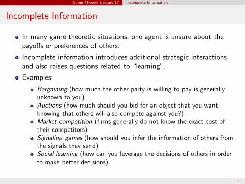
This can be established with the same graphical argument as the one we had for the complete information case.

The first graph shows the payoff for bidding one’s valuation, the second graph the payoff from bidding a lower amount, and the third the payoff from bidding higher amount.

In all cases B∗ denotes the highest bid excluding this player.

B*v*

ui(bi)

bi = v*

B*v* B*v*

bi < v* bi > v*

ui(bi) ui(bi)

bi bi

25



Moreover, now there are no other optimal strategies and thus the (Bayesian) equilibrium will be unique, since the valuation of other players are not known. Therefore, we have established:

Proposition

In the second price auction, there exists a unique Bayesian Nash equilibrium which involves

βII (v ) = v .

It is straightforward to generalize the exact same result to the situation in which bidders’ values are not independently and identically distributed. As in the complete information case, bidding truthfully remains a weakly dominant strategy. The assumption of private values is important (i.e., the valuations are known at the time of the bidding).

26



Let us next determine the expected payment by a bidder with value v , and for this, let us focus on the case in which valuations are independent and identically distributed

Fix bidder 1 and define the random variable y1 as the highest value among the remaining N − 1 bidders, i.e.,

y1 = max{v2, . . . , vN }.

Let G denote the cumulative distribution function of y1.

Clearly,G (y ) = F (y )N−1 for any y ∈ [0, v̄ ]

27



In a second price auction, the expected payment by a bidder with value v is given by

m II (v ) = Pr(v wins) × E[second highest bid | v is the highest bid] = Pr(y1 ≤ v ) × E[y1 | y1 ≤ v ] = G (v ) × E[y1 | y1 ≤ v ]. Payment II

Note that here and in what follows, we can use strict or weak inequalities given that the relevant random variables have continuous distributions. In other words, we have

Pr(y1 ≤ v ) = Pr(y1 < v ).

28


Example: Uniform Distributions

Suppose that there are two bidders with valuations, v1 and v2, distributed uniformly over [0, 1]. Then G (v1) = v1, and

E[y1 | y1 ≤ v1] = E[v2 | v2 ≤ v1] = v

2 1 .

Thus 2

II (v ) = v

m . 2

If, instead, there are N bidders with valuations distributed over [0, 1],

G (v1) = (v1)N−1

E[y1 | y1 ≤ v1] = N

N − 1

v1,

and thus II (v ) =

N − 1 N m v . N

29

�

�


First Price Auctions

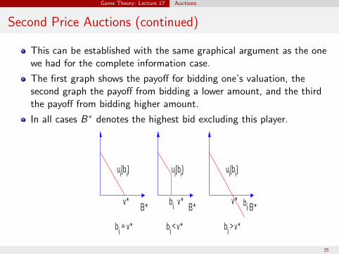
In a first price auction, each bidder submits a sealed bid of bi , and given these bids, the payoffs are given by

Ui ((bi , b−i ) , vi ) = vi − bi if bi > maxj �=i bj

0 if bi > maxj=i bj .

Tie-breaking is similar to before.

In a first price auction, the equilibrium behavior is more complicated than in a second-price auction.

Clearly, bidding truthfully is not optimal (why not?).

Trade-off between higher bids and lower bids.

So we have to work out more complicated strategies.

30

�


First Price Auctions (continued)

Approach: look for a symmetric (increasing and differentiable) equilibrium.

Suppose that bidders j = 1 follow the symmetric and differentiable equilibrium strategy βI = β, where

βi : [0, v̄ ] → R+.

We also assume that β is increasing.

We will then allow player 1 to use strategy β1 and then characterize β such that when all other players play β, β is a best response for player 1. Since player 1 was arbitrary, this will complete the characterization of equilibrium.

Suppose that bidder 1 value is v1 and he bids the amount b (i.e., β (v1) = b).

31

�

� �



First, note that a bidder with value 0 would never submit a positive bid, so

β(0) = 0.

Next, note that bidder 1 wins the auction whenevermaxi =1 β(vi ) < b.

Since β( ) is increasing, we have ·

max β(vi ) = β(max vi ) = β(y1), i=1 i=1

where recall thaty1 = max{v2, . . . , vN }.

This implies that bidder 1 wins whenever y1 < β−1(b).

32

� � �



Consequently, we can find an optimal bid of bidder 1, with valuation v1 = v , as the solution to the maximization problem

max G (β−1(b))(v − b). b≥0

The first-order (necessary) conditions imply

g (� β−1(b)) � (v − b) − G (β−1(b)) = 0, (∗)

β� β−1(b)

where g = G is the probability density function of the random variable y1. [Recall that the derivative of β−1(b) is 1/β� β−1(b) ].

This is a first-order differential equation, which we can in general solve.

33

� �

�



More explicitly, a symmetric equilibrium, we have β(v ) = b, and therefore (∗) yields

G (v )β�(v ) + g (v )β(v ) = vg (v ).

Equivalently, the first-order differential equation is

d G (v )β(v ) = vg (v ),

dv with boundary condition β(0) = 0. We can rewrite this as the following optimal bidding strategy

1 v β(v ) =

G (v ) 0 yg (y )dy = E[y1 | y1 < v ].

Note, however, that we skipped one additional step in the argument:the first-order conditions are only necessary, so one needs to showsufficiency to complete the proof that the strategyβ(v ) = E[y1 | y1 < v ] is optimal.

34



This detail notwithstanding, we have:

Proposition

In the first price auction, there exists a symmetric equilibrium given by

βI (v ) = E[y1 | y1 < v ].

35


First Price Auctions: Payments and Revenues

In general, expected payment of a bidder with value v in a first price auction is given by

m I (v ) = Pr(v wins) × β (v ) = G (v ) × E[y1 | y1 < v ]. Payment I

This can be directly compared to (Payment II), which was the payment in the second price auction (mII (v ) = G (v ) × E[y1 | y1 ≤ v ]). This establishes the somewhat surprising results that mI (v ) = mII (v ), i.e., both auction formats yield the same expected revenue to the seller.

36


First Price Auctions: Uniform Distribution

As an illustration, assume that values are uniformly distributed over [0, 1]. Then, we can verify that

βI (v ) = N − 1

v . N

Moreover, since G (v1) = (v1)N−1, we again have

m I (v ) = N − 1

v N . N

37


Revenue Equivalence

In fact, the previous result is a simple case of a more general theorem.

Consider any standard auction, in which buyers submit bids and the object is given to the bidder with the highest bid.

Suppose that values are independent and identically distributed and that all bidders are risk neutral. Then, we have the following theorem:

Theorem

Any symmetric and increasing equilibria of any standard auction (such that the expected payment of a bidder with value 0 is 0) yields the same expected revenue to the seller.

38


Sketch Proof

Consider a standard auction A and a symmetric equilibrium β of A.

Let mA(v ) denote the equilibrium expected payment in auction A by a bidder with value v .

Assume that β is such that β(0) = 0.

Consider a particular bidder, say bidder 1, and suppose that other bidders are following the equilibrium strategy β.

Consider the expected payoff of bidder 1 with value v when he bids b = β(z) instead of β(v ),

UA(z , v ) = G (z)v − m A(z).

Maximizing the preceding with respect to z yields

∂ d UA(z , v ) = g (z)v − m A(z) = 0.

∂z dz

39

�


Sketch Proof (continued)

An equilibrium will involve z = v (Why?) Hence,

d m A(y ) = g (y )y for all y ,

dy

implying that

v m A(v ) =

0 yg (y )dy = G (v ) × E[y1 | y1 < v ],

(General Payment) establishing that the expected revenue of the seller is the same independent of the particular auction format.

(General Payment), not surprisingly, has the same form as (Payment I) and (Payment II).

40

MIT OpenCourseWarehttp://ocw.mit.edu

6.254 Game Theory with Engineering Applications Spring 2010

For information about citing these materials or our Terms of Use, visit: http://ocw.mit.edu/terms.

http://ocw.mit.edu

http://ocw.mit.edu/terms

Documents

Games with incomplete information: Bayesian Nash equilibria · 6.254 : Game Theory with Engineering Applications Lecture 17: Games with Incomplete Information: Bayesian Nash Equilibria