Computing Equilibria in Static Games of IncompleteInformation Using the All-Solution Homotopy∗

Patrick Bajaria, Han Hongb, John Krainerc and Denis Nekipelovd

a Department of Economics, University of Minnesota; b Department of Economics, Stanford University; c Federal

Reserve Bank of San Francisco; d Department of Economics, UC Berkeley

This Version: March 2010

Abstract

In this paper we analyze the application of numerical continuation methods to compute equilibria

in a class of static games of incomplete information. Computation of equilibria in such games

is usually a challenging task because the sets of equilibria can have complex configurations.

The all-solution homotopy approach allows one to use a set of existing path-tracking tools to

compute asymptotic approximations to the sets of equilibria at a relatively low computational

cost. We provide some results that these tools can provide asymptotically good approximations

to sets of equilibria in games. We illustrate our findings using a simple example of an entry

game with linear payoffs. We also discuss a possible approach to estimating games with multiple

equilibria using a pre-computed set of equilibria.

JEL Classification: C14; C63

Keywords: Numerical continuation; homotopy method; static games; private information

1 Introduction

During the past decade, one of the most active areas of research in industrial organization has been

the intersection of econometrics and game theory. Starting with Bjorn and Vuong (1984), researchers

have developed empirical models of discrete games. In these models, the dependent variable has been

a discrete choice (e.g. enter or don’t enter). The payoffs are determined as in a random utility model

such as a multinomial logit. They depend on exogenous variables, parameters and random preference

shocks. However, unlike a logit, the utilities also depend on the actions of “other” agents. This has

developed into a large literature with contributions by Bresnahan and Reiss (1991a), Berry (1994),

Tamer (2003a), Seim (2006), Aguirregabiria and Mira (2002) and many others.

There are two modeling approaches in this literature. In the first approach, the error terms in the

discrete choice model are common knowledge and in the second they are private information. In the

∗We thank the editor and two referees for helpful comments.

2

former case, the models can generate a large number of possible equilibrium. Many researchers, such

as Tamer (2003a), Pakes, Porter, Ho, and Ishii (2007), Shaikh and Romano (2005) and many others

have advocated bounds estimators. This allows the researchers to work with necessary conditions

from the models and not worry about equilibrium selection. In the later case, when error terms

are private information, estimation is frequently done in two stages. For example, in static models,

Bajari, Hong, Krainer, and Nekipelov (2010) show that the estimators involve simple extensions of

static logit models.

In this paper, we propose new numerical algorithms to compute the entire set of equilibrium for

private information games. These algorithms involve the application of the all solutions homotopy.

A homotopy is a numerical method that is commonly used to solve a nonlinear system of equations.

The idea behind a homotopy is quite simple and intuitive. The researcher starts with a ”simple”

problem that is easy to solve. The researcher continuously deforms this simple problem into the

problem of interest by taking a weighted average of the two problems. Under suitable conditions,

the homotopy method is able to trace a path that leads a solution of the initial system to a solution

of final system of interest.

The applicability of homotopy methods to equilibrium computations did not remain unnoticed in

the literature. For instance, Borkovsky, Doraszelski, and Kryukov (2008) provide a user guide for

equilibrium computation in games using homotopy techniques. And Besanko et al. (2007) and

Schmedders and Judd (2005) use homotopy techniques to compute equilibria in a dynamic game.

The contribution of our paper is that we propose to use a complex-valued all-solution homotopy

that is guaranteed to provide asymptotic coverage for the equilibrium sets in games of incomplete

information. To our knowledge, such a possibility has not been considered before. For example,

Schmedders and Judd (2005) focuses on equilibria in polynomial systems. Note that Watson (1990)

also considers homotopy methods in the complex plane.

Zangwill and Garcia (1980) describe the all solutions homotopy. This method is commonly used to

find all the solutions to a polynomial system of degree n. In our paper, we adapt the all solutions

homotopy to find as many roots as possible to private information games. As we show, an equilibrium

to a private information game is a fixed point that can be represented in closed form. The system

of equations characterizes the choice probabilities generated by a logit model. In section 4.2 we

show that theoretically, if the degree of the homotopy increases to infinity without bound, all the

solutions of private information games can be found under suitable regularity conditions. However,

the validity of finding all solutions by continuously increasing the order of the homopoty is mostly

a theoretical results, since we are not able to provide an algorithmic stop rule to automate the

determination of the order of the homotopy polynomial. In practice, a course of suggested action is

to increase the degree of initial polynomial system until the method can not find any more equilibria.

One computational advantage of this approach is that it is easy to parallelize on modern computers.

We report the results from a computational exercise in which we engage in computing the equilibrium

set for a simulated set of incomplete information games. We have several surprising findings. First,

3

the number of equilibria in incomplete information games appears to decrease as the complexity

of the game (e.g., the number of players and actions) increases. This is in contrast to complete

information games, in which the number of equilibrium typically increases at an exponential rate.

See for example McKelvey, McLennan, and Turocy (2006), McKelvy and McLennan (1996), Datta

(2010) and Kalaba and Tesfatsion (1991), who use homotopy to solve finite games whose equilibria

can be represented through a system of polynomial equations. This finding is interesting for a couple

of reasons. First, estimation approaches in incomplete information games have been criticized for

assuming that the econometrician can consistently estimate agent’s beliefs. Researchers have argued

that this may not be possible if agents flip back and forth between different equilibria in the data.

Our research shows that the vast majority of our games have only one equilibrium. This suggests

that this assumption may not be a bad empirical approximation. We do caution that this is merely

an example from a numerical exercise. Since Harsanyi has shown that mixed strategy equilibria of

a complete information games are limits of sequences of incomplete information games, our finding

might not generalize beyond the specific examples that we consider. Second, our research shows

that the equilibrium set of outcomes strongly depends on the incomplete information assumption.

The choice between an incomplete information and a complete information model can make very

different predictions about behavior since they have very different equilibrium sets. In applied work,

there is no rigorous criteria for choosing between these methods. Our work shows that developing

such a criteria may be very important for ensuring the credibility of estimates and counterfactual

simulations based on these models.

The point of our paper is to show that the assumption of incomplete information generates a profound

implication in terms of the properties of the equilibrium set, such as the number of equilibrium

and the predictions of the model. Which model is right is ultimately an empirical question. The

literature needs to develop hypothesis tests which are capable of reliably distinguishing between

different models and testing each specification. This is beyond the scope of this paper. The point

here is that our computational tools show us that the incomplete information assumption can matter

a great deal in empirical research.

2 The model

In the model, there are a finite number of players, i = 1, ..., n and each player simultaneously chooses

an action ai ∈ {0, 1, . . . ,K} out of a finite set. We restrict players to have the same set of actions for

notational simplicity. However, all of our results will generalize to the case where all players have

different finite sets of actions. Let A = {0, 1, . . . ,K}n denote the vector of possible actions for all

players and let a = (a1, ..., an) denote a generic element of A. As is common in the literature, we

let a−i = (a1, ...ai−1, ai+1, ..., an) denote a vector of strategies for all players, excluding player i. We

will abstract from mixed strategies since in our model, with probability one each player will have a

unique best response.

Let si ∈ Si denote the state variable for player i. Let S = ΠiSi and let s = (s1, ..., sn) ∈ S denote

4

a vector of state variables for all n players. We will assume that s is common knowledge to all

players in the game and in our econometric analysis, we will assume that s is observable to the

econometrician. The state variable is assumed to be a real valued vector, but Si is not required to

be a finite set. Much of the previous literature assumes that the state variables in a discrete games

lie in a discrete set. While this assumption simplifies the econometric analysis of the estimator and

identification, it is a strong assumption that may not be satisfied in many applications.

For each agent, there are also K + 1 preference shocks which we label as εi(ai) which are private

information to each agent. These preference shocks are distributed i.i.d. across agents and actions.

Let εi denote the 1× (K + 1) vector of the individual εi(ai). The density of εi(ai) will be denoted

as f(εi(ai)). However, we shall sometimes simplify the notation and denote the density for εi =

(εi(0), ..., εi(K)) as f(εi).

The period utility function for player i is:

ui(a, s, εi) = πi(ai, a−i, s) + εi(ai). (2.1)

The utility function in our model is similar to a standard random utility model such as a multinomial

logit. Each player i receives a stochastic preference shock, εi(ai), for each possible action ai. In

many applications, this will be drawn from an extreme value distribution as in the logit model.

In the literature, the preference shock is alternatively interpreted as an unobserved state variable

(see Rust (1994)). Utility also depends on the vector of state variables s and actions a through

Πi(ai, a−i, s; θ). For example, in the literature, this part of utility is frequently parameterized as

a simple linear function of actions and states. Unlike a standard discrete choice model, however,

note that the actions a−i of other players in the game enter into i’s utility. A standard discrete

choice model typically assumes that agents i act in isolation in the sense that a−i is omitted from

the utility function. In many applications, this is an implausible assumption.

In this model, player i’s decision rule is a function ai = ∆i(s, εi). Note that i’s decision does not

depend on the ε−i since these shocks are private information to the other −i players in the game

and, hence, are unobservable to i. Define σi(ai|s) as:

σi(ai = k|s) =

∫1 {∆i(s, εi) = k} f(εi)dεi.

In the above expression, 1 {∆i(s, εi) = k} is the indicator function that player ı’s action is k given

the vector of state variables (s, εi). Therefore, σi(ai = k|s) is the probability that i chooses action

k conditional on the state variables s that are public information. We will define the distribution of

a given s as σ(a|s) = Πni=1σ(ai|s).

Next, define Ui(ai, s, εi; θ) as:

Ui(ai, s, εi) =∑a−i

πi(ai, a−i, s)σ−i(a−i|s) + εi(ai)

where σ−i(a−i|s) =Πj 6=iσj(aj |s).(2.2)

5

In (2.2), Ui(ai, s, εi; θ) is player i’s expected utility from choosing ai when the vector of parameters is

θ. Since i does not know the private information shocks, εj for the other players, i’s beliefs about their

actions are given by σ−i(a−i|s). The term∑a−i

πi(ai, a−i, s, θ)σ−i(a−i|s) is the expected value of

πi(ai, a−i, s; θ), marginalizing out the strategies of the other players using σ−i(a−i|s). The structure

of payoffs in (2.2) is quite similar to standard random utility models, except that the probability

distribution over other agents’ actions enter into the formula for agent i’s utility. Note that if the

error term has an atomless distribution, then player i’s optimal action is unique with probability

one. This is an extremely convenient property and eliminates the need to consider mixed strategies

as in a standard normal form game.

We also define the deterministic part of the expected payoff as

πi (ai, s) =∑a−i

πi(ai, a−i, s)σ−i(a−i|s). (2.3)

It follows immediately then that the optimal action for player i satisfies:

σi(ai|s) = Prob {εi|πi(ai, s) + εi(ai) > πi(aj , s) + εi(aj) for j 6= i.} (2.4)

A common convenient assumption regarding the distribution of εi(·) is that they are i.i.d. extreme

value distributed across actions. Our computational methodology will be tailored to this case.

However, our results generalize to the case of arbitrary shock distribution with continuous density

and unbounded support via a transformation of the cumulative distribution function.

3 The Game of Entry

For expositional clarity, consider a simple example of a discrete game. Perhaps the most commonly

studied example of a discrete game in the literature is a static entry game (see Bresnahan and Reiss

(1991a), Bresnahan and Reiss (1991b), Berry (1992), Tamer (2003b), Ciliberto and Tamer (2009),

Manuszak and Cohen (2004)). In the empirical analysis of entry games, the economist typically

has data on a cross section of markets and observes whether a particular firm i chooses to enter

a particular market. In Berry (1992) and Ciliberto and Tamer (2009), for example, the firms are

major U.S. airlines such as American, United and Northwest and the markets are large, metropolitan

airports. The state variables, si, might include the population in the metropolitan area surrounding

the airport and measures of an airline’s operating costs. Let ai = 1 denote the decision to enter a

particular market and ai = 0 denote the decision not to enter the market. In many applications,

πi(ai, a−i, s) = πi(ai, a−i, s; θ) is assumed to be a linear function of a vector of parameters, e.g.:

πi (ai, a−i, s; θ) =

s′ · β + δ∑j 6=i

1 {aj = 1} if ai = 1,

0 if ai = 0

(3.5)

6

In equation (3.5), θ = (β, δ), and the mean utility from not entering is set equal to zero.2 The term

δ measures the influence of j’s choice on i’s entry decision. If profits decrease from having another

firm enter the market then δ < 0. The parameters β measure the impact of the state variables

on πi(ai, a−i, s; θ). The other functions of the model should also be considered as functions of the

relevant parameters.

The random error terms εi(ai) are thought to capture shocks to the profitability of entry that are

private information to firm i. Suppose that the error terms are distributed extreme value. Then,

utility maximization by firm i implies that for i = 1, ..., n

σi(ai = 1|s) =

exp

s′ · β + δ∑j 6=i

σj(aj = 1|s)

1 + exp

s′ · β + δ∑j 6=i

σj(aj = 1|s)

(3.6)

In the system of equations above, applying the formula in equation (2.3) implies that πi (ai, s; θ) =

s′ · β+ δ∑j 6=i

σj(aj = 1|s). Since the error terms are distributed extreme value, equation (2.4) implies

that the choice probabilities, σi(ai = 1|s) take a form similar to a single agent multinomial logit

model. We note in passing that it can easily be shown using Brouwer’s fixed point theorem that an

equilibrium to this model exists for any finite s (see McKelvey and Palfrey (1995))).

The convenient representation of equilibrium in equation (3.6) can be exploited in econometric

analysis. Suppose that the econometrician observes t = 1, ..., T repetitions of the game and it is

assumed that in each repetition the players get new draws of private shocks. Let ai,t denote the

entry decision of firm i in repetition t and let the value of the state variables be equal to st. By

observing entry behavior in a large number of markets, the econometrician could form a consistent

estimate σi(ai = 1|s) of σi(ai = 1|s) for i = 1, ..., n. In an application, this simply boils down to

flexibly estimating the probability that a binary response, ai, is equal to one, conditional on a given

set of covariates. This could be done using any one of a number of standard techniques. Note that

this approach is only feasible observationally equivalent markets always play the same equilibrium.

Given first stage estimates of σi(ai = 1|s), we could then estimate the structural parameters of the

payoff, β and δ, by maximizing a pseudo-likelihood function using (3.6). There are two attractive

features of this strategy. The first is that it is not demanding computationally. First stage estimates

of choice probabilities could be done using a strategy as simple as a linear probability model. The

computational burden of the second stage is also light since we only need to estimate a logit model.

A second attractive feature is that it allows us to view a game as a generalization of a standard

discrete choice model. Thus, techniques from the voluminous econometric literature on discrete

choice models can be imported into the study of strategic interaction. While the example considered

2Possible normalizations are formally discussed in Bajari, Hong, Krainer, and Nekipelov (2010).

7

above is simple, it nonetheless illustrates many of the key ideas that will be essential in what follows.

We can also see a key problem with identification in the simple example above. Both the first stage

estimates σi(ai = 1|s) and the term s′ ·β depend on the vector of state variables s. This suggests that

we will suffer from a collinearity problem when trying to separately identify the effects of β and δ on

the observed choices. The standard solution to this type of problem in many settings is to impose

an exclusion restriction. Suppose, for instance, a firm specific productivity shock is included in s.

In most oligopoly models, absent technology spillovers, the productivity shocks of firms −i would

not directly enter into firm i’s profits. These shocks only enter indirectly through the endogenously

determined actions of firms −i, e.g. price, quantity or entry decisions. Therefore, if we exclude the

productivity shocks of other firms from the term s′ · β, we would no longer suffer from a collinearity

problem.

4 Computing Models with Multiple Equilibria.

In the previous sections, we have either assumed that the model has a unique equilibrium (which

can be the case, for example, for a linear probability interaction model), or that only a single

equilibrium outcome out of several possible multiple equilibria is being observed in the data set.

However, in many static game models, multiple equilibria are possible. The importance of multiple

equilibria in empirical research is emphasized by many authors, including Brock and Durlauf (2001)

and Sweeting (2008). In the rest of this manuscript we present a method for estimating parametric

models of interactions in the presence of possible multiple equilibria.

In the previous sections we have considered a model with known distribution F (εi) of the error terms

and a parametric model for the mean utility functions πi (ai, a−i, θ). At every possible parameter

value θ, given the known distribution F (εi), equations (2.3) and (2.4) defined a fixed point mapping

in the conditional choice probabilities:

σi(ai|s) = Γi

(∑−i

σa−i (a−i|s) [πi (ai, a−i, s; θ)− πi (k, a−i, s; θ)] , k = 1, . . . ,K, k 6= ai

). (4.7)

For example, under the linear mean utility specification (3.5), this system of fixed point mappings

in the choice probabilities takes the form of

σi(ai = 1|s) = Γi

s′θ + δ∑a−i

σ−i(a−i|s)

, i = 1, . . . , n. (4.8)

In previous section, we have assumed that either there is a unique solution to this system of fixed

mapping with K × n equations and K × n unknown variables

σi (ai|s) ,∀ai = 1, . . . ,K, i = 1, . . . , n,

or that only one particular fixed point of this system gets realized in the observed data. However,

this system of fixed point mapping can potentially have multiple solutions, leading to the possibility

8

of multiple equilibria. In the following of this section, we will discuss how the homotopy method

can be used to compute multiple equilibria for our model of static interactions.

4.1 The homotopy method

The homotopy theory provides a set of high level conditions for the representation of a system of

equations such that its solution set consists only of continuously differentiable paths and can be

characterized by the system of basic differential equations. Various implementation algorithms can

be developed to trace out the homotopy paths. Among the different algorithms, the homotopy con-

tinuation method (which will simply be referred to as the homotopy method in the rest of the paper)

is a well known generic algorithm for looking for a fixed point to a system of nonlinear equations.

A well-designed homotopy implementation algorithm is capable of finding multiple solutions of the

nonlinear system, and in some cases, all solutions to the system.3

Our goal is to find, for all possible parameter values and realized state variables s, the solutions for

the fixed point system (4.7): σ − Γ (σ) = 0. To simplify the notation, we suppress the fact that the

choice probabilities depend on the state σ = σ (s).

The basic idea behind the homotopy method is to take a system for which we know the solution and

“transform” this system into the system that we are interested in. Formally, a homotopy is a linear

mapping between the two topological spaces of functions of the form

H (σ, τ) = τG (σ) + (1− τ) (σ − Γ (σ)) , τ ∈ [0, 1] , (4.9)

where each of H (σ, τ) and G (σ) are vectors of functions with n×K component functions: Hi,ai (σ, τ)

and Gi,ai(σ) for i = 1, . . . , n and ai = 1, . . . ,K. H (σ, τ) is the homotopy function and τ is the

homotopy parameter. Ultimately, the objective is to solve for H (σ, 0). Varying τ from 1 to 0

“maps” the function G (·) into the function Γ(·). We start with τ = 1 and choose G (σ) to be a

system for which it is very easy to obtain the solutions to G (σ) = 0. If for each 0 ≤ τ < 1, we can

solve for the nonlinear equations, H (σ, τ) = 0, then by moving along the path in the direction of

τ = 1 to τ = 0, at the end of the path we should be able to reach a solution of the original nonlinear

equations σ − Γ (σ) = 0. This path then constructs a mapping between a solution of the initial

system G (σ) = 0 and a solution to the fixed point problem of interest, σ − Γ (σ) = 0.

In practice, algorithms for solving differential equations can be used to trace the path from τ = 1

to τ = 0. In general, the solution to H (σ, τ) = 0 forms a correspondence with finite yet multiple

number of solutions at each given parameter τ . The use of complex numbers and the assumptions

for theorem 1 in section 4.2 ensure that the sequence of correspondences along τ forms a set of paths

along each of which the solution σ (τ) is uniquely defined. This is the case that we will focus in the

3 The materials in chapters 1, 2 and 18 of Zangwill and Garcia (1981) are most closely related to the all-solution

homotopty method discussed here. Information about the homotopy method can also be found in other sources

including Watson, Billups, and Morgan (1987), Kostreva and Kinard (1991), Allgower and Georg (1980) and Watson,

Sosonkina, Melville, Morgan, and Walker (1997).

9

following. From a starting point of an initial solution of a path at τ = 1, we denote the solution

along this particular path by σ (τ): H (σ (τ) , τ) = 0. By differentiating this homotopy function with

respect to τ :

d

dτH (σ (τ) , τ) =

∂H

∂τ+∂H

∂σ· ∂σ∂τ

= 0.

This defines a system of differential equations for σ (τ) with initial condition σ (1) calculated from

the solution of the (easy) initial system G (σ (1)) = 0. In order to obtain a solution σ (0) of the

original system σ − Γ (σ) = 0, numerical algorithms of nonlinear systems of differential equations

can be used to trace the path of τ = 1 to τ = 0. A regularity condition is necessary to ensure the

path monotonicity of the system of homotopy equations. An implicit assumption in the conditions

stated below is the convention of the homotopy literature that the system has to have a smooth

parameterization.

Condition 1 (Regularity). Let ∇ (τ) denote the Jacobian of the homotopy functions with respect

to σ at the solution path σ (τ):

∇ (τ) =∂

∂σRe{H (σ, τ)}

∣∣∣∣σ=σ(τ)

,

where Re{H (σ, τ)} denotes the real component of the homotopy functions. The jacobian ∇ (τ) has

full rank for almost all τ .

This condition ensures the smoothness and differentiability of the paths. It rules out cases of

pitchfork, transcritical bifurcation, branching and infinite spiraling. The mapping between G (σ)

and σ − Γ (σ) is called a conformal one if the path that links them is free of these complications.

If a homotopy system satisfies the regularity condition, it will either reach a solution or drift off to

infinity. Intuitively, this condition prevents the the paths fromm bending back on themselves. Note

that it follows from the combination of the Path Theorem and the continuous differentiability and

regularity structure of the model that the solution set consists only of paths.

The all solution homotopy is one where the initial system G (σ) is chosen such that, if we follow the

paths originating from each of the solutions to G (σ) = 0, we will reach all solutions of the original

system σ = Γ (σ) at the end of the path. An all solution homotopy has to satisfy an additional path

finiteness condition:

Condition 2 (Path Finiteness). Define H−1 (τ) to be the set of solutions σ (τ) to the homotopy

system at τ . H−1 (τ) is bounded for all 0 ≤ τ < 1. In other words, for all τ > 0.

lim||σ||→∞

H (σ, τ) 6= 0.

This condition requires that the paths do not diverge for τ (0, 1]. The reason that the requirement

of nondivergence needs to hold at τ = 1 but not at τ = 0 is very intuitive. On the one hand, if the

10

path diverges at τ = 0, then some paths emanating from an initial solution will not converge to a

solution of the target system. This is not a problem per se as long as paths from the solution set of

the initial system lead to both all solutions of the target system and to divergence. In this case we

still find all the solutions of the target system even though some of the paths diverge. On the other

hand, divergence of the path at τ = 1 is problematic. This implies that a solution of the target

system can not be reached by a path emanating from a solution of the initial system. Therefore

we might not be able to find all the solutions of the final target system. In summary, these two

conditions in combination ensures that there is a unique path intersecting each solution of the target

system, and likewise for the initial system. In addition, each path that intersects a solution of the

target system can be traced back to a solution of the initial system.

4.2 Multiple equilibria in static discrete games

As we noted in the previous section, the issue of multiple equilibria in static interaction models

amounts to the issue of computing all the fixed points to the system of equations of choice prob-

abilities defined in equation (4.7). Note that the argument to the mapping from expected utility

to choice probabilities, Γ (·), is linear in the choice probabilities of competing agents σ−i (a−i|s).Therefore, the question of possible multiplicity of equilibria depends crucially on the functional form

of Γ, which in turn depends exclusively on the assumed joint distribution of the error terms.

Except in a very special case of linear probability model with no corner solutions, the issue of

multiple equilibria typically arises. In some models, for example if we have nonlinear interactions

of the individual choice probabilities in the linear probability model, or if the joint distribution of

the error term in the multinomial choice model is specified such that Γi is a polynomial function for

each i = 1, . . . , n, then all the equilibria can be found by choosing a homotopy system where the

initial system of equations Gi,ai (σ) for i = 1, . . . , n and ai = 1, . . . ,K. takes the following simple

polynomial form:

Gi,ai(σ) = σi (ai)qi,ai − 1 = 0 for i = 1, . . . , n and ai = 1, . . . ,K, (4.10)

where qi,ai is an integer that exceeds the degree of the polynomial of Γi,ai as a function of σ−i (a−i).

This results in a homotopy mapping

Hi,ai(σ, τ) = τ{σi (ai)qi,ai − 1}+ (1− τ) (σi (ai)− Γi,ai(σ)) , τ ∈ [0, 1]. (4.11)

For τ = 0 the system (4.9) coincides with the original system while for τ = 1 it is equal to the

’simple’ system (4.10).

It is a well known result from the foundation of complex analysis (see e.g. Zangwill and Garcia

(1981)) that there are exactly qi,ai complex roots to Gi,ai (σ) that are evenly distributed on the

unit circle. Nondegenerate polynomial functions are analytic and the regularity condition of the

resulting homotopy system is automatically satisfied. The particular choice of qi,ai also ensures the

path finiteness property of the homotopy system for 0 < τ ≤ 1 (c.f. pp355-356 of Zangwill and

Garcia (1981)).

11

While a polynomial model for Γ (·) is convenient for calculating multiple equilibria, it is rarely used

in applied problems because it is not clear what parametric utility specification will give rise to a

polynomial choice probability function. The most popular multinomial choice probability functions

are probably the multinomial logit, the ordered logit, and the multinomial probit models. Our

analysis in the following will consist of three steps. First we will establish that the incopmlete

information game model in 4.7 with possible alternative error specifications has have a finite number

of equilibria represented by real solutions. Second, we will show that by letting the degree of the

initial polynomial system increase to infinity at an appropriate rate, the homopoty method will be

able to find all the equilibria for the multinomial logit choice model (4.7). We prove it by first

verifying that the homotopy mapping is regular in the complex space when the discontinuity points

of the original function are isolated, and then providing a method to make homotopy work in the

small vicinity of discontinuity points.

To show that the fixed point system (4.7) has a finite number of solutions in the real line, note

that in general, this function is clearly continuous and infinitely differentiable with nonsingular

derivatives. Therefore Brouwer’s fixed point theorem will apply. It is easy to verify this condition

for the multinomial logit and probit models that are commonly used in practice. Consider a compact

ball BR in RnK with radius larger than 1. By Sard’s theorem the set of irregular values of Γ (σ)−σhas measure zero. It can be verified by differentiation through the implicit function theorem that

zero is its regular value. This implies that the submanifold of σ satisfying Γ (σ) − σ is a compact

subset of this ball BR, which contains a finite number of points. This verifies that the set of solutions

in BR in finite. Obviously, all the solutions must satisfy 0 ≤ σi (ai) ≤ 1. Therefore there can not be

solutions outside BR. However, the validity of finding all solutions by continuously increasing the

order of the homopoty is mostly a theoretical results, since we are not able to provide an algorithmic

stop rule to automate the determination of the order of the homotopy polynomial. In practice, we

suggest a course of action to increase qi,a until the method can not find any more equilibria.

While we have just shown that there are in general a finite number of multiple equilibria, to compute

these equilibria we need to make use of an all solution homotopy system defined in (4.11). In the

following we will show that with a sufficiently high orders of the initial system qi,ai ’s, a homotopy

system of the form of (4.11) will find all the solution to the original system of choice probabilities.

Verifying the validity of the all solution homotopy requires specifying the particular functional form

of the joint distribution of the error terms in the latent utilities and checking the regularity condition

and the path finiteness condition, which in turn require extension of the real homotopy system into

the complex space.

The following Theorem 1 and Theorem 2 formally state this result. In the statement of the theorems,

σ = {σr, σi} denotes more generally a vector of the real part and the imaginary part of complex

numbers which extend the real choice probabilities we considered early into the complex space.

Theorem 1 first establishes the regularity properties of the homotopy outside the imaginary subspace.

12

THEOREM 1. Define the sets H−1 = {(σr, σi, τ) | H(σr, σi, τ) = 0} and

H−1(τ) = {(σr, σi) | H(σ, τ) = 0} for σr ∈ RnK , and σi ∈ RnK .

Note that H is a homotopy of dimension R2nK that include both real and imaginary parts separately.

Also define, for any ε that is sufficiently small, ℘ε = ∪i,ai{|σr,i,ai | ≤ ε} to be the area around the

imaginary axis, where σr,i,ai denotes the component of the σr vector that corresponds to the ith

player’s action ai. Then:

1) The set H−1 ∩ {R2nK \ ℘ε × [0, 1]} consists of closed disjoint paths that do not intersect each

other.

2) For any τ ∈ (0, 1] there exists a bounded set such that H−1(τ) ∩ R2nK \ ℘ε is in that set.

3) For (σr, σi, τ) ∈ H−1 ∩ {R2nK \ ℘ε × [0, 1]} the homotopy system allows parametrization

H(σr(ω), σi(ω), τ(ω)) = 0.

Moreover, τ(ω) is a monotone function.

Remark: Theorem 1 establishes the regularity and path finiteness conditions for the homotopy

(4.11) in areas that are not close to the pure imaginary subspace in the complex domain CnK . The

homotopy system can become irregular along the pure imaginary subspace, because the denominator

in the system can approach zero and the system will become nonanalytic in the case. However, the

next theorem implies that if we continue to increase the power qi,ai of the initial system (4.10) of

the homotopy, we will eventually be able to find all the solutions to the original system. This also

implies, however, we might lose solutions when we continue to increase qi,ai . But Theorem 2 does

imply that for sufficiently large qi,ai , no new solutions will be added for larger powers. In the Monte

Carlo simulation that we will report in the next section, we do find this to be the case.

THEOREM 2. For given τ one can pick the power qi,ai of the initial function (4.10) such that the

homotopy system is regular and path finite given some sequence of converging polyhedra ℘ε, ε→ 0.

5 Numerical Application

We perform several numerical simulations for an entry game with a small number of potential

entrants. Player’s payoff functions for each player i were constructed as linear functions of the

indicator of the rival’s entry (ai = 1), market covariates and a random term:

ui(ai = 1, a−i) = θ1 − θ2

∑j 6=i

1(aj = 1)

+ θ3x1i + θ4x2 + εi(a), i = 1, . . . , n.

The payoff of staying out is equal to Ui(ai = 0, a−i) = εi(a), where the εi (a) have i.i.d extreme value

distributions across both a and i. The coefficients in the model are interpreted as: θ1 is the fixed

13

benefit of entry, θ2 is the loss of utility when one other player enters, θ3, θ4 are the sensitivities of

the benefit of entry to market covariates, which serve as the observed state varibles of the model.

The game can be solved to obtain ex-ante probabilities of entry in the market. The solution to this

problem is given by:

Pi =eθ1−θ2(

∑j 6=i Pj)+θ3x1i+θ4x2

1 + eθ1−θ2(∑j 6=i Pj)+θ3x1i+θ4x2

, i = 1, . . . , n.

Here Pi is the ex-ante probability of entry for the player i, Pi = p (ai = 1|x). Both coefficients of

the model and market covariates were taken from independent Monte-Carlo draws. The parameters

of generated random variables are presented in Table 1. The means and variances of parameter

values and market covariates were chosen so to have a fair percentage of cases with more then one

equilibrium. For the games with 3,4 and 5 players 400 independent parameter combinations for

every player were taken. The modification of the HOMPACK algorithm was run to solve for all

equilibria in each game.

Before we present the simulation results, we should note that the paths that follow from Theorems

1 and 2 are drawn through the complex space and do not necessarily lead to real solutions. The

existence of real solutions, however, is guaranteed by Brouwer’s fixed point theorem. In general

they can certainly lead to non-zero imaginary component. Therefore at least one of the complex

solutions has to have a zero imaginary component. In this example the number of equilibria at each

parameterization can not be determined analytically. An alternative approach is to examine a model

in which the number of equilibria can be analytically determined, e.g. Grieco (2010), even though

models with these analytic solutions may not be reflective of the types of games one typically solves

in empirical applications. We did not pursue this alternative approach.

Throughout the Monte-Carlo runs both coefficients and covariates x1 and x2 were changing. So,

every equilibrium was calculated for a specific set of parameters. Summary statistics for the results

of computations are presented in Table 2 to 4. It is possible to see from these tables that in the

constructed games the players have approximately same average entry probabilities in every type

of game. While the first two entry probabilities in Table 4 are visibly lower, they are still within

standard errors. This agrees with the symmetric form of underlying data generating process that

players are ex ante symmetric for each simulated draw of the coefficients and market covariates.

Tables 5-7 tabulate the frequencies of different number of equilibria that are being observed in the

simulations, classified according to the number of players in the market. Interestingly, a dominant

number of simulations have only a single equilibrium. In addition, the frequency of observing multiple

equilibria seems to decrease with the number of players in the market. In other words, we observe a

larger number of multiple equilibria in the three player case but only observe a handful of them in

the five player case. Complex solutions are discarded when results are reported the tables discussed

below.

Tables 8-10 tabulate the probability of entry of the first player classified by the number of equilibria

14

and the number of players in the market. In general, what we see from these tables is that there is

no clear correlation pattern between the entry probability and the numbers of equilibria and players

in the market.

6 Estimation with Pre-Computed Equilibria

Our technique for computing equilibria can be in principle directly used for construction of likelihood

functions in cases where there are multiple equilibria compatible with the data. However, given

that the provided algorithm is guaranteed to deliver all equilibria only asymptotically, it may be

computationally intensive and can slow down the likelihood maximization routine. Consider a simple

parametric example of entry game with an equlibrium selection mechanism based on the utilities of

players. Specifically, as in our example above, we use

πi (ai, a−i, s; θ) = s′i β + δ∑−i

1{aj = 1}

Suppose that σ∗i (s) denote equilibrium profiles and let S be the set of equilibria. Then the proba-

bilities of different equilibria are determined by the choice-specific payoffs from entry

p(σ∗(s)) =exp (

∑i νi π

∗i (1, s; θ))∑

σ∗′∈Sexp (

∑i νi π

∗′i (1, s; θ))

.

In other words, the probabilities of different equilibria in the equilibrium set are determined by the

weighted social welfare in the game. Then the system of probabilities of entry can be constructed as a

system of conditional moments depending on the observable state variables and containing unknown

parameters. As we noticed in Section 3, under the exclusion restriction, the entry probabilities

obtained from the first stage can be considered as additional variables. Thus we obtain the second-

stage system of conditional probabilities:

Pr (ai = 1 | s) =∑

σ∗(s)∈S

p(σ∗(s))exp

(s′iβ + δ

∑−i σ

∗j (sj)

)1 + exp

(s′iβ + δ

∑−i σ

∗j (sj)

) , for i = 1, . . . , n.

Given that this equation is valid for any s, the parameters can be estimated using the vector of

instrumental variables z constructed from s. Note that in this equation the conditional probability

of action is directly observable from the data, while functions σ∗j (·) need to be obtained from the

computation of equilibrium solution. Then using the instrument vector z we can construct a system

of unconditional moments

E

zPr (ai = 1 | s)−

∑σ∗(s)∈S

p(σ∗(s))exp

(s′iβ + δ

∑−i σ

∗j (sj)

)1 + exp

(s′iβ + δ

∑−i σ

∗j (sj)

) = 0, for i = 1, . . . , n.

This is an overidentified system of moments which can be used to estimate the parameters of interest

via the Generalized Method of Moments. Because of the need of solving for the equilibria for each

parameter value, this method is computationally intensive.

15

One possible way of reducing this computational burden is to use a set of pre-computed equilibia

for the same configuration of the game as in the data with “realistic” parameter values. More

specifically, we can suggest the following algorithm for computing equilibria approximations. First,

we simulate a sample of “realistic” parameter values and state variables. Second, we compute all

equilibria in the considered draws of state variables and parameters. Third, we recover the functions

corresponding to equilibrium choice probabilities as functions of state variables and parameters. In

fact, the composite object

f(θ, ν, s) =∑

σ∗(s)∈S

p(σ∗(s))exp

(s′iβ + δ

∑−i σ

∗j (sj)

)1 + exp

(s′iβ + δ

∑−i σ

∗j (sj)

)is a single-valued function of state variables and parameters and can be approximated using con-

ventional methods to obtain f(·). Fourth, substituting the expectation by summation over observed

sample we construct a system of empirical moments

1

T

T∑t=1

zt

(1 {ait = 1} − f (st, θ, ν)

)= 0, for i = 1, . . . , n, (6.12)

which is then used to estimate parameters θ and ν.

Alternatively, if one is willing to use a random coefficient specification for the parameters in the utility

function and the equilibrium selection mechanism, then one can use the importance sampling idea in

Ackerberg (2009) to construct a simulated likelihood (or a system of moments) using the distribution

of state variables used for constructing the sample of equilibria. Using this method in combination

with an importance sampling density, the sets of equilibria can be precomputed for the state variables

observed in the sample and for the simulated draws of the utility and equilibrium selection parameters

generated from the importance sampler. Then optimizing the likelihood function or the method of

moment objective function with respect to the hyperparameters of the random coefficient model will

only require recalculating the ratio of the density of the utility and equilibrium selection parameters

when the hyperparameters change to the importance sampling density. The sets of equilibiria do

not need to be recomputed for different evaluations of the hyperparameters.

7 Conclusion

In this paper we provided analysis of the all-solution homotopy method applied to compute all

equilibria in the static games of incomplete information. Computation of equilibria in such games

is usually a challenging task because the best-response correspondences can be highly nonlinear

and the sets of equilibria can have complex configurations. The all-solution homotopy approach

allows one to use a set of existing path-tracking tools offered in HOMPACK package. We provide

some results that these tools can provide asymptotically good approximations to sets of equilibria in

games. We illustrate our findings using a simple example of an entry game with linear payoffs. We

also discuss a possible approach to estimating games with multiple equilibria using a pre-computed

set of equilibria.

16

References

Ackerberg, D. (2009): “A new use of importance sampling to reduce computational burden in simulation

estimation,” Quantitative Marketing and Economics, 7, 343–376.

Aguirregabiria, V., and P. Mira (2002): “Swapping the Nested Fixed Point Algorithm: A Class of

Estimators for Discrete Markov Decision Models,” Econometrica, July, 1519–1543.

Allgower, E. L., and K. Georg (1980): Numerical Continuation Methods. An Introduction. Springer-

Verlag.

Bajari, P., H. Hong, J. Krainer, and D. Nekipelov (2010): “Estimating Static Models of Strategic

Interactions,” forthcoming in the Journal of Business and Economic Statistics.

Berry, S. (1992): “Estimation of a model of entry in the airline industry,” Econometrica, 60, 889–917.

(1994): “Estimating Discrete Choice Models of Product Differentiation,” RAND Journal of Eco-

nomics, 25, 242–262.

Besanko, D., U. Doraszelski, Y. Kryukov, and M. Satterthwaite (2007): “Learning-by-Doing,

Organizational Forgetting and Industry Dynamics,” .

Bjorn, P. A., and Q. Vuong (1984): “Simultaneous Equations Models for Dummy Endogenous Variables:

A Game Theoretic Formulation with an Application to Labor Force Participation,” SSWP No. 537,

Caltech.

Borkovsky, R., U. Doraszelski, and S. Kryukov (2008): “A user’s guide to solving dynamic stochastic

games using the homotopy method,” .

Bresnahan, T., and P. Reiss (1991a): “Empirical Models of Discrete Games,” Journal of Econometrics,

48, 57—81.

(1991b): “Entry and competition in concentrated markets,” Journal of Political Economy, 99,

977–1009.

Brock, W., and S. Durlauf (2001): “Discrete Choice with Social Interactions,” Review of Economic

Studies, 68, 235–260.

Ciliberto, F., and E. Tamer (2009): “Market Structure and Multiple Equilibria in Airline Markets,”

forthcoming in Econometrica.

Datta, R. (2010): “Finding all Nash equilibria of a finite game using polynomial algebra,” Economic

Theory, 42, 55–96.

Grieco, P. (2010): “Discrete Games with Flexible Information Structures: An Application to Local Grocery

Markets,” Discussion paper, Working papers.

Kalaba, R., and L. Tesfatsion (1991): “Solving nonlinear equations by adaptive homotopy continuation*

1,” Applied mathematics and computation, 41, 99–115.

17

Kostreva, M. M., and L. A. Kinard (1991): “A differential homotopy approach for solving polynomial

optimization problems and noncoorperative games,” Computers and Mathematics with Applications, 21,

135–143.

Manuszak, M., and A. Cohen (2004): “Endogenous Market Structure with Discrete Product Differentia-

tion and Multiple Equilibria: An Empirical Analysis of Competition Between Banks and Thrifts,” working

paper.

McKelvey, R., A. McLennan, and T. Turocy (2006): “Gambit: Software tools for game theory,” .

McKelvey, R., and T. Palfrey (1995): “Quantal Response Equilibria for Normal Form Games,” Games

and Economic Behavior, 10, 6–38.

McKelvy, R., and A. McLennan (1996): “The Computation of Equilibrium in Finite Games,” in The

Handbook of Computational Economics, Vol I, ed. by H. Amman, D. A. Kendrick, and J. Rust, pp. 87–142.

Elsevier.

Pakes, A., J. Porter, K. Ho, and J. Ishii (2007): “Moment Inequalities and Their Application,” working

paper, Harvard University.

Rust, J. (1994): “Structural Estimation of Markov Decision Processes,” in Handbook of Econometrics, Vol.

4, ed. by R. Engle, and D. McFadden, pp. 3082–3146. North Holland.

Schmedders, K., and K. Judd (2005): “A Computational Approach to Proving Uniqueness in Dynamic

Games,” Computing in Economics and Finance 2005.

Seim, K. (2006): “An Empirical Model of Firm Entry with Endogenous Product-Type Choices,” RAND

Journal of Economics, 37.

Shaikh, A., and J. Romano (2005): “Inference for a Class of Partially Identified Models,” Working paper.

Sweeting, A. (2008): “The Strategic Timing of Radio Commercials: An Empirical Analysis Using Multiple

Equilibria,” forthcoming in RAND Journal of Economics.

Tamer, E. (2003a): “Incomplete Simultaneous Discrete Response Model with Multiple Equilibria,” Review

of Economic Studies, 70.

(2003b): “Incomplete Simultaneous Discrete Response Model with Multiple Equilibria,” Review of

Economic Studies, 70.

Watson, L. (1990): “Globally convergent homotopy algorithms for nonlinear systems of equations,” Non-

linear Dynamics, 1, 143–191.

Watson, L. T., S. C. Billups, and A. P. Morgan (1987): “Algorithm 652 HOMPACK: A Suite of

Codes of Globally Convergent Homotopy Algorithms,” ACM Transactions on Mathematical Software, 13,

281–310.

Watson, L. T., M. Sosonkina, R. C. Melville, A. P. Morgan, and H. F. Walker (1997): “Algorithm

777: HOMPACK90: A Suite of Fortran 90 Codes for Globally Convergent Homotopy Algorithms,” ACM

Transactions on Mathematicsl Software, 23, 514–549.

18

Zangwill, W. I., and C. B. Garcia (1980): “Global Continuation Methods for Finding All Solutions to

Polynomial Systems of Equations in N Variables,” in Extremal Methods and Systems Analysis, Lecture

Notes in Economics and Mathematical Systems, ed. by A. V. Fiacco, and K. O. Kortanek, pp. 481–498.

Springr-Verlag.

(1981): Pathways to Solutions, Fixed Points, and Equilibria. Prentice-Hall.

A Proof for Theorem 1

In order to clarify manipulations and mathematical notations, in the following we will focus on the multi-

nomial logit case which is the most widely used discrete choice model in the empirical literature. Similar

results can be obtained for other multinomial choice models, including the ordered logit model.

Before we set out to prove the theorem we need to introduce some notations. Collapse the indexation for

i = 1, . . . , n and ai = 1, . . . ,K to a single index j = 1, . . . , nK. In other words, each j represents a (i, ai)

pair. First we will rewrite the expression (4.8) for the case of multinomial choice probability as:

σj =exp (Pj(σ))

1 +∑k∈Ii exp (Pk(σ))

, (A.13)

where Ii = {(i, ai) , ai = 1, . . . ,K} is the set of all indices j = (i, ai) that corresponds to the set of strategies

available to player i, and Pj (σ) is the expected utility associated with player i for playing ai when j = (i, ai):

Pj (σ) = Pi,ai (σ) =∑a−i

σ−i (a−i|s) Φi (ai, a−i, s)′ θ,

which is in general a polynomial function in σj . Let P(·) denote the vector-function of polynomials of size

nK × 1 that collects all the elements Pj(·) for j = 1, . . . , nK. Let Q be the product of the degrees of the

polynomial over all elements of the vector P(·). In other words, Q =∏nKj=1 Qj where Qj is the degree of

polynomial Pj(·). For each complex argument ξ ∈ CnK the system of polynomials has exactly Q solutions.

Because of this, for each ξ ∈ CnK we can find Q vectors σ∗ such that P(σ∗) = ξ. Let us denote each

particular vector σ∗ by P−1(k)(ξ).

The complex-valued vector P(·) of dimension nK×1 can be transformed into a real-valued vector of dimen-

sion 2nK × 1 by considering separately real and complex part of vector P(·). Because of the polynomial

property, each P−1(k) (ξ) is a continuously differentiable function of ξ for almost all ξ. It is possible that for

some range of the argument ξ, two (or more) solution paths P−1(k) (ξ) and P−1

(k′) (ξ) for k 6= k′ might coincide

with each other. In this case we will relabel the paths k so that the merged paths create a total Q of smooth

solution paths P−1(k) (ξ).

The following analysis will apply to each individual branch P−1(k) (ξ), which we will just denote by P−1 (ξ)

without explicit reference to the path indice k. For j = 1, . . . , nK introduce the following notations: ξj =

xj + iyj , ρj = ‖ξj‖, ϕj = arctan(yjxj

). Then a homotopy system can be constructed for (A.13) as:

H1j(ξ, τ) = {ρqj cos(qϕj)− 1}τ + (1− τ){Re{P−1(ξ)}−

− e2xj+e

xj cos(yj)+∑k 6=j e

xj+xk cos(yj−yk)

1+∑k∈Ii

e2xk+2∑k∈Ii

exk cos(yk)+∑l∈Ii

∑k 6=l e

xk+xl cos(yl−yk)

}

19

and

H2j(ξ, τ) = {ρqj sin(qϕj)− 1}τ + (1− τ){Im{P−1(ξ)}−

− exj sin(yj)+

∑k 6=j e

xk+xj sin(yj−yk)

1+∑k∈Ii

e2xk+2∑k∈Ii

exk cos(yk)+∑l∈Ii

∑k 6=l e

xk+xl cos(yl−yk)

}

If the system P(·) is polynomial, P−1 (ξ) is smooth and has a Jacobian of full rank for almost all ξ. Therefore,

we can locally linearize it so that P−1(ξ) ≈ Λξ + C. (This expansion is used only for the purpose of clarity.

A sufficient fact for the validity of the proof is that there exist Λ and C such that |P−1(ξ)| ≤ Λ|ξ|+ C which

is true if P(·) is a polynomial.) The homotopy system can then be written as:

H1j(ξ, τ) = {ρqj cos(qϕj)− 1}τ + (1− τ){

Λjxj−

− e2xj+e

xj cos(yj)+∑k 6=j e

xj+xk cos(yj−yk)

1+∑k∈Ii

e2xk+2∑k∈Ii

exk cos(yk)+∑l∈Ii

∑k 6=l e

xk+xl cos(yl−yk)

}(A.14)

and

H2j(ξ, τ) = {ρqj sin(qϕj)− 1}τ + (1− τ){

Λjyj−

− exj sin(yj)+

∑k 6=j e

xk+xj sin(yj−yk)

1+∑k∈Ii

e2xk+2∑k∈Ii

exk cos(yk)+∑l∈Ii

∑k 6=l e

xk+xl cos(yl−yk)

}(A.15)

where Λj is the jth row of the nK×nK matrix Λ. Without loss of generality we will let C = 0 in subsequent

analysis for the sake of brevity because all the results will hold for any other given C. To simplify notation

we will denote:

Θi(x, y) =∑k∈Ii

e2xk + 2∑k∈Ii

exk cos(yk) +∑l∈Ii

∑k 6=l

exk+xl cos(yl − yk)

Now given some index k ∈ {1, . . . , Q}, we consider the solutions of the system {H(x, y, τ)} = 0 for all

possible real values of the vectors of x and y.

Now we set out to prove the statements of Theorem 1. First we will prove statement (2). Define ρ = ‖ξ‖ to

be the Euclidean norm of the entire nK × 1 vector ξ. We need to prove that there will not be a sequence of

solutions along a path where ρ → ∞. We will show this by contradiction. Consider a path where ρ → ∞.

Choose the component j of the homotopy system for which ρqj cos(q ϕj)→∞ at the fastest rate among all

the possible indexes j where ρj →∞. 4

Consider the real part of the homotopy function, H1j(·, ·, ·). The equation H1j(x, y, τ) = 0 is equivalent to

the equationH1j(x,y,τ)

τ(ρqj cos(q ϕj)−1)= 0 for ρj > 1. The last equation can be rewritten as:

1 +(1− τ)

τ(ρqj cos(q ϕj)− 1

) {Λjx−e2xj + exj cos(yj) +

∑k 6=j e

xj+xk cos(yj − yk)

1 + Θi(x, y)

}= 0. (A.16)

4In case when instead of ρqj cos(q ϕj)→∞ we have that ρqj sin(q ϕj)→∞, the proof can be appropriately modified

by considering the imaginary part of the j-th element of the homotopy system without any further changes. The logic

of the proof can be seen to hold as long as there is a slower growing element of x or y. In case when all components of

x and y grow at the same rate to infinity in such a way that the second terms inside the curly brackets of (A.14) and

(A.15) explode to infinity, one can take a Laurent expansion around the values of yk’s such that the denominators

are close to zero. Then one can see that these terms in (A.14) and (A.15) explode to infinity at quadratic and linear

rates in 1/(y − y∗), respectively. Therefore (A.14) and (A.15) can not both be zero simultaneously for large x and y.

20

We will show that the second term in the curly bracket of the previous equation is uniformly bounded from

above in absolute terms:∣∣∣∣e2xj + exj cos(yj) +∑k 6=j e

xj+xk cos(yj − yk)

1 + Θi(x, y)

∣∣∣∣ ≤ C and for a constant C, (A.17)

where the constant C can depend on ε. Therefore the term in the curly bracket in the homotopy (A.16) will

grow at most at a linear rate |x| ≤ Cρj . On the other hand, denominator τ(ρqj cos (qϕj)− 1

)outside the

curly bracket grows at a much faster polynomial rate for large q. Hence the second term in (A.16) is close

to 0 for large q for large values of ξ, and equation (A.16) can not have a sequence of solutions that tends to

infinity.

In other words, there exists R0 > 0 such that for any ξ = (x, y) outside ℘ε with ‖ξ‖ ≥ R0 and any τ ∈ (0, 1]

we have that H1(x, y, τ) 6= 0, that is, homotopy system does not have solutions. This implies that

H−1(τ) ∩ ℘ε ⊂ BτR0= {(x, y, τ) ∈ R2nK \ ℘ε × (0, 1] ∩ ‖ξ‖ < R0}.

This proves the statement 2).

Finally, we will prove both statements 1) and 3) of Theorem 1. Again we consider the above homotopy

system on the compact set BτR0. The homotopy function is analytic in this set so Cauchy - Riehmann

theorem holds. This implies that

∂H1j

∂xk=∂H2j

∂ykand

∂H1j

∂yk= −∂H2j

∂xk, for all j, k = 1, . . . , 2nK.

This means that if the Jacobian is considered:

Ji =

(∂H1j

∂x′∂H1j

∂y′∂H1j

∂τ∂H2j

∂x′∂H2j

∂y′∂H2j

∂τ

),

then it contains at least one 2× 2 submatrix with nonnegative determinant[∂H1j

∂xk

]2+[∂H1j

∂yk

]2. Calculating

the derivatives directly due to the fact that ε < ρ < R0 this determinant is strictly positive for all (x, y, τ) ∈BτR0

. Therefore, the implicit function theorem verifies that the pair (x, y) can be locally parameterized by

τ . Moreover, this representation is locally unique and continuous. This proves the first statement. The

same arguments above, which show that the determinant is positively almost everywhere, also immediately

implies the third statement. �

Proof of equation (A.17):

We are to bound the left hand side of equation (A.17) by a given constant. First of all we can bound the

denominator from below by

‖1 + Θi(x, y)‖ ≥

∥∥∥∥∥∥1 +∑k∈Ii

e2xk

∥∥∥∥∥∥−∥∥∥∥∥∥2∑k∈Ii

exk cos(yk) +∑l∈Ii

∑k 6=l

exk+xl cos(yl − yk)

∥∥∥∥∥∥ ,as ‖a+ b‖ ≥ ‖a‖ − ‖b‖. Then we can continue to bound:

‖1 + Θi(x, y)‖ ≥ 1 +∑k∈Ii e

2xk − 2∑k∈Ii e

xk −∑l∈Ii

∑k 6=l e

xk+xl . (A.18)

21

The last expression was obtained taking into account the fact that

maxyk, k∈Ii

‖2∑k∈Ii

exk cos(yk) +∑l∈Ii

∑k 6=l

exk+xl cos(yl − yk)‖

is attained at the point cos(yk) ≡ cos(yk − yl) = 1, ∀k, l ∈ Ii.

For the same reason, we can bound the numerator from above by∥∥∥e2xj + exj cos(yj) +∑k 6=j e

xj+xk cos(yj − yk)∥∥∥ ≤ e2xj + ‖exj cos(yj)

+∑k 6=j e

xj+xk cos(yj − yk)∥∥∥ ≤ e2xj + exj +

∑k 6=j e

xj+xk .

Recall that j - th component was assumed to be the fastest growing x component as ρ → ∞. Then from

equation (A.18) for some small but positive constant ψ we can write:

‖1 + Θi(x, y)‖ ≥ 1 + ψe2xj

Collecting terms we have that:∥∥∥e2xj+exj cos(yj)+

∑k 6=j e

xj+xk cos(yj−yk)∥∥∥

‖1+Θi(x,y)‖ ≤ 1+e2xj+e

xj+∑k 6=j e

xj+xk

1+ψe2xj

.

which is clearly uniformly bounded from above by a large constant.

The same arguments can be used by looking at the imaginary part of the homotopy system when there

exists a yj that converges to infinity at the fastest rate. �

B Proof for Theorem 2

For the clarify of exposition we will present the proof in the case of two strategies for each player. In the

case with more than two strategies for each player, the expansions for the homotopy system will be more

complex and will involve more terms in the denominator. But the proof strategy is very similar, except it

involves more points around which expansions have to be taken.

In the two strategy case, we can rewrite the homotopy system (A.14) and (A.15) as

H1j(ξ, τ) = {ρqj cos(qϕj)− 1}τ + (1− τ)

{Λjxj − e

2xj+exj cos(yj)

1+e2xj+2e

xj cos(yj)

},

and

H2j(ξ, τ) = {ρqj sin(qϕj)− 1}τ + (1− τ){

Λjyj − exj sin(yj)

1+e2xi+2exj cos(yj)

}.

We need to check the presence of solutions in the small vicinity of the imaginary axis. Now consider positive

increments of xj such that xj is equal to some small value ε. If we linear the above homotopy system around

xj = 0, we can approximate them linearly by

H1j =τqεyq−1j − (1− τ)ε

2

1

1 + cos(yj)− 1 + τ

2+ λjj(1− τ)ε+

∑k 6=j

λjkxk(1− τ)

H2j =τyqj + (1− τ)∑k

λjkyk −1− τ

2

sin(yj)

1 + cos(yj)− τ

(B.19)

22

where λjj is the j, jth element of the Λ matrix.

One can see that these two functions are continuous everywhere except for the set of points {yj = π+2πk, k ∈Z} where cos (yj) = −1.

We will prove that for appropriate large values of q this system has no solutions in the vicinity of this set.

First of all note that if we take a second order expansion of 1 + cos (yj) around some y∗j = π + 2πk we can

approximate 1 + cos (yj) ≈ 12

(yj − y∗j

)2. Then we can further linearize these two equations in (B.19) to:

H1j =τqεy∗ q−1j − λjj(1− τ)ε+

∑k 6=j

λkjxk(1− τ)− 1 + τ

2− (1− τ)ε

(yj − y∗j )2

H2j =τy∗ qj + (1− τ)λjjy∗j −

∑k 6=j

λkjyk(1− τ)− τ + (1− τ)1

(yi − y∗i )

(B.20)

where we have also used sin (yj) ≈ −(yj − y∗j

).

Now we can construct a sequence of homotopies with the order q increasing to infinity at appropriate rate

such that these homotopies do not have solutions with extraneous solution of |yj | → ∞. This sequence of

q is constructed by letting q = 1 + 1/ε, as ε→ 0. Along this sequence, we will see below that the solutions

yj − y∗j to H1j and H2j will be of different orders of magnitude. Therefore there can not solutions yj − y∗jthat simultaneously satisfy both equations H1j = 0 and H2j = 0.

To see this, consider the first part H1j = 0 of (B.20). For small ε only the first term τqεy∗ q−1j = O

(y∗ 1ε

j

)and the last term (1−τ)ε

(yj−y∗j )2dominate. Therefore the solution yj − y∗j has to have the order of magnitude

O

(√1εy∗− 1

2εj

). On the other hand, for the second part H2j = 0 of (B.20). For small ε only the first term

τy∗ qj = O

(y∗ 1ε

j

)and the last term (1− τ) 1

(yi−y∗i )dominate. Therefore the solution yj −y∗j has to have the

order of magnitude O

(y∗− 1

εj

)which increases to∞ much slower than O

(√1εy∗− 1

2εj

)as ε→∞. Therefore

there can be no solution yj to both H1j and H2j simultaneously for the sequence of q chosen above. This

proves that the homotopy is path finite along that sequence of q.

The considered homotopy function is analytic outside the balls of fixed radius around the members of

countable set of points {xj = 0, yj = π + 2πk}, k ∈ Z 5. Therefore a monotone smooth parametrization is

available except for the interior of these balls because the determinant of the Jacobian is strictly positive

everywhere else.

This establishes regularity of the homotopy and concludes the proof. �

Proof of equation (B.19): We consider each term individually. First of all

ϕ = arctan (y/ε) =π

2− arctan (ε/y) ≈ π

2− ε

y.

5Moreover, it is possible to check that the homotopy system has no solutions when all arguments are purely

imaginary in case if q is an arbitrary odd number

23

Hence, as long as q is chosen so that qπ/2 is 2kπ + π2

for some k,

cos (qϕ) = cos (q arctan (y/ε)) ≈ cos(qπ

2− q ε

y

)= sin

(qε

y

)≈ qε

y.

Together with ρq ≈ yqj , this gives the first term in H1j .

Secondly, a first order expansion around ε = 0 gives

exj sin(yj)

1 + e2xi + 2exj cos(yj)≈ 1

2+

1

2ε

1

1 + cos (yj).

Therefore the H1j is proved in (B.19).

The second part of H2j follows similarly, noting that given the choice of q where sin(qϕ) = 1, and ρqj ≈ yqj ,

and the first Taylor expansion term forexj sin(yj)

1+e2xi+2exj cos(yj)

vanishes.

End of proof for equation (B.19).

C Tables

Table 1: Characteristics of the Parameters

PARAMETER MEAN VARIANCE DISTRIBUTION

θ1 2.45 1 Normal

θ2 5.0 1 Normal

θ3 1.0 1 Normal

θ4 -1.0 1 Normal

X1 1.0 0.33 Uniform

X2 1.0 0.33 Uniform

θ3X1 + θ4X2 0.0 3.32 Mixture

Table 2: Results of Monte-Carlo Simulations, n=3

Parameter Mean Std. Dev Max Min

# of equilibria 1.592 1.175 7 1

P1 0.366 0.362 0.998 0

P2 0.36 0.367 0.995 0

P3 0.363 0.348 0.993 0.003

24

Table 3: Results of Monte-Carlo Simulations, n=4

Parameter Mean Std. Dev Max Min

# of equilibria 1.292 0.777 5 1

P1 0.278 0.328 0.981 0.001

P2 0.246 0.32 0.981 0.003

P3 0.276 0.338 0.999 0.001

P4 0.28 0.338 0.987 0.002

Table 4: Results of Monte-Carlo Simulations, n=5

Parameter Mean Std. Dev Max Min

# of equilibria 1.106 0.505 5 1

P1 0.104 0.201 0.964 0

P2 0.138 0.252 0.975 0

P3 0.315 0.338 0.992 0

P4 0.356 0.385 0.983 0

P5 0.319 0.344 0.982 0

Table 5: Frequencies for the number of equilibria, n=3

# of equilibria Number of Cases Frequency (%)

m=1 192 47.93

m=3 132 33.06

m=5 64 16.12

m=7 12 2.89

Total 400 1

D Further illustrations

In this section we provide more illustrations of the two player case for the entry game example in the

the numerical application section 5. For the two player case of that example, the system of equations

characterizing the Bayes-Nash equilibrium takes the form

F1(σ1, σ2) = σ1 −exp

(θ1 + θ2σ2

)1 + exp

(θ1 + θ2σ2

) , F2(σ1, σ2) = σ2 −exp

(θ1 + θ2σ1

)1 + exp

(θ1 + θ2σ1

) ,because the structure of the model can be summarized by two parameters θ1 = θ1+θ3x1+θ4x2 and θ2 = −θ2.

To illustrate the equilibrium structure of this model, we plot the dependence of the number of equilibria

25

Table 6: Frequencies for the number of equilibria, n=4

# of equilibria Number of Cases Frequency (%)

m=1 287 71.84

m=3 93 23.3

m=5 20 4.85

Total 400 1

Table 7: Frequencies for the number of equilibria, n=5

# of equilibria Number of Cases Frequency (%)

m=1 373 93.16

m=3 25 6.21

m=5 2 0.62

Total 400 1

Table 8: Entry Probability of First Player, n=3

# of equilibria Mean STD

m=1 0.375 0.386

m=3 0.337 0.341

m=5 0.353 0.322

m=7 0.601 0.367

Table 9: Entry Probability of First Player, n=4

# of equilibria Mean STD

m=1 0.211 0.3

m=3 0.431 0.328

m=5 0.129 0.235

found using the all-solution homotopy as a function of the parameters θ1 and θ2 One can see a jump in

the number of found equilibria from 1 to 3 with the change of the parameter values. To compare the

computational results we also build a natural homotopy. For the natural homotopy we use the same system

but it is constructed for the real-valued arguments. As an initial system we use a simple system z1 = a1 and

z2 = a2. We select 100 different initial systems for each parameter pair(θ1, θ2

), and select the initial points

26

Table 10: Entry Probability of First Player, n=5

# of equilibria Mean STD

m=1 0.116 0.216

m=3 0.08 0.206

m=5 0.007 0.232

Figure 1: Number of solutions for all-solutions (a) and natural (b) homotopies

Theta 1

The

ta 2

0 1 2 3 4 5

−4.4

−4.2

−4

−3.8

−3.6

−3.4

−3.2

−3

−2.8

−2.6

n=1

n=3

Theta 1

The

ta 2

0 1 2 3 4 5 6 7 8 9 10

−4.4

−4.2

−4

−3.8

−3.6

−3.4

−3.2

−3

−2.8

−2.6

n=1

n=2

n=3

n=2

n=2

n=3

(a) (b)

uniformly over the square (σ1, σ2) ∈ [0, 1] × [0, 1]. One can see that the all-solution homotopy is capable

of finding all three solutions of the equilibrium system. The natural homotopy only finds 2 solutions for a

large combination of parameter values. This illustrates the inferior behavior of using natural homotopy for

computing the Bayes-Nash equilibria in this particular example.

We also analyzed how the behavior of the all-solution homotopy depends on the degree of the initial system.

At the parameter values θ1 = 5 and θ2 = −2.45 where the considered equilibrium system has three solutions,

We found that when q = 2, the all-solution homotopy finds 2 roots of the equilibrium system corresponding

to the stable Bayes-Nash Equilibria. However, when the degree of the initial system increases to q = 3, the

all-solution homotopy finds all three roots. This leads us to conclude that the behavior of the all-solution

homotopy for the logistic system of two equations resembles the behavior of the all-solution homotopy for

polynomials.

In the following we provide a more detailed discussion of the homotopy construction for the 2-player case.

Readers not interested in these details may skip the remaining materials. To construct the homotopy system

we first re-defined the original system of equations in the complex domain. To do that we make and additional

change of variable z1 =(σ1 − θ1

)/θ2 and z2 =

(σ2 − θ1

)/θ2. Then we set z1 and z2 to be complex such that

z1 = x1 + iy1 and z2 = x2 + iy2, where i =√−1. This produces the complex-valued system of equations

27

from the equilibrium system. We separate real and complex parts of this system creating the system with 4

unknown variables (corresponding to the real and imaginary parts of z1 and z2) that consists of 4 equations

corresponding to the real and imaginary parts of the equilibrium system. We recall the notion of hyperbolic

sine and cosine functions: sh x = 0.5(ex − e−x) and ch x = 0.5(ex + e−x) and write the real and imaginary

parts of the system of equations under consideration as:

Re (F1) =x1 − θ1

θ2− 1

2

exp (x2) + cos(y2)

ch (x2) + cos(y2),

Re (F2) =x2 − θ1

θ2− 1

2

exp (x1) + cos(y1)

ch (x1) + cos(y1).

Im (F1) =y1

θ2− 1

2

sin(y2)

ch (x2) + cos(y2),

Im (F2) =y2

θ2− 1

2

sin(y1)

ch (x1) + cos(y1).

We denote the vector-function containing the elements of this system F (x1, x2, y1, y2) and we aim at finding

all solutions of the system F (x1, x2, y1, y2) = 0. To solve this system we define an initial system of equations

G1(z1, z2) = zq1 − 1,

G2(z1, z2) = zq2 − 1.

We note that equation zq1 = 1 has q different solutions in the complex domain. In fact, given that e2πin = 1

for n = 1, 2, . . ., the solutions will take the form z1 = e2πin/q. They will be geometrically different if

1 ≤ n ≤ q, creating q different roots. We can represent the complex-valued system by the real-valued system

containing its real and imaginary parts as functions of real and imaginary arguments. As a result, we can

define the initial system as

Re (G1(z1, z2)) =(x2

1 + y21

)q/2cos

(q arctg

(x1

y1

)),

Re (G2(z1, z2)) =(x2

2 + y22

)q/2cos

(q arctg

(x2

y2

)),

Im (G1(z1, z2)) =(x2

1 + y21

)q/2sin

(q arctg

(x1

y1

)),

Im (G1(z1, z2)) =(x2

2 + y22

)q/2sin

(q arctg

(x2

y2

)).

We denote this system G(x1, x2, y1, y2). Then the homotopy system takes the form

(1− τ)G(x1, x2, y1, y2) + τ F (x1, x2, y1, y2) = 0.

We then construct the system of differential equations[(1− τ)

∂G

∂x+ τ

∂F

∂x; (1− τ)

∂G

∂y+ τ

∂F

∂y

](x

y

)= F (x, y)−G(x, y).

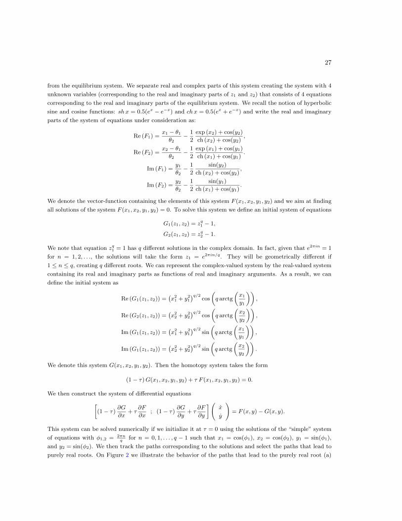
This system can be solved numerically if we initialize it at τ = 0 using the solutions of the “simple” system

of equations with φ1,2 = 2πnq

for n = 0, 1, . . . , q − 1 such that x1 = cos(φ1), x2 = cos(φ2), y1 = sin(φ1),

and y2 = sin(φ2). We then track the paths corresponding to the solutions and select the paths that lead to

purely real roots. On Figure 2 we illustrate the behavior of the paths that lead to the purely real root (a)

28

Figure 2: Homotopy path for the first dimension as a function of τ for (a) purely real solution and

(b) complex solution

0 0.1 0.2 0.3 0.4 0.5 0.6 0.7 0.8 0.9 10.49

0.5

0.51

0.52

0.53

0.54

0.55

0.56

0.57

t

X1

0 0.1 0.2 0.3 0.4 0.5 0.6 0.7 0.8 0.9 10

0.5

1

1.5

2

2.5

t

X1

(a) (b)

and a complex root (b). We display the path for the first argument of our system of interest as a function

of the homotopy parameter. An advantage of the system for 2 players is that we can explicitly solve for

the points of irregularity that correspond to the case where the matrix of first derivatives of the homotopy

system is not invertible at τ = 1. The point of irregularity correspond to the case where the denominator

in the functions of the system F (x, y) = 0 becomes equal to zero. Note that the denominator corresponding

to the first and the third equations is equal to cos (y2) + ch (x2) and the denominator of the second and

fourth equations is equal to cos (y1) + ch (x1). When (x1, x2) ∈ [0, 1]2 and (y1, y2) ∈ [−π, π]2, one of the

denominators is equal to zero if and only if x1 = y1 = 0 or x2 = y2 = 0. Thus the irregularity points will be

avoided if the homotopy path does not cross the origin.