Embed Size (px)
Citation preview

Static Games of Incomplete Information
.

Mechanism design• Typically a 3-step game of incomplete info
Step 1: Principal designs mechanism/contract
Step 2: Agents accept/reject the mechanism
Step 3: Agents that have accepted, play the game specified by mechanism
• Constant theme: Incomplete information and binding individual rationality constraints prevent efficient outcomes

Nonlinear pricing• A monopolist produces good at marginal cost c
and sells quantity q • Consumer transfers T to seller and has utility
u1(q, T, θ)= θV(q)-T, V(0)=0, V/>0, V//<0
• θ is private knowledge for buyer• Seller knows that θ= w.p. and θ= w.p. • The game:
1. Seller offers tariff T(q): specifies a price for qty q
2. Consumer accepts/rejects• If seller knows θ, she will charge T= θV(q), her
profit, θV(q)-cq. This is maximized at some q given by θV/(q)=c
p p

Nonlinear pricing• Let be bundle for type and for type• Seller’s expected profit:• Seller faces two constraints:
1. Individual Rationality (IR): Consumer should be willing to purchase
2. Incentive Compatibility (IC): Consumer should consume the bundle intended for his type
• IR1: ; and IR2:
• IC1: ; and IC2:
• First step: To show that only IR1 and IC2 are binding
) ,( Tq ) ,( Tq
)()(0 qcTpqcTpEu
0)( TqV 0)( TqV
TqVTqV )()( TqVTqV )()(

Nonlinear pricing
• First note: IR1 and IC2 imply IR2
• IR2 can’t be binding unless =0
• However, IR1 must bind. Else seller can increase
by same amount and increase revenue
• Also, IC2 must be binding, else seller can increase
, satisfy all constraints and increase revenue• The high-type’s indifference curve is always
steeper than the low type’s for any allocation• This implies that high type consumes more than
low type:
q
TT &
T

Nonlinear pricing• Eliminating transfers, principal’s objective function is:
• FOC wrt
• FOC wrt
• Check that IC1 is satisfied
• Note: Quantity purchased by high-type is optimal
Quantity purchased by low-type is sub-optimal
• Seller sacrifices efficiency for rent-extraction!
))(
1/()( : /
p
pcqVq
cqVq )( : /
)})(())()]({([max,
qcqVpqcpqVppqq
Auctions• Seller has unit of good and there are two bidders• Each bidder can have types , with < • Corresponding probabilities are and• Buyer’s expected probability of getting the good are
and payments are• The constraints are:
IR1: ; IR2:
IC1: ; IC2:
• What is seller’s optimal contract?
p p
XX & TT &
0 TX 0 TX
TXTX TXTX

Auctions • Seller’s expected profit is: • Again, IR1 and IC2 are binding. The seller’s profit:
• Also, ex-ante prob of a player getting good,• Moreover,
• Case 1: . The seller sets and Optimal mechanism: Not to sell if both announce low-type; sell to high-type if they announce different types; sell wp ½ to each if both announce high type
• Case 2: . The seller sets and Optimal mechanism: Sell to high-type if bidders announce different types, and sell wp ½ to each if they both announce high-type or low-type
TpTp
XpXpEu )(0
2
1 XpXp
2
ppX
p 0X2
ppX
p 2/pX 2
ppX

Moral Hazard
•Consider a Principal and an agent who can exert costly effort, e
•Let e {0, 1}, with costs: ψ(0)=0, ψ(1)= ψ
•Agent receives transfer, t, and has utility;
U=u(t)- ψ(e), with u/>0, u//<0.
•Production is stochastic, and production level,
,
• Stochastic influence of effort on production:
,
},{~ qqq qq
10 }1~Pr{ ;}0~Pr{ eqqeqq 01

Moral Hazard• Principal can offer a contract, {t( )}, that depends
on observed, random output• With two possible outcomes, contract is: if output
is and if output is• Let Principal’s profit with qty q be S(q)• His profit when agent expends effort e=0 is:
• His profit when agent expends effort e=1 is:
q~
q~
tq t q
])()[1(])([ 000 tqStqSV
])()[1(])([ 111 tqStqSV

Incentive Feasible Contracts
• Induce positive effort and ensure participation
• Incentive constraint:
• Participation constraint:
0)()1()( 11 tutu
)()1()()()1()( 0011 tutututu

Complete Information Benchmark• Complete info or First-Best: Principal observes effort• Principal’s problem is:
subject to:• Using Lagrangian, μ, and from FOCs we have,
• From the above equations, we have that:• Thus, Agent obtains full insurance!• The optimal transfer is: t*= u-1(ψ)=h(ψ), where h=u-1
))(1()(max 11)},{(
tStStt
0)()1()( 11 tutu
0)(
1
)(
1*/*/
tutu
*** ttt

First Best Case• When there is complete information• Principal’s profit from inducing effort e=1:
V1=
• If agent exerted 0 effort, principal would earn:
V0=
• Inducing effort is optimal for principal if: , where
• Principal’s First-Best cost of inducing effort is: h(ψ)
)()1( 11 hSS
SS )1( 00
)( hS SSS ;01

Second-Best: In terms of transfers
• Agent is risk-averse• Principal’s problem, P, is:• (P):
subject to: , and
• First ensure concavity of (P): Let
))(1()(max 11)},{(
tStStt
0)()1()( 11 tutu
)( );( tuutuu
)()1()()()1()( 0011 tutututu

Second-Best: In terms of utilities
• The Principal’s program can be rewritten in terms of utilities
• (P/):
• Principal’s objective function is concave in
because h(.) is convex, and the constraints are linear• The KKT conditions are necessary and sufficient
0)1(
)1()1( :
))()(1())((max
11
0011
11)},{(
uu
uuuutosubject
uhSuhSuu
),( uu

Both IR and IC are binding• Let λ & μ be Lagrange multipliers for IC & IR• The FOCs, upon rearranging terms, are:
where, are second-best optimal transfers
• From these, , so IR is binding
• Also, , so IC is binding
1/
1/ 1)(
1 ;
)(
1
SBSB tutu
SBSB tt ,
0)()(
1/
1/
1
SBSBtutu
0))(
1
)(
1(
)1(//
11
SBSB tutu
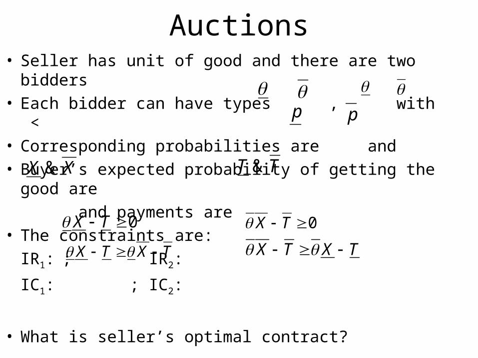
Second-Best Solution
• The variables ( , λ, μ ) are solved simultaneously from two FOCs, IC and IR
• The second-best optimal transfers are:
• : contract does not provide full insurance• 2nd Best cost of inducing effort: CSB=• Clearly, for the Principal, CSB> CFB. So Principal
induces high effort (e=1) less often than in first-best• There is under-provision of effort in the second-best
SBSB tt ,
)( );)1(( 11
htht SBSB
SBSBtt
SBSBtt )1( 11

Mechanism design with a single agent• Agent’s type with distribution/density • Type-contingent allocation is fn.• Defn: A decision function is implementable if
there exists a transfer t(.) such that allocation y(.) is incentive-compatible, i.e.
• Theorem: A piecewise C1 decision fn x(.) is implementable only if
whenever and x is differentiable at θ
] ,[ )(/)( pP
))( ),(()( txy
X:x
],[],[)ˆ,( ),),ˆ(()),(( 11 yuyu
0)/
/(
1 1
1
d
dx
tu
xu kn
k
k
)( t),( txx

Mechanism design with a single agent• Sketch of proof: Type θ announces to maximize
The FOC and SOC are
Totally differentiating the first equation,
The (local) SOC becomes or,
Rewrite the FOC we get,
Eliminating, dt/dθ,
)),ˆ(),ˆ((),ˆ( 1 txu
0ˆ
),( ,0
ˆ),(
2
2
0ˆ
),(ˆ
),( 2
2
2
01
1
1
d
dt
t
u
d
dx
x
u kn
k k
01
1
1
d
dt
t
u
d
dx
x
u kn
k k
0}/]{[ 1111
1
1
d
dx
t
u
x
u
t
u
t
u
x
u k
k
n
k k
0ˆ
),(2

Mechanism design with a single agent• The sorting/ single crossing/ constant sign (CS) condition is:
• Note that is agent’s marginal rate of substitution
between decision k and transfer t• Consider x to be output supplied by agent, i.e.,• Then sorting condition means that the agent’s indifference
curve in (x, t) space, , is decreasing in θ
• If θ2> θ1 , y(θ1)=(x(θ1), t(θ1)), y(θ2)=(x(θ2), t(θ2)), then y(θ2)>y(θ1)
• Theorem: If decision space is 1-dim and CS holds, then a necessary condition for x(.) to be implementable is that it is monotonic.
• What about sufficiency?
0/
/
1
1
tu
xu k
01 x
u
tu
xu k
/
/
1
1
tu
xu
/
/
1
1

Optimal mechanisms for one agent • The assumptions:
A1: Reservation utility independent of type
A2: Quasi-linear utilities:
Principal: u0(x, t,θ)= V0(x, θ)-t; Agent: u1(x, t,θ)= V1(x, θ)+t
A3: n=1, i.e., decision is 1-dim and CS holds.
A4:
A5:
A6:
u
012
xV
01 V
002
xV
0 & ,02
13
21
3
x
V
x
V
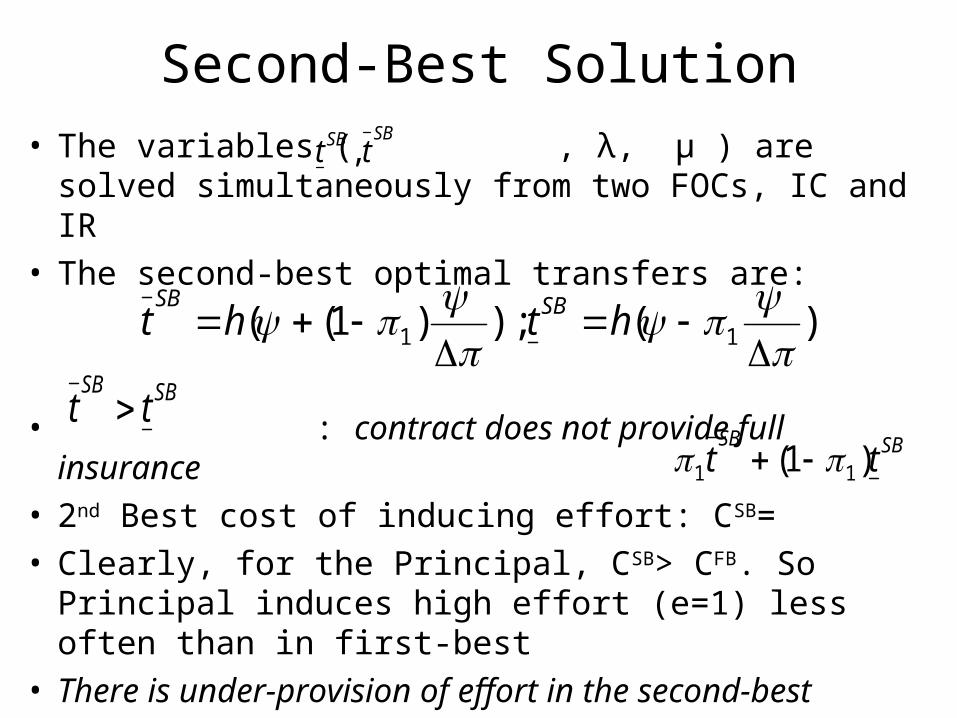
Optimal mechanisms for one agent• The problem: Principal maximizes his expected utility
subject to: (IR) u1(x(θ), t(θ), θ)≥ =0, for all θ
(IC) u1(x(θ), t(θ), θ)≥
• From A1 & A4, if IR satisfied at , it is satisfied everywhere • IR binding at . Thus, • Let
• From Envelope theorem,• This implies that,
) ),( ),((max 0)}(),({
txuE
tx
u
)ˆ ,( ) ),ˆ( ),ˆ((1 txu
0) ),( ),((1 utxu
111 Vu
d
dU
) ),( ),(() ),ˆ( ),ˆ((max)( 11ˆ1
txutxuU
~~
)~
,~
(()( 1
1 dxV
uU

Optimal mechanisms for one agent• Further, u0= V0+ V1- U1≡ Social surplus-Agent’s utility• Principal’s objective function:
• Since monotonicity is necessary and sufficient for implementability, Principal’s optimization program becomes
s.t. x(.) is monotonic
dpxV
p
PxVxV )(]
),(
)(
)(1),(),([ max 1
10{x(.)}
dpxV
p
PxVxV
dpdxV
xVxV
)(])),((
)(
)(1)),(()),(([
)(]~
~)
~),
~((
)),(()),(([
110
110
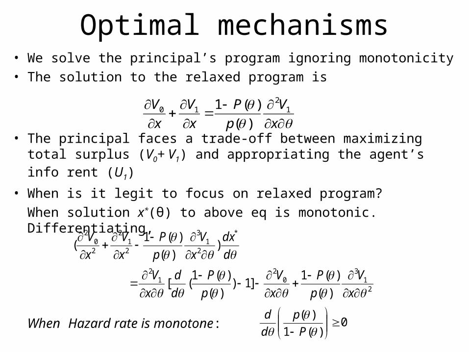
Optimal mechanisms• We solve the principal’s program ignoring monotonicity• The solution to the relaxed program is
• The principal faces a trade-off between maximizing total surplus (V0+ V1) and appropriating the agent’s info rent (U1)
• When is it legit to focus on relaxed program?
When solution x*(θ) to above eq is monotonic. Differentiating,
When Hazard rate is monotone:
x
V
p
P
x
V
x
V 12
10
)(
)(1
21
30
21
2
*
21
3
21
2
20
2
)(
)(1]1)
)(
)(1([
))(
)(1(
x
V
p
P
x
V
p
P
d
d
x
V
d
dx
x
V
p
P
x
V
x
V
0)(1
)(
P
p
d
d