Mixed Strategy Nash Equilibria in Signaling Games

Theoretical Economics Letters, 2013, 3, 52-64 http://dx.doi.org/10.4236/tel.2013.31009 Published Online February 2013 (http://www.scirp.org/journal/tel)

Mixed Strategy Nash Equilibria in Signaling Games

Barry R. Cobb1*, Atin Basuchoudhary1, Gregory Hartman2 1Department of Economics and Business, Virginia Military Institute, Lexington, USA

2Department of Mathematics and Computer Science, Virginia Military Institute, Lexington, USA Email: *[email protected], [email protected], [email protected]

Received December 3, 2012; revised January 5, 2013; accepted February 6, 2013

ABSTRACT

Signaling games are characterized by asymmetric information where the more informed player has a choice about what information to provide to its opponent. In this paper, decision trees are used to derive Nash equilibrium strategies for signaling games. We address the situation where neither player has any pure strategies at Nash equilibrium, i.e. a purely mixed strategy equilibrium. Additionally, we demonstrate that this approach can be used to determine whether certain strategies are part of a Nash equilibrium containing dominated strategies. Analyzing signaling games using a deci-sion-theoretic approach allows the analyst to avoid testing individual strategies for equilibrium conditions and ensures a perfect Bayesian solution. Keywords: Game Theory; Decision Analysis; Decision Tree; Nash Equilibrium; Signaling Game

1. Introduction

Signaling games are a class of games with incomplete information. We use the tools of decision theory to provide a process for analyzing signaling games and divide the solution process into two phases: 1) strategy selection-determining the strategies for each player that are chosen at equilibrium; and 2) equilibrium calculation-finding the percentage of each time the players should choose the selected strategies. We address this second task by solving for a purely mixed strategy Nash equilibrium. Additionally, we suggest how the approach used to solve for a purely mixed Nash equilibrium may assist in the first task, that of identifying the strategies that form an equilibrium solution.

1.1. Background

A basic signaling game has two players. Player 1 (the “Sender”) has private information about her type, while Player 2 (the “Receiver”) does not know the type of Player 1. However, Player 2 knows the population distribution of types of Player 1. Player 1 sends messages that Player 2 receives. Player 2’s actions depend on his beliefs about Player 1’s type. In a classic example of a signaling game [1], education is a signal that can be obtained by workers of both high and low skill-level. Milgrom and Roberts [2] subsequently define a limit pricing game where an incumbent firm may temporarily charge lower prices to signal that the market is unpro-

fitable. Descriptions of additional applications of signaling games have been provided by Kreps and Sobel [3] and Riley [4].

Previous research has been devoted to finding efficient Nash equilibrium solution algorithms for extensive form games. Von Stengel [5] summarizes much of the research on equilibrium calculation in extensive-form games as part of a text on algorithmic game theory [6]. While much of this research has not exclusively focused on signaling games, some of the algorithms can be used to calculate Nash equilibria in signaling games. For example, the Gambit software package developed by McKelvey et al. [7] can be used to solve signaling games. However, the developers state on the Gambit website that it is “...quite easy to write down games which will take Gambit an unacceptably long amount time to (solve).” This has been our experience in using this software to calculate Nash equilibria for signaling games. Thus, we feel there is a need to develop algorithms with heuristic approaches for determining Nash equilibria in signaling games, and this is the focus of our paper.

We suggest a method that combines modeling techni- ques from the fields of decision analysis and game theory. Previous research has combined game theory, decision analysis, and/or statistical risk analysis to address situations where the decision maker has an adaptive adversary, such as those in counterterrorism decisions. We mention some examples here. Rios Insua et al. [8] introduce a Bayesian approach to adversarial risk analysis where two or more opponents make decisions with uncertain outcomes. Decision trees and influence *Corresponding author.

Copyright © 2013 SciRes. TEL

B. R. COBB ET AL. 53

diagrams are used to simultaneously model the decision- making of each player. Parnell et al. [9] use decision tree and influence diagram models to illustrate a defender- attacker-defender problem where the United States selects actions both prior to and after a bioterrorism attack. Paté-Cornell and Guikema [10] use an influence diagram for the attacker’s decision to provide input to an influence diagram model for the defender in a counterterrorism measures selection problem.

The three articles cited above are similar to our method in that they use decision-theoretic models to examine a strategic problem from the perspective of each opponent. Our research differs in that we seek a Nash equilibrium solution (as opposed to a utility maximizing solution) and limit our analysis to problems that can be framed as a signaling game. Our primary objective is to enhance the methodology available for solving signaling games. We are optimistic that achievement of this objective will allow signaling game methodology to be applied to important decision problems that involve strategic interaction. We primarily address situations where a purely mixed Nash equilibrium exists in signaling games. Toward the end of the paper, we examine how our method can be extended to games with other types of equilibria.

Most game theory textbooks classify the equilibria for signaling games into three categories-separating on the message, pooling on the message, and semi-separating equilibria where some types of players select mixed strategies [11, pp. 326-328]. The typical analytical approach to solve for these equilibria is to assume that the equilibrium exists and then test whether either player has an incentive to deviate from the strategy or not. This process forces the game theorist to test each possible strategy pair for each of the three types of possible equilibria. In other words, the strategy selection task is by-passed and the equilibrium calculation task is sim- plified by testing only equilibria for which the mathematical conditions can be easily identified. In games with more than two types of players sending messages and/or more than two possible messages this approach can be tedious, time consuming and prone to errors.

1.2. Decision-Theoretic Approach

We suggest that a decision theoretic approach may provide a standardized process for analyzing signaling games that does not involve testing individual strategies for equilibrium qualities. Our approach can simplify both the strategy selection and equilibrium calculation tasks required to solve signaling games. This approach to solving signaling games uses the concept of Nash equilibrium. Thus, in the mixed-strategy equilibrium, each player acts in a way that makes other players indifferent between choosing among different actions.

Thus conceptually, our approach is not that different from the usual PBE (Perfect Bayesian Equilibrium) approach to solving signaling games [12]. However, the actual solution process for PBE involves testing each possible strategy for “beliefs that are consistent with strategies, which are optimal given the beliefs” [11, p. 326]. This circularity in the solution process precludes the possibility of using backward induction as a way of solving signaling games. However, in our approach we do use backward induction.

This paper uses a decision tree approach to model the two-player, n-type symmetric signaling game. The use of decision trees for representing problems of strategic interaction was introduced by van Binsbergen and Marx [13]. In their model, a decision tree is constructed for each player. A player’s own choices are modeled with decision nodes and the opponent’s strategies are shown as chance variables.

Cobb and Basuchoudhary [14] modified the decision tree approach by modeling the choices of both players in each tree with chance nodes and using the probabilities in the trees to represent the strategies. This allowed use of the decision tree approach to solve the two-type signaling game; however, this prior research only discussed the determination of pooling, separating, and semi-separating equilibria. This paper extends the previous research by both addressing signaling games with more than two types of Senders and by finding a purely mixed Nash equilibrium (the equilibrium calculation task), which is one where neither player has any pure strategies.

We employ a decision tree representation of the signaling game to determine Nash equilibrium strategies for several reasons. First, the equations capturing the Nash equilibrium strategies are actually calculated while solving the decision tree, as opposed to being abstractly determined by analyzing the game tree. This is par- ticularly advantageous in the signaling game because Bayes’ rule is used routinely at the time the decision tree is constructed. Second, the Nash equilibrium conditions are intuitively apparent through inspection of the decision tree. Additionally, the decision tree representation is more easily expanded as the number of Sender types increases than a corresponding game tree representation.

1.3. Outline

After first introducing signaling games and notation used in the paper, we solve for Nash equilibrium strategies in a two-type signaling game. The purpose of this section is to illustrate how decision trees are constructed for signaling games. Next, we give general derivations of Nash equilibrium strategies in the n-type signaling game where both players select purely mixed strategies at Nash equilibrium. In general, for a strategy vector



chosen by the Sender to be part of a purely mixed Nash equilibrium, the Receiver observing each possible message must be indifferent between all of its subsequent actions after assigning any dominated strategies for the Sender a value of zero. Similarly, for a strategy vector chosen by the Receiver to be part of a purely mixed Nash equilibrium, each type of Sender must be indifferent between transmitting each of its possible messages after assigning any dominated strategies for the Receiver a value of zero.

Later in the paper, we will discuss how to apply decision trees to signaling games where the players do not necessarily select purely mixed strategies at Nash equilibrium, i.e. we use decision trees to address the strategy selection task. In the final section, we discuss our results and describe the development of a com- prehensive approach to determining all types of equilibria in signaling games as a direction for future research.

2. Preliminaries

This section outlines notation and definitions that will be used throughout the paper.

In the n -type signaling game, the Sender has n possible types, 1 and can choose one of n possible messages, 1 , from a discrete strategy set. The Receiver responds with one of n possible actions, 1 , that it chooses from its discrete strategy set once it observes the Sender’s message. Descriptions and definitions of the parameters in the

-type signaling game are shown below.

, , nt m

na

t, , nm

, ,a

n

Parameter Description

ip Probability the sender is type i

( for )

Let us summarize the strategies played by the Sender and the Receiver, respectively, in vector form as

T11 21 1 12n nm m m m mm n

n

and

T11 12 1 21 .n na a a a aa

Note that is indexed differently than a . The first part of the index on refers to the Sender type and the second part refers to the message transmitted by the Sender. The first number in the index on

m

ijm

jka refers to the message of the Sender, whereas the second stands for the action of the Receiver. This ordering is consistent with the order in which the nodes appear in the decision trees presented throughout the remainder of the paper.

The strategy for the Sender can be interpreted as the conditional probability

ijm | j iP m t that the

Sender will transmit message it

jm . Analogously, the strategy jka for the Receiver can be interpreted as the conditional probability |k jP a m .

We use a decision tree approach to identify Nash equilibrium strategies in signaling games. We first consider the case where neither player has any dominated strategies at Nash equilibrium and address the equilibrium calculation task. In this situation, the payoffs are structured so that there is an equilibrium where each type of Sender plays a mixture of all of its possible messages, so each Sender strategy satisfies 0 1 at Nash equilibrium. Correspondingly, the payoffs are also structured so that the Receiver plays a mixture of all its possible strategies after observing each message, which requires each Receiver strategy to satisfy 0 1 .

ijm

a jk

By inspecting the decision tree models, we are able to intuitively observe the conditions that must exist for a solution to be a Nash equilibrium. The decision tree provides for easy calculation of the expected values for each player, which are ultimately used to derive the mathematical conditions necessary for a Nash equilibrium in purely mixed strategies.

it 1, ,i n

ijm it Sender’s strategy

(% of time i , , plays

message for

t n1, ,i

j 1,m ,j n )

jka Receiver’s strategy after observing message

, jm 1, ,j n

(% of time receiver takes action

for ) ka

1, ,k n

ijkv Payoff to the Receiver observing

message and taking action jm ka

when the Sender is it

ijkw Payoff to the Sender playing

message

it

jm

when the Receiver takes action ka

3. Signaling Game Example

This section analyzes a two-type signaling game. For now, we assume nature’s selection of each Sender type is equally likely, i.e. 1 2 0.5p p . The Sender will choose one of two messages-Left or Right. The selection of the Left strategy by the 1t Sender is the strategy , whereas the choice of Left for the 2t Sender is 21m . The alternate strategies (Right) are denoted by 12m and

22m for 1t and 2t , respectively, and these probabilities satisfy m

11m

12 111m and 11m m . 22 2

Once the Receiver observes the signal, it decides whether or not to move Up or Down and this threat represents its strategy. If it observes the Left message, its


B. R. COBB ET AL.


55

r and Receiver are shown in T

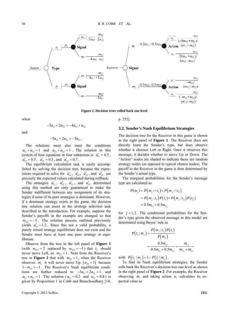
Up strategy is denoted by 11a . If it observes Right, its To find its Nash equilibrium strategies, the Receiver rolls back the Sender’s decision tree one level as shown in the left panel of Figure 2. Since all nodes in the tree are chance nodes, the roll-back procedure involves calculating expected values. For example, the 1 Sender observing 1 calculates its expected value as

11 12

tm

2 a3 a

t

at the chance node representing the Receiver action at the top of its tree in Figure 1. This expected value is placed in the rolled back decision tree in Figure 2 as the payoff on the branch representing the

1 Sender and the 1 observation. Other expected values are calculated similarly during the roll-back process.

m

Up strategy is denoted by . A Down strategy by the Receiver is denoted by eithe 12a or 22a , depending on the type of signal observed.

The payoffs for the Sende

21ar

able 1. As an example, if the Receiver moves Up against a 1t Sender, both players could suffer significant losses, thus 111 8v and 111 3w . The Sender ends u a worse in this scenario by selecting Right, so 121 4w .

p with e

3.1. Receiver’s Nash Equilibrium Strategies

n in

outcom

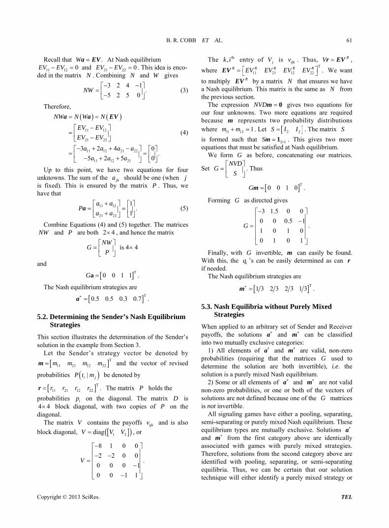
The decision tree for the Sender in this game is showTwo conditions must be met by the strategies 11 ,

12 , 21 , and established at Nash equilibrium by the Receiver:

aa a 22a

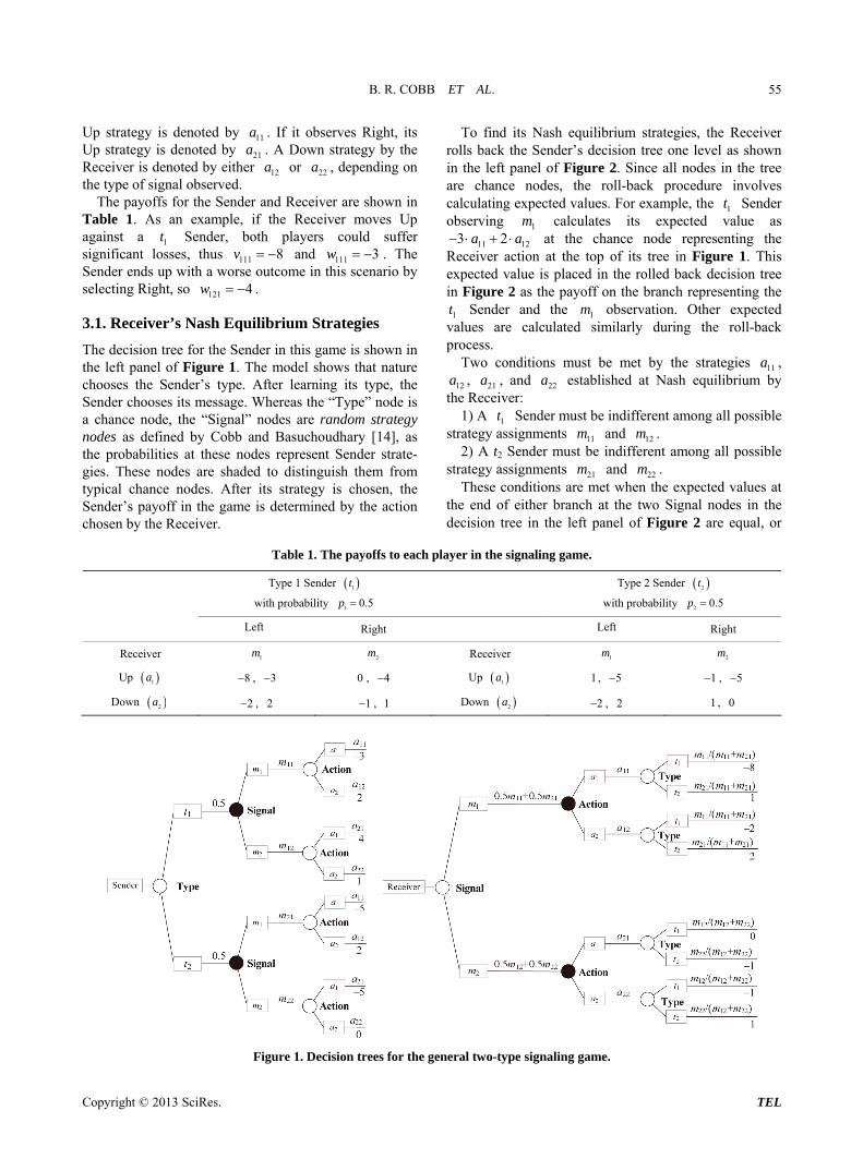
the left panel of Figure 1. The model shows that nature chooses the Sender’s type. After learning its type, the Sender chooses its message. Whereas the “Type” node is a chance node, the “Signal” nodes are random strategy nodes as defined by Cobb and Basuchoudhary [14], as the probabilities at these nodes represent Sender strategies. These nodes are shaded to distinguish them from typical chance nodes. After its strategy is chosen, the Sender’s payoff in the game is determined by the action chosen by the Receiver.

1) A 1 Sender must be indifferent among all possible strategy assignments and 2 .

t

11 1

2) A t2 Sender must be indifferent among all possible strategy assignments and 22 .

m m

21

These conditions are met when the expected values at the end of either branch at the two Signal nodes in the decision tree in the left panel of Figure 2 are equal, or

m m

Table 1. The payoffs to each player in the signaling game.

T

wi

Type 2 Sender

wi

ype 1 Sender 1t

th probability 1 0.5p

2t

th probability p2 0.5

Right L Right Left eft

Receiver Receiver 1m 2m 1m 2m

Up 1a 8 , 3 0 , 4 Up 1a 1 , 5 1 , 5

Down 2a 2 , 2 1 , 1 Down 2a 2 , 2 1 , 0

Figure 1. Decision trees for the general two-type signaling game.


Figure 2. Decision trees rolled back one level.

hen

and

.

meet the conditions

task is - lis

w

11 12 21 223 2 4a a a a

11 12 215 2 5a a a

The solutions m

1asystem of fo

The

ust also

tions in four

ation

1 12 1a and 21 22 1a a . The solution to this ur equa unknowns is 11 0.5a ,

12 0.5a , 21 0.3a , and 22 0.7a . equilibrium calcul easily accomp

hed by solving the decision tree, because the expre- ssions required to solve for 11a , 12a , 21a , and 22a are precisely the expected values cu d ring ro ck.

The strategies 11a , 12a , 21a , and 22a determined cal late du llba

us u t

e from the tree in the left panel of Figure 1 (w

ing this method are only aranteed o make the Sender indifferent between any assignment of its strategies if none of its pure strategies is dominant. However, if a dominant strategy exists in the game, the decision tree solution can assist in the strategy selection task described in the introduction. For example, suppose the Sender’s payoffs in the example are changed so that

212 5w . The solution process outlined previously 1.2 . Since this not a valid probability, a

purely mixed strategy equilibrium does not exist and the Sender must have at least one pure strategy at equilibrium.

Observ

g

yields 11a

ith 212 2w replaced by 212 5w ) that 2t should never ft, so 22 1m . Note the Receiver’s tree in Figure 2 that 22 1m , when the Receiver observes 2m it will never m p 22 1a because

121 1m The Receiver’s Nash equilibrium condi- further reduced to 11 123 2 1a a and

11 12 1a a . The solution ( 11 0.a

move Le

. re

from

ove U

2 and

with

tions a

12a 0.8 ) is position 1 in Cob asucho [14,

3.2. Sen

given by Pro b and B udhary

p. 252].

der’s Nash Equilibrium Strategies

shown es not

The decision tree for the Receiver in this game isin the right panel of Figure 1. The Receiver dodirectly learn the Sender’s type, but does observe whether it chooses Left or Right. Once it observes this message, it decides whether to move Up or Down. The “Action” nodes are shaded to indicate these are random strategy nodes (as opposed to typical chance nodes). The payoff to the Receiver in the game is then determined by the Sender’s actual type.

The marginal probabilities for the Sender’s message type are calculated as

( )j jP m P m t P m t

1 2

1 1 2 2

1 2

| |

0.5 0.5

j

j j

j j

P m t P t P m t P t

m m

1, 2j for . The conditional probabilities for the Sen- der given the observed message in this model are

rmined’s type

dete using Bayes’ rule as

1

1

||

j

j

1

1 1

1 2 1 2

0.5

0.5 0.5

j

j j

j j j j

P m

m m

m m m m

with

P m t P tP t m

2 1| 1 |j jP t m P t m . To find its Nash equilibrium strategies, the Sender

ack the Receiver’s decision tree one level as shown rolls bin the right panel of Figure 2. For example, the Receiver observing 1m and taking action 1a calculates its expected value as



11 11 21 21 11 21

11

8

8

m m m m m m

m m m m

21 11 21

at the chance node representing the Sender type at the top of its tree in Figure 1. This expected value is placed in the rolled back decision tree in Figure 2 as the pay ff on

ntbe

f

meet the conditions and . Solv system of s in gives

othe branch representing the Receiver observing 1m and taking action 1a .

Two conditions must be met by the strategies 11m ,

12m , 21m , and 22m established at Nash equilibrium by the Sender:

1) If the Re vecei r observes 1m , it must be indiffere tween the strategies 11a and 12a . 2) If the Receiver observes 2m , it must be indifferent

between the strategies 21a and 22 . These conditions are met when the expected values at

the end of either branc

a

h at the two Action nodes in the decision tree in the right panel o Figure 2 are equal, or when

11 21 11 218 2m m m m

and

22 12 22 .m m m

The solutions m

12 1m four equation

ust also

21 22 1m m four unknowns

11m ing this 11 1 3m ,

12 2 3 , m 21 2 3m , and 22 1 3m . The strategies , , 1m , and 22m determined

using the process outlined above are only guaranteed to 11m 12m 2

make the Receiver indifferent between any assignment of its strategies if none of its strategies are dominant. Recall the example from the last section where the Sender’s payoffs are such that it always plays 21 0m and

22 1m . The revised probabilities in th ver’s tree will indicate that 2 1| 0P t m . We also

established that in this scenario observing

2m should always play 21 0a and 22 1a

e Recei

iver decision

the Rece . By

ting the pure strategies th always ed by both the Sender and Receiver in the decision trees and rolling back the trees, the Nash equilibrium strategies for a semi-separating equilibrium can be determined. The solution for the Receiver observing 1m is given by Proposition 2 in Cobb and Basuchoudhar 14, p. 252].

In this next section, decision trees and the expecte

inser

va

at will

y

ral n

be play

[

-type sign

d

4. General Signaling Game

aling

lues obtained from the solution process are used to obtain a pure mixed strategy Nash equilibrium for the n -type signaling game.

In this section, we discuss the genegame. Decision trees similar to those used in the 2n case will be useful in demonstrating the conditions are required to establish a Nash equilibrium.

that

4.1. Analysis of Sender’s

r the

Decision Tree

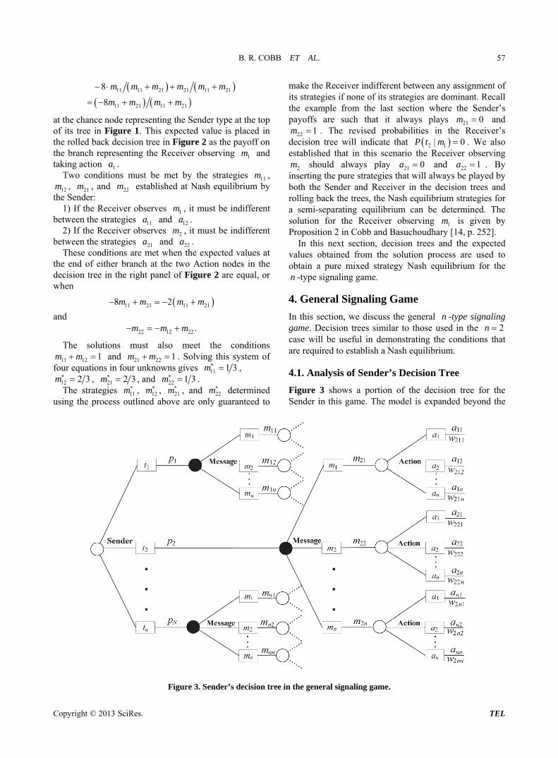
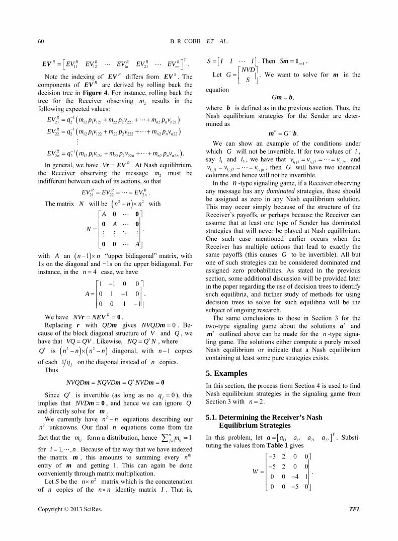
Figure 3 shows a portion of the decision tree foSender in this game. The model is expanded beyond the

Figure 3. Sender’s decision tree in the general signaling game.



“Message” branch for the Sender. This expansion shows that the Send hooses from among possible messages. Once it selects a message, it which of the ossible actions has beetaken. An expansion of the decision tree for the other Sender types would appear similarly.

Rolling back the section of the decision tree in Figure 3 for the Sender results in the expected values

2ter c

p

2t

Receiver’s

n will

n n

2t

2 1 2 1 2 2 2 2Sj j j j j jn jnEV a w a w a w

for . A Nash equilibrium in this game must m separate conditions

(1)

More generally, the Receiver’s strategies at Nash equilibrium must obey the conditions

(2)

for . s

1, ,j n eet the 1n

21 22

22 23 2, 1 2

0,

0, , 0.

S S

S S S Sn n

EV EV

EV EV EV EV

1 2

2 3 , 1

0,

0, , 0

S Si i

S S S Si i i n in

EV EV

EV EV EV EV

1, 2, ,i n To solve for the mixed trategy Nash equilibrium

strategies for the Receiver, we construct the 2 2n n matrix W as

1

2

W

WW

0

0 0,

0

nW

0 0

where each jW a

is itself an matrix and is the trix. The of block

n nkth en

0n n zero m i , try jW is simp he vector Sly ijkw . T EV is 2 1n , with

S S ST

11 21 1 12 .S S SnEV EV EV EV EVEV nn

Note that conditions specified in (1) and (2)

in

SW a EV . We can encode the the 2 2n n n matrix

I I

.I I

N

I I

0

0 0

0 0 0

0

where I is the n n identity matrix. To satisfy a Nash equilibrium, we need NWa = N 0EV This gives us 2n n equations f r

2n unk s.

nownof the

or that the sum

1 1 1

1 1 1

1 1 1

.

n n n

n n n

n n n

P

1 0 0

0 1 0

0 0 1

Thus, we want P a 1 . Let and define NW

GP

2 1

1

n n

n

b0

1. We solve in the equation

Thus, the Nash equilibrium strategies for the Receiver are determined as

provided these entries are all non-negative. When the Receiver plays the strategies in , the Sender cannot unilaterally change its strategy to earn a higher expected payoff.

The prior discussion describes how the decision tree uilibrium calculation in the

case of a purely mixed strategy equilibrium. To aid in strategy selection, the vector can be examined to determine whether there are any dominated strategies at equilibrium. This is indicated when contains entries that are not strictly between 0 not invertible. In the -type signa e, if a r of

anassig n

s i pris gies in a Nash equilibrium. Since the Receiver can assume that the Sender will never play dominated strategies, it can a ccordingly and may find do

ti strategies f iver. A well-defined algo-

rithm for finding Nash equilibria where each player chooses some pure strategies and mixes over the remaining strategies is beyond the scope of paper and requires future research. An example of such a solution in the context of a specific example will be provided later

4.2

Thg This sh eyond the “A tion”

node when the Receiver observes message . The detail shows that the Receiver will first learn the m ssage selected from the Sender’s possible choice ce it

want to for a

.G a b

1G a b

a

formulation is used for eq

a

ling

aand 1, or when

gamG is

Sende

istrate

nany type has y dominated strategies, these should be

ned zero probabilities prior to finding the rema ing strategie n a that com e the Receiver’s

djust its strategies aminated strategies of its own. The decision tree metho-

dology can s ll be useful in determining Nash equilibrium or the Rece

this

in this section.

. Analysis of Receiver’s Decision Tree

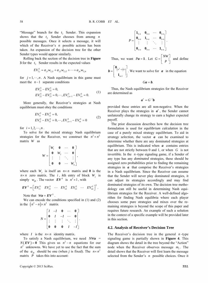
e Receiver’s decision tree in the general n -type signalin game is partially shown in Figure 4.

ouWe have yet to e fact use th

jka sh

diagram ows the detail in the tree b c

2

en

m

s. On ould be one (wh is fixed). Ten j he 2n n

takes this into account: matrix P



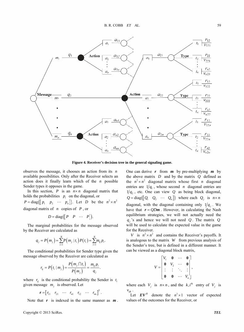
in the general signaling game. Figure 4. Receiver’s decision tree observes the message, it chooses an action from its n

available possibilities. Only after the Receiver selects an action does it finally learn which of th possiSender types it opposes in the game.

In this section, an

e n ble

P is n n the diag

diagonal matrix that holds the probabilities on onal, or ip

1 2diag .nP p p p Let be the D 2 2n n

diagonal matrix of n copies of P , or

diag .D P P P

The marginal probabilities for the message observed by the Receiver are calculated as

1 1

| .N N

j j j i ii i

q P m P m t P t m p

ij i

The conditional probabilities for Sender type given the message observed by the Receiver are calculated as

| .j i ij i

ij i jjj

P m t m pr P t m

qP m

where probability the Sender is given m ssage

ijre

is the conditional it

jm is observed. Let

Note that is indexed in the same manner .

One can derive from by pre-multiplyin by the a a an the matrix de d as the

T11 21 .n nr r r r rr 1 12 n

r as m

rtrix

md by

g mfinebove m

2 2n nD Q

al m trix whos diagon a e first n diagonalentries are 11 q , whose tries are second n diagonal en

21 q , etc. One ca onal, n view Q as being block diag

1 2diag nQ Q Q Q is n n where each jQ

al containing onldiagonal, with the diagon y 1 jq . We QDr m

strategies, we have that . However, in calequilibrium will not act

culating the Nash ually need the

jq ’s and hence we will not need . The mwill be used to calculate the expected value in the game for the Receiver.

is

Q atrix Q

V 2 2n n is analogous to the m

and contains the Receiver’s payoffs. It atrix from previous analysis of

the Sender’s tree, but is defined in a different manner. It can be viewed as a diagonal block matrix,

W

1

2 ,

n

V

VV

V

0 0

0 0

0 0

where each n njV is , and the entry of th,k i jV is

ijkv . Let REV denote the 2n

for the Receiver, 1 vector of expected

values of the outcomes or



T

11 12 1 21 .R R R R R Rn nEV EV EV EV EV EV n

Note the indexing of

REV differs from SEV . The components of REV are derived by rolling back the decision tree in Figure 4. For instance, rolling back the tre rvinge for the Receiver obse 2m results in the following expected values:

121 2 12 1 121 22 1

11 2 22

12 2 12 1 12 22 2 22 2 2 .

R

n n n

Rn n n n

EV q m p v m p

m p v

EV q m p v m p v p v

n n n

22 2 12 122 22 2 222

REV q m p v m p v 2 221 2 2n n nv m p v

m

In general, we have RV r EV . At Nash equilibrium, the Receiver observing the message must be indifferent between each of its actions, so that

2m

21 22 2R R

nEV EV EV R .

The matrix N will be 2 2n n n with

A

.A

N

A

0 0

0 0

0 0

with A an 1n n “upper bidiagonal” matrix, wit 1s on the diago and −1s on the upper

hbidiagonal. For

h case, we have

R

nal e 4n instance, in t

1 1 0 0 0 1 1 0 .

0 1 1

A

We have RN r EV 0 . eplacing r with QDm gives 0NVQD

0

NVm . Be-

of t , we cause h ock dia tructurhave that

c

e blVQ

gonal s. Likewis

e of V and QQV e, NQ Q N , where

Q is 2 2n n n n diagonal, with n opies

of each

1

1 jq on the diagonal instead of n copies. Thus

NVQD NQVD Q NVD m m m 0

Since Q is invertible (as long as no 0jq ), this implies that NVD m 0 , and hence we can ignore Q and directly solve for m .

We currently have 2n n equations describing our 2n unknowns. Our final n equations come from the

11

n

ijjm

fact that the form a distribution, hence ijm

fo . Because of the way that e have indexed this amounts to summing every

en and getting 1. This can again beatrix m

matrix which is the identity matrix

r 1, ,i n the matrix m

try of m

w, thn

done conveniently through m ultiplication.

Let S be the 2n n concatenation of copies n of the n n I

S I I I . Then 1nS m 1 .

Let NVD

GS

. We want to solve for m in the

equation

We can show an example of the conditions under which will not be invertible. If for two values of say , we have that

,G m b

where b is defined as in the previous section. Thus, the Nash equilibrium strategies for the Sender are determined as

1 .G m b

G and

2 21 2i j

i , and 1i

v v2i 1 1 11 2i j i j i jnv v v

2i j i jnv colum hence

, thenwill not

In the -type signaling game, if a Receiver observing an ominated

re of the Receiver’s payoffs, or perhaps because t Receiver can assum pe of Sende ominated strategies that will never be played at Nash equilibrium. One su case mentioned earlier occurs when the Receiver has multiple actions that lead to exactly the same (this cause to be invertible). All but one of suc strategies ca considered dominated and assigned zero probabilities. As stated in the previous

ditional di

furt ods for using decision trees to solve for such equilibria will be the subject of ongoing research.

The same conclusions to those in Section 3 for the type signaling game about the solutions

G will have two identical be invertible. ns and

n

ch

payoffs h

y message has any d strategies, these should be assigned as zero in any Nash equilibrium solution. This may occur simply because of the structu

he e that at least one ty r has d

s Gn be

section, some ad scussion will be provided later in the paper regarding the use of decision trees to identify such equilibria, and her study of meth

two- a and m outlined above can be made for the -ty -

lin he solutions either compute a purely mixed N i ndicat Nash equili

5. Examples

ind

Section 3 with

n pe signag game. T

ash equilibr um or i e that a brium containing at least some pure strategies exists.

In this section, the process from Section 4 is used to fNash equilibri strategies in the signaling game from um

2n .

5. rm

. Substi- tu

1. Dete ining the Receiver’s Nash Equilibrium Strategies

In this problem, let a aT

11 a aaable 1

12 21 22

ting the values from T gives

3 0 0 2

5 2 0 0.

0 0 4 1

0 0 5 0

W

. That is,



Recall th .W a EV At Nash equilibrium

11 12 0EV EV and 21 22 0EV EV . This iat

dea is encode Comb

efore,

(4)

Up to this point, we have two equations for four un

d in the matrix N . ining N and W gives

3 2 4 1.

5 2 5NW

(3)

0Ther

11 12

11 12 215 2 5 0

NW N W N

EV EV

EV EV

a a a

a a EV

21 22

11 12 21 223 2 4 0.

a a a a

knowns. The sum of the jka should be one (when j is fixed This is ensured by the matrix P . Thus, we have hat

11 12 1.

a aP

). t

21 22 1a a Combine Equations (4) and (5) together. The matrices

NW and P are both 2 4 , and hence the matrix

is 4 4NW

GP

and

T0 0 1 1 .G a

The Nash equilibrium stra gies are

T0.5 0.5 0.3 0.7 . a

5.2. Determining the Sender’s Nash Equilibrium Strategies

This section illustrates the determination of the Sender’s so

(5)

te

the

e diagonal. T atrix is onal, with two copies of the

a

lution in the example from Section 3. Let the Sender’s strategy vector be denoted by

T11 21 12 22m m m m and the vector of revised

probabilities |i jP t m be denoted by

T11 21 12 22 .r r r rr The matrix P holds

m

probabilities ip4 4 block dia

on th he m D on g P

diagonal. The matrix V contains the payoffs ijkv and is also

block diagonal, 1 2agV V di V , or

The

8 1 0 0

2 2 0

0

.0 0 0 1

0 0 1 1

V

th,k i entry of jV is . Thus,ijkv RV r EVT

,

where 11 21 12 22 .R R R R REV EV EV EV EV We want

to multiply REVilibrium

by a matrix that ensures we have ash equ . This matrix e same as om

th ctiThe expressi

N is tha N N fr

e previous se on. Don NV m 0

s. esents tw

givesqua re

because lity where

two equations for our four unknown Two more e tions a required

m repr

1 2 1i im mo probabi distributions

. Let 2 2S I I he matrix S . T

is that formed such 2 1S 1me satisfied at

. This gives two more eq ust b Nash equilibrium.

We form as before, concatenating our matrices.

Set

uations that m G

NVDG

S

. Thus

T0 0 1 0 .G m

Forming G as directed gives

3 1.5 0 0

0 0 0.5 1.G

1 0 1 0

0 1 0 1

Finally, with invertible, an easily be found. Wif nee

The Nash equilibrium strategies are

G m cith this, the iq ’s can be easily determined as can r

ded.

T1 3 2 3 2 3 1 3 . m

5.3. Nash Equilibria without Purely Mixed Strategies

Whe r and Receiver payoffs, the solutions

n applied to an arbitrary set of Sendea and can be classified

into two mutually exclusive categories:

m

1) All elements of a and m are valid, non-zero probabilities (requiring that the matrices G used to

ine the so

determ lution are both invertible), i.e. the

are not valid nosolutions are not defined becis not invertible.

g games ng, separating, semi-separating or purely mixed Nash equilibrium. Thequilibrium types are m ive

solution is a purely mixed Nash equilibrium. 2) Some or all elements of a and mn-zero probabilities, or one or both of the vectors of

ause one of the G matrices

All signalin have either a pooliese

utually exclus . Solutions a and m from e first category above are ident ally ass iated with games with purely mixed strategies. Therefore,

th icoc

solutions from the second category above are id

at ourither identify a pur xed strategy or

entified with pooling, separating, or semi-separating we can be certai h solution equilibria. Thus, n t

technique will e ely mi


B. R. COBB ET AL.


62

verify the existence of a Nash equilibrium containing at least some pure strategies (the strategy selection task). In terms of the equilibrium calculation tas purely mixed strategy equilibria are the primary focus of this paper. We give an example in this section that uses decision tre facil n ilibrium i

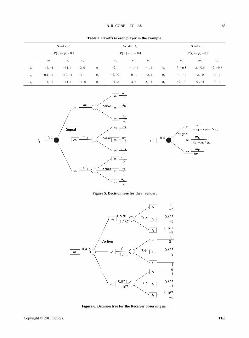
nd category. payoffs and prior probabilities for Sen

he

each pair is the payoff to the R econd num

lection phas als ist and

m

k,

es to itate the determinatio of an equ n the seco

The der type in the game are listed in Table 2. T Sender may be one of three types and the Receiver has three possible actions. The first number in

eceiver and the s ber is the payoff to the Sender.

In this problem, calculating a or m in the strategy se e reve purely mixed Nash that a

doequilibrium does not ex minated strategies must be identified to determine the Nash equilibrium. The procedure fro Section 4 gives the solutions 11 3.237a ,

1.15 1.082a as the strategies for the 12 13

Rece ing 1m6a

iver obs, and erv . Clearly, these are

babilities and this result provides an indication that the Sender has a dominated strategy.

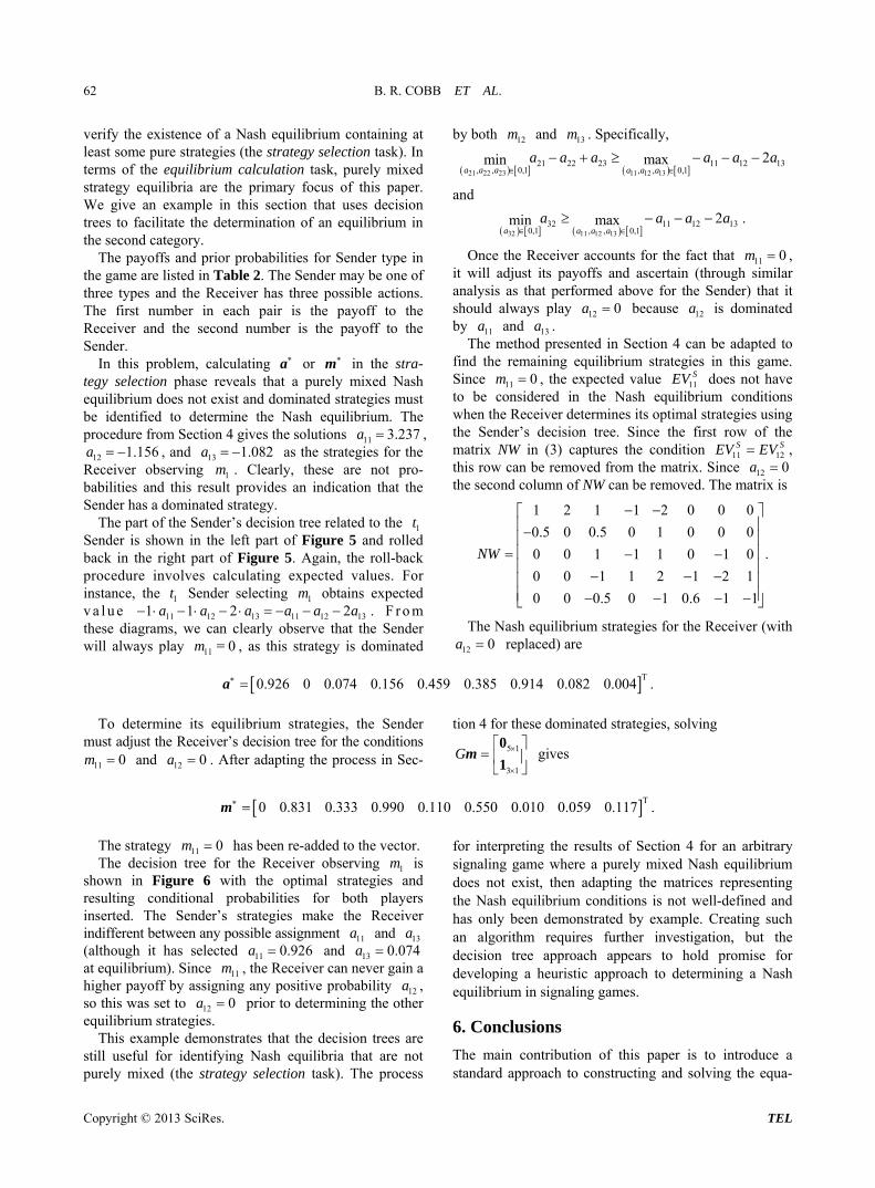
The part of the Sender’s decision tree related to th 1 Se Figure 5 and roback in the right part of Figure 5. Again, the roll-b ck procedure involves calculating expected values. instance, the Sender selecting o s expv a l u e . F r m these w

th

not pro-

by bo 12m and 13m . Specifically,

21 22 23 11 12 1321 22 23 11 12 13

, , 0,1 , , 0,12maxmin

a a a a a aa a a a a a

and

32 11 12 132 .maxmin a a a a

32 11 12 130,1 , , 0,1a a a a

Once the Receiver accounts for the fact that 11 0m , it will adjust its payoffs and ascertain (through similar analysis as that performed above for the Sender) that it should always play 12 0a because 12a is dominated by 11a and 13a .

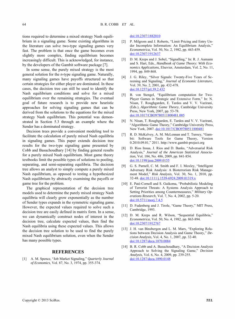
The method presented in Section be o fin

4 can adapted td the remaining equilibrium strategies in this game.

Since 11 0m , the expected value 11SEV does not have

to be considered in the Nash equilibrium conditions when the Receiver determines its optimal strategies using the Sender’s decision tree. Since the first row of the matrix N S SW in (3) captures th e

the condition m .

11 12EV EVS

, is row can be removed from th atrix ince 12 0a

the second column of NW can be removed. The matrix is

1 2 1 1 2 0 0 0

0.5 0 0.5 0 1 0 0 0

.0 0 1 1 0

0 0 1 1 2 2 1

0 0 0.5 0 1 0.6 1 1

e tlled aFor

ected o

nder

nder is shown in the left part of 1 0 1

1

NW

1t

11

s

1m

11a r

s

btain

12 13 12 131 1 2 2a a a a a diagram , we can clearly obse ve that the Se

m s The Nash equilibrium strategies for the Receiver (with

12 0a replaced) are

T0.385 0.914 0.082 0.004 .

tion 4 for these dominated strategies, solving

5 1G

ill always play 11 = 0 , as thi trategy is dominated

0.926 0 0.074 0.156 a 0.459

To determine its equilibrium strategies, the Sender

must adjust the Receiver’s decision tree for the conditions and . After adapting the process in Sec- 11 0m 12 0a

3 1

m0

1 gives

ha -aobserving is

sh it opot

(a

T0 0.831 0.333 0.990 0.110 0.550 0.010 0.059 0.117 . m

The strategy 11 0m s been re dded to the vector. The decision tree for the Receiver 1

own in Figure 6 w h the timal strategies and resulting conditional probabilities for binserted. The Sender’s strategies make the Receiver indifferent between any possible assignment a

m

h players

and 11 13

lthough it has selected 11 0.926aa

and 13 0.074a at equilibrium). Since 11m , the Receiver can never gain a higher payoff by assigning any positive probability , so this was set to 12 0a

12

r a

he othe prior to determeq

nopurely mixed (the strategy selection task). The process

for interpreting the results of Section 4 for an arbitrary signaling game where a purely mixed Nash equilibrium does not exist, then adapting the matrices representing the Nash equilibrium conditions is not well-defined and has only been demonstrated by example. Creating such an algorithm requires further investigation, but the decision tree approach appears to hold promise for developing a heuristic approach to determining a Nash equilibrium in signaling games.

6. Conclusions

The main contribution of this paper is to introduce a standard approach to constructing and solving the equa-

ining tuilibrium strategies. This example demonstrates that the decision trees are

still useful for identifying Nash equilibria that are t


Table 2. Payoffs to each p

Sender Sen

layer in the example.

der 2t Sender 3t 1t

1 1 0.4P t p 2P t 2 0.4p 3 3 0.2P t p

1m 2

1m 2m 3m m 3m

1m 2m 3m

1 1a −2, −1 − 1 − − 6 11, 1 2, 0 a −2, 1 −1, − 1, 1 1a 3, −0.5 2, −0.5 2, −0.

2a 0.1, −1 −10, −1 −1, 1 2a −2, 0

3a −1, −2 −11, 1 −1, 0 3a −1, 2

0 , 1 −2, 2 −1, −1 −2, −1, 1

4, 2 2, −1 −2, −1 −3,

2a 0

3a 0 0 , 1

for the t1 Sender. Figure 5. Decision tr

ee

Figure 6. Decision tree for the Receiver observing m1.



tions required to determine a mixed strategy Nash equilibrium in a signaling game. Some existing algorithms in the literature can solve two-type signaling games very fast. The problem is that once the game becomes even slightly more complex, finding equilibrium becomes increasingly difficult. This is acknowledged, for instance, by the developers of the Gambit software package [7].

In some sense, the purely mixed strategy is the most general solution for the n-type signaling game. Naturally, many signaling games have payoffs structured so that certain strategies for either player are dominated. In these cases, the decision tree can still be used to identify the Nash equilibrium conditions and solve for a mixed equilibrium over the remaining strategies. The eventual goal of future research is to provide new heuristic approaches for solving signaling games that can be derived from the solutions to the equations for the mixed strategy Nash equilibrium. This potential was demonstrated in Section 5.3 through an example where the Sender has a dominated strategy.

Decision trees provide a convenient acilitate the calculation of purely mixed Nash equilibria

in signaling games. This paper extends decision tree results for the two-type signaling game presented by Cobb and Basuchoudhary [14] by finding general results for a purely mixed Nash equilibrium. Most game theory textbooks limit the possible types of solutions to pooling, separating, and semi-separating equilibria. The decision tree allows an analyst to simply compute a purely mixed Nash equilibrium, as opposed to testing a hypothesized Nash equilibrium by abstractly examining the payoffs or game tree for the problem.

The graphical representation of the decision tree models used to determine the purely mixed strategy Nash equilibria will clearly grow exponentially as the number of Sender types expands in the symmetric signaling game. However, the expected values required to solve such a decision tree are easily defined in matrix form. In a sense, we can dynamically construct nodes of interest in the decision tree, calculate expected values, then find the Nash equilibria using these expected values. This allows the decision tree solution to be used to find the purely mixed Nash equilibrium solution, even when the Sender as many possible types.

doi:10.2307/1882010

[2] P. Milgrom and J. Roberts, “Limit Pricing and Entry Un-der Incomplete Information: An Equilibrium Analysis,” Econometrica, Vol. 50, No. 2, 1982, pp. 443-459. doi:10.2307/1912637

[3] D. M. Kreps and J. Sobel, “Signalling,” In: R. J. Aumann and S. Hart, Eds., Handbook of Game Theory: With Eco-nomics Applications, Elsevier, Amsterdam, Vol. 2, No. 11, 1994, pp. 849-868.

[4] J. G. Riley, “Silver Signals: Twenty-Five Years of Sc- reening and Signaling,” Journal of Economic Literature, Vol. 39, No. 2, 2001, pp. 432-478. doi:10.1257/jel.39.2.432

[5] B. von Stengel, “Equilibrium computation for Two- Player Games in Strategic and Extensive Form,” In: N. Nisan, T. Roughgarden, E. Tardos and V. V. Vazirani, (Eds.), Algorithmic Game Theory, Cambridge University Press, New York, 2007, pp. 53-78. doi:10.1017/CBO9780511800481.005

[6] N. Nisan, T. Roughgarden, E. Tardos and V. V. Vazirani, “Algorithmic Game Theory,” Cambridge University Press,

. doi:10.1017/CBO9780511800481modeling tool to

f

h

REFERENCES [1] A. M. Spence, “Job Market Signaling,” Quarterly Journal

of Economics, Vol. 87, No. 3, 1974, pp. 355-374.

New York, 2007

A. M. McLennan and T. Turocy, “Gam-bit: Software Tools for Game Theory, Version 0.2010.09.01,” 2011. http://www.gambit-project.org

[8] D. Rios Insua, J. Rios and D. Banks, “Adversarial Risk Analysis,” Journal of the American Statistical Associa-tion, Vol. 104, No. 486, 2009, pp. 841-854. doi:10.1198/jasa.2009.0155

[7] R. D. McKelvey,

[9] G. S. Parnell, C. M. Smith and F. I. Moxley, “Intelligent Adversary Risk Analysis: A Bioterrorism Risk Manage-ment Model,” Risk Analysis, Vol. 30, No. 1, 2010, pp. 32-48. doi:10.1111/j.1539-6924.2009.01319.x

[10] E. Paté-Cornell and S. Guikema, “Probabilistic Modeling of Terrorist Threats: A Systems Analysis Approach to Setting Priorities among Countermeasures,” Military Op-erations Research, Vol. 7, No. 4, 2002, pp. 5-20. doi:10.5711/morj.7.4.5

[11] D. Fudenberg and J. Tirole, “Game Theory,” MIT Press, Cambridge, 1993.

[12] D. M. Kreps and R. Wilson, “Sequential Equilibria,” Econometrica, Vol. 50, No. 4, 1982, pp. 863-894. doi:10.2307/1912767

[13] J. H. van Binsbergen and L. M. Marx, “Exploring Rela-tions between Decision An sis and Game Theory,” De-

4, No. 1, 2007, pp. 32-40. aly

cision Analysis, Vol. doi:10.1287/deca.1070.0084

[14] B. R. Cobb and A. Basuchoudhary, “A Decision Analysis Approach to Solving the Signaling Game,” Decision Analysis, Vol. 6, No. 4, 2009, pp. 239-255. doi:10.1287/deca.1090.0148


Documents

Mixed Strategy Nash Equilibria in Signaling Games