Embed Size (px)
Citation preview

The Complexity of Nash Equilibria
Constantinos Daskalakis
Electrical Engineering and Computer SciencesUniversity of California at Berkeley
Technical Report No. UCB/EECS-2008-107
http://www.eecs.berkeley.edu/Pubs/TechRpts/2008/EECS-2008-107.html
August 28, 2008

Copyright 2008, by the author(s).All rights reserved.
Permission to make digital or hard copies of all or part of this work forpersonal or classroom use is granted without fee provided that copies arenot made or distributed for profit or commercial advantage and that copiesbear this notice and the full citation on the first page. To copy otherwise, torepublish, to post on servers or to redistribute to lists, requires prior specificpermission.
The Complexity of Nash Equilibria
by
Constantinos Daskalakis
Diploma (National Technical University of Athens) 2004
A dissertation submitted in partial satisfaction of the
requirements for the degree of
Doctor of Philosophy
in
Computer Science
in the
Graduate Division
of the
University of California, Berkeley
Committee in charge:
Professor Christos H. Papadimitriou, ChairProfessor Alistair J. Sinclair
Professor Satish RaoProfessor Ilan Adler
Fall 2008

The dissertation of Constantinos Daskalakis is approved:
Chair Date
Date
Date
Date
University of California, Berkeley
Fall 2008

The Complexity of Nash Equilibria
Copyright 2008
by
Constantinos Daskalakis
Abstract
The Complexity of Nash Equilibria
by
Constantinos Daskalakis
Doctor of Philosophy in Computer Science
University of California, Berkeley
Professor Christos H. Papadimitriou, Chair
The Internet owes much of its complexity to the large number of entities that run it
and use it. These entities have different and potentially conflicting interests, so their
interactions are strategic in nature. Therefore, to understand these interactions,
concepts from Economics and, most importantly, Game Theory are necessary. An
important such concept is the notion of Nash equilibrium, which provides us with a
rigorous way of predicting the behavior of strategic agents in situations of conflict. But
the credibility of the Nash equilibrium as a framework for behavior-prediction depends
on whether such equilibria are efficiently computable. After all, why should we expect
a group of rational agents to behave in a fashion that requires exponential time to
be computed? Motivated by this question, we study the computational complexity of
the Nash equilibrium.
We show that computing a Nash equilibrium is an intractable problem. Since by
Nash’s theorem a Nash equilibrium always exists, the problem belongs to the family
of total search problems in NP, and previous work establishes that it is unlikely
that such problems are NP-complete. We show instead that the problem is as hard
as solving any Brouwer fixed point computation problem, in a precise complexity-
theoretic sense. The corresponding complexity class is called PPAD, for Polynomial
Parity Argument in Directed graphs, and our precise result is that computing a Nash
1
equilibrium is a PPAD-complete problem.
In view of this hardness result, we are motivated to study the complexity of com-
puting approximate Nash equilibria, with arbitrarily close approximation. In this
regard, we consider a very natural and important class of games, called anonymous
games. These are games in which every player is oblivious to the identities of the
other players; examples arise in auction settings, congestion games, and social inter-
actions. We give a polynomial time approximation scheme for anonymous games with
a bounded number of strategies.
Professor Christos H. Papadimitriou
Dissertation Committee Chair
2

Acknowledgments
Christos once told me that I should think of my Ph.D. research as a walk through a
field of exotic flowers. “You should not focus on the finish line, but enjoy the journey.
And, in the end, you’ll have pollen from all sorts of different flowers on your clothes.”
I want to thank Christos for guiding me through this journey and everyone else who
contributed in making these past four years a wonderful experience.
I first met Christos in Crete, the island in Greece where my family comes from.
Christos was giving a set of talks on Algorithmic Game Theory as part of the Onassis
Foundation science lecture series on the Internet and the Web. I walked into the
amphitheater a bit late, and the first thing I saw was a slide depicting the Internet as
a cloud connecting a dozen of computers. This cloud started growing, and, as it grew,
it devoured the computers and broke out of the boundaries of the screen. Then, a
large question-mark appeared. In the next couple of slides Christos explained Game
Theory and the concept of the Nash equilibrium as a framework for studying the
Internet. I had no idea at that moment that this would be the motivation for my
Ph.D. research. . .
I am indebted to Christos for mentoring me through this journey, and for teaching
me how to look at the essence of things. His belief in me, his enthusiasm, and his
support were essential for me to realize my potential. But I thank him even more for
being there as a friend, for all our discussions over wine at Cesar, and for our cups of
coffee at Nefeli Cafe. I only wish that I will be to my students as great of an advisor
and friend as Christos has been to me.
I also want to thank all my other teachers at Berkeley, above all, the members of
the theory group for the unique, friendly, and stimulating atmosphere they create. I
thank Dick Karp for being a valuable collaborator and advisor and for guiding me
i

through my first experience as a teacher. I will always admire and be inspired by his
remarkable profoundness and simplicity. I thank Satish Rao for his support through
the difficult time of choosing a research identity, for stimulating political discussions,
and for our amusing basketball and soccer games. I thank Alistair Sinclair for his ran-
domness and computation class, and his helpful guidance and advice. I thank Luca
Trevisan for the complexity theory that he taught me and Umesh Vazirani for his
unique character and spirit. Thanks to Ilan Adler for serving in my dissertation com-
mittee and to Tandy Warnow for involving me in CIPRES. Finally, many thanks are
due to Elchanan Mossel, who has been a valuable collaborator and a great influence in
turning my research interests towards the applications of Probability Theory in Com-
puter Science and Biology. I thank him for the hours we spent thinking together, his
inexhaustible enthusiasm, and his support.
I feel indebted to all my collaborators: Christos, Dick, Elchanan, Satish, Christian
Borgs, Jennifer Chayes, Kamalika Chaudhuri, Alexandros Dimakis, Alex Fabrikant,
Paul Goldberg, Cameron Hill, Alex Jaffe, Robert Kleinberg, Henry Lin, Aranyak
Mehta, Radu Mihaescu, Samantha Riesenfeld, Sebastien Roch, Grant Schoenebeck,
Gregory and Paul Valiant, Elad Verbin, Martin J. Wainwright, Dimitris Achlioptas,
Sanjeev Arora, Arash Asadpour, Albert Atserias, Omid Etesami, Jason Hartline,
Nicole Immorlica, Elias Koutsoupias, David Steurer, Shanghua Teng, Adrian Vetta,
and Riccardo Zecchina. Thanks for the hours we spent thinking together, and the
unique things I learned from each of you!
Thanks also to all the students in Berkeley’s Computer Science, Electrical En-
gineering and Statistics departments for four wonderful years. Special thanks to
Alex Dimakis, Omid Etesami, Slav Petrov, Sam Riesenfeld, Grant Schoenebeck, Ku-
nal Talwar, Andrej Bogdanov, Alex Fabrikant, Simone Gambini, Brighten Godfrey,
Alexandra Kolla, James Lee, Henry Lin, Mani Narayanan, Lorenzo Orrechia, Boriska
Toth and Madhur Tulsiani. Thanks to Alex, Omid, Sam and Slav for being valuable
ii

friends. Thanks to Grant for a great China trip. Thanks to Alex, Omid and Slav for
a wonderful road-trip in Oregon. And thanks to Alexandra and Slav for an amazing
Costa Rica trip. Also, thanks to all students in the theory group for our Lake Tahoe
retreat.
Outside of Berkley I feel very grateful towards Elias Koutsoupias, Timos Sellis and
Stathis Zachos. I am grateful to Stathis for introducing me to theoretical computer
science during my undergraduate studies and for turning my research interests towards
the theory of computation. I thank Timos for being a wonderful advisor and friend
back in my undergraduate years and Elias for being a good friend and great influence
throughout my Ph.D. years.
I want to thank UC Berkeley, NSF, CIPRES, Microsoft and Yahoo! for support-
ing my research. I especially thank UC Regents for the fellowship I received my
first year and Microsoft Research for the Graduate Research Fellowship I received
my last year. I also thank Microsoft Research for two productive summer intern-
ships. Special thanks are due to my mentors Jennifer Chayes and Christian Borgs
for being extremely supportive during my time as an intern and for their continuing
appreciation and support.
I also feel deeply honored by the Game Theory and Computer Science prize that
the Game Theory Society awarded to my collaborators and me for our research on
the Complexity of Nash equilibria. Their appreciation of our research is extremely
gratifying.
I want to thank the Greeks of the Bay Area for their friendship and support. Spe-
cial thanks to Maria-Daphne, Constantinos, Manolis, Lefteris, Alexandros, Alexan-
dra, George, Dimitris, Stergios, Christos, Tasos, Apostolis, Katerina, Eleni, Antonis
and Antonis. Maria-Daphne, Lefteri and Alexandre, thanks for a wonderful Mexico
trip. Costa, Manoli and Antoni, I will never forget our trip to Hawaii.
Thanks also to Ilias, Natassa, Maria-Daphne, Aliki, Nikos, Nicole, Jason, Alisar
iii

and Alexandra C. I am grateful to each of you for being in my life, for all your love
and support.
Thanks to Berkeley itself for its magical ambience. I am grateful for all the mo-
ments I spent at Cafe Strada, Nefeli Cafe, Brewed Awakening, Cesar, the i-House,
and the French Hotel Cafe. I also cannot forget the beautiful sunsets at the Theology
School between Le Conte and Arch Streets.
Last but not least, I am grateful to my family. I have no way to thank them for
their invaluable presence in my life, my memories, my whole essence, but to dedicate
this dissertation to them.
iv

To my parents Pericles and Sophia for inspiring my love for knowledge,
and to my brother Nikos for sharing this journey with me.
v
Contents
1 Introduction 1
1.1 Games and the Theory of Games . . . . . . . . . . . . . . . . . . . . 2
1.2 The History of the Nash Equilibrium . . . . . . . . . . . . . . . . . . 6
1.3 Overview of Results . . . . . . . . . . . . . . . . . . . . . . . . . . . . 11
1.4 Discussion of Techniques . . . . . . . . . . . . . . . . . . . . . . . . . 15
1.5 Organization of the Dissertation . . . . . . . . . . . . . . . . . . . . . 19
2 Background 21
2.1 Basic Definitions from Game Theory . . . . . . . . . . . . . . . . . . 22
2.2 The Complexity Theory of Total Search Problems and the Class PPAD 25
2.3 Computing a Nash Equilibrium is in PPAD . . . . . . . . . . . . . . 27
2.4 Brouwer: a PPAD-Complete Fixed Point Computation Problem . . 40
2.5 Related Work on Computing Nash Equilibria and Other Fixed Points 48
3 Reductions Among Equilibrium Problems 50
3.1 Preliminaries: Game Gadgets . . . . . . . . . . . . . . . . . . . . . . 51
3.2 Reducing Graphical Games to Normal-Form Games . . . . . . . . . . 58
3.3 Reducing Normal-Form Games to Graphical Games . . . . . . . . . . 65
3.4 Combining the Reductions . . . . . . . . . . . . . . . . . . . . . . . . 74
3.5 Reducing to Three Players . . . . . . . . . . . . . . . . . . . . . . . . 77
vi
3.6 Preservation of Approximate equilibria . . . . . . . . . . . . . . . . . 84
3.7 Reductions Between Different Notions of Approximation . . . . . . . 99
4 The Complexity of Computing a Nash Equilibrium 103
4.1 The Complexity of Games with Three or More Players . . . . . . . . 104
4.2 Two-Player Games . . . . . . . . . . . . . . . . . . . . . . . . . . . . 118
4.3 Other Classes of Games and Fixed Points . . . . . . . . . . . . . . . . 123
5 Computing Approximate Equilibria 126
5.1 General Games and Special Classes . . . . . . . . . . . . . . . . . . . 127
5.2 Anonymous Games . . . . . . . . . . . . . . . . . . . . . . . . . . . . 131
5.3 Definitions and Notation . . . . . . . . . . . . . . . . . . . . . . . . . 133
5.4 A Polynomial-Time Approximation Scheme for Anonymous Games . 134
5.5 An Approximation Theorem for Multinomial Distributions . . . . . . 136
5.6 Discussion of Proof Techniques . . . . . . . . . . . . . . . . . . . . . 140
5.7 Proof of the Multinomial Approximation Theorem . . . . . . . . . . . 142
5.7.1 The Trickle-Down Process . . . . . . . . . . . . . . . . . . . . 142
5.7.2 An Alternative Sampling of the Random Vectors . . . . . . . . 144
5.7.3 Clustering the Random Vectors . . . . . . . . . . . . . . . . . 144
5.7.4 Discretization within a Cell of the Clustering . . . . . . . . . . 145
5.7.5 Coupling within a Cell of the Clustering . . . . . . . . . . . . 146
5.7.6 Total Variation Distance within a Leaf . . . . . . . . . . . . . 149
5.8 Extensions . . . . . . . . . . . . . . . . . . . . . . . . . . . . . . . . . 152
5.9 Towards Efficient Polynomial-Time Approximation Schemes . . . . . 153
6 Conclusions and Open Problems 155
A Skipped Proofs 171
A.1 Proof of Lemma 5.9 . . . . . . . . . . . . . . . . . . . . . . . . . . . . 173
vii

A.2 Proof of Lemma 5.10 . . . . . . . . . . . . . . . . . . . . . . . . . . . 179
A.3 Concentration of the Leaf Experiments . . . . . . . . . . . . . . . . . 184
viii

List of Figures
1.1 The Railroad Crossing Game . . . . . . . . . . . . . . . . . . . . . . . 3
1.2 The Penalty Shot Game . . . . . . . . . . . . . . . . . . . . . . . . . 5
2.1 The orthonormal path connecting vertices (u,v); the arrows indicate
the orientation of colors surrounding the path. . . . . . . . . . . . . . 43
2.2 The 27 cubelets around the beginning of line L. . . . . . . . . . . . . 45
3.1 G×α, G= . . . . . . . . . . . . . . . . . . . . . . . . . . . . . . . . . . 53
3.2 Gα . . . . . . . . . . . . . . . . . . . . . . . . . . . . . . . . . . . . . 53
3.3 G+,G∗,G− . . . . . . . . . . . . . . . . . . . . . . . . . . . . . . . . . . 53
3.4 Gmax . . . . . . . . . . . . . . . . . . . . . . . . . . . . . . . . . . . . 56
3.5 Reduction from the graphical game GG to the normal-form game G . 59
3.6 Diagram of Proposition 3.13 . . . . . . . . . . . . . . . . . . . . . . . 68
3.7 Reduction from normal-form game G to graphical game GG . . . . . . 71
3.8 Reduction from normal-form game G to 4-player game G′ . . . . . . . 76
3.9 The new addition/multiplication game and its legal 3-coloring. . . . . 78
3.10 The interposition of two G= games between gadgets G1 and G2 does not
change the game. . . . . . . . . . . . . . . . . . . . . . . . . . . . . . 83
4.1 Brittleness of Comparator Games. . . . . . . . . . . . . . . . . . . . . 106
ix
Chapter 1
Introduction
Do we understand the Internet? One possible response to this question is “Of course
we do, since it is an engineered system”. Indeed, at the very least, we do understand
the design of its basic components and the very basic processes running on them. On
the other hand, we are often surprised by singular events that occur on the Internet: in
February 2008, for example, a mere Border Gateway Protocol (BGP) table update in
a network in Pakistan resulted in a two-hour outage of YouTube accesses throughout
the globe. . .
What we certainly understand is that the Internet is a remarkably complex system.
And it owes much of its complexity to the large number of entities that run it and
use it, through such familiar applications as routing, file sharing, online advertising,
and social networking. These interactions occurring in the Internet, much like those
happening in social and biological systems, are often strategic in nature, since the
participating entities have different and potentially conflicting interests. Hence, to
understand the Internet, it makes sense to use concepts and ideas from Economics
and, most importantly, Game Theory.
One of Game Theory’s most basic and influential concepts, which provides us with
a rigorous way of describing the behaviors that may arise in a system of interacting
1

agents, is the concept of the Nash equilibrium. And this dissertation is devoted to
the study of the computational complexity of the Nash equilibrium. But why consider
computational complexity? First, it is a very natural and useful question to answer.
Second, because of the computational nature of the motivating application, it is
natural to study the computational aspects of the concepts we introduce for its study.
But the main justification for this question is philosophical: Equilibria are models of
behavior of rational agents, and, as such, they should be efficiently computable. After
all, it is doubtful that groups of rational agents are computationally more powerful
than computers; and, if they were, it would be really remarkable. Hence, whether
equilibria are efficiently computable is a question of fundamental significance for Game
Theory, the field for which equilibrium is perhaps the most central concept.
1.1 Games and the Theory of Games
Game Theory is one of the most important and vibrant mathematical fields estab-
lished in the 20th century. It studies the behavior of strategic agents in situations of
conflict, called games; these, e.g., include markets, transportation networks, and the
Internet.
• But how is a game modeled mathematically?
A game can be described by naming its players and specifying the strategies
available to them. Then, for every selection of strategies by the players, each of
them gets some (potentially negative) utility, called payoff. The payoffs can be given
implicitly as functions of the players’ strategies; or, if the number of strategies is
finite, they can be given explicitly by tables.
For example, Figure 1.1 depicts a variant of the Chicken Game [OR94], called
the Railroad Crossing Game: A car and a train approach an unprotected railroad
crossing at collision speed. If both the car driver and the train operator choose to
2
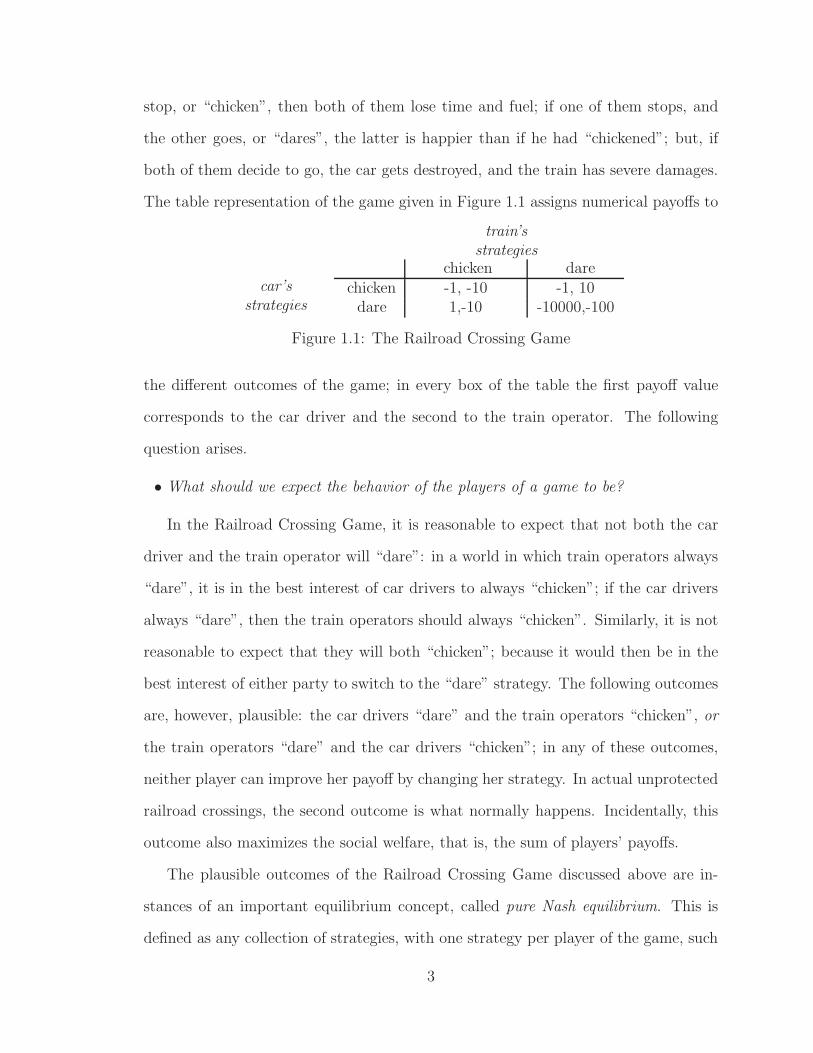
stop, or “chicken”, then both of them lose time and fuel; if one of them stops, and
the other goes, or “dares”, the latter is happier than if he had “chickened”; but, if
both of them decide to go, the car gets destroyed, and the train has severe damages.
The table representation of the game given in Figure 1.1 assigns numerical payoffs to
train’sstrategies
car’sstrategies
chicken darechicken -1, -10 -1, 10
dare 1,-10 -10000,-100
Figure 1.1: The Railroad Crossing Game
the different outcomes of the game; in every box of the table the first payoff value
corresponds to the car driver and the second to the train operator. The following
question arises.
• What should we expect the behavior of the players of a game to be?
In the Railroad Crossing Game, it is reasonable to expect that not both the car
driver and the train operator will “dare”: in a world in which train operators always
“dare”, it is in the best interest of car drivers to always “chicken”; if the car drivers
always “dare”, then the train operators should always “chicken”. Similarly, it is not
reasonable to expect that they will both “chicken”; because it would then be in the
best interest of either party to switch to the “dare” strategy. The following outcomes
are, however, plausible: the car drivers “dare” and the train operators “chicken”, or
the train operators “dare” and the car drivers “chicken”; in any of these outcomes,
neither player can improve her payoff by changing her strategy. In actual unprotected
railroad crossings, the second outcome is what normally happens. Incidentally, this
outcome also maximizes the social welfare, that is, the sum of players’ payoffs.
The plausible outcomes of the Railroad Crossing Game discussed above are in-
stances of an important equilibrium concept, called pure Nash equilibrium. This is
defined as any collection of strategies, with one strategy per player of the game, such
3

that, given the strategies of the other players, none of them can improve their payoff
by switching to a different strategy. Hence, it is reasonable for every player to stick
to the strategy prescribed to her.
To understand the pure Nash equilibrium as a concept of behavior prediction,
let us adopt the following interpretation of a game, called the steady state interpre-
tation: 1 We view a game as a model designed to explain some regularity observed
in a family of similar situations. A player of the game forms her expectation about
the other players’ behavior on the basis of the information about how the game or a
similar game was played in the past. That is, every player “knows” the equilibrium of
the game that she is about to play and only tests the optimality of her behavior given
this knowledge; and the pure Nash equilibrium specifies exactly the conditions that
need to hold so that she does not need to adopt a different behavior. Observe that
the steady state interpretation is what we used to argue about the equilibria of the
Railroad Crossing Game: we viewed the game as a model of the interaction between
two populations, the train operators and the car drivers, and each instance of the
game took place when two members of these populations met at a railroad crossing.
It is important to note that the pure Nash equilibrium is a convincing method of
behavior-prediction only in the absence of strategic links between the different plays
of the game. If there are inter-temporal strategic links between occurrences of the
game, different equilibrium concepts are necessary.
The pure Nash equilibrium is a simple and convincing equilibrium concept. Alas,
it does not exist in every game. Let us consider, for example, the Penalty Shot Game
described in Figure 1.2. The numerical values in the table specify the following rules:
if the goalkeeper and the penalty kicker choose the same strategy, then the goalkeeper
wins a point, and the penalty kicker loses a point; if they choose different strategies,
then the goalie loses, and the penalty kicker wins. Observe that there is no pure Nash
1See, e.g., Osborne and Rubinstein [OR94] for a more detailed discussion of the subject.
4
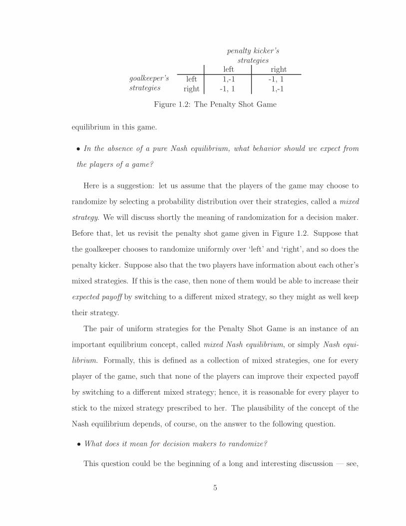
penalty kicker’sstrategies
goalkeeper’sstrategies
left rightleft 1,-1 -1, 1
right -1, 1 1,-1
Figure 1.2: The Penalty Shot Game
equilibrium in this game.
• In the absence of a pure Nash equilibrium, what behavior should we expect from
the players of a game?
Here is a suggestion: let us assume that the players of the game may choose to
randomize by selecting a probability distribution over their strategies, called a mixed
strategy. We will discuss shortly the meaning of randomization for a decision maker.
Before that, let us revisit the penalty shot game given in Figure 1.2. Suppose that
the goalkeeper chooses to randomize uniformly over ‘left’ and ‘right’, and so does the
penalty kicker. Suppose also that the two players have information about each other’s
mixed strategies. If this is the case, then none of them would be able to increase their
expected payoff by switching to a different mixed strategy, so they might as well keep
their strategy.
The pair of uniform strategies for the Penalty Shot Game is an instance of an
important equilibrium concept, called mixed Nash equilibrium, or simply Nash equi-
librium. Formally, this is defined as a collection of mixed strategies, one for every
player of the game, such that none of the players can improve their expected payoff
by switching to a different mixed strategy; hence, it is reasonable for every player to
stick to the mixed strategy prescribed to her. The plausibility of the concept of the
Nash equilibrium depends, of course, on the answer to the following question.
• What does it mean for decision makers to randomize?
This question could be the beginning of a long and interesting discussion — see,
5
e.g., Osborne and Rubinstein [OR94] for a detailed analysis. So, we only attempt
an explanation here. To do this we revisit the steady state interpretation of a game,
according to which a game models an environment in which players act repeatedly and
ignore strategic links between different plays. By the same token, we can interpret
the Nash equilibrium as a stochastic steady state as follows: Each player of the
game collects statistical data about the frequencies with which different actions were
taken in the previous plays of the game. And she chooses an action according to the
beliefs she forms about the other players’ strategies from these statistics. The Nash
equilibrium then describes the frequencies with which different actions are played by
the players of the game in the long run. Coming back to the Penalty Shot Game, it is
reasonable to expect that in half of the penalty shots played in this year’s EuroCup
the penalty kicker shot right and in half of them the goalkeeper dived left.
The pure Nash equilibrium is of course more attractive than the mixed Nash
equilibrium, since it does not require the players to randomize. However, as noted
above, it does not exist in every game, and this makes its value as a framework for
behavior prediction rather questionable. For the same reason, the usefulness and
plausibility of the mixed Nash equilibrium is contingent upon a positive answer to
the following question.
• Is there a mixed Nash equilibrium in every game?
1.2 The History of the Nash Equilibrium
In 1928, John von Neumann, extending work by Emile Borel, showed that any two-
player zero-sum game — that is, a game in which every outcome has zero payoff-sum,
such as the Penalty Shot Game of Figure 1.2 — has a mixed equilibrium [Neu28].
Two decades after von Neumann’s result it was understood that the existence of an
equilibrium in zero-sum games is equivalent to Linear Programming duality [AR86,
6
Dan63], and, as was established another three decades later [Kha79], finding such an
equilibrium is computationally tractable. In other words, computationally speaking,
the state of affairs of equilibria in zero-sum games is quite satisfactory.
However, as it became clear with the seminal book by von Neumann and Morgen-
stern [NM44], zero-sum games are too specialized and fail to capture most interesting
situations of conflict between rational strategic players. Hence, the following question
became important.
• Is there a Nash equilibrium in non-zero-sum multi-player games?
The answer to this question came in 1951 with John Nash’s important and deeply
influential result: every game, independent of the number of players and strategies
available to them (provided only that these numbers are finite) and of the proper-
ties of the players’ payoffs, has an equilibrium in randomized strategies, henceforth
called a Nash equilibrium [Nas51]. Nash’s proof, based on Brouwer’s fixed point the-
orem [KKM29] is mathematically beautiful, but non-constructive. Even the more re-
cent combinatorial proofs of Brouwer’s fixed point theorem based on Sperner’s lemma
(see, e.g., Papadimitriou [Pap94b]) result in exponential time algorithms. Due to the
importance of the Nash equilibrium concept, soon after Nash’s result the following
question emerged.
• Are there efficient algorithms for computing a Nash equilibrium?
We will consider this question in the centralized model of computation. Of course,
the computations performed by strategic agents during game-play are modeled more
faithfully by distributed protocols; and these protocols should be of a very special
kind, since they correspond to rational behavior of strategic agents. 2 Hence, it is
not clear a priori whether an efficient centralized algorithm for computing a Nash
equilibrium would imply a natural and efficient distributed protocol for the same
2The reader is referred to Fudenberg and Levine [FL99] for an extensive discussion of naturalprotocols for game-play.
7
task. However, it is true — and will be of central importance for the philosophical
implications of our results discussed in Section 1.3 — that an intractability result for
centralized algorithms implies a similar result for distributed algorithms. After all,
the computational parallelism, inherent in the interaction of players during game-play,
can only result in polynomial-time speedups.
Whether Nash equilibria can be computed efficiently has been studied extensively
in the Economics and Optimization literature. At least for the two-player case, the
hope for a positive answer was supported by a remarkable similarity of the problem
to linear programming: there always exist rational solutions, and the Lemke-Howson
algorithm [LH64], a simplex-like technique for solving two-player games, appears to be
very efficient in practice. There are generalizations of the Lemke-Howson algorithm
applying to the multi-player case [Ros71, Wil71]; however, as noted by Nash in his
original paper [Nas51], there are three-player games with only irrational equilibria.
This gives rise to the following question.
• What does it mean to compute a Nash equilibrium in the presence of irrational
equilibria?
There are two obvious ways to define the problem: One is to ask for a collection of
mixed strategies within a specified distance from a Nash equilibrium. And the other
is to ask for mixed strategies such that no player has more than some (small) specified
incentive to change her strategy; that is, a collection of mixed strategies such that
every player is playing an approximate best response to the other players’ strategies.
The latter notion of approximation is arguably more natural for applications (since
the players’ goal in a game is to optimize their payoffs rather than the distance of their
strategies from an equilibrium strategy), and we are going to adopt this notion in this
dissertation. This is also the standard notion used in the literature of algorithms for
equilibria, e.g., those based on the computation of fixed points [Sca67, Eav72, GLL73,
8
LT79]. For the former notion of approximation, the reader is referred to the recent
work of Etessami and Yannakakis [EY07].
Despite extensive research on the subject, none of the existing algorithms for
computing Nash equilibria are known to be efficient. There are instead negative
results [HPV89], most notably for the Lemke-Howson algorithm [SS04]. This brings
about the following question.
• Is computing a Nash equilibrium an inherently hard computational problem?
Besides Game Theory, the 20th century saw the development of another great
mathematical field of tremendous growth and impact, whose concepts enable us to
answer questions of this sort: Computational Complexity. However, the mainstream
concepts and techniques developed by complexity theorists — chief among them NP-
completeness — are not directly applicable for fathoming the complexity of the Nash
equilibrium. There are versions of the problem which are NP-complete, for example
counting the number of equilibria, or deciding whether there are equilibria with certain
properties [GZ89, CS03]. But answering these questions appears computationally
harder than finding a (single) Nash equilibrium. So, it seems quite plausible that the
Nash equilibrium problem could be easier than an NP-complete problem.
The heart of the complication in characterizing the complexity of the Nash equi-
librium is ironically Nash’s Theorem: NP-complete problems seem to draw much of
their difficulty from the possibility that a solution may not exist; and, since a Nash
equilibrium is always guaranteed to exist, NP-completeness does not seem useful in
characterizing the complexity of finding one. What would a reduction from Satisfi-
ability to Nash (the problem of finding a Nash equilibrium) look like? Any obvious
attempt to define such a reduction quickly leads to NP = coNP [MP91]. Hence, the
following question arises.
• If not NP-hard, exactly how hard is it to compute a Nash equilibrium?
9
Motivated mainly by this question for the Nash equilibrium, Meggido and Pa-
padimitriou [MP91] defined in the 1980s the complexity class TFNP (for “NP total
functions”), consisting exactly of all search problems in NP for which every instance is
guaranteed to have a solution. Nash of course belongs there, and so do many other
important and natural problems, finitary versions of Brouwer’s problem included.
But here there is a difficulty of a different sort: TFNP is a “semantic class” [Pap94a],
meaning that there is no easy way of recognizing nondeterministic Turing machines
which define problems in TFNP — in fact the problem is undecidable; such classes
are known to be devoid of complete problems.
To capture the complexity of Nash and other important problems in TFNP,
another step is needed: One has to group together into subclasses of TFNP total
functions whose proofs of totality are similar. Most of these proofs work by essentially
constructing an exponentially large graph on the solution space (with edges that are
computed by some algorithm), and then applying a simple graph-theoretic lemma
establishing the existence of a particular kind of node. The node whose existence is
guaranteed by the lemma is the desired solution of the given instance. Interestingly,
essentially all known problems in TFNP can be shown total by one of the following
arguments:
- In any dag there must be a sink. The corresponding class, PLS for “Polyno-
mial Local Search”, had already been defined in [JPY88] and contains many
important complete problems.
- In any directed graph with outdegree one and with one node with indegree zero,
there must be a node with indegree at least two. The corresponding class is PPP
(for “Polynomial Pigeonhole Principle”).
- In any undirected graph with one odd-degree node, there must be another odd-
degree node. This defines a class called PPA for “Polynomial Parity Argu-
10
ment” [Pap94b], containing many important combinatorial problems (unfortu-
nately none of them known to be complete).
- In any directed graph with one unbalanced node (node with outdegree different
from its indegree), there must be another unbalanced node. The corresponding
class is called PPAD for “Polynomial Parity Argument for Directed graphs,”
and it contains Nash, Brouwer, and Borsuk-Ulam (finding approximate
fixed points of the kind guaranteed by Brouwer’s Theorem and the Borsuk-Ulam
Theorem, respectively, see [Pap94b]). The latter two were among the problems
proven PPAD-complete in [Pap94b]. Unfortunately, Nash — the one problem
which had motivated this line of research — was not shown PPAD-complete; it
was conjectured that it is.
The central question arising from this line of research, and the starting point of this
dissertation, is the following.
• Is computing a Nash equilibrium PPAD-complete?
1.3 Overview of Results
Our main result is that Nash, the problem of computing a Nash equilibrium, is PPAD-
complete. Hence, we settle the questions about the computational complexity of the
Nash equilibrium problem discussed in Section 1.2.
The proof of our main result is presented in Chapter 4. Our original argument
(Section 4.1) works for games with three players or more, leaving open the question
for two-player games. This case was thought to be computationally easier, since, as
discussed in Section 1.2, linear programming-like techniques come into play, and solu-
tions consisting of rational numbers are guaranteed to exist [LH64]; on the contrary,
as exhibited in Nash’s original paper [Nas51], there are three-player games with only
11

irrational equilibria. Surprisingly, a few months after our result was circulated, Chen
and Deng extended our hardness result to the two-player case [CD05, CD06]. In
Section 4.2, we present a simple modification of our argument which also establishes
the hardness of two-player games.
• So, what is the implication of our PPAD-hardness result for Nash equilibria?
First of all, a polynomial-time algorithm for computing Nash equilibria would im-
ply a polynomial-time algorithm for computing Brouwer fixed points of (succinctly de-
scribed) continuous and piece-wise linear functions, a problem for which quite strong
lower bounds for large classes of algorithms are known [HPV89]. Moreover, there are
oracles — that is, computational universes [Pap94a] — relative to which PPAD is
different from P [BCE+98]. Hence, a polynomial-time algorithm for computing Nash
equilibria would have to fail to relativize with respect to these oracles, which seems
unlikely.
Our result gives an affirmative answer to another important question arising from
Nash’s Theorem, namely, whether the reliance of its proof on Brouwer’s fixed point
theorem is inherent. Our proof is essentially a reduction in the opposite direc-
tion to Nash’s: an appropriately discretized and stylized PPAD-complete version
of Brouwer’s fixed point problem in 3 dimensions is reduced to Nash.
In fact, it is possible to eliminate the computational ingredient in this reduction
to obtain a purely mathematical statement, establishing the equivalence between the
existence of a Nash equilibrium in 2- and 3-player games and the existence of fixed
points in continuous piecewise-linear and polynomial maps respectively. This im-
portant point is discussed briefly in Section 4.3 and explored in detail by Etessami
and Yannakakis [EY07]. Mainly due to this realization, we have been able to show
that a large class of equilibrium-computation problems belongs to the class PPAD; in
particular, we can show this for all games for which, loosely speaking, the expected
12
utility of a player can be computed by an arithmetic circuit3 given the other play-
ers’ mixed strategies [DFP06]. In the same spirit, Etessami and Yannakakis [EY07]
relate the computation of Nash equilibria to computational problems, such as the
square-root-sum problem (see, e.g., [GGJ76, Pap77]) and the value of simple stochas-
tic games [Con92], the complexity of which is largely unknown.
But perhaps the most important implication of our result is a critique of the Nash
equilibrium as a framework of behavior prediction — contingent, of course, upon the
hardness of the class PPAD: Should we expect that the players of a game behave in a
fashion which is too expensive computationally? Or, relative also to the steady state
interpretation of a game, is it interesting to study a notion of player behavior which
could only arise after a prohibitively large number of game-plays? In view of these
objections, the following question becomes important.
• In the absence of efficient algorithms for computing a Nash equilibrium, are there
efficient algorithms for computing an approximate Nash equilibrium?
As discussed in the previous section, we are interested in collections of mixed
strategies such that no player has more than some small, say ǫ, incentive to change her
strategy. Let us call such a collection an ǫ-approximate Nash equilibrium. From our
result on the hardness of computing a Nash equilibrium, it follows that, if ǫ is inverse
exponential in the size of the game, computing an ǫ-approximate Nash equilibrium
is PPAD-complete. In fact, this hardness result was extended to the case where
ǫ is inverse polynomial in the size of the game by Chen, Deng and Teng [CDT06a].
Hence, a fully polynomial-time approximation scheme seems unlikely. 4 The following
question then emerges at the boundary of intractability.
3Arithmetic Circuits are analogous to Boolean Circuits, but instead of the Boolean operators∧,∨,¬, they use the arithmetic operators +,−,×.
4A polynomial-time approximation scheme, or PTAS, is a family of approximation algorithms,running in time polynomial in the problem size, for every fixed value of the approximation ǫ. If therunning time is also polynomial in 1/ǫ, the family is called a fully polynomial-time approximation
scheme, or FPTAS.
13
• Is there a polynomial-time approximation scheme for the Nash equilibrium prob-
lem? And, in any case, what would the existence of such a PTAS imply for the
predictive power of the Nash equilibrium?
In view of our hardness result for the Nash equilibrium problem, a PTAS would
be rather important, since it would support the following interpretation of the Nash
equilibrium as a framework for behavior prediction: Although it might take a long
time to approach an exact Nash equilibrium, the game-play could converge — after
a polynomial number of iterations — to a state where all players’ regret is no more
than ǫ, for any desired ǫ. If that ǫ is smaller than the numerical error (e.g., the
quantization of the currency used by the players), then ǫ-regret might not even be
visible to the players.
There has been a significant body of research devoted to the computation of
approximate Nash equilibria [LMM03, KPS06, DMP06, FNS07, DMP07, BBM07,
TS07], however no PTAS is known to date. We discuss the known results in detail in
Chapter 5. Let us only note here that, even for the case of 2-player games, we only
know how to efficiently compute ǫ-approximate Nash equilibria for finite values of ǫ.
Motivated by this challenge we consider an important class of multi-player games,
called anonymous games. These are games in which each player’s payoff depends on
the strategy that she chooses and only the number of other players choosing each of
the available strategies. That is, the payoff of a player does not differentiate among
the identities of the other players. As an example, let us consider the decision faced by
a driver when choosing a route between two towns: the travel time to her destination
depends on her own choice of a route and the routes chosen by the other drivers, but
not on the identities of these drivers. Anonymous games capture important aspects
of congestion, as well as auctions and markets, and comprise a broad and well-studied
class of games (see, e.g., [Mil96, Blo99, Blo05, Kal05] for recent work on the subject
by economists).
14
In Chapter 5, we present a polynomial-time approximation scheme for anonymous
games with many players and a constant number of strategies per player. Our algo-
rithm, reported in [DP07, DP08a], extends to several generalizations of anonymous
games, for example the case in which there are a few types of players, and the util-
ities depend on how many players of each type play each strategy; and to the case
in which we have extended families (disjoint subsets of up to logarithmically many
players, each with a utility depending in arbitrary — possibly non-anonymous —
ways on the other members of the family, in addition to their anonymous — possibly
typed — interest on everybody else).
Our PTAS for anonymous games shows that this broad and important class of
games is free of the complications posed by our PPAD-completeness result. Moreover,
it could be the precursor of practical algorithms for the problem; after all, it is not
known if the Nash equilibrium problem for multi-player anonymous games with a
constant number of strategies is PPAD-complete. 5 Towards this goal, in recent
work we have developed an efficient PTAS6 for the case of two-strategy anonymous
games [Das08]; we discuss this algorithm in Section 5.9.
1.4 Discussion of Techniques
The starting point for our PPAD-completeness result is the definition of a PPAD-
complete version of the computational problem related to the Brouwer fixed point
theorem. The resulting problem, described in Section 2.4, asks for the computation
of fixed points of continuous and piecewise-linear maps of a very special kind from
the unit 3-dimensional cube to itself. These maps are described by circuits, which
compute their values at the points of the discrete 3-dimensional grid of a certain size;
5On the other hand, the Nash equilibrium problem in anonymous games with a constant numberof players is PPAD-complete (see Chapter 5).
6An efficient PTAS is a PTAS with running time whose dependence on the problem size is apolynomial of degree independent of the approximation ǫ.
15
the values at the other points of the cube are then specified by interpolation. An
obvious algorithm for finding fixed points of such maps would be to enumerate over
all cubelets defined by the discrete grid and check if there is a fixed point within each
cubelet. However, the number of cubelets may be exponential in the size of the circuit
which could make the problem more challenging. We call this problem Brouwer
and show that it is PPAD-complete. (See Section 2.4 for details.)
The next step in our reduction would be to reduce Brouwer to Nash. Indeed,
this is what we do, but, instead of reducing it to Nash for games with a constant
number of players, we reduce it to Nash for a class of multi-player games with sparse
player interactions, called graphical games [KLS01]: these are specified by giving a
graph of player interactions, so that the payoff of a player depends only on her strategy
and the strategies of her neighbors in the graph. We define graphical games formally
in Chapter 2 and present our reduction from Brouwer to Nash for graphical games
in Chapter 4.
The reduction goes roughly as follows. We represent a point in the three-dimensional
unit cube by three players each of which has two strategies. Thus, every combination
of mixed strategies for these players corresponds naturally to a point in the cube.
Now, suppose we are given a function from the cube to itself represented by circuit.
We construct a graphical game in which the best responses of the three players repre-
senting a point in the cube implement the given function, so that the Nash equilibria
of the game must correspond to Brouwer fixed points. This is done by decoding the
coordinates of the point in order to find the binary representation of the grid-points
that surround it. Then the value of the function at these grid-points is computed by
simulating the circuit computations with a graphical game. This part of the construc-
tion relies on certain “gadgets,” small graphical games acting as arithmetical gates
and comparators. The graphical game thus “computes” (in the sense of a mixed
strategy over two strategies representing a real number) the values of the function
16

at the grid points surrounding the point represented by the mixed strategies of the
original three players; these values are used to compute (by interpolation) the value
of the function at the original point, and the three players are then induced to add
appropriate increments to their mixed strategy to shift to that value. This estab-
lishes a one-to-one correspondence between the fixed points of the given function and
the Nash equilibria of the constructed graphical game, and it shows that Nash for
graphical games is PPAD-complete.
One difficulty in this part of the reduction is related to brittle comparators. Our
comparator gadget sets its output to 0 if the input players play mixed strategies x, y
that satisfy x < y, to 1 if x > y, and to anything if x = y; moreover, it is not hard to
see that no “robust” comparator gadget is possible, one that outputs a specific fixed
value if the input is x = y. This in turn implies that no robust decoder from real
to binary can be constructed; decoding will always be flaky for a non-empty subset
of the unit cube, and, on that set, arbitrary values can be output by the decoder.
On the other hand, real to binary decoding would be really useful since the circuit
representing the given Brouwer function should be simulated in binary arithmetic.
We take care of this difficulty by computing the Brouwer function on a “microlattice”
around the point of interest and averaging the results, thus smoothing out any effects
from boundaries of measure zero.
To continue to our main result for three-player games, we establish certain reduc-
tions between equilibrium problems. In particular, we show by reductions that the
following three problems are polynomial-time equivalent:
• Nash for r-player (normal-form) games, for any constant r > 3.
• Nash for three-player games.
• Nash for graphical games with two strategies per player and maximum degree
three (that is, of the exact type used in the simulation of Brouwer functions
17
given above).
These reductions are presented in Chapter 3. It follows that all the above problems
and their generalizations are PPAD-complete (since the third one was already shown
to be PPAD-complete).
Our techniques for anonymous games are entirely different. The PTAS for approx-
imate Nash equilibria follows from a deep understanding of the probabilistic nature
of the decision faced by a player, given that her payoff does not differentiate among
the identities of the other players: we show that, for any ǫ, there is an ǫ-approximate
Nash equilibrium in which the players’ mixed strategies only assign to the strategies
in their support probability mass which is an integer multiple of 1/z, for some z
which depends polynomially in 1/ǫ and exponentially in the number of strategies,
but does not depend on the number of players. To appreciate this, note that for
general (non-anonymous) games a linear dependency on the number of players would
be necessary.
At the heart of our argument, e.g., for the case of two strategies per player, we
need to approximate the sum of a set of independent Bernoulli random variables with
the sum of another set of independent Bernoulli random variables, restricted to have
means which are integer multiples of 1/z, so that the two sums are within ǫ = O(1/z)
in total variation distance. To achieve this we appeal to results from the literature
on Poisson and Normal approximations [BC05], providing us with finitary versions
of the Law of Rare Events and the Central Limit Theorem respectively. Using these
results, we can approximate the sums of Bernoulli random variables with Poisson or
Normal distributions, as appropriate, and compare those instead. See Chapter 5 for
more details.
18
1.5 Organization of the Dissertation
In Chapter 2, we provide the required background of Game Theory, including the
formal definition of games and of the concept of the Nash equilibrium, as well as of a
few notions of approximate Nash equilibrium. We then review the complexity theory
of total search problems, define the complexity class PPAD, and show that computing
a Nash equilibrium is in that class. We also define the problem Brouwer, a canonical
version of the Brouwer fixed point computation problem, which is PPAD-complete
and will be the starting point for our main reduction in Chapter 4. We conclude with
a survey of related work on computing Nash equilibria and Brouwer fixed points in
general.
In Chapter 3, we present the game-gadget machinery needed for our main reduc-
tion and establish the computational equivalence of various Nash equilibrium com-
putation problems. In particular, we describe a polynomial-time reduction from the
problem of computing a Nash equilibrium in games of any constant number of players
or in graphical games of any constant degree to that of computing a Nash equilibrium
of a 3-player game.
In Chapter 4, we show our main result that computing a Nash equilibrium of a
3-player game is PPAD-hard. We also present a simple modification of our argument,
extending the result to 2-player games. We conclude with extensions of our techniques
to other classes of games, as well as to other fixed point computation problems.
In Chapter 5, we turn to the computation of approximate Nash equilibria and
review recent work on the subject. This leads us to the introduction of the class of
anonymous games, for which we develop a polynomial-time approximation scheme
for the case of a bounded number of strategies. We conclude with extensions of our
algorithm to broader classes of games and a discussion of more efficient polynomial-
time approximation schemes.
19

The results of Chapters 3 and 4 are joint work with Paul Goldberg and Chris-
tos Papadimitriou [GP06, DGP06, DP05], and those of Chapter 5 are joint work with
Christos Papadimitriou [DP07, DP08a, Das08].
20
Chapter 2
Background
We start with the required background of Game Theory, in Section 2.1. We define
games, mixed strategies, and the concept of the Nash equilibrium, and we discuss
various notions of approximate Nash equilibria. We also define graphical games,
which play a central role in our results.
In Section 2.2, we turn to Computational Complexity. We review the complex-
ity theory of total search problems and define the complexity class PPAD. We also
define the problems Nash and graphical Nash, corresponding to the problem of
computing a Nash equilibrium in normal-form and graphical games respectively.
In Section 2.3, we show that Nash is in PPAD. Our reduction is motivated by
previous work on simplicial approximation algorithms for Brouwer fixed points.
In Section 2.4, we define the problem Brouwer, a canonical version of the compu-
tational problem related to Brouwer’s fixed point theorem for continuous and piece-
wise linear functions, which will be the starting point for showing that Nash is
PPAD-hard in Chapter 4. Here, we show that Brouwer is PPAD-hard.
We conclude the chapter with a review of related work on computing Nash equi-
libria and other fixed points in Section 2.5.
21
2.1 Basic Definitions from Game Theory
A game in normal form, or normal-form game, has r ≥ 2 players, 1, . . . , r, and for
each player p ≤ r a finite set Sp of pure strategies. The set S of pure strategy profiles
is the Cartesian product of the Sp’s. We denote the set of pure strategy profiles of all
players other than p by S−p. Also, for a subset T of the players we denote by ST the
set of pure strategy profiles of the players in T . Finally, for each p and s ∈ S we have
a payoff or utility ups ≥ 0 — also occasionally denoted up
js for j ∈ Sp and s ∈ S−p.
We refer to the set upss∈S as the payoff table of player p. If all payoffs lie in [0, 1]
the game is called normalized. Also, for notational convenience and unless otherwise
specified, we will denote by [t] the set 1, . . . , t, for all t ∈ N.
A mixed strategy for player p is a distribution on Sp, that is, real numbers xpj ≥ 0 for
each strategy j ∈ Sp such that∑
j∈Spxp
j = 1. A set of r mixed strategies xpjj∈Sp, p ∈
[r], is called a (mixed) Nash equilibrium if, for each p,∑
s∈S upsxs is maximized over
all mixed strategies of p —where for a strategy profile s = (s1, . . . , sr) ∈ S, we denote
by xs the product x1s1
· x2s2· · ·xr
sr. That is, a Nash equilibrium is a set of mixed
strategies from which no player has a unilateral incentive to deviate. It is well-known
(see, e.g., [OR94]) that the following is an equivalent condition for a set of mixed
strategies to be a Nash equilibrium:
∀p ∈ [r], j, j′ ∈ Sp :∑
s∈S−p
upjsxs >
∑
s∈S−p
upj′sxs =⇒ xp
j′ = 0. (2.1)
The summation∑
s∈S−pup
jsxs in the above equation is the expected utility of player
p if p plays pure strategy j ∈ Sp and the other players use the mixed strategies
xqjj∈Sq , q 6= p. Nash’s theorem [Nas51] asserts that every normal-form game has a
Nash equilibrium.
We next turn to approximate notions of equilibrium. We say that a set of mixed
22
strategies x is an ǫ-approximately well supported Nash equilibrium, or ǫ-Nash equilib-
rium for short, if the following holds:
∀p ∈ [r], j, j′ ∈ Sp :∑
s∈S−p
upjsxs >
∑
s∈S−p
upj′sxs + ǫ =⇒ xp
j′ = 0. (2.2)
Condition (2.2) relaxes (2.1) in that it allows a strategy to have positive probability
in the presence of another strategy whose expected payoff is better by at most ǫ.
This is the notion of approximate Nash equilibrium that we use. There is an
alternative, and arguably more natural, notion, called ǫ-approximate Nash equilibrium
[LMM03], in which the expected utility of each player is required to be within ǫ of the
optimum response to the other players’ strategies. This notion is less restrictive than
that of an approximately well supported one. More precisely, for any ǫ, an ǫ-Nash
equilibrium is also an ǫ-approximate Nash equilibrium, whereas the opposite need
not be true. Nevertheless, the following lemma, proved in Section 3.7, establishes
that the two concepts are computationally related (a weaker version of this fact was
pointed out in [CDT06a]).
Lemma 2.1. Given an ǫ-approximate Nash equilibrium xpjj,p of a game G we can
compute in polynomial time a√
ǫ·(√ǫ+1+4(r−1)umax)-approximately well supported
Nash equilibrium xpjj,p, where r is the number of players and umax is the maximum
entry in the payoff tables of G.
In the sequel we shall focus on the notion of approximately well-supported Nash
equilibrium, but all our results will also hold for the notion of approximate Nash equi-
librium. Notice that Nash’s theorem ensures the existence of an ǫ-Nash equilibrium
—and hence of an ǫ-approximate Nash equilibrium— for every ǫ ≥ 0; in particular,
for every ǫ there exists an ǫ-Nash equilibrium whose probabilities are integer multiples
of ǫ/(2r×umaxsum), where umaxsum is the maximum, over all players p, of the sum
of all entries in the payoff table of p. This can be established by rounding a Nash
23
equilibrium xpjj,p to a nearby (in total variation distance) set of mixed strategies
xpjj,p all the entries of which are integer multiples of ǫ/(2r × umaxsum). Note,
however, that a ǫ-Nash equilibrium may not be close to an exact Nash equilibrium;
see [EY07] for much more on this important distinction.
A game in normal form requires r|S| numbers for its description, an amount of
information that is exponential in the number of players. A graphical game [KLS01] is
defined in terms of an undirected graph G = (V, E) together with a set of strategies
Sv for each v ∈ V . We denote by N (v) the set consisting of v and v’s neighbors
in G, and by SN (v) the set of all |N (v)|-tuples of strategies, one from each vertex
in N (v). In a graphical game, the utility of a vertex v ∈ V only depends on the
strategies of the vertices in N (v) so it can be represented by just |SN (v)| numbers.
In other words, a graphical game is a succinct representation of a multiplayer game,
advantageous when it so happens that the utility of each player only depends on a few
other players. A generalization of graphical games are the directed graphical games,
where G is directed and N (v) consists of v and the predecessors of v. The two notions
are almost identical; of course, the directed graphical games are more general than
the undirected ones, but any directed graphical game can be represented, albeit less
concisely, as an undirected game whose graph is the same except with no direction on
the edges. We will not be very careful in distinguishing the two notions; our results
will apply to both. The following is a useful definition.
Definition 2.2. Suppose that GG is a graphical game with underlying graph G =
(V, E). The affects-graph G′ = (V, E ′) of GG is a directed graph with edge (v1, v2) ∈ E ′
if the payoff to v2 depends on the action of v1, that is, the payoff to v2 is a non-constant
function of the action of v1.
In the above definition, an edge (v1, v2) in G′ represents the relationship “v1 affects
v2”. Notice that if (v1, v2) ∈ E ′ then v1, v2 ∈ E, but the opposite need not be true
24
—it could very well be that some vertex v2 is affected by another vertex v1, but vertex
v1 is not affected by v2.
Since graphical games are representations of multi-player games, it follows by
Nash’s theorem that every graphical game has a mixed Nash equilibrium. It can be
checked that a set of mixed strategies xvjj∈Sv , v ∈ V , is a mixed Nash equilibrium
if and only if
∀v ∈ V, j, j′ ∈ Sv :∑
s∈SN (v)\v
uvjsxs >
∑
s∈SN (v)\v
uvj′sxs =⇒ xv
j′ = 0.
Similarly, the condition for an approximately well supported Nash equilibrium can
be derived.
2.2 The Complexity Theory of Total Search Prob-
lems and the Class PPAD
A search problem S is a set of inputs IS ⊆ Σ∗ on some alphabet Σ such that for each
x ∈ IS there is an associated set of solutions Sx ⊆ Σ|x|k for some integer k, such that
for each x ∈ IS and y ∈ Σ|x|k whether y ∈ Sx is decidable in polynomial time. Notice
that this is precisely NP with an added emphasis on finding a witness.
For example, let us define r-Nash to be the search problem S in which each
x ∈ IS is an r-player game in normal form together with a binary integer A (the
accuracy specification), and Sx is the set of 1A
-Nash equilibria of the game (where
the probabilities are rational numbers of bounded size as discussed). Similarly, d-
graphical Nash is the search problem with inputs the set of all graphical games
with degree at most d, plus an accuracy specification A, and solutions the set of all 1A
-
Nash equilibria. (For r > 2 it is important to specify the problem in terms of a search
for approximate Nash equilibrium — exact solutions may need to be high-degree
25

algebraic numbers, raising the question of how to represent them as bit strings.)
A search problem is total if Sx 6= ∅ for all x ∈ IS . For example, Nash’s 1951
theorem [Nas51] implies that r-Nash is total. Obviously, the same is true for d-
graphical Nash. The set of all total search problems is denoted TFNP. A polynomial-
time reduction from total search problem S to total search problem T is a pair f, g of
polynomial-time computable functions such that, for every input x of S, f(x) is an
input of T , and furthermore for every y ∈ Tf(x), g(y) ∈ Sx.
TFNP is what in Complexity is sometimes called a “semantic” class [Pap94a], i.e.,
it has no generic complete problem. Therefore, the complexity of total functions is
typically explored via “syntactic” subclasses of TFNP, such as PLS [JPY88], PPP,
PPA and PPAD [Pap94b]. We focus on PPAD.
PPAD can be defined in many ways. As mentioned in the introduction, it is,
informally, the set of all total functions whose totality is established by invoking
the following simple lemma on a graph whose vertex set is the solution space of the
instance:
In any directed graph with one unbalanced node (node with outdegree dif-
ferent from its indegree), there is another unbalanced node.
This general principle can be specialized, without loss of generality or computa-
tional power, to the case in which every node has both indegree and outdegree at
most one. In this case the lemma becomes:
In any directed graph in which all vertices have indegree and outdegree at
most one, if there is a source (a node with indegree zero), then there must
be a sink (a node with outdegree zero).
Formally, we shall define PPAD as the class of all total search problems polynomial-
time reducible to the following problem:
26
end of the line: Given two circuits S and P , each with n input bits and n
output bits, such that P (0n) = 0n 6= S(0n), find an input x ∈ 0, 1n such that
P (S(x)) 6= x or S(P (x)) 6= x 6= 0n.
Intuitively, end of the line creates a directed graph GS,P with vertex set 0, 1n
and an edge from x to y whenever both y = S(x) and x = P (y); S and P stand
for “successor candidate” and “predecessor candidate”. All vertices in GS,P have
indegree and outdegree at most one, and there is at least one source, namely 0n, so
there must be a sink. We seek either a sink, or a source other than 0n. Notice that in
this problem a sink or a source other than 0n is sought; if we insist on a sink, another
complexity class called PPADS, apparently larger than PPAD, results.
The other important classes PLS, PPP and PPA, and others, are defined in a
similar fashion based on other elementary properties of finite graphs. These classes
are of no relevance to our analysis so their definition will be skipped; the interested
reader is referred to [Pap94b].
A search problem S in PPAD is called PPAD-complete if all problems in PPAD
reduce to it. Obviously, end of the line is PPAD-complete; furthermore, it was
shown in [Pap94b] that several problems related to topological fixed points and their
combinatorial underpinnings are PPAD-complete: Brouwer, Sperner, Borsuk-
Ulam, Tucker. Our main result (Theorem 4.1) states that so are the problems
3-Nash and 3-graphical Nash.
2.3 Computing a Nash Equilibrium is in PPAD
We establish that computing an approximate Nash equilibrium in an r-player game
is in PPAD. The r = 2 case was shown in [Pap94b].
Theorem 2.3. r-Nash is in PPAD, for r ≥ 2.
27
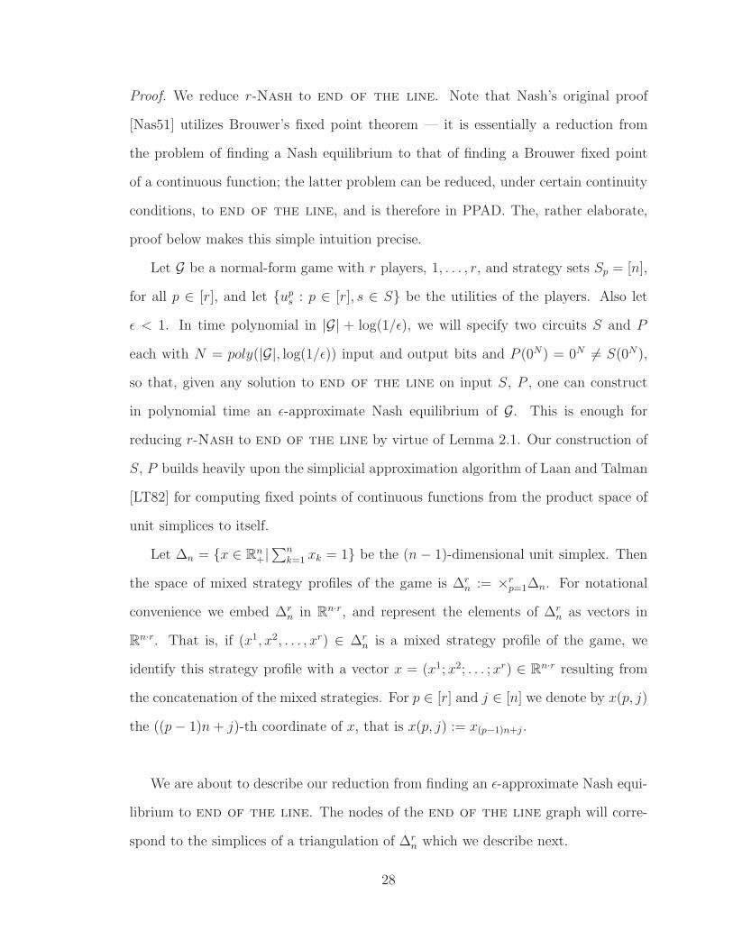
Proof. We reduce r-Nash to end of the line. Note that Nash’s original proof
[Nas51] utilizes Brouwer’s fixed point theorem — it is essentially a reduction from
the problem of finding a Nash equilibrium to that of finding a Brouwer fixed point
of a continuous function; the latter problem can be reduced, under certain continuity
conditions, to end of the line, and is therefore in PPAD. The, rather elaborate,
proof below makes this simple intuition precise.
Let G be a normal-form game with r players, 1, . . . , r, and strategy sets Sp = [n],
for all p ∈ [r], and let ups : p ∈ [r], s ∈ S be the utilities of the players. Also let
ǫ < 1. In time polynomial in |G| + log(1/ǫ), we will specify two circuits S and P
each with N = poly(|G|, log(1/ǫ)) input and output bits and P (0N) = 0N 6= S(0N),
so that, given any solution to end of the line on input S, P , one can construct
in polynomial time an ǫ-approximate Nash equilibrium of G. This is enough for
reducing r-Nash to end of the line by virtue of Lemma 2.1. Our construction of
S, P builds heavily upon the simplicial approximation algorithm of Laan and Talman
[LT82] for computing fixed points of continuous functions from the product space of
unit simplices to itself.
Let ∆n = x ∈ Rn+|∑n
k=1 xk = 1 be the (n − 1)-dimensional unit simplex. Then
the space of mixed strategy profiles of the game is ∆rn := ×r
p=1∆n. For notational
convenience we embed ∆rn in Rn·r, and represent the elements of ∆r
n as vectors in
Rn·r. That is, if (x1, x2, . . . , xr) ∈ ∆rn is a mixed strategy profile of the game, we
identify this strategy profile with a vector x = (x1; x2; . . . ; xr) ∈ Rn·r resulting from
the concatenation of the mixed strategies. For p ∈ [r] and j ∈ [n] we denote by x(p, j)
the ((p − 1)n + j)-th coordinate of x, that is x(p, j) := x(p−1)n+j .
We are about to describe our reduction from finding an ǫ-approximate Nash equi-
librium to end of the line. The nodes of the end of the line graph will corre-
spond to the simplices of a triangulation of ∆rn which we describe next.
28
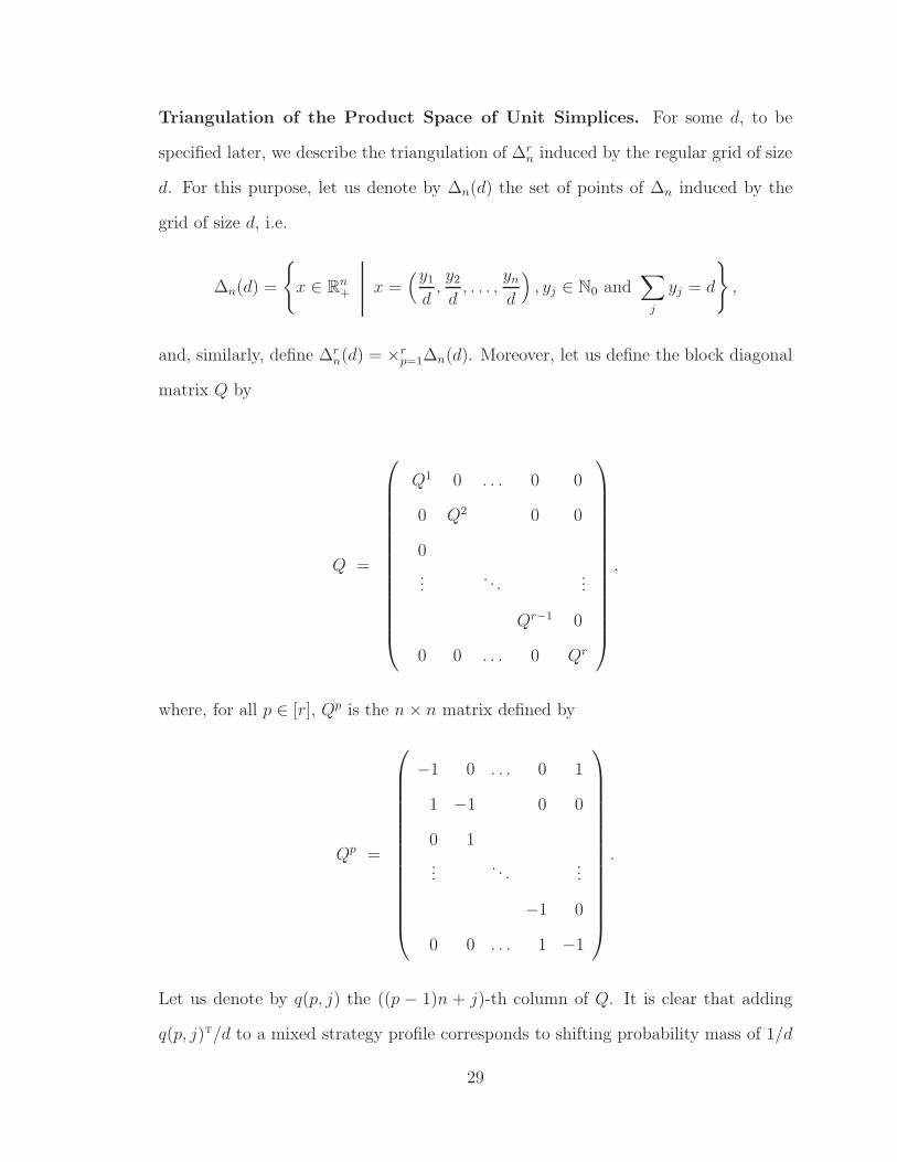
Triangulation of the Product Space of Unit Simplices. For some d, to be
specified later, we describe the triangulation of ∆rn induced by the regular grid of size
d. For this purpose, let us denote by ∆n(d) the set of points of ∆n induced by the
grid of size d, i.e.
∆n(d) =
x ∈ Rn
+ x =(y1
d,y2
d, . . . ,
yn
d
), yj ∈ N0 and
∑
j
yj = d
,
and, similarly, define ∆rn(d) = ×r
p=1∆n(d). Moreover, let us define the block diagonal
matrix Q by
Q =
Q1 0 . . . 0 0
0 Q2 0 0
0
.... . .
...
Qr−1 0
0 0 . . . 0 Qr
,
where, for all p ∈ [r], Qp is the n × n matrix defined by
Qp =
−1 0 . . . 0 1
1 −1 0 0
0 1
.... . .
...
−1 0
0 0 . . . 1 −1
.
Let us denote by q(p, j) the ((p − 1)n + j)-th column of Q. It is clear that adding
q(p, j)T/d to a mixed strategy profile corresponds to shifting probability mass of 1/d
29
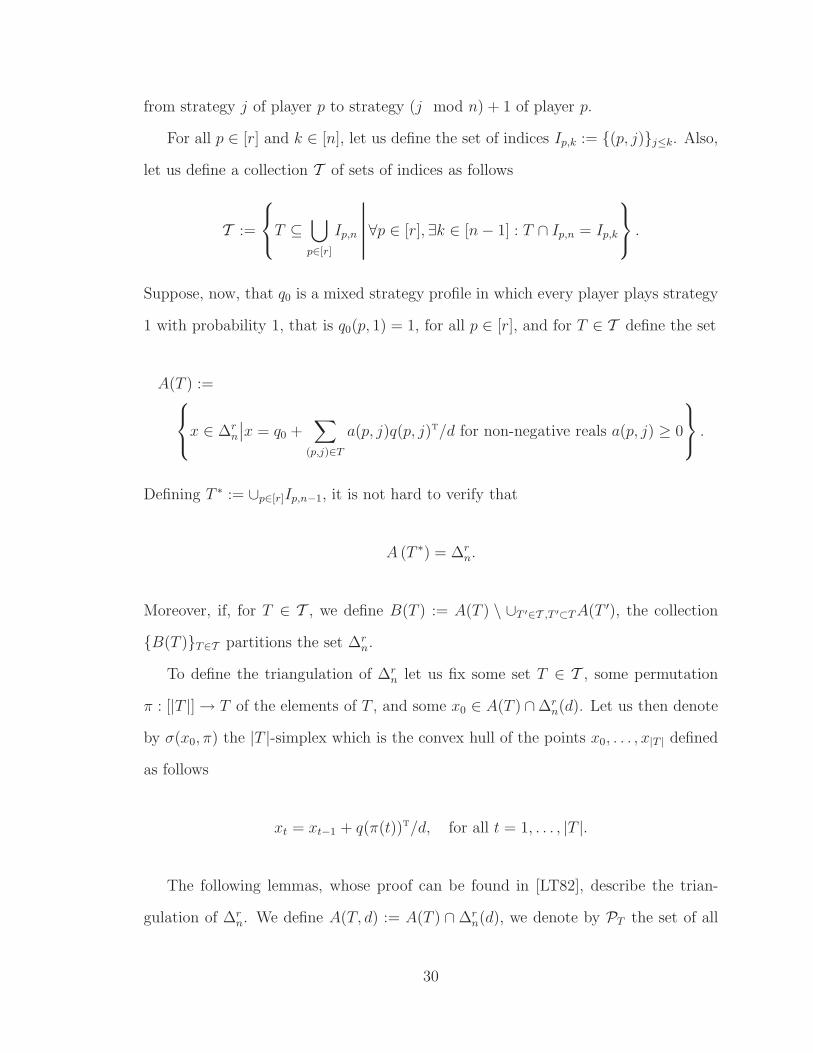
from strategy j of player p to strategy (j mod n) + 1 of player p.
For all p ∈ [r] and k ∈ [n], let us define the set of indices Ip,k := (p, j)j≤k. Also,
let us define a collection T of sets of indices as follows
T :=
T ⊆
⋃
p∈[r]
Ip,n ∀p ∈ [r], ∃k ∈ [n − 1] : T ∩ Ip,n = Ip,k
.
Suppose, now, that q0 is a mixed strategy profile in which every player plays strategy
1 with probability 1, that is q0(p, 1) = 1, for all p ∈ [r], and for T ∈ T define the set
A(T ) :=x ∈ ∆r
n
∣∣x = q0 +∑
(p,j)∈T
a(p, j)q(p, j)T/d for non-negative reals a(p, j) ≥ 0
.
Defining T ∗ := ∪p∈[r]Ip,n−1, it is not hard to verify that
A (T ∗) = ∆rn.
Moreover, if, for T ∈ T , we define B(T ) := A(T ) \ ∪T ′∈T ,T ′⊂T A(T ′), the collection
B(T )T∈T partitions the set ∆rn.
To define the triangulation of ∆rn let us fix some set T ∈ T , some permutation
π : [|T |] → T of the elements of T , and some x0 ∈ A(T ) ∩ ∆rn(d). Let us then denote
by σ(x0, π) the |T |-simplex which is the convex hull of the points x0, . . . , x|T | defined
as follows
xt = xt−1 + q(π(t))T/d, for all t = 1, . . . , |T |.
The following lemmas, whose proof can be found in [LT82], describe the trian-
gulation of ∆rn. We define A(T, d) := A(T ) ∩ ∆r
n(d), we denote by PT the set of all
30
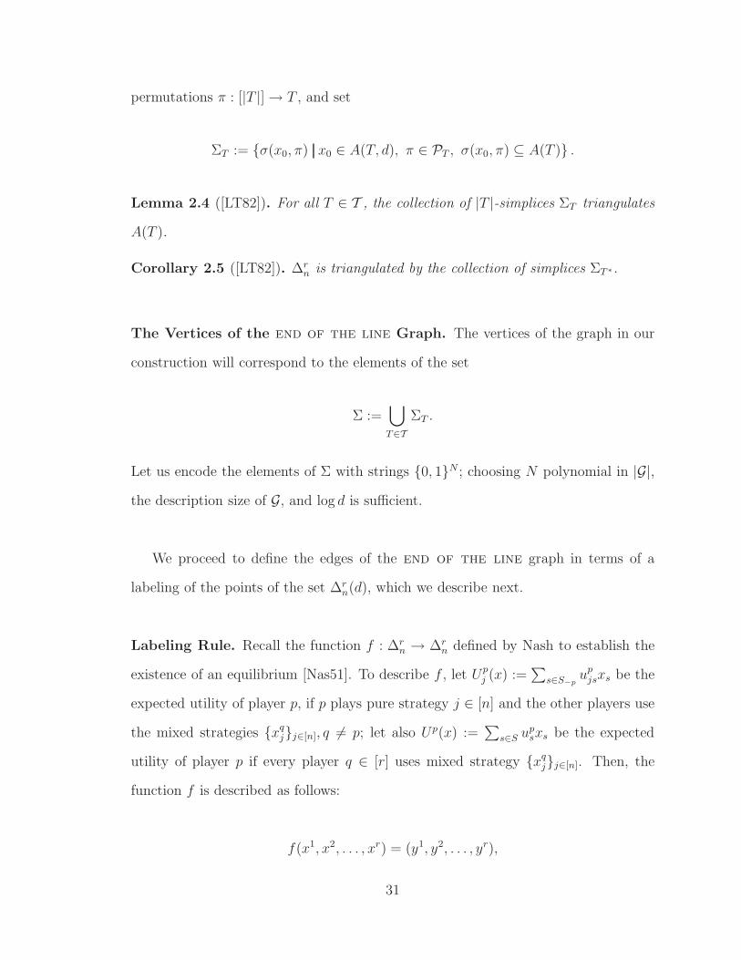
permutations π : [|T |] → T , and set
ΣT := σ(x0, π) x0 ∈ A(T, d), π ∈ PT , σ(x0, π) ⊆ A(T ) .
Lemma 2.4 ([LT82]). For all T ∈ T , the collection of |T |-simplices ΣT triangulates
A(T ).
Corollary 2.5 ([LT82]). ∆rn is triangulated by the collection of simplices ΣT ∗.
The Vertices of the end of the line Graph. The vertices of the graph in our
construction will correspond to the elements of the set
Σ :=⋃
T∈TΣT .
Let us encode the elements of Σ with strings 0, 1N ; choosing N polynomial in |G|,
the description size of G, and log d is sufficient.
We proceed to define the edges of the end of the line graph in terms of a
labeling of the points of the set ∆rn(d), which we describe next.
Labeling Rule. Recall the function f : ∆rn → ∆r
n defined by Nash to establish the
existence of an equilibrium [Nas51]. To describe f , let Upj (x) :=
∑s∈S−p
upjsxs be the
expected utility of player p, if p plays pure strategy j ∈ [n] and the other players use
the mixed strategies xqjj∈[n], q 6= p; let also Up(x) :=
∑s∈S up
sxs be the expected
utility of player p if every player q ∈ [r] uses mixed strategy xqjj∈[n]. Then, the
function f is described as follows:
f(x1, x2, . . . , xr) = (y1, y2, . . . , yr),
31
where, for each p ∈ [r], j ∈ [n],
ypj =
xpj + max (0, Up
j (x) − Up(x))
1 +∑
k∈[n] max (0, Upk (x) − Up(x))
.
It is not hard to see that f is continuous, and that f(x) can be computed in time
polynomial in the binary encoding size of x and G. Moreover, it can be verified that
any point x ∈ ∆rn such that f(x) = x is a Nash equilibrium [Nas51]. The following
lemma establishes that f is λ-Lipschitz for λ := [1 + 2Umaxrn(n + 1)], where Umax is
the maximum entry in the payoff tables of the game.
Lemma 2.6. For all x, x′ ∈ ∆rn ⊆ Rn·r such that ||x − x′||∞ ≤ δ,
||f(x) − f(x′)||∞ ≤ [1 + 2Umaxrn(n + 1)]δ.
Proof. We use the following bound shown in Section 3.6, Lemma 3.32.
Lemma 2.7. For any game G, for all p ≤ r, j ∈ Sp,
∣∣∣∣∣∣
∑
s∈S−p
upjsxs −
∑
s∈S−p
upjsx
′s
∣∣∣∣∣∣≤ max
s∈S−p
upjs∑
q 6=p
∑
i∈Sq
|xqi − x′q
i |.
It follows that for all p ∈ [r], j ∈ [n],
|Upj (x) − Up
j (x′)| ≤ Umaxrnδ
and |Up(x) − Up(x′)| ≤ Umaxrnδ.
Denoting Bpj (x) := max (0, Up
j (x) − Up(x)), for all p ∈ [r], j ∈ [n], the above bounds
32

imply that
|Bpj (x) − Bp
j (x′)| ≤ 2Umaxrnδ,∣∣∣∣∣∣
∑
k∈[n]
Bpk(x) −
∑
k∈[n]
Bpk(x′)
∣∣∣∣∣∣≤ 2Umaxrnδ · n.
Combining the above bounds we get that, for all p ∈ [r], j ∈ [n],
|ypj (x) − yp
j (x′)| ≤ |xpj − x′p
j | + |Bpj (x) − Bp
j (x′)| +
∣∣∣∣∣∣
∑
k∈[n]
Bpk(x) −
∑
k∈[n]
Bpk(x′)
∣∣∣∣∣∣
≤ δ + 2Umaxrnδ + 2Umaxrnδ · n
≤ [1 + 2Umaxrn(n + 1)]δ,
where we made use of the following lemma:
Lemma 2.8. For any x, x′, y, y′, z, z′ ≥ 0 such that x+y1+z
≤ 1,
∣∣∣∣x + y
1 + z− x′ + y′
1 + z′
∣∣∣∣ ≤ |x − x′| + |y − y′| + |z − z′|.
Proof.
∣∣∣∣x + y
1 + z− x′ + y′
1 + z′
∣∣∣∣ =
∣∣∣∣(x + y)(1 + z′) − (x′ + y′)(1 + z)
(1 + z)(1 + z′)
∣∣∣∣
=
∣∣∣∣(x + y)(1 + z′) − (x + y)(1 + z) − ((x′ − x) + (y′ − y))(1 + z)
(1 + z)(1 + z′)
∣∣∣∣
≤∣∣∣∣(x + y)(1 + z′) − (x + y)(1 + z)
(1 + z)(1 + z′)
∣∣∣∣ +
∣∣∣∣((x′ − x) + (y′ − y))(1 + z)
(1 + z)(1 + z′)
∣∣∣∣
≤∣∣∣∣(x + y)(z′ − z)
(1 + z)(1 + z′)
∣∣∣∣+ |x′ − x| + |y′ − y|
≤ x + y
1 + z|z′ − z| + |x′ − x| + |y′ − y| ≤ |z′ − z| + |x′ − x| + |y′ − y|.
33
We describe a labeling of the points of the set ∆rn(d) in terms of the function f .
The labels that we are going to use are the elements of the set L := ∪p∈[r]Ip,n. In
particular,
We assign to a point x ∈ ∆rn the label (p, j) iff (p, j) is the lexicographically least
index such that xpj > 0 and f(x)p
j − xpj ≤ f(x)q
k − xqk, for all q ∈ [r], k ∈ [n].
This labeling rule satisfies the following properties:
• Completeness: Every point x is assigned a label; hence, we can define a labeling
function ℓ : ∆rn → L.
• Properness: xpj = 0 implies ℓ(x) 6= (p, j).
• Efficiency: ℓ(x) is computable in time polynomial in the binary encoding size
of x and G.
A simplex σ ∈ Σ is called completely labeled if all its vertices have different labels;
a simplex σ ∈ Σ is called p-stopping if it is completely labeled and, moreover, for all
j ∈ [n], there exists a vertex of σ with label (p, j). Our labeling satisfies the following
important property.
Theorem 2.9 ([LT82]). Suppose a simplex σ ∈ Σ is p-stopping for some p ∈ [r].
Then all points x ∈ σ ⊆ Rn·r satisfy
||f(x) − x||∞ ≤ 1
d(λ + 1)n(n − 1).
Proof. It is not hard to verify that, for any simplex σ ∈ Σ and for all pairs of points
x, x′ ∈ σ,
||x − x′||∞ ≤ 1
d.
34
Suppose now that a simplex σ ∈ Σ is p-stopping, for some p ∈ [r], and that, for all
j ∈ [n], z(j) is the vertex of σ with label (p, j). Since, for any x,∑
i∈[n] xpi = 1 =
∑i∈[n] f(x)p
i , it follows from the labeling rule that
f(z(j))pj − z(j)p
j ≤ 0, ∀j ∈ [n].
Hence, for all x ∈ σ, j ∈ [n],
f(x)pj − xp
j ≤ f(z(j))pj − z(j)p
j + (λ + 1)1
d≤ (λ + 1)
1
d,
where we used the fact that the diameter of σ is 1d
(in the infinity norm) and the
function f is λ-Lipschitz. Hence, in the opposite direction, for all x ∈ σ, j ∈ [n], we
have
f(x)pj − xp
j = −∑
i∈[n]\j(f(x)p
i − xpi ) ≥ −(n − 1)(λ + 1)
1
d.
Now, by the definition of the labeling rule, we have, for all x ∈ σ, q ∈ [r], j ∈ [n],
f(x)qj − xq
j ≥ f(z(1))qj − z(1)q
j − (λ + 1)1
d
≥ f(z(1))p1 − z(1)p
1 − (λ + 1)1
d
≥ −(n − 1)(λ + 1)1
d− (λ + 1)
1
d= −n(λ + 1)
1
d,
whereas
f(x)qj − xq
j = −∑
i∈[n]\j(f(x)q
i − xqi )
≤ (n − 1)n(λ + 1)1
d.
35
Combining the above, it follows that, for all x ∈ σ,
||f(x) − x||∞ ≤ 1
d(λ + 1)n(n − 1).
The Approximation Guarantee. By virtue of Theorem 2.9, if we choose
d :=1
ǫ′[2 + 2Umaxrn(n + 1)]n(n − 1),
then a p-stopping simplex σ ∈ Σ, for any p ∈ [r], satisfies that, for all x ∈ σ,
||f(x) − x||∞ ≤ ǫ′,
which, by Lemma 2.10 below, implies that x is an approximate Nash equilibrium
achieving approximation
n√
ǫ′(1 + nUmax)(
1 +√
ǫ′(1 + nUmax))
maxUmax, 1.
Choosing
ǫ′ :=1
1 + nUmax
(ǫ
2n maxUmax, 1
)2
,
we have that x is an ǫ-approximate Nash equilibrium.
Lemma 2.10. If a vector x = (x1; x2; . . . ; xr) ∈ Rn·r satisfies
||f(x) − x||∞ ≤ ǫ′,
then x is a n√
ǫ′(1 + nUmax)(
1 +√
ǫ′(1 + nUmax))
maxUmax, 1-approximate Nash
36
equilibrium.
Proof. Let us fix some player p ∈ [r], and assume, without loss of generality, that
Up1 (x) ≥ Up
2 (x) ≥ . . . ≥ Upk (x) ≥ Up(x) ≥ Up
k+1(x) ≥ . . . ≥ Upn(x).
For all j ∈ [n], observe that |f(x)pj − xp
j | ≤ ǫ′ implies
xpj
∑
i∈[n]
Bpi (x) ≤ Bp
j (x) + ǫ′
1 +
∑
i∈[n]
Bpi (x)
.
Setting ǫ′′ := ǫ′(1 + nUmax), the above inequality implies
xpj
∑
i∈[n]
Bpi (x) ≤ Bp
j (x) + ǫ′′. (2.3)
Let us define t := xpk+1 + xp
k+2 + . . . + xpn, and let us distinguish the following cases
• If t ≥√
ǫ′′
Umax, then summing Equation (2.3) for j = k + 1, . . . , n implies
t∑
i∈[n]
Bpi (x) ≤ (n − k)ǫ′′,
which gives
Bp1 ≤
∑
i∈[n]
Bpi (x) ≤ n
√ǫ′′Umax. (2.4)
• If t ≤√
ǫ′′
Umax, then multiplying Equation (2.3) by xp
j and summing over j =
1, . . . , n gives
∑
j∈[n]
(xpj )2∑
i∈[n]
Bpi (x) ≤
∑
j∈[n]
xpjB
pj (x) + ǫ′′. (2.5)
37
Now observe that for any setting of the probabilities xpj , j ∈ [n], it holds that
∑
j∈[n]
(xpj )2 ≥ 1
n. (2.6)
Moreover, observe that, since Up(x) =∑
j∈[n] xpjU
pj (x), it follows that
∑
j∈[n]
xpj (Up
j (x) − Up(x)) = 0,
which implies that
∑
j∈[n]
xpjB
pj (x) +
∑
j≥k+1
xpj (Up
j (x) − Up(x)) = 0.
Plugging this into (2.5) implies
∑
j∈[n]
(xpj )2∑
i∈[n]
Bpi (x) ≤
∑
j≥k+1
xpj (Up(x) − Up
j (x)) + ǫ′′.
Further, using (2.6) gives
1
n
∑
i∈[n]
Bpi (x) ≤
∑
j≥k+1
xpj (Up(x) − Up
j (x)) + ǫ′′,
which implies∑
i∈[n]
Bpi (x) ≤ n(tUmax + ǫ′′).
The last inequality then implies
Bp1(x) ≤ n(
√ǫ′′ + ǫ′′). (2.7)
38
Combining (2.4) and (2.7), we have the following uniform bound
Bp1(x) ≤ n(
√ǫ′′ + ǫ′′) maxUmax, 1 =: ǫ′′′. (2.8)
Since Bp1(x) = Up
1 (x) − U(x), it follows that player p cannot improve her payoff by
more that ǫ′′′ by changing her strategy. This is true for every player, hence x is a
ǫ′′′-approximate Nash equilibrium.
The Edges of the end of the line Graph. Laan and Talman [LT82] describe a
pivoting algorithm which operates on the set Σ, by specifying the following:
• a simplex σ0 ∈ Σ, which is the starting simplex; σ0 contains the point q0 and is
uniquely determined by the labeling rule;
• a partial one-to-one function h : Σ → Σ, mapping a simplex to a neighboring
simplex, which defines a pivoting rule; h has the following properties: 1
– σ0 has no pre-image;
– any simplex σ ∈ Σ that has no image is a p-stopping simplex for some
p; and, any simplex σ ∈ Σ \ σ0 that has no pre-image is a p-stopping
simplex for some p;
– both h(σ) and h−1(σ) are computable in time polynomial in the binary
encoding size of σ, that is N , and G —given that the labeling function ℓ
is efficiently computable;
The algorithm of Laan and Talman starts off with the simplex σ0 and employs the
pivoting rule h until a simplex σ with no image is encountered. By the properties
1More precisely, the pivoting rule h of Laan and Talman is defined on a subset Σ′ of Σ. For ourpurposes, let us extend their pivoting rule h to the set Σ by setting h(σ) = σ for all σ ∈ Σ \ Σ′.
39
of h, σ must be p-stopping for some p ∈ [r] and, by the discussion above, any point
x ∈ σ is an ǫ-approximate Nash equilibrium.
In our construction, the edges of the end of the line graph are defined in terms
of the function h: if h(σ) = σ′, then there is a directed edge from σ to σ′. Moreover,
the string 0N is identified with the simplex σ0. Any solution to the end of the
line problem thus defined corresponds by the above discussion to a simplex σ such
that any point x ∈ σ is an ǫ-approximate Nash equilibrium of G. This concludes the
construction.
2.4 Brouwer: a PPAD-Complete Fixed Point Com-
putation Problem
To show that Nash is PPAD-hard, we use a problem we call Brouwer, which is a
discrete and simplified version of the search problem associated with Brouwer’s fixed
point theorem. We are given a continuous function φ from the 3-dimensional unit
cube to itself, defined in terms of its values at the centers of 23n cubelets with side
2−n, for some n ≥ 0. 2 At the center cijk of the cubelet Kijk defined as
Kijk = (x, y, z) : i · 2−n ≤ x ≤ (i + 1) · 2−n,
j · 2−n ≤ y ≤ (j + 1) · 2−n,
k · 2−n ≤ z ≤ (k + 1) · 2−n,
where i, j, k are integers in 0, 1, . . . , 2n − 1, the value of φ is φ(cijk) = cijk + δijk,
where δijk is one of the following four vectors (also referred to as colors):
2The value of the function near the boundaries of the cubelets could be determined by interpo-lation —there are many simple ways to do this, and the precise method is of no importance to ourdiscussion.
40
• δ1 = (α, 0, 0)
• δ2 = (0, α, 0)
• δ3 = (0, 0, α)
• δ0 = (−α,−α,−α)
Here α > 0 is much smaller than the cubelet side, say 2−2n.
Thus, to compute φ at the center of the cubelet Kijk we only need to know which
of the four displacements to add. This is computed by a circuit C (which is the only
input to the problem) with 3n input bits and 2 output bits; C(i, j, k) is the index r
such that, if c is the center of cubelet Kijk, φ(c) = c+δr. C is such that C(0, j, k) = 1,
C(i, 0, k) = 2, C(i, j, 0) = 3, and C(2n − 1, j, k) = C(i, 2n − 1, k) = C(i, j, 2n − 1) = 0
(with conflicts resolved arbitrarily), so that the function φ maps the boundary to
the interior of the cube. A vertex of a cubelet is called panchromatic if among the
cubelets adjacent to it there are four that have all four displacements δ0, δ1, δ2, δ3.
Sperner’s Lemma guarantees that, for any circuit C satisfying the above properties,
a panchromatic vertex exists, see, e.g., [Pap94b]. An alternative proof of this fact
follows as a consequence of Theorem 2.11 below.
Brouwer is thus the following total problem: Given a circuit C as described
above, find a panchromatic vertex. The relationship with Brouwer fixed points is
that fixed points of φ only ever occur in the vicinity of a panchromatic vertex. We
next show:
Theorem 2.11. Brouwer is PPAD-complete.
Proof. That Brouwer is in PPAD follows from Theorem 4.1, which is a reduction
from Brouwer to r-Nash, which has been shown to be in PPAD in Theorem 2.3.
To show hardness, we shall reduce end of the line to Brouwer. Given circuits
S and P with n inputs and outputs, as prescribed in that problem, we shall construct
41
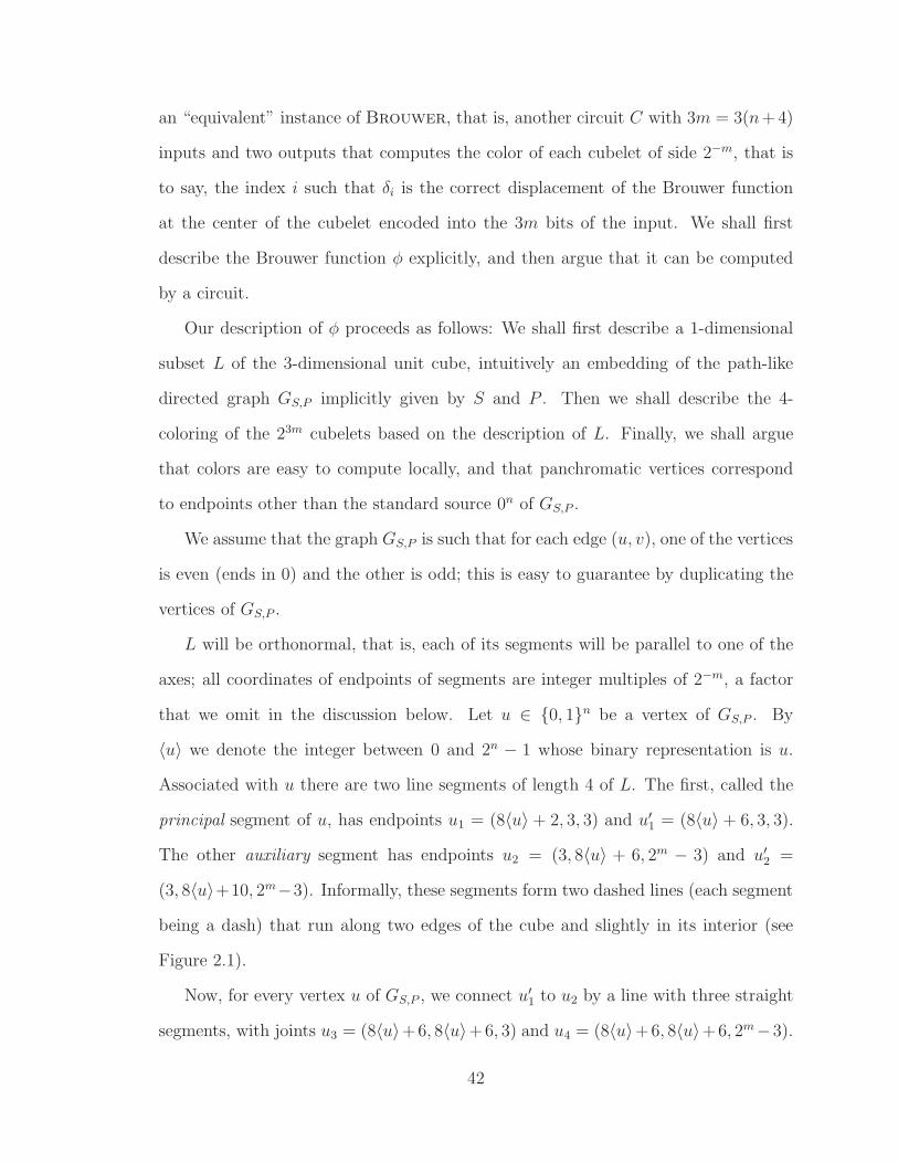
an “equivalent” instance of Brouwer, that is, another circuit C with 3m = 3(n+ 4)
inputs and two outputs that computes the color of each cubelet of side 2−m, that is
to say, the index i such that δi is the correct displacement of the Brouwer function
at the center of the cubelet encoded into the 3m bits of the input. We shall first
describe the Brouwer function φ explicitly, and then argue that it can be computed
by a circuit.
Our description of φ proceeds as follows: We shall first describe a 1-dimensional
subset L of the 3-dimensional unit cube, intuitively an embedding of the path-like
directed graph GS,P implicitly given by S and P . Then we shall describe the 4-
coloring of the 23m cubelets based on the description of L. Finally, we shall argue
that colors are easy to compute locally, and that panchromatic vertices correspond
to endpoints other than the standard source 0n of GS,P .
We assume that the graph GS,P is such that for each edge (u, v), one of the vertices
is even (ends in 0) and the other is odd; this is easy to guarantee by duplicating the
vertices of GS,P .
L will be orthonormal, that is, each of its segments will be parallel to one of the
axes; all coordinates of endpoints of segments are integer multiples of 2−m, a factor
that we omit in the discussion below. Let u ∈ 0, 1n be a vertex of GS,P . By
〈u〉 we denote the integer between 0 and 2n − 1 whose binary representation is u.
Associated with u there are two line segments of length 4 of L. The first, called the
principal segment of u, has endpoints u1 = (8〈u〉 + 2, 3, 3) and u′1 = (8〈u〉 + 6, 3, 3).
The other auxiliary segment has endpoints u2 = (3, 8〈u〉 + 6, 2m − 3) and u′2 =
(3, 8〈u〉+10, 2m−3). Informally, these segments form two dashed lines (each segment
being a dash) that run along two edges of the cube and slightly in its interior (see
Figure 2.1).
Now, for every vertex u of GS,P , we connect u′1 to u2 by a line with three straight
segments, with joints u3 = (8〈u〉+ 6, 8〈u〉+ 6, 3) and u4 = (8〈u〉+ 6, 8〈u〉+ 6, 2m−3).
42

u′
2
u1u3
v′1
y
v1
u′
1
u6
u4
u5
u2
z
x
Figure 2.1: The orthonormal path connecting vertices (u,v); the arrows indicate theorientation of colors surrounding the path.
Finally, if there is an edge (u, v) in GS,P , we connect u′2 to v1 by a jointed line with
breakpoints u5 = (8〈v〉 + 2, 8〈u〉 + 10, 2m − 3) and u6 = (8〈v〉 + 2, 8〈u〉 + 10, 3).
This completes the description of the line L if we do the following perturbation:
exceptionally, the principal segment of u = 0n has endpoints 01 = (2, 2, 2) and 0′1 =
(6, 2, 2) and the corresponding joint is 03 = (6, 6, 2).
It is easy to see that L traverses the interior of the cube without ever “nearly
crossing itself”; that is, two points p, p′ of L are closer than 3 · 2−m in Euclidean
distance only if they are connected by a part of L that has length 8 ·2−m or less. (This
is important in order for the coloring described below of the cubelets surrounding L
to be well-defined.) To check this, just notice that segments of different types (e.g.,
43
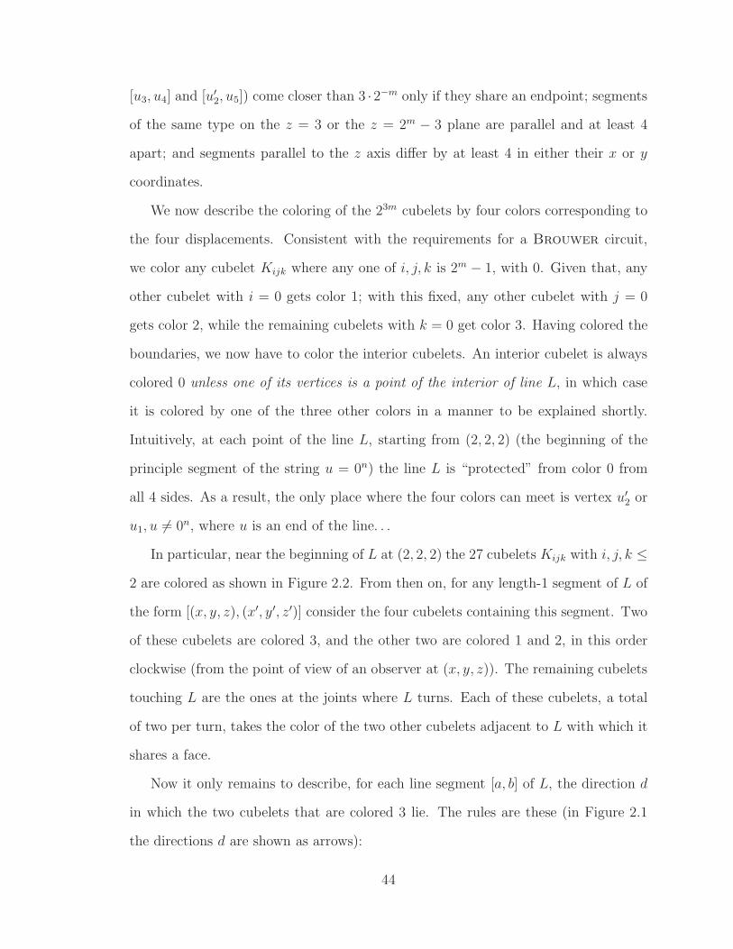
[u3, u4] and [u′2, u5]) come closer than 3 ·2−m only if they share an endpoint; segments
of the same type on the z = 3 or the z = 2m − 3 plane are parallel and at least 4
apart; and segments parallel to the z axis differ by at least 4 in either their x or y
coordinates.
We now describe the coloring of the 23m cubelets by four colors corresponding to
the four displacements. Consistent with the requirements for a Brouwer circuit,
we color any cubelet Kijk where any one of i, j, k is 2m − 1, with 0. Given that, any
other cubelet with i = 0 gets color 1; with this fixed, any other cubelet with j = 0
gets color 2, while the remaining cubelets with k = 0 get color 3. Having colored the
boundaries, we now have to color the interior cubelets. An interior cubelet is always
colored 0 unless one of its vertices is a point of the interior of line L, in which case
it is colored by one of the three other colors in a manner to be explained shortly.
Intuitively, at each point of the line L, starting from (2, 2, 2) (the beginning of the
principle segment of the string u = 0n) the line L is “protected” from color 0 from
all 4 sides. As a result, the only place where the four colors can meet is vertex u′2 or
u1, u 6= 0n, where u is an end of the line. . .
In particular, near the beginning of L at (2, 2, 2) the 27 cubelets Kijk with i, j, k ≤
2 are colored as shown in Figure 2.2. From then on, for any length-1 segment of L of
the form [(x, y, z), (x′, y′, z′)] consider the four cubelets containing this segment. Two
of these cubelets are colored 3, and the other two are colored 1 and 2, in this order
clockwise (from the point of view of an observer at (x, y, z)). The remaining cubelets
touching L are the ones at the joints where L turns. Each of these cubelets, a total
of two per turn, takes the color of the two other cubelets adjacent to L with which it
shares a face.
Now it only remains to describe, for each line segment [a, b] of L, the direction d
in which the two cubelets that are colored 3 lie. The rules are these (in Figure 2.1
the directions d are shown as arrows):
44

z y
x
Z=2
Z=1
Z=0
1 1 1
22
1
22
1
11
1
23
3
23
3
11
1
23
3
23
3
Beginning of L
Figure 2.2: The 27 cubelets around the beginning of line L.
• If [a, b] = [u1, u′1] then d = (0, 0,−1) if u is even and d = (0, 0, 1) if u is odd.
• If [a, b] = [u′1, u3] then d = (0, 0,−1) if u is even and d = (0, 0, 1) if u is odd.
• If [a, b] = [u3, u4] then d = (0, 1, 0) if u is even and d = (0,−1, 0) if u is odd.
• If [a, b] = [u4, u2] then d = (0, 1, 0) if u is even and d = (0,−1, 0) if u is odd.
• If [a, b] = [u2, u′2] then d = (1, 0, 0) if u is even and d = (−1, 0, 0) if u is odd.
• If [a, b] = [u′2, u5] then d = (0,−1, 0) if u is even and d = (0, 1, 0) if u is odd.
• If [a, b] = [u5, u6] then d = (0,−1, 0) if u is even and d = (0, 1, 0) if u is odd.
• If [a, b] = [u6, v1] then d = (0, 0, 1) if u is even and d = (0, 0,−1) if u is odd.
This completes the description of the construction. Notice that, for this to work,
we need our assumption that edges in GS,P go between odd and even vertices. Regard-
45
ing the alternating orientation of colored cubelets around L, note that we could not
simply introduce “twists” to make them always point in (say) direction d = (0, 0,−1)
for all [u1, u′1]. That would create a panchromatic vertex at the location of a twist.
The result now follows from the following two claims:
1. A point in the cube is panchromatic in the described coloring if and only if it is
(a) an endpoint u′2 of a sink vertex u of GS,P , or
(b) an endpoint u1 of a source vertex u 6= 0n of GS,P
2. A circuit C can be constructed in time polynomial in |S|+ |P |, which computes,
for each triple of binary integers i, j, k < 2m, the color of cubelet Kijk.
Regarding the first claim, the endpoint u′2 of a sink vertex u, or the endpoint u1
of a source vertex u other than 0n, will be a point where L meets color 0, hence a
panchromatic vertex. There is no alternative way that L can meet color 0 and no
other way a panchromatic vertex can occur.
Regarding the second claim, circuit C is doing the following. C(0, j, k) = 1, for
j, k < 2m − 1, C(i, 0, k) = 2 for i > 0, i, k < 2m − 1, C(i, j, 0) = 3 for i, j > 0,
i, j < 2m − 1. Then by default, C(i, j, k) = 0. However the following tests yield
alternative values for C(i, j, k), for cubelets adjacent to L. LSB(x) denotes the least
significant bit of x, equal to 1 if x is odd, 0 if x is even, and undefined if x is not an
integer. For example, a [u′1, u3], u 6= 0n segment is given by (letting x = 〈u〉):
1. If k = 2 and i = 8x + 5 and LSB(x) = 1 and j ∈ 3, . . . , 8x + 6 then
C(i, j, k) = 2.
2. If k = 2 and i = 8x + 6 and LSB(x) = 1 and j ∈ 2, . . . , 8x + 6 then
C(i, j, k) = 1.
46
3. If k = 3 and (i = 8x+ 5 or i = 8x+ 6) and LSB(x) = 1 and j ∈ 2, . . . , 8x+ 5
then C(i, j, k) = 3.
4. If k = 2 and (i = 8x+ 5 or i = 8x+ 6) and LSB(x) = 0 and j ∈ 2, . . . , 8x+ 6
then C(i, j, k) = 3.
5. If k = 3 and i = 8x + 5 and LSB(x) = 0 and j ∈ 3, . . . , 8x + 5 then
C(i, j, k) = 1.
6. If k = 3 and i = 8x + 6 and LSB(x) = 0 and j ∈ 2, . . . , 8x + 5 then
C(i, j, k) = 2.
A [u′2, u5] segment uses the circuits P and S, and, in the case LSB(x) = 1, x = 〈u〉,
is given by:
1. If (k = 2m − 3 or k = 2m − 4) and j = 8x + 10 and S(x) = x′ and P (x′) = x
and i ∈ 2, . . . , 8x′ + 2 then C(i, j, k) = 3.
2. If k = 2m − 3 and and j = 8x + 9 and S(x) = x′ and P (x′) = x and i ∈
3, . . . , 8x′ + 2 then C(i, j, k) = 1.
3. If k = 2m−4 and j = 8x+9 and S(x) = x′ and P (x′) = x and i ∈ 3, . . . , 8x′+1
then C(i, j, k) = 2.
The other segments are done in a similar way, and so the second claim follows. This
completes the proof of hardness.
47
2.5 Related Work on Computing Nash Equilibria
and Other Fixed Points
Over the past fifty years, a wealth of studies in the Economics, Optimization, and
Computer Science literature address the problem of computing Nash equilibria. A
celebrated algorithm for the case of two-player games is the Lemke-Howson algo-
rithm [LH64], which is remarkably similar to the simplex method, and appears to
be very efficient in practice. Rosenmuller [Ros71] and Wilson [Wil71] generalize the
Lemke-Howson algorithm to the multi-player case; however, this generalization re-
sults in significant loss in efficiency. More practical algorithms for the multi-player
case are based on general purpose methods for approximating Brouwer fixed points,
most notably on algorithms that walk on simplicial subdivisions of the space where
the equilibria lie, so-called simplicial algorithms [Sca67, GLL73, LT79, LT82, Eav72].
Despite much research on the subject, none of the existing methods for comput-
ing Nash equilibria are known to run in polynomial time, and there are negative
results [HPV89], even for the Lemke-Howson algorithm [SS04].
Lipton and Markakis [LM04] study the algebraic properties of Nash equilibria and
point out that standard quantifier elimination algorithms can be used to solve them,
but these do not run in polynomial time in general. Papadimitriou and Roughgarden
[PR05] show that, in the case of symmetric games, quantifier elimination results in
polynomial-time algorithms for a broad range of parameters. Lipton, Markakis and
Mehta [LMM03] show that, if we only require an ǫ-approximate Nash equilibrium,
then a subexponential algorithm is possible. If the Nash equilibria sought are required
to have any special properties, for example optimize total utility, the problem typically
becomes NP-complete [GZ89, CS03].
In addition to our results in Chapter 3, other researchers have explored reductions
between alternative types of games (see, e.g., [Bub79, AKV05, CSVY06, SV06]). In
48
particular, the reductions by Bubelis [Bub79] in the 1970s comprise a remarkable early
precursor of our work; it is astonishing that these important results had not been
pursued for three decades. Bubelis established that the Nash equilibrium problem
for 3 players captures the computational complexity of the same problem with any
number of players. In Chapter 3, we show the same result in an indirect way, via
the Nash equilibrium problem for graphical games — a connection that is crucial
for our PPAD-completeness reduction. Bubelis also demonstrated in [Bub79] that
any algebraic number can be the basis of a Nash equilibrium, something that follows
easily from our results (see Theorem 4.14).
Etessami and Yannakakis study in [EY07] the problem of computing a Nash equi-
librium exactly (a problem that is well-motivated in the context of stochastic games)
and provide an interesting characterization of its complexity (considerably higher
than PPAD), along with that of several other problems. In Section 4.3, we mention
certain interesting results at the interface of their approach with ours.
Finally, Adler and Verma show that several important sub-classes of the Linear
Complementarity Problem (LCP) belong to the class PPAD [AV07]. Using our results
from Chapter 4, they also establish that some of these classes, e.g., the LCP for strictly
co-positive and for strictly semi-monotone matrices, are PPAD-complete.
49
Chapter 3
Reductions Among Equilibrium
Problems
In Chapter 4, we show that r-Nash is PPAD-hard by reducing Brouwer to it.
Rather than r-Nash, it will be more convenient to first reduce Brouwer to d-
graphical Nash, the problem of computing a Nash equilibrium in graphical games
of degree d, defined in Section 2.2. Therefore, we need to show that the latter reduces
to r-Nash. This will be the purpose of the present chapter; in fact, we will establish
something stronger, namely that
Theorem 3.1. For every fixed d, r ≥ 3,
• Every r-player normal-form game and every graphical game of degree d can
be mapped in polynomial time to (a) a 3-player normal-form game and (b) a
graphical game with degree 3 and 2 strategies per player, such that there is a
polynomial-time computable surjective mapping from the set of Nash equilibria
of the latter to the set of Nash equilibria of the former.
• There are polynomial-time reductions from r-Nash and d-graphical Nash to
both 3-Nash and 3-graphical Nash.
50
Note that the first part of the theorem establishes mappings of exact equilibrium
points among different games, whereas the second asserts that computing approximate
equilibrium points in all these games is polynomial-time equivalent. The proof, which
is quite involved, is presented in the following sections. In Section 3.1, we present
some useful ideas that enable the reductions described in Theorem 3.1, as well as
prepare the necessary machinery for the reduction from Brouwer to d-graphical
Nash in Section 4.1. Sections 3.2 through 3.6 provide the proof of the theorem. We
note that a mapping from r-player games to 3-player games was already known by
Bubelis [Bub79].
In Section 3.7, we establish the computational equivalence of the two notions of
approximation discussed in Section 2.1. In particular, we give a polynomial-time
reduction from the problem of computing an approximately well supported Nash
equilibrium to the problem of computing an approximate Nash equilibrium. The
opposite reduction is trivial, as discussed in Section 2.1.
3.1 Preliminaries: Game Gadgets
We describe the building blocks of our constructions. As we have observed earlier, if a
player v has two pure strategies, say 0 and 1, then every mixed strategy of that player
corresponds to a real number p[v] ∈ [0, 1] which is precisely the probability that the
player plays strategy 1. Identifying players with these numbers, we are interested in
constructing games that perform simple arithmetical operations on mixed strategies;
for example, we are interested in constructing a game with two “input” players v1
and v2 and another “output” player v3 so that in any Nash equilibrium the latter
plays the sum of the former, i.e., p[v3] = minp[v1] + p[v2], 1. Such constructions
are considered below.
51
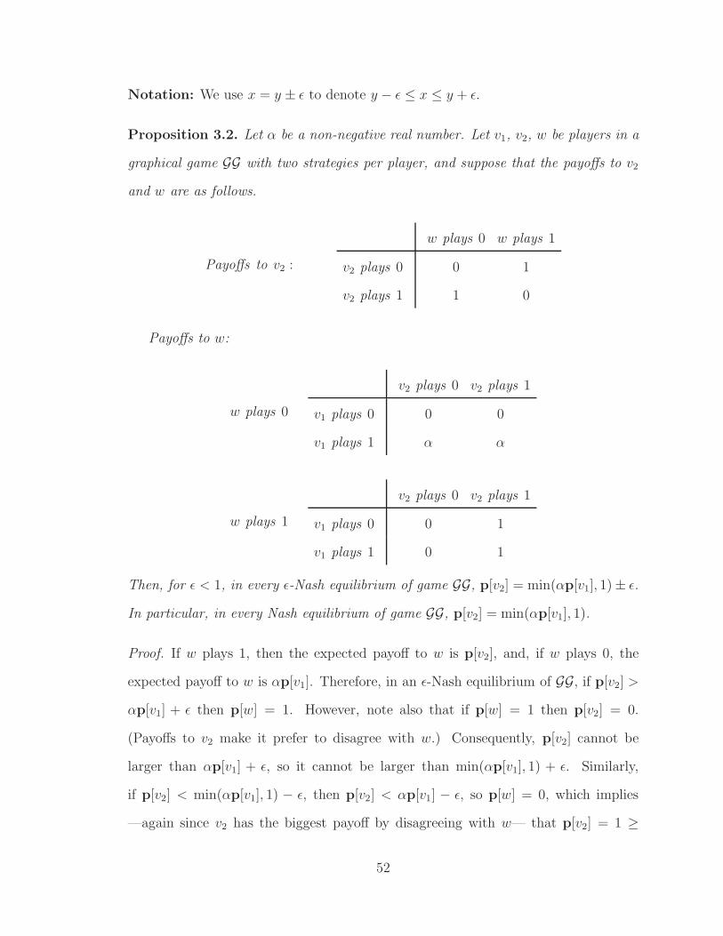
Notation: We use x = y ± ǫ to denote y − ǫ ≤ x ≤ y + ǫ.
Proposition 3.2. Let α be a non-negative real number. Let v1, v2, w be players in a
graphical game GG with two strategies per player, and suppose that the payoffs to v2
and w are as follows.
Payoffs to v2 :
w plays 0 w plays 1
v2 plays 0 0 1
v2 plays 1 1 0
Payoffs to w:
w plays 0
v2 plays 0 v2 plays 1
v1 plays 0 0 0
v1 plays 1 α α
w plays 1
v2 plays 0 v2 plays 1
v1 plays 0 0 1
v1 plays 1 0 1
Then, for ǫ < 1, in every ǫ-Nash equilibrium of game GG, p[v2] = min(αp[v1], 1) ± ǫ.
In particular, in every Nash equilibrium of game GG, p[v2] = min(αp[v1], 1).
Proof. If w plays 1, then the expected payoff to w is p[v2], and, if w plays 0, the
expected payoff to w is αp[v1]. Therefore, in an ǫ-Nash equilibrium of GG, if p[v2] >
αp[v1] + ǫ then p[w] = 1. However, note also that if p[w] = 1 then p[v2] = 0.
(Payoffs to v2 make it prefer to disagree with w.) Consequently, p[v2] cannot be
larger than αp[v1] + ǫ, so it cannot be larger than min(αp[v1], 1) + ǫ. Similarly,
if p[v2] < min(αp[v1], 1) − ǫ, then p[v2] < αp[v1] − ǫ, so p[w] = 0, which implies
—again since v2 has the biggest payoff by disagreeing with w— that p[v2] = 1 ≥
52

w
v2
v1
Figure 3.1: G×α, G=
w
v1
Figure 3.2: Gα
v3
w
v2v1
Figure 3.3: G+,G∗,G−
1 − ǫ, a contradiction to p[v2] < min(αp[v1], 1) − ǫ. Hence p[v2] cannot be less than
min(αp[v1], 1) − ǫ.
We will denote by G×α the (directed) graphical game shown in Figure 3.1, where
the payoffs to players v2 and w are specified as in Proposition 3.2 and the payoff of
player v1 is completely unconstrained: v1 could have any dependence on other players
of a larger graphical game GG that contains G×α or even depend on the strategies of
v2 and w; as long as the payoffs of v2 and w are specified as above the conclusion
of the proposition will be true. Note in particular that using the above construction
with α = 1, v2 becomes a “copy” of v1; we denote the corresponding graphical game
by G=. These graphical games will be used as building blocks in our constructions;
the way to incorporate them into some larger graphical game is to make player v1
depend (incoming edges) on other players of the game and make v2 affect (outgoing
edges) other players of the game. For example, we can make a sequence of copies
of any vertex, which form a path in the graph. The copies will then alternate with
distinct w vertices.
Proposition 3.3. Let α, β, γ be non-negative real numbers. Let v1, v2, v3, w be
players in a graphical game GG with two strategies per player, and suppose that the
53

payoffs to v3 and w are as follows.
Payoffs to v3 :
w plays 0 w plays 1
v3 plays 0 0 1
v3 plays 1 1 0
Payoffs to w:
w plays 0
v2 plays 0 v2 plays 1
v1 plays 0 0 β
v1 plays 1 α α + β + γ
w plays 1 v3 plays 0 0
v3 plays 1 1
Then, for ǫ < 1, in any ǫ-Nash equilibrium of GG, p[v3] = min(αp[v1] + βp[v2] +
γp[v1]p[v2], 1)±ǫ. In particular, in every Nash equilibrium of GG, p[v3] = min(αp[v1]+
βp[v2] + γp[v1]p[v2], 1).
Proof. If w plays 1, then the expected payoff to w is p[v3], and if w plays 0 then
the expected payoff to w is αp[v1] + βp[v2] + γp[v1]p[v2]. Therefore, in an ǫ-Nash
equilibrium of GG, if p[v3] > αp[v1]+βp[v2]+γp[v1]p[v2]+ǫ then p[w] = 1. However,
note from the payoffs to v3 that if p[w] = 1 then p[v3] = 0. Consequently, p[v3]
cannot be strictly larger than αp[v1] + βp[v2] + γp[v1]p[v2] + ǫ. Similarly, if p[v3] <
min(αp[v1]+βp[v2]+γp[v1]p[v2], 1)−ǫ, then p[v3] < αp[v1]+βp[v2]+γp[v1]p[v2]−ǫ
and, due to the payoffs to w, p[w] = 0. This in turn implies —since v3 has the
biggest payoff by disagreeing with w— that p[v3] = 1 ≥ 1 − ǫ, a contradiction to
p[v3] < min(αp[v1] + βp[v2] + γp[v1]p[v2], 1) − ǫ. Hence p[v3] cannot be less than
min(αp[v1] + βp[v2] + γp[v1]p[v2], 1) − ǫ.
54
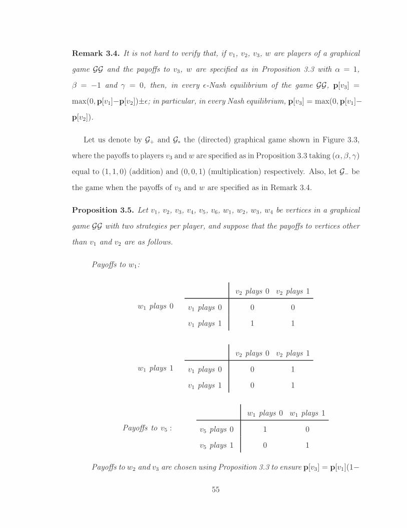
Remark 3.4. It is not hard to verify that, if v1, v2, v3, w are players of a graphical
game GG and the payoffs to v3, w are specified as in Proposition 3.3 with α = 1,
β = −1 and γ = 0, then, in every ǫ-Nash equilibrium of the game GG, p[v3] =
max(0,p[v1]−p[v2])±ǫ; in particular, in every Nash equilibrium, p[v3] = max(0,p[v1]−
p[v2]).
Let us denote by G+ and G∗ the (directed) graphical game shown in Figure 3.3,
where the payoffs to players v3 and w are specified as in Proposition 3.3 taking (α, β, γ)
equal to (1, 1, 0) (addition) and (0, 0, 1) (multiplication) respectively. Also, let G− be
the game when the payoffs of v3 and w are specified as in Remark 3.4.
Proposition 3.5. Let v1, v2, v3, v4, v5, v6, w1, w2, w3, w4 be vertices in a graphical
game GG with two strategies per player, and suppose that the payoffs to vertices other
than v1 and v2 are as follows.
Payoffs to w1:
w1 plays 0
v2 plays 0 v2 plays 1
v1 plays 0 0 0
v1 plays 1 1 1
w1 plays 1
v2 plays 0 v2 plays 1
v1 plays 0 0 1
v1 plays 1 0 1
Payoffs to v5 :
w1 plays 0 w1 plays 1
v5 plays 0 1 0
v5 plays 1 0 1
Payoffs to w2 and v3 are chosen using Proposition 3.3 to ensure p[v3] = p[v1](1−
55
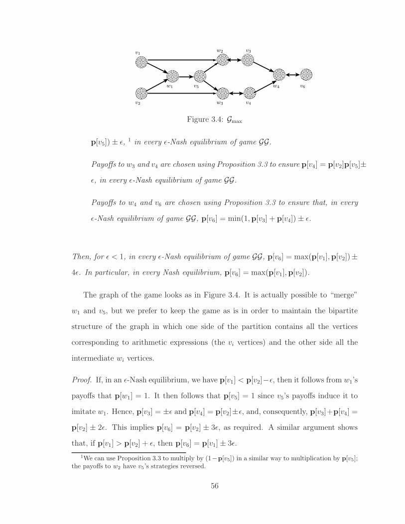
v6
v1
v2
w1 v5
w3
w2 v3
v4
w4
Figure 3.4: Gmax
p[v5]) ± ǫ, 1 in every ǫ-Nash equilibrium of game GG.
Payoffs to w3 and v4 are chosen using Proposition 3.3 to ensure p[v4] = p[v2]p[v5]±
ǫ, in every ǫ-Nash equilibrium of game GG.
Payoffs to w4 and v6 are chosen using Proposition 3.3 to ensure that, in every
ǫ-Nash equilibrium of game GG, p[v6] = min(1,p[v3] + p[v4]) ± ǫ.
Then, for ǫ < 1, in every ǫ-Nash equilibrium of game GG, p[v6] = max(p[v1],p[v2])±
4ǫ. In particular, in every Nash equilibrium, p[v6] = max(p[v1],p[v2]).
The graph of the game looks as in Figure 3.4. It is actually possible to “merge”
w1 and v5, but we prefer to keep the game as is in order to maintain the bipartite
structure of the graph in which one side of the partition contains all the vertices
corresponding to arithmetic expressions (the vi vertices) and the other side all the
intermediate wi vertices.
Proof. If, in an ǫ-Nash equilibrium, we have p[v1] < p[v2]−ǫ, then it follows from w1’s
payoffs that p[w1] = 1. It then follows that p[v5] = 1 since v5’s payoffs induce it to
imitate w1. Hence, p[v3] = ±ǫ and p[v4] = p[v2]±ǫ, and, consequently, p[v3]+p[v4] =
p[v2] ± 2ǫ. This implies p[v6] = p[v2] ± 3ǫ, as required. A similar argument shows
that, if p[v1] > p[v2] + ǫ, then p[v6] = p[v1] ± 3ǫ.
1We can use Proposition 3.3 to multiply by (1−p[v5]) in a similar way to multiplication by p[v5];the payoffs to w2 have v5’s strategies reversed.
56
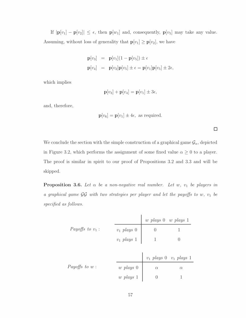
If |p[v1] − p[v2]| ≤ ǫ, then p[w1] and, consequently, p[v5] may take any value.
Assuming, without loss of generality that p[v1] ≥ p[v2], we have
p[v3] = p[v1](1 − p[v5]) ± ǫ
p[v4] = p[v2]p[v5] ± ǫ = p[v1]p[v5] ± 2ǫ,
which implies
p[v3] + p[v4] = p[v1] ± 3ǫ,
and, therefore,
p[v6] = p[v1] ± 4ǫ, as required.
We conclude the section with the simple construction of a graphical game Gα, depicted
in Figure 3.2, which performs the assignment of some fixed value α ≥ 0 to a player.
The proof is similar in spirit to our proof of Propositions 3.2 and 3.3 and will be
skipped.
Proposition 3.6. Let α be a non-negative real number. Let w, v1 be players in
a graphical game GG with two strategies per player and let the payoffs to w, v1 be
specified as follows.
Payoffs to v1 :
w plays 0 w plays 1
v1 plays 0 0 1
v1 plays 1 1 0
Payoffs to w :
v1 plays 0 v1 plays 1
w plays 0 α α
w plays 1 0 1
57
Then, for ǫ < 1, in every ǫ-Nash equilibrium of game GG, p[v1] = min(α, 1) ± ǫ. In
particular, in every Nash equilibrium of GG, p[v1] = min(α, 1).
Before concluding the section we give a useful definition.
Definition 3.7. Let v1, v2, . . . , vk, v be players of a graphical game Gf such that, in ev-
ery Nash equilibrium, it holds that p[v] = f(p[v1], . . . ,p[vk]), where f is some function
with k arguments and range [0, 1]. We say that the game Gf has error amplification
at most c if, in every ǫ-Nash equilibrium, it holds that p[v] = f(p[v1], . . . ,p[vk])± cǫ.
In particular, the games G=, G+, G−, G∗, Gα described above have error amplifications
at most 1, whereas the game Gmax has error amplification at most 4.
3.2 Reducing Graphical Games to Normal-Form
Games
We establish a mapping from graphical games to normal-form games as specified by
the following theorem.
Theorem 3.8. For every d > 1, a graphical game (directed or undirected) GG of
maximum degree d can be mapped in polynomial time to a (d2 + 1)-player normal-
form game G so that there is a polynomial-time computable surjective mapping g from
the Nash equilibria of the latter to the Nash equilibria of the former.
Proof.
Overview:
Figure 3.5 shows the construction of G = f(GG). We will explain the construction
in detail as well as show that it can be computed in polynomial time. We will also
establish that there is a surjective mapping from the Nash equilibria of G to the
Nash equilibria of GG. In the following discussion we will refer to the players of the
58
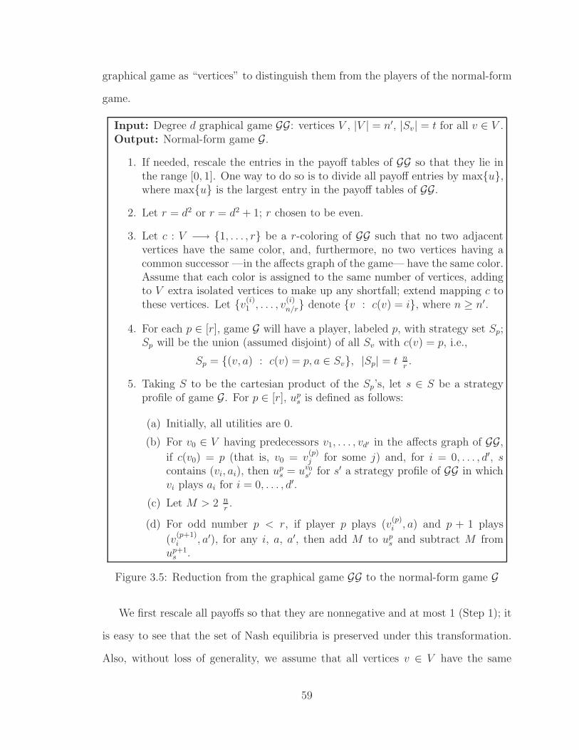
graphical game as “vertices” to distinguish them from the players of the normal-form
game.
Input: Degree d graphical game GG: vertices V , |V | = n′, |Sv| = t for all v ∈ V .Output: Normal-form game G.
1. If needed, rescale the entries in the payoff tables of GG so that they lie inthe range [0, 1]. One way to do so is to divide all payoff entries by maxu,where maxu is the largest entry in the payoff tables of GG.
2. Let r = d2 or r = d2 + 1; r chosen to be even.
3. Let c : V −→ 1, . . . , r be a r-coloring of GG such that no two adjacentvertices have the same color, and, furthermore, no two vertices having acommon successor —in the affects graph of the game— have the same color.Assume that each color is assigned to the same number of vertices, addingto V extra isolated vertices to make up any shortfall; extend mapping c tothese vertices. Let v(i)
1 , . . . , v(i)n/r denote v : c(v) = i, where n ≥ n′.
4. For each p ∈ [r], game G will have a player, labeled p, with strategy set Sp;Sp will be the union (assumed disjoint) of all Sv with c(v) = p, i.e.,
Sp = (v, a) : c(v) = p, a ∈ Sv, |Sp| = t nr.
5. Taking S to be the cartesian product of the Sp’s, let s ∈ S be a strategyprofile of game G. For p ∈ [r], up
s is defined as follows:
(a) Initially, all utilities are 0.
(b) For v0 ∈ V having predecessors v1, . . . , vd′ in the affects graph of GG,
if c(v0) = p (that is, v0 = v(p)j for some j) and, for i = 0, . . . , d′, s
contains (vi, ai), then ups = uv0
s′ for s′ a strategy profile of GG in whichvi plays ai for i = 0, . . . , d′.
(c) Let M > 2 nr.
(d) For odd number p < r, if player p plays (v(p)i , a) and p + 1 plays
(v(p+1)i , a′), for any i, a, a′, then add M to up
s and subtract M fromup+1
s .
Figure 3.5: Reduction from the graphical game GG to the normal-form game G
We first rescale all payoffs so that they are nonnegative and at most 1 (Step 1); it
is easy to see that the set of Nash equilibria is preserved under this transformation.
Also, without loss of generality, we assume that all vertices v ∈ V have the same
59
number of strategies, |Sv| = t. We color the vertices of G, where G = (V, E) is the
affects graph of GG, so that any two adjacent vertices have different colors, but also
any two vertices with a common successor have different colors (Step 3). Since this
type of coloring will be important for our discussion we will define it formally.
Definition 3.9. Let GG be a graphical game with affects graph G = (V, E). We
say that GG can be legally colored with k colors if there exists a mapping c : V →
1, 2, . . . , k such that, for all e = (v, u) ∈ E, c(v) 6= c(u) and, moreover, for all
e1 = (v, w), e2 = (u, w) ∈ E with v 6= u, c(v) 6= c(u). We call such coloring a legal
k-coloring of GG.
To get such coloring, it is sufficient to color the union of the underlying undirected
graph G′ with its square (with self-loops removed) so that no adjacent vertices have
the same color; this can be done with at most d2 colors —see, e.g., [CKK+00]— since
G′ has degree d by assumption; we are going to use r = d2 or r = d2 + 1 colors,
whichever is even, for reasons to become clear shortly. We assume for simplicity that
each color class has the same number of vertices, adding dummy vertices if needed
to satisfy this property. Henceforth, we assume that n is an integer multiple of r so
that every color class has nr
vertices.
We construct a normal-form game G with r ≤ d2 + 1 players. Each of them
corresponds to a color and has tnr
strategies, the t strategies of each of the nr
vertices
in its color class (Step 4). Since r is even, we can divide the r players into pairs and
make each pair play a generalized Matching Pennies game (see Definition 3.10 below)
at very high stakes, so as to ensure that all players will randomize uniformly over the
vertices assigned to them. 2 Within the set of strategies associated with each vertex,
the Matching Pennies game expresses no preference, and payoffs are augmented to
correspond to the payoffs that would arise in the original graphical game GG (see
2A similar trick is used in Theorem 7.3 of [SV06], a hardness result for a class of circuit games.
60
Step 5 for the exact specification of the payoffs).
Definition 3.10. The (2-player) game Generalized Matching Pennies is defined as
follows. Call the 2 players the pursuer and the evader, and let [n] denote their strate-
gies. If for any i ∈ [n] both players play i, then the pursuer receives a positive payoff
u > 0 and the evader receives a payoff of −u. Otherwise both players receive 0. It is
not hard to check that the game has a unique Nash equilibrium in which both players
use the uniform distribution.
Polynomial size of G = f(GG):
The input size is |GG| = Θ(n′ · td+1 · q), where n′ is the number of vertices in GG
and q the size of the values in the payoff matrices in the logarithmic cost model. The
normal-form game G has r ∈ d2, d2 + 1 players, each having tn/r strategies, where
n ≤ rn′ is the number of vertices in GG after the possible addition of dummy vertices
to make sure that all color classes have the same number of vertices. Hence, there are
r ·(tn/r
)r
≤(
(d2 + 1)(tn′)d2+1
)payoff entries in G. This is polynomial in |GG| so
long as d is constant. Moreover, each payoff entry will be of polynomial size since M
is of polynomial size and each payoff entry of the game G is the sum of 0 or M and
a payoff entry of GG.
Construction of the mapping g:
Given a Nash equilibrium NG = xp(v,a)p,v,a of G = f(GG), we claim that we can
recover a Nash equilibrium xvav,a of GG, NGG = g(NG), as follows:
xva := x
c(v)(v,a)
/∑
j∈Sv
xc(v)(v,j), ∀a ∈ Sv, v ∈ V. (3.1)
Clearly g is computable in polynomial time.
Proof that g maps Nash equilibria of G to Nash equilibria of GG:
Call GG′ the graphical game resulting from GG by rescaling the utilities so that
61
they lie in the range [0, 1]. It is easy to see that any Nash equilibrium of game GG
is, also, a Nash equilibrium of game GG′ and vice versa. Therefore, it is enough
to establish that the mapping g maps every Nash equilibrium of game G to a Nash
equilibrium of game GG′.
For v ∈ V , c(v) = p, let “p plays v” denote the event that p plays (v, a) for some
a ∈ Sv. We show that in a Nash equilibrium NG of game G, for every player p and
every v ∈ V with c(v) = p, Pr[p plays v] ∈ [λ − 1M
, λ + 1M
], where λ =(
nr
)−1. Note
that the “fair share” for v is λ.
Lemma 3.11. For all v ∈ V , in a Nash equilibrium of G, Pr[c(v) plays v] ∈ [λ −1M
, λ + 1M
].
Proof. Suppose, for a contradiction, that in a Nash equilibrium of G, Pr[p plays v
(p)i
]<
λ− 1M
for some i, p. Then there exists some j such that Pr[p plays v
(p)j
]> λ + 1
Mλ.
If p is odd (a pursuer) then p+1 (the evader) will have utility of at least −λM+1 for
playing any strategy(v
(p+1)i , a
), a ∈ S
v(p+1)i
, whereas utility of at most −λM−λ+1 for
playing any strategy (v(p+1)j , a), a ∈ S
v(p+1)j
. Since −λM +1 > −λM−λ+1, in a Nash
equilibrium, Pr[p + 1 plays v
(p+1)j
]= 0. Therefore, there exists some k such that
Pr[p + 1 plays v
(p+1)k
]> λ. Now the payoff of p for playing any strategy
(v
(p)j , a
),
a ∈ Sv(p)j
, is at most 1, whereas the payoff for playing any strategy(v
(p)k , a
), a ∈ S
v(p)k
is at least λM . Thus, in a Nash equilibrium, player p should not include any strategy(v
(p)j , a
), a ∈ S
v(p)j
, in her support; hence Pr[p plays v
(p)j
]= 0, a contradiction.
If p is even, then p−1 will have utility of at most (λ− 1M
)M+1 for playing any strat-
egy(v
(p−1)i , a
), a ∈ S
v(p−1)i
, whereas utility of at least (λ+ 1M
λ)M for playing any strat-
egy (v(p−1)j , a), a ∈ S
v(p−1)j
. Hence, in a Nash equilibrium Pr[p − 1 plays v
(p−1)i
]= 0,
which implies that there exists some k such that Pr[p − 1 plays v
(p−1)k
]> λ. But,
p will then have utility of at least 0 for playing any strategy(v
(p)i , a
), a ∈ S
v(p)i
,
whereas utility of at most −λM + 1 for playing any strategy (v(p)k , a), a ∈ S
v(p)k
. Since
62
0 > −λM + 1, in a Nash equilibrium, Pr[p plays v
(p)k
]= 0. Therefore, there exists
some k′ such that Pr[p plays v
(p)k′
]> λ. Now the payoff of p − 1 for playing any
strategy(v
(p−1)k , a
), a ∈ S
v(p−1)k
, is at most 1, whereas the payoff for playing any
strategy(v
(p−1)k′ , a
), a ∈ S
v(p−1)
k′is at least λM . Thus, in a Nash equilibrium, player
p − 1 should not include any strategy(v
(p−1)k , a
), a ∈ S
v(p−1)k
, in her support; hence
Pr[p − 1 plays v
(p−1)k
]= 0, a contradiction.
From the above discussion, it follows that every vertex is chosen with probability
at least λ− 1M
by the player that represents its color class. A similar argument shows
that no vertex is chosen with probability greater than λ + 1M
. Indeed, suppose, for
a contradiction, that in a Nash equilibrium of G, Pr[p plays v
(p)j
]> λ + 1
Mfor some
j, p; then there exists some i such that Pr[p plays v
(p)i
]< λ − 1
Mλ; now, distinguish
two cases depending on whether p is even or odd and proceed in the same fashion as
in the argument used above to show that no vertex is chosen with probability smaller
than λ − 1/M .
To see that xvav,a, defined by (3.1), corresponds to a Nash equilibrium of GG′
note that, for any player p and vertex v ∈ V such that c(v) = p, the division of
Pr[p plays v] into Pr[p plays (v, a)], for various values of a ∈ Sv, is driven entirely
by the same payoffs as in GG′; moreover, note that there is some positive probability
p(v) ≥ (λ − 1M
)d > 0 that the predecessors of v are chosen by the other players of
G and the additional expected payoff to p resulting from choosing (v, a), for some
a ∈ Sv, is p(v) times the expected payoff of v in GG′ if v chooses action a and all
other vertices play as specified by (3.1). More formally, suppose that p = c(v) for
some vertex v of the graphical game GG′ and, without loss of generality, assume that
p is odd (pursuer) and that v is the vertex v(p)i in the notation of Figure 3.5. Then, in
a Nash equilibrium of the game G, we have, by the definition of a Nash equilibrium,
63
that for all strategies a, a′ ∈ Sv of vertex v:
E [payoff to p for playing (v, a)] > E [payoff to p for playing (v, a′)] ⇒ xp(v,a′) = 0.
(3.2)
But
E [payoff to p for playing (v, a)] =
M · Pr[p + 1 plays v
(p+1)i
]+
∑
s∈SN (v)\v
uvas
∏
u∈N (v)\vx
c(u)(u,su)
and, similarly, for a′. Therefore, (3.2) implies
∑
s∈SN (v)\v
uvas
∏
u∈N (v)\vx
c(u)(u,su) >
∑
s∈SN (v)\v
uva′s
∏
u∈N (v)\vx
c(u)(u,su) ⇒ xp
(v,a′) = 0.
Dividing by∏
u∈N (v)\v∑
j∈Sux
c(u)(u,j) =
∏u∈N (v)\v Pr [c(u) plays u] = p(v) and in-
voking (3.1) gives
∑
s∈SN (v)\v
uvas
∏
u∈N (v)\vxu
su>
∑
s∈SN (v)\v
uva′s
∏
u∈N (v)\vxu
su⇒ xv
a′ = 0,
where we used that p(v) ≥ (λ − 1M
)d > 0, which follows by Lemma 3.11.
Mapping g is surjective on the Nash equilibria of GG′ and, therefore, GG:
We will show that, for every Nash equilibrium NGG′ = xvav,a of GG′, there exists
a Nash equilibrium NG = xp(v,a)p,v,a of G such that (3.1) holds. The existence can
be easily established via the existence of a Nash equilibrium in a game G′ defined as
follows. Suppose that, in NGG′, every vertex v ∈ V receives an expected payoff of
uv from every strategy in the support of xvaa. Define the following game G′ whose
structure results from G by merging the strategies (v, a)a of player p = c(v) into
64
one strategy spv, for every v such that c(v) = p. So the strategy set of player p in G′
will be spv | c(v) = p also denoted as s(p)
1 , . . . , s(p)n/r for ease of notation. Define
now the payoffs to the players as follows. Initialize the payoff matrices with all entries
equal to 0. For every strategy profile s,
• for v0 ∈ V having predecessors v1, . . . , vd′ in the affects graph of GG′, if, for
i = 0, . . . , d′, s contains sc(vi)vi , then add uv0 to u
c(v0)s .
• for odd number p < r if player p plays strategy s(p)i and player p+1 plays strategy
s(p+1)i then add M to up
s and subtract M from up+1s (Generalized Matching
Pennies).
Note the similarity between the definitions of the payoff matrices of G and G′. From
Nash’s theorem, game G′ has a Nash equilibrium ypspvp,v and it is not hard to verify
that xp(v,a)p,v,a is a Nash equilibrium of game G, where xp
(v,a) := ypspv· xv
a, for all p,
v ∈ V such that c(v) = p, and a ∈ Sv.
3.3 Reducing Normal-Form Games to Graphical
Games
We establish the following mapping from normal-form games to graphical games.
Theorem 3.12. For every r > 1, a normal-form game with r players can be mapped
in polynomial time to an undirected graphical game of maximum degree 3 and two
strategies per player so that there is a polynomial-time computable surjective mapping
g from the Nash equilibria of the latter to the Nash equilibria of the former.
65
Given a normal-form game G having r players, 1, . . . , r, and n strategies per player,
say Sp = [n] for all p ∈ [r], we will construct a graphical game GG, with a bipartite
graph of maximum degree 3, and 2 strategies per player, say 0, 1, with description
length polynomial in the description length of G, so that from every Nash equilibrium
of GG we can recover a Nash equilibrium of G. In the following discussion we will
refer to the players of the graphical game as “vertices” to distinguish them from the
players of the normal-form game. It will be easy to check that the graph of GG is
bipartite and has degree 3; this graph will be denoted G = (V ∪W, E), where W and
V are disjoint, and each edge in E goes between V and W . For every vertex v of the
graphical game, we will denote by p[v] the probability that v plays pure strategy 1.
Recall that G is specified by the quantities ups : p ∈ [r], s ∈ S. A mixed strategy
profile of G is given by probabilities xpj : p ∈ [r], j ∈ Sp. GG will contain a vertex
v(xpj ) ∈ V for each player p and strategy j ∈ Sp, and the construction of GG will
ensure that in any Nash equilibrium of GG, the quantities p[v(xpj )] : p ∈ [r], j ∈ Sp,
if interpreted as values xpjp,j, will constitute a Nash equilibrium of G. Extending
this notation, for various arithmetic expressions A involving any xpj and up
s, vertex
v(A) ∈ V will be used, and be constructed such that in any Nash equilibrium of GG,
p[v(A)] is equal to A evaluated at the given values of ups and with xp
j equal to p[v(xpj )].
Elements of W are used to mediate between elements of V , so that the latter ones
obey the intended arithmetic relationships.
We use Propositions 3.2-3.6 as building blocks of GG, starting with r subgraphs
that represent mixed strategies for the players of G. In the following, we construct
a graphical game containing vertices v(xpj)j∈[n], whose probabilities sum to 1, and
internal vertices vpj , which control the distribution of the one unit of probability mass
among the vertices v(xpj ). See Figure 3.6 for an illustration.
Proposition 3.13. Consider a graphical game that contains
66
• for j ∈ [n] a vertex v(xpj )
• for j ∈ [n − 1] a vertex vpj
• for j ∈ [n] a vertex v(∑j
i=1 xpi )
• for j ∈ [n−1] a vertex wj(p) used to ensure p[v(∑j
i=1 xpi )] = p[v(
∑j+1i=1 xp
i )](1−
p[vpj ])
• for j ∈ [n − 1] a vertex w′j(p) used to ensure p[v(xp
j+1)] = p[v(∑j+1
i=1 xpi )]p[vp
j ]
• a vertex w′0(p) used to ensure p[v(xp
1)] = p[v(∑1
i=1 xpi )]
Also, let v(∑n
i=1 xpi ) have payoff of 1 when it plays 1 and 0 otherwise. Then, in any
Nash equilibrium of the graphical game,∑n
i=1 p[v(xpi )] = 1 and moreover p[v(
∑ji=1 xp
i )] =∑j
i=1 p[v(xpi )], and the graph is bipartite and of degree 3.
Proof. It is not hard to verify that the graph has degree 3. Most of the degree
3 vertices are the w vertices used in Propositions 3.2 and 3.3 to connect the pairs
or triples of graph players whose probabilities are supposed to obey an arithmetic
relationship. In a Nash equilibrium, v(∑n
i=1 xpi ) plays 1. The vertices vp
j split the
probability p[v(∑j+1
i=1 xpi )] between p[v(
∑ji=1 xp
i )] and p[v(xpj+1)].
Comment. The values p[vpj ] control the distribution of probability (summing to 1)
amongst the n vertices v(xpj). These vertices can set to zero any proper subset of the
probabilities p[v(xpj )].
Notation. For s ∈ S−p let xs = x1s1
· x2s2· · ·xp−1
sp−1· xp+1
sp+1· · ·xr
sr. Also, let Up
j =∑
s∈S−pup
jsxs be the utility to p for playing j in the context of a given mixed profile
xss∈S−p.
Lemma 3.14. Suppose all utilities ups (of G) lie in the range [0, 1] for some p ∈ [r].
We can construct a degree 3 bipartite graph having a total of O(rnr) vertices, including
67
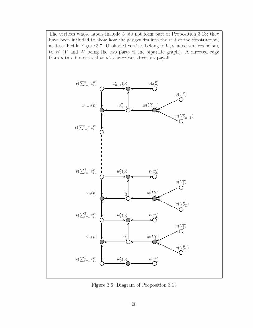
The vertices whose labels include U do not form part of Proposition 3.13; theyhave been included to show how the gadget fits into the rest of the construction,as described in Figure 3.7. Unshaded vertices belong to V , shaded vertices belongto W (V and W being the two parts of the bipartite graph). A directed edgefrom u to v indicates that u’s choice can affect v’s payoff.
v(∑n
i=1 xpi ) w′
n−1(p) v(xpn)
v(Upn)
wn−1(p) vpn−1 w(Up
n−1)
v(Up≤n−1)
v(∑n−1
i=1 xpi )
v(∑3
i=1 xpi ) w′
2(p) v(xp3)
v(Up3 )
w2(p) vp2 w(Up
2 )
v(Up≤2)
v(∑2
i=1 xpi ) w′
1(p) v(xp2)
v(Up2 )
w1(p) vp1 w(Up
1 )
v(Up≤1)
v(∑1
i=1 xpi ) w′
0(p) v(xp1)
Figure 3.6: Diagram of Proposition 3.13
68
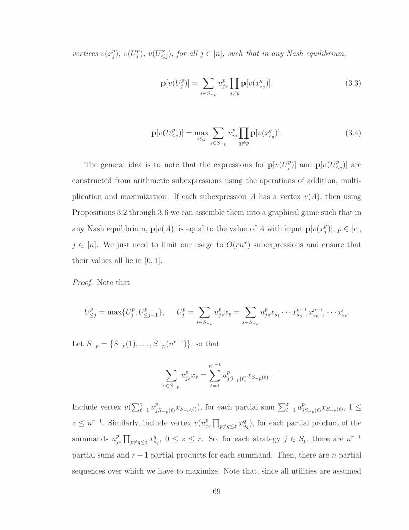
vertices v(xpj ), v(Up
j ), v(Up≤j), for all j ∈ [n], such that in any Nash equilibrium,
p[v(Upj )] =
∑
s∈S−p
upjs
∏
q 6=p
p[v(xqsq
)], (3.3)
p[v(Up≤j)] = max
i≤j
∑
s∈S−p
upis
∏
q 6=p
p[v(xqsq
)]. (3.4)
The general idea is to note that the expressions for p[v(Upj )] and p[v(Up
≤j)] are
constructed from arithmetic subexpressions using the operations of addition, multi-
plication and maximization. If each subexpression A has a vertex v(A), then using
Propositions 3.2 through 3.6 we can assemble them into a graphical game such that in
any Nash equilibrium, p[v(A)] is equal to the value of A with input p[v(xpj )], p ∈ [r],
j ∈ [n]. We just need to limit our usage to O(rnr) subexpressions and ensure that
their values all lie in [0, 1].
Proof. Note that
Up≤j = maxUp
j , Up≤j−1, Up
j =∑
s∈S−p
upjsxs =
∑
s∈S−p
upjsx
1s1· · ·xp−1
sp−1xp+1
sp+1· · ·xr
sr.
Let S−p = S−p(1), . . . , S−p(nr−1), so that
∑
s∈S−p
upjsxs =
nr−1∑
ℓ=1
upjS−p(ℓ)xS−p(ℓ).
Include vertex v(∑z
ℓ=1 upjS−p(ℓ)xS−p(ℓ)), for each partial sum
∑zℓ=1 up
jS−p(ℓ)xS−p(ℓ), 1 ≤
z ≤ nr−1. Similarly, include vertex v(upjs
∏p 6=q≤z xq
sq), for each partial product of the
summands upjs
∏p 6=q≤z xq
sq, 0 ≤ z ≤ r. So, for each strategy j ∈ Sp, there are nr−1
partial sums and r + 1 partial products for each summand. Then, there are n partial
sequences over which we have to maximize. Note that, since all utilities are assumed
69
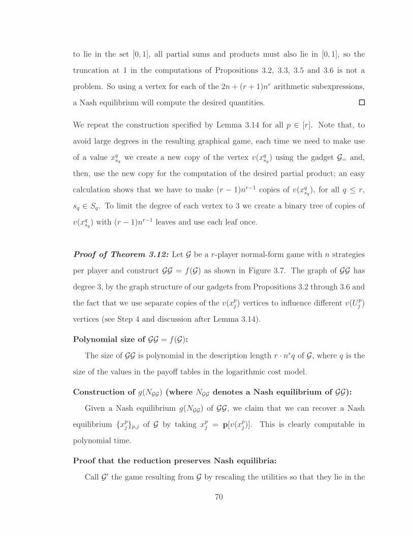
to lie in the set [0, 1], all partial sums and products must also lie in [0, 1], so the
truncation at 1 in the computations of Propositions 3.2, 3.3, 3.5 and 3.6 is not a
problem. So using a vertex for each of the 2n + (r + 1)nr arithmetic subexpressions,
a Nash equilibrium will compute the desired quantities.
We repeat the construction specified by Lemma 3.14 for all p ∈ [r]. Note that, to
avoid large degrees in the resulting graphical game, each time we need to make use
of a value xqsq
we create a new copy of the vertex v(xqsq
) using the gadget G= and,
then, use the new copy for the computation of the desired partial product; an easy
calculation shows that we have to make (r − 1)nr−1 copies of v(xqsq
), for all q ≤ r,
sq ∈ Sq. To limit the degree of each vertex to 3 we create a binary tree of copies of
v(xqsq
) with (r − 1)nr−1 leaves and use each leaf once.
Proof of Theorem 3.12: Let G be a r-player normal-form game with n strategies
per player and construct GG = f(G) as shown in Figure 3.7. The graph of GG has
degree 3, by the graph structure of our gadgets from Propositions 3.2 through 3.6 and
the fact that we use separate copies of the v(xpj ) vertices to influence different v(Up
j )
vertices (see Step 4 and discussion after Lemma 3.14).
Polynomial size of GG = f(G):
The size of GG is polynomial in the description length r · nrq of G, where q is the
size of the values in the payoff tables in the logarithmic cost model.
Construction of g(NGG) (where NGG denotes a Nash equilibrium of GG):
Given a Nash equilibrium g(NGG) of GG, we claim that we can recover a Nash
equilibrium xpjp,j of G by taking xp
j = p[v(xpj )]. This is clearly computable in
polynomial time.
Proof that the reduction preserves Nash equilibria:
Call G′ the game resulting from G by rescaling the utilities so that they lie in the
70
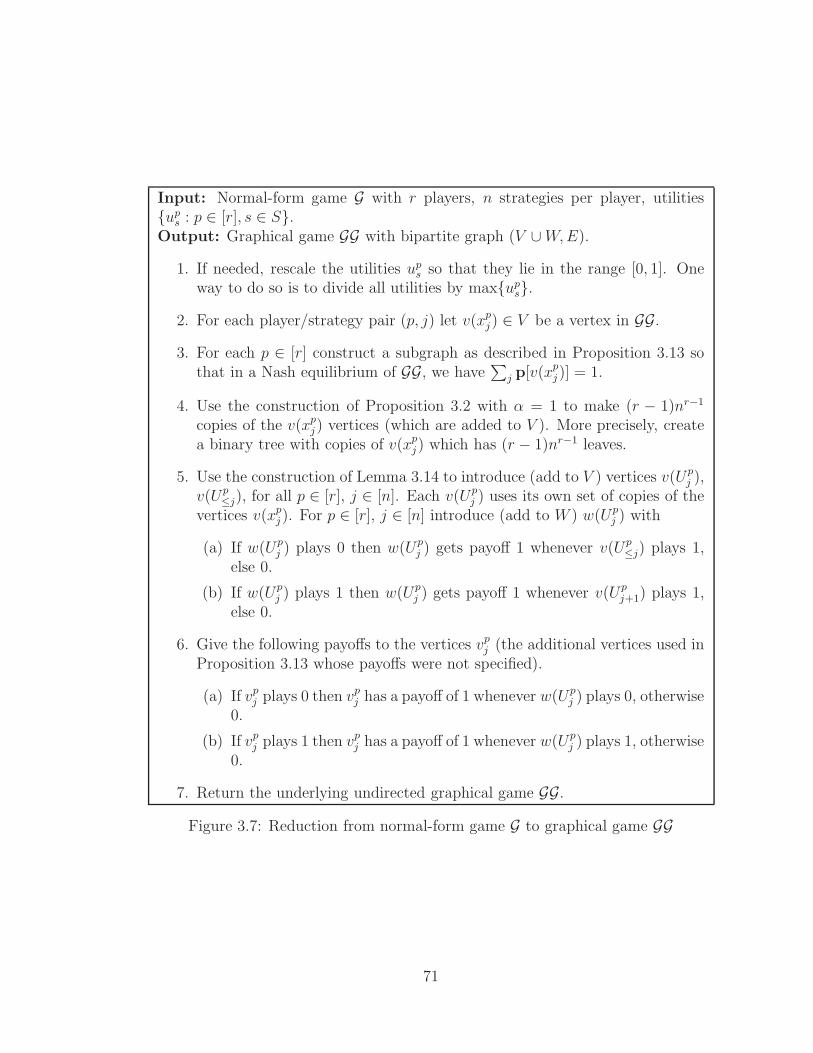
Input: Normal-form game G with r players, n strategies per player, utilitiesup
s : p ∈ [r], s ∈ S.Output: Graphical game GG with bipartite graph (V ∪ W, E).
1. If needed, rescale the utilities ups so that they lie in the range [0, 1]. One
way to do so is to divide all utilities by maxups.
2. For each player/strategy pair (p, j) let v(xpj ) ∈ V be a vertex in GG.
3. For each p ∈ [r] construct a subgraph as described in Proposition 3.13 sothat in a Nash equilibrium of GG, we have
∑j p[v(xp
j )] = 1.
4. Use the construction of Proposition 3.2 with α = 1 to make (r − 1)nr−1
copies of the v(xpj ) vertices (which are added to V ). More precisely, create
a binary tree with copies of v(xpj ) which has (r − 1)nr−1 leaves.
5. Use the construction of Lemma 3.14 to introduce (add to V ) vertices v(Upj ),
v(Up≤j), for all p ∈ [r], j ∈ [n]. Each v(Up
j ) uses its own set of copies of thevertices v(xp
j ). For p ∈ [r], j ∈ [n] introduce (add to W ) w(Upj ) with
(a) If w(Upj ) plays 0 then w(Up
j ) gets payoff 1 whenever v(Up≤j) plays 1,
else 0.
(b) If w(Upj ) plays 1 then w(Up
j ) gets payoff 1 whenever v(Upj+1) plays 1,
else 0.
6. Give the following payoffs to the vertices vpj (the additional vertices used in
Proposition 3.13 whose payoffs were not specified).
(a) If vpj plays 0 then vp
j has a payoff of 1 whenever w(Upj ) plays 0, otherwise
0.
(b) If vpj plays 1 then vp
j has a payoff of 1 whenever w(Upj ) plays 1, otherwise
0.
7. Return the underlying undirected graphical game GG.
Figure 3.7: Reduction from normal-form game G to graphical game GG
71
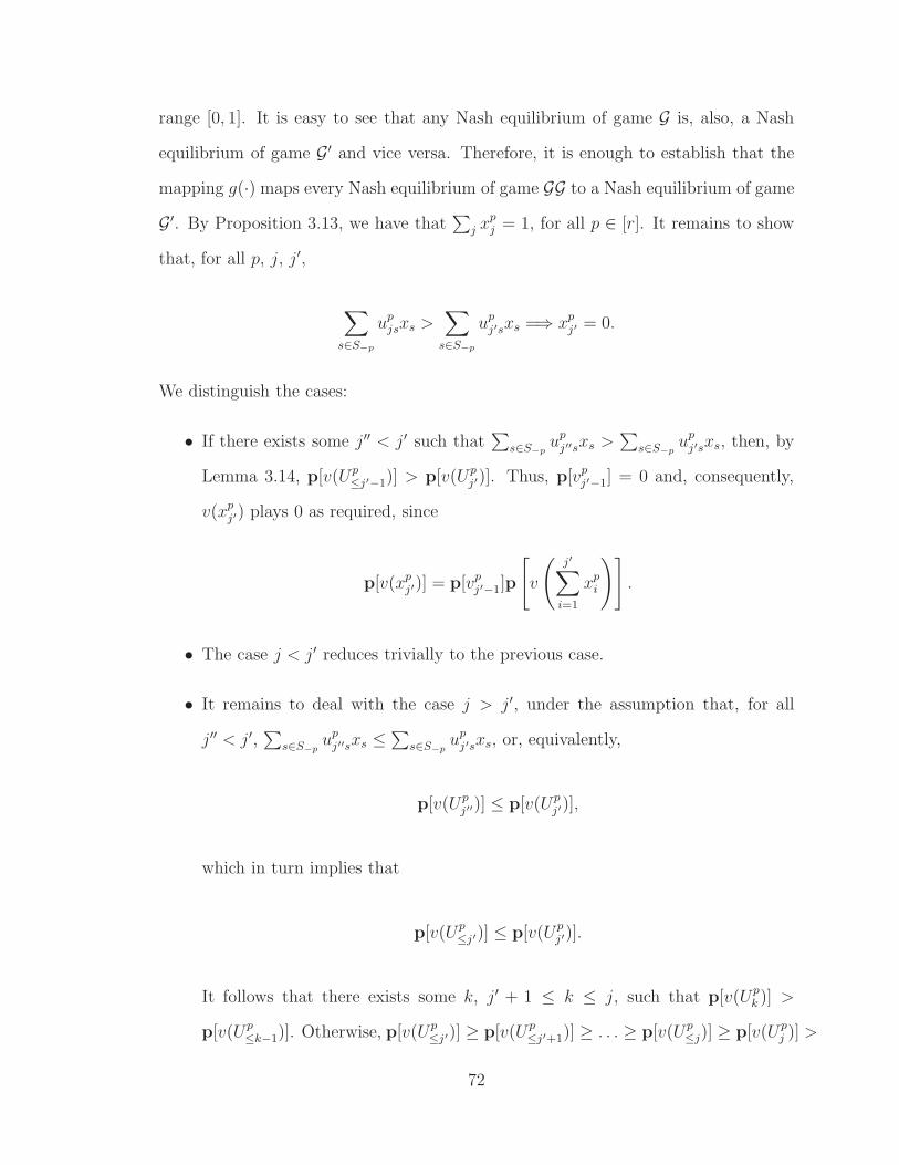
range [0, 1]. It is easy to see that any Nash equilibrium of game G is, also, a Nash
equilibrium of game G′ and vice versa. Therefore, it is enough to establish that the
mapping g(·) maps every Nash equilibrium of game GG to a Nash equilibrium of game
G′. By Proposition 3.13, we have that∑
j xpj = 1, for all p ∈ [r]. It remains to show
that, for all p, j, j′,
∑
s∈S−p
upjsxs >
∑
s∈S−p
upj′sxs =⇒ xp
j′ = 0.
We distinguish the cases:
• If there exists some j′′ < j′ such that∑
s∈S−pup
j′′sxs >∑
s∈S−pup
j′sxs, then, by
Lemma 3.14, p[v(Up≤j′−1)] > p[v(Up
j′)]. Thus, p[vpj′−1] = 0 and, consequently,
v(xpj′) plays 0 as required, since
p[v(xpj′)] = p[vp
j′−1]p
[v
(j′∑
i=1
xpi
)].
• The case j < j′ reduces trivially to the previous case.
• It remains to deal with the case j > j′, under the assumption that, for all
j′′ < j′,∑
s∈S−pup
j′′sxs ≤∑
s∈S−pup
j′sxs, or, equivalently,
p[v(Upj′′)] ≤ p[v(Up
j′)],
which in turn implies that
p[v(Up≤j′)] ≤ p[v(Up
j′)].
It follows that there exists some k, j′ + 1 ≤ k ≤ j, such that p[v(Upk )] >
p[v(Up≤k−1)]. Otherwise, p[v(Up
≤j′)] ≥ p[v(Up≤j′+1)] ≥ . . . ≥ p[v(Up
≤j)] ≥ p[v(Upj )] >
72

p[v(Upj′)], which is a contradiction to p[v(Up
≤j′)] ≤ p[v(Upj′)]. Since p[v(Up
k )] >
p[v(Up≤k−1)], it follows that p[w(Up
k−1)] = 1 ⇒ p[vpk−1] = 1 and, therefore,
p
[v
(k−1∑
i=1
xpi
)]= p
[v
(k∑
i=1
xpi
)](1 − p[vp
k−1]) = 0
⇒ p
[v
(j′∑
i=1
xpi
)]= 0 ⇒ p
[v(xp
j′)]
= 0.
Mapping g is surjective on the Nash equilibria of G′ and, therefore, G:
We will show that given a Nash equilibrium NG′ of G′ there is a Nash equilibrium
NGG of GG such that g(NGG) = NG′. Let NG′ = xpj : p ≤ r, j ∈ Sp. In NGG, let
p[v(xpj )] = xp
j . Lemma 3.14 shows that the values p[v(Upj )] are the expected utilities
to player p for playing strategy j, given that all other players use the mixed strategy
xpj : p ≤ r, j ∈ Sp. We identify values for p[vp
j ] that complete a Nash equilibrium
for GG.
Based on the payoffs to vpj described in Figure 3.7 we have
• If p[v(Up≤j)] > p[v(Up
j+1)] then p[w(Upj )] = 0; p[vp
j ] = 0;
• If p[v(Up≤j)] < p[v(Up
j+1)] then p[w(Upj )] = 1; p[vp
j ] = 1;
• If p[v(Up≤j)] = p[v(Up
j+1)] then choose p[w(Upj )] = 1
2; p[vp
j ] is arbitrary (we may
assign it any value)
Given the above constraints on the values p[vpj ] we must check that we can choose
them (and there is a unique choice) so as to make them consistent with the prob-
abilities p[v(xpj )]. We use the fact the values xp
j form a Nash equilibrium of G. In
particular, we know that p[v(xpj )] = 0 if there exists j′ with Up
j′ > Upj . We claim that
73
for j satisfying p[v(Up≤j)] = p[v(Up
j+1)], if we choose
p[vpj ] = p[v(xp
j+1)]/
j+1∑
i=1
p[v(xpi )],
then the values p[v(xpj )] are consistent. 2
3.4 Combining the Reductions
Suppose that we take either a graphical or a normal-form game, and apply to it both
of the reductions described in the previous sections. Then we obtain a game of the
same type and a surjective mapping from the Nash equilibria of the latter to the Nash
equilibria of the former.
Corollary 3.15. For any fixed d, a (directed or undirected) graphical game of maxi-
mum degree d can be mapped in polynomial time to an undirected graphical game of
maximum degree 3 so that there is a polynomial-time computable surjective mapping
g from the Nash equilibria of the latter to the Nash equilibria of the former.
The following also follows directly from Theorems 3.12 and 3.8, but is not as
strong as Theorem 3.17 below.
Corollary 3.16. For any fixed r > 1, a r-player normal-form game can be mapped in
polynomial time to a 10-player normal-form game so that there is a polynomial-time
computable surjective mapping g from the Nash equilibria of the latter to the Nash
equilibria of the former.
Proof. Theorem 3.12 converts a r-player game G into a graphical game GG based on
a graph of degree 3. Theorem 3.8 converts GG to a 10-player game G′, whose Nash
equilibria encode the Nash equilibria of GG and hence of G. (Note that for d an odd
74

number, the proof of Theorem 3.8 implies a reduction to a (d2+1)-player normal-form
game.)
We next prove a stronger result, by exploiting in more detail the structure of the
graphical games GG constructed in the proof of Theorem 3.12. The technique used
here will be used in Section 3.5 to strengthen the result even further.
Theorem 3.17. For any fixed r > 1, a r-player normal-form game can be mapped in
polynomial time to a 4-player normal-form game so that there is a polynomial-time
computable surjective mapping g from the Nash equilibria of the latter to the Nash
equilibria of the former.
Proof. Construct G′ from G as shown in Figure 3.8.
Polynomial size of G′ = f(G).
By Theorem 3.12, GG (as constructed in Figure 3.8) is of polynomial size. The size
of GG′ is at most 3 times the size of GG since we do not need to apply Step 3 to any
edges that are themselves constructed by an earlier iteration of Step 3. Finally, the
size of G′ is polynomial in the size of GG′ from Theorem 3.8.
Construction of g(NG′) (for NG′ a Nash equilibrium of G′).
Let g1 be a surjective mapping from the Nash equilibria of GG to the Nash equilibria
of G, which is guaranteed to exist by Theorem 3.12. It is trivial to construct a
surjective mapping g2 from the Nash equilibria of GG′ to the Nash equilibria of GG.
By Theorem 3.8, there exists a surjective mapping g3 from the Nash equilibria of G′
to the Nash equilibria of GG′. Therefore, g3 g2 g1 is a surjective mapping from the
Nash equilibria of G′ to the Nash equilibria of G.
75
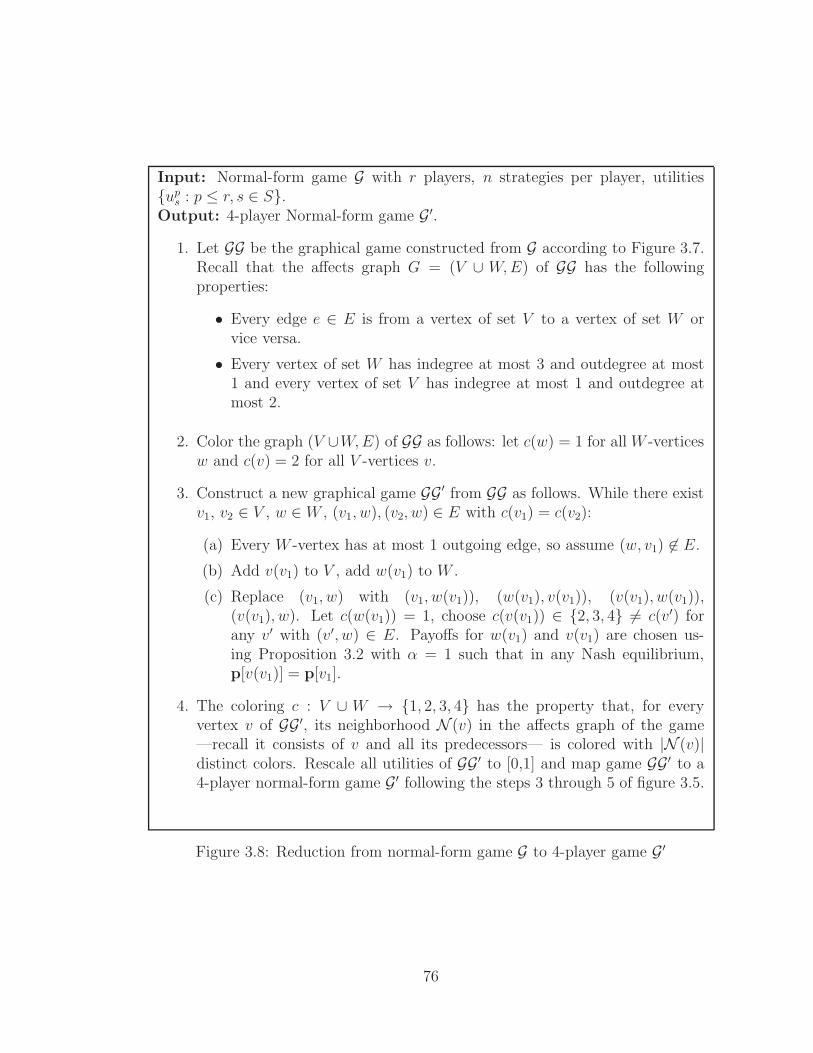
Input: Normal-form game G with r players, n strategies per player, utilitiesup
s : p ≤ r, s ∈ S.Output: 4-player Normal-form game G′.
1. Let GG be the graphical game constructed from G according to Figure 3.7.Recall that the affects graph G = (V ∪ W, E) of GG has the followingproperties:
• Every edge e ∈ E is from a vertex of set V to a vertex of set W orvice versa.
• Every vertex of set W has indegree at most 3 and outdegree at most1 and every vertex of set V has indegree at most 1 and outdegree atmost 2.
2. Color the graph (V ∪W, E) of GG as follows: let c(w) = 1 for all W -verticesw and c(v) = 2 for all V -vertices v.
3. Construct a new graphical game GG′ from GG as follows. While there existv1, v2 ∈ V , w ∈ W , (v1, w), (v2, w) ∈ E with c(v1) = c(v2):
(a) Every W -vertex has at most 1 outgoing edge, so assume (w, v1) 6∈ E.
(b) Add v(v1) to V , add w(v1) to W .
(c) Replace (v1, w) with (v1, w(v1)), (w(v1), v(v1)), (v(v1), w(v1)),(v(v1), w). Let c(w(v1)) = 1, choose c(v(v1)) ∈ 2, 3, 4 6= c(v′) forany v′ with (v′, w) ∈ E. Payoffs for w(v1) and v(v1) are chosen us-ing Proposition 3.2 with α = 1 such that in any Nash equilibrium,p[v(v1)] = p[v1].
4. The coloring c : V ∪ W → 1, 2, 3, 4 has the property that, for everyvertex v of GG′, its neighborhood N (v) in the affects graph of the game—recall it consists of v and all its predecessors— is colored with |N (v)|distinct colors. Rescale all utilities of GG′ to [0,1] and map game GG′ to a4-player normal-form game G′ following the steps 3 through 5 of figure 3.5.
Figure 3.8: Reduction from normal-form game G to 4-player game G′
76
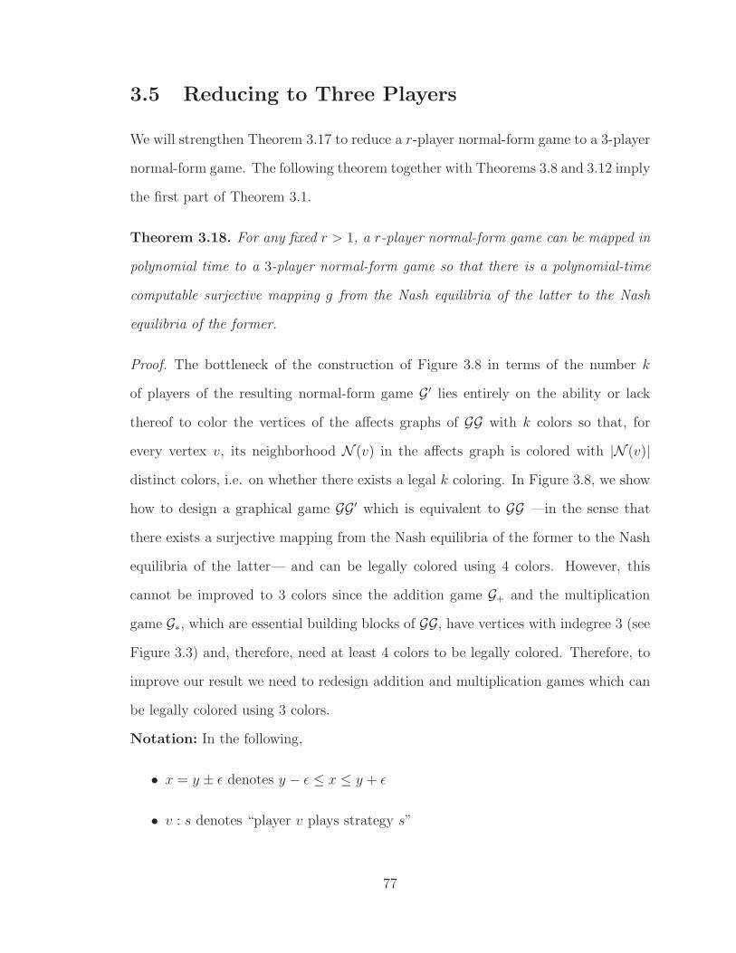
3.5 Reducing to Three Players
We will strengthen Theorem 3.17 to reduce a r-player normal-form game to a 3-player
normal-form game. The following theorem together with Theorems 3.8 and 3.12 imply
the first part of Theorem 3.1.
Theorem 3.18. For any fixed r > 1, a r-player normal-form game can be mapped in
polynomial time to a 3-player normal-form game so that there is a polynomial-time
computable surjective mapping g from the Nash equilibria of the latter to the Nash
equilibria of the former.
Proof. The bottleneck of the construction of Figure 3.8 in terms of the number k
of players of the resulting normal-form game G′ lies entirely on the ability or lack
thereof to color the vertices of the affects graphs of GG with k colors so that, for
every vertex v, its neighborhood N (v) in the affects graph is colored with |N (v)|
distinct colors, i.e. on whether there exists a legal k coloring. In Figure 3.8, we show
how to design a graphical game GG′ which is equivalent to GG —in the sense that
there exists a surjective mapping from the Nash equilibria of the former to the Nash
equilibria of the latter— and can be legally colored using 4 colors. However, this
cannot be improved to 3 colors since the addition game G+ and the multiplication
game G∗, which are essential building blocks of GG, have vertices with indegree 3 (see
Figure 3.3) and, therefore, need at least 4 colors to be legally colored. Therefore, to
improve our result we need to redesign addition and multiplication games which can
be legally colored using 3 colors.
Notation: In the following,
• x = y ± ǫ denotes y − ǫ ≤ x ≤ y + ǫ
• v : s denotes “player v plays strategy s”
77
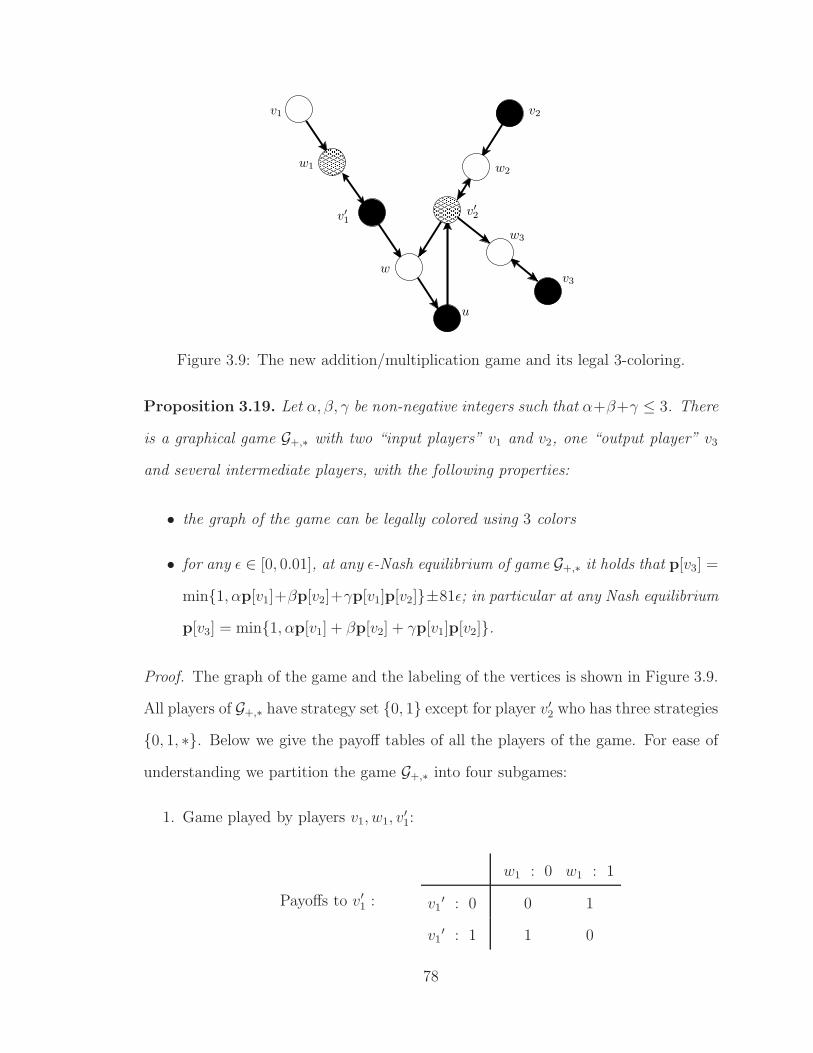
v′1
w2
v2
v′2
w3
v3
w
u
v1
w1
Figure 3.9: The new addition/multiplication game and its legal 3-coloring.
Proposition 3.19. Let α, β, γ be non-negative integers such that α+β+γ ≤ 3. There
is a graphical game G+,∗ with two “input players” v1 and v2, one “output player” v3
and several intermediate players, with the following properties:
• the graph of the game can be legally colored using 3 colors
• for any ǫ ∈ [0, 0.01], at any ǫ-Nash equilibrium of game G+,∗ it holds that p[v3] =
min1, αp[v1]+βp[v2]+γp[v1]p[v2]±81ǫ; in particular at any Nash equilibrium
p[v3] = min1, αp[v1] + βp[v2] + γp[v1]p[v2].
Proof. The graph of the game and the labeling of the vertices is shown in Figure 3.9.
All players of G+,∗ have strategy set 0, 1 except for player v′2 who has three strategies
0, 1, ∗. Below we give the payoff tables of all the players of the game. For ease of
understanding we partition the game G+,∗ into four subgames:
1. Game played by players v1, w1, v′1:
Payoffs to v′1 :
w1 : 0 w1 : 1
v1′ : 0 0 1
v1′ : 1 1 0
78
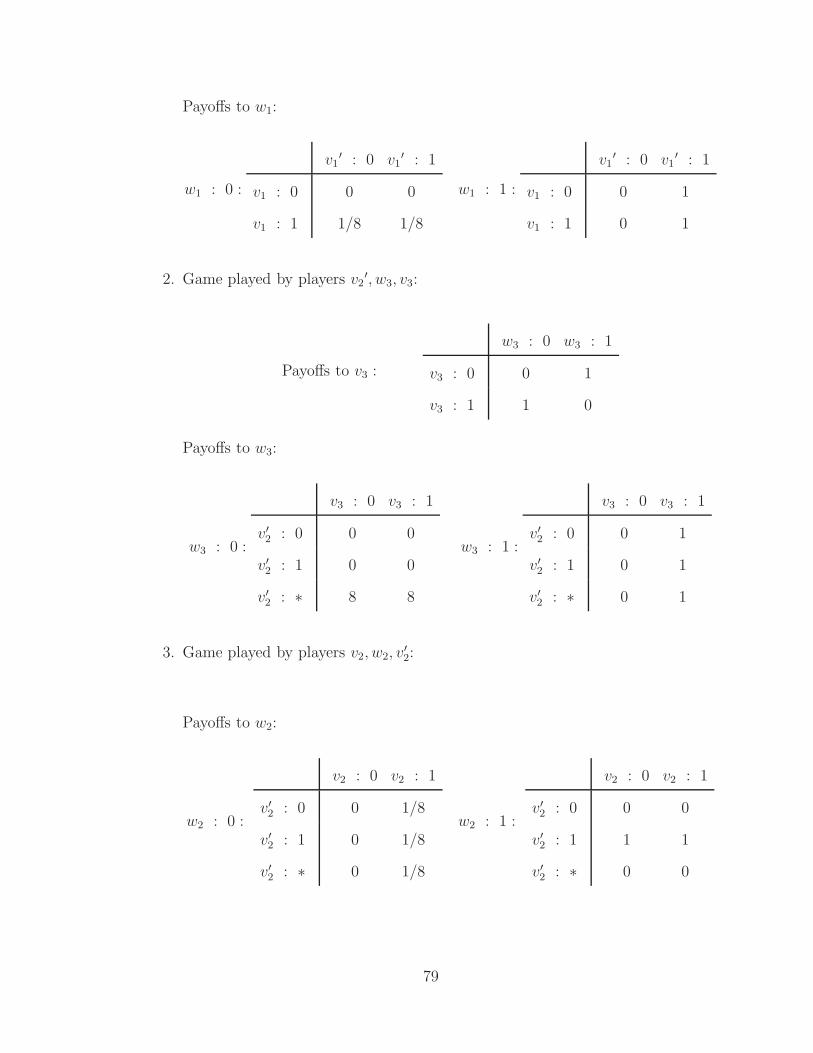
Payoffs to w1:
w1 : 0 :
v1′ : 0 v1
′ : 1
v1 : 0 0 0
v1 : 1 1/8 1/8
w1 : 1 :
v1′ : 0 v1
′ : 1
v1 : 0 0 1
v1 : 1 0 1
2. Game played by players v2′, w3, v3:
Payoffs to v3 :
w3 : 0 w3 : 1
v3 : 0 0 1
v3 : 1 1 0
Payoffs to w3:
w3 : 0 :
v3 : 0 v3 : 1
v′2 : 0 0 0
v′2 : 1 0 0
v′2 : ∗ 8 8
w3 : 1 :
v3 : 0 v3 : 1
v′2 : 0 0 1
v′2 : 1 0 1
v′2 : ∗ 0 1
3. Game played by players v2, w2, v′2:
Payoffs to w2:
w2 : 0 :
v2 : 0 v2 : 1
v′2 : 0 0 1/8
v′2 : 1 0 1/8
v′2 : ∗ 0 1/8
w2 : 1 :
v2 : 0 v2 : 1
v′2 : 0 0 0
v′2 : 1 1 1
v′2 : ∗ 0 0
79
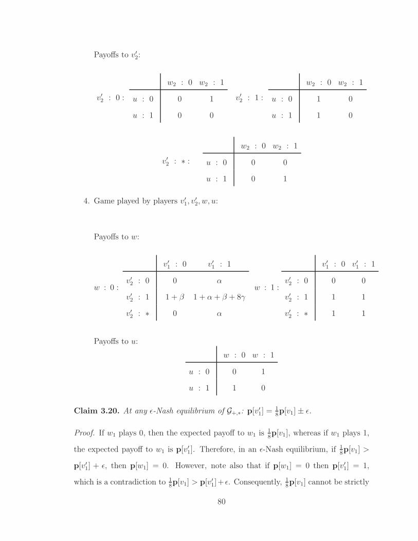
Payoffs to v′2:
v′2 : 0 :
w2 : 0 w2 : 1
u : 0 0 1
u : 1 0 0
v′2 : 1 :
w2 : 0 w2 : 1
u : 0 1 0
u : 1 1 0
v′2 : ∗ :
w2 : 0 w2 : 1
u : 0 0 0
u : 1 0 1
4. Game played by players v′1, v
′2, w, u:
Payoffs to w:
w : 0 :
v′1 : 0 v′
1 : 1
v′2 : 0 0 α
v′2 : 1 1 + β 1 + α + β + 8γ
v′2 : ∗ 0 α
w : 1 :
v′1 : 0 v′
1 : 1
v′2 : 0 0 0
v′2 : 1 1 1
v′2 : ∗ 1 1
Payoffs to u:
w : 0 w : 1
u : 0 0 1
u : 1 1 0
Claim 3.20. At any ǫ-Nash equilibrium of G+,∗: p[v′1] = 1
8p[v1] ± ǫ.
Proof. If w1 plays 0, then the expected payoff to w1 is 18p[v1], whereas if w1 plays 1,
the expected payoff to w1 is p[v′1]. Therefore, in an ǫ-Nash equilibrium, if 1
8p[v1] >
p[v′1] + ǫ, then p[w1] = 0. However, note also that if p[w1] = 0 then p[v′
1] = 1,
which is a contradiction to 18p[v1] > p[v′
1]+ ǫ. Consequently, 18p[v1] cannot be strictly
80
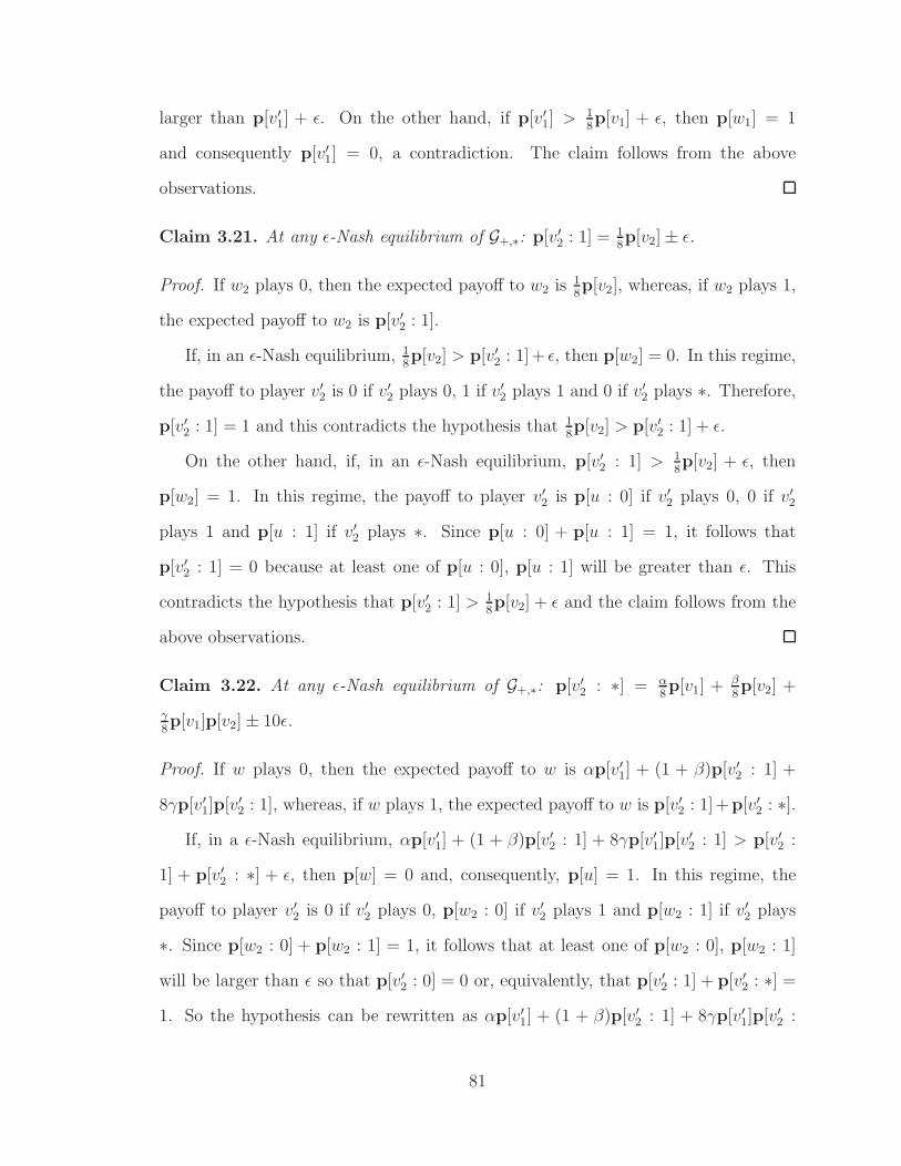
larger than p[v′1] + ǫ. On the other hand, if p[v′
1] > 18p[v1] + ǫ, then p[w1] = 1
and consequently p[v′1] = 0, a contradiction. The claim follows from the above
observations.
Claim 3.21. At any ǫ-Nash equilibrium of G+,∗: p[v′2 : 1] = 1
8p[v2] ± ǫ.
Proof. If w2 plays 0, then the expected payoff to w2 is 18p[v2], whereas, if w2 plays 1,
the expected payoff to w2 is p[v′2 : 1].
If, in an ǫ-Nash equilibrium, 18p[v2] > p[v′
2 : 1] + ǫ, then p[w2] = 0. In this regime,
the payoff to player v′2 is 0 if v′
2 plays 0, 1 if v′2 plays 1 and 0 if v′
2 plays ∗. Therefore,
p[v′2 : 1] = 1 and this contradicts the hypothesis that 1
8p[v2] > p[v′
2 : 1] + ǫ.
On the other hand, if, in an ǫ-Nash equilibrium, p[v′2 : 1] > 1
8p[v2] + ǫ, then
p[w2] = 1. In this regime, the payoff to player v′2 is p[u : 0] if v′
2 plays 0, 0 if v′2
plays 1 and p[u : 1] if v′2 plays ∗. Since p[u : 0] + p[u : 1] = 1, it follows that
p[v′2 : 1] = 0 because at least one of p[u : 0], p[u : 1] will be greater than ǫ. This
contradicts the hypothesis that p[v′2 : 1] > 1
8p[v2] + ǫ and the claim follows from the
above observations.
Claim 3.22. At any ǫ-Nash equilibrium of G+,∗: p[v′2 : ∗] = α
8p[v1] + β
8p[v2] +
γ8p[v1]p[v2] ± 10ǫ.
Proof. If w plays 0, then the expected payoff to w is αp[v′1] + (1 + β)p[v′
2 : 1] +
8γp[v′1]p[v′
2 : 1], whereas, if w plays 1, the expected payoff to w is p[v′2 : 1] +p[v′
2 : ∗].
If, in a ǫ-Nash equilibrium, αp[v′1] + (1 + β)p[v′
2 : 1] + 8γp[v′1]p[v′
2 : 1] > p[v′2 :
1] + p[v′2 : ∗] + ǫ, then p[w] = 0 and, consequently, p[u] = 1. In this regime, the
payoff to player v′2 is 0 if v′
2 plays 0, p[w2 : 0] if v′2 plays 1 and p[w2 : 1] if v′
2 plays
∗. Since p[w2 : 0] + p[w2 : 1] = 1, it follows that at least one of p[w2 : 0], p[w2 : 1]
will be larger than ǫ so that p[v′2 : 0] = 0 or, equivalently, that p[v′
2 : 1] + p[v′2 : ∗] =
1. So the hypothesis can be rewritten as αp[v′1] + (1 + β)p[v′
2 : 1] + 8γp[v′1]p[v′
2 :
81
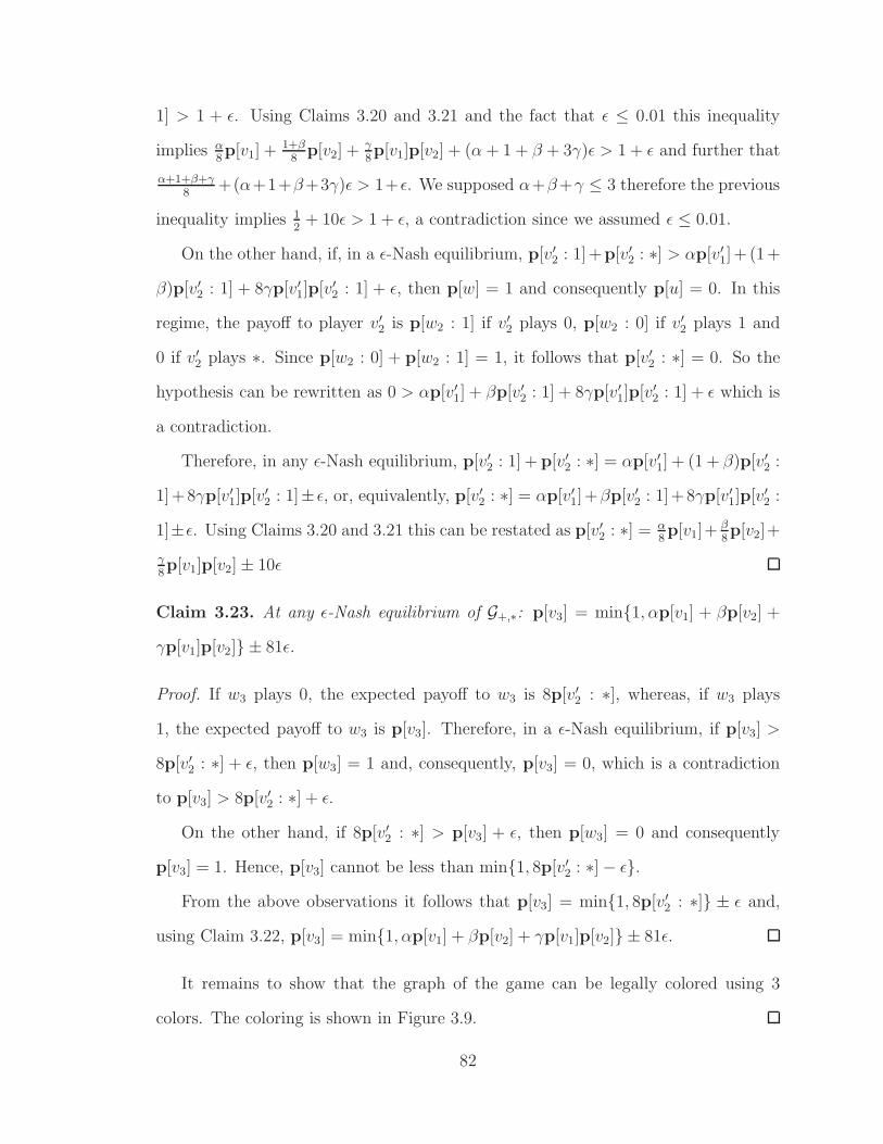
1] > 1 + ǫ. Using Claims 3.20 and 3.21 and the fact that ǫ ≤ 0.01 this inequality
implies α8p[v1] + 1+β
8p[v2] + γ
8p[v1]p[v2] + (α + 1 + β + 3γ)ǫ > 1 + ǫ and further that
α+1+β+γ8
+(α+1+β +3γ)ǫ > 1+ǫ. We supposed α+β +γ ≤ 3 therefore the previous
inequality implies 12
+ 10ǫ > 1 + ǫ, a contradiction since we assumed ǫ ≤ 0.01.
On the other hand, if, in a ǫ-Nash equilibrium, p[v′2 : 1] +p[v′
2 : ∗] > αp[v′1] + (1 +
β)p[v′2 : 1] + 8γp[v′
1]p[v′2 : 1] + ǫ, then p[w] = 1 and consequently p[u] = 0. In this
regime, the payoff to player v′2 is p[w2 : 1] if v′
2 plays 0, p[w2 : 0] if v′2 plays 1 and
0 if v′2 plays ∗. Since p[w2 : 0] + p[w2 : 1] = 1, it follows that p[v′
2 : ∗] = 0. So the
hypothesis can be rewritten as 0 > αp[v′1] + βp[v′
2 : 1] + 8γp[v′1]p[v′
2 : 1] + ǫ which is
a contradiction.
Therefore, in any ǫ-Nash equilibrium, p[v′2 : 1] + p[v′
2 : ∗] = αp[v′1] + (1 + β)p[v′
2 :
1] + 8γp[v′1]p[v′
2 : 1]± ǫ, or, equivalently, p[v′2 : ∗] = αp[v′
1] +βp[v′2 : 1] + 8γp[v′
1]p[v′2 :
1]±ǫ. Using Claims 3.20 and 3.21 this can be restated as p[v′2 : ∗] = α
8p[v1]+ β
8p[v2]+
γ8p[v1]p[v2] ± 10ǫ
Claim 3.23. At any ǫ-Nash equilibrium of G+,∗: p[v3] = min1, αp[v1] + βp[v2] +
γp[v1]p[v2] ± 81ǫ.
Proof. If w3 plays 0, the expected payoff to w3 is 8p[v′2 : ∗], whereas, if w3 plays
1, the expected payoff to w3 is p[v3]. Therefore, in a ǫ-Nash equilibrium, if p[v3] >
8p[v′2 : ∗] + ǫ, then p[w3] = 1 and, consequently, p[v3] = 0, which is a contradiction
to p[v3] > 8p[v′2 : ∗] + ǫ.
On the other hand, if 8p[v′2 : ∗] > p[v3] + ǫ, then p[w3] = 0 and consequently
p[v3] = 1. Hence, p[v3] cannot be less than min1, 8p[v′2 : ∗] − ǫ.
From the above observations it follows that p[v3] = min1, 8p[v′2 : ∗] ± ǫ and,
using Claim 3.22, p[v3] = min1, αp[v1] + βp[v2] + γp[v1]p[v2] ± 81ǫ.
It remains to show that the graph of the game can be legally colored using 3
colors. The coloring is shown in Figure 3.9.
82
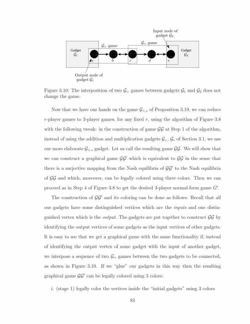
Gadget Gadget
G1
a b c d e
G2
Input node of
Output node of
gadget G2
gadget G1
G= gameG= game
Figure 3.10: The interposition of two G= games between gadgets G1 and G2 does notchange the game.
Now that we have our hands on the game G+,∗ of Proposition 3.19, we can reduce
r-player games to 3-player games, for any fixed r, using the algorithm of Figure 3.8
with the following tweak: in the construction of game GG at Step 1 of the algorithm,
instead of using the addition and multiplication gadgets G+, G∗ of Section 3.1, we use
our more elaborate G+,∗ gadget. Let us call the resulting game GG. We will show that
we can construct a graphical game GG′ which is equivalent to GG in the sense that
there is a surjective mapping from the Nash equilibria of GG′ to the Nash equilibria
of GG and which, moreover, can be legally colored using three colors. Then we can
proceed as in Step 4 of Figure 3.8 to get the desired 3-player normal-form game G′.
The construction of GG′ and its coloring can be done as follows: Recall that all
our gadgets have some distinguished vertices which are the inputs and one distin-
guished vertex which is the output. The gadgets are put together to construct GG by
identifying the output vertices of some gadgets as the input vertices of other gadgets.
It is easy to see that we get a graphical game with the same functionality if, instead
of identifying the output vertex of some gadget with the input of another gadget,
we interpose a sequence of two G= games between the two gadgets to be connected,
as shown in Figure 3.10. If we “glue” our gadgets in this way then the resulting
graphical game GG ′ can be legally colored using 3 colors:
i. (stage 1) legally color the vertices inside the “initial gadgets” using 3 colors
83
ii. (stage 2) extend the coloring to the vertices that serve as “connections” between
gadgets; any 3-coloring of the initial gadgets can be extended to a 3-coloring of
GG′ because, for any pair of gadgets G1, G2 which are connected (Figure 3.10)
and for any colors assigned to the output vertex a of gadget G1 and the input
vertex e of gadget G2, the intermediate vertices b, c and d can be also colored
legally. For example, if vertex a gets color 1 and vertex e color 2 at stage 1,
then, at stage 2, b can be colored 2, c can be colored 3 and d can be colored 1.
This completes the proof of the theorem.
3.6 Preservation of Approximate equilibria
Our reductions so far map exact equilibrium points. In this section we generalize
to approximate equilibria and prove the second part of Theorem 3.1. We claim
that the reductions of the previous sections translate the problem of finding an ǫ-
Nash equilibrium of a game to the problem of finding an ǫ′-Nash equilibrium of its
image, for ǫ′ polynomial in ǫ and inverse polynomial in the size of the game. As
a consequence, we obtain polynomial-time equivalence results for the problems r-
Nash and d-graphical-Nash. To prove the second part of Theorem 3.1, we extend
Theorems 3.8, 3.12 and 3.18 of the previous sections.
Theorem 3.24. For every fixed d > 1, there is a polynomial-time reduction from
d-graphical-Nash to (d2 + 1)-Nash.
Proof. Let GG be a graphical game of maximum degree d and GG the resulting graph-
ical game after rescaling all utilities by 1/ max u, where max u is the largest entry
in the utility tables of game GG, so that they lie in the set [0, 1], as in the first step of
Figure 3.5. Assume that ǫ < 1. In time polynomial in |GG|+ log(1/ǫ), we will specify
a normal-form game G and an accuracy ǫ′ with the property that, given an ǫ′-Nash
84
equilibrium of G, one can recover in polynomial time an ǫ-Nash equilibrium of GG.
This will be enough, since an ǫ-Nash equilibrium of GG is trivially an ǫ ·max u-Nash
equilibrium of game GG and, moreover, |GG| is polynomial in |GG|.
We construct G using the algorithm of Figure 3.5; recall that M ≥ 2nr, where r
is the number of color classes specified in Figure 3.5 and n is the number of vertices
in GG after the possible addition of dummy vertices to make sure that all color
classes have the same number of vertices (as in Step 3 of Figure 3.5). Let us choose
ǫ′ ≤ ǫ( rn− 1
M)d; we will argue that from any ǫ′-Nash equilibrium of game G one can
construct in polynomial time an ǫ-Nash equilibrium of game GG.
Suppose that p = c(v) for some vertex v of the graphical game GG. As in the
proof of Theorem 3.8, Lemma 3.11, it can be shown that in any ǫ′-Nash equilibrium
of the game G,
Pr[p plays v] ∈[
r
n− 1
M,r
n+
1
M
].
Now, without loss of generality, assume that p is odd (pursuer) and suppose that v is
vertex v(p)i in the notation of Figure 3.5. Then, in an ǫ′-Nash equilibrium of the game
G, we have, by the definition of a Nash equilibrium, that for all strategies a, a′ ∈ Sv
of vertex v:
E [payoff to p for playing (v, a)] > E [payoff to p for playing (v, a′)] + ǫ′ ⇒ xp(v,a′) = 0.
But
E [payoff to p for playing (v, a)]
= M · Pr[p + 1 plays v
(p+1)i
]+
∑
s∈SN (v)\v
uvas
∏
u∈N (v)\vx
c(u)(u,su)
85
and, similarly, for a′. Therefore, the previous inequality implies
∑
s∈SN (v)\v
uvas
∏
u∈N (v)\vx
c(u)(u,su) >
∑
s∈SN (v)\v
uva′s
∏
u∈N (v)\vx
c(u)(u,su) + ǫ′ ⇒ xp
(v,a′) = 0
So letting
xva = x
c(v)(v,a)
/∑
j∈Sv
xc(v)(v,j), ∀v ∈ V, a ∈ Sv,
as we did in the proof of Theorem 3.8, we get that, for all v ∈ V , a, a′ ∈ Sv,
∑
s∈SN (v)\v
uvas
∏
u∈N (v)\vxu
su>
∑
s∈SN (v)\v
uva′s
∏
u∈N (v)\vxu
su+ ǫ′/T ⇒ xv
a′ = 0, (3.5)
where T =∏
u∈N (v)\v∑
j∈Sux
c(u)(u,j) =
∏u∈N (v)\v Pr[c(u) plays u] ≥ ( r
n− 1
M)d. By
the definition of ǫ′ it follows that ǫ′/T ≤ ǫ. Hence, from (3.5) it follows that xvav,a
is an ǫ-Nash equilibrium of the game GG.
We have the following extension of Theorem 3.12.
Theorem 3.25. For every fixed r > 1, there is a polynomial-time reduction from
r-Nash to 3-graphical Nash with two strategies per vertex.
Proof. Let G be a normal-form game with r players, 1, 2, . . . , r, and strategy sets
Sp = [n], for all p ∈ [r], and let ups : p ∈ [r], s ∈ S be the utilities of the players.
Denote by G the game constructed at the first step of Figure 3.7 which results from G
after rescaling all utilities by 1/ max ups so that they lie in [0, 1]; let up
s : p ∈ [r], s ∈
S be the utilities of the players in game G. Also, let ǫ < 1. In time polynomial
in |G| + log(1/ǫ), we will specify a graphical game GG and an accuracy ǫ′ with the
property that, given an ǫ′-Nash equilibrium of GG, one can recover in polynomial time
an ǫ-Nash equilibrium of G. This will be enough, since an ǫ-Nash equilibrium of G is
86

trivially an ǫ ·max ups-Nash equilibrium of game G and, moreover, |G| is polynomial
in |G|. In our reduction, the graphical game GG will be the same as the one described
in the proof of Theorem 3.12 (Figure 3.7), while the accuracy specification will be of
the form ǫ′ = ǫ/p(|G|), where p(·) is a polynomial that will be be specified later. We
will use the same labels for the vertices of the game GG that we used in the proof
Theorem 3.12.
Suppose NGG is some ǫ′-Nash equilibrium of the game GG and let p[v(xpj )]j,p
denote the probabilities with which the vertices v(xpj ) of GG play strategy 1. In the
proof of Theorem 3.12 we considered the following mapping from the Nash equilibria
of game GG to the Nash equilibria of game G:
xpj := p[v(xp
j )], for all p and j. (3.6)
Although (3.6) succeeds in mapping exact equilibrium points, it fails for approximate
equilibria, as specified by the following remark —its justification follows from the
proof of Lemma 3.27.
Remark 3.26. For any ǫ′ > 0, there exists an ǫ′-Nash equilibrium of game GG such
that∑
j p[v(xpj )] 6= 1, for some player p ≤ r, and, moreover, p[v(Up
j )] > p[v(Upj′)]+ǫ′,
for some p ≤ r, j and j′, and, yet, p[v(xpj′)] > 0.
Recall from Section 3.3, that, for all p, j, the probability p[v(Upj )] represents the
utility of player p for playing pure strategy j, when the other players play according to
xqj := p[v(xq
j)]j,q 6=p.3 Therefore, not only the xp
j := p[v(xpj )]j do not necessarily
constitute a distribution —this could be easily fixed by rescaling— but, also, the
defining property of an approximate equilibrium (2.2) is in question. The following
lemma bounds the deviation from the approximate equilibrium conditions.
3Note, however, that, since we are considering an ǫ′-Nash equilibrium of game GG, Equation (3.3)of Section 3.3 will be only satisfied approximately as specified by Lemma 3.29.
87

Lemma 3.27. In any ǫ′-Nash equilibrium of the game GG,
(i) for all p ∈ [r], |∑j p[v(xpj )] − 1| ≤ 2cnǫ′, and,
(ii) for all p ∈ [r], j, j′ ∈ [n], p[v(Upj )] > p[v(Up
j′)] + 5cnǫ′ ⇒ p[v(xpj′)] ∈ [0, cnǫ′],
where c ≥ 1 is the maximum error amplification of the gadgets used in the construction
of GG.
Proof. Note that at an ǫ′-Nash equilibrium of game GG the following properties are
satisfied for all p ∈ [r] by the vertices of game GG, since the error amplification of the
gadgets is at most c:
p
[v
(n∑
i=1
xpi
)]= 1 (3.7)
p
[v
(j∑
i=1
xpi
)]= p
[v
(j+1∑
i=1
xpi
)]· (1 − p[vp
j ]) ± cǫ′, ∀j < n (3.8)
p[v(xp
j+1)]
= p
[v
(j+1∑
i=1
xpi
)]· p[vp
j ] ± cǫ′, ∀j < n (3.9)
p [v(xp1)] = p
[v
(1∑
i=1
xpi
)]± cǫ′ (3.10)
88
Proof of (i): By successive applications of (3.8) and (3.9), we deduce
n∑
j=1
p[v(xpj )] =
n∑
j=2
p
[v
(j∑
i=1
xpi
)]· p[vp
j−1]
+ p
[v
(1∑
i=1
xpi
)]± cnǫ′
=n∑
j=2
p
[v
(j∑
i=1
xpi
)]· p[vp
j−1]
+
(p
[v
(2∑
i=1
xpi
)]· (1 − p[vp
1 ]) ± cǫ′)
± cnǫ′
=
n∑
j=3
p
[v
(j∑
i=1
xpi
)]· p[vp
j−1]
+ p
[v
(2∑
i=1
xpi
)]± c(n + 1)ǫ′
= . . .
= p
[v
(n∑
i=1
xpi
)]± c(2n − 1)ǫ′
= 1 ± c(2n − 1)ǫ′
Proof of (ii): Let us first observe the behavior of vertices w(Upj ) and vp
j in an ǫ′-Nash
equilibrium.
• Behavior of w(Upj ) vertices: The utility of vertex w(Up
j ) for playing strategy
0 is p[v(Up≤j)], whereas for playing 1 it is p[v(Up
j+1)]. Therefore,
p[v(Up≤j)] > p[v(Up
j+1)] + ǫ′ ⇒ p[w(Upj )] = 0
p[v(Upj+1)] > p[v(Up
≤j)] + ǫ′ ⇒ p[w(Upj )] = 1
|p[v(Upj+1)] − p[v(Up
≤j)]| ≤ ǫ′ ⇒ p[w(Upj )] can be anything
• Behavior of vpj vertices: The utility of vertex vp
j for playing strategy 0 is
1 − p[w(Upj )], whereas for playing 1 it is p[w(Up
j )]. Therefore,
p[w(Upj )] < 1−ǫ′
2⇒ p[vp
j ] = 0
p[w(Upj )] > 1+ǫ′
2⇒ p[vp
j ] = 1
|p[w(Upj )] − 1
2| ≤ ǫ′
2⇒ p[vp
j ] can be anything
89
Note that, since the error amplification of the gadget Gmax is at most c and computing
p[v(Up≤j)], for all j, requires j applications of Gmax,
p[v(Up≤j)] = max
i≤jp[v(Up
i )] ± cǫ′j. (3.11)
To establish the second part of the claim, we need to show that, for all p, j, j′,
p[v(Upj )] > p[v(Up
j′)] + 5cnǫ′ ⇒ p[v(xpj′)] ∈ [0, ncǫ′].
1. Note that, if there exists some j′′ < j′ such that p[v(Upj′′)] > p[v(Up
j′)] + cǫ′n,
then
p[v(Up≤j′−1)] = max
i≤j′−1p[v(Up
i )] ± cǫ′(j′ − 1)
≥ p[v(Upj′′)] − cǫ′(j′ − 1)
> p[v(Upj′)] + cnǫ′ − cǫ′(j′ − 1) ≥ p[v(Up
j′)] + ǫ′.
Then, because p[v(Up≤j′−1)] > p[v(Up
j′)] + ǫ′, it follows that p[w(Upj′−1)] = 0 and
p[vpj′−1] = 0. Therefore,
p[v(xpj′)] = p
[v
(j′∑
i=1
xpi
)]· p[vp
j′−1] ± cǫ′ = ±cǫ′.
2. The case j < j′ reduces to the previous for j′′ = j.
3. It remains to deal with the case j > j′, under the assumption that, for all
j′′ < j′,
p[v(Upj′′)] ≤ p[v(Up
j′)] + cǫ′n.
90
which, in turn, implies
p[v(Up≤j′)] < p[v(Up
j′)] + 2cǫ′n. (by (3.11))
Let us further distinguish the following subcases
(a) If there exists some k, j′+1 ≤ k ≤ j, such that p[v(Upk )] > p[v(Up
≤k−1)]+ǫ′,
then
p[w(Upk−1)] = 1 ⇒ p[vp
k−1] = 1
⇒ p
[v
(k−1∑
i=1
xpi
)]= p
[v
(k∑
i=1
xpi
)](1 − p[vp
k−1]) ± cǫ′ = ±cǫ′
⇒ p
[v
(j′∑
i=1
xpi
)]= ±(k − j′)cǫ′
(by successive applications
of equation (3.8)
)
⇒ p[v(xp
j′)]
= ±ncǫ′. (by (3.9), (3.10))
(b) If, for all k, j′ + 1 ≤ k ≤ j, it holds that p[v(Upk )] ≤ p[v(Up
≤k−1)] + ǫ′, we
will show a contradiction; hence, only the previous case can hold. Towards
a contradiction,we argue first that
p[v(Up≤j′+1)] ≥ p[v(Up
j )] − 2cnǫ′.
To show this, we distinguish the cases j = j′ + 1, j > j′ + 1.
• In the case j = j′ + 1, we have
p[v(Up≤j′+1)] ≥ max p[v(Up
j′+1)],p[v(Up≤j′)] − cǫ′
≥ p[v(Upj′+1)] − cǫ′ = p[v(Up
j )] − cǫ′.
91
• In the case j > j′ + 1, we have for all k, j′ + 2 ≤ k ≤ j,
p[v(Up≤k−1)] ≥ max p[v(Up
≤k−1)],p[v(Upk )]− ǫ′ ≥ p[v(Up
≤k)]− cǫ′ − ǫ′,
where the last inequality holds since the game Gmax has error amplifi-
cation at most c. Summing these inequalities for j′ + 2 ≤ k ≤ j, we
deduce that
p[v(Up≤j′+1)] ≥ p[v(Up
≤j)] − (cǫ′ + ǫ′)(n − 2)
≥ max p[v(Upj )],p[v(Up
≤j−1)] − cǫ′ − (cǫ′ + ǫ′)(n − 2)
≥ p[v(Upj )] − 2cǫ′n.
It follows that
p[v(Up≤j′+1)] > p[v(Up
j′)] + 3cnǫ′.
But,
p[v(Up≤j′+1)] ≤ max p[v(Up
j′+1)],p[v(Up≤j′)] + cǫ′
and recall that
p[v(Up≤j′)] < p[v(Up
j′)] + 2cǫ′n.
We can deduce that
max p[v(Upj′+1)],p[v(Up
≤j′)] = p[v(Upj′+1)],
which combined with the above implies
p[v(Upj′+1)] ≥ p[v(Up
j′)] + 3cnǫ′ − cǫ′ > p[v(Up≤j′)] + ǫ′.
92
From Lemma 3.27, it follows that the extraction of an ǫ-Nash equilibrium of game
G from an ǫ′-Nash equilibrium of game GG cannot be done by just interpreting the
values xpj := p[v(xp
j )]j as the mixed strategy of player p. What we show next is
that, for the right choice of ǫ′, a trim and renormalize transformation succeeds in
deriving an ǫ-Nash equilibrium of game G from an ǫ′-Nash equilibrium of game GG.
Indeed, for all p ≤ r, suppose that xpjj are the values derived from xp
jj by setting
xpj =
0, if xpj ≤ cnǫ′
xpj , otherwise
and then renormalizing the resulting values xpjj so that
∑j xp
j = 1.
Lemma 3.28. There exists a polynomial p(·) such that, if xpjjp is an ǫ/p(|G|)-
Nash equilibrium of game GG, then the trimmed and renormalized values xpjjp
constitute an ǫ-Nash equilibrium of game G.
Proof. We first establish the following useful lemma
Lemma 3.29. At an ǫ′-Nash equilibrium of game GG, for all p, j, it holds that
p[v(Upj )] =
∑
s∈S−p
upjsx
1s1· · ·xp−1
sp−1xp+1
sp+1· · ·xr
sr± 2nr−1ζr,
where c is the maximum error amplification of the gadgets used in the construction of
GG, ζr = cǫ′ + ((1 + ζ)r − 1)(cǫ′ + 1), ζ = 2r log n cǫ′.
Proof. Using the same notation as in Section 3.3, let S−p = S−p(1), . . . , S−p(nr−1),
so that∑
s∈S−p
upjsxs =
nr−1∑
ℓ=1
upjS−p(ℓ)xS−p(ℓ).
93
Recall that in GG, for each partial sum∑z
ℓ=1 upjS−p(ℓ)xS−p(ℓ), 1 ≤ z ≤ nr−1, we have
included vertex v(∑z
ℓ=1 upjS−p(ℓ)xS−p(ℓ)). Similarly, for each partial product of the
summands upjs
∏p 6=q≤z xq
sq, 0 ≤ z ≤ r, we have included vertex v(up
js
∏p 6=q≤z xq
sq).
Note that, since we have rescaled the utilities to the set [0, 1], all partial sums and
products must also lie in [0, 1]. Note, moreover, that, to avoid large degrees in the
resulting graphical game, each time we need to make use of a value xqsq
we create a
new copy of the vertex v(xqsq
) using the gadget G= and, then, use the new copy for the
computation of the desired partial product; an easy calculation shows that we have
to make (r−1)nr−1 copies of v(xqsq
), for all q ≤ r, sq ∈ Sq. To limit the degree of each
vertex to 3 we create a binary tree of copies of v(xqsq
) with (r − 1)nr−1 leaves and use
each leaf once. Then, because of the error amplification of G=, this already induces
an error of ±⌈log (r − 1)nr−1⌉cǫ′ to each of the factors of the partial products. The
following lemma characterizes the error that results from the error amplification of
our gadgets in the computation of the partial products and can be proved easily by
induction.
Lemma 3.30. For all p ≤ r, j ∈ Sp, s ∈ S−p and z ≤ r,
p
[v
(up
js
∏
p 6=ℓ≤z
xℓsℓ
)]= up
js
∏
p 6=ℓ≤z
xℓsℓ± ζz, (3.12)
where ζz = cǫ′ + ((1 + ζ)z − 1)(cǫ′ + 1), ζ = 2r log n cǫ′.
The following lemma characterizes the error in the computation of the partial
sums and can be proved by induction using the previous lemma for the base case.
Lemma 3.31. For all p ≤ r, j ∈ Sp and z ≤ nr−1,
p
[v
(z∑
ℓ=1
upjS−p(ℓ)xS−p(ℓ)
)]=
z∑
ℓ=1
upjS−p(ℓ)xS−p(ℓ) ± (zζr + (z − 1)cǫ′), (3.13)
94
where ζr is defined as in Lemma 3.30.
From Lemma 3.31 we can deduce, in particular, that for all p ≤ r, j ∈ Sp,
p[v(Upj )] =
∑
s∈S−p
upjsxs ± 2nr−1ζr.
Lemma 3.32. For all p ≤ r, j ∈ Sp,
∣∣∣∣∣∣
∑
s∈S−p
upjsxs −
∑
s∈S−p
upjsys
∣∣∣∣∣∣≤ max
s∈S−p
upjs∑
q 6=p
∑
i∈Sq
|xqi − yq
i |.
Proof. We have
∣∣∣∣∣∣
∑
s∈S−p
upjsxs −
∑
s∈S−p
upjsys
∣∣∣∣∣∣≤∑
s∈S−p
upjs |xs − ys| ≤ max
s∈S−p
upjs
∑
s∈S−p
|xs − ys| . (3.14)
Let us denote by X q the random variable, ranging over the set Sq, which represents
the mixed strategy xqii∈Sq , q ≤ r. Similarly, define the random variable Yq from the
mixed strategy yqi i∈Sq , q ≤ r. Note, then, that 1
2
∑s∈S−p
|xs − ys| is precisely the
total variation distance between the vector random variable (X q)q 6=p and the vector
random variable (Yq)q 6=p. That is,
1
2
∑
s∈S−p
|xs − ys| = ||(X q)q 6=p − (Yq)q 6=p||TV . (3.15)
By the coupling lemma, we have that
||(X q)q 6=p − (Yq)q 6=p||TV ≤ Pr [(X q)q 6=p 6= (Yq)q 6=p] ,
for any coupling of (X q)q 6=p and (Yq)q 6=p. Applying a union bound to the right hand
95

side of the above implies
||(X q)q 6=p − (Yq)q 6=p||TV ≤∑
q 6=p
Pr [X q 6= Yq] . (3.16)
Now let us fix a coupling between (X q)q 6=p and (Yq)q 6=p so that, for all q 6= p,
Pr [X q 6= Yq] = ||X q − Yq||TV .
Such a coupling exists by the coupling lemma for each q 6= p individually, and for the
whole vectors (X q)q 6=p and (Yq)q 6=p it exists because also the X q’s are independent
and so are the Yq’s. Then (3.16) implies that
||(X q)q 6=p − (Yq)q 6=p||TV ≤∑
q 6=p
||X q −Yq||TV ,
so that from (3.14), (3.15) we get
∣∣∣∣∣∣
∑
s∈S−p
upjsxs −
∑
s∈S−p
upjsys
∣∣∣∣∣∣≤ max
s∈S−p
upjs2
∑
q 6=p
||X q −Yq||TV . (3.17)
Now, note that, for all q,
||X q −Yq||TV =1
2
∑
i∈Sq
|xqi − yq
i |.
Hence, (3.17) implies
∣∣∣∣∣∣
∑
s∈S−p
upjsxs −
∑
s∈S−p
upjsys
∣∣∣∣∣∣≤ max
s∈S−p
upjs∑
q 6=p
∑
i∈Sq
|xqi − yq
i |.
96
We can conclude the proof of Lemma 3.28, by invoking Lemmas 3.29 and 3.32.
Indeed, by the definition of the xpj, it follows that for all p, j ∈ Sp,
xpj =
xpj
Λp , xpj > cnǫ′
0, xpj ≤ cnǫ′
,
where
1 ≥ Λp =∑
j∈Sp
xpjXxp
j >cnǫ′ = 1 −∑
j∈Sp
xpjXxp
j≤cnǫ′ ≥ 1 − n · cnǫ′,
where X· is the indicator function. Therefore,
|xpj − xp
j | =
xpj
Λp − xpj , xp
j > cnǫ′
xpj , xp
j ≤ cnǫ′,
which implies
|xpj − xp
j | ≤
1Λp − 1, xp
j > cnǫ′
cnǫ′, xpj ≤ cnǫ′
.
So,
|xpj − xp
j | ≤ max
cnǫ′,
n2cǫ′
1 − n2cǫ′
=: δ1,
which by Lemma 3.32 implies that
∣∣∣∣∣∣
∑
s∈S−p
upjsxs −
∑
s∈S−p
upjsxs
∣∣∣∣∣∣≤ max
s∈S−p
upjs(r − 1)nδ1 ≤ (r − 1)nδ1 =: δ2, (3.18)
where the second inequality follows from the fact that we have rescaled the utilities
so that they lie in [0, 1].
97
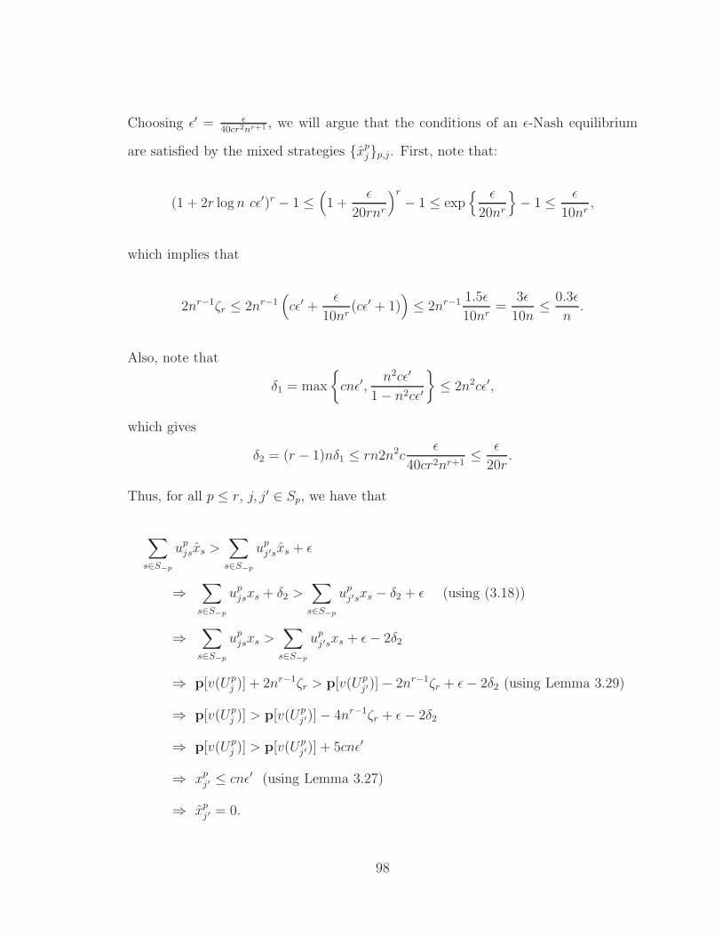
Choosing ǫ′ = ǫ40cr2nr+1 , we will argue that the conditions of an ǫ-Nash equilibrium
are satisfied by the mixed strategies xpjp,j. First, note that:
(1 + 2r log n cǫ′)r − 1 ≤(
1 +ǫ
20rnr
)r
− 1 ≤ exp ǫ
20nr
− 1 ≤ ǫ
10nr,
which implies that
2nr−1ζr ≤ 2nr−1(cǫ′ +
ǫ
10nr(cǫ′ + 1)
)≤ 2nr−1 1.5ǫ
10nr=
3ǫ
10n≤ 0.3ǫ
n.
Also, note that
δ1 = max
cnǫ′,
n2cǫ′
1 − n2cǫ′
≤ 2n2cǫ′,
which gives
δ2 = (r − 1)nδ1 ≤ rn2n2cǫ
40cr2nr+1≤ ǫ
20r.
Thus, for all p ≤ r, j, j′ ∈ Sp, we have that
∑
s∈S−p
upjsxs >
∑
s∈S−p
upj′sxs + ǫ
⇒∑
s∈S−p
upjsxs + δ2 >
∑
s∈S−p
upj′sxs − δ2 + ǫ (using (3.18))
⇒∑
s∈S−p
upjsxs >
∑
s∈S−p
upj′sxs + ǫ − 2δ2
⇒ p[v(Upj )] + 2nr−1ζr > p[v(Up
j′)] − 2nr−1ζr + ǫ − 2δ2 (using Lemma 3.29)
⇒ p[v(Upj )] > p[v(Up
j′)] − 4nr−1ζr + ǫ − 2δ2
⇒ p[v(Upj )] > p[v(Up
j′)] + 5cnǫ′
⇒ xpj′ ≤ cnǫ′ (using Lemma 3.27)
⇒ xpj′ = 0.
98
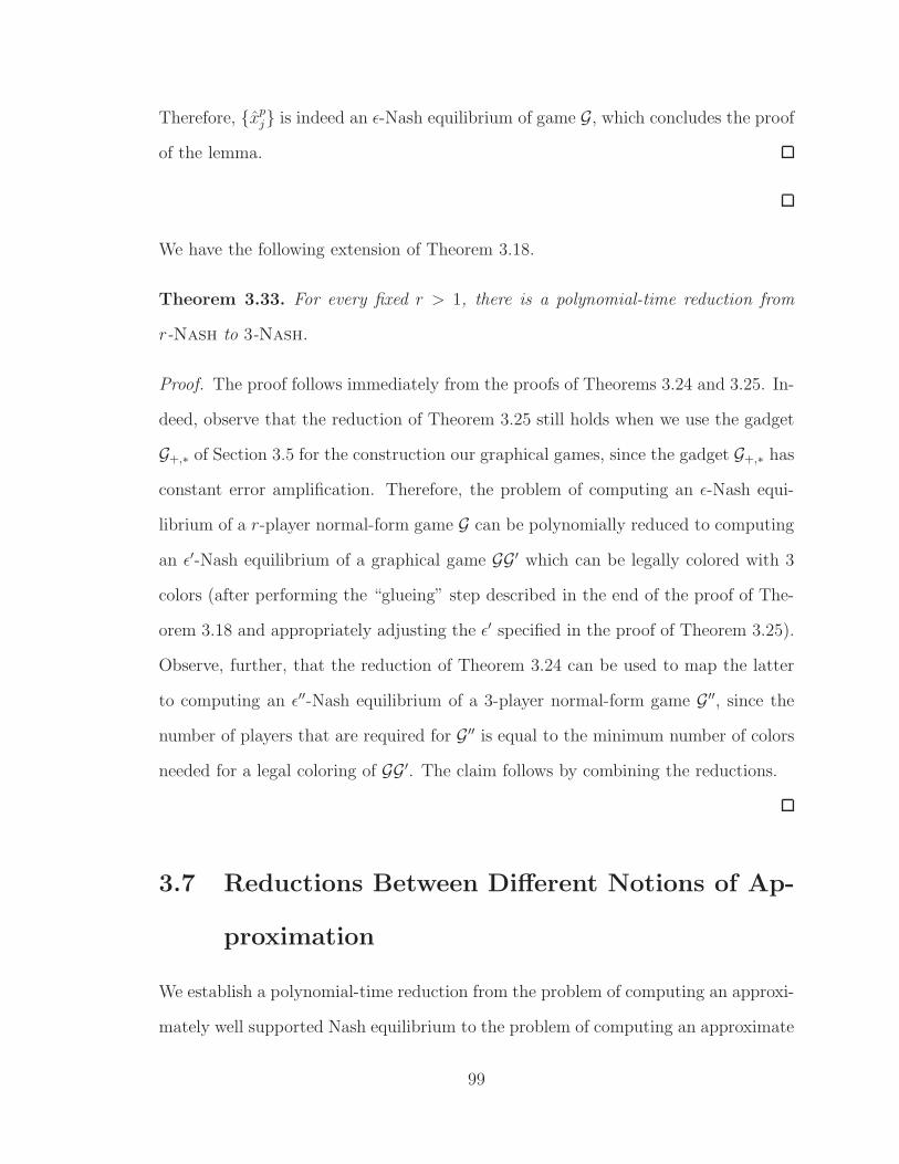
Therefore, xpj is indeed an ǫ-Nash equilibrium of game G, which concludes the proof
of the lemma.
We have the following extension of Theorem 3.18.
Theorem 3.33. For every fixed r > 1, there is a polynomial-time reduction from
r-Nash to 3-Nash.
Proof. The proof follows immediately from the proofs of Theorems 3.24 and 3.25. In-
deed, observe that the reduction of Theorem 3.25 still holds when we use the gadget
G+,∗ of Section 3.5 for the construction our graphical games, since the gadget G+,∗ has
constant error amplification. Therefore, the problem of computing an ǫ-Nash equi-
librium of a r-player normal-form game G can be polynomially reduced to computing
an ǫ′-Nash equilibrium of a graphical game GG′ which can be legally colored with 3
colors (after performing the “glueing” step described in the end of the proof of The-
orem 3.18 and appropriately adjusting the ǫ′ specified in the proof of Theorem 3.25).
Observe, further, that the reduction of Theorem 3.24 can be used to map the latter
to computing an ǫ′′-Nash equilibrium of a 3-player normal-form game G′′, since the
number of players that are required for G′′ is equal to the minimum number of colors
needed for a legal coloring of GG′. The claim follows by combining the reductions.
3.7 Reductions Between Different Notions of Ap-
proximation
We establish a polynomial-time reduction from the problem of computing an approxi-
mately well supported Nash equilibrium to the problem of computing an approximate
99
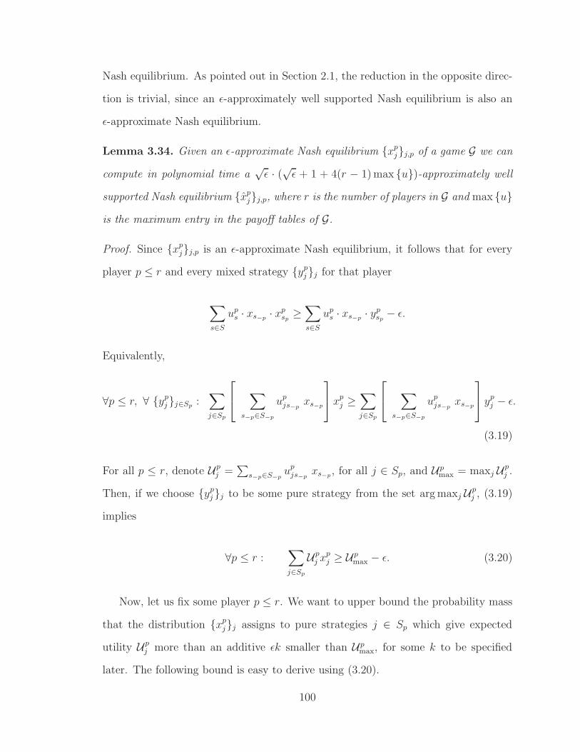
Nash equilibrium. As pointed out in Section 2.1, the reduction in the opposite direc-
tion is trivial, since an ǫ-approximately well supported Nash equilibrium is also an
ǫ-approximate Nash equilibrium.
Lemma 3.34. Given an ǫ-approximate Nash equilibrium xpjj,p of a game G we can
compute in polynomial time a√
ǫ · (√
ǫ + 1 + 4(r − 1) max u)-approximately well
supported Nash equilibrium xpjj,p, where r is the number of players in G and max u
is the maximum entry in the payoff tables of G.
Proof. Since xpjj,p is an ǫ-approximate Nash equilibrium, it follows that for every
player p ≤ r and every mixed strategy ypjj for that player
∑
s∈S
ups · xs−p · xp
sp≥∑
s∈S
ups · xs−p · yp
sp− ǫ.
Equivalently,
∀p ≤ r, ∀ ypjj∈Sp :
∑
j∈Sp
∑
s−p∈S−p
upjs−p
xs−p
xp
j ≥∑
j∈Sp
∑
s−p∈S−p
upjs−p
xs−p
yp
j − ǫ.
(3.19)
For all p ≤ r, denote Upj =
∑s−p∈S−p
upjs−p
xs−p, for all j ∈ Sp, and Upmax = maxj Up
j .
Then, if we choose ypjj to be some pure strategy from the set arg maxj Up
j , (3.19)
implies
∀p ≤ r :∑
j∈Sp
Upj xp
j ≥ Upmax − ǫ. (3.20)
Now, let us fix some player p ≤ r. We want to upper bound the probability mass
that the distribution xpjj assigns to pure strategies j ∈ Sp which give expected
utility Upj more than an additive ǫk smaller than Up
max, for some k to be specified
later. The following bound is easy to derive using (3.20).
100
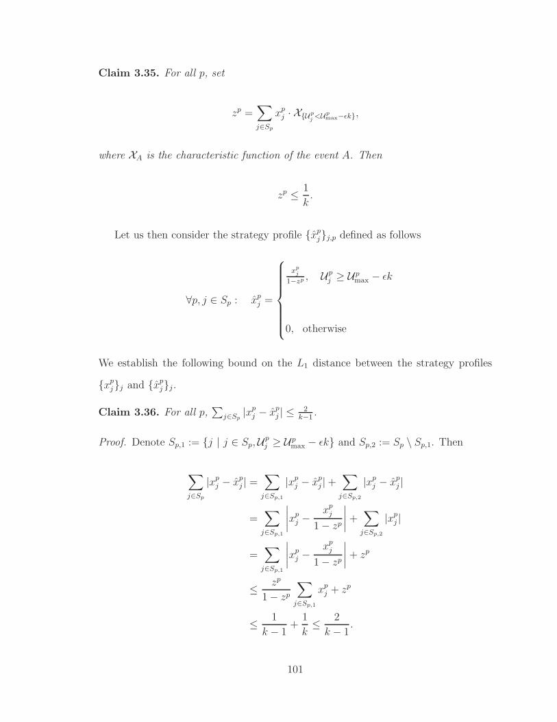
Claim 3.35. For all p, set
zp =∑
j∈Sp
xpj · XUp
j <Upmax−ǫk,
where XA is the characteristic function of the event A. Then
zp ≤ 1
k.
Let us then consider the strategy profile xpjj,p defined as follows
∀p, j ∈ Sp : xpj =
xpj
1−zp , Upj ≥ Up
max − ǫk
0, otherwise
We establish the following bound on the L1 distance between the strategy profiles
xpjj and xp
jj .
Claim 3.36. For all p,∑
j∈Sp|xp
j − xpj | ≤ 2
k−1.
Proof. Denote Sp,1 := j | j ∈ Sp,Upj ≥ Up
max − ǫk and Sp,2 := Sp \ Sp,1. Then
∑
j∈Sp
|xpj − xp
j | =∑
j∈Sp,1
|xpj − xp
j | +∑
j∈Sp,2
|xpj − xp
j |
=∑
j∈Sp,1
∣∣∣∣xpj −
xpj
1 − zp
∣∣∣∣ +∑
j∈Sp,2
|xpj |
=∑
j∈Sp,1
∣∣∣∣xpj −
xpj
1 − zp
∣∣∣∣ + zp
≤ zp
1 − zp
∑
j∈Sp,1
xpj + zp
≤ 1
k − 1+
1
k≤ 2
k − 1.
101
Now, for all players p, let Upj and Up
max be defined similarly to Upj and Up
max. Recall
Lemma 3.32 from Section 3.6.
Lemma 3.37. For all p, j ∈ Sp,
|Upj − Up
j | ≤ maxs∈S−p
upjs∑
p′ 6=p
∑
j∈Sp′
|xp′
j − xp′
j |.
Let us then take ∆2 = 2 r−1k−1
maxp,j∈Sp,s∈S−p upjs. Claim 3.36 and Lemma 3.37
imply that the strategy profile xpjj,p satisfies
∀p, ∀j ∈ Sp : |Upj − Up
j | ≤ ∆2.
We will establish that xpjj,p is a (ǫk+2∆2)-Nash equilibrium. Equivalently, we shall
establish that
∀p, ∀i, j ∈ Sp : Upj < Up
i − (ǫk + 2∆2) ⇒ xpj = 0.
Indeed,
Upj < Up
i − (ǫk + 2∆2) ⇒ Upj − ∆2 < Up
i + ∆2 − (ǫk + 2∆2)
⇒ Upj < Up
i − (ǫk + 2∆2 − 2∆2)
⇒ Upj < Up
max − ǫk
⇒ xpj = 0.
Taking k = 1 + 1√ǫ, it follows that xp
jj,p is a√
ǫ · (√ǫ + 1 + 4(r− 1) maxupjs)-Nash
equilibrium.
102
Chapter 4
The Complexity of Computing a
Nash Equilibrium
In Section 4.1, we present our main result that 3-Nash, the problem of computing
a Nash equilibrium of a 3-player normal-form game, is PPAD-complete. Since by
Theorem 3.1 r-Nash and d-graphical Nash are polynomial-time reducible to 3-
Nash, for all r, d ≥ 3, the same hardness holds for graphical games of degree 3 or
larger and normal-form games with more than 3 players. This leaves open the com-
plexity of 2-player games which were also shown to be PPAD-complete by Chen and
Deng [CD06], by modifying our construction. In Section 4.2, we present an alternative
small modification of our argument establishing the PPAD-completeness of 2-Nash.
In Section 4.3, we discuss the application of our techniques for establishing that the
Nash equilibrium problem of other important classes of games, such as congestion
games [Ros73, FPT04] and extensive form games [OR94], is in PPAD. We also argue
that solving simple stochastic games [Con92] is in PPAD. Finally, we establish that
computing exact Nash equilibria and exact fixed points of polynomial functions are
polynomial-time equivalent.
103
4.1 The Complexity of Games with Three or More
Players
We show that computing a Nash equilibrium is a hard computational problem for
normal-form games of at least 3 players and graphical games of degree at least 3,
namely
Theorem 4.1. Both 3-Nash and 3-graphical Nash are PPAD-complete.
Proof. That 3-Nash is in PPAD follows from Theorem 2.3. That 3-graphical
Nash is in PPAD follows by reducing it to 3-Nash, by Theorem 3.1, and then
invoking Theorem 2.3. We hence focus on establishing the PPAD-hardness of the
problems.
The reduction is from the problem Brouwer defined in Section 2.4. Given an
instance of Brouwer, that is a circuit C with 3n input bits and 2 output bits
describing a Brouwer function as specified in Section 2.4, we construct a graphical
game G, with maximum degree three, that simulates the circuit C, and specify an
accuracy ǫ, so that, given an ǫ-Nash equilibrium of G, one can find in polynomial
time a panchromatic vertex of the Brouwer instance. Then, since, by Theorem 3.1,
3-graphical Nash reduces to 3-Nash, this completes the proof.
The graphical game G that we construct will be binary, in that each vertex v in
it will have two strategies, and thus, at equilibrium, will represent a real number in
[0, 1], denoted p[v]. (Letting 0 and 1 denote the strategies, p[v] is the probability
that v plays 1.) There will be three distinguished vertices vx, vy, and vz which will
represent the coordinates of a point in the three dimensional cube and the construction
will guarantee that in any Nash equilibrium of game G this point will be close to a
panchromatic vertex of the given Brouwer instance.
The building blocks of G will be the game-gadgets Gα,G×α,G=,G+,G−,G∗ that we
104
constructed in Section 3.1 plus a few new gadgets. Recall from Propositions 3.2, 3.3
and 3.6, Figures 3.2, 3.1 and 3.3, that
Lemma 4.2. There exist binary graphical games Gα, where α is any rational in [0, 1],
G×α, where α is any non-negative rational, G=,G+,G−,G∗, with at most four players
a, b, c, d each, such that, in all games, the payoffs of a and b do not depend on the
choices of the other vertices c, d, and, for ǫ < 1,
1. in every ǫ-Nash equilibrium of game Gα, we have p[d] = α ± ǫ;
2. in every ǫ-Nash equilibrium of game G×α, we have p[d] = min(1, αp[a]) ± ǫ;
3. in every ǫ-Nash equilibrium of game G=, we have p[d] = p[a] ± ǫ;
4. in every ǫ-Nash equilibrium of game G+, we have p[d] = min1,p[a] +p[b]± ǫ;
5. in every ǫ-Nash equilibrium of game G−, we have p[d] = max0,p[a]−p[b]±ǫ;
6. in every ǫ-Nash equilibrium of game G∗, we have p[d] = p[a] · p[b] ± ǫ;
where by x = y ± ǫ we denote y − ǫ ≤ x ≤ y + ǫ.
Let us, further, define a comparator game G<.
Lemma 4.3. There exists a binary graphical game G< with three players a, b and
d such that the payoffs of a and b do not depend on the choices of d and, in every
ǫ-Nash equilibrium of the game, with ǫ < 1, it holds that p[d] = 1, if p[a] < p[b] − ǫ,
and p[d] = 0, if p[a] > p[b] + ǫ.
Proof. Let us define the payoff table of player d as follows: d receives a payoff of 1
if d plays 0 and a plays 1, and d receives a payoff of 1 if d plays 1 and b plays 1,
otherwise d receives a payoff of 0. Equivalently, d receives an expected payoff of p[a],
if d plays 0, and an expected payoff of p[b], if d plays 1. It immediately follows that,
105
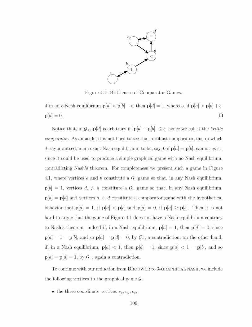
b
<
d
f
a
e
=
1
Figure 4.1: Brittleness of Comparator Games.
if in an ǫ-Nash equilibrium p[a] < p[b] − ǫ, then p[d] = 1, whereas, if p[a] > p[b] + ǫ,
p[d] = 0.
Notice that, in G<, p[d] is arbitrary if |p[a]−p[b]| ≤ ǫ; hence we call it the brittle
comparator. As an aside, it is not hard to see that a robust comparator, one in which
d is guaranteed, in an exact Nash equilibrium, to be, say, 0 if p[a] = p[b], cannot exist,
since it could be used to produce a simple graphical game with no Nash equilibrium,
contradicting Nash’s theorem. For completeness we present such a game in Figure
4.1, where vertices e and b constitute a G1 game so that, in any Nash equilibrium,
p[b] = 1, vertices d, f , a constitute a G= game so that, in any Nash equilibrium,
p[a] = p[d] and vertices a, b, d constitute a comparator game with the hypothetical
behavior that p[d] = 1, if p[a] < p[b] and p[d] = 0, if p[a] ≥ p[b]. Then it is not
hard to argue that the game of Figure 4.1 does not have a Nash equilibrium contrary
to Nash’s theorem: indeed if, in a Nash equilibrium, p[a] = 1, then p[d] = 0, since
p[a] = 1 = p[b], and so p[a] = p[d] = 0, by G=, a contradiction; on the other hand,
if, in a Nash equilibrium, p[a] < 1, then p[d] = 1, since p[a] < 1 = p[b], and so
p[a] = p[d] = 1, by G=, again a contradiction.
To continue with our reduction from Brouwer to 3-graphical nash, we include
the following vertices to the graphical game G.
• the three coordinate vertices vx, vy, vz,
106
• for i ∈ 1, 2, . . . , n, vertices vbi(x), vbi(y) and vbi(z), whose p-values correspond
to the i-th most significant bit of p[vx], p[vy], p[vz],
• for i ∈ 1, 2, . . . , n, vertices vxi, vyi
and vzi, whose p-values correspond to
the fractional number resulting from subtracting from p[vx], p[vy], p[vz] the
fractional numbers corresponding to the i − 1 most significant bits of p[vx],
p[vy], p[vz] respectively.
We can extract these values by computing the binary representation of ⌊p[vx]2n⌋
and, similarly, for vy and vz, that is, the binary representations of the integers i, j, k
such that (x, y, z) = (p[vx],p[vy],p[vz]) lies in the cubelet Kijk. This is done by a
graphical game that simulates, using the arithmetical gadgets of Lemmas 4.2 and 4.3,
the following algorithm (< (a, b) is 1 if a ≤ b and 0 if a > b):
x1 = x;
for i = 1, . . . , n do:
bi(x) :=< (2−i, xi); xi+1 := xi − bi(x) · 2−i;
similarly, for y and z;
This is accomplished in G by connecting these vertices as prescribed by Lemmas 4.2
and 4.3, so that p[vxi],p[vbi(x)], etc. approximate the value of xi, bi(x) etc. as computed
by the above algorithm. The following lemma (when applied with m = n) shows that
this device properly decodes the first n bits of the binary expansion of x = p[vx], as
long as x is not too close to a multiple of 2−n (suppose ǫ << 2−n to be fixed later).
Lemma 4.4. For m ≤ n, if∑m
i=1 bi2−i + 3mǫ < p[vx] <
∑mi=1 bi2
−i + 2−m − 3mǫ
for some b1, . . . , bm ∈ 0, 1, then, in every ǫ-Nash equilibrium of G, p[vbj(x)] = bj,
and p[vxj+1] = p[vx] −∑j
i=1 bi2−i ± 3jǫ, for all j ≤ m.
Proof. The proof is by induction on j. For j = 1, the hypothesis∑m
i=1 bi2−i + 3mǫ <
107
p[vx] <∑m
i=1 bi2−i + 2−m − 3mǫ implies, in particular, that
b1
2+ 3ǫ ≤
m∑
i=1
bi2−i + 3mǫ < p[vx] <
m∑
i=1
bi2−i + 2−m − 3mǫ ≤ b1
2+
1
2− 3ǫ
and, since p[vx1 ] = p[vx] ± ǫ, it follows that
b1
2+ 2ǫ < p[vx1 ] <
b1
2+
1
2− 2ǫ.
By Lemma 4.3, this implies that p[vb1(x)] = b1; note that the preparation of the
constant 12
—against which a comparator game compares the value p[vx1 ]— is done
via a G 12
game which introduces an error of ±ǫ. For the computation of p[vx2 ],
the multiplication of p[vb1(x)] by 12
and the subtraction of the product from p[vx1 ]
introduce an error of ±ǫ each and, therefore, p[vx2 ] = p[vx1 ] − b112± 2ǫ. And, since
p[vx1 ] = p[vx] ± ǫ, it follows that p[vx2 ] = p[vx] − b112± 3ǫ, as required.
Supposing that the claim holds up to j−1 ≤ m−1, we will show that it holds for
j. By the induction hypothesis, we have that p[vxj] = p[vx]−∑j−1
i=1 bi2−i ± 3(j − 1)ǫ.
Combining this with∑m
i=1 bi2−i + 3mǫ < p[vx] <
∑mi=1 bi2
−i + 2−m − 3mǫ, it follows
that
m∑
i=j
bi2−i + 3(m − (j − 1))ǫ < p[vxj
] <m∑
i=j
bi2−i + 2−m − 3(m − (j − 1))ǫ
which implies
bj
2j+ 2ǫ < p[vxj
] <bj
2j+
1
2j− 2ǫ.
Continue as in the base case.
Assuming that x = p[vx], y = p[vy], z = p[vz] are all at distance greater than
3nǫ from any multiple of 2−n, the part of G that implements the above algorithm
computes i, j, k such that the point (x, y, z) lies in the cubelet Kijk; that is, there
108
are 3n vertices of the game G whose p values are equal to the n bits of the binary
representation of i, j, k. Once we have the binary representations of i, j, k, we can
feed them into another part of G that simulates the circuit C. We could simulate
the circuit by having vertices that represent gates, using addition (with ceiling 1)
to simulate or, multiplication for and, and 1 − x for negation. However, there is
a simpler way, one that avoids the complications related to accuracy, to simulate
Boolean functions under the assumption that the inputs are 0 or 1:
Lemma 4.5. There are binary graphical games G∨,G∧,G¬ with two input players a, b
(one input player a for G¬) and an output player c such that the payoffs of a and b
do not depend on the choices of c, and, at any ǫ-Nash equilibrium with ǫ < 1/4 in
which p[a],p[b] ∈ 0, 1, p[c] is also in 0, 1, and is in fact the result of applying the
corresponding Boolean function to the inputs.
Proof. These games are in the same spirit as G<. In G∨, for example, the payoff to
c is 1/2 if it plays 0; if c plays 1 its payoff is 1 if at least one of a, b plays 1, and it is
0 if they both play 0. Similarly, for G∧ and G¬.
It would seem that all we have to do now is to close the loop as follows: in addition
to the part of G that computes the bits of i, j, k, we could have a part that simulates
circuit C in the neighborhood of Kijk and decides whether among the vertices of the
cubelet Kijk there is a panchromatic one; if not, the vertices vx, vy and vz could be
incentivized to change their p values, say in the direction δC(i,j,k), otherwise stay put.
To simulate a circuit evaluation in G we could have one vertex for each gate of the
circuit so that, in any ǫ-Nash equilibrium in which all the p[vbi(x)]’s are 0 − 1, the
vertices corresponding to the outputs of the circuit also play pure strategies, and,
furthermore, these strategies correspond correctly to the outputs of the circuit.
But, as we mentioned above, there is a problem: Because of the brittle compara-
tors, at the boundaries of the cubelets the vertices that should represent the values
109

of the bits of i, j, k hold in fact arbitrary reals and, therefore, so do the vertices
that represent the outputs of the circuit, and this noise in the calculation can create
spurious Nash equilibria. Suppose for example that (x, y, z) lies on the boundary
between two cubelets that have color 1, i.e. their centers are assigned vector δ1 by C,
and none of these cubelets have a panchromatic vertex. Then there ought not to be
a Nash equilibrium with p[vx] = x, p[vy] = y, p[vz] = z. We would want that, when
p[vx] = x, p[vy] = y, p[vz ] = z, the vertices vx, vy, vz have the incentive to shift their
p values in direction δ1, so that vx prefers to increase p[vx]. However, on a boundary
between two cubelets, some of the “bit values” that get loaded into the vertices vbi(x),
could be other than 0 and 1, and then there is nothing we can say about the output
of the circuit that processes these values.
To overcome this difficulty, we resort to the following averaging maneuver: We
repeat the above computation not just for the point (x, y, z), but also for all M =
(2m+1)3 points of the form (x+p·α, y+q ·α, z+s·α), for −m ≤ p, q, s ≤ m, where m
is a large enough constant to be fixed later (we show below that m = 20 is sufficient).
The vertices vx, vy, vz are then incentivized to update their values according to the
consensus of the results of these computations, most of which are reliable, as we shall
show next.
Let us first describe this averaging in more detail. It will be convenient to assume
that the output of C is a little more explicit than 3 bits: let us say that C computes
six bits ∆x+, ∆x−, ∆y+, ∆y−, ∆z+, ∆z−, such that at most one of ∆x+, ∆x− is 1,
at most one of ∆y+, ∆y− is 1, and, similarly, for z, and the increment of the Brouwer
function at the center of Kijk is α · (∆x+ − ∆x−, ∆y+ − ∆y−, ∆z+ − ∆z−), equal to
one of the vectors δ0, δ1, δ2, δ3 specified in the definition of Brouwer, where recall
α = 2−2n.
The game G has the following structure: Starting from (x, y, z), some part of the
110
game is devoted to calculating the points (x+p·α, y+q·α, z+s·α), −m ≤ p, q, s ≤ m.
Then, another part evaluates the circuit C on the binary representation of each of
these points yielding 6M output bits, ∆x+1 , . . . , ∆z−M . A final part calculates the
following averages
(δx+, δy+, δz+) =α
M
M∑
t=1
(∆x+t , ∆y+
t , ∆z+t ), (4.1)
(δx−, δy−, δz−) =α
M
M∑
t=1
(∆x−t , ∆y−
t , ∆z−t ), (4.2)
which correspond to the average positive, respectively negative, shift of all M points.
We have already described above how to implement the bit extraction and the
evaluation of a circuit using the gadgets of Lemmas 4.2, 4.3 and 4.5. The computation
of points (x + p · α, y + q · α, z + s · α), for all −m ≤ p, q, s ≤ m, is also easy to
implement by preparing the values α|p|, α|q|, α|s|, using gadgets Gα|p|, Gα|q|, Gα|s|,
and then adding or subtracting the results to x, y and z respectively, depending on
whether p is positive or not and, similarly, for q and s. Of course, these computations
are subject to truncations at 0 and 1 (see Lemma 4.2).
To implement the averaging of Equations (4.1) and (4.2) we must be careful on
the order of operations. Specifically, we first have to multiply the 6 outputs, ∆x+t ,
∆x−t , ∆y+
t , ∆y−t , ∆z+
t , ∆z−t , of each circuit evaluation by αM
using the G× αM
gadget
and, having done so, we then implement the additions (4.1) and (4.2). Since α will
be a very small constant, by doing so we avoid undesired truncations at 0 and 1.
We can now close the loop by inserting equality, addition and subtraction gadgets,
G=, G+, G−, that force, at equilibrium, x to be equal to (x′ + δx+)−δx−, where x′ is a
copy of x created using G=, and, similarly, for y and z. Note that in G we respect the
order of operations when implementing (x′+δx+)−δx− to avoid undesired truncations
at 0 or 1 as we shall see next. This concludes the reduction; it is clear that it can be
111
carried out in polynomial time.
Our proof is concluded by the following claim. For the following lemma we choose
ǫ = α2. Recall from our definition of Brouwer that α = 2−2n.
Lemma 4.6. In any ǫ-Nash equilibrium of the game G, one of the vertices of the
cubelet(s) that contain (p[vx],p[vy],p[vz]) is panchromatic.
Proof. We start by pointing out a simple property of the increments δ0, . . . , δ3:
Lemma 4.7. Suppose that for nonnegative integers k0, . . . , k3 all three coordinates of
∑3i=0 kiδi are smaller in absolute value than αK
5where K =
∑3i=0 ki. Then all four
ki are positive.
Proof. For the sake of contradiction, suppose that k1 = 0. It follows that k0 < K/5
(otherwise the negative x coordinate of∑3
i=0 kiδi would be too large), and thus one
of k2, k3 is larger than 2K/5, which makes the corresponding coordinate of∑3
i=0 kiδi
too large, a contradiction. Similarly, if k2 = 0 or k3 = 0. Finally, if k0 = 0 then one
of k1, k2, k3 is at least K/3 and the associated coordinate of∑3
i=0 kiδi at least αK/3,
again a contradiction.
Let us denote by vδx+ , v∆x+t1≤t≤M the vertices of G that represent the values δx+,
∆x+t 1≤t≤M . To implement the averaging
δx+ =α
M
M∑
t=1
∆x+t
inside G, we first multiply each p[v∆x+t
] by αM
using a G αM
gadget, and then sum the
results by a sequence of addition gadgets. Since each of these operations induces an
error of ±ǫ and there are 2M − 1 operations it follows that
p[vδx+ ] =α
M
M∑
t=1
p[v∆x+t
] ± (2M − 1)ǫ. (4.3)
112
Similarly, denoting by vδx− , v∆x−t1≤t≤M the vertices of G that represent the values
δx−, ∆x−t 1≤t≤M , it follows that
p[vδx− ] =α
M
M∑
t=1
p[v∆x−t
] ± (2M − 1)ǫ, (4.4)
and, similarly, for directions y and z.
We continue the proof by distinguishing two subcases for the location of (x, y, z) =
(p[vx],p[vy],p[vz])
(a) the point (p[vx],p[vy],p[vz]) is further than (m + 1)α from every face of the
cube [0, 1]3,
(b) the point (p[vx],p[vy],p[vz]) is at distance at most (m + 1)α from some face of
the cube [0, 1]3.
Case (a): Denoting by vx+p·α the player of G that represents x+p ·α, the small value
of ǫ relative to α implies that at most one of the values p[vx+p·α], −m ≤ p ≤ m, can
be 3nǫ-close to a multiple of 2−n, and, similarly, for the directions y and z. Indeed,
recall that x + p · α is computed from x by first preparing the value |p|α via a G|p|α
gadget and then adding or subtracting the result to x —depending on whether p is
positive or not— using G+ or G−. It follows that
p[vx+p·α] = p[vx] + p · α ± 2ǫ, (4.5)
since each gadget introduces an error of ±ǫ, where note that there are no truncations
at 0 or 1, because, by assumption, (m + 1)α < p[vx] < 1 − (m + 1)α. Consequently,
for p > p′,
p[vx+p·α] − p[vx+p′·α] ≥ (p − p′) · α − 4ǫ > 6nǫ,
113
and, moreover,
p[vx+m·α] − p[vx−m·α] ≤ 2m · α + 4ǫ << 2−n, (4.6)
since m is a constant, α = 2−2n, ǫ = α2, and n is assumed to be large enough. Hence,
from among the M = (2m + 1)3 circuit evaluations, all but at most 3(2m + 1)2, or at
least K = (2m − 2)(2m + 1)2, compute legitimate, i.e. binary, ∆x+ etc. values.
Let us denote by K ⊆ −m, . . . , m3, |K| ≥ K, the set of values (p, q, r) for which
the bit extraction from (p[vx+p·α],p[vy+q·α],p[vz+r·α]) results in binary outputs and,
consequently, so does the circuit evaluation. Let
SK =α
M
∑
t∈K(p[v∆x+
t] − p[v∆x−
t],p[v∆y+
t] − p[v∆y−
t],p[v∆z+
t] − p[v∆z−t
]), (4.7)
SKc =α
M
∑
t/∈K(p[v∆x+
t] − p[v∆x−
t],p[v∆y+
t] − p[v∆y−
t],p[v∆z+
t] − p[v∆z−t
]). (4.8)
Recall that we have inserted gadgets G+, G− and G= in G to enforce that in a Nash
equilibrium x = x′ + δx+ − δx−, where x′ is a copy of x. Because of the defection of
the gadgets this will not be exactly tight in an ǫ-Nash equilibrium. More precisely,
denoting by vx′ the player of G corresponding to x′, the following are true in an ǫ-Nash
equilibrium
p[vx′ ] = p[vx] ± ǫ
p[vx] = p[v′x] + p[vδx+ ] − p[vδx− ] ± 2ǫ,
where for the second observe that both p[vδx+ ] and p[vδx− ] are bounded above by
α + (2M − 1)ǫ so there will be no truncations at 0 or 1 when adding p[vδx+ ] to p[v′x]
114

and then subtracting p[vδx− ]. By combining the above we get
p[vδx+ ] − p[vδx− ] = ±3ǫ
and, similarly, for y and z
p[vδy+ ] − p[vδy− ] = ±3ǫ
p[vδz+ ] − p[vδz− ] = ±3ǫ.
Now, if we use (4.3), (4.4), (4.7), (4.8) we derive
∣∣SKℓ+ SKc
ℓ
∣∣ ≤ (4M + 1)ǫ, for ℓ = x, y, z,
where SKℓ, SKc
ℓis the ℓ coordinate of SK, SKc . Moreover, since |K| ≥ K, the sum-
mation SKcℓ
has at most M − K summands and because each of them is at most αM
in absolute value it follows that |SKcℓ| ≤ α
M(M − K), for all ℓ = x, y, z. Therefore,
we have that
∣∣SKℓ
∣∣ ≤ (4M + 1)ǫ +M − K
Mα, for ℓ = x, y, z.
Finally, note by the definition of the set K that, for all (p, q, r) ∈ K, the bit extraction
from (p[vx+p·α],p[vy+q·α],p[vz+r·α]) and the following circuit evaluation result in bi-
nary outputs. Therefore, SK = 1M
∑3i=0 kiδi for some nonnegative integers k0, . . . , k3
adding up to |K|. From the above we get that
∣∣∣3∑
i=0
kiδi
∣∣∣∞
≤ (4M + 1)Mǫ + (M − K)α ≤ (4M + 1)Mǫ + 3(2m + 1)2α.
By choosing m = 20, the bound becomes less than αK/5, and so Lemma 4.7 applies.
It follows that, among the results of the |K| circuit computations, all four δ0, . . . , δ3
115
appeared. And, since every point on which the circuit C is evaluated is within ℓ1 dis-
tance at most 3mα + 6ǫ << 2−n from the point (x, y, z), as Equation (4.5) dictates,
this implies that among the corners of the cubelet(s) containing (x, y, z) there must
be one panchromatic corner, completing the proof of Lemma 4.6 for case (a).
Case (b): We will show that there is no ǫ-Nash equilibrium in which (p[vx],p[vy],p[vz])
is within distance (m + 1)α from a face of [0, 1]3. We will argue so only for the case
p[vx] ≤ (m + 1)α,
(m + 1)α < p[vy] < 1 − (m + 1)α,
(m + 1)α < p[vz ] < 1 − (m + 1)α;
the other cases follow similarly.
First, we show that, for all −m ≤ p ≤ m, the bit extraction from p[vx+p·α] results
in binary outputs. From the proof of Lemma 4.4 it follows that, to show this, it is
enough to establish that p[vx+pα] < 2−n − 3nǫ, for all p. Indeed, for p ≥ 0, Equation
(4.5) applies because there are no truncations at 1 at the addition gadget. So for
p ≥ 0 we get
p[vx+p·α] ≤ p[vx] + p · α + 2ǫ ≤ (m + 1)α + mα + 2ǫ << 2−n − 3nǫ
On the other hand, for p < 0, there might be a truncation at 0 when we subtract the
value |p|α from p[vx]. Nevertheless, we have that
p[vx+p·α] = max 0 , p[vx] − (|p|α ± ǫ) ± ǫ ≤ p[vx] + 2ǫ
≤ (m + 1)α + 2ǫ << 2−n − 3nǫ.
116
Therefore, for all −m ≤ p ≤ m, the bit extraction from p[vx+p·α] is successful, i.e.
results in binary outputs.
For the directions y and z the picture is exactly the same as in case (a) and,
therefore, there exists at most one q,−m ≤ q ≤ m, and at most one r, −m ≤ r ≤ m,
for which the bit extraction from p[vy+q·α] and p[vz+r·α] fails. Therefore, from among
the M = (2m+1)3 points of the form (p[vx+p·α],p[vy+q·α],p[vz+r·α]) the bit extraction
succeeds in all but at most 2(2m + 1)2 of them.
Therefore, at least K ′ = (2m − 1)(2m + 1)2 circuit evaluations are successful,
i.e. in binary arithmetic, and, moreover, they correspond to points inside cubelets
of the form Kijk with i = 0. In particular, from Equation (4.6) and the analogous
equations for the y and z coordinates, it follows that the successful circuit evaluations
correspond to points inside at most 4 neighboring cubelets of the form K0jk. Since
these cubelets are adjacent to the x = 0 face of the cube, from the properties of
the circuit C in the definition of the problem Brouwer, it follows that, among the
outputs of these evaluations, one of the vectors δ0, δ1, δ2, δ3 is missing. Without loss
of generality, let us assume that δ0 is missing. Then, since there are K ′ successful
evaluations, one of δ1, δ2, δ3 appears at least K ′/3 times.
If this is vector δ1 (a similar argument applies for the cases δ2, δ3), then denoting
by vx′+δx+ the player corresponding to x′ + δx+, the following should be true in an
ǫ-Nash equilibrium.
p[vx] + ǫ ≥ p[vx′ ] ≥ p[vx] − ǫ,
α + (2M − 1)ǫ ≥ p[vδx+ ] ≥ K ′
3Mα − (2M − 1)ǫ,
p[vx′+δx+ ] ≥ min(1,p[vx′] + p[vδx+ ]) − ǫ ≥ p[vx′ ] + p[vδx+ ] − ǫ,
M − K ′
Mα + (2M − 1)ǫ ≥ p[vδx− ],
p[vx] ≥ max(0,p[vx′+δx+ ] − p[vδx− ]) − ǫ ≥ p[vx′+δx+ ] − p[vδx− ] − ǫ;
117
in the second inequality of the third line above, we used that p[vx] ≤ (m + 1)α.
Combining the above we get
p[vx] ≥ p[vx′] + p[vδx+ ] − p[vδx− ] − 2ǫ
≥ p[vx] + p[vδx+ ] − p[vδx− ] − 3ǫ
or equivalently that
p[vδx− ] ≥ p[vδx+ ] − 3ǫ,
which implies
M − K ′
Mα + (4M + 1)ǫ ≥ K ′
3Mα,
which is not satisfied by our selection of parameters.
To conclude the proof of Theorem 4.1, if we find any ǫ-Nash equilibrium of G,
Lemma 4.6 has shown that by reading off the first n binary digits of p[vx], p[vy] and
p[vz] we obtain a solution to the corresponding instance of Brouwer.
4.2 Two-Player Games
Soon after our proof became available, Chen and Deng [CD06] showed that our PPAD-
completeness result can be extended to the important two-player case. Here we
present a rather simple modification of our proof from the previous section establishing
this result.
Theorem 4.8 ([CD06]). 2-Nash is PPAD-complete.
Proof. Let us define d-additive graphical Nash to be the problem d-graphical
Nash restricted to bipartite graphical games with additive utility functions defined
next.
118
Definition 4.9. Let GG be a graphical game with underlying graph G = (V, E). We
call GG a bipartite graphical game with additive utility functions if G is a bipartite
graph and, moreover, for each vertex v ∈ V and for every pure strategy sv ∈ Sv of that
player, the expected payoff of v for playing the pure strategy sv is a linear function
of the mixed strategies of the vertices in Nv \ v with rational coefficients; that is,
there exist rational numbers αsvu,su
u∈Nv\v,su∈Su, αsvu,su
∈ [0, 1] for all u ∈ N (v)\v,
su ∈ Su, such that the expected payoff to vertex v for playing pure strategy sv is
∑
u∈Nv\v,su∈Su
αsvu,su
p[u : su],
where p[u : su] denotes the probability that vertex u plays pure strategy su.
The proof is based on the following lemmas.
Lemma 4.10. Brouwer is poly-time reducible to 3-additive graphical Nash.
Lemma 4.11. 3-additive graphical Nash is poly-time reducible to 2-Nash.
Proof of Lemma 4.10: The reduction is almost identical to the one in the proof
of Theorem 4.1. Recall that given an instance of Brouwer a graphical game was
constructed using the gadgets Gα,G×α,G=,G+,G−,G∗, G∨,G∧,G¬, and G>. In fact,
gadget G∗ is not required, since only multiplication by a constant is needed which can
be accomplished via the use of gadget G×α. Moreover, it is not hard to see by looking
at the payoff tables of the gadgets defined in Section 3.1 and Lemma 4.3 that, in
gadgets Gα, G×α, G=, G+, G−, and G>, the non-input vertices have the additive utility
functions property of Definition 4.9. Let us further modify the games G∨,G∧,G¬ so
that their output vertices have the additive utility functions property.
Lemma 4.12. There are binary graphical games G∨,G∧,G¬ with two input players
a, b (one input player a for G¬) and an output player c such that the payoffs of a and
b do not depend on the choices of c, c’s payoff satisfies the additive utility functions
119

property, and, in any ǫ-Nash equilibrium with ǫ < 1/4 in which p[a],p[b] ∈ 0, 1,
p[c] is also in 0, 1, and is in fact the result of applying the corresponding Boolean
function to the inputs.
Proof. For G∨, the payoff of player c is 0.5p[a]+0.5p[b] for playing 1 and 14
for playing
0. For G∧, the payoff of player c is 0.5p[a] + 0.5p[b] for playing 1 and 34
for playing 0.
For G¬, the payoff of player c is p[a] for playing 0 and p[a : 0] for playing 1.
If the modified gadgets G∨,G∧,G¬ specified by Lemma 4.12 are used in the con-
struction of Theorem 4.1, all vertices of the resulting graphical game satisfy the
additive utility functions property of Definition 4.9. To make sure that the graphical
game is also bipartite we modify the gadgets G∨,G∧,G¬, and G> with the insertion of
an extra output vertex. The modification is the same for all 4 gadgets: let c be the
output vertex of any of these gadgets; we introduce a new output vertex e, whose pay-
off only depends on the strategy of c, but c’s payoff does not depend on the strategy
of e, and such that the payoff of e is p[c] for playing 1 and p[c : 0] for playing 0 (i.e.
e “copies” c, if c’s strategy is pure). It is not hard to see that, for every gadget, the
new output vertex has the same behavior with regards to the strategies of the input
vertices as the old output vertex, as specified by Lemmas 4.3 and 4.12. Moreover,
it is not hard to verify that the graphical game resulting from the construction of
Theorem 4.1 with the use of the modified gadgets G∨,G∧,G¬, and G> is bipartite;
indeed, it is sufficient to color blue the input and output vertices of all G×α, G=, G+,
G−, G∨, G∧, G¬, and G> gadgets used in the construction, blue the output vertices of
all Gα gadgets used, and red the remaining vertices. 2
Proof of Lemma 4.11: Let GG be a bipartite graphical game of maximum degree 3
with additive utility functions and GG the graphical game resulting after rescaling all
utilities to the set [0, 1], e.g. by dividing all utilities by max u, where max u is the
largest entry in the payoff tables of game GG. Also, let ǫ < 1. In time polynomial in
120
|GG|+log(1/ǫ), we will specify a 2-player normal-form game G and an accuracy ǫ′ with
the property that, given an ǫ′-Nash equilibrium of G, one can recover in polynomial
time an ǫ-Nash equilibrium of GG. This will be enough, since an ǫ-Nash equilibrium
of GG is trivially an ǫ · max u-Nash equilibrium of game GG and, moreover, |GG| is
polynomial in |GG|.
The construction of G from GG is almost identical to the one described in Fig-
ure 3.5. Let V = V1⊔V2 be the bipartition of the vertices of set V so that all edges are
between a vertex in V1 and a vertex in V2. Let us define c : V → 1, 2 as c(v) = 1 iff
v ∈ V1 and let us assume, without loss of generality, that |v : c(v) = 1| = |v : c(v) = 2|;
otherwise, we can add to GG isolated vertices to make up any shortfall. Suppose that
n is the number of vertices in GG (after the possible addition of isolated vertices) and
t the cardinality of the strategy sets of the vertices in V , and let ǫ′ = ǫ/n. Let us then
employ the Steps 4 and 5 of the algorithm in Figure 3.5 to construct the normal-form
game G from the graphical game GG; however, we choose M = 6tnǫ
, and modify Step
5b to read as follows
(b)’ for v ∈ V and sv ∈ Sv, if c(v) = p and s contains (v, sv) and (u, su) for some
u ∈ N (v) \ v, su ∈ Su, then ups = αsv
u,su,
where we used the notation from Definition 4.9.
We argue next that, given an ǫ′-Nash equilibrium xp(v,a)p,v,a of G, xv
av,a is an
ǫ-Nash equilibrium of GG, where
xva = x
c(v)(v,a)
/∑
j∈Sv
xc(v)(v,j), ∀v ∈ V, a ∈ Sv.
Suppose that p = c(v) for some vertex v of the graphical game GG. As in the proof
of Theorem 3.8, Lemma 3.11, it can be shown that in any ǫ′-Nash equilibrium of the
121

game G,
Pr[p plays v] ∈[
2
n− 1
M,
2
n+
1
M
].
Now, without loss of generality assume that p = 1 (the pursuer) and suppose v is
vertex v(p)i , in the notation of Figure 3.5. Then, in an ǫ′-Nash equilibrium of the game
G, we have, by the definition of a Nash equilibrium, that for all strategies sv, s′v ∈ Sv
of vertex v:
E [payoff to p for playing (v, sv)] > E [payoff to p for playing (v, s′v)] + ǫ′ ⇒ xp(v,s′v) = 0.
(4.9)
But
E [payoff to p for playing (v, sv)] = M ·Pr[p + 1 plays v
(p+1)i
]+
∑
u∈Nv\v,su∈Su
αsvu,su
xc(u)(u,su)
and, similarly, for s′v. Therefore, (4.9) implies
∑
u∈Nv\v,su∈Su
αsvu,su
xc(u)(u,su) >
∑
u∈Nv\v,su∈Su
αs′vu,su
xc(u)(u,su) + ǫ′ ⇒ xp
(v,s′v) = 0. (4.10)
Lemma 4.13. For all v, a ∈ Sv,
∣∣∣∣∣xva −
xc(v)(v,a)
2/n
∣∣∣∣∣ ≤n
2M.
Proof. We have
∣∣∣∣∣xva −
xc(v)(v,a)
2/n
∣∣∣∣∣ =
∣∣∣∣∣x
c(v)(v,a)
Pr[c(v) plays v]−
xc(v)(v,a)
2/n
∣∣∣∣∣
=x
c(v)(v,a)
Pr[c(v) plays v]
|Pr[c(v) plays v] − 2/n|2/n
≤ n
2M,
122
where we used that∑
j∈Svx
c(v)(v,j) = Pr[c(v) plays v] and |Pr[c(v) plays v] − 2/n| ≤
1M
.
By (4.10) and Lemma 4.13, we get that, for all v ∈ V , sv, s′v ∈ Sv,
∑
u∈Nv\v,su∈Su
αsvu,su
xusu
>∑
u∈Nv\v,su∈Su
αs′vu,su
xusu
+n
2ǫ′ + |Nv \ v|t
n
M⇒ xv
s′v= 0.
Since n2ǫ′ + |Nv \ v|t n
M≤ ǫ, it follows that xv
av,a is an ǫ-Nash equilibrium of the
game GG. 2
4.3 Other Classes of Games and Fixed Points
There are several special cases of the Nash equilibrium problem for which PPAD-
hardness persists. It has been shown, for example, that finding a Nash equilibrium of
two-player normal-form games in which all utilities are restricted to take values 0 or 1
(the so-called win-lose case) remains PPAD-complete [AKV05, CTV07]. The Nash
equilibrium problem in two-player symmetric games — that is, games in which the
two players have the same strategy sets, and their utility is the same function of their
own and the other player’s strategy — is also PPAD-complete. 1 Moreover, rather
surprisingly, it is essentially PPAD-complete to even play repeated games [BCI+08]
(the so-called “Folk Theorem for repeated games” [Rub79] notwithstanding).
And, what is known about the complexity of the Nash Equilibrium problem in
other classes of succinctly representable games with many players (besides the graphi-
cal games which we have resolved)? For example, are these problems even in PPAD? 2
In [DFP06], we provide a general sufficient condition, satisfied by all known succinct
1This follows from a symmetrization argument of von Neumann [BN50] providing a reductionfrom the Nash equilibrium problem in general two-player games to that in symmetric games (see,also, the construction of Gale, Kuhn, Tucker [GKT50]).
2It is typically easy to see that they cannot be easier than the normal-form case.
123
representations of games, such as congestion games [Ros73, FPT04] and extensive-
form games [OR94], for membership of the Nash equilibrium problem in the class
PPAD. The basic idea is using the “arithmetical” gadgets in our present proof to
simulate the calculation of utilities in these succinct games.
Our techniques can be used to treat two other open problems in complexity. One
is that of the complexity of simple stochastic games defined in [Con92], heretofore
known to be in TFNP, but not in any of the more specialized classes like PPAD or
PLS. Now, it is known that this problem is equivalent to evaluating combinational
circuits with max, min, and average gates. Since all three kinds of gates can be
implemented by the graphical games in our construction, it follows that solving simple
stochastic games is in PPAD. 3
Similarly, by an explicit construction we can show the following.
Theorem 4.14. Let p : [0, 1] → R be any polynomial function such that p(0) < 0 and
p(1) > 0. Then there exists a graphical game in which all vertices have two strategies,
0 and 1, and in which the mixed Nash equilibria correspond to a particular vertex v
playing strategy 1 with probability equal to the roots of p(x) between 0 and 1.
Proof Sketch. Let p be described by its coefficients α0, α1, . . . , αn, so that
p(x) := αnxn + αn−1x
n−1 + . . . + α1x + α0.
Taking A := (∑n
i=0 |αi|)−1, it is easy to see that the range of the polynomial q(x) :=
12Ap(x) + 1
2is [0, 1], that q(0) < 1
2, q(1) > 1/2, and that every point r ∈ [0, 1] such
that q(r) = 12
is a root of p. We define next a graphical game GG in which all vertices
have two strategies, 0 and 1, and a designated vertex v of GG satisfies the following
(i) in any mixed Nash equilibrium of GG the probability xv1 by which v plays strat-
egy 1 satisfies q(xv1) = 1/2;
3One has to pay attention to the approximation; see [EY07] for details.
124
(ii) for any root r of p in [0, 1], there exists a mixed Nash equilibrium of GG in
which xv1 = r;
The graphical game has the following structure:
• there is a component graphical game GGq with an “input vertex” v and an
“output vertex” u such that, in any Nash equilibrium of GG, the mixed strategies
of u and v satisfy xu1 = q(xv
1); a graphical game which progressively performs the
computations required for the evaluation of q(·) on xv1 can be easily constructed
using our game-gadgets; note that the computations can be arranged in such
an order that no truncations at 0 or 1 happen (recall the rescaling by 12A and
the shifting around 1/2 done above);
• a comparator game G> (see Lemma 4.3) compares the mixed strategy of u with
the value 12, prepared by a G1/2 gadget (see Section 3.1), so that the output
vertex of the comparator game plays 0 if xu1 > 1
2, 1 if xu
1 < 12, and anything if
xu1 = 1
2;
• we identify the output player of G> with player v;
It is not hard to see that GG satisfies Properties (i) and (ii).
As a corollary of Theorem 4.14, it follows that fixed points of polynomials can be
computed by computing (exact) Nash equilibria of graphical games. Computing fixed
points of polynomials via exact Nash equilibria in graphical games can be extended
to the multi-variate case again via the use of game gadgets to evaluate the polynomial
and the use of a series of G= gadgets to set the output equal to the input.
Both this result and the result about simple stochastic games noted above were
shown independently by [EY07], while Theorem 4.14 was already shown by Bubelis
[Bub79].
125

Chapter 5
Computing Approximate
Equilibria
In the previous chapters, we establish that r-Nash is PPAD-complete, for r ≥ 2.
This result implies that it is PPAD-complete to compute an ǫ-Nash equilibrium of a
normal-form game with at least two players, for any approximation ǫ scaling as an
inverse exponential function of the size of game. The same is true for graphical games
of degree 3 or larger, since d-graphical Nash was also shown to be PPAD-complete,
for all d ≥ 3. This brings about the following question.
• Is computing an ǫ-Nash equilibrium easier, if ǫ is larger?
It turns out that, for any ǫ which is inverse polynomial in n, computing an ǫ-
Nash equilibrium of a 2-player n-strategy game remains PPAD-complete. This result,
established by Chen, Deng and Teng [CDT06a], follows from a modification of our
reduction in which the starting Brouwer problem is defined not on the 3-dimensional
cube, but on the n-dimensional hypercube. Intuitively, the difference is this: In order
to create the exponentially many cells needed to embed the “line” of the end of the
line problem, our construction had to resort to exponentially small cell size. On the
other hand, the n-dimensional hypercube contains exponentially many cells, all of
126
reasonably large size. This observation implies that approximation which is inverse
polynomial in n is sufficient to encode the end of the line instance into a 2-player
n-strategy game. In fact, the same negative result can be extended to graphical
games: For any ǫ which is inverse polynomial in n, computing an ǫ-Nash equilibrium
of a n-player graphical game of degree 3 is PPAD-complete. So, for both normal-form
and graphical games, a fully polynomial-time approximation scheme seems unlikely.
The following important question emerges at the boundary of intractability.
• Is there a polynomial-time approximation scheme for the Nash equilibrium problem?
We discuss this question in its full generality in Section 5.1. We also present special
classes of two-player games for which there exists a polynomial-time approximation
scheme, and we conclude the section with a discussion of challenges towards ob-
taining a polynomial-time approximation scheme for general two-player games. In
Sections 5.2 through 5.9, we consider a broad and important class of games, called
anonymous games, for which we present a polynomial-time approximation scheme.
5.1 General Games and Special Classes
The problem of computing approximate equilibria was considered by Lipton, Markakis
and Mehta in [LMM03], where a quasi-polynomial-time algorithm was given for nor-
malized normal-form games. 1 This algorithm is based upon the realization that,
in every r-player game, there exists an ǫ-approximate Nash equilibrium in which all
players’ mixed strategies have support of size O(
r2 log(r2n)ǫ2
). Hence, an ǫ-approximate
equilibrium can be found by exhaustive search over all mixed strategy profiles with
this support size. Despite extensive research on the subject, no improvement of this
result is known for general values of ǫ. For fixed values of ǫ, we have seen a se-
1Most of the research on computing approximate Nash equilibria has focused on normalizedgames; since the approximation is defined in the additive sense this decision is a reasonable one.
127
quence of results, computing ǫ-Nash equilibria of normalized 2-player games with
ǫ = .5 [DMP06], .39 [DMP07], .37 [BBM07]; the best known ǫ at the time of writing
is .34 [TS07].
Our knowledge for multiplayer games is also quite limited. In [DP08a], we show
that an ǫ-Nash equilibrium of a normalized normal-form game with two strategies
per player can be computed in time nO(log log n+log 1ǫ), where n is the size of the game.
For graphical games of constant degree, where our hardness result from Chapter 4
comes in the picture, a similar algorithm is unlikely, since it would imply that PPAD
has quasi-polynomial-time algorithms. 2 On the positive side, Elkind, Goldberg and
Goldberg show that a Nash equilibrium of graphical games with maximum degree 2
and 2 strategies per player can be computed in polynomial time [EGG06]. And what is
known about larger degrees? In [DP06], we describe a polynomial-time approximation
scheme for normalized graphical games with a constant number of strategies per
player, bounded degree, and treewidth which is at most logarithmic in the number
of players. Whether this result can be extended to graphical games with super-
logarithmic treewidth remains an important open problem.
Since our knowledge for general games is limited, it is natural to ask the following.
• Are there special classes of games for which approximate equilibria can be computed
efficiently?
Recall that two-player zero-sum games are solvable exactly in polynomial time
by Linear Programming [Neu28, Dan63, Kha79]. Kannan and Theobald extend this
tractability result by providing a polynomial-time approximation scheme for a gen-
eralization of two-player zero-sum games, called low-rank games [KT07]. These are
games in which the sum of the players’ payoff matrices3 is a matrix of fixed rank.
2Recall that, as noted before, finding an ǫ-Nash equilibrium of bounded degree graphical gamesremains PPAD-complete for values of ǫ scaling inverse polynomially with the number of players.
3In two-player games, the payoffs of the players can be described by specifying two n×n matricesR and C, where n is the number of strategies of the players, so that Rij and Cij is respectively the
128
In [DP08b], we observe that a PTAS exists for another class of two-player games,
called bounded-norm games, in which every player’s payoff matrix is the sum of a
constant matrix and a matrix with bounded infinity norm. These games have been
shown to be PPAD-complete [CDT06b]. Hence, our tractability result exhibits a
rare class of games which are PPAD-complete to solve exactly, yet a polynomial-time
approximation scheme exists for solving them approximately.
In view of these positive results for special classes of two-player games, the fol-
lowing question arises.
• Is there a polynomial-time approximation scheme for general two-player games?
It is well-known that, if a two-player game has a Nash equilibrium in which both
players’ strategies have support of some fixed size, then that equilibrium can be re-
covered in polynomial time. Indeed, all we need to do is to perform an exhaustive
search over all possible supports for the two players. For the right choice of sup-
ports, the Nash equilibrium can be found by solving a linear program. However, this
straightforward approach does not extend beyond fixed size supports, since in this
case the number of possible supports becomes super-polynomial.
• Is it then the case that supports of size linear in the number of strategies are hard?
Surprisingly, we show that this not always the case [DP08b]: If a two-player
game has a Nash equilibrium in which both players’ strategies spread non-trivially
(that is, with significant probability mass) over a linear-size subset of the strategies,
then an ǫ-Nash equilibrium can be recovered in randomized polynomial time, for
any ǫ. Observe that the PPAD-hard instances of two-player games constructed in
Section 4.2 only have equilibria of (non-trivial) linear support. Hence, our positive
result for linear supports is another case of a problem which is PPAD-complete to
payoff of the first and the second player, if the first player chooses her i-th strategy and the secondplayer chooses her j-th strategy.
129
solve exactly, yet a randomized polynomial-time approximation scheme exists for
solving it approximately. It also brings about the following question.
• If neither fixed nor linear, what support sizes are hard?
The following discussion seems to suggest that logarithmic size supports are hard.
It turns out that our PTAS for both the case of linear size support and the class of
bounded-norm games, discussed previously, is of a very special kind, called oblivious.
This means that it looks at a fixed set of pairs of mixed strategies, by sampling a
distribution over that set, and uses the input game only to determine whether the
sampled pair of mixed strategies constitutes an approximate Nash equilibrium. The
guarantee in our algorithms is that an approximate Nash equilibrium is sampled with
inverse polynomial probability, so that only a polynomial number of samples is needed
in expectation.
We show, however, that an oblivious PTAS does not exist for general two-player
games [DP08b]. And here is how logarithmic support comes into play. In our proof,
we define a family of 2-player n-strategy games, indexed by all subsets of strategies
of about logarithmic size, with the following property: The game indexed by a subset
S satisfies that, in any ǫ-Nash equilibrium, the mixed strategy of one of the players is
within total variation distance O(ǫ) from the uniform distribution over S. Since there
are nΘ(log n) subsets of size log n, it is not hard to deduce that any oblivious algorithm
should have expected running time nΩǫ(log n), that is super-polynomial. Incidentally,
note that the (also oblivious) algorithm of Lipton, Markakis and Mehta [LMM03]
runs in time nΘ(log n/ǫ2), and it works by exhaustively searching over all multisets of
strategies of size Θ(log n/ǫ2).
It is natural to conjecture that an important step towards obtaining a polynomial-
time approximation scheme for two-player games is to understand how an approxi-
mate Nash equilibrium can be computed in the presence of an exact Nash equilibrium
130
of logarithmic support.
5.2 Anonymous Games
In the rest of this chapter, we consider algorithms for computing approximate equilib-
ria in a very broad and important class of games, called anonymous games. These are
games in which the players’ payoff functions, although potentially different, do not
differentiate among the identities of the other players. That is, each player’s payoff
depends on the strategy that she chooses and only the number of the other players
choosing each of the available strategies. An immediate example is traffic: The delay
incurred by a driver depends on the number of cars on her route, but not on the identi-
ties of the drivers. Another example arises in certain auction settings where the utility
of a bidder is affected by the distribution of the other bids, but not on the identities
of the other bidders. In fact, many problems of interest for algorithmic game theory,
such as congestion games, participation games, voting games, and certain markets
and auctions, are anonymous. The reader is referred to [Mil96, Blo99, Blo05, Kal05]
for recent work on the subject by economists.
Note that anonymous games are much more general than symmetric games, in
which all players are identical. In fact, any normal-form game can be represented
by an anonymous game as follows. Two-player games are obviously anonymous for
trivial reasons. To encode a multi-player non-anonymous game into an anonymous
game, we can give to each player the option of choosing a strategy belonging to any
player of the original game, but, at the same time, punish a player who chooses
a strategy belonging to another player. Observe that this encoding incurs only a
polynomial blowup in description complexity if the starting game has a constant
number of players. Hence, all hardness results from the previous chapters apply to
this case.
131
We are going to focus instead on anonymous games with many players and a
few strategies per player. Observe that, if n is the number of players and k the
number of strategies, only O(nk) numbers are needed to specify the game. Hence,
anonymous games are a rare case of multiplayer games that have a polynomially
succinct representation — as long as the number k of strategies is fixed. Our main
result is a polynomial-time approximation scheme for such games.
Our PTAS extends to several generalizations of anonymous games, for example the
case in which there are a few types of players, and the utilities depend on how many
players of each type play each strategy; and to the case in which we have extended
families (disjoint graphical games of constant degree and with logarithmically many
players, each with a utility depending in arbitrary (possibly non-anonymous) ways
on their neighbors in the graph, in addition to their anonymous —possibly typed—
interest on everybody else). This generalizations are discussed in Section 5.8. Observe
that, if we allowed larger extended families, we would be able to embed in the game
graphical games with super-logarithmic size, for which the intractability result of the
previous chapters comes into play.
Let us conclude our introduction to anonymous games with a discussion resonating
the introduction to this dissertation in Chapter 1. Algorithmic Game Theory aspires
to understand the Internet and the markets it encompasses and creates, hence the
study of multiplayer games is of central importance. We believe that our PTAS is
a positive algorithmic result spanning a vast expanse in this space. Because of the
tremendous analytical difficulties detailed in Sections 5.5 through 5.7, our algorithm
is not practical (as we shall see, the number of strategies and the accuracy appear
in the exponent of the running time). It could be, of course, the precursor of more
practical algorithms; in fact, we discuss a rather efficient algorithm for the case of
two strategies in Section 5.9. But, more importantly, our algorithm should be seen
as compelling computational evidence that there are very extensive and important
132
classes of common games which are free of the negative implications of our complexity
result from the previous chapters.
The structure of the remaining of this chapter is the following: In Section 5.3, we
define anonymous games formally and introduce some useful notation. In Section 5.4,
we state our main result and discuss our proof techniques. In Section 5.5, we state
our main technical lemma and show how it implies the PTAS, and, in Section 5.6, we
discuss its proof, which we give in Section 5.7. In Section 5.8, we discuss extensions of
our PTAS to broader classes of games, and, in Section 5.9, we discuss more efficient
PTAS’s.
5.3 Definitions and Notation
A (normalized) anonymous game is a triple G = (n, k, upi ) where [n] = 1, . . . , n,
n ≥ 2, is a set of players, [k] = 1, . . . , k, k ≥ 2, is a set of strategies, and upi
with p ∈ [n] and i ∈ [k] is the utility of player p when she plays strategy i, a
function mapping the set of partitions Πkn−1 = (x1, . . . , xk) : xi ∈ N0 for all i ∈
[k],∑k
i=1 xi = n−1 to the interval [0, 1]. 4 This means that the payoff of each player
depends on her own strategy and only the number of the other players choosing each
of the k strategies. Let us denote by ∆kn−1 the convex hull of the set Πk
n−1. That is,
∆kn−1 = (x1, . . . , xk) : xi ≥ 0 for all i ∈ [k],
∑ki=1 xi = n − 1.
A mixed strategy profile is a set of n distributions δp ∈ ∆kp∈[n], where by ∆k
we denote the (k − 1)-dimensional simplex, or, equivalently, the set of distributions
over [k]. In this notation, a mixed strategy profile is an ǫ-Nash equilibrium if, for all
p ∈ [n] and j, j′ ∈ [k],
Eδ1,...,δnupj (x) > Eδ1,...,δnup
j′(x) + ǫ ⇒ δp(j′) = 0,
4As we noted in Section 5.1, the literature on Nash approximation studies normalized games sothat the approximation error is additive.
133
where x is drawn from Πkn−1 by drawing n−1 random samples from [k] independently
according to the distributions δq, q 6= p, and forming the induced partition. Notice
the similarity to (2.2) in Chapter 2.
Similarly, a mixed strategy profile is an ǫ-approximate Nash equilibrium if, for
all p ∈ [n] and j ∈ [k], Eδ1,...,δnupi (x) + ǫ ≥ Eδ1,...,δnup
j(x), where i is drawn from
[k] according to δp and x is drawn from Πkn−1 as above, by drawing n − 1 random
samples from [k] independently according to the distributions δq, q 6= p, and forming
the induced partition.
Our working assumptions are that n is large and k is fixed; notice that, in this
case, anonymous games are succinctly representable [PR05], in the sense that their
representation requires specifying O(nk) numbers, as opposed to the nkn numbers
required for general games. Arguably, succinct games are the only multiplayer games
that are computationally meaningful; see [PR05] for an extensive discussion of this
point.
5.4 A Polynomial-Time Approximation Scheme for
Anonymous Games
Our main result is a PTAS for anonymous games with a few strategies, namely
Theorem 5.1. There is a PTAS for the mixed Nash equilibrium problem for normal-
ized anonymous games with a constant number of strategies.
We provide the proof of the theorem in the next section, where we also describe the
basic technical lemma needed for the proof. Let us give here instead some intuition
about our proof techniques. The basic idea of our algorithm is extremely simple
and intuitive: Instead of performing the search for an approximate Nash equilibrium
over the full set of mixed strategy profiles, we restrict our attention to mixed strate-
134
gies assigning to each strategy in their support probability mass which is an integer
multiple of 1z, where z is a large enough natural number. We call this process dis-
cretization. Searching the space of discretized mixed strategy profiles can be done
efficiently with dynamic programming. Indeed, there are less than (z + 1)k−1 dis-
cretized mixed strategies available to each player, so at most n(z+1)k−1−1 partitions
of the number n of players into these discretized mixed strategies. And checking if
there is an approximate Nash equilibrium consistent with such a partition can be
done efficiently using a max-flow argument (see details in the proof of Theorem 5.1
given in Section 5.5).
The challenge, however, lies somewhere else: We need to establish that any mixed
Nash equilibrium of the original game is close to a discretized mixed strategy profile.
And this requires the following non-trivial approximation lemma for multinomial dis-
tributions: The distribution of the sum of n independent random unit vectors with
values ranging over e1, . . . , ek, where ei is the unit vector along dimension i of the
k-dimensional Euclidean space, can be approximated by the distribution of the sum
of another set of independent unit vectors whose probabilities of obtaining each value
are multiples of 1z, and so that the variational distance of the two distributions de-
pends only on z (in fact, a decreasing function of z) and the dimension k, but not
on the number of vectors n. In our setting, the original random vectors correspond
to the strategies of the players in a Nash equilibrium, and the discretized ones to the
discretized mixed strategy profile. The total variation distance bounds the approxi-
mation error incurred by replacing the Nash equilibrium with the discretized mixed
strategy profile.
The approximation lemma needed in our proof can be interpreted as constructing
a surprisingly sparse cover of the set of multinomial-sum distributions under the
total variation distance. Covers have been considered extensively in the literature of
approximation algorithms, but we know of no non-trivial result working in the set of
135

multinomial-sum distributions or producing a cover of the required sparsity to achieve
a polynomial-time approximation scheme for the Nash equilibrium in anonymous
games. In the next section, we state the precise approximation result that we need
and show how it can be used to derive a PTAS for anonymous games with a constant
number of strategies. In Section 5.6, we discuss the challenges in establishing this
result, and the full proof is given in Section 5.7.
5.5 An Approximation Theorem for Multinomial
Distributions
Before stating our result, let us define the total variation distance between two dis-
tributions P and Q over a finite set A as
||P − Q||TV =1
2
∑
α∈A|P(α) − Q(α)|.
Similarly, if X and Y are two random variables ranging over a finite set, their total
variation distance, denoted
||X − Y ||TV ,
is defined to be the total variation distance between their distributions. Our approx-
imation result is the following.
Theorem 5.2. Let pi ∈ ∆ki∈[n], and let Xi ∈ Rki∈[n] be a set of independent k-
dimensional random unit vectors such that, for all i ∈ [n], ℓ ∈ [k], Pr[Xi = eℓ] = pi,ℓ,
where eℓ is the unit vector along dimension ℓ; also, let z > 0 be an integer. Then
there exists another set of probability vectors pi ∈ ∆ki∈[n] such that
1. |pi,ℓ − pi,ℓ| = O(
1z
), for all i ∈ [n], ℓ ∈ [k];
2. pi,ℓ is an integer multiple of 12k
1z, for all i ∈ [n], ℓ ∈ [k];
136
3. if pi,ℓ = 0, then pi,ℓ = 0, for all i ∈ [n], ℓ ∈ [k];
4. if Xi ∈ Rki∈[n] is a set of independent random unit vectors such that Pr[Xi =
eℓ] = pi,ℓ, for all i ∈ [n], ℓ ∈ [k], then
∣∣∣∣∣
∣∣∣∣∣∑
i
Xi −∑
i
Xi
∣∣∣∣∣
∣∣∣∣∣TV
= O
(f(k)
log z
z1/5
)(5.1)
and, moreover, for all j ∈ [n],
∣∣∣∣∣
∣∣∣∣∣∑
i6=j
Xi −∑
i6=j
Xi
∣∣∣∣∣
∣∣∣∣∣TV
= O
(f(k)
log z
z1/5
), (5.2)
where f(k) is an exponential function of k estimated in the proof.
In other words, there is a way to quantize any set of n independent random vectors
into another set of n independent random vectors, whose probabilities of obtaining
each value are integer multiples of ǫ ∈ [0, 1], so that the total variation distance be-
tween the distribution of the sum of the vectors before and after the quantization is
bounded by O(f(k)2k/6ǫ1/6). The important, and perhaps surprising, property of this
bound is the lack of dependence on the number n of random vectors. From this, the
proof of Theorem 5.1 follows.
Proof of Theorem 5.1: Consider a mixed Nash equilibrium (p1, . . . , pn) of the
game. We claim that the mixed strategy profile (p1, . . . , pn) specified by Theorem 5.2
constitutes a O(f(k)z−16 )-Nash equilibrium. Indeed, for every player i ∈ [n] and
every pure strategy m ∈ [k] for that player, let us track down the change in the
expected utility of the player for playing strategy m when the distribution over Πkn−1
defined by the pjj 6=i is replaced by the distribution defined by the pjj 6=i. It is
not hard to see that the absolute change is bounded by the total variation distance
between the distributions of the random vectors∑
j 6=i Xj and∑
j 6=i Xj , where Xjj 6=i
137
are independent random vectors distributed according to the distributions pjj 6=i
and, similarly, Xjj 6=i are independent random vectors distributed according to the
distributions pjj 6=i.5 Hence, by Theorem 5.2, the change in the utility of the player
is at most O(f(k)z−16 ), which implies that the pi’s constitute an O(f(k)z−
16 )-Nash
equilibrium of the game. If we take z =(
f(k)ǫ
)6
, this is a δ-Nash equilibrium, for
δ = O(ǫ).
From the previous discussion it follows that there exists a mixed strategy profile
pii which is of the very special kind described by Property 2 in the statement of
Theorem 5.2 and constitutes a δ-Nash equilibrium of the given game, if we choose
z =(
f(k)ǫ
)6
. The problem is, of course, that we do not know such a mixed strategy
profile and, moreover, we cannot afford to do exhaustive search over all mixed strategy
profiles satisfying Property 2, since there is an exponential number of those. We do
instead the following search which is guaranteed to find a δ-Nash equilibrium.
Notice first that there are at most (2kz)k = 2k2(
f(k)ǫ
)6k
=: K “quantized” mixed
strategies with each probability being a multiple of 12k
1z, z =
(f(k)
ǫ
)6
. Let K be
the set of such quantized mixed strategies. We start our algorithm by guessing the
partition of the number n of players into quantized mixed strategies; let θ = θσσ∈K
be the partition, where θσ represents the number of players choosing the discretized
mixed strategy σ ∈ K. Now we only need to determine if there exists an assignment
of mixed strategies to the players in [n], with θσ of them playing mixed strategy
σ ∈ K, so that the corresponding mixed strategy profile is a δ-Nash equilibrium. To
answer this question it is enough to solve the following max-flow problem. Let us
consider the bipartite graph ([n],K, E) with edge set E defined as follows: (i, σ) ∈ E,
for i ∈ [n] and σ ∈ K, if θσ > 0 and σ is a δ-best response for player i, if the
partition of the other players into the mixed strategies in K is the partition θ, with
5The proof of this bound is similar to the derivation of the bound (3.14) in the proof ofLemma 3.32, using also that the game is anonymous and normalized, i.e., all utilities lie in [0, 1].
138
one unit subtracted from θσ. 6 Note that to define E expected payoff computations are
required. By straightforward dynamic programming, the expected utility of player
i for playing pure strategy s ∈ [k] given the mixed strategies of the other players
can be computed with O(knk) operations on numbers with at most b(n, z, k) :=
⌈1 + n(k + log2 z) + log2(1/umin)⌉ bits, where umin is the smallest non-zero payoff
value of the game. 7 To conclude the construction of the max-flow instance we add a
source node u connected to all the left hand side nodes and a sink node v connected
to all the right hand side nodes. We set the capacity of the edge (σ, v) equal to θσ, for
all σ ∈ K, and the capacity of all other edges equal to 1. If the max-flow from u to v
has value n then there is a way to assign discretized mixed strategies to the players so
that θσ of them play mixed strategy σ ∈ K and the resulting mixed strategy profile is
a δ-Nash equilibrium (details omitted). There are at most (n+1)K−1 possible guesses
for θ; hence, the search takes overall time
O((nKk2nkb(n, z, k) + p(n + K + 2)) · (n + 1)K−1
),
where p(n + K + 2) is the time needed to find an integral maximum flow in a graph
with n + K + 2 nodes and edge-weights encoded with at most ⌈log2 n⌉ bits. Hence,
the overall time is
nO
„
2k2( f(k)
ǫ )6k
«
· log2(1/umin).
2
6For our discussion, a mixed strategy σ of player i is a δ-best response to a set of mixed strategiesfor the other players iff the expected payoff of player i for playing any pure strategy s in the supportof σ is no more than δ worse than her expected payoff for playing any pure strategy s′.
7To compute a bound on the number of bits required for the expected utility computations, notethat the expected utility is positive, cannot exceed 1, and its smallest possible non-zero value is atleast ( 1
2k
1
z)numin, since the mixed strategies of all players are from the set K.
139
5.6 Discussion of Proof Techniques
Observe first that, from a technical perspective, the k = 2 case of Theorem 5.2 is
inherently different than the k > 2 case. Indeed, when k = 2, knowledge of the number
of players who selected their first strategy determines the whole partition of the
number of players into strategies; therefore, in this case the probabilistic experiment
is in some sense one-dimensional. On the other hand, when k > 2, knowledge of the
number of “balls in a bin”, that is, the number of players who selected a particular
strategy, does not provide full information about the number of balls in the other bins.
This complication would be quite benign if the vectors Xi were identically distributed,
since in this case the number of balls in a bin would at least characterize precisely
the probability distribution of the number of balls in the other bins (as a multinomial
distribution with one bin less and the bin-probabilities appropriately renormalized).
But, in our case, the vectors Xi are not identically distributed. Hence, already for
k = 3 the problem is fundamentally different than the k = 2 case.
Indeed, it turns out that obtaining the result for the k = 2 case is easier. Here
is the intuition: If the expectation of every Xi at the first bin was small, their sum
would be distributed like a Poisson distribution (marginally at that bin); if the expec-
tation of every Xi was large, the sum would be distributed like a (discretized) Normal
distribution. 8 So, to establish the result we can do the following (see [DP07] for
details): First, we cluster the Xi’s into those with small and those with large expec-
tation at the first bin, and then we discretize the Xi’s separately in the two clusters
in such a way that the sum of their expectations (within each cluster) is preserved to
within the discretization accuracy. To show the closeness in total variation distance
between the sum of the Xi’s before and after the discretization, we compare instead
8Comparing, in terms of variational distance, a sum of independent Bernoulli random variablesto a Poisson or a Normal distribution is an important problem in probability theory. The approxi-mations we use are obtained by applications of Stein’s method [BC05, BHJ92, R07].
140
the Poisson or Normal distributions (depending on the cluster) which approximate
the sum of the Xi’s: For the “small cluster”, we compare the Poisson distributions
approximating the sum of the Xi’s before and after the discretization. For the “large
cluster”, we compare the Normals approximating the sum of the Xi’s before and after
the discretization.
One would imagine that a similar technique, i.e., approximating by a multidimen-
sional Poisson or Normal distribution, would work for the k > 2 case. Comparing a
sum of multinomial random variables to a multidimensional Poisson or Normal distri-
bution is a little harder in many dimensions (see the discussion in [Bar05]), but almost
optimal bounds are known for both the multidimensional Poisson [Bar05, Roo98] and
the multidimensional Normal [Bha75, G91] approximations. Nevertheless, these re-
sults by themselves are not sufficient for our setting: Approximating by a multidi-
mensional Normal performs very poorly at the coordinates where the vectors have
small expectations, and approximating by a multidimensional Poisson fails at the
coordinates where the vectors have large expectations. And in our case, it could
very well be that the sum of the Xi’s is distributed like a multidimensional Poisson
distribution in a subset of the coordinates and like a multidimensional Normal in the
complement (those coordinates where the Xi’s have respectively small or large expec-
tations). What we really need, instead, is a multidimensional approximation result
that combines the multidimensional Poisson and Normal approximations in the same
picture; and such a result is not known.
Our approach instead is very indirect. We define an alternative way of sampling
the vectors Xi which consists of performing a random walk on a binary decision tree
and performing a probabilistic choice between two strategies at the leaves of the tree
(Sections 5.7.1 and 5.7.2). The random vectors are then clustered so that, within
a cluster, all vectors share the same decision tree (Section 5.7.3), and the rounding,
performed separately for every cluster, consists of discretizing the probabilities for the
141
probabilistic experiments at the leaves of the tree (Section 5.7.4). The rounding is
done in such a way that, if all vectors Xi were to end up at the same leaf after walking
on the decision tree, then the one-dimensional result described above would apply for
the (binary) probabilistic choice that the vectors are facing at the leaf. However, the
random walks will not all end up at the same leaf with high probability. To remedy
this, we define a coupling between the random walks of the original and the discretized
vectors for which, in the typical case, the probabilistic experiments that the original
vectors are running at every leaf of the tree are very “similar” to the experiments that
the discretized vectors are running. That is, our coupling guarantees that, with high
probability over the random walks, the total variation distance between the choices
(as random variables) that are to be made by the original vectors at every leaf of
the decision tree and the choices (again as random variables) that are to be made by
the discretized vectors is very small. The coupling of the random walks is defined in
Section 5.7.5, and a quantification of the similarity of the leaf experiments under this
coupling is given in Section 5.7.6.
For a discussion about why naive approaches such as rounding to the closest dis-
crete distribution or randomized rounding do not appear useful, even for the k = 2
case, see Section 3.1 of [DP07].
5.7 Proof of the Multinomial Approximation The-
orem
5.7.1 The Trickle-Down Process
Consider the mixed strategy pi of player i. The crux of our argument is an alternative
way to sample from this distribution, based on the so-called trickle-down process,
defined next.
142
TDP — Trickle-Down Process
Input: (S, p), where S = i1, . . . , im ⊆ [k] is a set of strategies and p a probability
distribution p(ij) > 0 : j = 1, . . . , m. We assume that the elements of S are ordered
i1, . . . , im in such a way that (a) p(i2) is the largest of the p(ij)’s and (b) for 2 6= j <
j′ 6= 2, p(ij) ≤ p(ij′). That is, the largest probability is second, and, other than that,
the probabilities are sorted in non-decreasing order (ties broken lexicographically).
if |S| ≤ 2 stop; else apply the partition and double operation:
1. let ℓ∗ < m be the (unique) index such that∑
ℓ<ℓ∗ p(iℓ) ≤ 12
and∑
ℓ>ℓ∗ p(iℓ) < 12;
2. Define the two sets SL = iℓ : ℓ ≤ ℓ∗ and SR = iℓ : ℓ ≥ ℓ∗
3. Define the probability distribution pL such that, for all ℓ < ℓ∗, pL(iℓ) = 2p(iℓ).
Also, let t := 1 −∑ℓ∗−1ℓ=1 pL(iℓ); if t = 0, then remove ℓ∗ from SL, otherwise
set pL(iℓ∗) = t. Similarly, define the probability distribution pR such that
pR(iℓ) = 2p(iℓ), for all ℓ > ℓ∗ and pR(iℓ∗) = 1 −∑mℓ∗+1 pR(iℓ). Notice that,
because of the way we have ordered the strategies in S, iℓ∗ is neither the first
nor the last element of S in our ordering, and hence 2 ≤ |SL|, |SR| < |S|.
4. call TDP(SL, pL); call TDP(SR, pR);
That is, TDP splits the support of the mixed strategy of a player into a tree of
finer and finer sets of strategies, with all leaves having just two strategies. At each
level the two sets in which the set of strategies is split overlap in at most one strategy
(whose probability mass is divided between its two copies). The two sets then have
probabilities adding up to 1/2, but then the probabilities are multiplied by 2, so that
each node of the tree represents a distribution.
143
5.7.2 An Alternative Sampling of the Random Vectors
Let pi be the mixed strategy of player i, and Si be its support. 9 The execution
of TDP(Si, pi) defines a rooted binary tree Ti with node set Vi and set of leaves
∂Ti. Each node v ∈ Vi is identified with a pair (Sv, pi,v), where Sv ⊆ [k] is a set of
strategies and pi,v is a distribution over Sv. Based on this tree, we define the following
alternative way to sample Xi:
Sampling Xi
1. (Stage 1) Perform a random walk from the root of the tree Ti to the leaves,
where, at every non-leaf node, the left or right child is chosen with probability
1/2; let Φi ∈ ∂Ti be the (random) leaf chosen by the random walk;
2. (Stage 2) Let (S, p) be the label assigned to the leaf Φi, where S = ℓ1, ℓ2; set
Xi = eℓ1 , with probability p(ℓ1), and Xi = eℓ2 , with probability p(ℓ2).
The following lemma, whose straightforward proof we omit, states that this is
indeed an alternative sampling of the mixed strategy of player i.
Lemma 5.3. For all i ∈ [n], the process Sampling Xi outputs Xi = eℓ with proba-
bility pi,ℓ, for all ℓ ∈ [k].
5.7.3 Clustering the Random Vectors
We use the process TDP to cluster the random vectors of the set Xii∈[n], by defining
a cell for every possible tree structure. More formally, for some α > 0 to be determined
later in the proof,
Definition 5.4 (Cell Definition). Two vectors Xi and Xj belong to the same cell if
9In this section and the following two sections we assume that |Si| > 1; if not, we set pi = pi,and all claims we make in Sections 5.7.5 and 5.7.6 are trivially satisfied.
144
• there exists a tree isomorphism fi,j : Vi → Vj between the trees Ti and Tj such
that, for all u ∈ Vi, v ∈ Vj, if fi,j(u) = v, then Su = Sv, and in fact the elements
of Su and Sv are ordered the same way by pi,u and pj,v.
• if u ∈ ∂Ti, v = fi,j(u) ∈ ∂Tj , and ℓ∗ ∈ Su = Sv is the strategy with the smallest
probability mass for both pi,u and pj,v, then either pi,u(ℓ∗), pj,v(ℓ∗) ≤ ⌊zα⌋
zor
pi,u(ℓ∗), pj,v(ℓ∗) > ⌊zα⌋
z; the leaf is called Type A leaf in the first case, Type B
leaf in the second case.
It is easy to see that the total number of cells is bounded by a function of k only,
call it g(k). The following claim provides an estimate of g(k).
Claim 5.5. Any tree resulting from TDP has at most k − 1 leaves, and the total
number of cells is bounded by g(k) = kk22k−12kk!.
5.7.4 Discretization within a Cell of the Clustering
Recall that our goal is to “discretize” the probabilities in the distribution of the Xi’s.
We will do this separately in every cell of our clustering. In particular, supposing
that Xii∈I is the set of vectors falling in a particular cell, for some index set I, we
will define a set of “discretized” vectors Xii∈I in such a way that, for h(k) = k2k,
and for all j ∈ I,
∣∣∣∣∣
∣∣∣∣∣∑
i∈IXi −
∑
i∈IXi
∣∣∣∣∣
∣∣∣∣∣TV
= O(h(k) log z · z−1/5); (5.3)
∣∣∣∣∣∣
∣∣∣∣∣∣
∑
i∈I\jXi −
∑
i∈I\jXi
∣∣∣∣∣∣
∣∣∣∣∣∣TV
= O(h(k) log z · z−1/5). (5.4)
We establish these bounds in Section 5.7.5. Using the bound on the number of cells
in Claim 5.5, an easy application of the coupling lemma implies the bounds shown
in (5.1) and (5.2) for f(k) := h(k) · g(k), thus concluding the proof of Theorem 5.2.
145
We shall henceforth concentrate on a particular cell containing the vectors Xii∈I ,
for some I ⊆ [n]. Since the trees Tii∈I are isomorphic, for notational convenience
we shall denote all those trees by T . To define the vectors Xii∈I we must provide,
for all i ∈ I, a distribution pi : [k] → [0, 1] such that Pr[Xi = eℓ] = pi(ℓ), for all
ℓ ∈ [k]. To do this, we assign to all Xii∈I the tree T and then, for every leaf
v ∈ ∂T and i ∈ I, define a distribution pi,v over the two-element ordered set Sv,
by the Rounding process below. Then the distribution pi is implicitly defined as
pi(ℓ) =∑
v∈∂T :ℓ∈Sv2−depthT (v)pi,v(ℓ).
Rounding: for all v ∈ ∂T with Sv = ℓ1, ℓ2, ℓ1, ℓ2 ∈ [k] do the following
1. find a set of probabilities pi,ℓ1i∈I with the following properties
• for all i ∈ I, |pi,ℓ1 − pi,v(ℓ1)| ≤ 1z;
• for all i ∈ I, pi,ℓ1 is an integer multiple of 1z;
•∣∣∑
i∈I pi,ℓ1 −∑
i∈I pi,v(ℓ1)∣∣ ≤ 1
z;
2. for all i ∈ I, set pi,v(ℓ1) := pi,ℓ1, pi,v(ℓ2) := 1 − pi,ℓ1;
Finding the set of probabilities required by Step 1 of the Rounding process is
straightforward and the details are omitted (see [DP07], Section 3.3 for a way to
do so). It is now easy to check that the set of probability vectors pii∈I satisfies
Properties 1, 2 and 3 of Theorem 5.2.
5.7.5 Coupling within a Cell of the Clustering
We are now coming to the main part of the proof: Showing that the variational
distance between the original and the discretized distribution within a cell depends
only on z and k. We will only argue that our discretization satisfies (5.3); the proof
of (5.4) is identical.
Before proceeding let us introduce some notation. Specifically,
146
• let Φi ∈ ∂T be the leaf chosen by Stage 1 of the process Sampling Xi and
Φi ∈ ∂T the leaf chosen by Stage 1 of Sampling Xi;
• let Φ = (Φi)i∈I and let G denote the distribution of Φ; similarly, let Φ = (Φi)i∈I
and let G denote the distribution of Φ.
Moreover, for all v ∈ ∂T , with Sv = ℓ1, ℓ2 and ordering (ℓ1, ℓ2),
• let Iv ⊆ I be the (random) index set such that i ∈ Iv iff i ∈ I ∧ Φi = v and,
similarly, let Iv ⊆ I be the (random) index set such that i ∈ Iv iff i ∈ I∧Φi = v;
• let Jv,1,Jv,2 ⊆ Iv be the (random) index sets such i ∈ Jv,1 iff i ∈ Iv ∧ Xi = eℓ1
and i ∈ Jv,2 iff i ∈ Iv ∧ Xi = eℓ2 ;
• let Tv,1 = |Jv,1|, Tv,2 = |Jv,2| and let Fv denote the distribution of Tv,1;
• let T := ((Tv,1, Tv,2))v∈∂T and let F denote the distribution of T ;
• let Jv,1, Jv,2, Tv,1, Tv,2, T , Fv, F be defined similarly.
The following is easy to see, so we postpone its proof to the appendix.
Claim 5.6. For all θ ∈ (∂T )I , G(θ) = G(θ).
Since G and G are the same distribution we will henceforth denote that distri-
bution by G. The following lemma is sufficient to conclude the proof of Theorem
5.2.
Lemma 5.7. There exists a value of α, used in the definition of the cells, such that,
for all v ∈ ∂T ,
G
(θ : ||Fv(·|Φ = θ) − Fv(·|Φ = θ)||TV ≤ O
(2k log z
z1/5
))≥ 1 − 4
z1/3,
where Fv(·|Φ) denotes the conditional probability distribution of Tv,1 given Φ and,
similarly, Fv(·|Φ) denotes the conditional probability distribution of Tv,1 given Φ.
147
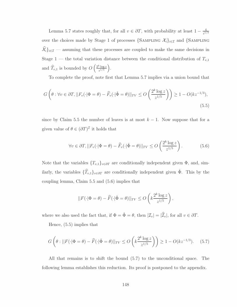
Lemma 5.7 states roughly that, for all v ∈ ∂T , with probability at least 1 − 4z1/3
over the choices made by Stage 1 of processes Sampling Xii∈I and Sampling
Xii∈I — assuming that these processes are coupled to make the same decisions in
Stage 1 — the total variation distance between the conditional distribution of Tv,1
and Tv,1 is bounded by O(
2k log zz1/5
).
To complete the proof, note first that Lemma 5.7 implies via a union bound that
G
(θ : ∀v ∈ ∂T, ||Fv(·|Φ = θ) − Fv(·|Φ = θ)||TV ≤ O
(2k log z
z1/5
))≥ 1 − O(kz−1/3),
(5.5)
since by Claim 5.5 the number of leaves is at most k − 1. Now suppose that for a
given value of θ ∈ (∂T )I it holds that
∀v ∈ ∂T, ||Fv(·|Φ = θ) − Fv(·|Φ = θ)||TV ≤ O
(2k log z
z1/5
). (5.6)
Note that the variables Tv,1v∈∂T are conditionally independent given Φ, and, sim-
ilarly, the variables Tv,1v∈∂T are conditionally independent given Φ. This by the
coupling lemma, Claim 5.5 and (5.6) implies that
||F (·|Φ = θ) − F (·|Φ = θ)||TV ≤ O
(k
2k log z
z1/5
),
where we also used the fact that, if Φ = Φ = θ, then |Iv| = |Iv|, for all v ∈ ∂T .
Hence, (5.5) implies that
G
(θ : ||F (·|Φ = θ) − F (·|Φ = θ)||TV ≤ O
(k
2k log z
z1/5
))≥ 1 − O(kz−1/3). (5.7)
All that remains is to shift the bound (5.7) to the unconditional space. The
following lemma establishes this reduction. Its proof is postponed to the appendix.
148
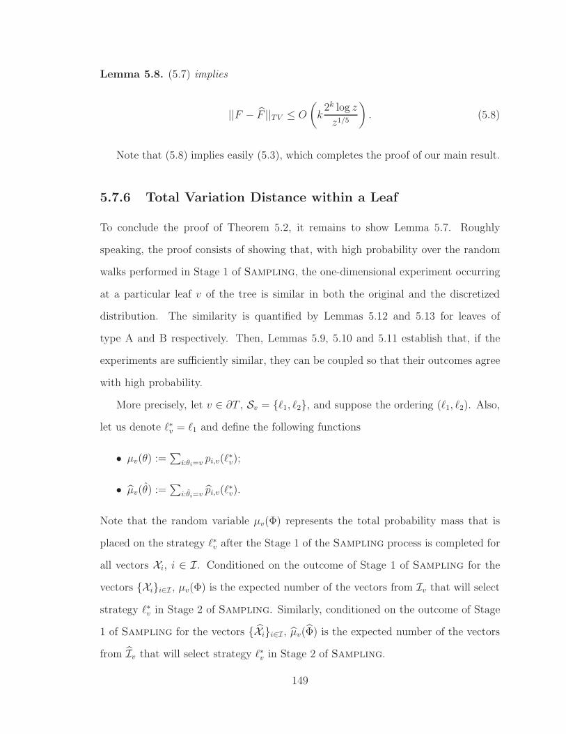
Lemma 5.8. (5.7) implies
||F − F ||TV ≤ O
(k
2k log z
z1/5
). (5.8)
Note that (5.8) implies easily (5.3), which completes the proof of our main result.
5.7.6 Total Variation Distance within a Leaf
To conclude the proof of Theorem 5.2, it remains to show Lemma 5.7. Roughly
speaking, the proof consists of showing that, with high probability over the random
walks performed in Stage 1 of Sampling, the one-dimensional experiment occurring
at a particular leaf v of the tree is similar in both the original and the discretized
distribution. The similarity is quantified by Lemmas 5.12 and 5.13 for leaves of
type A and B respectively. Then, Lemmas 5.9, 5.10 and 5.11 establish that, if the
experiments are sufficiently similar, they can be coupled so that their outcomes agree
with high probability.
More precisely, let v ∈ ∂T , Sv = ℓ1, ℓ2, and suppose the ordering (ℓ1, ℓ2). Also,
let us denote ℓ∗v = ℓ1 and define the following functions
• µv(θ) :=∑
i:θi=v pi,v(ℓ∗v);
• µv(θ) :=∑
i:θi=v pi,v(ℓ∗v).
Note that the random variable µv(Φ) represents the total probability mass that is
placed on the strategy ℓ∗v after the Stage 1 of the Sampling process is completed for
all vectors Xi, i ∈ I. Conditioned on the outcome of Stage 1 of Sampling for the
vectors Xii∈I , µv(Φ) is the expected number of the vectors from Iv that will select
strategy ℓ∗v in Stage 2 of Sampling. Similarly, conditioned on the outcome of Stage
1 of Sampling for the vectors Xii∈I , µv(Φ) is the expected number of the vectors
from Iv that will select strategy ℓ∗v in Stage 2 of Sampling.
149
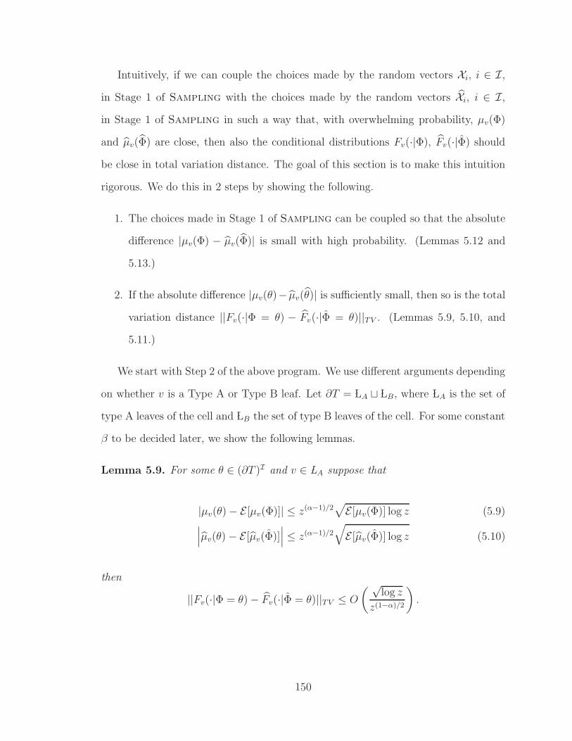
Intuitively, if we can couple the choices made by the random vectors Xi, i ∈ I,
in Stage 1 of Sampling with the choices made by the random vectors Xi, i ∈ I,
in Stage 1 of Sampling in such a way that, with overwhelming probability, µv(Φ)
and µv(Φ) are close, then also the conditional distributions Fv(·|Φ), Fv(·|Φ) should
be close in total variation distance. The goal of this section is to make this intuition
rigorous. We do this in 2 steps by showing the following.
1. The choices made in Stage 1 of Sampling can be coupled so that the absolute
difference |µv(Φ) − µv(Φ)| is small with high probability. (Lemmas 5.12 and
5.13.)
2. If the absolute difference |µv(θ)− µv(θ)| is sufficiently small, then so is the total
variation distance ||Fv(·|Φ = θ) − Fv(·|Φ = θ)||TV . (Lemmas 5.9, 5.10, and
5.11.)
We start with Step 2 of the above program. We use different arguments depending
on whether v is a Type A or Type B leaf. Let ∂T = LA ⊔ LB, where LA is the set of
type A leaves of the cell and LB the set of type B leaves of the cell. For some constant
β to be decided later, we show the following lemmas.
Lemma 5.9. For some θ ∈ (∂T )I and v ∈ LA suppose that
|µv(θ) − E [µv(Φ)]| ≤ z(α−1)/2√
E [µv(Φ)] log z (5.9)∣∣∣µv(θ) − E [µv(Φ)]
∣∣∣ ≤ z(α−1)/2
√E [µv(Φ)] log z (5.10)
then
||Fv(·|Φ = θ) − Fv(·|Φ = θ)||TV ≤ O
( √log z
z(1−α)/2
).
150
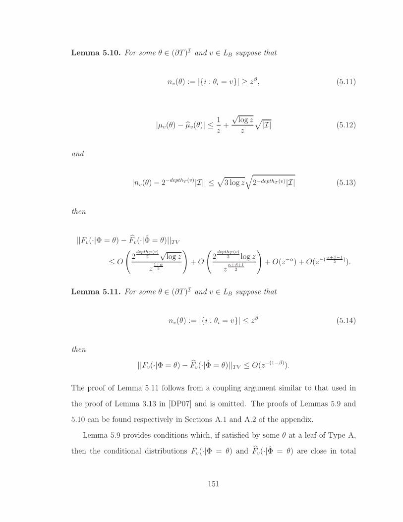
Lemma 5.10. For some θ ∈ (∂T )I and v ∈ LB suppose that
nv(θ) := |i : θi = v| ≥ zβ , (5.11)
|µv(θ) − µv(θ)| ≤ 1
z+
√log z
z
√|I| (5.12)
and
|nv(θ) − 2−depthT (v)|I|| ≤√
3 log z√
2−depthT (v)|I| (5.13)
then
||Fv(·|Φ = θ) − Fv(·|Φ = θ)||TV
≤ O
(2
depthT (v)
2
√log z
z1+α
2
)+ O
(2
depthT (v)
2 log z
zα+β+1
2
)+ O(z−α) + O(z−(α+β−1
2)).
Lemma 5.11. For some θ ∈ (∂T )I and v ∈ LB suppose that
nv(θ) := |i : θi = v| ≤ zβ (5.14)
then
||Fv(·|Φ = θ) − Fv(·|Φ = θ)||TV ≤ O(z−(1−β)).
The proof of Lemma 5.11 follows from a coupling argument similar to that used in
the proof of Lemma 3.13 in [DP07] and is omitted. The proofs of Lemmas 5.9 and
5.10 can be found respectively in Sections A.1 and A.2 of the appendix.
Lemma 5.9 provides conditions which, if satisfied by some θ at a leaf of Type A,
then the conditional distributions Fv(·|Φ = θ) and Fv(·|Φ = θ) are close in total
151
variation distance. Similarly, Lemmas 5.10 and 5.11 provide conditions for the leaves
of Type B. The following lemmas state that these conditions are satisfied with high
probability. Their proof is given in Section A.3 of the appendix.
Lemma 5.12. Let v ∈ LA. Then
G
θ : |µv(θ) − E [µv(Φ)]| ≤√
log zz(1−α)/2
√E [µv(Φ)]
∧∣∣∣µv(θ) − E [µv(Φ)]
∣∣∣ ≤√
log zz(1−α)/2
√E [µv(Φ)]
≥ 1 − 4z−1/3. (5.15)
Lemma 5.13. Let v ∈ LB. Then
G
θ : |µv(θ) − µv(θ)| ≤ 1+
√|I| log z
z
∧ |nv(θ) − 2−depthT (v)|I|| ≤ √3 log z
√2−depthT (v)|I|
≥ 1 − 4
z1/2. (5.16)
Setting α = 35
and β = 45
and combining the above, we have that, regardless of
whether v ∈ LA or v ∈ LB,
G
(θ : ||Fv(·|Φ = θ) − Fv(·|Φ = θ)||TV ≤ O
(2k log z
z1/5
))≥ 1 − 4
z1/3,
where we used that depthT (v) ≤ k as implied by Claim 5.5.
5.8 Extensions
Returning to our algorithm (Theorem 5.1), there are several directions in which it
can be immediately generalized. To give an idea of the possibilities, let us define a
semi-anonymous game to be a game in which
• the players are partitioned into a fixed number of types;
• there is another partition of the players into an arbitrary number of disjoint
graphical games of size O(log n), where n is the total number of players, and
bounded degree called extended families;
152

and the utility of each player depends on (a) his/her own strategy; (b) the overall
number of other players of each type playing each strategy; and (c) it also depends,
in an arbitrary way, on the strategy choices of neighboring nodes in his/her own
extended family. The following result, which is only indicative of the applicability
of our approach, can be shown by extending the discretization method via dynamic
programming (details omitted):
Theorem 5.14. There is a PTAS for semi-anonymous games with a fixed number of
strategies.
5.9 Towards Efficient Polynomial-Time Approxi-
mation Schemes
The polynomial-time approximation scheme presented in the previous sections com-
putes an ǫ-Nash equilibrium of an anonymous game with n players and k strategies
in time
O(nf(k,ǫ)
),
where f is polynomial in 1ǫ, but super-exponential in k. Hence, despite its theoretical
efficiency for bounded ǫ and k, the algorithm is not efficient in practice. Even for
the simpler case of 2 strategies per player, a more efficient implementation of our
algorithm, given in [DP07], runs in time
O(nO(1/ǫ2)
),
which is still not practical.
So, are there more efficient algorithms for computing Nash equilibria in anonymous
games? In recent work [Das08], we present an efficient polynomial-time approximation
153

scheme for the case of two strategies per player, with running time
poly(n) · (1/ǫ)O(1/ǫ2) .
This scales with the number of players as a polynomial of fixed degree, independent
of ǫ. The improved running time is based on a better understanding of certain struc-
tural properties of approximate Nash equilibria. In particular, we show that, for any
integer z, there exists an ǫ-approximate Nash equilibrium with ǫ = O(1/z), in which
(a) either, at most z3 = O((1/ǫ)3) players use randomized strategies, and their
strategies are integer multiples of 1/z2; 10
(b) or, all players who randomize choose the same mixed strategy which is an integer
multiple of 1zn
.
To derive the above characterization, we study mixed strategy profiles in the neigh-
borhood of a Nash equilibrium. We establish that there always exists a mixed strategy
profile in this neighborhood which is of one of the types (a) or (b) described above
and, moreover, satisfies the Nash equilibrium conditions to within an additive ǫ,
hence corresponding to an ǫ-approximate equilibrium. Given this structural result,
an ǫ-approximate equilibrium can be found by dynamic programming.
We feel that a more sophisticated analysis could establish similar structural prop-
erties for the approximate equilibria of multi-strategy anonymous games, thus ex-
tending our efficient PTAS to anonymous games with any fixed number of strategies.
Also, a more refined structural characterization of approximate Nash equilibria could
give more efficient algorithms, even a fully polynomial-time approximation scheme.
10Note that, since every player has 2 strategies, a mixed strategy is just a number in [0, 1].
154
Chapter 6
Conclusions and Open Problems
Motivated by the importance of Game Theory for the study of large systems of
strategic agents, such as the Internet, as well as social and biological systems, we
investigated whether Nash equilibria are efficiently computable. The significance of
this question is the following: The concept of the Nash equilibrium is one of Game
Theory’s most important frameworks for behavior prediction. For its predictions then
to be plausible it is crucial that it is efficiently computable; because, if it is not, it
would not be reasonable to expect that a group of strategic agents would be able to
discover it in every situation and behave as it prescribes.
Since by Nash’s theorem a Nash equilibrium is guaranteed to exist, to character-
ize the complexity of finding an equilibrium, we turned to the complexity theory of
total search problems in NP. For the case of two-player games, the Nash equilibrium
problem was known to belong to PPAD, defined to be the class of total search prob-
lems whose totality is certified by a parity argument in directed graphs [Pap94b].
We extended this result to all games; however, because in multi-player games all
equilibria may be irrational, we analyzed the problem of finding an ǫ-Nash equilib-
rium (for ǫ specified in the input), which we called Nash. Our main result was
that Nash is PPAD-complete. Since finding Brouwer fixed points of continuous and
155
piecewise-linear functions is also PPAD-complete [Pap94b], our result implies the
polynomial-time equivalence of these problems.
The class PPAD is not known to be inside P. Hence, our result raises questions
about the plausibility of the Nash equilibrium as a concept of behavior prediction.
To make this critique more solid, it is important to answer the following question.
• What is the true complexity of the class PPAD?
Showing P6=PPAD would imply that P6=NP, since PPAD is a subset of the search
problems in NP. Hence, a proof of this statement should involve major breakthroughs
in complexity theory. Therefore, a less ambitious goal would be to provide condi-
tional hardness results for the complexity of PPAD, possibly under cryptographic
assumptions such as the hardness of factoring an integer. In view of Shor’s algorithm
for factoring [Sho97] a reduction in the opposite direction would imply an interesting
(conditional) separation between deterministic and quantum polynomial time. In the
same spirit, it is interesting to investigate the following.
• What is the relation of PPAD to other classes at the boundary of P and NP and
to problems in cryptography?
Apart from the parity argument in directed graphs giving rise to the class PPAD, there
are several other (non-constructive) arguments for showing existence in combinatorics.
And, as discussed in Chapter 1, each of these arguments naturally defines a class
of total search problems in NP. The ones considered by Papadimitriou in [Pap94b]
include the existence of sinks in DAGs (which corresponds to the class PLS), the
pigeonhole principle (which gives rise to the class PPP), and the parity argument
on undirected graphs (which defines the class PPA). The complexity classes thus
defined provide a rich framework for characterizing the computational hardness of
total search problems in NP and may also be helpful for the systematic classification of
cryptographic problems. After all, most cryptographic primitives, such as the prime
156
factorization, the discrete logarithm, and the existence of short vectors in lattices,
correspond to total search problems. Evidence of hardness for these problems could
be of great significance for cryptography. For an extensive discussion of this point,
see, e.g., the work of Ajtai [Ajt96], where also lattice problems are defined from non-
constructive existence arguments in PPP; unfortunately, none of these arguments are
known to be PPP-complete.
Our PPAD-completeness result for the Nash equilibrium problem is a worst-case
result. But it could be the case that it does not apply for “situations arising in
practice.” To understand whether this is the case, we should investigate the following.
• Are there broad and important classes of games for which Nash equilibria can be
computed efficiently?
• Are there natural random ensembles of games for which the Nash equilibrium
problem is tractable with high probability?
As discussed in previous chapters, two-player zero-sum games are solvable exactly
in polynomial time [Neu28, Dan63, Kha79], and these are essentially the only in-
teresting games for which strong tractability results are known. For several other
special classes of games, such as win-lose games and two-player symmetric games,
intractability persists (see Section 4.3). An intriguing open problem at the boundary
of intractability is the following.
• What is the complexity of three-player symmetric games?
In the realm of random ensembles, Barany, Vempala and Vetta describe a simple
distribution over two-player games that can be solved exactly in polynomial time
with high probability [BVV07]. However, their ensemble — assuming that every
utility value is independently and identically distributed with respect to the others —
is rather special. On the other hand, finding a Nash equilibrium in the smoothed
157

complexity model (whereby every entry of the input game is perturbed with random
noise) is still PPAD-complete [CDT06a]. Whether there are natural and practically
appealing random ensembles of games for which the Nash equilibrium problem is
tractable remains an important open problem.
Shifting away from exact computation, we discussed in Chapter 5 that comput-
ing ǫ-Nash equilibria for values of ǫ scaling inverse-polynomially in the size of the
game remains PPAD-complete [CDT06a]; hence a fully polynomial-time approxima-
tion scheme is out of the question unless PPAD is equal to P. At the boundary of
intractability, the following emerges as an important open problem.
• Is there a polynomial-time approximation scheme for the Nash equilibrium problem?
Despite much research on the subject, the question remains open even for the case
of two-player games. In Chapter 5, we discussed special classes of two-player games for
which a PTAS exists, such as low-rank games and bounded-norm games. It is impor-
tant to consider the general case, as well as special classes for which a polynomial-time
approximation scheme exists. It is also important to consider whether polynomial-
time approximation schemes exist for graphical games. In [DP06], we describe a
polynomial-time approximation scheme for normalized graphical games with a con-
stant number of strategies per player, bounded degree, and treewidth which is at most
logarithmic in the number of players. Going beyond logarithmic treewidth would be
rather important.
• Is there a polynomial-time approximation scheme for graphical games of bounded
degree, but super-logarithmic treewidth?
Another case worth studying is when the degree is super-logarithmic. In this
case, our PPAD-completeness result for graphical games does not apply. Is it then
the case that the problem is easier? In [DP08a], we show that an ǫ-Nash equilibrium
of a normalized normal-form game with two strategies per player can be computed
158

in time nO(log log n+log 1ǫ), where n is the size of the game. It is intriguing to examine if
this result can be improved.
• Is there a polynomial-time approximation scheme for multi-player normal-form
games with two strategies per player?
Finally, it is important to study other broad and important classes of games which
can be approximated efficiently. In Chapter 5, we considered anonymous games and
presented a polynomial-time approximation scheme for the case of many players and
a constant number of strategies per player. If the number of players is constant, and
the number of strategies scales, the problem becomes PPAD-complete. The following
questions arise.
• Is the Nash equilibrium problem in multi-player anonymous games with a constant
number of strategies per player PPAD-complete? More generally, what tradeoff be-
tween number of strategies and players renders the problem PPAD-complete?
• Does our PTAS for multi-player anonymous games extend to a super-constant
number of strategies per player?
• Is there a fully polynomial-time approximation scheme for multi-player anonymous
games with a constant number of strategies per player? If not, is there an efficient
PTAS?
In [Das08], we make progress towards answering the last question by providing an
efficient PTAS for the case of two-strategy anonymous games. We believe that our
techniques should extend to any constant number of strategies and could possibly also
provide a fully polynomial-time approximation scheme. Regarding the first couple of
questions, let us note that Papadimitriou and Roughgarden provide in [PR05] an
algorithm for multi-player symmetric games — a special case of anonymous games —
which remains efficient up to about a logarithmic number of strategies per player. We
believe that a similar result should be possible for anonymous games.
159
Bibliography
[Ajt96] Miklos Ajtai. Generating Hard Instances of Lattice Problems (Extended
Abstract). In the 28th Annual ACM Symposium on Theory of Computing
(STOC), 1996.
[AKV05] Timothy G. Abbott, Daniel Kane, and Paul Valiant. On the Complexity
of Two-Player Win-Lose Games. In the 46th Annual IEEE Symposium on
Foundations of Computer Science (FOCS), 2005.
[AR86] Donald J. Albers and Constance Reid. An Interview with George B.
Dantzig: The Father of Linear Programming. The College Mathematics
Journal, 17(4):293–314, 1986.
[AV07] Ilan Adler and Sushil Verma. The Linear Complementarity Prob-
lem, Lemke Algorithm, Perturbation, and the Complexity Class PPAD.
Manuscript, 2007.
[Bar05] Andrew D. Barbour. Multivariate Poisson-Binomial Approximation Using
Stein’s Method. A. D. Barbour and L. H. Y. Chen (editors), Lecture Notes
Series No. 4, Institute for Mathematical Sciences, National University of
Singapore, Singapore University Press and World Scientific, 2005.
160
[BBM07] Hartwig Bosse, Jaroslaw Byrka, and Evangelos Markakis. New Algorithms
for Approximate Nash Equilibria in Bimatrix Games. In the 3rd Interna-
tional Workshop on Internet and Network Economics (WINE), 2007.
[BC05] Andrew D. Barbour and Louis H. Y. Chen. An Introduction to Stein’s
Method. A. D. Barbour and L. H. Y. Chen (editors), Lecture Notes Se-
ries No. 4, Institute for Mathematical Sciences, National University of
Singapore, Singapore University Press and World Scientific, 2005.
[BCE+98] Paul Beame, Stephen A. Cook, Jeff Edmonds, Russell Impagliazzo, and
Toniann Pitassi. The Relative Complexity of NP Search Problems. Journal
of Computer and System Sciences, 57(1):3–19, 1998.
[BCI+08] Christian Borgs, Jennifer T. Chayes, Nicole Immorlica, Adam Tauman
Kalai, Vahab S. Mirrokni, and Christos H. Papadimitriou. The Myth of
the Folk Theorem. In the 40th Annual ACM Symposium on Theory of
Computing (STOC), 2008.
[Bha75] Rabindra N. Bhattacharya. On Errors of Normal Approximation. The
Annals of Probability, 3(5):815–828, 1975.
[BHJ92] Andrew D. Barbour, Lars Holst, and Svante Janson. Poisson Approxima-
tion. Oxford University Press, 1992.
[BL06] Andrew D. Barbour and Torgny Lindvall. Translated Poisson Approxima-
tion for Markov Chains. Journal of Theoretical Probability, 19(3):609–630,
2006.
[Blo99] Matthias Blonski. Anonymous Games with Binary Actions. Games and
Economic Behavior, 28(2):171–180, 1999.
161
[Blo05] Matthias Blonski. The Women of Cairo: Equilibria in Large Anonymous
Games. Journal of Mathematical Economics, 41(3):253–264, 2005.
[BN50] George W. Brown and John von Neumann. Solutions of Games by Differ-
ential Equations. In H. W. Kuhn and A. W. Tucker (editors), Contribu-
tions to the Theory of Games, volume 1, pages 73–79. Princeton University
Press, 1950.
[Bub79] Valentinas Bubelis. On Equilibria in Finite Games. International Journal
of Game Theory, 8(2):65–79, 1979.
[BVV07] Imre Barany, Santosh Vempala, and Adrian Vetta. Nash equilibria in
random games. Random Structures and Algorithms, 31(4):391–405, 2007.
[CD05] Xi Chen and Xiaotie Deng. 3-Nash is PPAD-Complete. Electronic Collo-
quium on Computational Complexity (ECCC), (134), 2005.
[CD06] Xi Chen and Xiaotie Deng. Settling the Complexity of Two-Player Nash
Equilibrium. In the 47th Annual IEEE Symposium on Foundations of
Computer Science (FOCS), 2006.
[CDT06a] Xi Chen, Xiaotie Deng, and Shang-Hua Teng. Computing Nash Equilib-
ria: Approximation and Smoothed Complexity. In the 47th Annual IEEE
Symposium on Foundations of Computer Science (FOCS), 2006.
[CDT06b] Xi Chen, Xiaotie Deng, and Shang-Hua Teng. Sparse Games Are Hard.
In the 2nd International Workshop on Internet and Network Economics
(WINE), 2006.
[CKK+00] Gerard J. Chang, Wen-Tsai Ke, David Kuo, Daphne Der-Fen Liu, and
Roger K. Yeh. On l(d, 1)-Labelings of Graphs. Discrete Mathematics,
220(1-3):57–66, 2000.
162

[Con92] Anne Condon. The Complexity of Stochastic Games. Information and
Computation, 96(2):203–224, 1992.
[CS03] Vincent Conitzer and Tuomas Sandholm. Complexity Results about Nash
Equilibria. In the 18th International Joint Conference on Artificial Intel-
ligence (IJCAI), 2003.
[CSVY06] Bruno Codenotti, Amin Saberi, Kasturi R. Varadarajan, and Yinyu Ye.
Leontief Economies Encode Nonzero Sum Two-Player Games. In the 17th
Annual ACM-SIAM Symposium on Discrete Algorithms (SODA), 2006.
[CT06] Thomas M. Cover and Joy A. Thomas. Elements of Information Theory.
Wiley, 2006.
[CTV07] Xi Chen, Shang-Hua Teng, and Paul Valiant. The Approximation Com-
plexity of Win-Lose Games. In the 18th Annual ACM-SIAM Symposium
on Discrete Algorithms (SODA), 2007.
[Dan63] George B. Dantzig. Linear Programming and Extensions. Princeton Uni-
versity Press, 1963.
[Das08] Constantinos Daskalakis. An Efficient PTAS for Two-Strategy Anony-
mous Games. Manuscript, 2008.
[DFP06] Constantinos Daskalakis, Alex Fabrikant, and Christos H. Papadimitriou.
The Game World Is Flat: The Complexity of Nash Equilibria in Succinct
Games. In the 33rd International Colloquium on Automata, Languages
and Programming (ICALP), 2006.
[DGP06] Constantinos Daskalakis, Paul W. Goldberg, and Christos H. Papadim-
itriou. The Complexity of Computing a Nash Equilibrium. In the 38th
Annual ACM Symposium on Theory of Computing (STOC), 2006.
163
[DMP06] Constantinos Daskalakis, Aranyak Mehta, and Christos H. Papadimitriou.
A Note on Approximate Nash Equilibria. In the 2nd International Work-
shop on Internet and Network Economics (WINE), 2006.
[DMP07] Constantinos Daskalakis, Aranyak Mehta, and Christos H. Papadimitriou.
Progress in Approximate Nash Equilibria. In 8th ACM Conference on
Electronic Commerce (EC), 2007.
[DP05] Constantinos Daskalakis and Christos H. Papadimitriou. Three-Player
Games Are Hard. Electronic Colloquium on Computational Complexity
(ECCC), (139), 2005.
[DP06] Constantinos Daskalakis and Christos H. Papadimitriou. Computing Pure
Nash Equilibria in Graphical Games via Markov Random Fields. In the
7th ACM Conference on Electronic Commerce (EC), 2006.
[DP07] Constantinos Daskalakis and Christos H. Papadimitriou. Computing
Equilibria in Anonymous Games. In the 48th Annual IEEE Symposium
on Foundations of Computer Science (FOCS), 2007.
[DP08a] Constantinos Daskalakis and Christos H. Papadimitriou. Discretized
Multinomial Distributions and Nash Equilibria in Anonymous Games. In
the 49th Annual IEEE Symposium on Foundations of Computer Science
(FOCS), 2008.
[DP08b] Constantinos Daskalakis and Christos H. Papadimitriou. On Oblivious
PTAS for Nash Equilibrium. Manuscript, 2008.
[Eav72] B. Curtis Eaves. Homotopies for Computation of Fixed Points. Mathe-
matical Programming, 3:1–22, 1972.
164

[EGG06] Edith Elkind, Leslie Ann Goldberg, and Paul W. Goldberg. Nash Equi-
libria in Graphical Games on Trees Revisited. In the 7th ACM Conference
on Electronic Commerce (EC), 2006.
[EY07] Kousha Etessami and Mihalis Yannakakis. On the Complexity of Nash
Equilibria and Other Fixed Points (Extended Abstract). In the 48th
Annual IEEE Symposium on Foundations of Computer Science (FOCS),
2007.
[FL99] Drew Fudenberg and David K. Levine. The Theory of Learning in Games.
The MIT Press, 1999.
[FNS07] Tomas Feder, Hamid Nazerzadeh, and Amin Saberi. Approximating Nash
Equilibria Using Small-Support Strategies. In the 8th ACM Conference
on Electronic Commerce (EC), 2007.
[FPT04] Alex Fabrikant, Christos H. Papadimitriou, and Kunal Talwar. The Com-
plexity of Pure Nash Equilibria. In the 36th Annual ACM Symposium on
Theory of Computing (STOC), 2004.
[G91] Friedrich Gotze. On the Rate of Convergence in the Multivariate CLT.
The Annals of Probability, 19(2):724–739, 1991.
[GGJ76] M. R. Garey, Ronald L. Graham, and David S. Johnson. Some NP-
Complete Geometric Problems. In the 8th Annual ACM Symposium on
Theory of Computing (STOC), 1976.
[GKT50] David Gale, Harold W. Kuhn, and Albert W. Tucker. On Symmetric
Games. In H. W. Kuhn and A. W. Tucker (editors), Contributions to
the Theory of Games, volume 1, pages 81–87. Princeton University Press,
1950.
165
[GLL73] Crisostomo B. Garcia, Carlton E. Lemke, and Hans-Jakob Luthi. Simpli-
cial Approximation of an Equilibrium Point of Noncooperative N-Person
Games. Mathematical Programming, 4:227–260, 1973.
[GP06] Paul W. Goldberg and Christos H. Papadimitriou. Reducibility Among
Equilibrium Problems. In the 38th Annual ACM Symposium on Theory
of Computing (STOC), 2006.
[GZ89] Itzhak Gilboa and Eitan Zemel. Nash and Correlated Equilibria: Some
Complexity Considerations. Games and Economic Behavior, 1(1):80–93,
1989.
[HPV89] Michael D. Hirsch, Christos H. Papadimitriou, and Stephen A. Vavasis.
Exponential Lower Bounds for Finding Brouwer Fixed Points. Journal of
Complexity, 5(4):379–416, 1989.
[JPY88] David S. Johnson, Christos H. Papadimitriou, and Mihalis Yannakakis.
How Easy is Local Search? Journal of Computer and System Sciences,
37(1):79–100, 1988.
[Kal05] Ehud Kalai. Partially-Specified Large Games. In the 1st International
Workshop on Internet and Network Economics (WINE), 2005.
[Kha79] Leonid G. Khachiyan. A Polynomial Algorithm in Linear Programming.
Soviet Mathematics Doklady, 20(1):191–194, 1979.
[KKM29] Bronislaw Knaster, Casimir Kuratowski, and Stefan Mazurkiewicz. Ein
Beweis des Fixpunktsatzes fur n-dimensionale Simplexe. Fundamenta
Mathematicae, 14:132–137, 1929.
166
[KLS01] Michael J. Kearns, Michael L. Littman, and Satinder P. Singh. Graphi-
cal Models for Game Theory. In the 17th Conference in Uncertainty in
Artificial Intelligence (UAI), 2001.
[KPS06] Spyros C. Kontogiannis, Panagiota N. Panagopoulou, and Paul G. Spi-
rakis. Polynomial Algorithms for Approximating Nash Equilibria of Bima-
trix Games. In the 2nd International Workshop on Internet and Network
Economics (WINE), 2006.
[KT07] Ravi Kannan and Thorsten Theobald. Games of Fixed Rank: a Hierar-
chy of Bimatrix Games. In the 18th Annual ACM-SIAM Symposium on
Discrete Algorithms (SODA), 2007.
[LH64] Carlton E. Lemke and Joseph T. Howson, Jr. Equilibrium Points of Bima-
trix Games. Journal of the Society for Industrial and Applied Mathematics,
12(2):413–423, 1964.
[LM04] Richard J. Lipton and Evangelos Markakis. Nash Equilibria via Polyno-
mial Equations. In 6th Latin American Symposium (LATIN), 2004.
[LMM03] Richard J. Lipton, Evangelos Markakis, and Aranyak Mehta. Playing
Large Games Using Simple Strategies. In the 4th ACM Conference on
Electronic Commerce (EC), 2003.
[LT79] Gerard van der Laan and Adolphus Johannes Jan Talman. A Restart Al-
gorithm for Computing Fixed Points Without an Extra Dimension. Math-
ematical Programming, 17(1):74–84, 1979.
[LT82] Gerard van der Laan and Adolphus Johannes Jan Talman. On the Com-
putation of Fixed Points in the Product Space of Unit Simplices and an
167
Application to Noncooperative N Person Games. Mathematics of Opera-
tions Research, 7(1):1–13, 1982.
[Mil96] Igal Milchtaich. Congestion Games with Player-Specific Payoff Functions.
Games and Economic Behavior, 13:111–124, 1996.
[MP91] Nimrod Megiddo and Christos H. Papadimitriou. On Total Functions, Ex-
istence Theorems and Computational Complexity. Theoretical Computer
Science, 81(2):317–324, 1991.
[Nas51] John Nash. Non-Cooperative Games. Annals of Mathematics, 54(2):286–
295, 1951.
[Neu28] John von Neumann. Zur Theorie der Gesellshaftsspiele. Mathematische
Annalen, 100:295–320, 1928.
[NM44] John von Neumann and Oskar Morgenstern. Theory of Games and Eco-
nomic Behavior. Princeton University Press, 1944.
[OR94] Martin J. Osborne and Ariel Rubinstein. A Course in Game Theory. MIT
Press, 1994.
[Pap77] Christos H. Papadimitriou. The Euclidean Traveling Salesman Problem
is NP-Complete. Theoretical Computer Science, 4(3):237–244, 1977.
[Pap94a] Christos H. Papadimitriou. Computational Complexity. Addison-Wesley,
1994.
[Pap94b] Christos H. Papadimitriou. On the Complexity of the Parity Argument
and Other Inefficient Proofs of Existence. Journal of Computer and System
Sciences, 48(3):498–532, 1994.
168

[PR05] Christos H. Papadimitriou and Tim Roughgarden. Computing Equilibria
in Multi-Player Games. In the 16th Annual ACM-SIAM Symposium on
Discrete Algorithms (SODA), pages 82–91, 2005.
[R07] Adrian Rollin. Translated Poisson Approximation Using Exchangeable
Pair Couplings. Annals of Applied Probability, 17:1596–1614, 2007.
[Roo98] Bero Roos. Metric Multivariate Poisson Approximation of the General-
ized Multinomial Distribution. Theory of Probability and its Applications,
43(2):306–315, 1998.
[Ros71] Joachim Rosenmuller. On a Generalization of the Lemke-Howson Algo-
rithm to Noncooperative N-Person Games. SIAM Journal on Applied
Mathematics, 21(1):73–79, 1971.
[Ros73] Robert W. Rosenthal. A Class of Games Possessing Pure-Strategy Nash
Equilibria. International Journal of Game Theory, 2(1):65–67, 1973.
[Rub79] Ariel Rubinstein. Equilibrium in Supergames with the Overtaking Crite-
rion. Journal of Economic Theory, 21:1–9, 1979.
[Sca67] Herbert E. Scarf. The Approximation of Fixed Points of a Continuous
Mapping. SIAM Journal on Applied Mathematics, 15(5):1328–1343, 1967.
[Sho97] Peter Shor. Polynomial-Time Algorithms for Prime Factorization and Dis-
crete Logarithms on a Quantum Computer. SIAM Journal of Computing,
26(5):1484–1509, 1997.
[SS04] Rahul Savani and Bernhard von Stengel. Exponentially Many Steps for
Finding a Nash Equilibrium in a Bimatrix Game. In the 45th Symposium
on Foundations of Computer Science (FOCS), 2004.
169
[SV06] Grant Schoenebeck and Salil P. Vadhan. The Computational Complexity
of Nash Equilibria in Concisely Represented Games. In the 7th ACM
Conference on Electronic Commerce (EC), 2006.
[TS07] Haralampos Tsaknakis and Paul G. Spirakis. An Optimization Approach
for Approximate Nash Equilibria. In the 3rd International Workshop on
Internet and Network Economics (WINE), 2007.
[Wil71] Robert Wilson. Computing Equilibria of N-Person Games. SIAM Journal
on Applied Mathematics, 21(1):80–87, 1971.
170
Appendix A
Skipped Proofs
Proof of Claim 5.5: That a tree resulting from TDP has k − 1 leaves follows by
induction: It is true when k = 2, and for general k, the left subtree has j strategies
and thus, by induction, j − 1 leaves, and the right subtree has at most k + 1 − j
strategies and k − j leaves; adding we get the result.
To estimate the number of cells, let us fix the set of strategies and their ordering
at the root of the tree (thus the result of the calculation will have to be multiplied
by 2kk!) and then count the number of trees that could be output by TDP. Suppose
that the root has cardinality m and that the children of the root are assigned sets of
sizes j and m+1− j (or, in the event of no duplication, m− j), respectively. If j = 2,
then a duplication has to have happened and, for the ordering of the strategies at
the left child of the root, there are at most 2 possibilities depending on whether the
“divided strategy” is still the largest at the left side; similarly, for the right side there
are m−1 possibilities: either the divided strategy is still the largest at the right side,
or it is not in which case it has to be inserted at the correct place in the ordering
and the last strategy of the right side must be moved to the second place. If j > 2,
similar considerations show that there are at most j − 1 possibilities for the left side
and 1 possibility for the right side. It follows that the number of trees is bounded
171
from above by the solution T (k) of the recurrence
T (n) = 2 T (2) · (n − 1)T (n − 1)
+
n−1∑
j=3
(j − 1)T (j) · maxT (n − j), T (n + 1 − j).
with T(2)=1. It follows that the total number of trees can be upper-bounded by the
function kk2. Taking into account that there are 2kk! choices for the set of strategies
and their ordering at the root of the tree, and that each leaf can be of either Type A, or
of Type B, it follows that the total number of cells is bounded by g(k) = kk22k−12kk!.
2
Proof of Claim 5.6: The proof follows by a straightforward coupling argument.
Indeed, for all i ∈ I, let us couple the choices made by Stage 1 of Sampling Xi
and Sampling Xi so that the random leaf Φi ∈ ∂T chosen by Sampling Xi and
the random leaf Φi ∈ ∂T chosen by Sampling Xi are equal, that is, for all i ∈ I,
in the joint probability space Pr[Φi = Φi] = 1; the existence of such a coupling is
straightforward since Stage 1 of both Sampling Xi and Sampling Xi is the same
random walk on T . 2
Proof of Lemma 5.8: Let us denote by
Good = θ|θ ∈ (∂T )I : ||F (·|Φ = θ) − F (·|Φ = θ)||TV ≤ O
(k
2k log z
z1/5
),
and let Bad = (∂T )I −Good. By Equation (5.7) if follows that G(Bad) ≤ O(kz−1/3).
172
||T − T ||TV =1
2
∑
t
|F (t) − F (t)|
=1
2
∑
t
∣∣∣∣∣∑
θ
F (t|Φ = θ)G(Φ = θ) −∑
θ
F (t|Φ = θ)G(Φ = θ)
∣∣∣∣∣
=1
2
∑
t
∣∣∣∣∣∑
θ
(F (t|Φ = θ) − F (t|Φ = θ))G(θ)
∣∣∣∣∣(
using G(θ) = G(θ), ∀θ)
≤ 1
2
∑
t
∑
θ
∣∣∣F (t|Φ = θ) − F (t|Φ = θ)∣∣∣G(θ)
=1
2
∑
t
∑
θ∈Good
∣∣∣F (t|Φ = θ) − F (t|Φ = θ)∣∣∣G(θ)
+1
2
∑
t
∑
θ∈Bad
∣∣∣F (t|Φ = θ) − F (t|Φ = θ)∣∣∣G(θ)
≤∑
θ∈Good
G(θ)
(1
2
∑
t
∣∣∣F (t|Φ = θ) − F (t|Φ = θ)∣∣∣)
+∑
θ∈Bad
G(θ)
(1
2
∑
t
∣∣∣F (t|Φ = θ) − F (t|Φ = θ)∣∣∣)
≤∑
θ∈Good
G(θ) · O(
k2k log z
z1/5
)+∑
θ∈Bad
G(θ)
≤ O
(k
2k log z
z1/5
)+ O(kz−1/3).
2
A.1 Proof of Lemma 5.9
Proof. By the assumption it follows that
|µv(θ) − µv(θ)| ≤∣∣∣E [µv(Φ)] − E [µv(Φ)]
∣∣∣ + z(α−1)/2√E [µv(Φ)] log z + z(α−1)/2
√E [µv(Φ)] log z.
173
Moreover, note that
E [µv(Φ)] = 2−depthT (v)∑
i∈Ipi,v(ℓ∗v)
and, similarly,
E [µv(Φ)] = 2−depthT (v)∑
i∈Ipi,v(ℓ∗v).
By the definition of the Rounding procedure it follows that
|E [µv(Φ)] − E [µv(Φ)]| ≤ 2−depthT (v) 1
z.
Hence it follows that
|µv(θ) − µv(θ)| ≤ 2−depthT (v) 1
z+
2√
log z
z(1−α)/2
√max E [µv(Φ), E [µv(Φ)]]. (A.1)
Let Nv(θ) := i : θi = v, nv = |Nv|. Conditioned on Φ = θ, the distribution of
Tv,1 is the sum of nv independent Bernoulli random variables Zii∈Nv with expecta-
tions E [Zi] = pi,v(ℓ∗v) ≤ ⌊zα⌋z
. Similarly, conditioned on Φ = θ, the distribution of Tv,1
is the sum of nv independent Bernoulli random variables Zii∈Nv with expectations
E [Zi] = pi,v(ℓ∗v) ≤ ⌊zα⌋z
. Note that
E[∑
i∈Nv
Zi
]= µv(θ)
and, similarly,
E[∑
i∈Nv
Zi
]= µv(θ).
Without loss of generality, let us assume that E [µv(Φ)] ≥ E [µv(Φ)]. Let us further
174
distinguish two cases for some constant τ < 1 − α to be decided later
Case 1: E [µv(Φ)] ≤ 1zτ .
From (5.9) it follows that,
µv(θ) ≤ E [µv(Φ)] + z(α−1)/2√E [µv(Φ)] log z ≤ 1
zτ+
√log z
z(τ+1−α)/2=: g(z).
Similarly, because E [µv(Φ)] ≤ E [µv(Φ)] ≤ 1zτ , µv(θ) ≤ g(z).
By Markov’s inequality, PrΦ=θ[∑
i∈NvZi ≥ 1] ≤ µv(θ)
1≤ g(z) and, similarly,
PrΦ=θ[∑
i∈NvZi ≥ 1] ≤ g(z). Hence,
∣∣∣∣∣Pr Φ=θ
[∑
i∈Nv
Zi = 0
]− Pr Φ=θ
[∑
i∈Nv
Zi = 0
]∣∣∣∣∣
=
∣∣∣∣∣Pr Φ=θ
[∑
i∈Nv
Zi ≥ 1
]− Pr Φ=θ
[∑
i∈Nv
Zi ≥ 1
]∣∣∣∣∣ ≤ 2g(z).
It then follows easily that
||Fv(·|Φ = θ) − Fv(·|Φ = θ)||TV ≤ 4g(z) = 4 ·(
1
zτ+
√log z
z(τ+1−α)/2
). (A.2)
Case 2: E [µv(Φ)] ≥ 1zτ .
The following claim was proven in [DP07] (Lemma 3.9).
Claim A.1. For any set of independent Bernoulli random variables Zii with ex-
pectations E [Zi] ≤ ⌊zα⌋z
,
∥∥∥∥∥∑
i
Zi − Poisson
(E(∑
i
Zi
))∥∥∥∥∥TV
≤ 1
z1−α.
175
By application of this lemma it follows that
∥∥∥∥∥∑
i∈Nv
Zi − Poisson(µv(θ))
∥∥∥∥∥TV
≤ 1
z1−α, (A.3)
∥∥∥∥∥∑
i∈Nv
Zi − Poisson(µv(θ))
∥∥∥∥∥TV
≤ 1
z1−α. (A.4)
We study next the distance between the two Poisson distributions. We use the fol-
lowing lemma whose proof is postponed till later in this section.
Lemma A.2. If λ = λ0 + D for some D > 0, λ0 > 0,
‖Poisson(λ) − Poisson(λ0)‖TV ≤ D
√2
λ0
.
An application of Lemma A.2 gives
‖Poisson(µv(θ)) − Poisson(µv(θ))‖TV ≤ |µv(θ) − µv(θ)|√
2
min µv(θ), µv(θ) .
(A.5)
We conclude with the following lemma proved in the end of this section.
Lemma A.3. From (5.9), (5.10), (A.1) and the assumption E [µv(Φ)] ≥ 1zτ , it follows
that
|µv(θ) − µv(θ)|√
2
min µv(θ), µv(θ) ≤√
72log z
z1−α.
Combining (A.3), (A.4), (A.5) and Lemma A.3 we get
∥∥∥∥∥∑
i∈Nv
Zi −∑
i∈Nv
Zi
∥∥∥∥∥TV
≤ 2
z1−α+
√72
log z
z1−α= O
( √log z
z(1−α)/2
),
176
which implies
||Fv(·|Φ = θ) − Fv(·|Φ = θ)||TV ≤ O
( √log z
z(1−α)/2
). (A.6)
Taking τ > (1 − α)/2, we get from (A.2), (A.6) that in both cases
||Fv(·|Φ = θ) − Fv(·|Φ = θ)||TV ≤ O
( √log z
z(1−α)/2
). (A.7)
Proof of lemma A.2: We make use of the following lemmas.
Lemma A.4. If λ, λ0 > 0, the Kullback-Leibler divergence between Poisson(λ0) and
Poisson(λ) is given by
∆KL(Poisson(λ)||Poisson(λ0)) = λ
(1 − λ0
λ+
λ0
λlog
λ0
λ
).
Lemma A.5 (e.g. [CT06]). If P and Q are probability measures on the same measure
space and P is absolutely continuous with respect to Q then
‖P − Q‖TV ≤√
2∆KL(P ||Q).
By simple calculus we have that
∆KL(Poisson(λ)||Poisson(λ0)) = λ
(1 − λ0
λ+
λ0
λlog
λ0
λ
)≤ D2
λ0
.
Then by Lemma A.5 it follows that
‖Poisson(λ) − Poisson(λ0)‖TV ≤ D
√2
λ0.
177

2
Proof of lemma A.3: From (A.1) and the assumption E [µv(Φ)] ≥ E [µv(Φ)] we
have
|µv(θ) − µv(θ)|2 ≤ 1
z2+
4 log z
z1−αE [µv(Φ)] + 4
1
z
√log z
z(1−α)/2
√E [µv(Φ)].
From the assumption E [µv(Φ)] ≥ 1zτ it follows
E [µv(Φ)] =√
E [µv(Φ)]√
E [µv(Φ)] (A.8)
≥ 1
zτ/2
√E [µv(Φ)]. (A.9)
Since τ < 1 − α, it follows that, for sufficiently large z which only depends on α and
τ , 1zτ/2 ≥ 2
√log z
z(1−α)/2 . Hence,
E [µv(Φ)] ≥ 2√
log z
z(1−α)/2
√E [µv(Φ)],
which together with (5.9) implies
µv(θ) ≥ E [µv(Φ)] − z(α−1)/2√E [µv(Φ)] log z ≥ 1
2E [µv(Φ)] (A.10)
Similarly, starting from E [µv(Φ)] ≥ E [µv(Φ)] − 1z≥ 1
zτ − 1z, it can be shown that for
sufficiently large z
µv(θ) ≥ 1
2E [µv(Φ)]. (A.11)
From (A.10), (A.11) it follows that
minµv(θ), µv(θ) ≥ 1
2minE [µv(Φ)], E [µv(Φ)] =
1
2E [µv(Φ)] ≥ 1
2E [µv(Φ)] − 1
2z≥ 1
4E [µv(Φ)],
178
where we used that E [µv(Φ)] ≥ 1zτ ≥ 2
zfor sufficiently large z, since τ < 1 − α.
Combining the above we get
2|µv(θ) − µv(θ)|2min µv(θ), µv(θ) ≤ 2
1z2 + 4 log z
z1−α E [µv(Φ)] + 41z
√log z
z(1−α)/2
√E [µv(Φ)]
14E [µv(Φ)]
≤ 81
z2E [µv(Φ)]+ 32
log z
z1−α+ 32
√log z
z1+(1−α)/2√E [µv(Φ)]
≤ 8zτ
z2+ 32
log z
z1−α+ 32
zτ/2√
log z
z1+(1−α)/2
≤ 81
z2−τ+ 32
log z
z1−α+ 32
√log z
z(3−α−τ)/2
≤ 72log z
z1−α,
since 2 − τ > 1 − α and (3 − α − τ)/2 > 1 − α, assuming sufficiently large z. 2
A.2 Proof of Lemma 5.10
Proof. We will derive our bound by approximating with the translated Poisson dis-
tribution, which is defined next.
Definition A.6 ([R07]). We say that an integer random variable Y has a translated
Poisson distribution with paremeters µ and σ2 and write
L(Y ) = TP (µ, σ2)
if L(Y −⌊µ−σ2⌋) = Poisson(σ2 +µ−σ2), where µ−σ2 represents the fractional
part of µ − σ2.
The following lemma provides a bound for the total variation distance between two
translated Poisson distributions with different parameters.
179
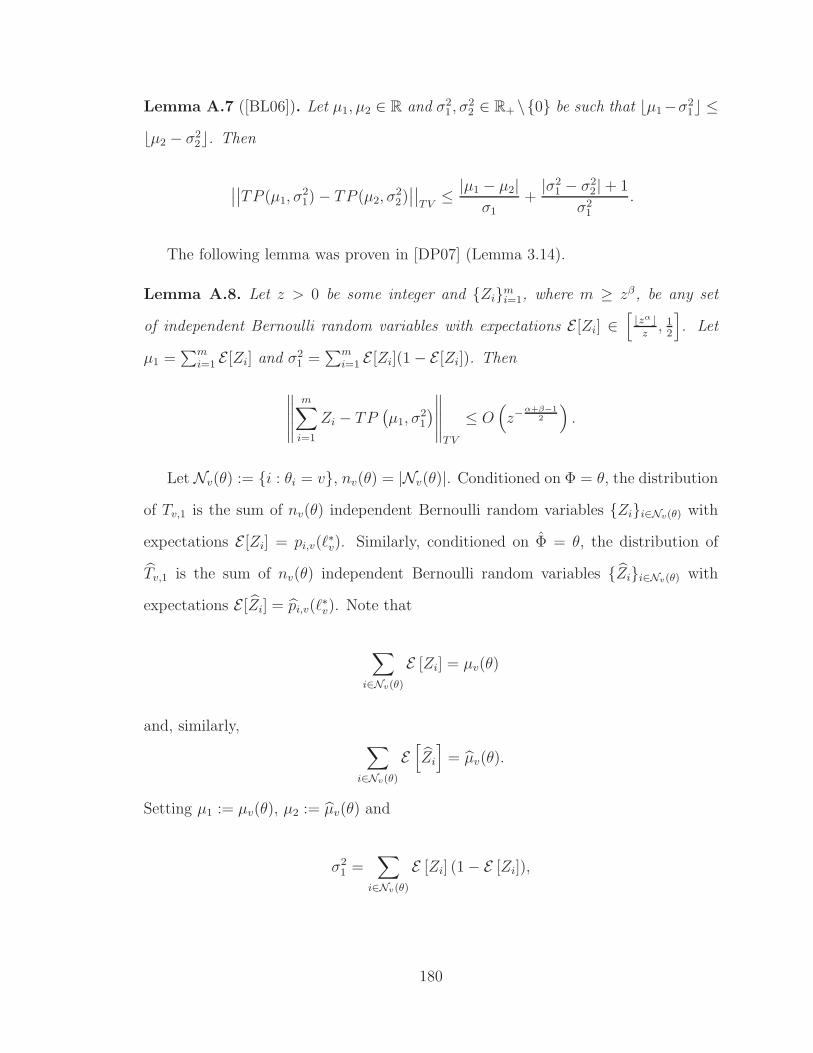
Lemma A.7 ([BL06]). Let µ1, µ2 ∈ R and σ21 , σ
22 ∈ R+ \0 be such that ⌊µ1−σ2
1⌋ ≤
⌊µ2 − σ22⌋. Then
∣∣∣∣TP (µ1, σ21) − TP (µ2, σ
22)∣∣∣∣
TV≤ |µ1 − µ2|
σ1+
|σ21 − σ2
2| + 1
σ21
.
The following lemma was proven in [DP07] (Lemma 3.14).
Lemma A.8. Let z > 0 be some integer and Zimi=1, where m ≥ zβ, be any set
of independent Bernoulli random variables with expectations E [Zi] ∈[⌊zα⌋
z, 1
2
]. Let
µ1 =∑m
i=1 E [Zi] and σ21 =
∑mi=1 E [Zi](1 − E [Zi]). Then
∥∥∥∥∥
m∑
i=1
Zi − TP(µ1, σ
21
)∥∥∥∥∥
TV
≤ O(z−
α+β−12
).
Let Nv(θ) := i : θi = v, nv(θ) = |Nv(θ)|. Conditioned on Φ = θ, the distribution
of Tv,1 is the sum of nv(θ) independent Bernoulli random variables Zii∈Nv(θ) with
expectations E [Zi] = pi,v(ℓ∗v). Similarly, conditioned on Φ = θ, the distribution of
Tv,1 is the sum of nv(θ) independent Bernoulli random variables Zii∈Nv(θ) with
expectations E [Zi] = pi,v(ℓ∗v). Note that
∑
i∈Nv(θ)
E [Zi] = µv(θ)
and, similarly,∑
i∈Nv(θ)
E[Zi
]= µv(θ).
Setting µ1 := µv(θ), µ2 := µv(θ) and
σ21 =
∑
i∈Nv(θ)
E [Zi] (1 − E [Zi]),
180

σ22 =
∑
i∈Nv(θ)
E[Zi
](1 − E
[Zi
]),
we have from Lemma A.8 that
∥∥∥∥∥∥
∑
i∈Nv(θ)
Zi − TP(µ1, σ
21
)∥∥∥∥∥∥
TV
≤ O(z−
α+β−12
). (A.12)
∥∥∥∥∥∥
∑
i∈Nv(θ)
Zi − TP(µ2, σ
22
)∥∥∥∥∥∥
TV
≤ O(z−
α+β−12
). (A.13)
It remains to bound the total variation distance between the translated poisson dis-
tributions using Lemma A.7. Without loss of generality let us assume ⌊µ1 − σ21⌋ ≤
⌊µ2 − σ22⌋. Note that
σ21 =
∑
i∈Nv(θ)
E [Zi] (1 − E [Zi]) ≥ nv(θ)⌊zα⌋
z
(1 − ⌊zα⌋
z
)≥ 1
2nv(θ)
⌊zα⌋z
,
where the last inequality holds for values of z which are larger than some function of
constant α. Also,
|σ21 − σ2
2 | ≤∑
i∈Nv(θ)
∣∣∣E [Zi] (1 − E [Zi]) − E[Zi
](1 − E
[Zi
])∣∣∣
=∑
i∈Nv(θ)
|pi,v(ℓ∗v)(1 − pi,v(ℓ∗v)) − pi,v(ℓ∗v)(1 − pi,v(ℓ∗v))|
=∑
i∈Nv(θ)
(|pi,v(ℓ∗v) − pi,v(ℓ∗v)| +∣∣p2
i,v(ℓ∗v) − p2i,v(ℓ∗v)
∣∣)
≤∑
i∈Nv(θ)
3
z
(using |pi,v(ℓ∗v) − pi,v(ℓ∗v)| ≤ 1
z
)
≤ 3nv(θ)
z.
181
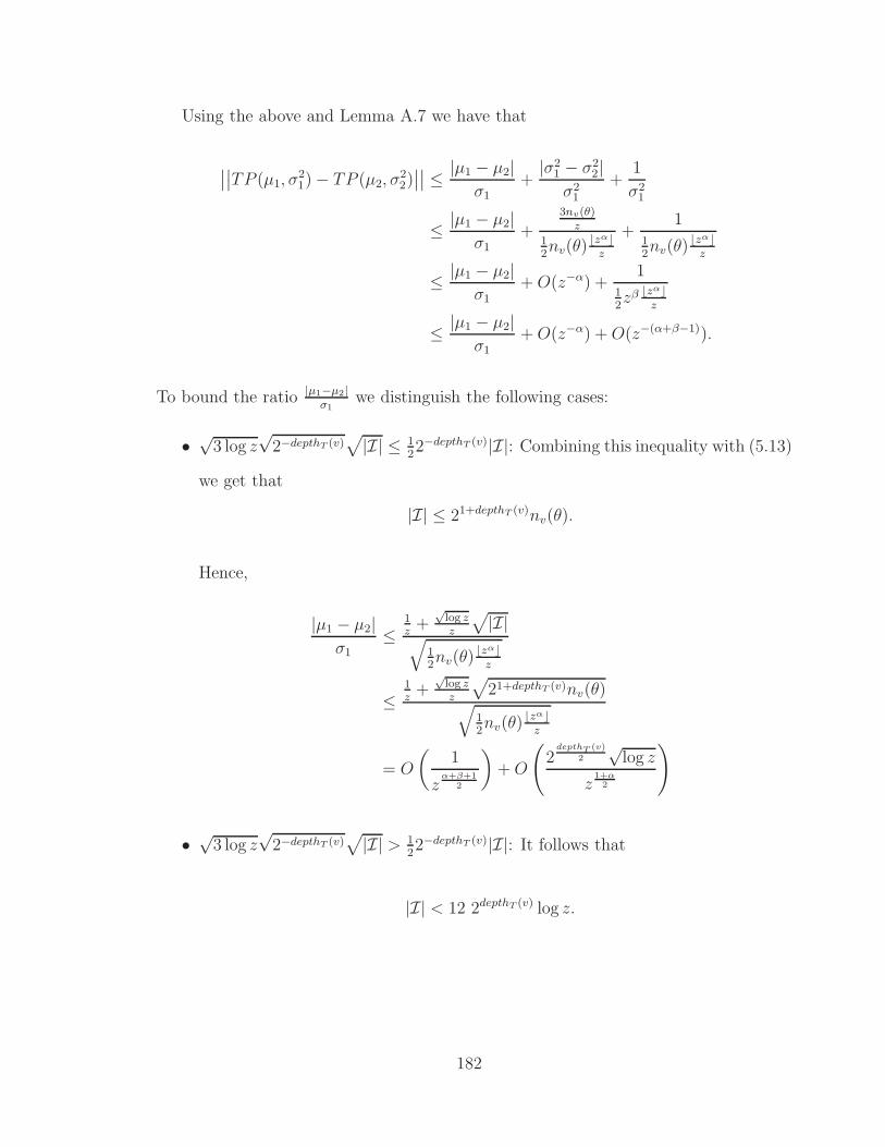
Using the above and Lemma A.7 we have that
∣∣∣∣TP (µ1, σ21) − TP (µ2, σ
22)∣∣∣∣ ≤ |µ1 − µ2|
σ1+
|σ21 − σ2
2|σ2
1
+1
σ21
≤ |µ1 − µ2|σ1
+3nv(θ)
z
12nv(θ) ⌊z
α⌋z
+1
12nv(θ) ⌊z
α⌋z
≤ |µ1 − µ2|σ1
+ O(z−α) +1
12zβ ⌊zα⌋
z
≤ |µ1 − µ2|σ1
+ O(z−α) + O(z−(α+β−1)).
To bound the ratio |µ1−µ2|σ1
we distinguish the following cases:
• √3 log z
√2−depthT (v)
√|I| ≤ 1
22−depthT (v)|I|: Combining this inequality with (5.13)
we get that
|I| ≤ 21+depthT (v)nv(θ).
Hence,
|µ1 − µ2|σ1
≤1z
+√
log zz
√|I|√
12nv(θ) ⌊z
α⌋z
≤1z
+√
log zz
√21+depthT (v)nv(θ)√
12nv(θ) ⌊z
α⌋z
= O
(1
zα+β+1
2
)+ O
(2
depthT (v)
2
√log z
z1+α
2
)
• √3 log z
√2−depthT (v)
√|I| > 1
22−depthT (v)|I|: It follows that
|I| < 12 2depthT (v) log z.
182
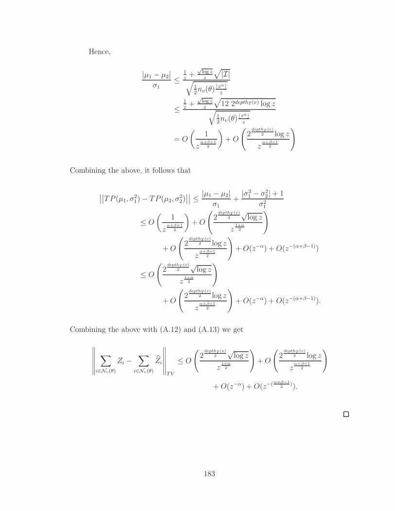
Hence,
|µ1 − µ2|σ1
≤1z
+√
log zz
√|I|√
12nv(θ) ⌊z
α⌋z
≤1z
+√
log zz
√12 2depthT (v) log z√
12nv(θ) ⌊z
α⌋z
= O
(1
zα+β+1
2
)+ O
(2
depthT (v)
2 log z
zα+β+1
2
)
Combining the above, it follows that
∣∣∣∣TP (µ1, σ21) − TP (µ2, σ
22)∣∣∣∣ ≤ |µ1 − µ2|
σ1+
|σ21 − σ2
2 | + 1
σ21
≤ O
(1
zα+β+1
2
)+ O
(2
depthT (v)
2
√log z
z1+α
2
)
+ O
(2
depthT (v)
2 log z
zα+β+1
2
)+ O(z−α) + O(z−(α+β−1))
≤ O
(2
depthT (v)
2
√log z
z1+α
2
)
+ O
(2
depthT (v)
2 log z
zα+β+1
2
)+ O(z−α) + O(z−(α+β−1)).
Combining the above with (A.12) and (A.13) we get
∥∥∥∥∥∥
∑
i∈Nv(θ)
Zi −∑
i∈Nv(θ)
Zi
∥∥∥∥∥∥TV
≤ O
(2
depthT (v)
2
√log z
z1+α
2
)+ O
(2
depthT (v)
2 log z
zα+β+1
2
)
+ O(z−α) + O(z−(α+β−12
)).
183
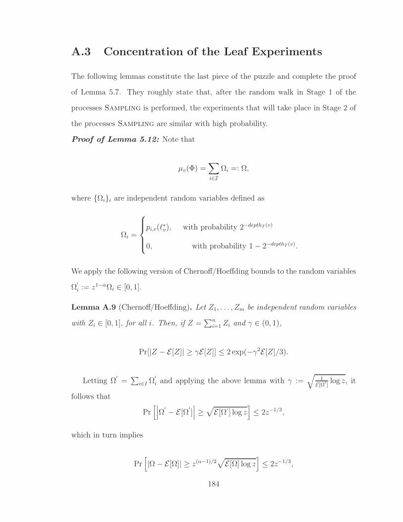
A.3 Concentration of the Leaf Experiments
The following lemmas constitute the last piece of the puzzle and complete the proof
of Lemma 5.7. They roughly state that, after the random walk in Stage 1 of the
processes Sampling is performed, the experiments that will take place in Stage 2 of
the processes Sampling are similar with high probability.
Proof of Lemma 5.12: Note that
µv(Φ) =∑
i∈IΩi =: Ω,
where Ωii are independent random variables defined as
Ωi =
pi,v(ℓ∗v), with probability 2−depthT (v)
0, with probability 1 − 2−depthT (v).
We apply the following version of Chernoff/Hoeffding bounds to the random variables
Ω′
i := z1−αΩi ∈ [0, 1].
Lemma A.9 (Chernoff/Hoeffding). Let Z1, . . . , Zm be independent random variables
with Zi ∈ [0, 1], for all i. Then, if Z =∑n
i=1 Zi and γ ∈ (0, 1),
Pr[|Z − E [Z]| ≥ γE [Z]] ≤ 2 exp(−γ2E [Z]/3).
Letting Ω′
=∑
i∈I Ω′
i and applying the above lemma with γ :=√
1E[Ω′ ]
log z, it
follows that
Pr[∣∣∣Ω′ − E [Ω
′]∣∣∣ ≥
√E [Ω′ ] log z
]≤ 2z−1/3,
which in turn implies
Pr[|Ω − E [Ω]| ≥ z(α−1)/2
√E [Ω] log z
]≤ 2z−1/3,
184
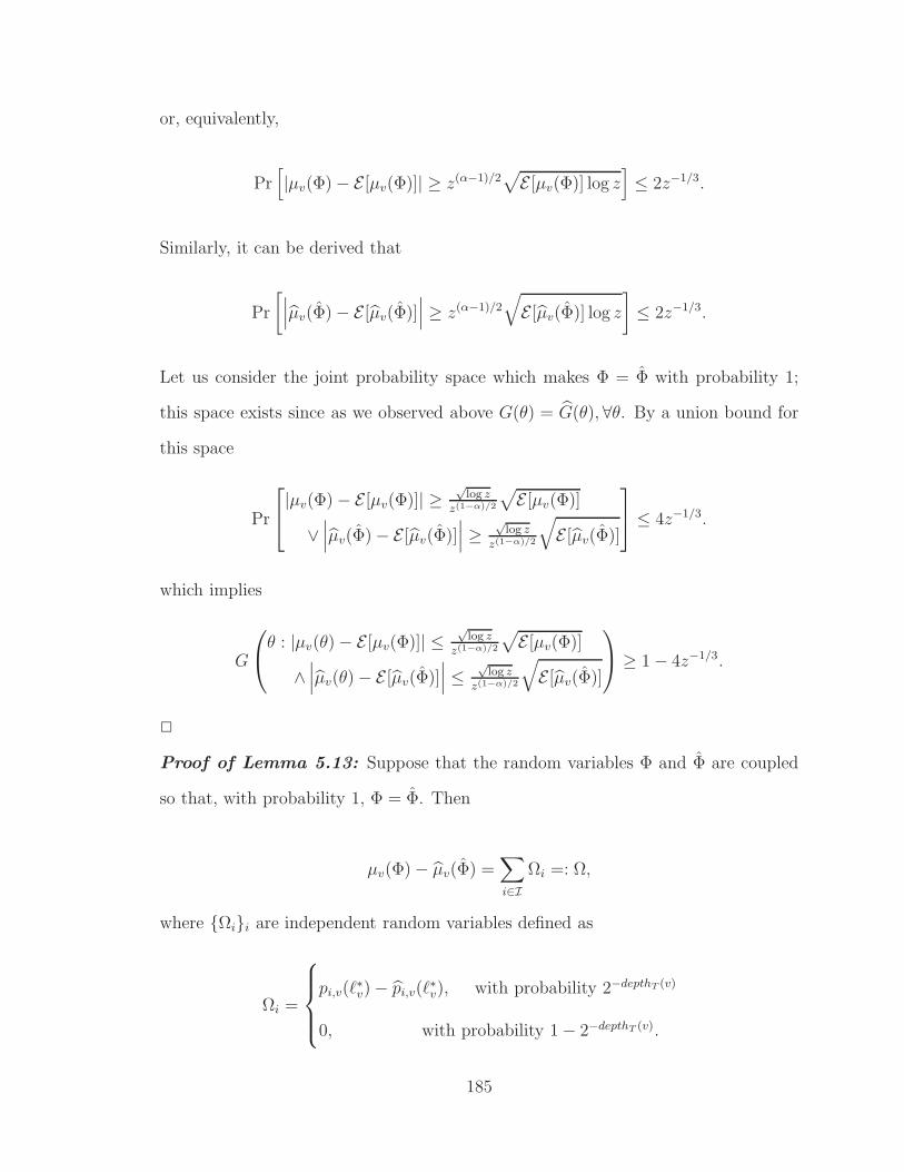
or, equivalently,
Pr[|µv(Φ) − E [µv(Φ)]| ≥ z(α−1)/2
√E [µv(Φ)] log z
]≤ 2z−1/3.
Similarly, it can be derived that
Pr
[∣∣∣µv(Φ) − E [µv(Φ)]∣∣∣ ≥ z(α−1)/2
√E [µv(Φ)] log z
]≤ 2z−1/3.
Let us consider the joint probability space which makes Φ = Φ with probability 1;
this space exists since as we observed above G(θ) = G(θ), ∀θ. By a union bound for
this space
Pr
|µv(Φ) − E [µv(Φ)]| ≥
√log z
z(1−α)/2
√E [µv(Φ)]
∨∣∣∣µv(Φ) − E [µv(Φ)]
∣∣∣ ≥√
log zz(1−α)/2
√E [µv(Φ)]
≤ 4z−1/3.
which implies
G
θ : |µv(θ) − E [µv(Φ)]| ≤√
log zz(1−α)/2
√E [µv(Φ)]
∧∣∣∣µv(θ) − E [µv(Φ)]
∣∣∣ ≤√
log zz(1−α)/2
√E [µv(Φ)]
≥ 1 − 4z−1/3.
2
Proof of Lemma 5.13: Suppose that the random variables Φ and Φ are coupled
so that, with probability 1, Φ = Φ. Then
µv(Φ) − µv(Φ) =∑
i∈IΩi =: Ω,
where Ωii are independent random variables defined as
Ωi =
pi,v(ℓ∗v) − pi,v(ℓ∗v), with probability 2−depthT (v)
0, with probability 1 − 2−depthT (v).
185
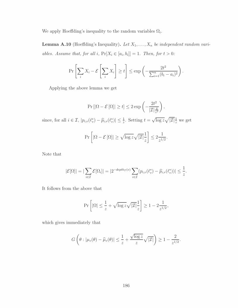
We apply Hoeffding’s inequality to the random variables Ωi.
Lemma A.10 (Hoeffding’s Inequality). Let X1, . . . , Xn be independent random vari-
ables. Assume that, for all i, Pr[Xi ∈ [ai, bi]] = 1. Then, for t > 0:
Pr
[∑
i
Xi − E[∑
i
Xi
]≥ t
]≤ exp
(− 2t2∑n
i=1(bi − ai)2
).
Applying the above lemma we get
Pr [|Ω − E [Ω]| ≥ t] ≤ 2 exp
(− 2t2
|I| 4z2
),
since, for all i ∈ I, |pi,v(ℓ∗v) − pi,v(ℓ∗v)| ≤ 1z. Setting t =
√log z
√|I|1
zwe get
Pr
[|Ω − E [Ω]| ≥
√log z
√|I|1
z
]≤ 2
1
z1/2.
Note that
|E [Ω]| = |∑
i∈IE [Ωi]| = |2−depthT (v)
∑
i∈I(pi,v(ℓ∗v) − pi,v(ℓ∗v))| ≤ 1
z.
It follows from the above that
Pr
[|Ω| ≤ 1
z+√
log z√
|I|1z
]≥ 1 − 2
1
z1/2,
which gives immediately that
G
(θ : |µv(θ) − µv(θ)| ≤ 1
z+
√log z
z
√|I|)
≥ 1 − 2
z1/2.
186
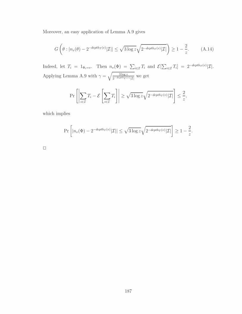
Moreover, an easy application of Lemma A.9 gives
G
(θ : |nv(θ) − 2−depthT (v)|I|| ≤
√3 log z
√2−depthT (v)|I|
)≥ 1 − 2
z. (A.14)
Indeed, let Ti = 1Φi=v. Then nv(Φ) =∑
i∈I Ti and E [∑
i∈I Ti] = 2−depthT (v)|I|.
Applying Lemma A.9 with γ =√
3 log z
2−depthT (v)|I| we get
Pr
[∣∣∣∣∣∑
i∈ITi − E
[∑
i∈ITi
]∣∣∣∣∣ ≥√
3 log z√
2−depthT (v)|I|]≤ 2
z,
which implies
Pr
[|nv(Φ) − 2−depthT (v)|I|| ≤
√3 log z
√2−depthT (v)|I|
]≥ 1 − 2
z.
2
187


![Computing Approximate Pure Nash Equilibria in Shapley ... · arXiv:1710.01634v2 [cs.GT] 27 Nov 2017 Computing Approximate Pure Nash Equilibria in Shapley Value Weighted Congestion](https://img.dokumen.tips/doc/110x75/5e6f2eb75ba3ca7ed40a34d7/computing-approximate-pure-nash-equilibria-in-shapley-arxiv171001634v2-csgt.jpg)