Function minimizationdesy.de/~blobel/blobel_minimize.pdf · 2007-03-22 · Function minimization Volker Blobel – University of Hamburg March 2005 1. Optimization 2. One-dimensional

Function minimization

Volker Blobel – University of HamburgMarch 2005

1. Optimization

2. One-dimensional minimization

3. Search methods

4. Unconstrained minimization

5. Derivative calculation

6. Trust-region methods

Keys during display: enter = next page; → = next page; ← = previous page; home = first page; end = last page (index, clickable); C-← = back; C-N = goto

page; C-L = full screen (or back); C-+ = zoom in; C-− = zoom out; C-0 = fit in window; C-M = zoom to; C-F = find; C-P = print; C-Q = exit.

Optimization in Physics data analysis

Objective function F (x) is

• (negative log of a) Likelihood function in the Maximum Likelihood method, or

• sum of squares in a (nonlinear) Least Squares problem

Constraints ci(x) are

• equality contraints, expressing relations between parameters, and

• inequality constraints are limits of certain parameters, defining a restricted range of parametervalues (e.g. m2

ν ≥ 0).

In mathematical terms:

minimize F (x) x ∈ Rn

subject to ci(x) = 0, i =1, 2, . . . m′

ci(x) ≥ 0, i =m′ + 1, . . .m

Sometimes there are two objective functions: F (x), requiring a good data description, and G(x),requiring e.g. smoothness:

minimize sum F (x) + τ ·G(x)

with weight parameter τ .

Volker Blobel – University of Hamburg Function minimization page 2

Aim of optimization

• Find the global minimum of the objective function F (x),

• within the allowed range of parameter values,

• in a short time even for a large number of parameters and a complicated objective function,

• even is there are local minima.

Most methods will converge to the next minimum, which may be the global minimum or a localminimum (corresponding to rapid cooling), going immediately downhill as far as possible.

Search for the global minimum requires a special effort.


A special case: combinatorical minimization

The travelling salesman problem:

Find the shortest cyclical itenary for a travelling salesman who must visit each of N citiesin turn.

Space over which the function is defined is a discrete, but very large, configuration space (e.g. set ofpossible orders of cities), with a number of elements in the configuration space which is factorial large(remember: 69! ≈ 10100). The concept of a “direction” may have no meaning.

Objective function is e.g. the total path length.


. . . contnd.

Desired global extremum may be hidden among many, poorer, local extrema.

Nature is, for slowly cooled systems, able to find the minimum energy state of a crystalthat is completely ordered over a large distance.

The method: Simulated annealing, in analogy with the way metals cool and anneal, with slow cooling,using Boltzmanns probability distribution

Prob(E) ∼ exp (−E/kBT )

for a systen in equilibrium.

Even at low T there is a chance for a higher energy state, with a corresponding chance to get out of alocal minimum.


The Metropolis algorithm: the elements

• A description of possible system configurations.

• A generator of random changes in the configuration (called “option”).

• An objective function E (analog of energy) whose minimizatiuon is the goal of the procedure.

• A control parameter T (analog of temperature) and an annealing schedule (for cooling down).

A random option will change the configuration from energy E1 to energy E2. This option is acceptedwith probability

p = exp

[−(E2 − E1)

kbT

]

Note: if E2 < E1 the option is always accepted.

Example: the “effective” solution of the travelling salesman problem


One-dimensional minimization

Search for minimum of function f(x) of (scalar) argument x.

Important application in multidimensional minimization: robust minimization along a line

f(z) = F (x + z ·∆x) Line search

Aim: robust, efficient and as fast as possible, because each function evaluation my require a large cputime.

Standard method: iterations, starting from x0, with expression Φ(x):

xk+1 = Φ(xk) for k = 0, 1, 2, . . .

with convergence to fixed point x∗ with x∗ = Φ(x∗)


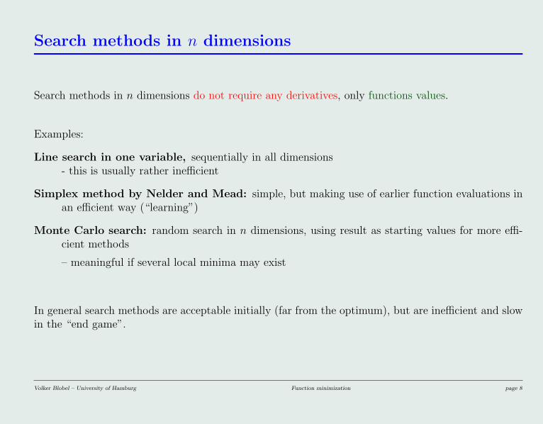
Search methods in n dimensions

Search methods in n dimensions do not require any derivatives, only functions values.

Examples:

Line search in one variable, sequentially in all dimensions- this is usually rather inefficient

Simplex method by Nelder and Mead: simple, but making use of earlier function evaluations inan efficient way (“learning”)

Monte Carlo search: random search in n dimensions, using result as starting values for more effi-cient methods

– meaningful if several local minima may exist

In general search methods are acceptable initially (far from the optimum), but are inefficient and slowin the “end game”.


Simplex method in n dimensions

A simplex is formed by n + 1 points in n-dimensional space (n = 2 triangle)

x1, x2, . . .xn, xn+1

sorted such that function values Fj = F (xj) are in the order

F1 ≤ F2 ≤ . . . Fn ≤ Fn+1

In addition: mean of best n points =

center of gravity c =1

n

n∑j=1

xj

Method: sequence of cycles with new point in each cycle, replacing worst point xn+1, with new(updated) simplex in each cycle.

At the start of each cycle new test point xr, obtained by reflexion of worst point at the center ofgravity:

xr = c + α · (c− xn+1)


A cycle in the Nelder and Mead method

Depending on value F (xr):

[F1 ≤ Fr ≤ Fn ]: Test point xr is middle point and is added, the previous worst point is removed.

[Fr ≤ F1 ]: Test point xr is best point, search direction seems to be effective. A new point xs =c + β · (xr − c) (with β > 1) is determined and the function value is Fs evaluated. For Fs < Fr

the extra step is successful, xn+1 is replaced by xs otherwise by xr.

[Fr > Fn ]: the simplex is too big and has to be reduced in size. For Fr < Fn+1 the test pointxr replaces the words point xn+1. A new test point xs is defined by xs = c − γ(c − xn+1)(contraction) with 0 < γ < 1. If this point xs with Fs = F (xs) < Fn+1 is an improvement, thenxn+1 is replaced by this point xs. Otherwise a new simplex in defined by replacing all pointsexcept x1 by xj = x1 + δ(xj −x1) for j = 2, . . . n + 1 with 0 < δ < 1, which requires n functionevaluations.

Typical values are α = 1, β = 2, γ = 0.5 und δ = 0.5.


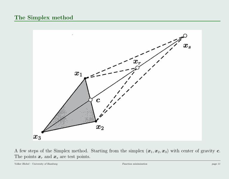
The Simplex method

A few steps of the Simplex method. Starting from the simplex (x1, x2, x3) with center of gravity c.The points xr and xs are test points.


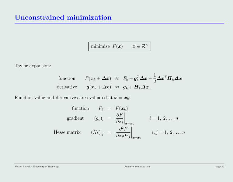
Unconstrained minimization

minimize F (x) x ∈ Rn

Taylor expansion:

function F (xk + ∆x) ≈ Fk + gTk ∆x +

1

2∆xT Hk∆x

derivative g(xk + ∆x) ≈ gk + Hk∆x ,

Function value and derivatives are evaluated at x = xk:

function Fk = F (xk)

gradient (gk)i =∂F

∂xi

∣∣∣∣x=xk

i = 1, 2, . . . n

Hesse matrix (Hk)ij =∂2F

∂xi∂xj

∣∣∣∣x=xk

i, j = 1, 2, . . . n


Covariance matrix for statistical objective functions

Note: if the objective function is

• a sum of squares of deviations, defined according to the Method of Least Squares, or

• a negative log. Likelihood function, defined according to the Maximum Likelihood Method,

then the inverse Hessian H at the minimum is a good estimate of the covariance matrix of theparameters x:

V x ≈ H−1


The Newton step

Step ∆xN determined from gk + Hk∆x = 0:

∆xN = −H−1k gk .

For a quadratic function F (x) the Newton step is, in length and direction, a step to the minimumof the function.

Sometimes large angle (≈ 90◦) between Newton direction ∆xN and gk (the direction of steepestdescent).

Calculation of the distance ∆F to the minimum (called EDM in Minuit):

d = −gTk ·∆xN = gT

k H−1k gk = ∆xT

NHk∆xN > 0

if Hessian positive-definite. For a quadratic function the distance to the minimum is d/2.


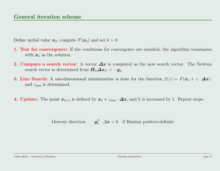
General iteration scheme

Define initial value x0, compute F (x0) and set k = 0

1. Test for convergence: If the conditions for convergence are satisfied, the algorithm terminateswith xk as the solution.

2. Compute a search vector: A vector ∆x is computed as the new search vector. The Newtonsearch vector is determined from Hk∆xN = −gk.

3. Line Search: A one-dimensional minimization is done for the function f(z) = F (xk + z · ∆x).and zmin is determined.

4. Update: The point xk+1 is defined by xk + zmin ·∆x, and k is increased by 1. Repeat steps.

Descent direction gTk ·∆x < 0 if Hessian positive-definite


Method of steepest descent

The search vector ∆x is equal to the negative gradienten

∆xSD = −gk

• Step seems to be natural choice;

• only gradient required (no Hesse matrix) – good;

• no step size defined (in contrast to the Newton step) – bad;

• rate of convergence only linear:

F (xk+1)− F (x∗)

F (xk)− F (x∗)= c ≈

(λmax − λmin

λmax + λmin

)2

=

(κ− 1

κ + 1

)2

,

(λmax and λmin are largest and smallest eigenvalue and κ condition number of Hesse matrix H .For a large value of κ c close to one and slow convergence – very bad.

Optimal step including size, if Hesse matrix known:

∆xSD = −(

gTk gk

gTk Hkgk

)gk .


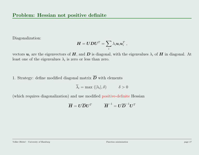
Problem: Hessian not positive definite

Diagonalization:

H = UDUT =∑

i

λiuiuTi ,

vectors ui are the eigenvectors of H , and D is diagonal, with the eigenvalues λi of H in diagonal. Atleast one of the eigenvalues λi is zero or less than zero.

1. Strategy: define modified diagonal matrix D with elements

λi = max (|λi|, δ) δ > 0

(which requires diagonalization) and use modified positive-definite Hessian

H = UDUT H−1

= UD−1

UT


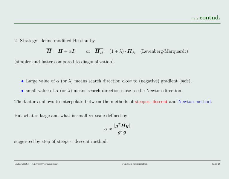
. . . contnd.

2. Strategy: define modified Hessian by

H = H + αIn or Hjj = (1 + λ) ·Hjj (Levenberg-Marquardt)

(simpler and faster compared to diagonalization).

• Large value of α (or λ) means search direction close to (negative) gradient (safe),

• small value of α (or λ) means search direction close to the Newton direction.

The factor α allows to interpolate between the methods of steepest descent and Newton method.

But what is large and what is small α: scale defined by

α ≈ |gT Hg|gT g

suggested by step of steepest descent method.


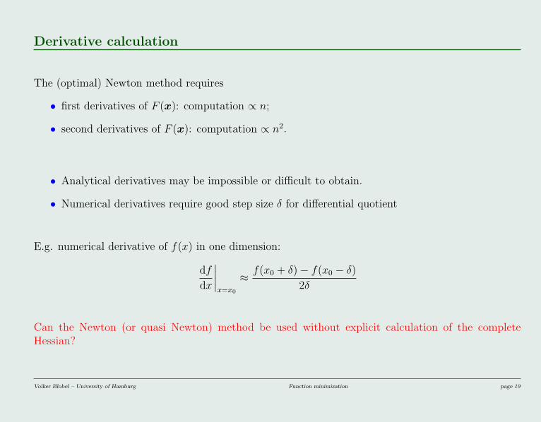
Derivative calculation

The (optimal) Newton method requires

• first derivatives of F (x): computation ∝ n;

• second derivatives of F (x): computation ∝ n2.

• Analytical derivatives may be impossible or difficult to obtain.

• Numerical derivatives require good step size δ for differential quotient

E.g. numerical derivative of f(x) in one dimension:

df

dx

∣∣∣∣x=x0

≈ f(x0 + δ)− f(x0 − δ)

2δ

Can the Newton (or quasi Newton) method be used without explicit calculation of the completeHessian?


Variable metrik method

Calculation of Hessian (with n(n+1)/2 different elements) from sequence of first derivatives (gradients):by update of estimate Hk from change of gradient.

• Step ∆x is calculated from Hk ∆x = −gk

• After a line search with minimum at zmin new value is xk+1 = xk + zmin ∆x,with gradient gk+1.

• Update matrix: U k is added to Hk to get new estimate of Hessian:

Hk+1 = Hk + U k

Hk+1δ = γ δ = xk+1 − xk γ = gk+1 − gk

(with γT δ > 0)

Note: an accurate line search is essential for the success.


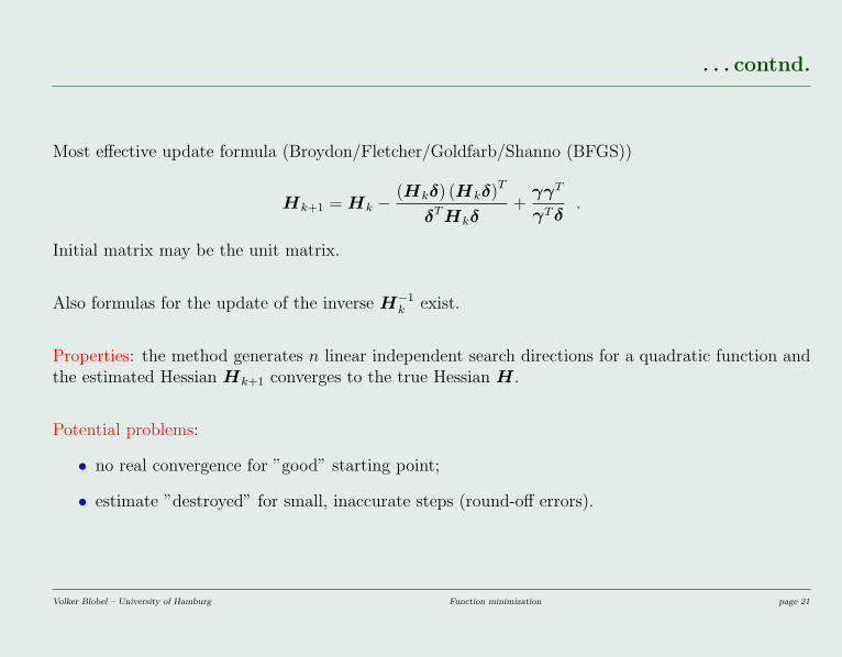
. . . contnd.

Most effective update formula (Broydon/Fletcher/Goldfarb/Shanno (BFGS))

Hk+1 = Hk −(Hkδ) (Hkδ)T

δT Hkδ+

γγT

γT δ.

Initial matrix may be the unit matrix.

Also formulas for the update of the inverse H−1k exist.

Properties: the method generates n linear independent search directions for a quadratic function andthe estimated Hessian Hk+1 converges to the true Hessian H .

Potential problems:

• no real convergence for ”good” starting point;

• estimate ”destroyed” for small, inaccurate steps (round-off errors).


Example: Minuit from Cern

Several options can be selected:

Option MIGRAD: minimizes the objective function, calculates first derivatives numerically anduses the BFGS update formula for the Hessian – fast (if it works)

Option HESSE: calculates the Hesse matrix numerically – recommended after minimization

Option MINIMIZE: minimization by MIGRAD and HESSE calculation with checks.

Restricted range of parameters possible: by transformation from a finite range (of external variables)to −∞ . . . +∞ (of internal variables) using trigonometrical functions.

• allows to use minimization algorithm without range restriction;

• good (quadratic) function is transformed perhaps to a difficult function;

• range specification may be bad, e.g [0, 108] for optimum at 1.


Derivative calculation

Efficient minimization must take first and second order derivatives into account, which allows to applyNewton’s principle.

Numerical methods for derivative calculation of F (x) by finite differences

• require a good step length – not to small (roundoff errors) and not too large (influence of higherderivatives);

• require very many (time consuming) function evaluations.

Variable metrik methods allow to avoid the calculation of second derivatives of F (x), but still needthe first derivative.Are there other possibilities?

• the Gauss-Newton method, which reduces the derivative calculation; the Hessian can be calcu-lated (estimated) without having to compute second derivatives;

• automatic derivative calculation.


Least squares curve fit

Assume a least squares fit of a curve f(xi, a) with parameters a to Gaussian distributed data yi withweight wi = 1/σ2

i :yi∼= f(xi, a)

Negative Log of the likelihood function is equal to the sum of squares:

F (a) =∑

i

wi (f(xi, a)− yi)2

Derivatives of F (a) are determined by derivatives of f(xi, a):

∂F

∂aj

=∑

i

wi∂f

∂aj

(f(xi, a)− yi)

∂2F

∂aj∂ak

=∑

i

wi∂f

∂aj

∂f

∂ak

+∑

i

wi∂2f

∂aj∂ak

(f(xi, a)− yi)

Usually the contributions from second derivatives of f(xi, a) are small and can be neglected; theapproximate Hessian from first derivatives of f(xi, a) has positive diagonal elements and is expectedto be positive-definite. The use of the approximate Hessian is called Gauss-Newton method.


Poisson contribution to objective function

Assume a maximum-likelihood fit of a function f(xi, a) with parameters a to Poisson-distributed datayi:

yi∼= f(xi, a)

Negative Log of the likelihood function:

F (a) =∑

i

f(xi, a)− yi ln f(xi, a)

or better F (a) =∑

i

(f(xi, a)− yi) + yi lnyi

f(xi, a)

Derivatives of F (a) are determined by derivatives of f(xi, a):

∂F

∂aj

=∑

i

yi

∂f∂aj

f(xi, a)− ∂f

∂aj

∂2F

∂aj∂ak

=∑

i

yi

∂f∂aj

∂f∂ak

− ∂2f∂aj∂ak

f(xi, a)

f 2(xi, a)−

∑i

∂2f

∂aj∂ak

Usually the contributions from second derivatives of f(xi, a) are small and and can be neglected; theapproximate Hessian from first derivatives of f(xi, a) has positive diagonal elements and is expectedto be positive-definite. The use of the approximate Hessian is called Gauss-Newton method.


Automatic differentiation

Can automatic differentiation be used?

GNU libmatheval is a library comprising several procedures that makes it possible to create in-memorytree representation of mathematical functions over single or multiple variables and later use this rep-resentation to evaluate function for specified variable values, to create corresponding tree for functionderivative over specified variable or to get back textual representation of in-memory tree.

Calculated derivative is in mathematical sense correct no matters of fact that derivation variableappears or not in function represented by evaluator.

Supported elementary functions are: exponential (exp), logarithmic (log), square root (sqrt), sine (sin), cosine (cos),tangent (tan), cotangent (cot), secant (sec), cosecant (csc), inverse sine (asin), inverse cosine (acos), inverse tangent(atan), inverse cotangent (acot), inverse secant (asec), inverse cosecant (acsc), hyperbolic sine (sinh), cosine (cosh),hyperbolic tangent (tanh), hyperbolic cotangent (coth), hyperbolic secant (sech), hyperbolic cosecant (csch), hyperbolicinverse sine (asinh), hyperbolic inverse cosine (acosh), hyperbolic inverse tangent (atanh), hyperbolic inverse cotangent(acoth), hyperbolic inverse secant (asech), hyperbolic inverse cosecant (acsch), absolute value (abs), Heaviside stepfunction (step) with value 1 defined for x = 0 and Dirac delta function with infinity (delta) and not-a-number (nandelta)values defined for x = 0.


Trust-region methods

If the derivatives of F (x) are available the quadratic model

F̃ (xk + d) = Fk + gTk d +

1

2dT Hkd

can be written at the point xk with the gradient gk ≡ ∇F and the Hessian Hk ≡ ∇2F (matrix ofsecond derivatives). From the approximation the step d is calculated from

gk + Hkd = 0

which isd = −H−1

k gk .

In the trust-region method the model is restricted depending on a parameter ∆, which forces thenext iterate into a sphere centered at xk and of radius ∆, which defines the trust region, where themodel is assumed to be acceptable. The vector d is determined by solving

minimize F̃ (xk + d), |d| ≤ ∆ ,

a constrained quadratic minimization problem. The equation can be solved efficiently even if theHessian is not positive-definite.


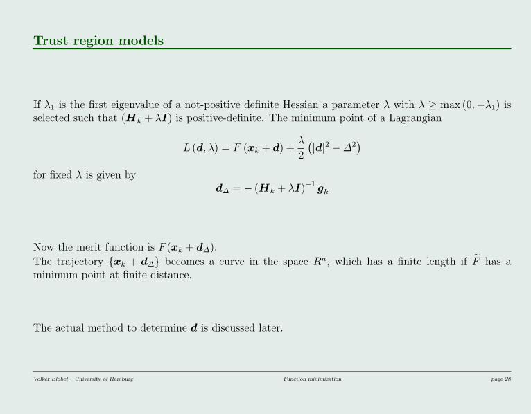
Trust region models

If λ1 is the first eigenvalue of a not-positive definite Hessian a parameter λ with λ ≥ max (0,−λ1) isselected such that (Hk + λI) is positive-definite. The minimum point of a Lagrangian

L (d, λ) = F (xk + d) +λ

2

(|d|2 −∆2

)for fixed λ is given by

d∆ = − (Hk + λI)−1 gk

Now the merit function is F (xk + d∆).

The trajectory {xk + d∆} becomes a curve in the space Rn, which has a finite length if F̃ has aminimum point at finite distance.

The actual method to determine d is discussed later.


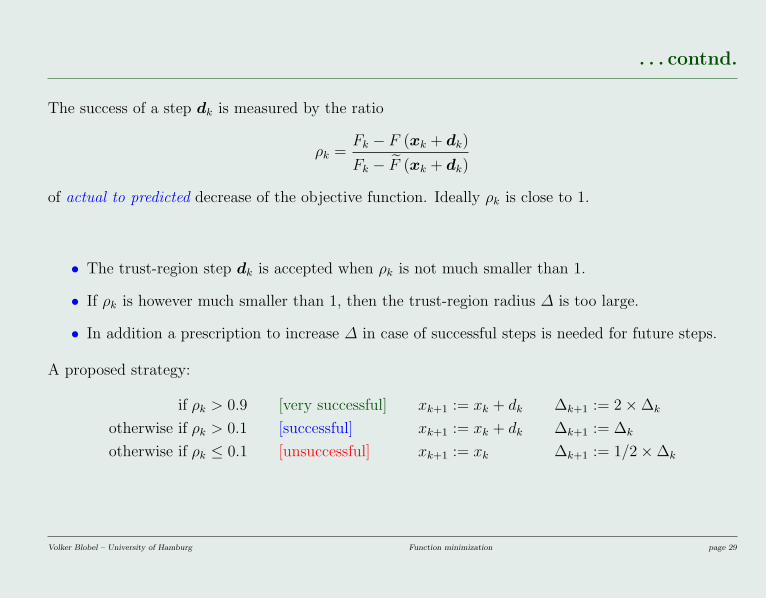
. . . contnd.

The success of a step dk is measured by the ratio

ρk =Fk − F (xk + dk)

Fk − F̃ (xk + dk)

of actual to predicted decrease of the objective function. Ideally ρk is close to 1.

• The trust-region step dk is accepted when ρk is not much smaller than 1.

• If ρk is however much smaller than 1, then the trust-region radius ∆ is too large.

• In addition a prescription to increase ∆ in case of successful steps is needed for future steps.

A proposed strategy:

if ρk > 0.9 [very successful] xk+1 := xk + dk ∆k+1 := 2×∆k

otherwise if ρk > 0.1 [successful] xk+1 := xk + dk ∆k+1 := ∆k

otherwise if ρk ≤ 0.1 [unsuccessful] xk+1 := xk ∆k+1 := 1/2×∆k


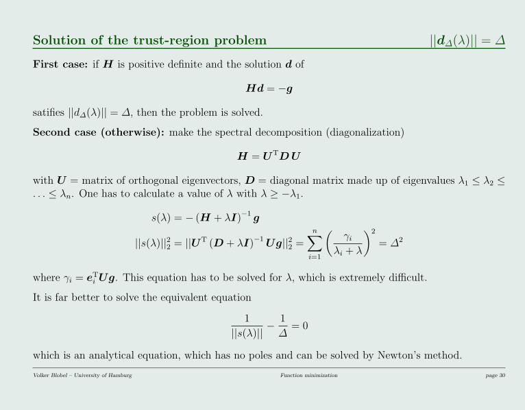
Solution of the trust-region problem ||d∆(λ)|| = ∆

First case: if H is positive definite and the solution d of

Hd = −g

satifies ||d∆(λ)|| = ∆, then the problem is solved.

Second case (otherwise): make the spectral decomposition (diagonalization)

H = UTD U

with U = matrix of orthogonal eigenvectors, D = diagonal matrix made up of eigenvalues λ1 ≤ λ2 ≤. . . ≤ λn. One has to calculate a value of λ with λ ≥ −λ1.

s(λ) = − (H + λI)−1 g

||s(λ)||22 = ||UT (D + λI)−1 Ug||22 =n∑

i=1

(γi

λi + λ

)2

= ∆2

where γi = eTi Ug. This equation has to be solved for λ, which is extremely difficult.

It is far better to solve the equivalent equation

1

||s(λ)||− 1

∆= 0

which is an analytical equation, which has no poles and can be solved by Newton’s method.


Properties of trust-region methods

Opinions about trust-region methods:

“The trust-region method is actually extremely important and might supersede line-searches, sooneror later.”

“Trust-region methods are not superior to methods with step-length strategy; at least the number ofiterations is higher. . . . they are not more robust.”

Parameters can be of very different order of magnitude and precision. Preconditioning with appropriatescaling of the parameters may be essential for the trust-region method.

Linesearch-methods are naturally optimistic,while trust-region methods appear to be naturally pessimistic. Trust-region methods are expected tobe more robust, with convergence (perhaps slower) even in difficult cases.


Function minimizationOptimization in Physics data analysis . . . . . . . . . . . . 2Aim of optimization . . . . . . . . . . . . . . . . . . . . . . 3A special case: combinatorical minimization . . . . . . . . . 4The Metropolis algorithm: the elements . . . . . . . . . . . 6

One-dimensional minimization 7

Search methods in n dimensions 8Simplex method in n dimensions . . . . . . . . . . . . . . . 9A cycle in the Nelder and Mead method . . . . . . . . . . . 10The Simplex method . . . . . . . . . . . . . . . . . . . . . . 11

Unconstrained minimization 12Covariance matrix for statistical objective functions . . . . 13The Newton step . . . . . . . . . . . . . . . . . . . . . . . . 14General iteration scheme . . . . . . . . . . . . . . . . . . . . 15Method of steepest descent . . . . . . . . . . . . . . . . . . 16Problem: Hessian not positive definite . . . . . . . . . . . . 17Derivative calculation . . . . . . . . . . . . . . . . . . . . . 19Variable metrik method . . . . . . . . . . . . . . . . . . . . 20Example: Minuit from Cern . . . . . . . . . . . . . . . . . 22

Derivative calculation 23Least squares curve fit . . . . . . . . . . . . . . . . . . . . . 24Poisson contribution to objective function . . . . . . . . . . 25Automatic differentiation . . . . . . . . . . . . . . . . . . . 26

Trust-region methods 27Trust region models . . . . . . . . . . . . . . . . . . . . . . 28Solution of the trust-region problem . . . . . . . . . . . . . 30Properties of trust-region methods . . . . . . . . . . . . . . 31

Documents

Function minimizationdesy.de/~blobel/blobel_minimize.pdf · 2007-03-22 · Function minimization Volker Blobel – University of Hamburg March 2005 1. Optimization 2. One-dimensional