Embed Size (px)
Citation preview

FROM QUALITATIVE TO QUANTITATIVEEVALUATION METHODS IN
MULTI-CRITERIA DECISION MODELS
Mag. Biljana Mileva Boshkoska

Doctoral DissertationJožef Stefan International Postgraduate SchoolLjubljana, Slovenia, November 2013
Evaluation Board:Prof. Dr. Sašo Džeroski, Chairman, Jožef Stefan Institute, Jamova 39, Ljubljana, SloveniaAsst. Prof. Dr. Martin Žnidaršic, Member, Jožef Stefan Institute, Jamova 39, Ljubljana, SloveniaProf. Dr. Vladislav Rajkovic, Member, University of Maribor, Kidriceva cesta 55a, Kranj, Slovenia

MEDNARODNA PODIPLOMSKA ŠOLA JOŽEFA STEFANAJOŽEF STEFAN INTERNATIONAL POSTGRADUATE SCHOOLLjubljana, Slovenia
SLOVENIA
LJUBLJANA
JOŽEF ST
EFA
N I
NT
ERNATIONAL POSTGR
AD
UA
TE
SCHOOL
2004
Mag. Biljana Mileva Boshkoska
FROM QUALITATIVE TOQUANTITATIVE EVALUATIONMETHODS IN MULTI-CRITERIADECISION MODELS
Doctoral Dissertation
OD KVALITATIVNIH DOKVANTITATIVNIH METODVREDNOTENJA VVECPARAMETRSKIHODLOCITVENIH MODELIH
Doktorska disertacija
Supervisor: Prof. Dr. Marko Bohanec
Ljubljana, Slovenia, November 2013


V
Index
Abstract IX
Povzetek XI
List of Abbreviations XII
1 Introduction 11.1 Aims and Hypothesis . . . . . . . . . . . . . . . . . . . . . . . . . . . . . . . . . . . . 21.2 Research Methodology and Specific Contributions . . . . . . . . . . . . . . . . . . . . 21.3 Organization of the Thesis . . . . . . . . . . . . . . . . . . . . . . . . . . . . . . . . . 3
2 Formal Description of the Problem 72.1 Problem Formulation . . . . . . . . . . . . . . . . . . . . . . . . . . . . . . . . . . . . 72.2 Structure of the Decision Model . . . . . . . . . . . . . . . . . . . . . . . . . . . . . . 102.3 Variability as a Measure for Ranking . . . . . . . . . . . . . . . . . . . . . . . . . . . . 102.4 Running Example . . . . . . . . . . . . . . . . . . . . . . . . . . . . . . . . . . . . . . 10
3 From Qualitative to Quantitative Multi-Criteria Models 133.1 Qualitative Decision Making Methods . . . . . . . . . . . . . . . . . . . . . . . . . . . 133.2 Qualitative Modeling with DEX . . . . . . . . . . . . . . . . . . . . . . . . . . . . . . 143.3 The Qualitative-Quantitative Method . . . . . . . . . . . . . . . . . . . . . . . . . . . . 16
4 Modifications of QQ with Impurity Functions, Polynomials and Optimization Functions 214.1 Impurity Functions for Weights Estimation in QQ . . . . . . . . . . . . . . . . . . . . . 21
4.1.1 Gini Index . . . . . . . . . . . . . . . . . . . . . . . . . . . . . . . . . . . . . 224.1.2 Chi Square χ2 . . . . . . . . . . . . . . . . . . . . . . . . . . . . . . . . . . . 244.1.3 Information Gain . . . . . . . . . . . . . . . . . . . . . . . . . . . . . . . . . . 254.1.4 Weights Calculation with Impurity Functions . . . . . . . . . . . . . . . . . . . 25
4.2 Polynomial Models for Regression . . . . . . . . . . . . . . . . . . . . . . . . . . . . . 264.2.1 CIPER . . . . . . . . . . . . . . . . . . . . . . . . . . . . . . . . . . . . . . . 264.2.2 New CIPER . . . . . . . . . . . . . . . . . . . . . . . . . . . . . . . . . . . . . 28
4.3 Reformulation of the Problem as Optimization Problem with Constraints . . . . . . . . . 314.4 Implementation of the QQ-Based Algorithms . . . . . . . . . . . . . . . . . . . . . . . 34
5 Copula Theory 355.1 Basic Concepts of the Probability Theory . . . . . . . . . . . . . . . . . . . . . . . . . 355.2 Quantile Regression . . . . . . . . . . . . . . . . . . . . . . . . . . . . . . . . . . . . . 375.3 Copula Functions . . . . . . . . . . . . . . . . . . . . . . . . . . . . . . . . . . . . . . 38
5.3.1 Archimedean Copulas and Connection to T-norms . . . . . . . . . . . . . . . . 40

VI INDEX
5.3.2 Estimation of the Parameter θ . . . . . . . . . . . . . . . . . . . . . . . . . . . 415.3.3 Interpretation of the Parameter θ . . . . . . . . . . . . . . . . . . . . . . . . . . 42
5.4 Higher-Dimensional Copulas . . . . . . . . . . . . . . . . . . . . . . . . . . . . . . . . 425.4.1 One-Parametric Archimedean Multi-Variate Copulas . . . . . . . . . . . . . . . 435.4.2 Specific Derivation for Multi-Variate Clayton Copula . . . . . . . . . . . . . . . 445.4.3 Fully Nested Archimedean Constructions . . . . . . . . . . . . . . . . . . . . . 445.4.4 Partially Nested Archimedean Constructions . . . . . . . . . . . . . . . . . . . 455.4.5 Conditions for FNAC and PNAC . . . . . . . . . . . . . . . . . . . . . . . . . . 46
5.5 Kernel Smoothing of Attribute’s Distributions in Hierarchical DEX Models . . . . . . . 47
6 Regression Using Nested Archimedean Copulas 496.1 Quantile Regression . . . . . . . . . . . . . . . . . . . . . . . . . . . . . . . . . . . . . 506.2 Regression with FNAC: Different Positions of Dependent Variable in the Input Level in
the FNAC . . . . . . . . . . . . . . . . . . . . . . . . . . . . . . . . . . . . . . . . . . 536.3 Regression with PNAC: Case of Four and Five Attributes and Generalization to n Attributes 546.4 Number of Possible FNAC and PNAC Structures . . . . . . . . . . . . . . . . . . . . . 566.5 Running Example for Regression Using FNAC . . . . . . . . . . . . . . . . . . . . . . 576.6 Copula-Based Option Ranking Algorithms . . . . . . . . . . . . . . . . . . . . . . . . . 58
6.6.1 Regression Algorithms for FNAC and PNAC . . . . . . . . . . . . . . . . . . . 606.6.2 Implementation of the Copula-Based Algorithms . . . . . . . . . . . . . . . . . 63
6.7 Hierarchical Running Example for Usage of Copula-Based Option Ranking Algorithm . 63
7 Experimental Evaluation on Artificially Generated Data Sets 657.1 Datasets . . . . . . . . . . . . . . . . . . . . . . . . . . . . . . . . . . . . . . . . . . . 657.2 Evaluation Results of the Performed Experiments . . . . . . . . . . . . . . . . . . . . . 65
7.2.1 Results from Copula-Based Methods . . . . . . . . . . . . . . . . . . . . . . . 667.2.2 Results from Experiments Based on Constraint Optimization Approach . . . . . 707.2.3 Results from Experiments Based on CIPER and New CIPER . . . . . . . . . . . 707.2.4 Results Obtained with QQ when Modified with Impurity Functions . . . . . . . 717.2.5 Time Execution of Methods . . . . . . . . . . . . . . . . . . . . . . . . . . . . 72
7.3 Summary . . . . . . . . . . . . . . . . . . . . . . . . . . . . . . . . . . . . . . . . . . 73
8 Illustrative Examples 758.1 FNAC Solves the Breaching Monotonicity . . . . . . . . . . . . . . . . . . . . . . . . . 758.2 PNAC Solves the Breaching Monotonicity . . . . . . . . . . . . . . . . . . . . . . . . . 768.3 Evaluation of Symmetric Decision Tables . . . . . . . . . . . . . . . . . . . . . . . . . 78
9 Applications of Copula-Based Method for Option Ranking 819.1 Assessment of Electrically Commutated Motors . . . . . . . . . . . . . . . . . . . . . . 81
9.1.1 Feature Selection and Organization in DEX Structure . . . . . . . . . . . . . . . 829.1.2 Implementation Within the Quality Assessment System . . . . . . . . . . . . . . 849.1.3 Qualitative to Quantitative Value Mapping . . . . . . . . . . . . . . . . . . . . . 859.1.4 Integration of Feature Values and Expert’s Preferences . . . . . . . . . . . . . . 869.1.5 Constructing the Copula-Based Regression Functions . . . . . . . . . . . . . . . 879.1.6 The Final Evaluation of EC Motors and Two Characteristic Examples . . . . . . 899.1.7 Discussion . . . . . . . . . . . . . . . . . . . . . . . . . . . . . . . . . . . . . 91
9.2 Assessment of Workflows . . . . . . . . . . . . . . . . . . . . . . . . . . . . . . . . . . 929.2.1 Data-Mining Workflow Assessment . . . . . . . . . . . . . . . . . . . . . . . . 929.2.2 Models for Ranking DW Options . . . . . . . . . . . . . . . . . . . . . . . . . 93

INDEX VII
9.2.3 Experimental Evaluation . . . . . . . . . . . . . . . . . . . . . . . . . . . . . . 94
10 Conclusions 9910.1 Contributions of the thesis . . . . . . . . . . . . . . . . . . . . . . . . . . . . . . . . . 9910.2 Future Work . . . . . . . . . . . . . . . . . . . . . . . . . . . . . . . . . . . . . . . . . 100
11 Acknowledgements 103
12 References 105
Publications related to the dissertation 111
Index of Figures 113
Index of Tables 115
Index of Algorithms 117
Appendix 119A Distribution of results with different tables . . . . . . . . . . . . . . . . . . . . . . . . . 119B Illustrative examples: rankings with different methods . . . . . . . . . . . . . . . . . . . 121
B.1 Appendix to Section 8.1 . . . . . . . . . . . . . . . . . . . . . . . . . . . . . . 121B.2 Appendix to Section 8.2 . . . . . . . . . . . . . . . . . . . . . . . . . . . . . . 122B.3 Appendix to Section 8.3 . . . . . . . . . . . . . . . . . . . . . . . . . . . . . . 124
C Specific derivations for multi-variate Frank and Gumbel copulas . . . . . . . . . . . . . 126C.1 Specific derivation for multi-variate Frank copula . . . . . . . . . . . . . . . . . 126C.2 Specific derivation for multi-variate Gumbel copula . . . . . . . . . . . . . . . . 126
D Biography . . . . . . . . . . . . . . . . . . . . . . . . . . . . . . . . . . . . . . . . . . 128

VIII INDEX

IX
Abstract
The thesis addresses the decision making problem of ranking a finite set of qualitative op-tions that are sorted into a set of classes.
The problem is directly motivated by DEX methodology, where options that belong to thesame class are indistinguishable. A starting method for solving the problem is the linear-based QQ method. QQ is based on assumptions that options are monotone or nearly linear,hence it does not work as desired for non-linear non-monotone options. To solve this issue,we propose and evaluate four different QQ-based methods for estimating a regression func-tion: impurity functions for weights estimation in the linear regression function; polynomialfunctions for regression; linear programming for search of the optimal parameters of theregression function; and copula functions for aggregation and regression.
The main focus is on the last method which proposes a replacement of the linear func-tions in QQ with copula-based functions. This approach leads to fully and partially nestedArchimedean constructions (FNACs and PNACs). Three families of Archimedean copu-las are considered: Frank, Clayton and Gumbel. Regression functions are derived for theFNACs and PNACs in order to obtain the option ranking with the method. Apart frommodeling the non-linearities in the data, the copula-based approach allows to define differ-ent dependences among the considered attributes, and based on the different FNACs andPNACs it provides different possible rankings for a given problem. To find the best rankingfunction, a measure which maximizes the distances among the options in a given class isproposed.
Extensive numerical experiments were performed to evaluate the performance and applica-bility of the four proposed methods and to give insights into their applicability in practice.The experiments confirmed the usefulness of the proposed copula-based method for rankingnon-linear decision tables. Finally, the copula-based methods were successfully applied totwo real-world cases: ranking of EC motors and ranking of workflows.


XI
Povzetek
Disertacija obravnava problem razvršcanja (rangiranja) koncne množice kvalitativnih alter-nativ, ki so razvršcene v posamezne razrede.
Problem razvršcanja je neposredno spodbudila DEX metodologija, kjer so alternative, kipripadajo istemu razredu, med seboj nerazpoznavne. Postopek za rešitev problema se pricnez linearno kvalitativno-kvantitativno (QQ) metodo. QQ temelji na predpostavkah, da so al-ternative monotone ali približno linearne, zato v primeru nelinearnih in/ali nemonotonih al-ternativ ne daje željenih rezultatov. Za rešitev težave disertacija predlaga in evaluira štiri raz-licice QQ metode za oceno regresijske funkcije: neciste (impurity) funkcije za ocenjevanjeuteži v linearnih regresijskih funkcijah, polinomske funkcije za regresijo, linearno progra-miranje za iskanje optimalnih parametrov regresijske funkcije, in kopule (copula functions)za agregacijo in regresijo.
Glavni poudarek je na zadnje omenjeni metodi, ki predlaga zamenjavo linearnih funkcijv QQ metodi kopulami. Uporaba kopul vodi k popolnim in delno vgrajenim Arhimedo-vim konstrukcijam (FNACs in PNACs). Obravnavane so tri družine Arhimedovih kopul:Frank, Clayton in Gumbel. Za razvrstitev alternativ so razvite regresijske funkcije z upo-rabo FNACs in PNACs. Uporaba kopul poleg modeliranja nelinearnosti v podatkih omogocaopredelitev razlicnih odvisnosti med atributi in na podlagi razlicnih FNACs in PNACs za-gotavlja razlicne možne razvrstitve dolocenega problema. Pri iskanju najboljše funkcije zarazvrstitev predlagamo mero, ki povecuje razdalje med alternativami v danem razredu.
Za oceno ucinkovitosti in uporabnosti štirih predlaganih metod so bili izvedeni obsežni nu-mericni eksperimenti. Le-ti so za razvrstitev nelinearnih tabel odlocanja potrdili uporabnostpredlagane metode, ki temelji na kopulah. Nenazadnje se metoda kopul uspešno uporabljav dveh resnicnih primerih: za razvršcanje EC motorjev in pri razvršcanju delovnih tokov(workflow).


XIII
List of Abbreviations
AUF = additive utility function
CBR = Case-Based Reasoning
CBRR = Case-Based Rule Reasoning
CDF = cumulative distribution function
CIPER = Constrained Induction of Polynomial Equations for Regression
DEX = decision expert
DM = Decision maker
DSS = decision support system
DT = Decision table
DW = data-mining workflows
EC = electronically commutated
FNAC = fully nested Archimedean construction
gB = Gini Breiman
gC = Gini covariance
gP = Gini population
idf = inverse distribution function
IG = Information gain
LP = linear programming
MACBETH = Measuring Attractiveness by a Categorical Based Evaluation Technique

XIV List of Abbreviations
MAUT = Multiple Attribute Utility Theory
MCDA = multi-criteria decision analysis
MCDM = multi-criteria decision making
PCT = pairwise comparison table
PDA = preference disaggregation principal
PDF = probability density function
PNAC = partially nested Archimedean construction
QDT = qualitative decision table
QQ = qualitative-quantitative method
RBR = Rule-Based Reasoning
ROR = robust ordinal regression
ZAPROS = an abbreviation of Russian words for Closed Procedures near Reference Situ-ations

1
1 Introduction
Multi-criteria decision analysis (MCDA) is a sub-discipline of operations research, concerned with struc-turing and solving decision problems that involve multiple criteria (Zopounidis and Pardalos, 2010). Fora given set of decision options, MCDA considers three types of problematics: choosing, sorting andranking (Roy, 2005). Choosing means a selection of one option (or a sub-set of options) from the set ofdecision options as the best ones. Sorting aims at assigning a class to each of the available options froma set of predefined classes. Ranking aims at defining a complete or partial order on given set of options.This thesis addresses the problematic of ranking.
The starting point for the research are decision problems where options are represented with qual-itative attributes that form a decision table. The decision maker’s preferences split the decision tableinto subsets of equally preferred options, called classes, so that options belonging to the same class areconsidered indistinguishable. In other words, the sorting problem is solved this way. In practice, thisis often inadequate and hence one wants to further distinguish between options belonging to the sameclass. This means that, in addition to sorting the options into discrete classes, one also wants to rankthem within classes. Furthermore, the wish is to obtain such rankings with least effort, i.e., using onlythe information already available in the decision table.
This dissertation presents a modeling approach that combines qualitative and quantitative models. Inparticular, it addresses the following problem: Given some qualitative multi-criteria model, is it possibleto construct a corresponding quantitative multi-criteria model for the evaluation, and consequently forranking, of options? The resulting model should be in some way consistent with the original one andshould be preferably constructed in an automatic or semi-automatic way from the information containedin the qualitative model. These are very important questions, both theoretically and practically. The-oretically, it is important for bridging the gap between both types of models and involves a number oftheoretically interesting sub-problems, such as finding a suitable representation of a decision problemin different forms for different computational process, within the same decision-making process (Doyle-and and Thomason, 1999). Practically, bridging this gap is important to overcome some limitations ofqualitative models, such as low sensitivity and limited applicability for the ranking of options.
Therefore, the goal of this thesis is to develop and study quantitative methods that rank the optionsbelonging to the same class solely by using the information contained in the qualitative decision table.The obtained ranking must have three main properties. Firstly, it has to distinguish among all options, if itis possible, or allow equal ranking in cases when is desired (for example, symmetric options in symmetricdecision tables). Secondly, the ranking should be monotone. Finally, it has to provide consistency withthe qualitative model, so that the evaluation of each option must belong to the interval [c± 0.5], wherec ∈C is the quantitative value of the class. The last property additionally provides direct information tothe decision maker about the class c in which the evaluated option belongs to, hence it ensures readabilityof the rankings.
The problem addressed here is directly motivated by decision expert (DEX) methodology (Bohanecand Rajkovic, 1990; Bohanec et al., 2012). DEX is a qualitative modeling methodology that, in theprocess of developing a decision model, produces decision tables which can be interpreted either as a setof options or a set of decision rules governing the preference evaluation. To solve the ranking problem,the qualitative-quantitative method (QQ) (Bohanec, 2006; Bohanec et al., 1992) has been developed. QQ

2 Introduction
is based on assumptions that options are monotone or nearly linear, hence it does not work as desired fornon-linear non-monotone options. There are other qualitatiative MCDM methods that also deal with thisissue, as described in section 3.1. However, none of them solves the problem stated above.
1.1 Aims and Hypothesis
The aim of the dissertation is to develop, implement and evaluate a method for monotonic, consistentand full ranking of a set of qualitative multi-attribute decision options derived from DEX methodology.
The overall aim is addressed through the following main objectives:
Objective 1 Definition of theoretical framework for automatic ranking of qualitative options derivedwith DEX methodology.
Objective 2 Evaluation, modification and definition of shortcomings of three proposed state-of-the-artresearch directions for ranking of qualitative options: usage of impurity functions for weightsestimation in the linear regression function; usage of polynomial functions for regression; andusage of optimization for regression.
Objective 3 Development and implementation of methodology based on copula functions for optionranking.
Objective 4 Demonstration and evaluation of the benefits and generality of the copula-based methodol-ogy.
The thesis addresses the following hypotheses that are developed and experimentally tested:
Hypothesis 1 The integration of qualitative decision problems and statistical copula-based functionsenables full option ranking based solely on the information provided in decision tables derivedfrom DEX methodology.
Hypothesis 2 Copula-based regression equations improve the number of solvable qualitative decisiontables compared to the state-of-the-art methods.
1.2 Research Methodology and Specific Contributions
The thesis starts with the existing QQ method, designed for ranking of monotone qualitative options.The modifications of QQ lead to four research directions:
Research direction 1 Usage of impurity functions for weights estimation in the linear regression func-tion in QQ.
Research direction 2 Usage of polynomial functions for regression.
Research direction 3 Usage of optimization technique for providing a regression function.
Research direction 4 Usage of copula-based functions for performing the regression task.
In each of the four research directions, the regression function is used for ordering the options andhence for ranking.
The first research direction includes investigation of different impurity functions for estimation of co-efficients in the linear regression equation used by QQ. The main contribution arising from this research

Introduction 3
direction is the usage of different non-linear functions instead of the standard least squares algorithm,that lead to full rankings of many non-monotone decision tables, for which QQ provides equal rankings(ties) of options or fails to fulfill the monotonicity of the rankings. The main disadvantage of these func-tions is their limitation to provide full option ranking when option attributes have different probabilitydistributions but receive equal weights in the linear regression equation in QQ.
The second research direction introduces polynomial functions instead of the linear one in QQ. Forthat purpose the methods Constrained Induction of Polynomial Equations for Regression (CIPER) andNew CIPER are employed for heuristic search of the best polynomial for a given decision table. Resultsshow that polynomial functions outperform QQ. They are suitable for cases when the requited solutionshould be monotone, but usually fail to provide full ranking of options.
The third research direction redefines the option ranking problem as constraint optimization prob-lem, and as such, investigates the usage of linear programming for defining its solution. This intuitiveapproach mainly leads to overly stringent constraints that rarely form a feasible region for solutions. Themain contribution here is the investigation of optimization technique for option ranking and answeringthe question why the optimization could not be used in most cases of the examined decision tables.
The fourth research approach, which is the main focus of this thesis, changes the view of the deci-sion tables from deterministic to stochastic. In this approach, the attributes are considered as randomvariables. Copulas are functions which connect marginal distributions of random variables and theirjoint distribution. The copula function is highly sensitive to small variations of input variables, thusproviding distinct results for cases where linear regression used in QQ fails. The combination of thesensitivity of copulas and their monotonicity property leads to correct option rankings unlike QQ, whichmay lead to inverse option rankings. This thesis uses one-parametric multivariate copulas for evalua-tion of symmetric decision tables, and bi-variate copulas which are extended to multi-variate ones, fornon-symmetric decision tables. To form a multi-variate copula, the bi-variate ones are merged forming ahierarchical copula construction. In the thesis, two types of hierarchical copulas are examined: the fullynested Archimedean construction (FNAC) and partially nested Archimedean construction (PNAC). Forthe obtained hierarchical copula constructions, the thesis presents new quantile regression equations fordifferent position of the dependent variable in the FNAC and PNAC. FNAC and PNAC are built frombi-variate Clayton, Frank and Gumbel copulas, which belong to the family of Archimedean copulas.
Another contribution of this thesis is the evaluation of the proposed methods in the four researchdirections. For evaluation, different decision tables (artificial and real) are used to demonstrate the gener-ality and applicability of the methods. Firstly, evaluation on three artificially constructed sets of decisiontables with different number of attributes and different cardinality is performed. Secondly, the applica-bility of the copula-based method on two real-case examples is demonstrated: ranking of EC motors, andranking of data mining workflows.
The proposed methods lead to new decision support methods for qualitative option evaluation andranking within classes, and are competitive with current state-of-the-art methods. The new methodslead to several contributions. Firstly, the used approaches extend the space of solvable monotone andlinear decision tables to the space of general discrete decision tables. Secondly, methods bridge the gapbetween qualitative and quantitative models in terms of improving qualitative methods’ low sensitivityand limited applicability for the ranking of options within classes. Finally, the methods are applicablefor ranking of qualitative options specified with non-linear and or non-monotone decision tables.
1.3 Organization of the Thesis
The thesis is based on two main theoretical fields: qualitative decision making methods, and regressionmethods for option ranking. Due to the diversity of the methods in each of the two research fields,

4 Introduction
Chapters 3, 5 and 6 in the thesis contain the background and the references to the related state-of-the-art literature. For better presentation of the discussed topics, several running examples are presentedthroughout the dissertation, which are chosen to provide best description of the used techniques andmethods.
The organization of the thesis is shown in Figure 1.1. The center of the Figure 1.1 is the problem thatis considered in the thesis denoted as ‘Ranking of options’. The chapters that are presented as circles areenumerated in clockwise direction, starting with Chapter 2, and ending with Chapter 10.
Ranking of options
IllustrativeexamplesChapter 8
FNAC
PNAC
Symmetry
Ties
ExperimentsChapter 7
Threeattributes
Fourattributes
Fiveattributes
Researchdirections
CopulafunctionsChapters5 and 6
Constraintoptimiz.
Chapter 4
PolynomialfunctionsChapter 4
ImpurityfunctionsChapter 4
DEXand QQ
Chapter 3
ProblemdefinitionChapter 2
ConclusionChapter 10
ApplicationsChapter 9
Ranking ofEC motors
Rankingof DataMining
Workflows
Figure 1.1: Organization of the thesis
The thesis starts with the mathematical formulation of the problem that is given in Chapter 2. Theproposed solutions in the thesis are based on the QQ method. The structure of QQ is described in Chapter3. Chapter 4 describes three modifications of QQ: usage of different non-linear estimators for weightscalculation in the linear regression function; usage of polynomial functions instead of the linear one; andredefinition of the problem in terms of constraint optimization that is solved using linear programming.The main accent in the thesis is given on the fourth modification of QQ that applies copulas as functionsfor statistical regression. These are introduced in Chapter 5, along with the theoretical framework for

Introduction 5
constructing Archimedean multi-variate copulas. Chapter 6 defines the quantile regression using copu-las. The chapter presents the developed regression equations for the multi-variate Archimedean copulas,which is one of the main contributions of this dissertation. Chapter 7 provides results of three groups ofexperiments based on randomly generated artificial decision tables. The experiments are performed foruniform distribution of attributes as the least informative setting of decision tables. Chapter 8 providesdifferent examples on which the modeling process are presented starting from qualitative model, copularegression and ranking. Different typical examples are provided based on artificial decision tables inorder to describe the behavior of the method for symmetric decision tables, functions where linear re-gression methods breach the monotonicity and resolving decision tables with ties. Chapter 9 presents theapplicability of the copula-based method on two real case examples in two different domains: rankingof electrically commutated motors and ranking of data-mining workflows. Chapter 10 gives conclusionremarks and directions for future research.

6 Introduction

7
2 Formal Description of the Problem
The thesis addresses the problem of qualitative option ranking, when the set of options is accompaniedwith the decision makers’ preferences. There are three prevailing approaches designed to support thepreference modeling in MCDA:
1. Multiple Attribute Utility Theory (MAUT),
2. outranking methods,
3. logical “if . . . , then . . .” decision rules.
MAUT exploits the idea of assigning a score to each alternative. In outranking methods the pref-erences of the Decision maker (DM) are given as pairwise comparison of options. The third approachpresents the preferential information in terms of exemplary decisions by building preferential model thatconsists of “if . . . , then . . .” decision rules. The thesis uses the later approach for defining the preferencemodel which has several properties (Greco and Matarazzo, 2005):
1. it is expressed in natural language,
2. its interpretation is immediate, and
3. it can represent situations of hesitation.
Based on the given preference model, a function for option ranking is estimated.This chapter provides the basic definitions that will be used throughout the thesis.
2.1 Problem Formulation
Decision problems that are of interest in the thesis are represented in the form of a Decision table (DT),whose separate rows refer to distinct options ui, i = 1,2, . . . ,r, and columns refer to different attributesA j, j = 1,2, . . . ,n. Based on the attribute’s values there are two types of decision tables: a qualitativedecision table, and a quantitative decision table.
Definition 2.1. A qualitative decision table (QDT) is a 5–tuple
QDT =<U,QA,QC,QV,Q f >
where
U is a finite set of r options (index of options),
QA = {QA1,QA2, . . . ,QAn} is a finite set of n qualitative condition attributes,
QC is a qualitative decision or class attribute
QVq is the domain of qualitative attribute q, q = {1,2, . . . ,nc}, QV = QV1×·· ·×QVn×QVc and

8 Formal Description of the Problem
Q f : U×QA→ QVc is a qualitative mapping function.
Definition 2.2. A quantitative DT is a 5–tuple
DT =<U,A,C,V,q f >
where
U is a finite set of r options (index of options),
A = {A1,A2, . . . ,An} is a finite set of n quantitative condition attributes,
C is a quantitative decision or class attribute
Vq is the domain of attribute q, q = {1,2, . . . ,nc}, V =V1×·· ·×Vn×Vc and
q f : U×A→Vc is a quantitative mapping function.
In this thesis, the DTs are obtained from QDTs using the mapping function F that is defined asfollows:
Definition 2.3. A mapping function F : QVi → Vi, is a function that maps the qualitative attributes’domains into quantitative ones, so that:
F(QVi) =Vi,where min(Vi) = 1,max(Vi) = p, where |QVi|= p, p ∈ Z,∀i ∈ {1,2, . . . ,nc}.
The values of U are the same in both decision tables. U represents the index of the options. Theith option in QDT and DT will be denoted as a(i), where i ∈U . The domain of QVq is represented withdiscrete, ordered qualitative values.
The labels of the attributes in both tables are changed from QA and QC to A and C, respectively,expressing the distinction that QA and QC refer to a decision table with qualitative domain of attributeswhile A and C refer to a decision table with quantitative domain of attributes.
In this thesis we will use QDTs with attributes whose values are preferentially ordered. We willdistinguish the following preference relations between qualitative attribute values:
• a(i) �q a( j) denotes that a(i) is strictly preferred to a( j) with respect to the qth attribute, q ∈ {QA∪QC},
• a(i) ≺q a( j) denotes that a( j) is strictly preferred to a(i) with respect to the qth attribute, q ∈ {QA∪QC},
• a(i) ∼q a( j) denotes that a(i) is indistinguishable to a( j) with respect to the qth attribute, q ∈ {QA∪QC}.
In Definition 2.1, the mapping function Q f which maps the different combinations of attributes intoa class attribute is called a utility function. It reflects the degree of preference of the decision maker foreach option.
The mapping function F must preserve the preferences of the decision maker given in the qualitativedecision table, i.e., for all preferential values of the input attributes (x,y) ∈ QAi or (x,y) ∈ QC, x 6= y,i ∈ {1, . . . ,n} the following must hold:
(x� y)⇒ F(x)> F(y)
(x∼ y)⇒ F(x) = F(y)
(x≺ y)⇒ F(x)< F(y).
(2.1)
These notations are mapped in the quantitative space, that is obtained by applying of the function F ,in the following manner:

Formal Description of the Problem 9
• � is mapped to >, which denotes “is greater than”
• ≺ is mapped to <, which denotes “is less than”
• ∼ is mapped to =, which denotes “is equal to”.
Definition 2.4. A QDT (DT) is called symmetric if all attributes share the same domain and the evalu-ations of the class attribute are invariant to any permutation of attributes QA = {QA1, . . . ,QAn} (A ={A1, . . . ,An}).
Definition 2.5. A QDT (DT) is called partially symmetric if a subset of attributes share the same domainand the evaluations of the class attribute are invariant to any permutation of that subset of attributesQA = {QA1, . . . ,QAr} (QA = {A1, . . . ,Ar}), r ≥ 2,r < n.
If a QDT (DT) is neither symmetric nor partially symmetric, it is called non-symmetric.
Definition 2.6. For A= (A,C), an aggregation function f that maps n real arguments into a real valueis defined as:
f : A ∈ Rn→ R. (2.2)
In the QQ context, an aggregation function f should satisfy the following properties:
Property 1: Monotonicity (increasing) For a,b ∈ A,
(∀i ∈ {1, . . . ,n} : ai ≥ bi)⇒ f (a)≥ f (b). (2.3)
Property 2: Full ranking within classes For (a,c),(b,c) ∈A where a,b ∈ A and c ∈C
(∃i ∈ {1, . . . ,n} : ai 6= bi)⇒ f (a) 6= f (b). (2.4)
Property 3: Consistency preservation For (a,c) ∈A,
f (a1, . . . ,an) ∈ [c−0.5,c+0.5]. (2.5)
In addition to these properties, the aggregation function f should be symmetric for a symmetric DT.
Definition 2.7. (Symmetry) (Beliakov et al., 2007) An aggregation function f is called symmetric, if itsvalue does not depend on the permutation of the arguments, i.e.,
f (a1,a2, . . . ,an) = f (aP(1),aP(2), . . . ,aP(n))
for every a and every permutation P = (P(1),P(s), . . . ,P(n))o f (1,2, . . . ,n)
Given Definitions 2.1–2.7 the problem addressed in this thesis reads:Given the information in the QDT and the mapping function F , find an aggregation function f thatprovides full option ranking for DT. The property of full option ranking should be relaxed, when thatis desired, such as in cases of symmetric DT.

10 Formal Description of the Problem
2.2 Structure of the Decision Model
Decision models, which are used for representing a decision problem, may be given with
1. a linear structure or
2. a hierarchical structure of attributes.
In the linear structure, the attributes are given as a set, or are sorted according to some criteria, such as bydescending importance of the attribute. This setting does not specify dependencies among the attributesbecause they are all given at the same level. It is the main limitation of these methods, as humans havethe upper limit capacity to cope approximately with up to seven attributes at the same time. Hence, thelinearly structured problems are limited to a small number of attributes. This problem may be solved byusing a hierarchical structure of attributes, in which attributes are presented at several levels. A higher-level attribute, which is obtained by aggregation of lower level attributes, represents a class attribute asgiven with Definition 2.1.
This thesis considers models built with the DEX method, which have hierarchical structures. DEXis presented in more detail in section 3.2.
2.3 Variability as a Measure for Ranking
To consider a solution provided by the function f as a good one, it must fulfill the three properties (2.3)–(2.5). When two or more functions f fulfill (2.3)–(2.5), the one that provides the highest differentiabilityof options is preferred. Therefore, the most preferred ranking is the one with the highest spread of valuesin the intervals [c±0.5],c ∈C. For that purpose, the sum of mean absolute deviation D for each class k,k = 1, . . . ,m, where m is the number of classes, is used as a measure of variability:
D =m
∑k=1
1nk
nk
∑i=1|xik−mk(X)| (2.6)
where xik = f (Ai), mk(X) is the mean value of evaluated options that belong to class ck, and nk is thenumber of elements in the class ck.
2.4 Running Example
In this section, the running example given in Table 2.1 is used to demonstrate the problem formulationprovided in section 2.1. The example is used throughout the thesis to illustrate and compare the differentalgorithms and approaches for option ranking.
Table 2.1 is an example of a QDT. In Table 2.1, U is the universe of all nine options, therefore r = 9.The set of qualitative condition attributes is QA = {QA1,QA2} thus n = 2. The qualitative class attributeis QC. The domain of the attributes is QV1, QV2, QVc ∈ {good, better, the best}. The data in Table 2.1specify the function Q f .
The preferential order of the attribute’s and the class’s values is: the best � better � good. Thisgives a partial ranking of the options, for instance, all ‘better’ options are preferred to all ‘good’ options.However, this gives no indication of option ranking within each class, even though it is clear that, forexample, option 2 is better than option 1: both are classified as ‘good’, but option 2 is better with respectto the value of attribute QA1. Therefore, the goal is to fully rank the options that belong to the same classsolely by using the information contained in Table 2.1.

Formal Description of the Problem 11
Table 2.1: Qualitative decision table
No. QA1 QA2 QC
1 good good good2 better good good3 good better good4 good the best good5 the best good better6 better better better7 the best better the best8 better the best the best9 the best the best the best
Table 2.2: Quantitative decision table
No. A1 A2 C Ranking
1 1 1 1 0.78572 2 1 1 1.14293 1 2 1 1.00004 1 3 1 1.21435 3 1 2 2.10006 2 2 2 1.90007 3 2 3 2.96158 2 3 3 2.80779 3 3 3 3.1923
In order to perform ranking, a quantitative representation of the decision Table 2.1 is defined usingthe function F : QVi→ Vi. Here one may demonstrate the properties of the function F , which are givenwith (2.1). For example, Table 2.2 is obtained from Table 2.1 using the mapping function F :
F(good) = 1, F(better) = 2 and F(the best) = 3.
The function F defines the values of all rows in Table 2.2 with respect to columns 2–4. Following (2.1)we may write:
(better � good)⇒ F(better)> F(good)(the best � better)⇒ F(the best)> F(better).
The next step is to find an aggregation function f and demonstrate that it fulfills (2.3)–(2.5). ForTable 2.2, the function f is obtained by using the QQ method, which is presented in Chapter 3. Thevalues of f for the given options are provided in the last column in Table 2.2. Based on these values, onemay check that f satisfies the properties (2.3)–(2.5).
Checking of (2.3) is a two-step approach. The first step is to find a minimal set of all comparablegroups of options in the given decision tables. For the given Table 2.2 the set is: {(1,2,5,7,9), (1,2,6,8),(1,3,4,8,9), (3,6,7), (6,7,9)}. To find this set, we first define all groups of comparable options. Then weselect those which can not be represented as a subset of some of the other groups. The second step ischecking (2.3) for all options that belong to the same group. For example, taking the group (6,7,9) andapplying (2.3) leads to:
a(7) ≥ a(6)⇒ f (a(7)) = 2.9615≥ f (a(6)) = 1.9000
a(9) ≥ a(7)⇒ f (a(9)) = 3.1923≥ f (a(7)) = 2.9615
The variability is calculated according to (2.6) as:
D =14{|0.7963−1.0357|+ |1.1429−1.0357|+ |1.000−1.0357|+ |1.2143−1.0357|}+
+12{|2.1000−2.0000|+ |1.9000−2.0000|}+
+13{|2.9615−2.9872|+ |2.8077−2.9872|+ |3.1923−2.9872|}= 0.3796.
The following chapters describe different approaches to obtaining the aggregation function f in ananalytical format using only the information provided in a DT.

12 Formal Description of the Problem

13
3 From Qualitative to Quantitative Multi-Criteria Models
DEX is a qualitative modeling methodology which provides a decision model that governs the pref-erences of the decision maker represented as qualitative decision tables. In order to solve the task ofranking of options with equal preference, the QQ method is used (Bohanec, 2006; Bohanec et al., 1992).QQ is a three-stage method based on linear regression for evaluation of options. The usage of linearfunctions in QQ for ranking is appropriate for linear, or nearly linear decision tables. A decision tableis considered nearly linear if it can be ‘sufficiently well’ (by some distance measure) approximated bysome linear function.
In this chapter we first provide an overview of the related state-of-the-art qualitative decision makingmethods. Then we present the details of the DEX methodology, followed by the QQ method.
3.1 Qualitative Decision Making Methods
In qualitative decision making one may distinguish two major groups of methods. The first one is basedon interactive questioning procedure used for obtaining the DM’s preferences and final evaluation ofoptions. These methods do not allow inconsistent judgements, which are solved by asking the DMto decide upon them. Two methods belong in this group. The first one is Measuring Attractivenessby a Categorical Based Evaluation Technique (MACBETH) that uses the semantic judgements aboutdifferences in attractiveness of several attributes to quantify the relative preferability of individual options(Bana e Costa et al., 1999).
The name of the second method is ZAPROS (an abbreviation of Russian words for Closed Proceduresnear Reference Situations). It is based on the verbal decision analysis approach that provides outrankingrelationships among options (Larichev, 2001a,b; Moshkovich and Larichev, 1995). It is designed to dealwith a large number of options, however the number of criteria should be relatively small.
The second group of methods avoids the long interactive questioning procedures by employing thepreference disaggregation principal (PDA) (Jacquet-Lagreze and Siskos, 2001). PDA requires a set ofreference options for which the DM knows his/her preferences. Based on the preferential structures in thereference set, the preference models for evaluation of options are obtained. Four methods are consideredin this group: UTA (UTilité Additive stands for additive utility), DRSA (Dominance-based Rough SetApproach), Doctus and DEX.
UTA method (Jacquet-Lagreze and Siskos, 1982) is considered as the best representative of the PDA.The DMs’ preferences are given as a weak order of a reference subset of alternatives. UTA uses theDM’s preferences as constraints in the linear programming (LP) and it assesses an additive utility func-tion (AUF) used for option ranking. The AUF is piece-wise linear on arbitrary chosen intervals. UTAis based on two assumptions. Firstly, it assumes a preferential independence of the criteria for the DM.Secondly, the method assumes existence of an AUF. Consequently, when the AUF does not exist, it is as-sumed that the given DM’s preferences are ’irrational’ in the sense of exhibiting intransitive preferences,that the preferences are not independent, or that preferences are not monotonically increasing (Beutheand Scannella, 2001). To deal with these issues, a plethora of UTA-based methods have been devel-oped (Figueira et al., 2005). The most recent ones, UTAGMS (generalizes UTA), UTADISGMS (a variantof UTA for sorting and classification) and GRIP (generalization of UTA by considering both pairwise

14 From Qualitative to Quantitative Multi-Criteria Models
comparison and intensities of preferences), are developed by applying the concept of a robust ordinalregression (ROR). ROR takes into account all AUFs compatible with the preferential information (Grecoet al., 2010). The result of the method considers two preference relations: the necessary and the possibleone. The necessary preference relation is the one where option a is necessarily preferred to option b, ifa is at least as good as b for all compatible value functions, while a is possibly preferred to option b, if ais at least as good as b for at least one compatible value function. To support the DM in situations whenthe preference statements cannot be represented in terms of AUF, methods introduce interactions withthe decision maker in the process of defining the pairwise comparisons. Two solutions are proposed:the DM can work with AUF which is not fully compatible with preferences, or to remove some of thepreference information causing the incompatibility (Greco et al., 2008). UTA originally does not dealwith hierarchical structure of attributes. A recent extension of UTA introduces this concept under thename of Multiple Criteria Hierarchy Process (Corrente et al., 2012). The main drawback of the methodsis their inability to represent interactions among criteria due to the limitation of the AUF. Hence twoaggregation models are proposed defining the interaction of criteria. The first one builds non-additiveutility function by engaging a specific fuzzy integral, the Choquet integral (Angilella et al., 2004). Thisresults in obtaining weights that are interpreted as the "importance" of coalitions of criteria. The secondone redefines the additive value function in UTA by adding terms such as "bonuses" and "penalty" inorder to define the interaction among the criteria (Greco et al., 2012).
The preferential independence of the criteria is avoided by the last three methods in this group, whichrepresents the DMs’ preferences in terms of “if . . . ,then . . .” decision (or production) rules. The decisionrules are given in a data table. The methods differ from other approaches by the possibility to handleinconsistencies in the DMs preferences, which may result from several reasons: hesitation of the DM,indiscernibility of some attributes or non-linearities imposed by some attributes.
DRSA uses the basis of rough sets theory with primary goal of solving classification and sortingproblems in MCDA (Greco et al., 2001). However, DRSA can be used also for ranking and choosingoptions, by converting the data table into pairwise comparison table (PCT).
Doctus (Baracskai and Dörfler, 2003) is a Knowledge-Based Expert System Shell used for evaluationof decision options that are called cases. There are three types of evaluation of cases, called reasoning:Rule-Based Reasoning (RBR), Case-Based Reasoning (CBR), and Case-Based Rule Reasoning (CBRR).In RBR, the method uses "if . . . , then . . ." production rules provided by the decision maker based onwhich the evaluation of cases is performed. If the decision maker cannot articulate the rules, but he canprovide important cases, then the CBR is used. In CBR a decision tree is built in order to define theevaluation rules. The CBRR is used to decrease the number of attributes given by the cases in CBR andRBR. The reasoning in Doctus leads to partial ordering of cases.
DEX was developed independently of DRSA and Doctus, and implemented in the DEXi softwarepackage (Bohanec, 2013). It decomposes a multi-attribute decision problem into smaller parts leading toa hierarchical evaluation model which contains the dependencies among attributes. In order to providefull ranking of options, the QQ method is used. The following two sections provide details about DEXand QQ.
3.2 Qualitative Modeling with DEX
DEX belongs to the group of qualitative multi-criteria decision making (MCDM) methods. In DEX,the qualitative attributes build a hierarchical structure which represents a decomposition of the decisionproblem into smaller, less complex and possibly easier to solve sub-problems. There are two typesof attributes in DEX: basic attributes and aggregated ones. The former are the directly measurableattributes, also called input attributes, that are used for describing the options. The latter are obtained by

From Qualitative to Quantitative Multi-Criteria Models 15
aggregating the basic and/or other aggregated attributes. They represent the evaluations of the options.The hierarchical structure in DEX represents a tree. In the tree, attributes are structured so that there isonly one path from each aggregate attribute to the root of the tree. The path contains the dependenciesamong attributes such that the higher-level attributes depend on their immediate descendants in the tree.This dependency is defined by a utility function. The higher-level attribute, its immediate descendantsand the utility function form a qualitative decision table as defined by Definition 2.1.
In DEX, the aggregation of the qualitative attributes into a qualitative class in each row in the deci-sion table is interpreted as if-then rule. Specifically, the decision maker’s preferences over the availableoptions are given with the attribute that is called a qualitative class, or only class as given with Defini-tion 2.1. Options that are almost equally preferred belong to the same qualitative class.
Car
Cost
Price Maintenance
Safety
ABS Size
Figure 3.1: Hierarchy of attributes for evaluation of cars
An example of a DEX model tree that is used for the evaluation of cars is presented in Figure 3.1. Thebasic attributes in Figure 3.1 are given with rectangles with curved edges, such as Price, Maintenance,ABS and Size. The aggregated ones are given with rectangles with sharp edges, such as Costs, Safety andCar. The value scales of each attribute are given in Table 3.1, which is obtained from the implementationof the DEX model for car assessment in the computer program DEXi. The aggregation process in DEXresults in a partial ranking of options, meaning that several options may be evaluated to belong in thesame qualitative class, thus making them indistinguishable.
Table 3.1: DEXi model tree and attribute scales for assessment of cars
Attribute Scale
CARCOSTS
PriceMaintenance
SAFETYABSSize
low, acceptable, medium, good, excellenthigh, medium, lowhigh, medium, lowexpensive, medium, cheaplow, acceptable, good, excellentno, yessmall, medium, big
For example, the aggregation of the qualitative basic and aggregated attributes in a hierarchical setup of tables is given with Tables 3.2, 3.3 and 3.4. The given tables show that several options may beevaluated as equal. For example, several Cars are evaluated as medium, but one may not distinguishamong them.
Starting from an existing DEX model, and Definitions 2.1–2.7, the goal in the thesis is to find anaggregation function f which is able to differentiate among the options in the same class, possibly byproviding full ranking of the options.

16 From Qualitative to Quantitative Multi-Criteria Models
Table 3.2: Car aggregation
Costs Safety Car
low excl. excl.low good goodlow accept. mediumlow low low
medium excl. mediummedium good accept.medium accept. mediummedium low low
high excl. goodhigh good mediumhigh accept. lowhigh low low
Table 3.3: Costs aggregation
Price Maint. Costs
low cheap lowlow medium lowlow exp. medium
medium cheap lowmedium medium mediummedium exp. high
high cheap highhigh medium highhigh exp. high
Table 3.4: Safety aggregation
ABS Size Safety
no small lowno medium accep.no big goodyes small lowyes medium goodyes big excl.
3.3 The Qualitative-Quantitative Method
The QQ method (Bohanec, 2006; Bohanec et al., 1992) was developed as an extension to the DEXmethod (Bohanec and Rajkovic, 1990; Bohanec et al., 2012) with the aim of option ranking withinclasses. The goal of QQ is finding a function f as defined in (2.2) that would provide full ranking ofoptions that belong to the same class.
Figure 3.2: Three stages of the QQ method
QQ consists of three stages, as schematically presented in Figure 3.2. In the first stage, the values ofthe qualitative attributes QA1, . . . ,QAn and the qualitative class QC are mapped into discrete quantitativevalues A1, . . . ,An,C ∈ Z, using the mapping F : QVi,→ Vi, i = {1, . . . ,n+ 1} given with Definition 2.3(step 1 in Figure 3.2). As a result, a numerical table is obtained such as the one given in Table 2.2, thatrepresents an output of the first stage of QQ, and an input to the second stage of the method. For example,let us use Tables 3.2, 3.3 and 3.4 as inputs to QQ. In the first stage, QQ maps them in Tables 3.5, 3.6 and3.7, respectively. 1
In the second stage, QQ estimates a regression function2 g : Rn→ R that
Aagg = g(A1, . . . ,An). (3.1)
1Note that Table 3.6 is equivalent to the running example given in Table 2.22Despite Ai ∈ N, the function g(A1, . . . ,An) is defined in Rn
From Qualitative to Quantitative Multi-Criteria Models 17
Table 3.5: Mapping to quantitiveaggregation table of Car
Costs Safety Car
3 4 53 3 43 2 33 1 12 4 32 3 32 2 22 1 11 4 41 3 31 2 11 1 1
Table 3.6: Mapping to quantitiveaggregation table of Costs
Price Maint. Costs
3 3 33 2 33 1 22 3 32 2 22 1 11 3 11 2 11 1 1
Table 3.7: Mapping to quantitiveaggregation table of Safety
ABS Size Safety
1 1 11 2 21 3 32 1 12 2 32 3 4
The most frequent approach of defining g in (3.1) is the usage of additive functions as a result of theirsimplicity (Malakooti, 2011).
QQ uses the following linear regression function for option evaluation:
Aagg = ∑i
wiAi +w0 (3.2)
and defines the relation between the aggregated (dependent) attribute Aagg and input attributes Ai. Aagg
is an estimation of the class attribute C. In (3.2), Ai are attributes and wi are weights obtained by themethod of least squares. For example, for options given in Table 3.6, the equation (3.2) has the form:
g = 0.833A1 +0.500A2−0.778.
The third stage of QQ ensures the consistency between the qualitative and quantitative models. It meansthat whenever the former yields the qualitative class, the latter should yield a numerical value in theinterval [ci−0.5,ci +0.5],ci ∈C.
This is of interest in hierarchical evaluation models in which the values of the aggregation of basicattributes into a class attribute are propagated in the next higher level as an input attribute. These arefurther on aggregated, and the procedure is repeated to the top most aggregation (class) attribute. Thismeans that the arguments of (3.1) are not integers, but real numbers spread in the interval [a - 0.5, a +0.5], where a is some ordinal value of the attribute A. Consequently, the range of Ai is [0.5, m + 0.5]where m is the number of values that receives the respective qualitative attribute QAi.
When using QQ for aggregation, the evaluation result represents a continuous value, which may notcapture the information about the class into which a certain option belongs to. Therefore QQ introducesthe third step, of ensuring that the evaluation result belongs into the interval [ci−0.5,ci+0.5],ci ∈C. Toachieve this, for the regression function (3.2), a set of functions fc is defined which ensures compliancewith the original class ci. We call this process normalization, which in addition should achieve themaximal spread of the rankings in the class. The set of ranking functions that ensures compliance withthe qualitative model is:
fc(A1, . . . ,An) = kcg(A1, . . . ,An)+nc, (3.3)

18 From Qualitative to Quantitative Multi-Criteria Models
where kc and nc are given with
kc =1
maxc−minc(3.4)
nc = c+0.5− kcmaxc. (3.5)
In (3.4) and (3.5), kc and nc are parameters for the normalization of the function g. Here c is the value ofthe class. In order to obtain the values of kc and nc, QQ uses Algorithm 1 for each of the classes.
Algorithm 1 Calculations of weights kc and nc in QQ method
1: for ∀eli ∈ ci where eli = {A1i, A2i, · · · Ani} do . for each option eli that belongs to class ci
2: Gci ←{g(∀A ji ∈ eli±0.5)} . find all values of g for all combinations of A ji±0.53: minc = min(Gci) . find the minimum of the function g in class ci
4: maxc = max(Gci) . find the maximum of the function g in class ci
5: kc =1
maxc−minc. calculate the coefficient kc
6: nc = ci +0.5− kcmaxc . calculate the coefficient nc
7: end forPSfrag repla ements
Attribute 1Attribute 2Regressionplanes
1 1.5 2 2.5 311.522.530.511.522.533.5
Figure 3.3: Estimated regression curves obtained with QQ for options given in Table 2.2
Each linear function in equation (3.3) represents a model for the corresponding class in the originallydefined qualitative decision table. These functions are used to rank the options in the classes. Forexample, the options given in Table 3.6 are ranked with the following functions fc:
fc =
0.4286g+0.5476, if c = 1;
0.6000g+0.7667, if c = 2;
0.4615g+1.7051, if c = 3.
These are shown in Figure 3.3. The final evaluation of the options is presented in column Evaluation inTable 3.8. These values are used for ranking of the options. The higher evaluation value leads to higherrank of the option.
This method encounters the following main difficulties:
1. It is restricted to using linear functions in the second stage of the method given with (3.2), whichleads to satisfactory performances only for linear or nearly linear decision tables. The goal in thethesis is to improve QQ so that it would lead to satisfactory rankings in case of non-linear and/ornon-monotone decision tables.

From Qualitative to Quantitative Multi-Criteria Models 19
Table 3.8: Quantitative ranking of options
No. Price Maint. Costs Evaluation
1 3 3 3 3.1922 3 2 3 2.9623 3 1 2 2.1004 2 3 3 2.8085 2 2 2 1.9006 2 1 1 1.1437 1 3 1 1.2148 1 2 1 1.0009 1 1 1 0.785
2. QQ is limited to discrete attributes due to the mappings in the first stage. Another goal of thethesis is to find a way to include other types of attributes (including the class attribute), such asprobabilistic values, sets, interval or fuzzy values.
To overcome the limitations, and to achieve the above goals, the thesis investigates the followingmodifications of QQ:
1. To tackle the first problem, different impurity functions are examined to determine the weights inthe linear regression estimator.
2. Introduction of polynomial functions instead of the linear function in the second stage of QQ.
3. The problem is redefined as a constraint optimization problem and a solution using linear program-ming is sought.
4. In order to tackle the second difficulty when using QQ, a solution in the probabilistic space isproposed, leading to probabilistic regression.
The first three modifications of QQ are explained in Chapter 4. The last proposal is explained in Chap-ters 5 and 6.

20 From Qualitative to Quantitative Multi-Criteria Models

21
4 Modifications of QQ with Impurity Functions,Polynomials and Optimization Functions
To provide a way of ranking non-linear non-monotone decision tables we studied four methods in thethesis:
1. Usage of impurity functions for weights estimation in the linear regression function;
2. Replacement of the linear function with a polynomial regression equation;
3. Reformulation of the quantitative problem of option ranking as an optimization problem, and pro-viding insight into its limitations.
4. Usage of copula-based functions for regression and consequently for option ranking.
The first three methods are described in this chapter. The last one differs from the first three in twomain aspects: it does not use weights in the regression equation for option ranking, and it redefines theattributes as random variables. To provide an extensive background for such an approach, the method isseparately described in Chapters 5 and 6.
4.1 Impurity Functions for Weights Estimation in QQ
In order to improve the performance of QQ, different weights estimators are examined for which it wasexpected to provide better results than QQ. QQ estimates weights in (3.2) by least square regression,which is based on an often too strong assumption that the underlying quantitative mapping is linear ornearly linear. Alternatively, one can use alternative methods for estimating the weights, hence circum-venting this assumption. In particular, we use the impurity functions. The impurity functions are definedto measure the goodness of a split at a node for a given variable in a decision tree which is used in ma-chine learning and data mining (Izenman, 2008). Here, the impurity functions are used to determine thesimilarity between an input attribute and the output attribute (the class attribute). Following the definitionof node impurity function (Izenman, 2008), we define the impurity function between the input and classattribute as follows.
Definition 4.1. Let c1, . . . ,ck, k ≥ 2, are the classes of the output attribute C. For the input attribute A,an impurity function i(A) between the input and the class attribute is:
i(A) =k
∑i=1
µ(p(a1|ci), . . . , p(an|ci))
where a1, . . . ,an are all possible values that the attribute A may receive, and p(a j|ci) is an estimate ofthe conditional probability that an observation a j is in ci.
The function µ:
1. is symmetric (its value does not depend on the permutation of the arguments),

22 Modifications of QQ with Impurity Functions, Polynomials and Optimization Functions
2. defined on the set (pa1 , . . . , pan) that sums to a unit,
3. have minimum at points (1,0, . . . ,0),(0,1, . . . ,0), . . . ,(0,0, . . . ,1), and have maximum at the point( 1
K , . . . ,1K ).
The following impurity functions are examined here: Gini index, information gain and χ2. Theseimpurity functions are used in the following subsections for weights estimation in (3.2) with w0 = 0. Foreach of the input attributes, the value of the impurity function is calculated between the input attribute andthe class attribute, followed by normalization of the obtained values in the unit interval. The normalizedvalues are regarded as weights in (3.2).
4.1.1 Gini Index
The Gini index was firstly proposed by Italian statistician Corrado Gini (Xu, 2004) as a measure ofincome inequality. It is mathematically defined as a ratio between the Lorenz curve that plots the incomeof population versus population and perfect equality of income, as shown in Figure 4.1. It is also defined
Cumulative Percentage of Population from the poorer to the richer
Cum
ula
tive
Per
centa
ge
ofW
ealth Perfect Equality Line (45 Degree Slope)
Lorenz Curve
0 0.1 0.2 0.3 0.4 0.5 0.6 0.7 0.8 0.9 10
0.1
0.2
0.3
0.4
0.5
0.6
0.7
0.8
0.9
1
Figure 4.1: Gini index is calculated as a ratio between the Lorenz curve and the perfect equality line
as second order of the generalized information function by Louis (1996). In his work, Louis starts fromdefining the entropy of type β , where β is a constant such as β > 0,β 6= 1. For a discrete probabilitydistribution (p1, · · · , pm), the generalized information function reads:
Hβ (p1, · · · , pm) =m
∑i=1
piuβ (pi) (4.1)
where uβ (pi) is uncertainty defined by
uβ (pi) =2β−1
2β−1−1(1− pβ−1
i ). (4.2)
The measure uβ is strictly decreasing function of pi. When β = 2 in (4.1) and (4.2) it follows:
H2 = 2[1−m
∑i=1
p2i ] = 4∑
i6= jpi p j = 2
m
∑i=1
pi(1− pi). (4.3)

Modifications of QQ with Impurity Functions, Polynomials and Optimization Functions 23
Equation (4.3) is known as Gini index and it was firstly used in machine learning by Breiman et al.(1984). Since its proposal, the Gini index has been used in many different areas to measure differentkinds of distributions. In machine learning it is used for making splits in decision trees (Breiman et al.,1984) and for representation of the performances of different classifiers (Hand and Till, 2001). In thisthesis, three estimates of the Gini index are used to define the weights in (3.2): Gini Breiman (gB), Ginicovariance (gC), and Gini population (gP).
The gB approach The estimation of the Gini index according to Breiman et al. (1984) is calculatedfor each of the attributes A j as follows:
gB = 1−m
∑k=1
p2(ck). (4.4)
In (4.4), p(ck) is the estimated probability that the class attribute C obtains the value k, k = 1, . . . ,m.The weights in (3.2) are obtained through the importance of each attribute Ai, that is calculated as(Kononenko, 1997):
gB(Ai) =p
∑j=1
p(Ai j)m
∑k=1
p2(ck|Ai j)−m
∑k=1
p2(ck).
Here Ai is the ith attribute, p(Ai j) is the probability that the attribute Ai obtains the value j, p(ck|Ai j) isthe conditional probability that the attribute Ai receives the value j and is classified in ck.
For the running example given with Table 3.6, the importance of the attributes is gB(A1)= 0.2716 andgB(A2)= 0.1235, which, when normalized, lead to the following weights: ω1 = 0.6875 and ω2 = 0.3125.
The gC approach Calculating the Gini index by using a covariance matrix was introduced by Xu(2004), and it has the following form
gC =2cov(Ai,C)
s
where Ai and C are the input and the class attribute C and s is the mean of Ai. The notation cov(Ai,C)denotes the covariance between the two attributes Ai and C. It is a measure of linear dependency betweenrandom variables and is calculated as:
cov(Ai,C) = E(AiC)− (EAi)(EC)
where E(X) = ∑∞i=1 xi pi is the expected value of the discrete random variable X that receives the values
x1,x2, . . . ,xi, with probabilities p1, p2, . . . , pi. It is a weighted average of all possible values that therandom variable may take.
Using gC, the importance of the attributes in Table 3.6 is gC(A1) = 0.0649 and gC(A2) = 0.0147,which, when normalized, give the following weights: ω1 = 0.6250 and ω2 = 0.3750.
The gP approach Noorbakhsh (2007) used the source form of the Gini index defined by Gini, forcalculating wealth distribution among population. It has the following form:
gP =1µ
r
∑i=1
r
∑j=1
pi p j|ci− c j| (4.5)
where r is the number of options, and
µ =r
∑i=1
ci pi

24 Modifications of QQ with Impurity Functions, Polynomials and Optimization Functions
and
pi =Ai
∑ri=1 Ai
.
This approach leads to the following calculations for the attributes in Table 3.6; gP(A1) = 0.2066 andgP(A2) = 0.2357. These values are normalized to the following weights values: ω1 = 0.4670 and ω2 =0.5329.
4.1.2 Chi Square χ2
The distribution of χ2 has its origin in statistics and was devised as a test of goodness of fit of an observeddistribution to a theoretical one (Fisher, 1924). As an impurity measure it was firstly used in the algorithmCHAID (Kaas, 1980). In this thesis, χ2 is used for measuring the association between each of the inputattributes and the class attribute under the hypothesis of independence.
Determination of the value of χ2 is a two-step process for a given contingency table. A contingencytable is a two-entry frequency table that reports the joint frequencies of two variables. Here the variablesare an input attribute and the class attribute. The first step for obtaining χ2 is calculation of the expectedvalue for each cell in the contingency table. The second step is comparison of the expected values withthe observed values using:
χ2(A j,C) =
|A j|
∑i=1
|C|
∑j=1
(x(i, j)−Ei, j)2
Ei, j(4.6)
where A j is the jth attribute, C is the class attribute, |A j| and |C| are the number of different values thatthe input and class attribute may receive, respectivly, x(i, j) are observed frequencies in cell (i,j) in thecontingency table, and Ei, j is the corresponding expected value under the assumption of independence(Härdle and Simar, 2007):
Ei, j =xi0x j0
x00.
Here xi0 and x j0 are observed frequencies in each row and column in the contingency table respectively,and
x00 =|C|
∑i=1
xi0.
The values for χ2, obtained between each input attribute and the class attribute, are finally normalized inorder to obtain the weight of each of the attributes in (3.2).
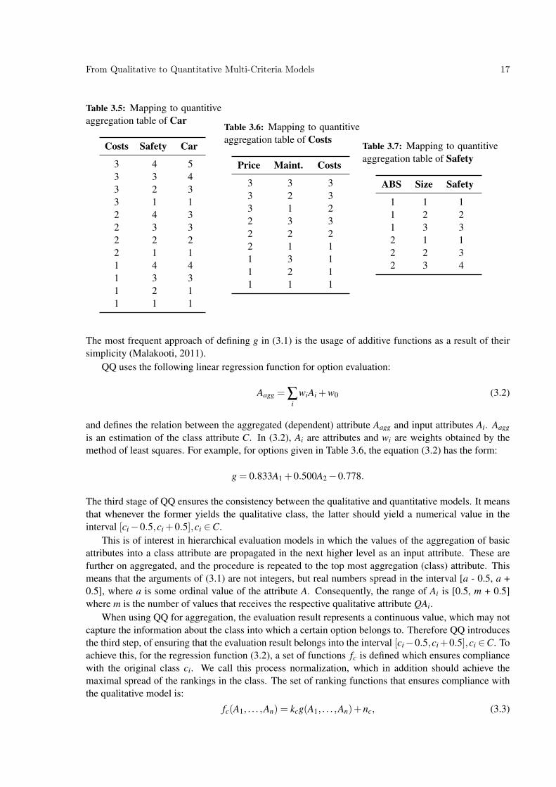
To demonstrate the usage of χ2 for weights calculation, consider the running example given in Ta-ble 2.2. The contingency tables and the values of xi0, x j0 and x00 between A1 and C, and between A2 andC are given with Tables 4.1 and 4.2, respectivlly.
Table 4.1: Contingency table, xi0, x j0 and x00 between a1 ∈ A1 and ci ∈ C for the running example inTable 2.2
x(i,j) c1 = 1 c2 = 2 c3 = 3 x j0
a1 = 1 3 0 0 3a1 = 2 1 1 1 3a1 = 3 0 1 2 3
xi0 4 2 3 x00 = 9
Modifications of QQ with Impurity Functions, Polynomials and Optimization Functions 25
Table 4.2: Contingency table, xi0, x j0 and x00 between a2 ∈ A2 and ci ∈ C for the running example inTable 2.2
x(i,j) c1 = 1 c2 = 2 c3 = 3 x j0
a2 = 1 2 1 0 3a2 = 2 1 1 1 3a2 = 3 1 0 2 3
xi0 4 2 3 x00 = 9.
The values of χ2 are χ21 (A1,C) = 6.5 and χ2
2 (A2,C) = 3.5, which, when normalized, lead to thefollowing weights values in (3.2): ω1 = 0.65 and ω1 = 0.35.
4.1.3 Information Gain
Information gain (IG) has its origin in information theory and it is frequently used in decision tree learn-ing for determining the attribute that gives most information regarding some splitting criteria. It is definedas:
IG(C,A j) = H(C)−p
∑q=1
|ASq|r
H(cq) (4.7)
where C is the class attribute, A j is the jth input attribute, r is the number of options, p is the number ofvalues that the attribute A j may receive, |ASq| is the number of options that receive the same value ASq,cq is the subset of the class attribute for which the attribute A j receives the qth value. The equation (4.7)may be expanded with the equation for entropy H, leading to (Raileanu and Stoffel, 2000):
IG(C,A j) =−m
∑k=1
p(ck) log(p(ck))+p
∑q=1
p(aq)m
∑k=1
p(ck|aq) log(p(ck|aq)) (4.8)
where aq =|ASq|
r , p(ck) is the probability that a randomly selected example belongs to the class ck ∈C,− log(p(ck)) is the information that it conveys with, p(aq) is the probability that the attribute A j willreceive the value ASq, and p(ck|aq) is the conditional probability.
4.1.4 Weights Calculation with Impurity Functions
Each of the explained impurity functions (4.4)–(4.8) are used to calculate the weights in (3.2) (and settingw0 = 0) by applying Algorithm 2.
Algorithm 2 Calculation of weights wi with impurity function
1: for i = 1→ n do . for each input attribute Ai, and class attribute C2: Wi = f (Ai,C) . calculate the value of the impurity function f (Ai,C)3: end for4: wi← norm(Wi) in the interval [0,1] . obtain the weights wi with normalization
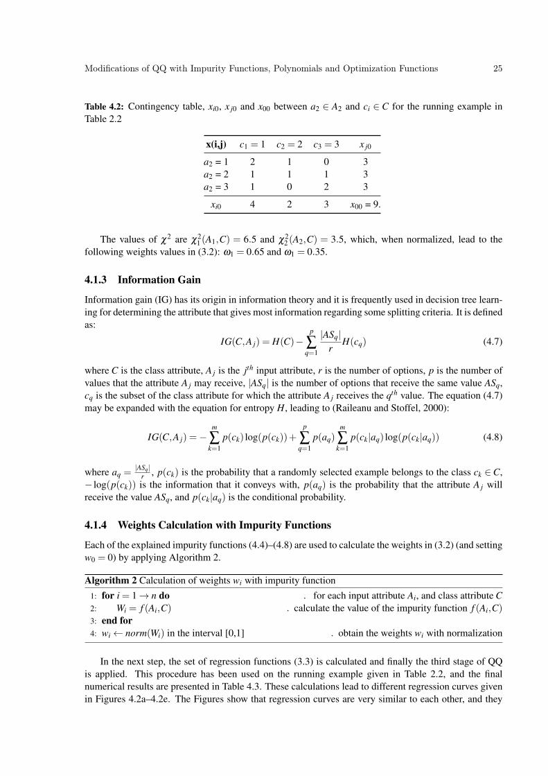
In the next step, the set of regression functions (3.3) is calculated and finally the third stage of QQis applied. This procedure has been used on the running example given in Table 2.2, and the finalnumerical results are presented in Table 4.3. These calculations lead to different regression curves givenin Figures 4.2a–4.2e. The Figures show that regression curves are very similar to each other, and they
26 Modifications of QQ with Impurity Functions, Polynomials and Optimization Functions
differ in the inclination angle. The most dissimilar are the curves obtained using gP approach, givenin Figure 4.2c. Here the regression estimation curve for the second class given in Figure 4.2c providesan inverse rank estimation for the two options belonging in this class in comparison with the rankingsobtained by the rest of the methods. This can be better noticed from the numerical calculations inTable 4.3, where option 6 is better ranked than option 5 only when gP method is used. Both rankings areconsidered as correct in this case, as all conditions for the required method given in Chapter 2 are fulfilled.The example shows that different methods lead to different rankings that can satisfy the requirements.
Table 4.3: Quantitative ranking of options with different impurity functions
No. A1 A2 C gB gC gP IG χ2
1 1 1 1 0.7963 0.7857 0.7420 0.7910 0.79412 2 1 1 1.2037 1.1429 0.9681 1.1640 1.17653 1 2 1 0.9815 1.0000 1.0000 1.0000 1.00004 1 3 1 1.1667 1.2143 1.2580 1.2090 1.20595 3 1 2 2.1364 2.1000 1.9691 2.1099 2.11546 2 2 2 1.8636 1.9000 2.0309 1.8901 1.88467 3 2 3 3.0185 2.9615 2.8262 2.9765 2.98488 2 3 3 2.7963 2.8077 2.8692 2.8047 2.80309 3 3 3 3.2037 3.1923 3.1738 3.1953 3.1970
4.2 Polynomial Models for Regression
The linear regression, introduced in the second stage of QQ, may be replaced with a different formof regression, the polynomial regression. The polynomial regression introduces a regression model ina form of polynomial equation which predicts the value of the dependent variable y. A polynomialregression equation over the attributes A1,A2, . . . ,An can be written as:
y = w0 +m
∑i
wiTi (4.9)
where Ti = ∏nj=1 Aui, j
j , and ui, j ∈ N. Here y is estimation of the class attribute C. To explore the usage ofpolynomial functions for regression in the second stage of QQ, the CIPER machine learning algorithm isused. There are two versions of the CIPER algorithm: CIPER (Todorovski et al., 2004) and New CIPER(Peckov et al., 2008). Both algorithms are explained next.
4.2.1 CIPER
CIPER is an algorithm that uses a specific heuristics to define and search the space of possible polynomialfunctions. As a result it finds one (or several) polynomial function that satisfies the heuristics and thatprovides best fit for the data. The heuristics is given with a set of constraints. In order to define theconstrains, CIPER introduces the following notation for (4.9):
1. length of y is Len(y) = ∑mi=1 ∑
nj=1 ui, j,
2. the size of y (number of terms) is size(y) = m,
3. a degree of a term Ti is Deg(Ti) = ∑nj=1 ui, j and

Modifications of QQ with Impurity Functions, Polynomials and Optimization Functions 27
Attribute 1Attribute 2
Regressioncu
rves
11.5
22.5
3
1
1.5
2
2.5
3
0.5
1
1.5
2
2.5
3
3.5
(a) Gini Breiman
Attribute 1Attribute 2
Regressioncu
rves
11.5
22.5
3
1
1.5
2
2.5
3
0.5
1
1.5
2
2.5
3
3.5
(b) Gini covarianceAttribute 1Attribute 2
Regressioncu
rves
11.5
22.5
3
1
1.5
2
2.5
3
0.5
1
1.5
2
2.5
3
3.5
(c) Gini population
Attribute 1Attribute 2
Regressioncu
rves
11.5
22.5
3
1
1.5
2
2.5
3
0.5
1
1.5
2
2.5
3
3.5
(d) Information gainAttribute 1Attribute 2
Regressioncu
rves
11.5
22.5
3
1
1.5
2
2.5
3
0.5
1
1.5
2
2.5
3
3.5
(e) χ2
Figure 4.2: Regression curves obtained with different weights estimation in QQ
4. degree of y is Deg(y) = maxmi=1Deg(Ti).
In order to search the space of possible polynomial equations using the predefined heuristics, CIPERemploys iterative beam search. The beam may be initialized in two ways: with the simplest polynomialequation or with some user-defined polynomial, that is considered as the minimal one in the beam search.In each iteration a new set of polynomials is generated from the existing polynomials in the beam by usingsome refinement operator.
A refinement operator is a function which takes as input some polynomial structure y and generatesa new one by modifying y. The refinement operator in CIPER modifies y by increasing Len(y) for oneunit. It may be performed in two ways: by adding a new first degree term Ti or by increasing an existingterm with a variable. The coefficients wi in the newly created polynomial equations are calculated usingthe method of least squares.

28 Modifications of QQ with Impurity Functions, Polynomials and Optimization Functions
Each of the generated polynomial equations are evaluated so that the degree of fit of the equationto the given data set is estimated. For evaluation of equations a minimum descriptor length (MDL)heuristics is used. CIPER uses an ad-hoc MDL heuristic given as (Todorovski et al., 2004):
MDL(y) = Len(y) log(k)+ k log(MSE(y)) (4.10)
where MSE(y) is the mean squared error and k is the number of training examples. The first term in(4.10) represents a penalty for the equation complexity, while the second term measures the degree of fitof the equation. More preferred equations are those with smaller MDL.
During the search, CIPER maintains a set of b best possible equations in the beam that satisfy the im-posed constraints. The search finishes when the refinement operator cannot generate any new equationswhose evaluation outperforms the evaluation of the equations that are already kept in the beam.
4.2.2 New CIPER
The New CIPER improves and extends CIPER in following maners:
1. it provides an improved refinement operator,
2. it provides a new MDL Scheme for polynomial regression,
3. it employes error on unseen data as search heuristics.
The New CIPER extends CIPER so that it:
1. learns piecewise polynomial models,
2. is capable for multi-target polynomial regression,
3. performs classification via multi-target regression.
Each of the improvements and extensions are explained.
Improved refinement operator The need for improving the refinement operator is motivated from thefact that when a term is added to a polynomial, it decreases its error. On the other hand, when a term isreplaced with a more complex version, such as a multiplication of the term with a variable, it does notdecrease the error in general. For example, adding A1 to A2 yielding to A1 +A2 would reduce the errorof the equation. However, the replacement of A1 with A1A2 may increase the error of the equation. NewCIPER introduces a third refinement operator, which takes a term in the equation, copy it and multiplyit with the new variable. The obtained term is added to the existing equation. For example, the equationA1+A2 is refined by coping the term A1 and multiplying it with A2. The new term is added to the equationleading to A1 +A2 +A1A2. This refinement operator increases the complexity of the newly generatedpolynomial equation. Therefore, in each step of the algorithm, for the newly generated equation, eachterm is removed and an evaluation of the equation is performed. If the evaluation outperforms the existingequation in the beam, the new equation is added to the beam.
New MDL Scheme for polynomial regression For evaluation of polynomial equations, the NewCIPER uses the following MDL:
MDL(y) = L(y)+2W (y,D)

Modifications of QQ with Impurity Functions, Polynomials and Optimization Functions 29
where L(y) is the number of bits for encoding the polynomial structure, and W is a stochastic complexityof a linear regression model that uses least squares. To calculate L(y), the following equation is used(Peckov et al., 2008):
L(y) = 2log(l)+2log(log(l))+ log |G(n, l)|+ log |G′(u1,u2, . . . ,un)|.
Here l = Len(y), |G(n, l)| is the number of polynomial structures with n terms and length l. The class ofpolynomials that belong to G(n, l) is partitioned into subclasses with fixed term degrees G′(u1,u2, . . . ,un).All polynomials that belong to this subclass have n terms with degrees u1≥ u2≥ ·· ·≥ um. |G′(u1,u2, . . . ,un)|is the number of polynomial structures in G′(u1,u2, . . . ,un).
W is calculated with (Rissanen, 2000):
W = minγ(N− p) log(τ)+ p log(N, R)+(N− p−1) log(
NN− p
)− (p+1)log(p)
where γ is an index that goes though all subsets of variables in the linear regression, N is the size of thedata table, p is the number of elements in γ , τ is the maximum likelihood estimation of the model error,and R = 1
N wT (AT A)w where w = (AT A)−1AT y.
Employing error on unseen data as search heuristics New CIPER introduces additional heuristicsfor evaluation of polynomial models as an alternative to the MDL. It is called CV (cross validation)heuristics. It considers the data set as a training set that is used to build the polynomial model. It splitsthe train set into 10 parts (options), and builds the model on 9 parts. It calculates the square relativeerror on 9 parts obtaining the value of the variable reTrain2, and on the 10th part leading to the valueof reTest2. The procedure of splitting the training set and building a polynomial model is repeatedaccording to a predefined number of times. For each of the modes, the tuple (reTrain2,reTest2) is kept.The beam search is modified so that a derived model with the refinement operator may enter the beamonly if its heuristics value is smaller than min(reTrain2,reTest2).
In the process of generating new polynomial models, an over-fitting may occur. To avoid it, NewCIPER poses a requirement that the reTrain2 should be smaller than reTest2. Otherwise the model isrejected from further refinement. This procedure decreases the probability of over-fitting. As soon as themodels are built, a final model is produced by averaging all built models.
Learning piecewise polynomial models New CIPER introduces the possibility of including piecewisepolynomial models in the beam search. It is designed so that it partitions the space along each attributebefore the the search begins. The partitioning of the attribute’s space is not dependent on the outputattribute (class attribute).
The procedure for partitioning the array of real values A is the following. First, k arrays are obtainedfrom A: A1,A2, . . . ,Ak. For the particular partitioning, a heuristics H is calculated according to:
H(A1,A2, . . . ,Ak) = k(k
∑j=2
(m j−m j−1
2)2 + ∑
x∈A
kminj=1
(x−m j)2) (4.11)
where m j is the mean of the values in A j. The value of (4.11) is compared to the sum of variances:
∑x∈A
(x−mean(A))2. (4.12)
If 4.11 is smaller than (4.12), then the splitting is called possible split with the number k for values in A.For a given k, the best possible split is given with As
1,As2, . . . ,A
sk and it holds:
H(As1,A
s2, · · · ,As
k)≤ H(A1,A2, · · · ,Ak)

30 Modifications of QQ with Impurity Functions, Polynomials and Optimization Functions
for any other partitioning A1,A2, · · · ,Ak of the array A. Next, a function Pk(A) is defined so that it findsthe best partitioning of an array A into k arrays, where k ∈ [2,9]. Hence, Pk(A) chooses an interval (a,b),where b≥ a and a,b ∈ [2,9] so that:
H(Pk(A))≤ H(Pj(A)), for ∀ j = a, . . . ,b.
Pk(A) creates k binary attributes, one for each Asj, j = 2, . . . ,k. This procedure is extended to all attributes.
The obtained binary attributes slice the space. The binary attributes are used for obtaining a piecewisepolynomial model.
The last two extensions of New CIPER include inducing a polynomial equation for prediction ofseveral variables, and introducing of classification by using the induced polynomial structure. Thesewere not of interest here.
CIPER induces the following polynomial on the running example:
C = 0.2903A1 +0.0461A2 +0.1515A1A2 +0.6216. (4.13)
The results from the polynomial (4.13) are given in the last column in Table 4.4 and the regression curveis presented in Figure 4.3.
Table 4.4: Ranking obtained with CIPERfor the running example
No. A1 A2 C CIPER
1 1 1 1 1.10952 2 1 1 1.55143 1 2 1 1.30724 1 3 1 1.50485 3 1 2 1.99326 2 2 2 1.90067 3 2 3 2.49408 2 3 3 2.24989 3 3 3 2.9948
Table 4.5: Ranking obtained with New CIPERfor the running example
No. A1 A2 C New CIPER
1 1 1 1 0.97342 2 1 1 1.61063 1 2 1 1.06304 1 3 1 1.15275 3 1 2 2.21066 2 2 2 1.89617 3 2 3 2.65498 2 3 3 2.18169 3 3 3 3.0992
Attribute 1Attribute 2
Regressionplanes
1
1.5
2
2.5
3
1
1.5
2
2.5
3
0.5
1
1.5
2
2.5
3
3.5
Figure 4.3: Regression curve obtained with CIPER for the running example
By applying New CIPER on the running example, the following polynomial is obtained.
C = 0.4412A1−0.1434A2 +0.2516A1A2−0.0186A21A2 +0.4426. (4.14)

Modifications of QQ with Impurity Functions, Polynomials and Optimization Functions 31
The results from the polynomial (4.14) are given in the last column in Table 4.5, and the regressionfunction is presented in Figure 4.4.
Attribute 1Attribute 2
Regressioncu
rve
1
1.5
2
2.5
3
1
1.5
2
2.5
3
0.5
1
1.5
2
2.5
3
3.5
Figure 4.4: Regression curve obtained with New CIPER for the running example
4.3 Reformulation of the Problem as Optimization Problem with Con-straints
In this section, the ranking problem is reformulated as optimization problem with constraints. The ob-jective is to find a weight vector x, which would minimize the distances between the ranking valuesin-between two consecutive classes. The constrains are given so that ranking values are always in theintervals c±0.5. These constrains eliminate the need of the third stage of QQ. The objective function islinear, hence a linear programming is used to find the solution of the problem.
The general form of the linear programming model is given with:
max f (ω)
subject to gi(ω) = li, for i = 1, · · · ,n Equality constraints
h j(ω)≤ d j, for j = 1, · · · ,m Inequality constraints
ωi ≥ 0
where ω is a vector of decision variables residing in a n-dimensional space, or in this case weights of thelinear objective function, f (ω) is the objective function, and gi(ω) and h j(ω) are constraint functionsthat need to be satisfied, and li and d j are constants (Hillier and Lieberman, 2001). The model may alsoget one of the following forms:
1. The objective function may solve the dual problem of minimization, min f (ω), instead of theprimal problem of maximization;
2. Additional inequality constraints with ‘greater-than-or-equal’ sign: hk(ω)≥ pk for k = 1, · · · ,r;
3. Deleting the non-negativity constraint for some of the decision variables ωi.
The reformulation of the problem of option ranking to an optimization problem is demonstrated onthe running example given in Table 3.6. The Table 3.6 consists of two quantitative attributes and a class.The constraints are defined directly from Table 3.6 as follows. Each row, which may be written in theform of ω1A1 +ω2A2, has to receive an evaluation in the interval ci± 0.5. This is written with twoconstraints:
ω1A1 +ω2A2 ≥ ci−0.5 and ω1A1 +ω2A2 ≤ ci +0.5

32 Modifications of QQ with Impurity Functions, Polynomials and Optimization Functions
The constraints using this formulation are given with (4.15). Next, we have to define the optimizationfunction.
ω1 +ω2 ≥ 0.5,
ω1 +ω2 ≤ 1.5
2ω1 +ω2 ≥ 0.5,
2ω1 +ω2 ≤ 1.5
ω1 +2ω2 ≥ 0.5,
ω1 +ω2 ≤ 1.5
ω1 +3ω2 ≥ 0.5,
ω1 +3ω2 ≤ 1.5
3ω1 +ω2 ≥ 1.5,
3ω1 +ω2 ≤ 2.5
2ω1 +2ω2 ≥ 1.5,
2ω1 +2ω2 ≤ 2.5
3ω1 +2ω2 ≥ 2.5,
3ω1 +2ω2 ≤ 3.5
2ω1 +3ω2 ≥ 2.5,
2ω1 +3ω2 ≤ 3.5
3ω1 +3ω2 ≥ 2.5,
3ω1 +3ω2 ≤ 3.5.
(4.15)
There are two ways to define the optimization function for the running example. The first one is tominimize the distances between border classes and the second one is to maximize the distances betweenborder classes. The maximization of the distances of two neighbouring classes would lead to small differ-ences among options in the class, which is in contrast to the goal of this thesis. Hence the minimizationapproach is used, in order to obtain rankings of options with maximum spread into the intervals ci±0.5where ci ∈C.
The goal is to find the values of ω1 and ω2 that would minimize the distances between the consecutiveclasses. For the running example, we would like to find a function that would rank all options so that itminimizes the sum of the distances between the highest option in one class ci and the lowest in the nexthigher class ci+1.
When defining the objective function, the rankings of the options are unknown, and consequentlythe highest and lowest evaluations of options in classes are also unknown. To solve this problem, wedefine all possible objective functions over the given decision table, and then we search among them forsolution of the defined problem. For example, let us choose that the maximal ranking in the first class ofthe running example is the option number 4, and the minimal ranking in the next higher class, the secondclass, receives option 6. Next, let option 5 receives the maximal ranking in the second class and let uschoose that option 7 receives the minimal ranking in the third class. Then the objective function that is:
min (2ω1 +2ω2)− (ω1 +3ω2)+(3ω1 +2ω2)− (3ω1 +ω2) = min (ω1 +2ω2).

Modifications of QQ with Impurity Functions, Polynomials and Optimization Functions 33
Writing down all possible combinations would lead to the following objective functions:
min 3ω1 +ω2,
min 3ω1
min 3ω1−ω2,
min 3ω1−2ω2
min 2ω1 +2ω2,
min 2ω1 +ω2
min 2ω1−ω2,
min 2ω1
min ω1 +3ω2,
min ω1 +2ω2
min ω1 +ω2,
min ω1
min 3ω2,
min 2ω2
min ω2,
min −ω1 +3ω2
(4.16)
The set of all possible objective functions may be decreased by deleting the functions which are linearcombination of some other function in the set. For example, instead of having two functions min 3ω1 andmin ω1, we may delete the first one and use only the second one in the set of possible objective functions.
Table 4.6: Ranking of options with constraint optimization
No. A1 A2 C Evaluation
1 3 3 3 3.00002 3 2 3 2.50013 3 1 2 2.00024 2 3 3 2.49995 2 2 2 2.00006 2 1 1 1.50017 1 3 1 1.99988 1 2 1 1.49999 1 1 1 1.0000
The next step is to find a solution of the problem defined with any of the objective functions. For thatreason, the implementation of the Simplex algorithm in MATLAB was used. The Simplex algorithm didnot find a solution for any of the defined objective functions that satisfy the constraints 4.15.
For example, the obtained solution from applying the first objective function given in (4.16), min 3ω1+ω2, is provided in Table 4.6.
This solution is proposed by the Simplex solver algorithm in MATLAB as the closest one to theconstraint region of solutions defined by the problem. It does not satisfy the constrains (4.15). Forinstance, the evaluation of option 7 belongs to the interval 2± 0.5, instead of the required interval of1± 0.5. The example shows that the main difficulty of this approach are the stringent constraints thatrarely lead to a solution in the constraint space.

34 Modifications of QQ with Impurity Functions, Polynomials and Optimization Functions
4.4 Implementation of the QQ-Based Algorithms
QQ and its modifications with impurity functions are implemented in MATLAB for a single or hierar-chical setting of decision tables. The optimization approach uses the implemented function for linearprogramming in MATLAB, however a set of functions were developed in order to: automatically defineall constrains and all possible objective functions for a given decision table, and to search among theobjective functions for a solution.
Calculations for CIPER and New CIPER were performed by using the developed tools provided bytheir authors 1. Shell commands were used for iterative calculations of all decision tables covered in thethree sets in Chapter 7. Analysis was performed in MATLAB afterwards for checking the monotonicity,full ranking and consistency of the results.
1CIPER is also available at http://kt.ijs.si/software/ciper/.

35
5 Copula Theory
The main focus of this thesis is the usage of copula-based functions as estimators of the regressionfunction for option ranking. To be able to use copulas, attributes in the decision tables are considered asrandom variables described with their marginal distributions. Copulas are functions which connect themarginal distributions of the random variables and their joint distribution, which is used for regression.In particular, the thesis exploits bi-variate copulas and extend them to multi-variate ones. This is ofessential interest when working with multi-attribute qualitative models. Bi-variate copulas provide thedependencies between two random variables, while multi-variate ones provide the dependancies amongall random variables at hand. To form a multi-variate copula, the bi-variate ones are merged forminga hierarchical copula construction. This chapter presents the basic concepts of probability theory anddescribes all steps required for building a hierarchical copula.
For the obtained hierarchical copula constructions, the thesis presents new quantile regression equa-tions which are given in Chapter 6.
5.1 Basic Concepts of the Probability Theory
Random variables may be discrete or continuous depending on the values they receive. A random vari-able X is discrete, if its set of possible values X is finite, or at mostly, countably infinite. It is uniquelydefined by:
• the set of possible values X ,
• its cumulative distribution function (CDF) or probability density function (PDF).
In continuation, several definitions and theorems are given in order to provide step-by-step formalizationof the theory behind copulas.
Definition 5.1 (Leemis and Park (2005)). A probability density function for a discrete random variableX is a real-valued function f (·) defined for each possible x ∈ X as the probability that X has the value x
f (x) = Pr(X = x).
In addition, f (·) is defined so that∑
x∈Xf (x) = 1.
Definition 5.2 (Leemis and Park (2005)). A probability density function for the continuos random vari-able X is a real-valued function f (·) defined for each x ∈ X as∫ b
af (x)dx = Pr(a≤ X ≤ b),
for any interval (a,b) ∈X . In addition, f (·) is defined so that∫x∈X
f (x)dx = 1.

36 Copula Theory
Definition 5.3. (Leemis and Park, 2005) A cumulative distribution function of the discrete random vari-able X is the real-valued function F(·) defined for each x ∈ X as
F(x) = Pr(X ≤ x) = ∑t≤x
f (t)
where the sum is over all t ∈X , for which t ≤ x.
Definition 5.4. (Leemis and Park, 2005) A cumulative distribution function of the continuos randomvariable X is the continuos real-valued function F(·) defined for each x ∈R as
F(x) = Pr(X ≤ x) =∫
t≤xf (t)dt.
The CDF has the following properties:
• it is strictly increasing: if x1 < x2, then F(x1)< F(x2),
• CDF values belong to the interval [0,1].
Definition 5.5. (Leemis and Park, 2005) Let X be a discrete random variable with CDF F(·). The inversedistribution function (idf) of X is the function F−1 : (0,1)→X defined for all u ∈ (0,1) as
F−1(u) = minx{x : u < F(x)}
where the minimum is over all posible values x ∈ X.
An example of idf F−1(u) of the discrete random variable x is given in Figure 5.1.
x = F!1(u)
a x b0
u
1
Figure 5.1: Inverse distribution function F−1(u)
Theorem 5.1. (Leemis and Park, 2005) Let X be an integer-valued random variable with X = {a,a+1, ...,b} where b may be ∞ and let F(·) be the CDF of X. For any u∈ (0,1), if u < F(a) then F−1(u) = a,else F−1(u) = x where x ∈X is the (unique) possible value of X for which F(x−1)≤ u < F(x).
Theorem 5.2. (Probability integral transformation) If X is a discrete (continuous) random variable withidf F−1(·) and the continuos random variable U is U(0,1) and Z is the discrete (continuous) randomvariable defined by Z = F−1(U) then Z and X are identically distributed.
Here U(0,1) stands for uniform distribution on the interval [0,1]. An example of the theorem 5.2is given in Figure 5.2. In Figure 5.2, the random variable X and the random variable Z obtained withthe probability integral transformation of a random variable U with uniform distribution, share the samenormal distribution N (µ,σ).
Multi-criteria decision models deal with more than one attribute, therefore, we need to define therelations that may exist between different attributes. In probability theory, the relation between randomvariables is determined with their joint distribution function.

Copula Theory 37
F (x)
f(x)
U(0, 1)
Z = F−1(u)
x
-10 -5 0 5 100
0.1
0.2
0
0.2
0.4
0.6
0.8
1
Figure 5.2: Probability integral transform of a random variable X with PDF f (x) and CDF F(x)
Definition 5.6. A joint (two-dimensional) distribution function H(x,y) of two random variables X and Yis given with H(x,y) = Pr(X ≤ x,Y ≤ y).
The function H(x,y) maps H : [0,1]× [0,1]→ [0,1], and it has the following properties:
• H(∞,∞) = 1 and H(−∞,y) = H(x,−∞) = H(−∞,−∞) = 0
• H(x1,y1)−H(x1,y2)−H(x2,y1)+H(x2,y2)≥ 0, ∀ x1 ≤ x2,y1 ≤ y2.
5.2 Quantile Regression
Quantile regression is a tool for performing statistical regression when there is vague or no knowledgeof the relationship among the random variables. It models the relation between specific quantiles of theregression variable and a set of independent variables. The difference between the linear and quantileregression is that the linear regression coefficients represent the increase (decrease) of the regressionvariable produced by increase (decrease) in the independent variables associated with their coefficients.The quantile regression estimates the change in a specified quantile of the regression variable producedby a change in the independent variables (Despa, 2007).
Definition 5.7. A quantile q ∈ [0,1] is a value which divides the distribution F(x) so that there is a givenproportion of observations below the quantile:
F−1(q) = in f{x : F(x)≥ q}.
In case when the quantile in the regression equation is q = 0.5, a median is obtained. The medianrepresents a central value of the distribution, so that half of the data points are less than or equal to it andhalf are greater than or equal to it. The advantage of using median regression as a measure of centre,compared to the mean regression that is obtained when using the least-square algorithm, is due to itsability to resist the strong effect of outliers (Walters et al., 2006).

38 Copula Theory
The need of joint distribution functions for performing regression To define the regression func-tion (3.2), a copula-based approach is used. When using copulas, attributes Ai are regarded as randomvariables. When attributes and options are given in a decision table, we have at hand a sample of joint be-havior of the attributes for which we can also estimate their marginal distributions Fi(Ai). For determiningthe dependences among the random variables, we need to find their joint distribution F(A1, . . . ,An,Aagg)in the unseen space of options. In order to estimate the multi-variate joint densities with a constant esti-mation accuracy, the required sample size rapidly increases with the number of dimensions (Silverman,1986). As we deal with small sample sizes, we adopt the copula approach for estimation of the jointdensity and distribution. Having defined the joint distribution function and the marginals of each randomvariable, we may proceed with the regression task in the probability space.
5.3 Copula Functions
By definition, for two random variables X and Y , which are defined on the same probability space, thejoint distribution function H(x,y) defines the probability of events defined in terms of both X and Y .Finding the joint distribution function in an explicit form is a difficult task. Sklar (1973, 1996) provedthat the joint distribution function H(x,y) of two random variables is equal to the copula C(u,v).
Theorem 5.3. (Sklar’s theorem) Let H be a two-dimensional distribution function with marginal distri-bution functions FX1 and FX2 . Then a copula C(u,v) exists that for all x1,x2 ∈R2,
H(x1,x2) =C(u,v) (5.1)
where u = FX1(x1) and v = FX2(x2). Moreover, if FX1 and FX2 are continuos, then C(u,v) is unique. Oth-erwise C(u,v) is uniquely determined on the Cartesian product Range(FX1) × Range(FX2). Conversely, ifC(u,v) is a copula and FX1 and FX2 are distribution functions then H is a two–dimensional distributionfunction with marginals FX1 and FX2 .
From Theorem 5.3 it follows that, in order to use (5.1), the theorem 5.2 is fundamental for usage ofcopulas. For example, let consider a vector of two random variables (X1,X2), each one with marginalcdfs F1(X1) = Pr(X1 ≤ x1) and F2(X2) = Pr(X2 ≤ x2). Applying theorem 5.2 to each of the componentsof the vector, leads to (U1,U2) = (F1(X1),F2(X2)). Finally, the copula of (X1,X2) is defined as the jointcumulative distribution function of (U1,U2):
C(u1,u2) = Pr(U1 ≤ u1,U2 ≤ u2).
In the thesis, we use copulas as aggregation functions, which map from the unit m-interval [0,1]m to theunit interval [0,1].
Copulas are bound with the Fréchet-Hoeffding bounds (Durante and Sempi, 2010):
max(u+ v−1,0)6C(u,v)6 min(u,v),∀u,v ∈ [0,1] (5.2)
where
u = F1(X1), u∼ U(0,1),
v = F2(X2), v∼ U(0,1),
and
M(u,v)≡max(u,v),
W (u,v)≡min(u,v)

Copula Theory 39
where U(0,1) is uniform distribution on the interval [0,1], and M(u,v) and W (u,v) are called the max-imum and the minimum copula, respectively. Thus copulas lie between these two extremes. They havethree specific properties:
Property 1 C(1,v) =C(v,1) = v, ∀v ∈ [0,1]
Property 2 C(u,v) = 0, if u = 0 and/or v = 0
Property 3 C(u1,v1)−C(u1,v2)−C(u2,v1)+C(u2,v2)≥ 0 holds whenever u1 ≥ u2 and v1 ≥ v2.
The first property says that if we know that the marginal probability of one of the variables is one,then the joint probability is the same as the probability of the other variable. The second property saysthat the joint probability is zero if the marginal probability of any variable is zero. The third property,known as 2-increasing property, says that the value of copula function is always non-negative. The lastproperty is of special interest. Therefore, its derivation is given below, by using the following cases:
1. Let us fix the first argument to u1, and let v1 ≥ v2. In this case one obtains
C(u1,v1)−C(u1,v2)≥ 0. (5.3)
Decreasing the fixed argument to a smaller value u2 ≤ u1, while still holds that v1 ≥ v2, results in:
C(u2,v1)−C(u2,v2)≥ 0 (5.4)
Finally, the difference between (5.3) and (5.4) leads to:
C(u1,v1)−C(u1,v2)−C(u2,v1)+C(u2,v2)≥ 0
whenever u1 ≥ u2 and v1 ≥ v2.
2. For the opposite case let us fix the first argument to u1, and v1 ≤ v2. In this case one obtains
C(u1,v1)−C(u1,v2)≤ 0 (5.5)
Decreasing the first argument to a smaller value u2 ≤ u1, while still holds that v1 ≤ v2, results in:
C(u2,v1)−C(u2,v2)≤ 0 (5.6)
Finally, the difference between (5.5) and (5.6) leads to:
C(u1,v1)−C(u1,v2)−C(u2,v1)+C(u2,v2)≥ 0
whenever u1 ≤ u2 and v1 ≤ v2.
The 2–increasing property does not require C(u,v) to be actually increasing in either argument asthe "increasingness" can be negative as well. For example, if C(u,v) = au+ bv where a and b are anyconstants, then C(u,v) is 2-increasing, since the inequality (5.3) holds. So we may fix u, increase v andC(u,v) may decrease, but the inequality (5.3) will still hold. If C(u,v) is increasing in each argumentthen C(u,v) is 2-increasing. The opposite does not hold.
The three properties of copulas ensure that they can be used as functions that link a multidimen-sional distribution to its one-dimensional margins. Therefore they are building blocks for models forconstruction of multi-variate dependence (Berg and Aas, 2009).

40 Copula Theory
5.3.1 Archimedean Copulas and Connection to T-norms
If two random variables x and y are independent, then their joint distribution function is H(x,y) =F(x)G(y). In this case, H(x,y) = Π(u,v) = uv, where Π(u,v) is called the product copula. M(u,v),W (u,v) and Π(u,v) are the three most important copulas, as well as the three most important t-norms. Iftwo random variables are dependent, one may write their joint distribution function as a sum of functionsof its marginal distributions:
ϕ(H(x,y)) = ϕ(F(x))+ϕ(G(y)), (5.7)
where ϕ(·) is called a constructor function (Nelsen, 2006). Depending on the form of ϕ(·), one mayelicit different kinds of copulas. In order for a function ϕ : [0,1]→ [0,∞] to be a constructor function, itmust be:
• continuous,
• strictly decreasing from I = [0,1] to [0,∞] and
• ϕ(1) = 0.
The inverse function of ϕ is ϕ−1, defined in the interval 0 6 t 6 ϕ(0). If ϕ(0) < ∞, then the inversefunction is called pseudo-inverse ϕ [−1]. In terms of copulas (5.7) reads:
ϕ(C(u,v)) = ϕ(u)+ϕ(v),
which leads to:C(u,v) = ϕ
[−1](ϕ(u)+ϕ(v)). (5.8)
Copulas obtained using (5.8) are called Archimedean copulas (Joe, 1997). The usage of Archimedeancopulas is mainly motivated by the following three properties:
• symmetry: C(u1,u2) =C(u2,u1) for all u1,u2 ∈ [0,1];
• associativity: C(C(u1,u2),u3) =C(u1,C(u2,u3)), for all u1,u2,u3 ∈ [0,1];
• if ϕ is the generator, then cϕ is also generator for c > 0.
This dissertation focuses on Frank, Clayton and Gumbel copulas which belong to the family of Archimedeancopulas. These three copulas and their generator functions are given in Table 5.1. The median regressioncurve v based on the different Archimedean copulas is given in the last column of Table 5.1. Details ofestimation of the parameter θ are given in Section 5.3.2.
Table 5.1: Different Archimedean copulas, their generator functions ϕ , borders of θ parameter and valueof regression variable v
Cθ (u,v) ϕθ (t) θ Solve( ∂Cθ (u,v)∂u = q,v)
Clayton[max
(u−θ + v−θ −1,0
)]−1/θ 1θ
(t−θ −1
)[−1,∞)\{0} (1−u−θ +(qu1+θ )−
θ
1+θ )−1θ
Frank − 1θ
ln(
1+(e−θu−1)(e−θv−1)
e−θ −1
)− ln
e−θ t −1e−θ −1
(−∞,∞)\{0} 1θ
log −eθ (1−q+qeθu)−eθ+qeθ−qeθu
Gumbel-Hougaard exp(−[(lnu)θ +(− lnv)θ
]1/θ)
ln1−θ(1− t)
t[1,∞) only numerical solution

Copula Theory 41
PSfrag repla ements
u1u2CDF
00.51
0 0.2 0.4 0.6 0.8 1 00.10.20.30.40.50.60.70.80.91
00.20.40.60.8100.20.40.60.81
Figure 5.3: Clayton copula distributionfunction C(u1,u2)
PSfrag repla ements
u1u2PDF
00.51
0 0.2 0.4 0.6 0.8 1 0.90.9511.051.1
00.20.40.60.8100.140.290.430.570.710.861
Figure 5.4: Clayton copula density function c(u1,u2)
5.3.2 Estimation of the Parameter θ
The PDF and CDF are connected with the derivative (integral) relation. In terms of copulas, the jointCDF is H(x,y) =C(u,v), hence to obtain the joint PDF one uses the relation:
c(u,v) =∂ 2C(u,v)
∂u∂v.
As an example, one may consider the Clayton copula. Starting from its CDF, one gets the densityfunction as:
c(u,v) = (1+θ)(uv)−(θ+1)(u−θ + v−θ −1)−1+2θ
θ
The rearrangment of the last equation leads to:
c(u,v) = (1+θ)(uv)−(θ+1)(u−θ + v−θ −1)−1+2θ
θ (5.9)
The only free parameter when using the Archimedean copulas is θ . One way to find θ in (5.9) is to usethe maximum likelihood estimation. By definition, the likelihood function of a random sample of size nis the joint probability density (mass) function denoted by (Martinez and Martinez, 2002):
L(θ) = L(θ ;x1,x2, ...,xn) = f (x1,x2, ...,xn;θ) (5.10)
where θ is a vector of parameters. In order to estimate θ that maximizes the likelihood function (5.10),we take the derivative of L(θ) with respect to θ and set it equal to zero:
∂L(θ)∂θ
= 0
The function log(L(θ)) varies monotonically with its argument, or in other words, log(L(θ)) increasesand decreases when L(θ) increases and decreases respectively. This is because both functions are mono-tonically related to each other, leading to the same maximum estimate for both functions (Myung, 2003).In other words, the maxima of the likelihood function and the maxima of the logarithm of the likelihoodfunction are the same. We use this fact in cases when it is easier to find the maxima of a logarithmlikelihood function, such as when exponents are involved in the density function, as it is in our case. Thelogarithm of the density function c(u,v) is:
logc(u,v) = log(1+θ)− (θ +1) log(uv)− 1+2θ
θlog(u−θ + v−θ −1)
Finally, θ is determined as the minimum negative log likelihood (Brent, 1993; Forsythe et al., 1976).The same procedure may be applied to all copulas that belong to the Archimedean family.

42 Copula Theory
5.3.3 Interpretation of the Parameter θ
Copulas can help us in studying the dependence association between random variables. For example, onemay use the well-known Kendall’s τ measure of association, which measures the concordance betweenrandom variables. The population version for Kendall’s τ is
τθ = 1+4∫ 1
0
ϕ(t)ϕ(t)′
.
An example, of Kendall’s tau τθ , for different Archimedean copulas is given in Table 5.2. From Table 5.2
Table 5.2: Kendall’s tau (Nelsen, 2006)
Copula Kendall’s tau
Gumbel θ−1θ
Clayton θ
θ+2Frank 1−θ
4 [1−D1(θ)], D1(θ) =1θ
∫θ
0t
et−1 dt
it is clear that the higher values of θ mean higher dependence association between the two randomvariables.
Another measure of dependence is the tail dependence. It is a concept which relates the amount ofdependence in the upper-right quadrant tail or lower-left quadrant tail of a bi-variate distribution. It isa useful concept for studying dependence between extreme values. The Gumbel copula has upper taildependence λu given with Rachev (2003):
λu = 2−21θ .
Clayton copula does not have upper tail dependence, however it has a lower tail dependence λL givenwith Rachev (2003):
λL = 2−1θ .
The Frank family of copulas does not have upper nor lower tail dependence.
5.4 Higher-Dimensional Copulas
Quantitative models generally consist of more than two attributes. In order to use the described bi-variate copulas in multi attribute models, one needs to extend them to higher dimensions. There are twoapproaches of extending to higher dimensional copulas (Fischer et al., 2009; Savu and Trade, 2006):
1. The first approach extends the bi-variate copula to multi-variate copula using only one dependenceparameter θ to specify the dependences among n random variables. Such copulas are known asexchangeable Archimedean copulas (Berg and Aas, 2009; Hofert, 2008). In this case the copulafunctions and the joint distribution function are related with the relation:
H(x1, . . . ,xn) =C(u1, . . . ,un;θ).
Their main drawback is that copula densities for dimensions higher than two are tedious to derive(Trivedi and David, 2006);

Copula Theory 43
2. The second approach uses bi-variate copulas to form a hierarchical structure with at most n−1 dependence parameters θi for n random variables. There are two possibilities to build suchhierarchical structures (Berg and Aas, 2009): the FNAC, as shown in Figure 5.5, and the PNAC,as shown in Figure 5.7.
For a given decision table, the described two approaches can be used as follows:
1. Symmetric decision tables are aggregated with the first approach, which uses only one dependenceparameter θ . This approach ensures the symmetry in the evaluations of options.
2. Partially symmetric decision tables are aggregated in two-step procedure. In the first step, eachgroup of symmetric attributes is aggregated with one parametric copula. In the second step, thenon-symmetric attributes and the formed copulas are aggregated either with one parametric or withmulti parametric copula.
3. Non-symmetric decision tables are aggregated either with one parametric or with multi parametriccopula (FNACs or PNACs).
5.4.1 One-Parametric Archimedean Multi-Variate Copulas
Multivariate Archimedean copulas are given with:
C(u1,u2, . . . ,ud) = ϕ[−1](ϕ(u1)+ϕ(u2)+ . . .+ϕ(ud), (5.11)
where ϕ is a generator function with single parameter θ . In the 3-dimensional case, (5.11) is givenwith:
C(u1,u2,u3) = ϕ[−1](ϕ ◦ϕ
[−1](ϕ(u1)+ϕ(u2))+ϕ(u3)) =C(C(u1,u2),u3).
The simbol ◦ stands for composite functions. It means that the argument of the function standing beforethe simbol ◦ is the outcome of the function after the simbol ◦.
Similarly, one may show that:
C(u1,u2,u3) =C(u1,C(u2,u3)) =C(C(u1,u2),u3) =C(C(u1,u3),u2).
In other words, the one-parametric Archimedean copula may be written as a structure of nested bi-variatecopulas with the same value of the parameter θ .
To estimate θ in (5.11), we use the maximum-likelihood approach. For that purpose one needs tocalculate the corresponding probability density c(u1,u2, . . . ,ud). The general form of the copula densityexpressed through the generator function is:
c(u1,u2, . . . ,ud) = ϕ−1(d)(ϕ(u1)+ϕ(u2)+ . . .+ϕ(ud))
d
∏i=1
ϕ′(ui)
where ϕ−1(d) denotes the d-th derivative of the inverse generator function.The canonical loglikelihood function is
lnL(θ ;uit , i = 1, . . . ,d, t = 1, . . . ,T ) =T
∑t=1
lncL(u1t , . . . ,udt ;θ) (5.12)
where d is number of attributes, t is number of observations (options), and the canonical maximumlikelihood estimator of θ is
θ = argmaxlnL(θ). (5.13)
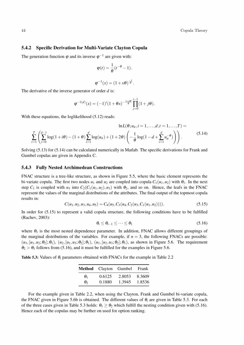
44 Copula Theory
5.4.2 Specific Derivation for Multi-Variate Clayton Copula
The generation function ϕ and its inverse ϕ−1 are given with:
ϕ(t) =1θ(t−θ −1).
ϕ−1(x) = (1+ xθ)
−1θ .
The derivative of the inverse generator of order d is:
ϕ−1(d)(x) = (−1)i(1+θx)−
1+dθ
θ
i−1
∏j=0
(1+ jθ).
With these equations, the loglikelihood (5.12) reads:
lnL(θ ;uit , i = 1, . . . ,d, t = 1, . . . ,T ) =T
∑t=1
(d−1
∑i=0
log(1+ iθ)− (1+θ)d
∑i=1
log(uit)+(1+2θ)
(− 1
θlog(1−d +
d
∑i=1
u−θ
it )
)).
(5.14)
Solving (5.13) for (5.14) can be calculated numerically in Matlab. The specific derivations for Frank andGumbel copulas are given in Appendix C.
5.4.3 Fully Nested Archimedean Constructions
FNAC structure is a tree-like structure, as shown in Figure 5.5, where the basic element represents thebi-variate copula. The first two nodes u1 and u2 are coupled into copula C1(u1,u2) with θ1. In the nextstep C1 is coupled with u3 into C2(C1(u1,u2),u3) with θ2, and so on. Hence, the leafs in the FNACrepresent the values of the marginal distributions of the attributes. The final output of the topmost copularesults in:
C(u1,u2,u3,u4,u5) =C4(u5,C3(u4,C2(u3,C1(u1,u2)))). (5.15)
In order for (5.15) to represent a valid copula structure, the following conditions have to be fulfilled(Rachev, 2003):
θi ≤ θi−1 ≤ ·· · ≤ θ1 (5.16)
where θ1 is the most nested dependence parameter. In addition, FNAC allows different groupings ofthe marginal distributions of the variables. For example, if n = 3, the following FNACs are possible:(u3, [u1,u2;θ2];θ1), (u2, [u1,u3;θ2];θ1), (u1, [u2,u3;θ2];θ1), as shown in Figure 5.6. The requirementθ2 > θ1 follows from (5.16), and it must be fulfilled for the examples in Figure 5.6.
Table 5.3: Values of θi parameters obtained with FNACs for the example in Table 2.2
Method Clayton Gumbel Frank
θ1 0.6125 2.8053 8.3609θ2 0.1880 1.3945 1.8536
For the example given in Table 2.2, when using the Clayton, Frank and Gumbel bi-variate copula,the FNAC given in Figure 5.6b is obtained. The different values of θi are given in Table 5.3. For eachof the three cases given in Table 5.3 holds: θ1 ≥ θ2 which fulfill the nesting condition given with (5.16).Hence each of the copulas may be further on used for option ranking.

Copula Theory 45
Figure 5.5: Fully nested Archimedean constructions of multi-dimensional copulas
(a) First permutation (b) Second permutation (c) Third permutation
Figure 5.6: Three permutations of the input variables
5.4.4 Partially Nested Archimedean Constructions
Another approach to obtain a hierarchical structure of Archimedean copulas is by plugging in bi-variateArchimedean copulas into each other, which leads to structures known as partially nested Archimedeancopulas (PNAC). PNACs are more complex structures than FNACs and are found useful when it is notpossible to build FNAC due to the constraints (5.16).
Two examples of PNACs for a decision problem with four attributes and an output class are presentedin Figure 5.7. In order for the PNAC to represent a copula itself, the general condition is that parametersθi must decrease with the level of nesting, while there are no constraints on their values when two or morecopulas are built on the same level (details are given in Section 5.4.5). Consequently, for the copula givenin Figure 5.7a, the following nesting conditions must hold:
θ2 ≤ θ11, θ2 ≤ θ12, θ3 ≤ θ2,
while regarding the copula given in Figure 5.7b the following must be fulfilled:
θ2 ≤ θ11, θ3 ≤ θ12, θ3 ≤ θ2. (5.17)

46 Copula Theory
u1
C1,1(u1,u2;θ11)
C2(C1,1,C1,2;θ2)
u2 u3 u4
C1,2(u3,u4;θ12)
C3(C2,u5;θ1)
u5
(a) First PNAC
u1
C1,1(u1,u2;θ11)
C2(C1,1,u3; θ2)
u2 u3 u4
C1,2(u4,u5;θ12)
C3(C2,C1,2;θ1)
u5
(b) Second PNAC
Level 1
Level 2
Level 3
Input level
Figure 5.7: Partially nested Archimedean constructions with five attributes
5.4.5 Conditions for FNAC and PNAC
In this section, an explanation of the origin of equations (5.16) and (5.17) is provided. In order for Cn torepresent a valid n - dimensional FNAC or PNAC, the inverse of ϕ in (5.7), the ϕ−1, must be completelymonotone on the interval [0,∞] as given in (Rachev, 2003, Theorem 6.8). In order for a function tobe completely monotone on an interval, it must have derivatives of all orders which alternate in sign(Rachev, 2003, Definition 6.2). The inverse generator function for the Clayton copula is:
ϕ−1(t) = (θ t +1)−1/θ
In each level n ≥ 2, the argument into the inverse generator function ϕ−1i+1 is the generator function ϕi
from the previous level, leading to composite generator functions:
ϕ(t) = ϕi ◦ϕ−1i+1(t) =
((θi+1t +1)−1
θi+1 )−θi−1θi
(5.18)
where i is the level in the FNAC or PNAC. In order to get a valid hierarchical copula, the compositefunctions must fulfill
(−1) j−1(ϕi ◦ϕ−1i+1)
( j)(t)≥ 0 (5.19)
as described in (Rachev, 2003). Next, if we find the derivatives of (5.18) we get:
ϕ(1)(t) = (θi+1t +1)
θi−θi+1θi+1
ϕ(2)(t) = (θi−θi+1)(θi+1t +1)
θi−2θi+1θi+1
ϕ(n)(t) = (θi−θi+1)(θi−2θi+1)...(θi− (n−1)θi+1)(θi+1t +1)
θi−nθi+1θi+1 (5.20)
In order (5.20) to fulfill (5.19), the nesting condition (5.16) has to be fulfilled, which here receivesthe form: θi+1 ≥ θi.
The same may be applied for Gumbel (Rachev, 2003, Example 6.13) and Frank copulas.Here we should note that the Fréchet-Hoefding inequality (5.2) bounds the values of the hierarchical
copula in such a way that, whenever adding one more level in the FNAC or PNAC, the resulting copulawill be smaller or in best case equal to the previous one. In other words, in each level of copula construc-tion, the bounds of the resulting inverse cumulative function will become closer to each other and closerto the lower output class.
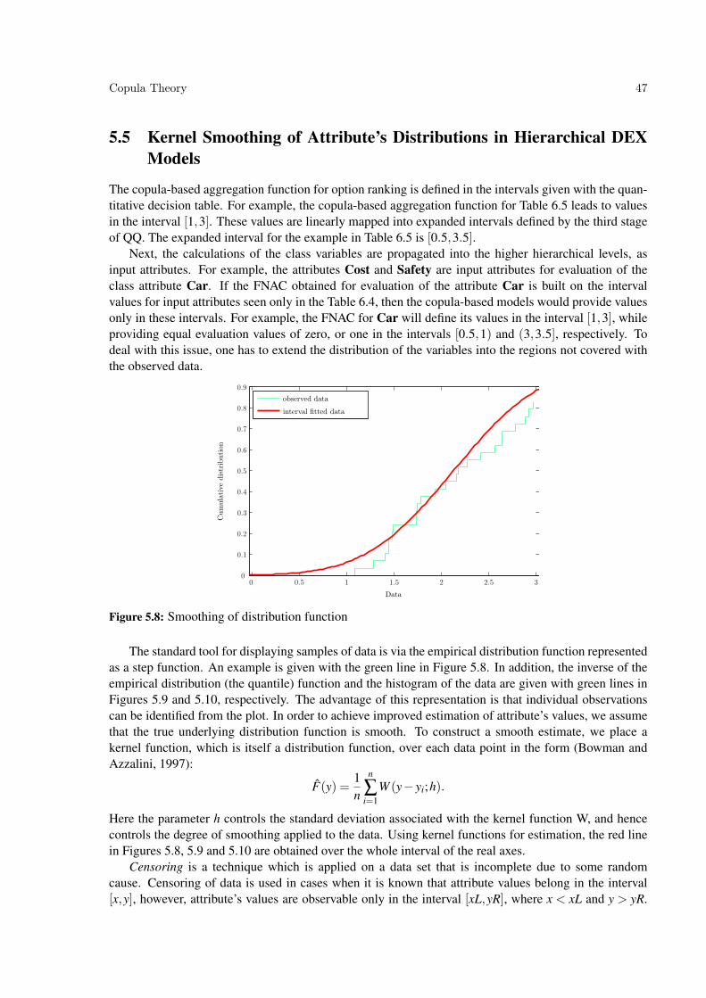
Copula Theory 47
5.5 Kernel Smoothing of Attribute’s Distributions in Hierarchical DEXModels
The copula-based aggregation function for option ranking is defined in the intervals given with the quan-titative decision table. For example, the copula-based aggregation function for Table 6.5 leads to valuesin the interval [1,3]. These values are linearly mapped into expanded intervals defined by the third stageof QQ. The expanded interval for the example in Table 6.5 is [0.5,3.5].
Next, the calculations of the class variables are propagated into the higher hierarchical levels, asinput attributes. For example, the attributes Cost and Safety are input attributes for evaluation of theclass attribute Car. If the FNAC obtained for evaluation of the attribute Car is built on the intervalvalues for input attributes seen only in the Table 6.4, then the copula-based models would provide valuesonly in these intervals. For example, the FNAC for Car will define its values in the interval [1,3], whileproviding equal evaluation values of zero, or one in the intervals [0.5,1) and (3,3.5], respectively. Todeal with this issue, one has to extend the distribution of the variables into the regions not covered withthe observed data.
Data
Cum
ula
tiv
edis
trib
utio
n
observed data
interval fitted data
0 0.5 1 1.5 2 2.5 30
0.1
0.2
0.3
0.4
0.5
0.6
0.7
0.8
0.9
Figure 5.8: Smoothing of distribution function
The standard tool for displaying samples of data is via the empirical distribution function representedas a step function. An example is given with the green line in Figure 5.8. In addition, the inverse of theempirical distribution (the quantile) function and the histogram of the data are given with green lines inFigures 5.9 and 5.10, respectively. The advantage of this representation is that individual observationscan be identified from the plot. In order to achieve improved estimation of attribute’s values, we assumethat the true underlying distribution function is smooth. To construct a smooth estimate, we place akernel function, which is itself a distribution function, over each data point in the form (Bowman andAzzalini, 1997):
F(y) =1n
n
∑i=1
W (y− yi;h).
Here the parameter h controls the standard deviation associated with the kernel function W, and hencecontrols the degree of smoothing applied to the data. Using kernel functions for estimation, the red linein Figures 5.8, 5.9 and 5.10 are obtained over the whole interval of the real axes.
Censoring is a technique which is applied on a data set that is incomplete due to some randomcause. Censoring of data is used in cases when it is known that attribute values belong in the interval[x,y], however, attribute’s values are observable only in the interval [xL,yR], where x < xL and y > yR.

48 Copula Theory
Cumulative distribution
Quantile
observed data
interval fitted data
0 0.1 0.2 0.3 0.4 0.5 0.6 0.7 0.8 0.9-0.5
0
0.5
1
1.5
2
2.5
3
3.5
Figure 5.9: Smoothing of inverse distribution function
Data
Den
sity
observed data
interval fitted data
0 0.5 1 1.5 2 2.5 3 3.5 40
0.1
0.2
0.3
0.4
0.5
0.6
0.7
Figure 5.10: Smoothing of density function
Different censoring techniques may be found in Topp (2002) (Klein and Moeschberger, 2003). Whensome observations in a sample are censored, a convenient approach to estimating the distribution functionwith the distinctive feature that the steps are not all of size 1/n. This suggests that in the case of censoreddata a density estimate should be constructed of the form
fc(y) =n
∑i=1
viw(y− yi;h)
where vi denotes the size of the jump at observation yi.

49
6 Regression Using Nested Archimedean Copulas
The aim of this thesis is to provide ranking of qualitative options as described in Chapter 2. As soon asthe qualitative options are mapped into quantitative ones, using the mapping function F : QS→ S, whereS = {(I1,C1), . . . ,(Ik,Ck)}, Ii = [Ai1,Ai2, ...,Ain], the next step is to define the function given with (2.2):
f : (Ii,Ci) ∈ S→ R.
In this thesis different regression functions are used as a solution to finding a suitable analytical formfor the function given with (2.2). Regression task is employed to determine function’s parameters thatwould best model the relation between independent variables (attributes) and the dependent variable (theclass). In this chapter the regression function (2.2) is obtained by employing a copula-based approach.
When using copulas, attributes Ai are regarded as random variables. For each random variable itsmarginal distributions Fi(Ai) are estimated. For determining the dependences among the random vari-ables, one has to find their joint distribution F(A1, . . . ,An,Aagg). In order to estimate the multi-variatejoint densities with a constant estimation accuracy, the required sample size rapidly increases with thenumber of dimensions (Silverman, 1986). As the problem at hand provides only small sample sizes, onepossibility to determine the joint distribution is by employing copula functions.
The final step of using copulas for solving the problem given in Chapter 2 is to derive the regressionfunction. Such a relation will describe the link between the input attributes and the class attribute. Theregression with copulas is performed in a way that we determine the probability density from the jointdistribution by differentiating over the dependent variable (Brown et al., 2005; Wasserman, 2006). Theregression using bi-variate copulas is described in (Bouyé and Salmon, 2002; Nelsen, 2006).
This thesis extends the bi-variate copula-regression algorithm to multi-variate regression using FNACand PNAC in which the dependent variable may be positioned at any leaf in the hierarchical copula (seeFigures 5.5 and 5.7). This approach is demonstrated on Clayton copula, however, the same procedure isused later in the thesis for the results obtained with Frank and Gumbel copulas (see Table 5.1).
To perform regression, first the partial derivative in respect with the dependent variable is obtained:
q =∂C(u,v)
∂u=− 1
θ(u−θ + v−θ −1)−
1+θ
θ (−θu−(1+θ)) = (1+uθ (v−θ −1))−1+θ
θ (6.1)
solving for q ∈ [0;1], where q is the quantile, leads to v:
v = [1−u−θ +(qu1+θ )−θ
1+θ ]−1θ (6.2)
Replacing u with F(x) and v with G(y) (Nelsen, 2006), where F(x) and G(y) are CDFs of the randomvariables x and y leads to:
G(y) = [1−F(x)−θ +(qF(x)1+θ )−θ
1+θ ]−1θ . (6.3)
Finaly, to obtain the different quantile regression curves for the variable Y one needs to find the inverseof (6.3) (Chen, 2005; Koenker, 2005):
y = G−1[(1−F(x)−θ +(qF(x)1+θ )−θ
1+θ )−1θ ] (6.4)

50 Regression Using Nested Archimedean Copulas
Function (6.4) represents one solution for the required function (2.2) in the problem definition given inChapter 2. This way, a non-linear regression is performed, instead of a linear one as in the QQ method.The curve for copula regression depends on the value of θ . Different regression curves that are obtainedwith different values for θ in the Clayton copula are given in Figure 6.1.
PSfrag repla ements
u
v
θ = 0.1
θ = 0.5
θ = 1
θ = 20 0.1 0.2 0.3 0.4 0.5 0.6 0.7 0.8 0.9 100.10.20.30.40.50.60.70.8
Figure 6.1: Copula-based regression curves for different values of θ in (6.2)
6.1 Quantile Regression
The non-linear regression curves (6.4) used for option ranking when using the copula-based approach,may receive different forms based on two parameters in the regression models:
1. the values of the parameters θ and
2. the quantile q.
In the first case, one may fix the quantile q and examine the curves that are obtained for differentvalues of θ in model. Such an example is given in Figure 6.1, where the regression lines are obtainedfor fixed value of q = 0.5, while examining different values for θ in the Clayton copula-based model(6.2). Figure 6.1 shows that when the value of θ increases, the non-linear regression curves approachthe perfect linearity curve (u = v).
In the second case, the values of θ are fixed, and regression curves for different values of the quan-tiles q are presented. The quantile q is a value which divides the distribution F(x) so that there is a givenproportion of observations below the quantile. Such examples with different values of q are given inFigures 6.2–6.5. The provided examples show the quantiles q = 0.1,0.2, ...,0.9 for Clayton and Frankcopula-based regression curves, and q = 0.01,0.05,0.25,0.5,0.75,0.95,0.99 for Gumbel copulas in Fig-ures 6.2–6.5, respectively. The figures illustrate 200 observations for pairs (u,v) and (X ,Y ) representedwith dots, and different curves that represent the corresponding non-linear quantile regression estimatesobtained from bi-variate copulas with the following parameters:
1. Clayton with uniform marginals and θ = 0.7 (Figure 6.2).
2. Frank with Student marginals and two degrees of freedom for: θ = 2.5 (Figure 6.3) and θ =−2.5(Figure 6.4). In the study of several random variables, the distribution function of each one is calleda marginal (Papoulis, 1991). The student-t distribution of a random variable x with n degrees offreedom is given with:
f (x) =γ√
(1+ x2/n)n+1

Regression Using Nested Archimedean Copulas 51
γ =Γ[(n+1)/2]√
πnΓ(n/2)
where Γ(·) is the gamma function:
Γ(n) =∫
∞
0yn−1e−ydy, b >−1
When the argument of gamma function is integer, the function is called generalized factorial dueto Γ(n+1) = nΓ(n) = · · ·= n!, and Γ(1) = 1. The uniform distribution of a random variable x thatreceives values in the interval (x1,x2) is given with:
f (n) ={ 1
x2−x1x1 ≤ x≤ x2
0 otherwise.
3. Gumbel with uniform marginals and θ = 5.7681 (Figure 6.5).
PSfrag repla ements
u
v
0.1 0.2 0.3 0.4 0.5 0.6 0.7 0.8 0.9
0 0.1 0.2 0.3 0.4 0.5 0.6 0.7 0.8 0.9 100.10.20.30.40.50.60.70.80.91
(a)
PSfrag repla ements
X
Y
0.1 0.2 0.3 0.4 0.5 0.6 0.7 0.80.9
-3 -2 -1 0 1 2 3-4-3-2-101234
(b)
Figure 6.2: Clayton qth quantile curves (for q = 0.1,0.2, ...,0.9): (a) for (u,v) and (b) for (X ,Y ) underhypothesis for uniform margins and for θ = 0.7
PSfrag repla ements
u
v
0.1 0.2 0.3 0.4 0.5 0.6 0.7 0.8 0.9
0 0.1 0.2 0.3 0.4 0.5 0.6 0.7 0.8 0.9 100.10.20.30.40.50.60.70.80.91
(a)
PSfrag repla ements
X
Y
0.1 0.2 0.3 0.4 0.5 0.6 0.7 0.8 0.9
-3 -2 -1 0 1 2 3-5-4-3-2-1012345
(b)
Figure 6.3: Frank qth quantile curves (for q = 0.1,0.2, ...,0.9): (a) for (u,v) and (b) for (X ,Y ) underhypothesis for Student margins with two degrees of freedom and for θ = 2.5

52 Regression Using Nested Archimedean Copulas
PSfrag repla ements
u
v
0.10.20.30.40.50.60.70.80.9
0 0.1 0.2 0.3 0.4 0.5 0.6 0.7 0.8 0.9 100.10.20.30.40.50.60.70.80.91
(a)
PSfrag repla ements
X
Y
0.10.20.30.40.50.60.70.80.9
-3 -2 -1 0 1 2 3-5-4-3-2-1012345
(b)
Figure 6.4: Frank qth quantile curves (for q = 0.1,0.2, ...,0.9): (a) for (u,v) and (b) for (X ,Y ) underhypothesis for Student margins with two degrees of freedom and for θ =−2.5
PSfrag repla ements
u
v
0.01 0.05 0.25 0.5 0.75 0.95 0.99
0 0.1 0.2 0.3 0.4 0.5 0.6 0.7 0.8 0.9 100.10.20.30.40.50.60.70.80.91
(a)
PSfrag repla ements
X
Y
0.01 0.05 0.25 0.5 0.75 0.95 0.99
-3 -2 -1 0 1 2 3-5-4-3-2-1012345
(b)
Figure 6.5: Gumble qth quantile curves (for q = 0.01,0.05,0.25,0.5,0.75,0.95,0.99): (a) for (u,v) and(b) for (X ,Y ) under hypothesis for uniform margins and for θ = 5.7681
PSfrag repla ements
u
0.36614
0.366140.46216
0.462160.55819
0.558190.654210.65421
0.65421 0.654210.750240.75024
0.75024 0.750240.84626 0.846260.846260.846260.94229 0.942290.942290.94229
1.0383 1.0383 1.03831.03831.03831.0383
1.13431.13431.13431.1343
1.1343 1.13431.23041.2304
1.2304 1.23041.3264
1.32641.4224
1.42241.5184
1.51841.6145
1.61451.7105
1.71051.8065
1.8065
v
0.1 0.2 0.3 0.4 0.5 0.6 0.7 0.8 0.90.10.20.30.40.50.60.70.80.9
(a)
PSfrag repla ements
u
0.36658
0.366580.4627
0.46270.55882
0.558820.654940.65494
0.65494 0.654940.751060.75106
0.75106 0.751060.84718 0.847180.847180.84718 0.9433 0.94330.94330.94331.0394 1.0394 1.03941.03941.03941.0394 1.1355
1.13551.13551.13551.1355 1.13551.23171.2317
1.2317 1.23171.3278
1.32781.4239
1.42391.52
1.521.6161
1.61611.7123
1.71231.8084
1.8084
v
0.1 0.2 0.3 0.4 0.5 0.6 0.7 0.8 0.90.10.20.30.40.50.60.70.80.9
(b)
Figure 6.6: Frank copula contours curves: (a) for θ = −2.25 and (b) for θ = 2.25 under hypothesis forStudent margins with two degrees of freedom

Regression Using Nested Archimedean Copulas 53PSfrag repla ements
u
v
0 0.1 0.2 0.3 0.4 0.5 0.6 0.7 0.8 0.9 100.10.20.30.40.50.60.70.80.91
Figure 6.7: Clayton copula contours curves forθ = 5.7 under hypothesis for uniform margins
PSfrag repla ements
u
v
0.1 0.2 0.3 0.4 0.5 0.6 0.7 0.8 0.90.10.20.30.40.50.60.70.80.9
Figure 6.8: Gumbel copula contours curves forθ = 5.7 under hypothesis for uniform margins
In each of the examples in the second case, different values of θ are used to provide difference inthe visibility of the examples. In Figure 6.4, a negative value for θ is provided that leads to decreasingregression curves, unlike all other cases with increasing regression curves for positive values of θ .
The contour curves for the Frank, Clayton and Gumbel copulas are given in Figures 6.6, 6.7 and 6.8respectively. The values on the curves represent the calculated values of the copulas in each of the cases.
6.2 Regression with FNAC: Different Positions of Dependent Variable inthe Input Level in the FNAC
Equation (6.4) holds for bi-variate copulas or for a FNAC where the dependent variable enters the con-struction last, such as u5 in Figure 5.5. For such a case, the left hand side of the FNAC can be regarded asa single variable that enters the top-most bi-variate copula together with the dependent variable. There-fore the dependent variable value can be determined as (6.4) for Clayton copula. In cases when such aFNAC breaches the conditions (5.16), one has to rearrange the order in which variables enter the FNAC.The rearranging of the order is possible since the joint distribution function is invariant on the order ofthe variables. Consequently, by rearranging the order in which the variables enter the FNAC, one canensure that the resulting FNAC fulfills the condition (5.16).
To solve the regression task in this case, first a FNAC has to be obtained that fulfills the condition(5.16). Afterwards, the regression part is solved as an iterative procedure starting from the highest levelof FNAC and descending down to the level which contains the dependent variable by substituting thecorrect quantities in (6.2). In each of the iterations, the value of q in (6.2) is substituted with a vector ofregression values obtained from the previous iteration procedure.
The final regression function for obtaining the values of the dependent variable has different formsdepending on the position i in the FNAC with n attributes. For example, for the Clayton FNAC, theregression function reads:
ui =
[1− v−θ +
(qv1+θ
)− θ
1+θ
]− 1θ
i = n[1−C−θi−1
i−2 +(
vi+1C−1+θi−1i−2
) θi−11+θi−1
]− 1θi−1
i ∈ {3, ...,n−1}[1−u−θ1
j +(
v3u−1+θ1j
)− θ11+θ1
]− 1θ1
i, j = 1,2, i 6= j.
(6.5)

54 Regression Using Nested Archimedean Copulas
Here and in section 6.3, the position of the variable in the FNAC and PNAC is denoted with i or j andshould not be confused with the order of the attributes in both hierarchical constructions. The positionis determined with counting starting from the leftmost input variable in the FNAC and PNAC, and goingto the rightmost variable. For the example given in Figure 5.6 in the middle position, the position ofthe output variable is 2, while the output variable at this position is u3 having a subscript 3. Further on,the equations in the thesis are derived regarding the positions in the FNAC and PNAC, while for theexamples, these values have to be adopted to the names of the real variables.
6.3 Regression with PNAC: Case of Four and Five Attributes and Gener-alization to n Attributes
The second type of hierarchical copula structures that are used in this thesis are PNAC. The smallestPNAC may be formed with four attributes.
In the PNAC with four attributes, for example the copula C2(C1,1,C1,2;θ2) formed with u1 - u4 inFigure 5.7a, the regression function depending on the position i, and based on the Clayton bi-variatecopula, reads:
ui =
[1−u−θk
j +(
vu−1+θkj
)− θk1+θk
]− 1θk
,v =[
1− vs−θr +
(vpvs
1+θr)− θr
1+θr
]− 1θr
, (6.6)
where
(k,vs,r,vp) =
{k = 1,vs =C2,r = 3,vp = q for i, j = 1,2, i 6= j,k = 2,vs =C1,r = 3,vp = q for i, j = 3,4, i 6= j.
When PNAC is formed with five attributes, there are two possible constructions as given in Figure 5.7.For PNAC with five attributes, as the one shown in Figure 5.7a, the regression function has two
possible forms:
1. when the dependent variable positioned at u5, the regression form is given with:
u5 =
[1−C2
−θ3 +(
qC2−1+θ3
)− θ31+θ3
]− 1θ3
. (6.7)
2. For other positions ui, i ∈ {1,2,3,4}, the regression equation is given with (6.6) where:
(k,vs,r,vp) =
{(11,C12,2,v), where v(vs,r,vp) = v(u5,3,q) for i, j = 1,2, i 6= j,(12,C12,2,v), where v(vs,r,vp) = v(u5,3,q) for i, j = 3,4, i 6= j.
In case of a PNAC with five attributes as the one shown in Figure 5.7b, the regression equation isgiven with (6.6) where:
(k,vs,r,vp) =
(11,u3,2,v), where v(vs,r,vp) = v(C12,1,q) for i, j = 1,2, i 6= j,(11,C11,2,v) where v(vs,r,vp) = v(C12,1,q) for i = 3 and u j =C11,
k = 12,vs =C2,r = 1,vp = q for i, j = 4,5, i 6= j.

Regression Using Nested Archimedean Copulas 55
The mathematical reasoning The mathematical reasoning of these equations is the following. Fora PNAC that consists of four attributes, for example the copula C2(C1,1,C1,2;θ2) formed with u1 - u4in Figure 5.7a, and the dependent variable ui, where i ∈ 1,2, the regression function gets the followingform:
ui =
[1−u−θ11
j +(
vu−1+θ11j
)− θ111+θ11
]− 1θ11
, i, j = 1,2, i 6= j
where
v =
[1−C2
−θ3 +(
qC21+θ3
)− θ31+θ3
]− 1θ3
.
When the dependent variable is ui, where i ∈ 3,4, the regression function reads:
ui =
[1−u−θ12
j +(
vu−1+θ12j
)− θ121+θ12
]− 1θ12
, i, j = 3,4, i 6= j
where
v =
[1−C1
−θ3 +(
qC11+θ3
)− θ31+θ3
]− 1θ3
.
In case of a PNAC with five attributes as the one shown in Figure 5.7a, the regression function getsone of the two following forms.
For PNAC with five attributes, as the one shown in Figure 5.7a, the regression function has twopossible forms:
1. In case the dependent variable is u5, the regression form is (6.7), which is obtained from (6.2) bysubstituting the appropriate labels.
2. When the dependent variable is ui where i ∈ 1,2, the regression function is:
ui =
[1−u−θ11
j +(
v1u−1+θ11j
)− θ111+θ11
]− 1θ11
, i, j = 1,2, i 6= j (6.8)
where
v1 =
[1−C12
−θ2 +(
v2C121+θ2
)− θ21+θ2
]− 1θ2
and
v2 =
[1−u5
−θ3 +(
qu51+θ3
)− θ31+θ3
]− 1θ3
(6.9)
Similarly, in case when the dependent variable is ui where i ∈ 3,4, the regression function is:
ui =
[1−u−θ12
j +(
v1u−1+θ12j
)− θ121+θ12
]− 1θ12
, i, j = 3,4, i 6= j (6.10)
where
v1 =
[1−C11
−θ2 +(
v2C111+θ2
)− θ21+θ2
]− 1θ2
and v2 is given with (6.9).

56 Regression Using Nested Archimedean Copulas
In case of a PNAC with five attributes as the one shown in Figure 5.7b, the following forms of theregression functions are possible.
1. If the dependent variable is u1 or u2, the regression function is as given in (6.8), however, the valueof v1 in this case is given with:
v1 =
[1−u3
−θ2 +(
v2u3−1+θ2
)− θ21+θ2
]− 1θ2
where
v2 =
[1−C12
−θ3 +(
v2C12−1+θ3
)− θ31+θ3
]− 1θ3
(6.11)
2. If the dependent variable is u3, the regression function is:
u3 =
[1−C11
−θ2 +(
v2C11−1+θ2
)− θ21+θ2
]− 1θ2
where v2 is given with (6.11).
3. If the dependent variable is u4 or u5, the regression function is given with (6.10) where i, j = 4,5,i 6= j and only the value of v1 changes to
v1 =
[1−C2
−θ3 +(
qC2−1+θ3
)− θ31+θ3
]− 1θ3
.
Generalization of PNACs to n attributes When the number of attributes increases, the number ofpossible combinations of PNACs increases, too. However, the obtained PNACs will consist of subsets ofelements presented in Figure 5.7. Hence the careful combination and repetition of these equations willlead to the required regression functions for all kinds of PNACs regardless of the number of attributes.Additionally, the maximum number of parameters θi that have to be estimated will always be equal tothe number of input attributes.
6.4 Number of Possible FNAC and PNAC Structures
The number of possible FNAC structures is n!2 , where n is the number of variables. The possible combi-
nations of PNACs increases with the number of attributes. However, the obtained PNACs will consist ofsubsets of elements presented in Figure 5.7. Hence the careful combination and repetition of equations(6.5) and (6.6) will lead to the required regression functions for all kinds of PNACs regardless of thenumber of attributes. Additionally, the maximum number of parameters θi that have to be estimated willalways be equal to the number of input attributes. The number of possible full binary trees that may beused for calculating copula functions, as function of the number of its attributes, is given in Table 6.1(Bohla and Lancaster, 2006; Sloane, 2011).

Regression Using Nested Archimedean Copulas 57
Table 6.1: Number of PNAC structures depending on the number of attributes
Number of attributes 2 3 4 5 6 7 8 9 10
Number of trees 1 1 2 3 6 11 24 47 103
6.5 Running Example for Regression Using FNAC
For demonstration of the regression using FNAC, consider the example given in Table 2.2, for whichdifferent FNACs are built and their θi parameters are given in Table 5.3. For this example, the position ofthe attributes in the FNAC is u1,u3,u2, as given in Figure 5.6 (b), where u3 is the variable that is obtainedfrom mapping the class attribute. Therefore, the regression should be performed at this position, leadingto two regression iterations which use (6.5). In the first iteration the value of v3 is calculated using theequation
ui = [1− v−θ +(qv1+θ )− θ
1+θ ]−1θ
where ui = v3, q = 0.5, v = u2 and θ = θ2 = 0.1880 for Clayton-based FNAC. Thus
v3 = [1−u2−0.1880 +(0.5u2
1.1880)− 0.1880
1.1880 ]−1
0.1880
In the second and last iteration, the final regression equation is:
ui = [1−u−θ1j +(v3u−1+θ1
j )− θ1
1+θ1 ]− 1
θ1 (6.12)
where the position of the regression variable is given with i = 2, j = 1 and θ1 = 0.6125. Using (6.12)and substituting ui = u2 with the name of the variable u3 as given in Figure 5.6 in the middle position,leads to
u3 = [1−u−0.61251 +(v3u−0.3875
1 )−0.61251.6125 ]−
11.6125 .
The obtained values for u3 are used for the last step of obtaining the values of the inverse distributionfunction (for example see (6.4)), which are the regression values that are required. The regression valuesare given in Table 6.2, in column Clayton FNAC. The final step in calculation of the regression values
Table 6.2: Quantitative ranking of options
No. A1 A2 C Clayton FNACFNAC Normalized
1 1 1 1 1.4151 0.88762 2 1 1 1.9020 1.29503 1 2 1 1.5744 1.02094 1 3 1 1.6624 1.09455 3 1 2 2.1685 2.20626 2 2 2 2.0604 2.00857 3 2 3 2.3228 3.20358 2 3 3 2.1467 2.90909 3 3 3 2.4062 3.3432
is application of the third stage of QQ. This stage is important because it corrects the inconsistencies

58 Regression Using Nested Archimedean Copulas
that might have occured in the second phase, and leads to consistence between the regression valuesand the original model. One such inconsistency that is solved using this stage, is given with options 5and 8. Namely, option 5 has higher ranking value than option 8, however it belongs to a smaller classthan option 8. This is corrected and the obtained values after application of the third stage are given inTable 6.2, in column FNAC Normalized.
Applying the copula method on the example given in Table 2.2, leads to the regression curves that aregiven in Figure 6.9. Here the regression curves are obtained with calculation of the regression values ofthe FNAC built with Gumbel bi-variate copula for the options in Table 2.2. The contours of the regressioncurves are given in Figure 6.10, respectively.
Attribute 1Attribute 2
Regressioncu
rves
0.5
11.5
2
2.53
3.5
0.51
1.5
22.5
3
3.5
0
1
2
3
4
Figure 6.9: Regression curves obtained with FNAC built with Clayton bi-variate copulas
PSfrag repla ements
Attribute 1
Att
ribu
te2
0.511.522.533.5
0.5 1 1.5 2 2.5 3 3.5
0.511.522.533.50.511.522.533.5
0123024Figure 6.10: Contours of the regression curves given in Figure 6.9.
6.6 Copula-Based Option Ranking Algorithms
The approach of option ranking with copulas is a computationally much more demanding compared withthe approach of option ranking with the linear methods. Therefore the goal of this section is to make thistask more user-friendly by providing the algorithms required for ranking of options.
The copula-based option ranking algorithm is given as Algorithm 3. The algorithm starts with thedistribution estimation of the random variables. Then it checks if the DT consists of symmetric attributes.In case of symmetric DT of random variables (see Definition 2.4 for symmetric DT), the algorithmproceeds with estimation of a one-parametric copula construction. If DT is not symmetric, the algorithmchecks if the DT is partially symmetric. In case of partially symmetric DT (see Definition 2.5 for partiallysymmetric), the algorithm estimates one-parametric copulas for each subgroup of symmetric attributes.Next, a FNAC or PNAC is built from the obtained copulas and the rest of the attributes, if any. In case

Regression Using Nested Archimedean Copulas 59
of non-symmetric DT, the algorithm searches for a valid FNAC or PNAC by using bi-variate copulas.For the obtained copula constructions, a suitable regression function is defined according to (6.1)–(6.6).Next normalization of the results is performed as given with (3.3)–(3.5). Finally full ranking of optionsis checked as defined in (2.4).
Algorithm 3 Implementation algorithm
The process of finding a suitable PNAC or FNAC is presented in Algorithm 4. The tree-like structureof the FNAC has the same form regardless of the number of attributes, in contrast to the diferent tree-likeshapes that the PNAC may receive, and whose number increases with the number of the attributes (seeTable 6.1). Therefore it is less complex to look for a valid FNAC hence the algorithm first searches for avalid FNAC. In case it does not exist, the algorithm continues with a search for a valid PNAC.

60 Regression Using Nested Archimedean Copulas
Algorithm 4 Branching the algorithm for search of a valid hierarchical copula
Find FNAC
or PNAC
Find valid FNAC
Found
copula?
Calculate
regression
depending on
the position
Find PNAC
structures
Find valid
PNAC
Found
copula?
Look for
different copula
functions
Perfrom
regression depending
on the structure
and position
yes
no
no
yes
To check the validity of the nested copula construction (FNAC or PNAC) one has to evaluate allpossible input combinations of the attributes, as presented in Algorithm 5. The algorithm sorts the pos-sible combinations of attributes, in a way that in the following step the simpliest cases are first examinedfor formation of a valid FNAC. The simplest cases are determined in terms of the regression functionthat will be formed for the valid FNAC. Hence the simplest FNAC is considered the one for which thedependent variable enters the construction as least nested (right most position). If such a structure fails toproduce a valid copula, all possible nested constructions are examined. For each generated construction,the values of θi are calculated and conditions (5.16)–(5.17) are checked. If there are more solutions thanone, the algorithm picks the one where the dependent variable is least nested.
Algorithm 5 Search algorithm for a valid FNAC
θ condition
fulfilled?
Find FNAC
or PNAC
Find all
combinations
of attributes
Sort all combinations
of attributes so that
dependent variable
is least nested
Calculate θi
For each
combination
Next
combination
Valid
copula structure
not found
Valid
copula structure
found
no
yes
6.6.1 Regression Algorithms for FNAC and PNAC
For bi-variate copula, a suitable regression function linking the two variables can be found by Algo-rithm 6 (Nelsen, 2006).
In Algorithm 6, first the copula function is differentiated over the input variable to derive the re-gression function. Then the obtained expression is set equal to a quantile value q, leading to quantileregression function,.
To use Algorithm 6, the dependent variable should be placed in the right most position in the FNAC,such as the variable u5 in Figure 5.5. Algorithm 7, on the other hand, gives a general solution for copula-

Regression Using Nested Archimedean Copulas 61
based regression with FNAC for n random variables where the regression variable seats in an arbitraryposition p (Mileva-Boshkoska and Bohanec, 2012).
Algorithm 6 Regression using bi-variate copula
1: ∂Cθ (u,v)∂u = q . calculate median regression for q = 1
2
2: v← Solve( ∂Cθ (u,v)∂u = q,v) . see Table 5.1 for different copulas
3: u← F1(x1) . replace u by F1(x1)4: v← F2(x2) . replace v by F2(x2)
Algorithm 7 Regression algorithm for FNAC structure and dependent variable in the p position1: v← 0.52: q← 0.5 . calculate median regression for q = 1
23: if p == n then . if regression variable is positioned last,4: . n is the number of random variables/attributes;5: v← Solve( ∂Cθ (u,v)
∂u = q,v) . calculate v6: else7: for i = 1→ (n− p),8: (or i = 1→ (n−2), when p=1,2) do . if position of regression9: . variable other than the last
10: q← v . replace q with the value of v11: v← Solve( ∂Cθ (u,v)
∂u = q,v) . recalculate the new value of v12: i← i−113: end for . p is the output variable position14: q← v . replace q with the value of v15: v← Solve( ∂Cθ (u,v)
∂u = q,v) . recalculate v; if p = 1, u = u2,16: . if p = 2, u = u117: end if18: u← F1(x1) . replace u by F1(x1)19: v← F2(x2) . replace v by F2(x2)
Algorithm 7 performs regression in iterations. It starts with regression at the topmost copula. Theobtained regression values are propagated downwards in the hierarchical structure, where the value ofq is replaced with the regression values of v. The iterations continue until the dependent variable p inFNAC is reached. Finally, the regression function is obtained as in Algorithm 6, for q = v from the lastiteration.
The Algorithm 7 is adopted as a building block for obtaining regression functions from PNACs aswell. An example of Algorithm 7 for the Clayton copula is given in Algorithm 8. The algorithm forcalculation of kc and nc is different in case of copula-based regression. Due to the nonlinearity of themethod, we need to find the minimum and maximum value that may occur when applying the builtcopula structure, and then apply them for calculation of kc and nc parameters in (3.4) and (3.5). Theprocedure is given in Algorithm 9. After the model is built, we may use it for evaluation of new options.The evaluation phase uses the saved model structure however it requires to modify the attribute’s orderaccording to the model and then to perform several calculations as given in Algorithm 10.

62 Regression Using Nested Archimedean Copulas
Algorithm 8 Regression algorithm for FNAC structure and dependent variable in the p position forClayton copula
1: v← 0.52: q← 0.5 . calculate median regression for q = 1
23: if p == n then . if regression variable is positioned last; n is the number of random
variables/attributes;4: v← [1−u−θ +(qu1+θ )−
θ
1+θ ]−1θ . calculate v
5: else6: for j = 1→ (n− p),7: (or j = 1→ (n−2), when p=1,2) do . if position of regression variable other than the last8: q← v . replace q with the value of v9: v← [1−u−θ +(qu1+θ )−
θ
1+θ ]−1θ . recalculate the new value of v
10: i← i−111: end for . p is the output variable position12: q← v . replace q with the value of v13: v← [1−u−θ +(qu1+θ )−
θ
1+θ ]−1θ . recalculate v; if p = 1, u = u2; if p = 2, u = u1
14: end if15: u← F1(x1) . replace u by F1(x1)16: v← F2(x2) . replace v by F2(x2)
Algorithm 9 Calculate kc and nc for copula-based regression algorithm
1: for i = 1→ c do . c is the number of classes2: for j = 1→ nc do . nc is the number of options n in the class c3: minp( j)←C(n−0.5) . C is the regressor from the FNAC/PNAC4: maxp( j)←C(n+0.5)5: end for6: minc← min(minp) . find the minimum value in the class c7: maxc← max(maxp) . find the maximum value in the class c8: kc =
1maxc−minc
. calculate kc as in (3.4)9: nc = c+0.5− kcmaxc. . calculate nc as in (3.5)
10: end for
Algorithm 10 Option evaluation using copula-based algorithm1: Reorder the option according to the obtained PNAC/FNAC model.2: Estimate the option attribute’s CDF, using the distribution functions provided by the model.3: Calculate the values of the bi-variate copula values in the FNAC / PNAC, using the parameters in the
model.4: Perform the regression task as in Algorithm 7.5: Apply kc and nc on the obtained result to obtain the evaluation value.6: Propagate the evaluation value to the next hierarchical table. . Applies only for the hierarchical
case.

Regression Using Nested Archimedean Copulas 63
6.6.2 Implementation of the Copula-Based Algorithms
All presented algorithms 3–10 for performing copula-based regression are developed and implementedin MATLAB, which originally implements only bi-variate copulas. To perform copula-based regression,a toolbox was developed which covers building of FNACs, PNACs and regression with hierarchicalcopulas on a hierarchical setting of decision tables.
6.7 Hierarchical Running Example for Usage of Copula-Based OptionRanking Algorithm
Attributes in DEX form tree structures. Such example is shown in Figure 3.1. The example representsa DEX model for cars evaluation, and it is used here to present the propagation of the regression valuesfrom one hierarchical level to the next one. As explained in section 3.3, in the hierarchical models theevaluation values, obtained from the aggregation of basic attributes into a class attribute, are propagatedin the next higher level as values of an input attribute. These are further on aggregated, and the procedureis repeated to the top most aggregation (class) attribute. The evaluation values are continuous, when usingQQ for aggregation, which may not capture the information about the class into which a certain optionbelongs to. In order to propagate the class with the evaluation value of the option, QQ introduces thethird stage, of ensuring that the evaluation result belongs into the interval [ci−0.5,ci +0.5],ci ∈C. Thisthird stage of QQ is used when aggregation is performed with copula functions as well. For the givenexample in Figure 3.1, the final evaluation of cars is obtained at the topmost hierarchical level.
The qualitative decision tables for aggregation of attributes, and their mappings into quantitativeones are presented in Tables 3.2, 3.3 and 3.4 and Tables 3.5, 3.6 and 3.7 respectively. The evaluation ofoptions, represented as cars in the given example, is a two-step process. In the first step, copula-basedmodels are built for each of the Tables 3.5, 3.6 and 3.7. For example, using the Frank bi-variate copulas,FNACs are built for each of the aggregated attributes Costs, Safety and Car. Their parameters are givenin Table 6.3. The option rankings obtained with these models for each of the aggregated attributes aregiven in columns Eval in Tables 6.4, 6.5 and 6.6.
Table 6.3: Parameters of copula-based models for evaluation of car
Parmeter Costs Safety Car
θ1 5.4187 15.2057 11.5403θ2 2.1108 1.4573 0.9783kc [0.6239 0.4887 0.6239] [0.9202 0.6255 [0.5573 0.7473
0.2386 0.2908] 0.2176 0.3284 0.4166]nc [0.0779 1.0226 1.4265] [-0.0383 0.6659 [0.1612 0.6051
2.1434 2.6474] 2.2204 2.6672 2.9178]
In the second step, the evaluation values obtained for attributes Costs and Safety are propagated tothe copula-based model for the aggregated attribute Car for final evaluation. For example, the followingcase:
i f Price = 1 and Maint.= 1 then Costs = 0.6744
i f ABS = 1 and Size = 1 then Sa f ety = 0.8296
leads to the following evaluation by the model built for aggregation of the attribute Car:
i f Costs = 0.6744 and Sa f ety = 0.8296 then Car = 0.6102

64 Regression Using Nested Archimedean Copulas
Table 6.4: Option rankings ofCar
Costs Safety Car Eval
1 1 1 0.65762 1 1 0.68573 1 1 0.71601 2 1 1.08502 2 2 1.95993 2 3 2.64881 3 3 2.85782 3 3 2.88672 4 3 3.21253 3 4 3.71751 4 4 4.09563 4 5 4.9118
Table 6.5: Option rankings ofCosts
Price Maint. Costs Eval
1 1 1 0.67442 1 1 1.13181 2 1 0.81563 1 2 2.26722 2 2 2.00001 3 2 1.73283 2 3 3.18442 3 3 2.86823 3 3 3.3256
Table 6.6: Option rankings ofSafety
ABS Size Safety Eval
1 1 1 0.82962 1 1 0.93041 2 2 1.96562 2 3 2.68631 3 3 3.04272 3 4 3.8443
The same procedure is used for evaluation of all options.This model reflects the change of the values of basic attributes in the final evaluation of options. For
example, if the value of ABS = 1 is changed for one unit into ABS = 2, the final car evaluation changesfrom Eval = 0.6102 to Eval = 0.6326. The slight increment in the final evaluation reflects the decisionmaker’s preferences for having a car with ABS to a car which does not have the ABS. The same may bedemonstrated in case when change of the value of basic attribute changes the class into which an optionbelongs to. For example:
i f Price = 1 and Maint.= 1 then Costs = 0.6744
i f ABS = 2 and Size = 2 then Sa f ety = 2.6863
i f Costs = 0.6744 and Sa f ety = 2.6863 then Car = 2.7679.
Now, let change the class of the basic attribute Size from Size = 2 to Size = 3. This changes theclass into which the option belongs to, from Sa f ety = 3 to Sa f ety = 4, which is propagated to the nextlevel, in which the class of the option for the attribute Car is changed from Car = 3 to Car = 4. This isreflected in the evaluations of options as follow:
i f Price = 1 and Maint.= 1 then Costs = 0.6744
i f ABS = 2 and Size = 3 then Sa f ety = 3.8443
i f Costs = 0.6744 and Sa f ety = 3.8443 then Car = 3.9872.

65
7 Experimental Evaluation on Artificially Generated DataSets
This chapter provides comparison among all regression methods that are presented in Chapters 4–6.The comparison of methods consists of evaluation of the methods in terms of fulfilling the conditions(2.3)–(2.4), and assessment of their performances in different experimental set-ups.
7.1 Datasets
Three groups of artificial datasets of decision tables are generated, with different number of input at-tributes and different value scales:
Dataset 1: a set of all decision tables that consist of two input attributes and attribute values {1,2,3},with all possible combinations results in 19 683 decision tables. The data set is small, meaningthat all generated decision tables can be used for processing with no requirements for expensivecomputer or algorithmic setups.
Dataset 2: a collection of decision tables that consist of three input attributes and the set of attributevalues {1,2,3} with all possible combinations. The whole possible set comprises of 327 differenttables. In order to choose a smaller sampling subset, the principle of maximum entropy is used.The maximum entropy of the discrete probability distribution is the uniform distribution, henceonly the decision tables where the class attribute is uniformly distributed are examined. Fromthe uniformly distributed subset, each 10000th decision table was selected leading to a dataset of2 278 734 decision tables.
Dataset 3: a collection of tables that consist of four input attributes. Each attribute receives equalnumber of values from the set of attribute values {1,2,3,4,5}. The full decision table with fourattributes, each one with cardinality of five, consists of 625 options. From them we choose 25 asshown in Table 7.1. The experimental dataset 3 consists of 1 000 000 decision tables containing25 options each. The output attributes are obtained by systematically sampling each 1000th vectorstarting from a randomly selected first output attribute.
7.2 Evaluation Results of the Performed Experiments
Methods are evaluated and compared on each of the three datasets, denoted as three experiments. Theevaluation criteria is based on the percentage of decision tables that are fully ranked, and which fulfillmonotonicity property (2.3) at the same time. The monotonicity property is checked in a two-stageprocedure as described in Section 2.4. First a set of groups of options is determined so that each groupconsists of comparable options. Then the monotonicity property (2.3) is checked within each of thegroups.

66 Experimental Evaluation on Artificially Generated Data Sets
Table 7.1: Input attributes of the decision tables used in dataset 3
No. A1 A2 A3 A4
1 1 1 1 12 2 4 1 13 5 3 3 14 4 1 4 15 4 2 5 16 3 5 1 27 2 1 2 28 5 2 2 29 1 3 2 210 4 5 3 211 1 4 1 312 4 3 2 313 3 3 3 314 5 1 4 315 2 5 5 316 5 5 1 417 1 2 3 418 2 2 3 419 4 4 4 420 3 1 5 421 3 4 2 522 3 2 4 523 2 3 4 524 1 4 5 525 5 5 5 5
The experimental evaluations of the discussed methods are presented in Table 7.2. The first columnin Table 7.2 are all considered methods. In addition, the union of the results obtained with all copulamethods is included under the name of All copulas. It provides the number of solved decision tables withat least one of the proposed copula functions: Frank, Clayton or Gumbel. The graphical representationsof experimental evaluations are given in Figures 7.1–7.5. All results are discussed in comparison tothe original QQ method, by grouping them as follows. Firstly, all copula-based methods are comparedto QQ, then the constrained-based optimization method is discussed followed by the CIPER and NewCIPER. Finally, the modified QQ methods are compared to the original QQ method.
7.2.1 Results from Copula-Based Methods
Results from Experiment 1
The percentage of decision tables ranked using the three examined copula-based methods, denoted asFrank, Gumbel and Clayton are shown in Figure 7.1. The percentage of solved decision tables is notablyhigher than those ranked by QQ. In addition, the union of all different decision tables ranked by thethree copula-based methods increases the number of fully ranked decision tables from less that 10 %,ranked by QQ, to more than 70 %. This clearly indicates that copula-based methods outperform QQ in

Experimental Evaluation on Artificially Generated Data Sets 67
Table 7.2: Percentage of monotonic and fully ranked decision tables by different methods
No. Method Experiment 1 (%) Experiment 2 (%) Experiment 3 (%)
1 QQ 8.74 0.45 0.092 Frank 29.75 17.23 84.013 Gumbel 63.56 24.54 80.004 Clayton 36.18 54.05 96.385 All copulas 73.23 65.78 99.036 Optimization 0.15 0 07 CIPER 0.82 0.002 08 New CIPER 14.88 0.0001 0.019 gB 67.07 66.64 56.15
10 gC 29.78 11.79 38.7511 gP 93.07 96.57 98.0112 IG 73.31 80.61 89.6113 χ2 74.32 67.38 56.15
PSfrag repla ements
Per
centa
ge
offully
ranked
dec
isio
nta
bles
Experiment 1
QQ Frank Gumbel Clayt.All copulas gB gC gP IG χ2 opt ciper new ciper0102030405060708090
100
Figure 7.1: Percentage of fully ranked and monotonic decision tables obtained with different methods ondataset 1
terms of the proportion of fully ranked decision tables and indeed alleviates the QQ difficulties outlinedin Chapter 3. The reasons for such a good performance of copulas in comparison to QQ may be thefollowing:
1. The dataset 1 consists of linear, nearly linear and non-linear decision tables. Copulas are functionswhich are used mainly for describing non-linear data. In the dataset 1, as well as in datasets 2 and3, the number of non-linear tables is higher than the linear ones. QQ on the other hand, is a methodthat performs best for linear or nearly linear decision tables.

68 Experimental Evaluation on Artificially Generated Data Sets
PSfrag repla ementsP
erce
nta
ge
offully
ranked
dec
isio
nta
bles
Experiment 2
QQ Frank Gumbel Clayt.All copulas gB gC gP IG χ2 opt ciper new ciper0102030405060708090
100
Figure 7.2: Percentage of fully ranked and monotonic decision tables obtained with different methods ondataset 2
PSfrag repla ements
Per
centa
ge
offully
ranked
dec
isio
nta
bles
Experiment 3
QQ Frank Gumbel Clayt.All copulas gB gC gP IG χ2 opt ciper new ciper0102030405060708090
100
Figure 7.3: Percentage of fully ranked and monotonic decision tables obtained with different methods ondataset 3
2. For each decision table that consists of two input and one class attribute, there are three possibleFNACs that may provide up to three different models that are checked for full ranking. Unlikecopulas, QQ provides only one model for each decision table. The number of possible copula-based models increases with the number of attributes as explained in section 6.4, while QQ would

Experimental Evaluation on Artificially Generated Data Sets 69
always build only one model regardless of the number of attributes. This increases the chancesthat the copula-based models would indeed provide a solution.
The percentages of fully ranked and monotone decision tables, for each of the methods, are presented inTable 1 in Appendix A.
Results from Experiment 2
In these experiments, the only possible PNAC is the one provided in Figure 7.4. Any bi-variate copulabuilt from combination of any of the two variables, will lead to the smallest possible value of θ1i, i ∈{1,2} in Figure 7.4. Hence, in the next level, the value of θ2 would usually increase compared to one ofthe values θ1i. The newly obtained copula breaches PNACs constraints:
θ2 ≤ θ11, θ2 ≤ θ12.
Therefore in experiment 2 the copula-based results are obtained only with FNACs.
u1 u2
C1,1(u1,u2;θ11)
C2(C1,1,C1,2;θ2)
u3 u4
C1,2(u3,u4;θ12)
Figure 7.4: FNAC with four variables
The percentages of fully ranked decision tables with QQ and three copula-based approaches areshown in Figure 7.2. QQ fully ranks only less than 1 % of decision tables, while copula-based methodscollectively rank more than 65 %. The reasons why copula-based models provide better results than QQare similar as in dataset 1. Here the number of non-linear tables is much higher than the linear or nearlylinear tables, and the number of models built with FNAC using one copula function is up to 12, versusonly one when using QQ. This increases the possibility that the copula-based model would provide thedesired ranking.
The percentages of fully ranked and monotone decision tables, for each of the methods, are presentedin Table 2 in Appendix A.
Results from Experiment 3
We used both FNACs, given in Figure 5.5, and PNACs, given in Figure 5.7, to build copula-based models.The obtained results are presented in Figure 7.5. From the nine bars, the first three represent results
obtained with Clayton copula-based method, the next three are results obtained with Frank copula-basedmethod, and the last three with Gumbel copula-based method. In each of the three groups, the first barare results obtained with PNACs, the second are results obtained with FNACs, and the last are combinedresults from the first two. Compared with the results from ranking obtained with QQ in Figure 7.3, theseresults show an increase of the number of fully ranked decision tables from less than 0.1 %, solved byQQ, to more than 99 %, when the results of all copula-based methods are combined. For the rest of thedecision tables, it was not possible to build a FNAC or PNAC with the examined copulas, or results leadto partial ranking.
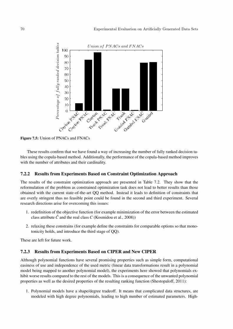
70 Experimental Evaluation on Artificially Generated Data Sets
PSfrag repla ements
Clayton PNACClayton FNACClaytonFrank PNACFrank FNAC FrankGumbel PNACGumbel FNACGumbelPer
centa
ge
offully
ranked
dec
isio
nta
bles Union of PNACs and FNACs
0102030405060708090100
Figure 7.5: Union of PNACs and FNACs
These results confirm that we have found a way of increasing the number of fully ranked decision ta-bles using the copula-based method. Additionally, the performance of the copula-based method improveswith the number of attributes and their cardinality.
7.2.2 Results from Experiments Based on Constraint Optimization Approach
The results of the constraint optimization approach are presented in Table 7.2. They show that thereformulation of the problem as constrained optimization task does not lead to better results than thoseobtained with the current state-of-the-art QQ method. Instead it leads to definition of constraints thatare overly stringent thus no feasible point could be found in the second and third experiment. Severalresearch directions arise for overcoming this issues:
1. redefinition of the objective function (for example minimization of the error between the estimatedclass attribute C and the real class C (Kosmidou et al., 2008))
2. relaxing these constrains (for example define the constraints for comparable options so that mono-tonicity holds, and introduce the third stage of QQ).
These are left for future work.
7.2.3 Results from Experiments Based on CIPER and New CIPER
Although polynomial functions have several promising properties such as simple form, computationaleasiness of use and independence of the used metric (linear data transformations result in a polynomialmodel being mapped to another polynomial model), the experiments here showed that polynomials ex-hibit worse results compared to the rest of the models. This is a consequence of the unwanted polynomialproperties as well as the desired properties of the resulting ranking function (Shestopaloff, 2011):
1. Polynomial models have a shape/degree tradeoff. It means that complicated data structures, aremodeled with high degree polynomials, leading to high number of estimated parameters. High-

Experimental Evaluation on Artificially Generated Data Sets 71
degree polynomial models are known for oscillatory behavior at the edges of the interval in whichthey are fitted, leading to poor interpolatory properties.
2. Additionally, when they provide good data fits, the goodness of fit may rapidly deteriorate outsidethe data range leading to poor extrapolatory properties.
3. Polynomial models have poor asymptotic properties. In comparison to copulas that use functionmapping [0,∞)→ [0,1], polynomials have an infinite response if some variable takes an infinitevalue.
4. The obtained coefficients in the polynomial models may be sensitive to small variations in the data.
5. Although many of the solutions here fulfill the monotonicity property required by the rankingfunction, polynomial models obtained with CIPER and New CIPER provide ties in the rankings inmost cases.
Details of the obtained results are given in Tables 6 and 7 in Appendix A.
7.2.4 Results Obtained with QQ when Modified with Impurity Functions
Although some of the linear methods exhibit the best results in comparison to the rest of the methods,linear methods have several drawbacks. Some of them are the following (Seeber and Lee, 2003):
1. Exhibit only linear relationships
Linear models tell how much a change in a variable effects the outcome variable leading to ameasurement of linear relationships between dependent and independent variables. However thismay not always be correct. A simple example is the relationship between income and age. In thisexample the relationship between two variables should be curved, since income tends to rise in theelderly parts of life, then to flatten and decline in retirement. One possible improvement may beachieved with fitting of piecewise linear functions (Greco et al., 2008), in which the independentvariable is partitioned into intervals and a separate linear function is fit to each interval. Still, thefollowing two drawbacks hold also for piecewise linear functions.
2. Provide a relationship only with the mean of the dependent variable
Linear regression provides a relationship between the mean of the dependent and independentvariables. However, the mean is not a complete description of a single variable. Consequently thelinear regression is not a complete description of relationships among variables. In order to dealwith this problem, one should use quantile regression, which is used with copulas in this thesis.
3. Variables must be independent
Linear regression assumes that the data at hand are independent, meaning that the attributes’values of one option have nothing to do with those of another. Although this situation is frequent,it is not always sensible. A typical example are student test scores when students come fromvarious classes, grades and schools. Students from the same class tend to be similar, thus theyare not independent. For example, such students would come from the same neighborhoods, theyhave the same teachers, etc. Unlike linear models, copulas exhibit different types of dependenciesexpressed via the values of θ , such as tail dependence and concordance.
According to the results of experiments, gP given with (4.5) provides best results in all three cases interms of monotonicity and full ranking. In spite of that, there are cases where copulas outperform them:

72 Experimental Evaluation on Artificially Generated Data Sets
1. The example provided in Table 7.3, consists of attributes and a class with different distributions.In this case the regression values obtained with the QQ and its modifications, represented with thecolumn Impurity 7.3, are the same and provide only partial ranking of options, as options 5 and 7are ranked the same.
2. The example provided in Table 7.4 consists of two symmetric attributes. There are six differentoptions, where one may argue that the methods should provide six different ranks. QQ basedmethods manage to provide five, while copulas provide six different ranks. The reasoning comesfrom the fact that the option 2, which receives the value of 2 for both attributes, is classified in thelest preferred class 1. This option differs from the rest two options in class 1 by having all vales ofits attributes other than 1, hence one could expect that it would receive different evaluation fromthe other two options.
Table 7.3: Example 1 of fully ranked options only with copula functions
No. A1 A2 C QQ Imp. Clayton ClaytonN Frank FrankN Gumbel GumbelN
1 1 1 1 1.0000 1.0000 1.0258 1.3473 1.2313 0.9213 1.2324 1.28952 2 1 2 1.7500 1.7500 2.2435 2.2907 2.1146 1.7335 1.9282 1.73623 3 2 2 2.2500 2.2500 3.4073 2.4508 3.9744 2.1642 3.9253 1.98654 1 3 2 2.0000 2.0000 1.6780 2.2129 1.5394 1.6003 1.7406 1.71275 3 1 3 2.9000 2.9000 2.8785 3.3582 3.5736 3.0142 3.4790 2.89206 1 2 3 2.7000 2.7000 1.4625 3.1707 1.3773 2.5774 1.4122 2.67777 2 2 3 2.9000 2.9000 2.7656 3.3433 2.3555 2.7719 2.1892 2.75838 2 3 3 3.1000 3.1000 3.0115 3.3758 2.6223 2.8250 2.6487 2.80599 3 3 3 3.3000 3.3000 3.6475 3.4600 4.4189 3.1823 4.6694 3.0155
Table 7.4: Example 2 of fully ranked options only with copula functions
No. A1 A2 C QQ Imp. Gumbel GumbelN Clayton ClaytonN Frank FrankN
1 3 1 1 1.0000 1.0000 1.7130 1.2515 0.7677 1.1514 1.6332 0.81022 2 2 1 1.0000 1.0000 1.9188 1.3895 2.0767 1.3928 1.8483 1.11753 1 3 1 1.0000 1.0000 1.7130 1.2515 0.7677 1.1514 1.6332 0.81024 2 1 2 2.0000 2.0000 1.6680 2.4587 0.7677 2.3244 1.5744 1.92325 1 2 2 2.0000 2.0000 1.6680 2.4587 0.7677 2.3244 1.5744 1.92326 1 1 3 2.6667 2.6667 1.5850 2.7087 0.7344 2.9848 1.4803 2.54547 3 2 3 3.1667 3.1667 2.0941 2.7941 2.1426 3.1793 2.0561 2.95178 2 3 3 3.1667 3.1667 2.0941 2.7941 2.1426 3.1793 2.0561 2.95179 3 3 3 3.3333 3.3333 2.4341 2.8511 3.3108 3.3408 2.4388 3.2218
7.2.5 Time Execution of Methods
One parameter which is of interest is the time needed to compute the different models and the outcomesfrom the regression functions. The results are given in Table 7.5 and are obtained by averaging the timeover 100 decision tables for all methods. The first and second columns in Table 7.5 give the number ofoptions and input attributes respectively. The third column provides the time that is needed to calculate

Experimental Evaluation on Artificially Generated Data Sets 73
all QQ based methods simultaneously, and the next three columns provide time needed to get results withthe copula-based method that uses Clayton, Frank and Gumbel copulas respectively, and the last columngives the execution time for constraint optimization method. All experiments are performed on UNIXbased system equipped with Intel(R) Core(TM) i7 CPU 870 @2.93GHz.
Table 7.5: Time execution in seconds of different methods averaged over 100 calculations
No. of options No. of inputs All QQ Clayton Frank Gumbel Constraint optimization
9 2 0.0349 0.3069 0.2883 0.2749 0.057527 3 0.1159 0.9934 0.6022 0.7718 1.428525 4 0.1017 1.8255 1.0135 0.8935 1.6216
It is clear that time execution is higher for the copula-based methods in comparison to other methodsand it increases with the number of input attributes. This can be explained with the fact that the number ofpossible FNAC structures increases with the number of input attributes, therefore the time for searchingthe solution increases as well.
7.3 Summary
The motivation of the presented experiments was to investigate the usage of different functions for eval-uation of options so that (2.3)–(2.5) are fulfilled. Presented results show that the usage of copulas isjustified by the number of possible solutions that they provide in each of the experiments. Based on thepresented results one may conclude the following.
• The best results in the first and the second experiment are obtained with the modified QQ methodwith the Gini population function.
• The best results in the third experiment are obtained using the combined copula-based results andQQ method modified with the Gini population.
• The combinations of copula-based results presented in Figure 7.5 show that combination of PNACsand FNACs improve the final evaluation of the copula-based regression method.
• Although the modified QQ with Gini population performs best, there are cases which may besolved only with the copula-based method, such the ones presented in Tables 7.3 and 7.4.

74 Experimental Evaluation on Artificially Generated Data Sets

75
8 Illustrative Examples
In this chapter, the copula-based approaches are illustrated on three examples. The examples illustrate themethodology on small decision tables, which consists of three to five attributes that receive values fromthe subset {1,2,3,4,5}. The examples were specially chosen to highlight several important properties ofcopula-based approach 1:
1. to show that monotonicity condition may be fulfilled when using FNAC for copula-based regres-sion, for cases when QQ fails to fulfill it,
2. to show that monotonicity condition may be fulfilled when using PNAC for copula-based regres-sion, for cases when QQ and FNACs fail to fulfill it, and
3. to demonstrate the behavior of copulas when dealing with symmetric decision tables
8.1 FNAC Solves the Breaching Monotonicity
The first example in this chapter demonstrates the ability of FNAC to produce regression functions whichovercome the problem of breaching monotonicity that is present when using QQ. The example that isconsidered for this purpose is given in Table 8.1. The first column is the option number and the nextfour columns are the quantitative values of attributes followed by the corresponding class. The last fourcolumns in Table 8.1 represent the calculations obtained with QQ, and with the different copula-basedregression functions from FNACs built with Clayton, Gumbel and Frank bi-variate copulas. The valuesof the θi parameters and the permutations of the attributes in the FNACs for each of the copula-basedmethods is given in Table 8.2. The values of the θi fulfill (5.16), thus each of the obtained regressionfunctions is considered as applicable for further examination.
In contrast to copula-based methods, QQ breaches the monotonicity in several occasions. For ex-ample, options 3 and 5 in Table 8.1, show that option 5 is better or at least as good as option 3 forall attributes. Consequently one would expect that the methods would rank option 5 better than option3. However, this is not the case with QQ calculations, which provide higher ranking value to option3. The same kind of behavior may be noticed with the following pairs of options: {(16,20), (17,20),(18,20),(19,20), (21,22), (21,24), (21,23), (21,25), (23,25), (24,25)}. Unlike QQ calculations, the valuesobtained with FNACs based on bi-variate copulas produce correct ranking which does not breach themonotonicity of the comparable options and provides full ranking of options. Hence this example showsthat this kind of failures of the QQ method that we want to address may be solved with the regressionfunctions obtained from FNACs.
1Methods that use modified QQ with impurity functions, polynomial functions and constraint optimization are also appliedon the three examples, and the results are given in Appendix B
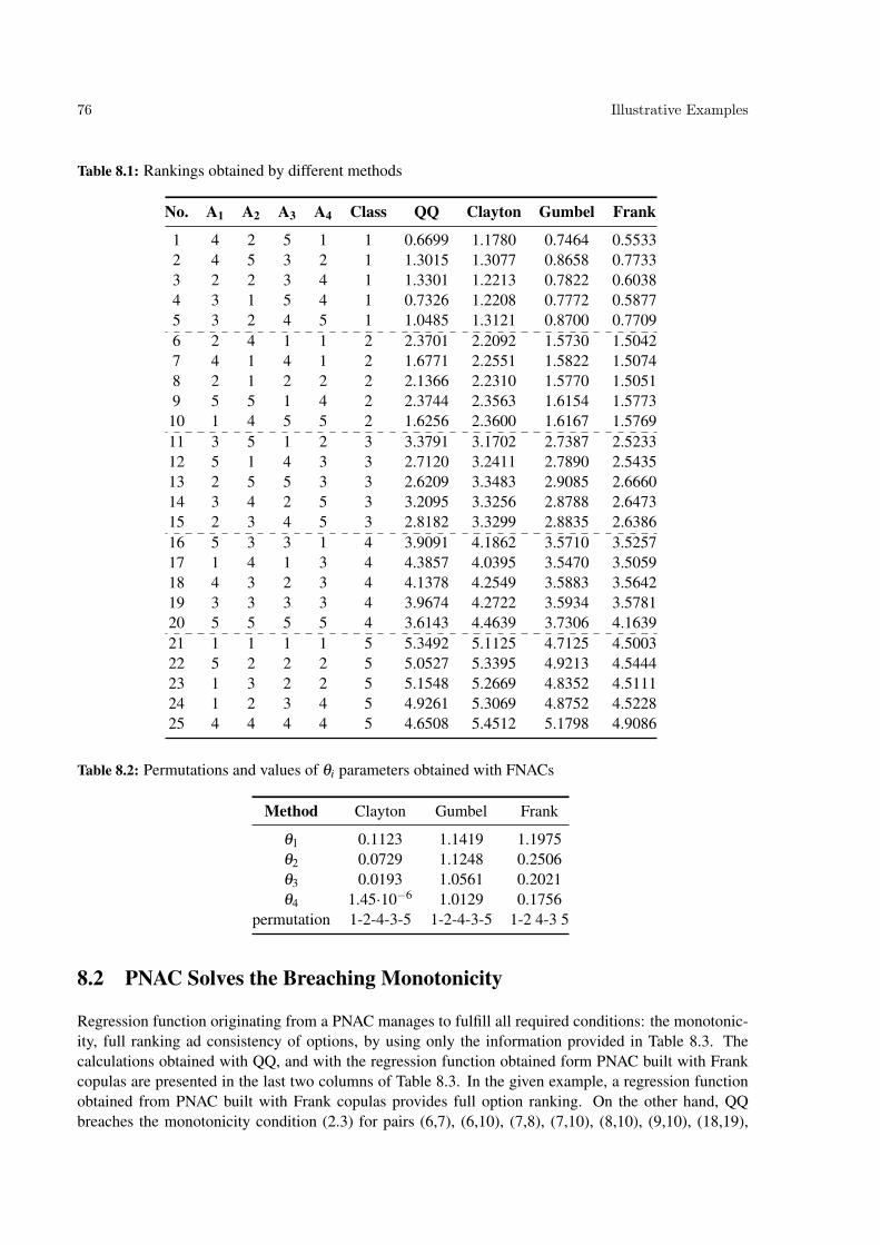
76 Illustrative Examples
Table 8.1: Rankings obtained by different methods
No. A1 A2 A3 A4 Class QQ Clayton Gumbel Frank
1 4 2 5 1 1 0.6699 1.1780 0.7464 0.55332 4 5 3 2 1 1.3015 1.3077 0.8658 0.77333 2 2 3 4 1 1.3301 1.2213 0.7822 0.60384 3 1 5 4 1 0.7326 1.2208 0.7772 0.58775 3 2 4 5 1 1.0485 1.3121 0.8700 0.77096 2 4 1 1 2 2.3701 2.2092 1.5730 1.50427 4 1 4 1 2 1.6771 2.2551 1.5822 1.50748 2 1 2 2 2 2.1366 2.2310 1.5770 1.50519 5 5 1 4 2 2.3744 2.3563 1.6154 1.577310 1 4 5 5 2 1.6256 2.3600 1.6167 1.576911 3 5 1 2 3 3.3791 3.1702 2.7387 2.523312 5 1 4 3 3 2.7120 3.2411 2.7890 2.543513 2 5 5 3 3 2.6209 3.3483 2.9085 2.666014 3 4 2 5 3 3.2095 3.3256 2.8788 2.647315 2 3 4 5 3 2.8182 3.3299 2.8835 2.638616 5 3 3 1 4 3.9091 4.1862 3.5710 3.525717 1 4 1 3 4 4.3857 4.0395 3.5470 3.505918 4 3 2 3 4 4.1378 4.2549 3.5883 3.564219 3 3 3 3 4 3.9674 4.2722 3.5934 3.578120 5 5 5 5 4 3.6143 4.4639 3.7306 4.163921 1 1 1 1 5 5.3492 5.1125 4.7125 4.500322 5 2 2 2 5 5.0527 5.3395 4.9213 4.544423 1 3 2 2 5 5.1548 5.2669 4.8352 4.511124 1 2 3 4 5 4.9261 5.3069 4.8752 4.522825 4 4 4 4 5 4.6508 5.4512 5.1798 4.9086
Table 8.2: Permutations and values of θi parameters obtained with FNACs
Method Clayton Gumbel Frank
θ1 0.1123 1.1419 1.1975θ2 0.0729 1.1248 0.2506θ3 0.0193 1.0561 0.2021θ4 1.45·10−6 1.0129 0.1756
permutation 1-2-4-3-5 1-2-4-3-5 1-2 4-3 5
8.2 PNAC Solves the Breaching Monotonicity
Regression function originating from a PNAC manages to fulfill all required conditions: the monotonic-ity, full ranking ad consistency of options, by using only the information provided in Table 8.3. Thecalculations obtained with QQ, and with the regression function obtained form PNAC built with Frankcopulas are presented in the last two columns of Table 8.3. In the given example, a regression functionobtained from PNAC built with Frank copulas provides full option ranking. On the other hand, QQbreaches the monotonicity condition (2.3) for pairs (6,7), (6,10), (7,8), (7,10), (8,10), (9,10), (18,19),

Illustrative Examples 77
Table 8.3: Rankings obtained with QQ and Frank copula using the PNAC given in Figure 5.7a, beforeand after applying equations (3.3)–(3.5)
No. A1 A2 A3 A4 Class QQ Frank PNAC
1 2 4 1 1 1 1.3663 1.26502 5 2 2 2 1 0.8669 0.74093 5 1 4 3 1 0.6337 0.73134 2 2 3 4 1 0.9060 1.07775 3 1 5 4 1 0.6702 1.02136 4 2 5 1 2 1.9640 1.64997 2 1 2 2 2 2.1754 1.57108 4 4 4 4 2 1.9802 2.14479 1 4 5 5 2 2.2128 2.298410 5 5 5 5 2 1.7872 2.386711 4 3 2 3 3 3.1848 2.723212 3 3 3 3 3 3.2488 2.853613 3 4 2 5 3 3.2262 3.102314 3 2 4 5 3 2.7512 2.908215 2 3 4 5 3 3.0527 3.210616 5 3 3 1 4 3.8831 3.822917 4 1 4 1 4 3.6848 3.579418 1 4 1 3 4 4.3152 4.011719 2 5 5 3 4 4.1305 4.378420 5 5 1 4 4 3.9456 4.140521 1 1 1 1 5 5.0429 4.573822 3 5 1 2 5 5.2787 5.256323 1 3 2 2 5 5.1599 4.962924 4 5 3 2 5 5.0352 5.352625 1 2 3 4 5 4.7213 4.9564
(18,20), (21,24), (21,25), (22,24), (23,24).As a lesson from the last two examples, it is recommend to build PNAC in cases when regression
functions obtained from FNAC fail to provide full ranking of options. The background for this rec-ommendation comes from the fact that when working with copulas, it is less complex to calculate theregression functions obtained with FNAC than with PNAC.

78 Illustrative Examples
8.3 Evaluation of Symmetric Decision Tables
Options in symmetric decision tables are evaluated with one-parametric copulas as explained in sec-tion 5.4.1. One such example is given in Table 8.4. It is taken from a real case example, which is furtherdiscussed in section 9.2. In this example, the qualitative values of attributes A–D are converted into quan-titative one so that they form a monotone decision table, represented with columns A1–D1. Symmetricare the attributes A and B.
Table 8.4: Utility function (A–D) and mapping from the qualitative attributes into quantitative ones (A1–D1). Basic attributes are: A–Generality, B–Scalability and C–NoiseSensitivity. The aggregated attributeis D–Robustness.
No A B C D A1 B1 C1 D1
1 ’low’ ’low’ ’high’ ’very low 1 1 1 12 ’med’ ’low’ ’high’ ’low’ 2 1 1 23 ’high’ ’low’ ’high’ ’low’ 3 1 1 24 ’low’ ’med’ ’high’ ’low’ 1 2 1 25 ’med’ ’med’ ’high’ ’low’ 2 2 1 26 ’low’ ’high’ ’high’ ’low’ 1 3 1 27 ’low’ ’low’ ’med’ ’low’ 1 1 2 28 ’med’ ’low’ ’med’ ’low’ 2 1 2 29 ’low’ ’med’ ’med’ ’low’ 1 2 2 210 ’low’ ’low’ ’low’ ’low’ 1 1 3 211 ’high’ ’med’ ’high’ ’med’ 3 2 1 312 ’med’ ’high’ ’high’ ’med’ 2 3 1 313 ’high’ ’high’ ’high’ ’med’ 3 3 1 314 ’high’ ’low’ ’med’ ’med’ 3 1 2 315 ’med’ ’med’ ’med’ ’med’ 2 2 2 316 ’high’ ’med’ ’med’ ’med’ 3 2 2 317 ’low’ ’high’ ’med’ ’med’ 1 3 2 318 ’med’ ’high’ ’med’ ’med’ 2 3 2 319 ’med’ ’low’ ’low’ ’med’ 2 1 3 320 ’high’ ’low’ ’low’ ’med’ 3 1 3 321 ’low’ ’med’ ’low’ ’med’ 1 2 3 322 ’med’ ’med’ ’low’ ’med’ 2 2 3 323 ’low’ ’high’ ’low’ ’med’ 1 3 3 324 ’high’ ’high’ ’med’ ’high’ 3 3 2 425 ’high’ ’med’ ’low’ ’high’ 3 2 3 426 ’med’ ’high’ ’low’ ’high’ 2 3 3 427 ’high’ ’high’ ’low’ ’very high’ 3 3 3 5
Here QQ method and its modifications that use impurity functions (4.4)–(4.6) provide equal weightvalues wi for each of the attributes in (3.2). Hence these cases represent an intersection of the QQmethods because all of them provide the same option evaluation. Evaluations and option ranks using QQmethod are given in the column QQ in Table 8.5 and Table 8.6 respectively.
Table 8.6 shows that QQ (as well as its modifications with impurity functions) divide the options into7 different ranks, Clayton divides them in 8 and Frank and Gumbel provide 10 different ranks. CIPERmanages to distinguish seven ranks, while New CIPER finds a polynomial structure that distinguishes

Illustrative Examples 79
among all 27 options. The question that has to be answered is which ranking one should consider asthe most acceptable? In other words, which information in the decision table one may use in order todistinguish among the different rankings?
Firstly, in cases of symmetric attributes, an acceptable aggregation function is the one which providesthe same ranking for the symmetric attributes. Therefore the condition for full ranking given with (2.4)has to be relaxed for symmetric attributes. Consequently, the ranking obtained with New CIPER is notacceptable. Considering the heuristics based on which New CIPER works, and relaxing it to work forsymmetric attributes, leads to the results obtained with CIPER. The ranking with CIPER are the same asthe ranking obtained with QQ.
Table 8.5: Option evaluation using QQ method and Clayton, Frank and Gumbel copulas
No. A1 B1 C1 D1 QQ Clayton ClaytonN Gumbel GumbelN Frank FrankN
1 1 1 1 1 1.0000 1.6598 1.0000 2.1738 0.5898 2.3049 1.47732 2 1 1 2 1.8750 1.6610 0.8865 2.1955 1.5657 2.3229 2.18573 3 1 1 2 2.1250 1.6610 0.8865 2.2077 1.5868 2.3325 2.19384 1 2 1 2 1.8750 1.6610 0.8865 2.1955 1.5657 2.3229 2.18575 2 2 1 2 2.1250 1.6631 0.8886 2.2483 1.6569 2.3655 2.22146 1 3 1 2 2.1250 1.6610 0.8865 2.2077 1.5868 2.3325 2.19387 1 1 2 2 1.8750 1.6610 0.8865 2.1955 1.5657 2.3229 2.18578 2 1 2 2 2.1250 1.6631 0.8886 2.2483 1.6569 2.3655 2.22149 1 2 2 2 2.1250 1.6631 0.8886 2.2483 1.6569 2.3655 2.221410 1 1 3 2 2.1250 1.6610 0.8865 2.2077 1.5868 2.3325 2.193811 3 2 1 3 2.8750 1.6631 2.3494 2.2793 2.6020 2.3900 2.635312 2 3 1 3 2.8750 1.6631 2.3494 2.2793 2.6020 2.3900 2.635313 3 3 1 3 3.1250 1.6631 2.3494 2.3224 2.6381 2.4241 2.641814 3 1 2 3 2.8750 1.6631 2.3494 2.2793 2.6020 2.3900 2.635315 2 2 2 3 2.8750 2.7437 2.6219 2.3896 2.6943 2.4821 2.652916 3 2 2 3 3.1250 2.7461 2.6225 2.4832 2.7727 2.5591 2.667617 1 3 2 3 2.8750 1.6631 2.3494 2.2793 2.6020 2.3900 2.635318 2 3 2 3 3.1250 2.7461 2.6225 2.4832 2.7727 2.5591 2.667619 2 1 3 3 2.8750 1.6631 2.3494 2.2793 2.6020 2.3900 2.635320 3 1 3 3 3.1250 1.6631 2.3494 2.3224 2.6381 2.4241 2.641821 1 2 3 3 2.8750 1.6631 2.3494 2.2793 2.6020 2.3900 2.635322 2 2 3 3 3.1250 2.7461 2.6225 2.4832 2.7727 2.5591 2.667623 1 3 3 3 3.1250 1.6631 2.3494 2.3224 2.6381 2.4241 2.641824 3 3 2 4 4.0000 2.7500 3.6229 2.6311 3.6854 2.6814 3.551925 3 2 3 4 4.0000 2.7500 3.6229 2.6311 3.6854 2.6814 3.551926 2 3 3 4 4.0000 2.7500 3.6229 2.6311 3.6854 2.6814 3.551927 3 3 3 5 5.0000 3.8617 4.7091 2.8956 4.7587 2.9035 4.5487
The number of different options that are not symmetric among themselves, in Table 8.6 is 10. There-fore one may argue that methods that provide 10 different ranks are better than those that provide lessranks, under the assumption that monotonicity and consistency are fulfilled in both cases. To support thisargument for the particular example, one has to consider the rank of the options according to the classesattribute. It classifies the options from 1 to 5, with preference order given with 1≺ 2≺ 3≺ 4≺ 5 . Can

80 Illustrative Examples
Table 8.6: Ranks of options using QQ and FNACs based on Clayton, Frank and Gumbel bi-variate copula
No. A1 B1 C1 D1 QQ Clayton Gumbel Frank1 1 1 1 1 1 1 1 12 2 1 1 2 2 2 2 23 3 1 1 2 3 3 3 34 1 2 1 2 2 2 2 25 2 2 1 2 3 4 4 46 1 3 1 2 3 3 3 37 1 1 2 2 2 2 2 28 2 1 2 2 3 4 4 49 1 2 2 2 3 4 4 410 1 1 3 2 3 3 3 311 3 2 1 3 4 5 5 512 2 3 1 3 4 5 5 513 3 3 1 3 5 5 6 614 3 1 2 3 4 5 5 515 2 2 2 3 4 6 7 716 3 2 2 3 5 7 8 817 1 3 2 3 4 5 5 518 2 3 2 3 5 7 8 819 2 1 3 3 4 5 5 520 3 1 3 3 5 5 6 621 1 2 3 3 4 5 5 522 2 2 3 3 5 7 8 823 1 3 3 3 5 5 6 624 3 3 2 4 6 8 9 925 3 2 3 4 6 8 9 926 2 3 3 4 6 8 9 927 3 3 3 5 7 9 10 10
this information somehow lead to further separations of option ranks from 7 to 10?One may notice that the only option that belongs to class 1 has evaluation of all attributes as 1.
Options belonging to class 2 have one or two attributes that are evaluated with 1. Options that belong toclass 3 have one or none of the attributes evaluated with 1, while none of the options in classes 4 and 5have evaluation of attributes equal to one. One may conclude that more preferred options are the oneswith less evaluation of attributes to one. This information is incorporated in Clayton, Frank and Gumbelcopulas, and hence it leads to three more ranks than QQ and CIPER methods.

81
9 Applications of Copula-Based Method for Option Ranking
This chapter demonstrates the applicability of the copula-based regression method for option ranking onhierarchically combined decision tables which are characteristic decision problems with larger numberof attributes, usually more than five. In the following two sections two examples are provided showinghow and when the copula-based regression for option ranking in hierarchical settings may be used. In thefirst example the copula-based decision support system (DSS) is used for assessment of 840 electricallycommutated (EC) motors (Mileva-Boshkoska et al., 2013). In the second example a model for rankingof workflows that are uploaded by researchers on the website www.myexperiment.org is built (Mileva-Boshkoska et al., 2012).
9.1 Assessment of Electrically Commutated Motors
Quality assessment of finished products (QAFP) is usually the final step in a manufacturing line. It isperformed by aggregating feature set values according to a set of pre-defined preferences and rules. Sucha task can be implemented by applying concepts of decision support systems (DSS).
A typical structure of QAFP system is shown in Figure 9.1. Such a system has two inputs: features,extracted from the performed measurements, and expert’s preferences regarding the final quality eval-uation. These inputs are processed through the two main stages: integration of system’s features andexpert’s preferences, and definition of a copula-based DSS for assessment of overall quality and rankingof finished products. Implementation of these steps has to ensure high sensitivity to the variations in thequality of the finished product. Consequently, each segment of the system has to be custom-made for theproblem in hand.
The input of the system is a set of measured features calculated from the acquired vibrations gener-ated by the examined electronically commutated (EC) motor. Furthermore, the system employs availableexpert’s knowledge provided in DEX model tree. Employing copula-based regression functions resultedin a full quality ranking of EC motors. The system was evaluated on a batch of 840 motors. Due to thedifferent background of each segment of this problem, each one is described in details in a depth that isrequired to understand the problem at hand.
Figure 9.1: Structure of the end-quality assessment system

82 Applications of Copula-Based Method for Option Ranking
The extracted feature set should contain the most useful features for determining the fault conditionof the monitored system (Vachtsevanos et al., 2006). In absence of faults, feature values should belongto the set of nominal (admissible) values. Any discrepancy in one or several features is regarded as apresence of fault, hence indicating decrease in the overall quality. In order to meet such requirements,two steps should be performed: the most informative features should be selected based on existing faultmodels, and extraction of their values should be performed using fast and accurate signal processingtechniques.
The problem of specifying the most informative feature set in the case of electrical motors has beenaddressed by many authors (Boškoski et al., 2011; Didier et al., 2007; Juricic et al., 2001; Röpke andFilbert, 1994; Sasi et al., 2001). Generally features are extracted from vibration and/or electrical signals.In our particular case, the features were extracted solely from vibration signals. From a plethora ofavailable signal processing methods, we opted for the well established approach using envelope analysis(Jardine et al., 2006; Peng and Chu, 2004; Randall and Antoni, 2011; Sawalhi et al., 2007). As a pre-processing step we used spectral kurtosis (Antoni, 2006) and cyclostationary analysis (Boškoski et al.,2010), due to their capabilities of selecting the most appropriate frequency band for envelope analysis,hence significantly improving the sensitivity of the approach.
The construction of the copula-based DSS starts with integration of features with expert’s prefer-ences. The integration addresses the issues of fusing information from the extracted features into anabstract quality rank based on a set of pre-defined expert’s preferences. Usually these preferences areexpressed using qualitative grades. For this purpose, qualitative aggregation functions are suitable can-didates, such as the ones proposed in the DEX methodology. As DEX uses qualitatively describedaggregation functions, it leads to partial ranking of the options at hand. To achieve a full ranking ofoptions, we employ copula functions. Unlike linear regression functions, which tend to provide partialranking when two or more attributes receive the same weight value (Mileva-Boshkoska and Bohanec,2011) or evidential reasoning method which sometimes leads to evaluations that are not in line with theexpert’s expectations (Boškoski et al., 2011), the usage of DEX and copula-based regression leads tohigh sensitivity to small variations of the input values. This process produces twofold output informa-tion. Firstly, the constructed copula-based DSS yields a grade (also called class) to which the examinedEC motor belongs. Secondly, it produces a rank value that can be employed for ordering the EC motorswithin each grade. Therefore, one can easily specify the position of each finished EC motor within thepopulation of produced units based on its quality rank.
Implementing quality assessment systems has the potential for creating sustainable competitive ad-vantage (Reed et al., 2000). The proposed quality assessment system allows immediate detection ofquality change for each produced item individually. Furthermore, the quality assessment output can beused by any subsequent manufacturing execution system, which will handle any general changes in theproduction quality (Ertugrul and Aytac, 2009; Orth et al., 2012).
9.1.1 Feature Selection and Organization in DEX Structure
According to several surveys, bearing faults represent the most common cause for failure of mechanicaldrives (Albrecht et al., 1986; Crabtree, 2010). Besides bearing faults, in the context of EC motors, rotorfaults are also frequent. Therefore we propose a feature set that describes these two groups of faults.
Proper selection of the feature set is crucial for the overall effectiveness of the quality assessment.When analyzing vibration signals generated under constant operating conditions, feature values are usu-ally the amplitudes of particular spectral components.
Rotor faults Due to improper manufacturing or improper assembly, rotor faults include:
• mass unbalance, and

Applications of Copula-Based Method for Option Ranking 83
• misalignment faults.
The presence of either of the faults influences the mass displacement on the rotor, hence changing itsmoment of inertia. Under constant rotational speed, such a change can be detected by analysing thegenerated vibrations and it is generally expressed as an increase of the amplitudes of the spectral compo-nents at the rotational frequency frot and its higher harmonics n× frot , n∈ {2,3, · · ·} (Xu and Marangoni,1994).
Bearing faults Bearings in EC motors are the most susceptible element to mechanical faults. Duringthe manufacturing process the most common causes for introducing bearing faults are improper bear-ing lubrication, improper mounting and alignment, as well as improper handling during the assemblyprocess.
The detection of these faults is a challenging task. Vibrations, caused by a bearing fault, originatefrom impacts produced by the rolling elements hitting a damaged place. Each time a hit occurs, an exci-tation of system eigenmodes occurs in terms of an impulse response s(t). The frequency of occurrenceof these impulse responses can be estimated using the rotational speed frot of the rotating ring and thephysical characteristics of the bearing, i.e. the pitch diameter D, the rolling element diameter d, thenumber of rolling elements Z, and the contact angle α (see Figure 9.2). Using these parameters thebearing fault frequencies can be calculated according to the relations shown in Table 9.1 (Tandon andChoudhury, 1999).
D
d
PitchDiameter
Ball Diameter
Contact angle
Outer racefault
Inner racefault
Rolling elementfault
Figure 9.2: Bearing dimensions used for the calculation of the bearing’s characteristic frequencies
Table 9.1: Bearing frequencies (Tandon and Choudhury, 1999)
Name Relation to the rotational frequencyfrot
Bearing pass frequency inner race(BPFI)
fBPFI =Z frot
2
(1+ d
D cosα)
Bearing pass frequency outer race(BPFO)
fBPFO = Z frot2
(1− d
D cosα)
Fundamental train frequency (FTF) fFT F = frot2
(1− d
D cosα)
Ball spin frequency (BSF) fBSF = D frot2d
(1−( d
D cosα)2)

84 Applications of Copula-Based Method for Option Ranking
Figure 9.3: From qualitative attributes and quantitative features to final quantitative evaluation
9.1.2 Implementation Within the Quality Assessment System
The implementation of the copula-based quality assessment system follows the steps shown in Figure 9.3.Firstly, one has to present the decision maker’s preferences in a qualitative decision table. Then, a map-ping from qualitative attributes into quantitative ones has to be performed. Finally, for each quantitativedecision table, a copula function is defined. After the completion of these steps, one can apply theAlgorithms 6 and 7 for copula-based regression described in section 6.6.
DEX Hierarchical Model
Assessing the overall motor quality rank directly from the measured features is a rather difficult task.Therefore, the problem is transformed into a hierarchical decision making model in which the overallmechanical quality rank is obtained by aggregating two simpler attributes: rotor quality and bearingsquality as shown in Table 9.2. The former attribute can be directly assessed from the measured featuresdescribed in subsection 9.1.1. The latter attribute is still complex as it can be further decomposed intofour simpler attributes: inner ring quality, outer ring quality, quality of the rolling elements and qualityof the bearing cage. These four attributes can be assessed from the measured features describing bearingcondition, as shown in section 9.1.1. Based on this logical structure a DEX hierarchical model is built,which is shown in the first column of Table 9.2, where the aggregated attributes are given with uppercases and the basic attributes are given in plain letters.
Following the expert’s preferences and knowledge, each attribute in the proposed hierarchical struc-ture was described or aggregated using the expert’s defined scale with five qualitative values:
QC = {not satis f actory,good,very good,excellent, top}.
For instance, the aggregation of the basic attributes BPFI and 2×BPFI into attribute Inner ring is givenin the first three columns of Table 9.3. These aggregations may be interpreted as a set of if-then rules,for instance, the last row in Table 9.3 can be interpreted as follows:
if BPFI is Top and 2× BPFI is Top thenInner ring is Top
end if.

Applications of Copula-Based Method for Option Ranking 85
Table 9.2: DEX model tree and qualitative and quantitative evaluations of EC motors 744 and 9
Attribute Evaluation of motor 744 Evaluation of motor 9Qualitative Quantitative Qualitative Quantitative
MECHANICAL QUALITYROTOR QUALITY
frot
2× frot
VarianceBEARINGS QUALITY
INNER RINGBpfi2×Bpfi
OUTER RINGBpfo2×Bpfo
ROLL ELEMENTSBsf2×Bsf
Ftf
not satisfactorytoptoptoptopnot satisfactorygoodgoodvery goodgoodgoodvery goodnot satisfactorynot satisfactoryvery goodgood
1.33894.97024.7851550.75921.95831.70962.63191.80091.90432.16600.88101.23962.61002.6279
very goodtoptoptoptopgoodvery goodvery goodexcellentgoodvery goodgoodvery goodvery goodexcellentvery good
3.30565.03025551.78992.80512.82272.88302.18893.02032.02382.84542.93612.92883.0974
9.1.3 Qualitative to Quantitative Value Mapping
After defining the qualitative model, the next step is to obtain the quantitative model. For that reason,each of the qualitatively defined expert rules and preference values are mapped into a quantitative one.In the qualitative model, the preferences given by the decision maker are:
not satis f .≺ good ≺ very good ≺ excellent ≺ top
where the sign ≺ stands for “is strictly less preferred than”. In the quantitative model, these values aremapped into {1, 2, 3, 4, 5} respectively. In addition, the sign ≺ is mapped into <, where < stands for ‘isgreater than’. The mapping ensures that the more preferred values are mapped into greater numbers. Anexample of the mapping is given in the last three columns of Table 9.7, where the qualitative values ofattributes Bpfi, 2× Bpfi and Inner ring are mapped into quantitative values of A1, A2 and C respectively.
Based on the QQ model given in Table 9.2, six linear aggregation functions are built for each of theaggregated attributes. Each aggregation function is built from the quantitative decision table, such as theone given with the last three columns in Table 9.3. The aggregation functions are obtained by applying(3.1)–(3.5). For the given example in Table 9.3, function g in (3.1) reads:
g = 0.5600A1 +0.5600A2−0.9200. (9.1)
After applying (3.4)–(3.5) on (9.1) we obtain:
fc =
0.2976g+0.6071, if c = 1
0.5952g+1.0476, if c = 2
0.5952g+1.3810, if c = 3
0.5952g+1.7143, if c = 4
0.8929g+0.8214, if c = 5.

86 Applications of Copula-Based Method for Option Ranking
Here fc is an estimation of C in Table 9.3. The obtained quantitative value fc for the attribute Inner ringis then propagated to the aggregation function in the next level, which estimates the quantitative valueof Bearings quality. This procedure is repeated until the final evaluation of the Mechanical Quality isachieved.
Table 9.3: Expert defined rules for aggregation of the attribute Inner ring and mapping from the qualita-tive attribute values into quantitative ones.
BPFI 2xBPFI Inner ring A1 A2 C
‘not satisf.’ ‘not satisf.’ ‘not satisf.’ 1 1 1‘not satisf.’ ‘good’ ‘not satisf.’ 2 1 1‘not satisf.’ ‘very good’ ‘not satisf.’ 1 3 1‘not satisf.’ ‘excellent’ ‘not satisf.’ 1 4 1‘not satisf.’ ‘top’ ‘not satisf.’ 1 5 1
‘good’ ‘not satisf.’ ‘not satisf.’ 2 1 1‘good’ ‘good’ ‘good’ 2 2 2‘good’ ‘very good’ ‘good’ 2 3 2‘good’ ‘excellent’ ‘very good’ 2 4 3‘good’ ‘top’ ‘very good’ 2 5 3
‘very good’ ‘not satisf.’ ‘not satisf.’ 3 1 1‘very good’ ‘good’ ‘good’ 3 2 2‘very good’ ‘very good’ ‘very good’ 3 3 3‘very good’ ‘excellent’ ‘very good’ 3 4 3‘very good’ ‘top’ ‘excellent’ 3 5 4‘excellent’ ‘not satisf.’ ‘not satisf.’ 4 1 1‘excellent’ ‘good’ ‘very good’ 4 2 3‘excellent’ ‘very good’ ‘very good’ 4 3 3‘excellent’ ‘excellent’ ‘excellent’ 4 4 4‘excellent’ ‘top’ ‘excellent’ 4 5 4
‘top’ ‘not satisf.’ ‘not satisf.’ 5 1 1‘top’ ‘good’ ‘very good’ 5 2 3‘top’ ‘very good’ ‘excellent’ 5 3 4‘top’ ‘excellent’ ‘excellent’ 5 4 4‘top’ ‘top’ ‘top’ 5 5 5
9.1.4 Integration of Feature Values and Expert’s Preferences
Experts’ preferences may be subjective, even inconsistent, and may differ between experts. Therefore inthe development of this model we paid special attention to the consistency of the evaluation model. First,whenever possible, we closely followed the ISO 10816 standard, which denotes the maximal allowedvibrations for particular drives. Second, additional requirements were specified by the manufactureritself as well as the targeted customers. Finally, the DEX model was built which is guaranteed to becomplete and consistent.
The actual integration of the measured feature values and the expert’s preferences is performed usingfuzzification. The expert’s preference is towards motors with lower vibrations, hence lower featurevalues are more preferred. The maximum allowed value for each feature determines the limit for the notsatisfactory grade. This limit was determined either by governing standard rules or by the company’s

Applications of Copula-Based Method for Option Ranking 87
not satisfactory [feature units]excellent
very good goodtop
1
0
[deg
ree
of
mem
ber
ship
]
Figure 9.4: Intervals for mapping feature values to quantitative ones
Figure 9.5: FNAC structure for aggregation of the attribute Inner Ring
quality requirements. The remaining interval below the limit for the not satisfactory grade was divideddyadically, as shown in Figure 9.4. Such mapping ensures more sensitivity at lower feature values. Thefeature values fi are fuzzified and mapped accordingly into the expert’s defined interval [1,5], employingthe relation:
Ai( fi) = ∑n
µn( fi)cn. (9.2)
Here µn( fi) is the membership function of the nth rule as given in Figure 9.4, and cn ∈ {1,2,3,4,5} arevalues of the class attribute.
9.1.5 Constructing the Copula-Based Regression Functions
According to the model shown in Table 9.2 there are six aggregation tables. For each of the decisiontables, there are two possibilities: to build FNACs or one-parametric copulas. Both approaches are givenin continuation.
Constructing FNACs
For each decision table, a FNAC based on the Frank bi-variate copula was built. Hence six copula-basedregression functions were derived. The obtained values from (9.2) enter the appropriate copula-basedregression functions, and for each of them a copula-based regression value is calculated. For the givenexample in Table 9.3, we built a FNAC, such as the one given in Figure 9.5. When building the FNAC,the attributes enter the input level at any position as long as the obtained FNAC fulfills (5.16). For theattribute Inner Ring, in the obtained FNAC, first the attribute BPFI is coupled with the output Inner ringforming a copula Cθ1 with parameter θ1 = 5.5. The obtained copula is then coupled with the attribute

88 Applications of Copula-Based Method for Option Ranking
2×BPFI leading to the copula Cθ2 with parameter θ2 = 2.5529. The values of θ1 and θ2 fulfill (5.16)thus, we may proceed with the regression procedure. Here, the position of the dependent variable Innerring is p = 2 hence we use Algorithm 7 for regression.
The regression part is solved as an iterative procedure starting from the highest level of FNAC anddescending down to the level which contains the dependent variable by substituting the correct quantitiesfor q in the Frank regression equation (see last column in Table 5.1). In each of the iterations, the valueof q is substituted with a vector of regression values obtained from the previous iteration procedure. Forexample, in the first iteration the value of v3 is obtained using Frank-based regression equation given inTable 5.1 that leads to:
v3 =1
2.5529log
−e2.5529(1−0.5+0.5e2.5529u3)
−e2.5529 +0.5e2.5529−0.5e2.5529u3. (9.3)
The values obtained with (9.3) are propagated to the next iteration, the last one, that provides the finalcopula regression equation v:
v =1
5.5log−e5.5(1− v3 + v3e5.5u1)
−e5.5 + v3e5.5− v3e5.5u1.
The regression values v are afterwards normalized in order to retain consistency with the qualitativemodel as defined in (3.4)–(3.5) (Stage 3 in Figure 3.2):
fc =
0.2667F−1(v)+0.4752, if c = 1
0.5564F−1(v)+1.0214, if c = 2
0.3659F−1(v)+1.9901, if c = 3
0.4639F−1(v)+2.3345, if c = 4
1.0834F−1(v)+0.1608, if c = 5.
(9.4)
The obtained values from (9.4) are propagated in the higher hierarchical level, where they are used asinputs in the next regression function. The procedure is recursively repeated up to the topmost decisiontable. The result of the topmost decision table is regarded as the overall quality rank for each motor.
Constructing One-Parametric Copulas
In this approach, for each decision table, a one-parametric Clayton multi-variate copula was built. Hencesix copula-based regression functions were derived. For each copula, only one parameter θ is obtained.For example, for the attribute Mechanical quality, the copula has parameter θ1 = 0.2953.
The regression is performed in one step by using the regression equation for the Clayton copula givenin Table 5.1:
v = (1−u−0.2953 +(0.5u1.2953)−0.29531.2953 )−
10.2953 .
In the last equation, the values of u are obtained by building one-parametric copula with θ1 = 0.2953with all input attributes. This is possible due to the associative property of the Archimedean copulas:C(C(u1,u2),u3) =C(u1,C(u2,u3)). The regression values v are afterwards normalized in order to retainconsistency with the qualitative model as defined in (3.4)–(3.5) (Stage 3 in Figure 3.2):
fc =
0.2801F−1(v)+0.9049, if c = 1
1.6325F−1(v)−1.1857, if c = 2
1.8293F−1(v)−1.1183, if c = 3
2.7279F−1(v)−2.9315, if c = 4
5.7322F−1(v)−10.6250, if c = 5.

Applications of Copula-Based Method for Option Ranking 89
9.1.6 The Final Evaluation of EC Motors and Two Characteristic Examples
The Assessment Rig
Each EC motor is tested using the assessment rig shown in Figure 9.6. The rig consists of a fixed pedestalon top of which a metal disk is positioned. The metal disk holds three rubber dampers that suspend thetested EC motor. The experiment starts by positioning the EC motor vertically on the rubber dampers insuch a way that the drive-end bearing is on the bottom. Afterwards, two accelerometers are positionedon the motor housing nearest to the both bearings. The test-rig minimizes the environmental influence,hence guaranteeing sufficiently constant experimental conditions.
The data acquisition process commences as soon as the nominal rotational speed is reached. Firstly,both vibration signals are low-pass filtered with cut-off frequency at 22 kHz. Afterwards, both signalsare sampled at 60 kHz. During the whole data acquisition process the nominal rotational speed of frot =38 Hz is maintained. Each acquisition process lasts 8 seconds. After finishing the acquisition the motoris decelerated down to the stop position.
Electrical
Motor
Power
Supply
Vibration
sensorsSignal
conditioning unit
Figure 9.6: The prototype assessment point
Results on a Test Batch of Motors
During the evaluation process a test batch of 840 EC motors was analyzed. The overall quality rankis shown in Figure 9.7. For the purpose of testing the system on small differences in data, during theinitial start-up of the line, motors with intentionally introduced various mechanical faults were evaluated.Consequently, there are many motors with different overall quality rank.
From the results shown in Figures 9.7 and 9.8, it is clearly visible that the quality ranks of the testedmotors are spread over the interval [0.5,5.5]. This is an indication that the proposed copula-based DSS ishighly sensitive even to minor variations in the motor quality. Unlike methods that use weighted utilityfunctions, where options with not satisfactory feature values are ranked highly, this approach averts suchperformance. Such example is given in (Boškoski et al., 2011), where the first 130 motors were evaluatedusing evidential reasoning approach which lead to cases where final evaluations were inconsistent withthe expert’s preferences. Besides the overall quantitative evaluation, the calculated rank also shows theclass of each EC motor.
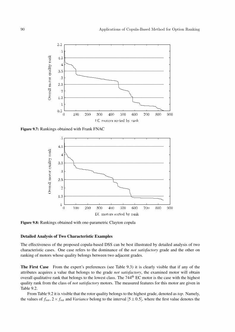
90 Applications of Copula-Based Method for Option Ranking
PSfrag repla ements
EC motors sorted by rankOverallmotorqualityrank
0 100 200 300 400 500 600 700 800 9000.511.522.533.544.555.5
Figure 9.7: Rankings obtained with Frank FNACPSfrag repla ements
EC motors sorted by rankOverallmotorqualityrank
0 100 200 300 400 500 600 700 800 90011.522.533.544.55
Figure 9.8: Rankings obtained with one-parametric Clayton copula
Detailed Analysis of Two Characteristic Examples
The effectiveness of the proposed copula-based DSS can be best illustrated by detailed analysis of twocharacteristic cases. One case refers to the dominance of the not satisfactory grade and the other onranking of motors whose quality belongs between two adjacent grades.
The First Case From the expert’s preferences (see Table 9.3) it is clearly visible that if any of theattributes acquires a value that belongs to the grade not satisfactory, the examined motor will obtainoverall qualitative rank that belongs to the lowest class. The 744th EC motor is the case with the highestquality rank from the class of not satisfactory motors. The measured features for this motor are given inTable 9.2.
From Table 9.2 it is visible that the rotor quality belongs to the highest grade, denoted as top. Namely,the values of frot , 2× frot and Variance belong to the interval [5±0.5], where the first value denotes the

Applications of Copula-Based Method for Option Ranking 91
class top. Additionally, one may notice that bearing features mostly belong to the qualitative class good,for instance Ft f , Bp f o and Bp f i which have values in the interval [2± 0.5], and very good, such as2×Bp f o, 2×Bp f i and 2×Bs f that have values in the interval [3± 0.5]. Unlike them one featuredescribing the condition of the rolling element Bs f has a value that belongs to the interval [1± 0.5],which is a quantitative employment of the not satisfactory class. This qualitative value is propagatedthrough all levels of the hiearhical structure of the model, hence leading to not satisfactory evaluationof the higher level aggregated attributes Roll elements, Bearing quality and final qualitative evaluationof Mechanical quality. Consequently, the overall quality rank is just 1.333, which clearly states that theparticular EC motor is of not satisfactory quality.
The second case The second case is the 9th EC motor, whose overall quality rank is 3.3056, whichbelongs to the qualitative class very good. The calculated features for this EC motor are given in the lastcolumn in Table 9.2.
According to the measured features, the bearing quality of the 9th motor can be easily graded asvery good, since most of the features have value from the interval spanned by this grade. Still, the qual-itative value of the attribute 2×Bpfo is good, and this value is propagated up in the hierarchy leading toqualitative evaluation of Bearing Quality to good, as defined by the expert’s preferences. Rotor features,on the other hand, undoubtedly state that this particular case has top quality of the rotor. Consequently,the overall motor quality is very good, however, the numerical rank suggests that the quality is very closeto the next higher class excellent. These examples show that the hierarchy of attributes aids the processof integration of expert’s preferences into the final quality evaluation of motors.
Differences in rankings between linear and copula-based models Additionally, we have examinedthe differences in rankings for different values of q ∈ {0.1,0.25,0.75,0.9} and QQ, and compared itwith the rankings of the model built with q = 0.5, which are presented in Figure 9.9. It may be noticedthat ranking variations in the different copula-based models are substantially smaller than the rankingvariations obtained by QQ. QQ fails to distinguish among 29 pairs of motors, which it ranked the same.Therefore this ranking is considered less appropriate than the copula-based method.
q = 0.1 q = 0.25 q = 0.75 q = 0.9 QQ
Diff
eren
ces
inra
nkin
gs
with
resp
ect
toq=
0.5
-300
-200
-100
0
100
200
Figure 9.9: Differences in rankings between models built with different quantiles q and QQ, and theselected model built with q = 0.5
9.1.7 Discussion
The quality ranking of EC motors was regarded as a hierarchical decision making task, in which the finalmotor’s quality is aggregated from the quality of its components. The proposed solution is a copula-based decision support system. The input of the system is a set of measured features calculated from theacquired vibrations generated by the examined EC motor. Furthermore, the system employes available

92 Applications of Copula-Based Method for Option Ranking
expert’s knowledge condensed in DEX qualitative decision table. Employing copula-based regressionfunctions resulted in a full quality ranking of EC motors. The system was evaluated on a batch of 840motors.
The merging of expert’s knowledge with DEX, and employment of copula-based regression leads toa final evaluation system with four properties. First, the qualitative evaluation of each EC motor pro-vides easily understandable quality description. Second, the system has ability of distinguishing smallvariations of the input features. Therefore, each EC motor is assigned a quantitative value, leading to dis-tinct evaluation of all EC motors in the test batch. Third, the hierarchical decomposition of the problemgives explanation how the qualities of each of the lower level components lead to the final evaluation.Therefore, besides the process of quality assessment, such a system can be seamlessly employed as afault detection module that is able to perform fault evaluation too. Finally, the proposed evaluation sys-tem for EC motors leads to rankings that are fully in compliance with the decision maker’s (or expert’s)preferences and the required regulations.
The output of the proposed quality assessment system was employed for deciding whether the pro-duced EC motor satisfies the proposed quality requirements. Besides this application, there are two moreimmediate possibilities for its usage. First, the output of this system can also be used for monitoringand supervisory control of the production process, i.e. it can be used as input for any subsequent man-ufacturing execution system. Second, the same concepts applied for the implementation of the qualityassessment system can be employed for on-line condition monitoring of running motors. The overallquality assessment as well as the intermediate outputs can be used as features for estimating the motor’sremaining useful life.
9.2 Assessment of Workflows
In this section a one-parametric copula-based regression model and a QQ-based model are proposed forassessment of data-mining workflows (DW). The DEX model for the DW has been developed in theframe of the FP7 STREP project e-LICO (eLICO, 2012). In this section two approaches for modificationof the second stage of QQ are examined. In the first one, different functions are investigated for theestimation of the weights wi in (3.1) based on the impurity functions (4.4)–(4.6) defined in Section 4.1.In the second approach one-parametric copula-based regression functions are employed in order to rankthe different DW.
9.2.1 Data-Mining Workflow Assessment
The aim of the DW assessment is to provide a set of measures that describe individual workflows(Žnidaršic et al., 2011). An example of a DW is given in Figure 9.10 (Antulov, 2011; Bošnjak et al.,2011). The workflows may be described with different attributes such as the number of nodes, numberof edges, number of paths, density of paths etc. These attributes were used to build a qualitative multi-attribute evaluation model using DEXi. The model tree and the preferential values of the attributes areshown in Table 9.4. In the model in Table 9.4, the basic attributes are given in plain letters, while theaggregated attributes are given with upper case letters. The attributes’ left-most and right-most valuesare the least and most preferred ones, respectively. Each aggregated attribute has an associated utilityfunction such as the one given for the attribute Robustness in Table 9.7, in columns A–D. For the purposeof performing regression for option ranking, these qualitative utilities are mapped into quantitative ones,as shown in columns A1–D1.

Applications of Copula-Based Method for Option Ranking 93
SVD decompo... Declare Missin...
K reduction def
Filter Examples Select Attribut...
inp
inp
in
in
in
in
out
out
exa exa exa exa exa exa
orioriori
out
out
Filter Example...
exa exa
ori
ProcessingCross Distances
out
out
in
inref
ref
req
req res
Data to Weights
exa
exa
wei
Join
joilef
rig
Postprocessing
in
in
in res
resout
out
Figure 9.10: Example of a workflow for a collaborative filtering recommender system (Antulov, 2011;Bošnjak et al., 2011)
Figure 9.11: Example of DEX hierarchical tree for assessment of data-mining workflows
9.2.2 Models for Ranking DW Options
To provide option ranking within each class, different linear regression functions were developed us-ing the QQ method and its modifications for weights estimation in (3.1) based on the impurity func-tions (4.4)–(4.6). Firstly, the qualitative values are mapped into quantitative one, using a mappingfunction which preserves the order of the qualitative attributes’ values. Such example is given in Ta-ble 9.7, where the qualitative values of the attributes A, B, C and D are mapped into quantitative val-ues A1, B1, C1 and D1. The preferential values for the attributes A and B are {low, medium, high},where the value of high is most preferred, in contrast to the the value of low which is least preferred.The qualitative values {low, medium, high} are mapped into the ordered numbers {1,2,3}, respec-tively. On the other hand, the preferential values for attribute C are {high, medium, low}, where

94 Applications of Copula-Based Method for Option Ranking
Table 9.4: DEXi model tree and attribute scales for assessment of data-mining workflows
Attribute Scale
OVERALL ASSESSMENTUNDERSTANDABILITY
InterpretabilityFamiliarityCOMPLEXITY
SIZENumNodesNumEdges
CONTROL FLOWINTERCONNECTEDNESS
NumPathsDensity
SplitJointsModularity
GRAPH DEGREEAverageGDMaxGD
ROBUSTNESSGeneralityNoiseSensitivityScalability
bad, acceptable, appropriate, good, excellentvery low, low, medium, high, very highlow, medium, highlow, medium, highvery high, high, medium, low, very lowhigh, medium, lowhigh, medium, lowhigh, medium, lowbad, acceptable, goodhigh, medium, lowmany, some, fewhigh, medium, lowhigh, medium, lowpoor, goodhigh, medium, lowhigh, medium, lowhigh, medium, lowvery low, low, medium, high, very highlow, medium, highhigh, medium, lowlow, medium, high
the value of low is most preferred, while the value of high is least preferred. Therefore, the values{high, medium, low} are mapped into the ordinal numbers {1,2,3}, respectively, hence ensuring thatpreference order is kept in the quantitative space. In the same manner, the preferential values of theattribute D, {very low, low, medium, high, very high}, are mapped into {1,2,3,4,5}, respectively.
9.2.3 Experimental Evaluation
For each aggregated attribute given in Table 9.4, a proper quantitative model is defined. For example,the qualitative model of the attribute Size given in Table 9.5 is maped into a quantitative one presented inthe first three columns in the Table 9.6. The quantitative model is used to develop six linear regressionfunctions based on the linear QQ method and a one-parametric copula-based regression functions. Anexample of the ranking with QQ and the Frank one-parametric copula is given in the last two columns ofthe Table 9.6, denoted as QQ, for the ranking with QQ and FC for the ranking with the Frank copula. Theobtained numbers show that the copula-based method provides six different ranking levels, unlike QQ,which provides five different ranking levels. All of the linear regression methods based on QQ providethe same number of ranking levels for options in the symmetric decision tables.
Examples of evaluating different workflows using Frank copula Four DW are presented to demon-strate the copula-based evaluation of different workflows. All of them are qualitatively ranked as ‘good’by the model given in Table 9.4. The first two DWs, DW1 and DW2, are differently evaluated on severalattributes: Familiarity, COMPLEXITY , SIZE, NumNodes, NumEdges, Generality, NoiseSensitivityand Scalability. The quantitative values of the attributes of the two workflows, DW1 and DW2, are

Applications of Copula-Based Method for Option Ranking 95
Table 9.5: Aggregation of the attributeSize
No. NumNodes NumEdges Size
1 high high high2 high medium high3 high low medium4 medium high high5 medium medium medium6 medium low low7 low high medium8 low medium low9 low low low
Table 9.6: Quantitative mapping of the at-tribute Size
NumNodes NumEdges Size QQ FC
1 1 1 0.8333 0.68521 2 1 1.1667 0.91911 3 2 2.0000 1.76802 1 1 1.1667 0.91912 2 2 2.0000 2.11932 3 3 2.8333 2.76313 1 2 2.0000 1.76803 2 3 2.8333 2.76313 3 3 3.1667 3.1561
given in Table 9.8, where basic attributes are given with plain letters, while the aggregated attributes aregiven with upper case letters. Their copula-based regression values using one-parametric Frank copulaare given in Table 9.9. In the Table 9.9 all values are in the intervals c± 0.5, hence one may use themfor ranking of options. For example, the value of the attribute OveralWFAss for both options DW1 andDW2 in Table 9.8 is 4, however DW1 has greater or equal values for all attributes except NoiseSensitivity.The difference is reflected in the regression values for Size, Robustness and OverAllAssessment givenin the columns DW1 and DW2 in Table 9.9. The difference is propagated up to the topmost attributeOveralWFAss resulting in greater ranking of DW1 than DW2.
The other two workflows, ‘Mod 1 of DW1’ and ‘Mod 2 of DW1’, represent modifications of DW1.They show how minor changes in some of the attributes affect the overall evaluation of the model.Therefore two modifications of the aggregated attribute Robustness of DW1 are investigated, by changingthe values of the basic attributes Generality and NoiseSensitivity. The results are given in the last twocolumns ‘Mod 1 of DW1’ and ‘Mod 2 of DW1’ in the Table 9.9. In the first modification, the values ofthe two attributes NoiseSensitivity and Generality change. The value of the OverAllAssesment increasesleading to better rank than DW1. In ‘Mod 2 of DW1’, the values of Generality and NoiseSensitivityare exchanged with those in DW1. The final evaluation is given in Table 9.9. Results show that theevaluation of DW1 and ‘Mod 2 of DW1’ remain the same, due to the change in the symmetric attribute.
These results demonstrate two things. Firstly, one-parametric copula-based methods may providemore ranking levels than the linear models. Secondly, the small changes in the basic attributes lead todifferent copula-based regression values, and to different rankings within the same class. At the sametime, the symmetric property of the decision tables is kept.

96 Applications of Copula-Based Method for Option Ranking
Table 9.7: Utility function (A-D) and mapping from the qualitative attributes into quantitative ones (A1- D1). Basic attributes are: A - Generality, B - Scalability and C - NoiseSensitivity. The aggregatedattribute is D - Robustness.
No A B C D A1 B1 C1 D1
1 ’low’ ’low’ ’high’ ’very low 1 1 1 12 ’low’ ’med’ ’high’ ’low’ 1 2 1 23 ’low’ ’high’ ’high’ ’low’ 1 3 1 24 ’low’ ’low’ ’med’ ’low’ 1 1 2 25 ’low’ ’med’ ’med’ ’low’ 1 2 2 26 ’low’ ’high’ ’med’ ’med’ 1 3 2 37 ’low’ ’low’ ’low’ ’low’ 1 1 3 28 ’low’ ’med’ ’low’ ’med’ 1 2 3 39 ’low’ ’high’ ’low’ ’med’ 1 3 3 310 ’med’ ’low’ ’high’ ’low’ 2 1 1 211 ’med’ ’med’ ’high’ ’low’ 2 2 1 212 ’med’ ’high’ ’high’ ’med’ 2 3 1 313 ’med’ ’low’ ’med’ ’low’ 2 1 2 214 ’med’ ’med’ ’med’ ’med’ 2 2 2 315 ’med’ ’high’ ’med’ ’med’ 2 3 2 316 ’med’ ’low’ ’low’ ’med’ 2 1 3 317 ’med’ ’med’ ’low’ ’med’ 2 2 3 318 ’med’ ’high’ ’low’ ’high’ 2 3 3 419 ’high’ ’low’ ’high’ ’low’ 3 1 1 220 ’high’ ’med’ ’high’ ’med’ 3 2 1 321 ’high’ ’high’ ’high’ ’med’ 3 3 1 322 ’high’ ’low’ ’med’ ’med’ 3 1 2 323 ’high’ ’med’ ’med’ ’med’ 3 2 2 324 ’high’ ’high’ ’med’ ’high’ 3 3 2 425 ’high’ ’low’ ’low’ ’med’ 3 1 3 326 ’high’ ’med’ ’low’ ’high’ 3 2 3 427 ’high’ ’high’ ’low’ ’very high’ 3 3 3 5

Applications of Copula-Based Method for Option Ranking 97
Table 9.8: Example of workflow options
Attributes DW 1 DW 2 Mod 1 of DW 1 Mod 2 of DW 1OVERALL ASSESSMENT 4 4 4 4UNDERSTANDABILITY 3 3 3 3Interpretability 1 1 1 1Familiarity 3 2 3 3COMPLEXITY 4 3 4 4SIZE 3 1 3 3NumNodes 2 1 2 2NumEdges 3 2 3 3CONTROL FLOW 3 3 3 3INTERCONECTEDNESS 3 3 3 3NumPaths 2 2 2 2Density 3 3 3 3SplitsJoins 2 2 2 2Modularity 2 2 2 2GRAPH DEGREE 2 2 2 2AverageGD 2 2 2 2MaxGD 2 2 2 2ROBUSTNESS 3 3 3 3Generality 3 2 2 1NoiseSensitivity 1 2 2 3Scalability 2 3 2 2
Table 9.9: Evaluation of different workflows using one-parametric Frank copula
Attributes DW 1 DW 2 Mod 1 of DW 1 Mod 2 of DW 1OVERALL ASSESSMENT 3.7088 3.6266 3.7165 3.7088UNDERSTANDABILITY 2.6103 1.6224 2.6103 2.6103COMPLEXITY 3.6024 2.5797 3.6024 3.6024SIZE 2.7631 0.9192 2.7631 2.7631CONTROL FLOW 2.6222 2.6222 2.6222 2.6222INTERCONECTEDNESS 2.7433 2.7433 2.7433 2.7433GRAPH DEGREE 2.0082 2.0082 2.0082 2.0082ROBUSTNESS 2.6020 2.7727 2.6943 2.6020

98 Applications of Copula-Based Method for Option Ranking

99
10 Conclusions
10.1 Contributions of the thesis
This thesis addresses the problem of full, monotonic and consistent ranking of a set of qualitative multi-attribute options which are derived with the DEX methodology. The existing QQ algorithm, developedfor this purpose, is based on the assumption that when qualitative data are suitably mapped into discretequantitative ones, they form monotone or nearly linear functions. The main limitation of QQ is thatin many cases it fails to model non-linear functions. Consequently, the main goal of this thesis was topresent a methodology that overcomes this limitation.
The main novelty of the work in this thesis can be associated with three most relevant results:
1. We have proposed four different and novel QQ-based methods for estimating a regression func-tion, including the use of impurity functions for weights estimation in linear regression functions,the use of polynomial functions for regression, the use of optimization techniques for providinga regression function. The main focus is on the fourth method, i.e., hierarchical copula-basedconstructions for regression.
2. We have experimentally evaluated and compared the proposed methods.
3. We have applied the proposed copula-based solution on two real case examples.
The search for a regression function in all four proposed methods initially exploits the existing QQmethod, which maps the qualitative options into discrete quantitative ones and then employes linear re-gression with least squares for ranking. In the first proposal, QQ is modified by introducing impurityfunctions for weights estimation in the linear regression function: χ2, information gain and three esti-mators of the Gini index (the Gini covariance, the Gini population and the Gini Breiman). The secondproposal introduces polynomial functions by employing the CIPER and the New CIPER algorithms toheuristically search for the best polynomial for ranking. The third proposal redefines the problem as aconstraint optimization problem. It tries to find a function that fulfills the constraints arising from therequirement of consistent ranking of options. The final method proposes a replacement of the linearfunctions in QQ with copula-based functions. This approach leads to the usage of FNACs and PNACsbuilt with three kinds of bi-variate Archimedean copulas: Frank, Clayton and Gumbel. The usage ofbi-variate copulas for ranking led to the following novelties:
• We have developed an algorithm for using simple bi-variate copulas as aggregation functions forranking of multi-attribute options;
• we have derived quantile regression equations for the FNAC and PNACs, which allow positioningof the dependent variable at arbitrary leaf position in FNAC and PNACs;
• we have developed an algorithm for using the copula-based method in hierarchically connecteddecision tables by introducing censoring.

100 Conclusions
An important advantage of the proposed copula-based method is the use of distribution functions ofattributes in the modeling process, instead of the attribute values. This makes the method applicableto attributes with different scale units (for example kilometers, seconds, intervals), or for scale-freeattributes. Furthermore, the introduction of copulas for solving the task of full ranking of discrete optionsdoes not limit the method to only one type of variables. It can be used without modification for continuos,probabilistic or combined attributes.
Having defined the four modifications of QQ, the next step was their evaluation. To achieve theevaluation and comparison of all methods, three artificially generated data sets of decision tables weredesigned. To assess the performance of each of the methods, monotonicity (2.3), full ranking (2.4) andconsistency (2.5) were examined for each decision table. The experiments lead to the conclusion that theGini population measure provides results fastest and solves most of the cases. However, there are severaladvantages of copulas that were evident from the simulations:
• Copula functions can provide more ranking levels for options in symmetric or partially symmet-ric decision tables. These are cases where QQ methods provide the same weight value for thesymmetric attributes.
• Unlike all other examined methods, which provide only one solution of full rankings, copulas canprovide all different possible combinations of allowed rankings, due to the different FNACs andPNACs that may be built.
The applicability of the copula-based method is presented on two real cases of hierarchical models.The results show that the method performs well for modeling non-linear qualitative decision tables.
Finally, the copula-based algorithms were implemented in MATLAB. MATLAB provides functionsonly for the basic calculations of bi-variate copula. To be able to perform the experiments, a toolboxwas developed which covers building of FNACs, PNACs and regression with hierarchical copulas on ahierarchical setting of decision tables. Another toolbox was developed for performing regression withimpurity functions for a hierarchical setting of decision tables and several functions were developedto automatically define constrains, i.e., possible objective functions for a given decision table in thealgorithm that uses optimization for providing a regression function.
We can thus conclude that modeling with copulas is a good choise for aggregation of the numericalutilities of qualitative decision options.
10.2 Future Work
The presented results which cover the copula-based method for option ranking raise the following chal-lenges:
1. The first one is to include different types of mappings from the qualitative to the quantitative space,and investigate the sensitivity of the copula-based method when the mapping changes;
2. The second is to investigate the usage of different copula families for option ranking;
3. Probably the biggest challenge would be to determine patterns for mixing different copula familiesin the FNACs and PNACs which would guarantee monotonicity of the constructions and providefull ranking of options simultaneously.
Other research directions for future work arise from the optimization approach, where improvementof results may be expected with:

Conclusions 101
1. More careful design of the objective function (for example minimization of the error between theestimated class attribute and the real class value) and/or
2. Relaxing the constraints, i.e., define constraints for comparable options so that the monotonicityholds;
3. Introducing the third stage of QQ to ensure consistence between QDT and DT.

102 Conclusions

103
11 Acknowledgements
I would first like to thank my mentor, Prof. Dr. Marko Bohanec, who gave me the freedom to explore,and yet kept reminding me to focus on the problems appreciated in the research community.
I wish to express my gratitude to the committee members, Prof. Dr. Sašo Džeroski, Prof. Dr.Vladislav Rajkovic and Asst. Prof. Dr. Martin Žnidaršic, for their valuable comments and remarks.
Having good empirical data at hand was important. Prof. Dr. Ðani Juricic provided the EC motorsdata. Prof. Dr. Marko Bohanec provided the data-mining workflow data.
I would like to thank all E8 members for providing a cosy atmosphere to work. In particular, I wouldlike to thank Dr. Aleksandar Peckov for providing me the software New CIPER, and instructions on howto use it. I would like to express my gratitude to my office colleagues and friends, Nejc and Dragana. Ithank Nejc for his questions and discussions about copulas. I thank Dragana for becoming my best friendhere, and for making the student days easier at work, after work, during weekends and while cycling onthe slovenian mountains.
I would like to thank the sweetest person in my entire life, my daughter Jana, whose lovely smilewas the source of my strength to finish this PhD.
I thank my parents for supporting me to give up the comfort that I enjoyed in my country and toexplore the unknown. I thank my mother for her loving care during my sickness, and to my father for hisabsolute understanding during our talks.
Last but not least, I thank my husband Pavle, for his patient questions about my progress, for thelong discussions of my problems of all kinds, and for making my dreams come true always in the last 14years. Most of all, I thank him for his persistent belief in me, despite the whole toil and stress.
Finally, I would like to acknowledge the support of the Ad Futura Program of the Slovene HumanResources and Scholarship Fund and the support of the Slovenian Research Agency through the ResearchProgram J2-2353 and the Project P2-0103.

104 Acknowledgements

105
12 References
Albrecht, P. F.; Appiarius, J. C.; Shrama, D. K. Assessment of the reliability of motors in utilityapplications. IEEE Transactions of Energy Conversion EC-1, 39–46 (1986).
Angilella, S.; Greco, S.; Lamantia, F.; Matarazzo, B. Assessing non-additive utility for multicriteriadecision aid. European Journal of Operational Research 158, 734–744 (2004).
Antoni, J. The spectral kurtosis: application to the vibratory surveillance and diagnostics of rotatingmachines. Mechanical Systems and Signal Processing 20, 308–331 (2006).
Antulov, N. Example of a workflow for a svd user-based collaborative filtering recommender system.http://www.myexperiment.org/workflows/2109.html. (access: 26.12.2012).
Bana e Costa, C.; De Corte, J.; Vansnick, J. MACBETH. In: Meskens, N.; Roubens, M. (eds.)Advances in Decision Analysis, Book Series: Mathematical Modelling: Theory and Applications. 131–157, Kluwer Academic Publishers (1999).
Baracskai, Z.; Dörfler, V. Automated fuzzy-clustering for doctus expert system. In: Paper presented atInternational Conference on Computational Cybernetics , Siófok, Hungary (2003).
Beliakov, G.; Pradera, A.; Calvo, T. Aggregation Functions: A Guide for Practitioners (Springer-VerlagBerlin Heidelberg, 2007).
Berg, D.; Aas, K. Models for construction of multivariate dependance: A comparison study. EuropeanJournal of Finance 15, 639–659 (2009).
Beuthe, M.; Scannella, G. Comparative analysis of uta multicriteria methods. European Journal ofOperational Research 246 – 262 (2001).
Bohanec, M. Odlocanje in modeli (DMFA, Ljubljana, 2006).
Bohanec, M. DEXi: Program for Multi-Attribute Decision Making: User’s manual : version 4.00. IJSReport DP-11340, Jožef Stefan Institute, Ljubljana (2013).
Bohanec, M.; Rajkovic, V. DEX: An expert system shell for decision support. Sistemica 1, 145–157(1990).
Bohanec, M.; Rajkovic, V.; Bratko, I.; Zupan, B.; Žnidaršic, M. Dex methodology: Thirty three years ofqualitative multi-attribute modelling. In: Proceedings of the 15th International Conference InformationSociety IS 2012. 31–34 (2012).
Bohanec, M.; Urh, B.; Rajkovic, V. Evaluation of options by combined qualitative and quantitativemethods. Acta Psychologica 80, 67–89 (1992).
Bohla, E.; Lancaster, P. Implementation of a markov model for phylogenetic trees. Journal of theoreti-cal Biology 239, 324–333 (2006).

106 References
Bouyé, E.; Salmon, M. Dynamic copula quantile regressions and tail area dynamic dependence in forexmarkets. European Journal Of Finance 15, 721–750 (2002).
Boškoski, P.; Petrovcic, J.; Musizza, B.; Juricic, Ð. Detection of lubrication starved bearings in electri-cal motors by means of vibration analysis. Tribology International 43, 1683 – 1692 (2010).
Boškoski, P.; Petrovcic, J.; Musizza, B.; Juricic, Ð. An end-quality assessment system for electronicallycommutated motors based on evidential reasoning. Expert Systems with Applications 38, 13816 – 13826(2011).
Bošnjak, M.; Antulov-Fantulin, N.; Šmuc, T.; Gamberger, D. Constructing recommender systems work-flow templates in rapidminer. In: Proceedings of the RapidMiner Community Meeting And Conference(RCOMM), Dublin, Ireland (2011).
Bowman, A. W.; Azzalini, A. Applied Smoothing Techniques for Data Analysis. The Kernel Approachwith S-Plus Illustrations (Oxford University Press, 1997).
Breiman, L.; Friedman, J. H.; Olshen, R. A.; Stone, C. J. Classification and Regression Trees. Statis-tics/Probability Series (Wadsworth Publishing Company, Belmont, California, U.S.A., 1984).
Brent, R. Algorithms for Minimization without Derivatives (Prentice-Hall, Englewood Cliffs, NewJersey, 1993).
Brown, L.; Cai, T.; Zhang, R.; Zhao, L.; Zhou, H. A root-unroot transform and wavelet block thresh-olding approach to adaptive density estimation. Unpublished (2005).
Chen, C. An introduction to quantile regression and the quantreg procedure.http://www2.sas.com/proceedings/sugi30/213-30.pdf. (access: 1.11.2013).
Corrente, S.; Greco, S.; Slowinski, R. Multiple criteria hierarchy process in robust ordinal regression.Decision Support Systems 53, 660 – 674 (2012).
Crabtree, C. J. Survey of commercially available condition monitoring systems for wind turbines.Technical Report, Durham University, School of Engineering and Computing Science (2010).
Despa, S. Quantile regression. http://www.cscu.cornell.edu/news/statnews/stnews70.pdf. (access:5.7.2012).
Didier, G.; Ternisien, E.; Caspary, O.; Razik, H. A new approach to detect broken rotor bars in inductionmachines by current spectrum analysis. Mechanical Systems and Signal Processing 21, 1127–1142(2007).
Doyleand, J.; Thomason, R. H. Background to qualitative decision theory. AI Magazine 20, 55–68(1999).
Durante, F.; Sempi, C. Copula theory: An introduction. Copula Theory and Its Applications 198, 3–31(2010).
eLICO. e-LICO: An e-laboratory for interdisciplinary collaborative research in data mining and data-intensive science. http://elico.rapid-i.com. (access: 26.1.2012).
Ertugrul, I.; Aytac, E. Construction of quality control charts by using probability and fuzzy approachesand an application in a textile company. Journal of Intelligent Manufacturing 20, 139–149 (2009).http://dx.doi.org/10.1007/s10845-008-0230-1.

References 107
Figueira, J.; Greco, S.; Ehrgott, M. Multi Criteria Decision Analysis: State of the art survays. (SpringerVerlag, Boston, Dordrecht, London, 2005).
Fischer, M.; Kock, C.; Schluter, S.; Weigert, F. An empirical analysis of multivariate copula models.Quantitative Finance 9, 839–854 (2009).
Fisher, R. A. On a distribution yielding the error functions of several well known statistics. In: Pro-ceedings of the Congress for Mathematics, Toronto. 2, 805–813 (1924).
Forsythe, G.; Malcolm, M.; Moler, C. Computer Methods for Mathematical Computations (Prentice-Hall, Engelwood Cliffs, N. J., 07632, 1976).
Greco, S.; Matarazzo, B. Decision rule approach. In: Figueira, J.; Greco, S.; Ehrgott, M. (eds.) MultiCriteria Decision Analysis: State of the art survays. (Springer Verlag, Boston, Dordrecht, London,2005).
Greco, S.; Matarazzo, B.; Slowinski, R. Rough sets theory for multicriteria decision analysis. EuropeanJournal of Operational Research 129, 1–47 (2001).
Greco, S.; Mousseau, V.; R.Slowinski. Ordinal regression revisited: Multiple criteria ranking using aset of additive value functions. European Journal of Operational Research 191, 415 – 435 (2008).
Greco, S.; Mousseau, V.; Slowinski, R. Utagms–int: Robust ordinal regression for value functions han-dling interacting criteria. Technical Report, Laboratoire Génie Industriel, Ecole Centrale Paris (2012).
Greco, S.; Słowinski, R.; Figueira, J.; Mousseau, V. Trends in Multi Criteria Decision Analysis, chapterRobust Ordinal Regression (Springer New York, 2010).
Hand, D. J.; Till, R. J. A simple generalisation of the area under the ROC curve for multiple classclassification problems. Mach. Learn. 45, 171–186 (2001).
Härdle, W.; Simar, L. Applied Multivariate Statistical Analysis (Springer-Verlag Berlin Heidelberg,2007).
Hillier, F.; Lieberman, G. Introduction to Operations Research (The McGraw-Hill Companies, NewDelhi, 2001).
Hofert, M. Sampling Archimedean Copulas. Computational Statistics and Data Analysis 5163–5174(2008).
Izenman, A. J. Modern Multivariate Statistical Techniques: Regression, Classification, and ManifoldLearning (Springer Science+Business Media, LLC, 233 Spring Street, New York, NY 10013, USA,2008).
Jacquet-Lagreze, E.; Siskos, J. Assessing a set of additive utility functions for multicriteria decision-making, the uta method. European journal of Operational Research 10, 151–164 (1982).
Jacquet-Lagreze, E.; Siskos, Y. Preference disaggregation: 20 years of MCDA experience. EuropeanJournal of Operational Research 130, 233–245 (2001).
Jardine, A.; Lin, D.; Banjevic, D. A review on machinery diagnostics and prognostics implementingcondition-based maintenance. Mechanical Systems and Signal Processing 20, 1483–1510 (2006).
Joe, H. Multivariate Models and Dependence Consepts (Chapman and Hall/CRC, CRC Press LLC,2000 N.W. Corporate Bvd., Boca Raton, Florida 33431, 1997).

108 References
Juricic, D.; Moseler, O.; Rakar, A. Model-based condition monitoring of an actuator system driven bya brushless DC motor. Control Engineering Practice 9, 545–554 (2001).
Kaas, G. V. An exploratory technique for investigating large quantities of categorical data. AppliedStatistics 29, 119–127 (1980).
Klein, J. P.; Moeschberger, M. L. Survival Analysis Techniques for Censored and Truncated Data(Springer, New York, 2003).
Koenker, R. Quantile Regression (Cambridge university press, The Edinburgh Building, Cambridgecb2 2ru, UK, 2005).
Kononenko, I. Strojno ucenje (Fakulteta za racunalništvo in informatiko, Ljubljana, 1997).
Kosmidou, K.; Doumpos, M.; Zopounidis, C. (eds.) Country risk evaluation: methods and applicaitons(Springer Science+Business Media, LLC, 2008).
Larichev, O. Method ZAPROS for multicriteria alternatives ranking and the problem of incomparability.INFORMATICA 12, 89–100 (2001a).
Larichev, O. Ranking multicriteria alternatives: The method ZAPROS III. European Journal of Oper-ational Research 131 131, 550–558 (2001b).
Leemis, L. M.; Park, S. K. Discrete-Event Simulation: A First Course (Prentice-Hall, Inc., UpperSaddle River, NJ, USA, 2005).
Louis, W. On uncertainty measures used for decision tree induction. In: Proceedings of the Inter-national Congress on Information Processing and Management of Uncertainty in Knowledge BasedSystems, IPMU96. 413–418 (1996).
Malakooti, B. Systematic decision process for intelligent decision making. Journal of IntelligentManufacturing 22, 627–642 (2011).
Martinez, W. L.; Martinez, A. R. Computational Statistics Handbook with Matlab (Chapman andHall/CRC, CRC Press LLC, 2000 N.W. Corporate Blvd., Boca Raton, Florida 33431, 2002).
Mileva-Boshkoska, B.; Bohanec, M. Ranking of qualitative decision options using copulas. In: Klatte,D.; Lüthi, H.-J.; Schmedders, K. (eds.) Operations Research Proceedings (2011).
Mileva-Boshkoska, B.; Bohanec, M. A method for ranking non-linear qualitative decision preferencesusing copulas. International Journal of Decision Support System Technology 4, 1–17 (2012).
Mileva-Boshkoska, B.; Bohanec, M.; Boškoski, P.; Juricic, Ð. Copula-based decision support systemfor quality ranking in the manufacturing of electronically commutated motors. Journal of IntelligentManufacturing (2013). http://dx.doi.org/10.1007/s10845-013-0781-7.
Mileva-Boshkoska, B.; Bohanec, M.; Žnidaršic, M. Experimental evaluation of methods for rankingqualitatively assesed data-mining worksflows. In: Respício, A.; Burstein, F. (eds.) Fusing decisionsupport systems into the fabric of the context: [presented at 16th IFIP WG8.3 International Conferenceon Decision Support Systems, June 28-30 2012, Anávissos, Greece]. 238, 175–184 (Amsterdam: IOSPress, 2012).
Moshkovich, O.; Larichev, H. ZAPROS-LM– A method and system for ordering multiattribute alter-natives. European Journal of Operational Research 82, 503–521 (1995).

References 109
Myung, I. Tutorial on maximum likelihood estimation. Journal of Mathematical Psychology 47,90–100 (2003).
Nelsen, R. B. An Introduction to Copulas (Springer, New York, 2006), 2nd edition.
Noorbakhsh, F. International convergence or higher inequality in human development? Evidence for1975- 2002. Advancing Development: Core Themes in Global Economics 149–167 (2007).
Orth, P.; Yacout, S.; Adjengue, L. Accuracy and robustness of decision making techniques in conditionbased maintenance. Journal of Intelligent Manufacturing 23, 255–264 (2012).
Papoulis, A. Probability, Random Variables, and Stohastic Processes (McGraw-Hill, New York, 1991),3rd edition.
Peckov, A.; Džeroski, S.; Todorovski, L. A minimal description length scheme for polynomial regres-sion. In: Twelfth Pacific-Asia Conference on Knowledge Discovery and Data Mining, LNCS. 5012,284–295 (Osaka, Japan, 2008).
Peng, Z.; Chu, F. Application of the wavelet transform in machine condition monitoring and faultdiagnostics: a review with bibliography. Mechanical Systems and Signal Processing 18, 199–211(2004).
Rachev, S. T. (ed.) Handbook of heavy tailed distributions in Finance (Elsevier/North Holland, Ams-terdam, 2003).
Raileanu, L. E.; Stoffel, K. Theoretical comparison between the gini index and information gain criteria.Annals of Mathematics and Artificial Intelligence 41, 77–93 (2000).
Randall, R. B.; Antoni, J. Rolling element bearing diagnostics: "A tutorial". Mechanical Systems andSignal Processing 25, 485 – 520 (2011).
Reed, R.; Lemak, D. J.; Mero, N. P. Total quality management and sustainable competitive advantage.Journal of Quality Management 5, 5 – 26 (2000).
Rissanen, J. Mdl denoising. IEEE Transactions on Information Theory 46, 2537–2543 (2000).
Röpke, K.; Filbert, D. Unsupervised classification of universal motors using modern clustering al-gorithms. In Proc. SAFEPROCESS’94, IFAC Symp. on Fault Detection, Supervision and TechnicalProcesses II, 720–725 (1994).
Roy, B. Paradigms and challenges. In: Multi Criteria Decision Analysis: State of the art survays. 3–24(Springer Science+Business Media, Inc., New York, 2005).
Sasi, B.; Payne, A.; York, B.; Gu, A.; Ball, F. Condition monitoring of electric motors using instanta-neous angular speed. In: paper presented at the Maintenance and Reliability Conference (MARCON),Gatlinburg, TN, (2001).
Savu, C.; Trade, M. Hierarchical Archimedean Copulas. In: International Conference on High Fre-quency Finance (Konstanz, Germany, 2006).
Sawalhi, N.; Randall, R.; Endo, H. The enhancement of fault detection and diagnosis in rolling elementbearings using minimum entropy deconvolution combined with spectral kurtosis. Mechanical Systemsand Signal Processing 21, 2616–2633 (2007).

110 References
Seeber, G. A. F.; Lee, A. J. Linear Regression Analysis (John Wiley and Sons, Inc., Hoboken, NewJersey., 2003).
Shestopaloff, Y. Properties of sums of some elementary functions and their application to computationaland modeling problems (SP MAIK Nauka/Interperiodica, 2011).
Silverman, B. W. Densiy Estimation for Statistics and Data Analysis (Chapman and Hall/CRC, CRCPress LLC, 2000 N.W. Corporate Blvd., Boca Raton, Florida 33431, 1986).
Sklar, A. Random Variables, Joint Distribution Functions, and Copulas. Kibernetika 9 (1973).
Sklar, A. Distributions with Fixed Marginals and Related Topics - Random Variables, Distributionfunctions, and Copulas - A Personal Look Backward and Forward, volume 28 (Institute of MathematicalStatistics, Hayward, CA., 1996).
Sloane, N. J. A. The on-line encyclopedia of integer sequences. http://oeis.org/. (access: 14.11.2011).
Tandon, N.; Choudhury, A. A review of vibration and acoustic measurement methods for the detectionof defects in rolling element bearings. Tribology International 32, 469–480 (1999).
Todorovski, L.; Ljubic, P.; Džeroski, S. Inducing polynomial equations for regression. In: Proceedingsof the 15th European Conference of Machine Learning (Springer, Berlin, 2004).
Topp, R. Regression and residual analysis in linear models with censored data. Ph.D. thesis, DemFachberaich Statistik der Universitat Dortmund (2002).
Trivedi, P.; David, Z. Copula modeling: An introduction for practitioners. Foundations and Trends inEconometrics 1–111 (2006).
Vachtsevanos, G.; Lewis, F. L.; Roemer, M.; Hess, A.; Wu, B. Intelligent Fault Diagnosis and Prognosisfor Engineering Systems (Wiley, New Jersey, 2006).
Walters, E. J.; Morrell, C. H.; Auer, R. E. An investigation of the median-median method of linearregression. Journal of Statistics Education 14 (2006).
Wasserman, L. All of Nonparametric Statistics (Springer Texts in Statistics, Springer Science+BusinessMedia, Inc., 233 Spring Street, New York, NY 10013, USA, 2006).
Xu, K. How has the literature on gini index evolved in the past 80 years. Technical Report, DalhousieUniversity, Department of Economics (2004).
Xu, M.; Marangoni, R. Vibration analysis of a motor-flexible coupling-rotor system subject to mis-alignment and unbalance, part I: Theoretical model and analyses. Journal of Sound and Vibration 176,663–679 (1994).
Žnidaršic, M.; Bohanec, M.; Trdin, N.; Šmuc, T.; Piškorec, M.; Bošnjak, M. D7.3.v1 Non-functionalWF assessment. Technical Report, Jožef Stefan Institut and Ruder Boškovic Institute (2011).
Zopounidis, C.; Pardalos, P. Handbook of Multicriteria Analysis. Applied Optimization (Springer,Heidelberg, 2010).
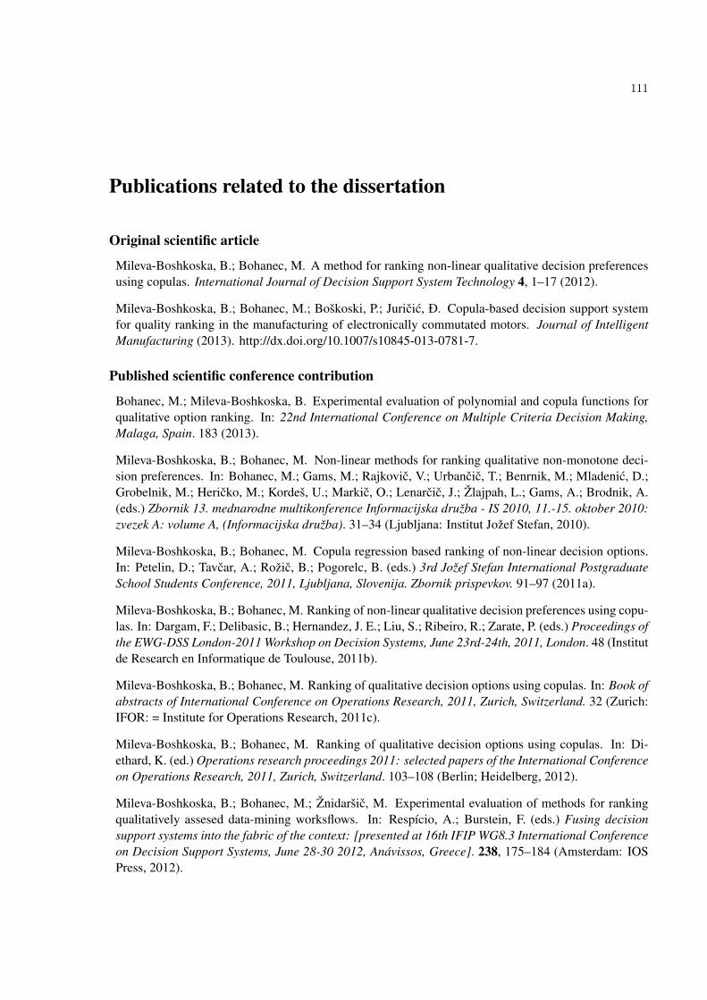
111
Publications related to the dissertation
Original scientific article
Mileva-Boshkoska, B.; Bohanec, M. A method for ranking non-linear qualitative decision preferencesusing copulas. International Journal of Decision Support System Technology 4, 1–17 (2012).
Mileva-Boshkoska, B.; Bohanec, M.; Boškoski, P.; Juricic, Ð. Copula-based decision support systemfor quality ranking in the manufacturing of electronically commutated motors. Journal of IntelligentManufacturing (2013). http://dx.doi.org/10.1007/s10845-013-0781-7.
Published scientific conference contribution
Bohanec, M.; Mileva-Boshkoska, B. Experimental evaluation of polynomial and copula functions forqualitative option ranking. In: 22nd International Conference on Multiple Criteria Decision Making,Malaga, Spain. 183 (2013).
Mileva-Boshkoska, B.; Bohanec, M. Non-linear methods for ranking qualitative non-monotone deci-sion preferences. In: Bohanec, M.; Gams, M.; Rajkovic, V.; Urbancic, T.; Benrnik, M.; Mladenic, D.;Grobelnik, M.; Hericko, M.; Kordeš, U.; Markic, O.; Lenarcic, J.; Žlajpah, L.; Gams, A.; Brodnik, A.(eds.) Zbornik 13. mednarodne multikonference Informacijska družba - IS 2010, 11.-15. oktober 2010:zvezek A: volume A, (Informacijska družba). 31–34 (Ljubljana: Institut Jožef Stefan, 2010).
Mileva-Boshkoska, B.; Bohanec, M. Copula regression based ranking of non-linear decision options.In: Petelin, D.; Tavcar, A.; Rožic, B.; Pogorelc, B. (eds.) 3rd Jožef Stefan International PostgraduateSchool Students Conference, 2011, Ljubljana, Slovenija. Zbornik prispevkov. 91–97 (2011a).
Mileva-Boshkoska, B.; Bohanec, M. Ranking of non-linear qualitative decision preferences using copu-las. In: Dargam, F.; Delibasic, B.; Hernandez, J. E.; Liu, S.; Ribeiro, R.; Zarate, P. (eds.) Proceedings ofthe EWG-DSS London-2011 Workshop on Decision Systems, June 23rd-24th, 2011, London. 48 (Institutde Research en Informatique de Toulouse, 2011b).
Mileva-Boshkoska, B.; Bohanec, M. Ranking of qualitative decision options using copulas. In: Book ofabstracts of International Conference on Operations Research, 2011, Zurich, Switzerland. 32 (Zurich:IFOR: = Institute for Operations Research, 2011c).
Mileva-Boshkoska, B.; Bohanec, M. Ranking of qualitative decision options using copulas. In: Di-ethard, K. (ed.) Operations research proceedings 2011: selected papers of the International Conferenceon Operations Research, 2011, Zurich, Switzerland. 103–108 (Berlin; Heidelberg, 2012).
Mileva-Boshkoska, B.; Bohanec, M.; Žnidaršic, M. Experimental evaluation of methods for rankingqualitatively assesed data-mining worksflows. In: Respício, A.; Burstein, F. (eds.) Fusing decisionsupport systems into the fabric of the context: [presented at 16th IFIP WG8.3 International Conferenceon Decision Support Systems, June 28-30 2012, Anávissos, Greece]. 238, 175–184 (Amsterdam: IOSPress, 2012).

112 Publications related to the dissertation

113
Index of figures
1.1 Organization of the thesis . . . . . . . . . . . . . . . . . . . . . . . . . . . . . . . . . . 4
3.1 Hierarchy of attributes for evaluation of cars . . . . . . . . . . . . . . . . . . . . . . . . 153.2 Three stages of the QQ method . . . . . . . . . . . . . . . . . . . . . . . . . . . . . . . 163.3 Estimated regression curves obtained with QQ for options given in Table 2.2 . . . . . . . 18
4.1 Gini index is calculated as a ratio between the Lorenz curve and the perfect equality line 224.2 Regression curves obtained with different weights estimation in QQ . . . . . . . . . . . 274.3 Regression curve obtained with CIPER for the running example . . . . . . . . . . . . . 304.4 Regression curve obtained with New CIPER for the running example . . . . . . . . . . . 31
5.1 Inverse distribution function F−1(u) . . . . . . . . . . . . . . . . . . . . . . . . . . . . 365.2 Probability integral transform of a random variable X with PDF f (x) and CDF F(x) . . . 375.3 Clayton copula distribution function C(u1,u2) . . . . . . . . . . . . . . . . . . . . . . . 415.4 Clayton copula density function c(u1,u2) . . . . . . . . . . . . . . . . . . . . . . . . . 415.5 Fully nested Archimedean constructions of multi-dimensional copulas . . . . . . . . . . 455.6 Three permutations of the input variables . . . . . . . . . . . . . . . . . . . . . . . . . 455.7 Partially nested Archimedean constructions with five attributes . . . . . . . . . . . . . . 465.8 Smoothing of distribution function . . . . . . . . . . . . . . . . . . . . . . . . . . . . . 475.9 Smoothing of inverse distribution function . . . . . . . . . . . . . . . . . . . . . . . . . 485.10 Smoothing of density function . . . . . . . . . . . . . . . . . . . . . . . . . . . . . . . 48
6.1 Copula-based regression curves for different values of θ in (6.2) . . . . . . . . . . . . . 506.2 Clayton qth quantile curves (for q = 0.1,0.2, ...,0.9): (a) for (u,v) and (b) for (X ,Y )
under hypothesis for uniform margins and for θ = 0.7 . . . . . . . . . . . . . . . . . . . 516.3 Frank qth quantile curves (for q = 0.1,0.2, ...,0.9): (a) for (u,v) and (b) for (X ,Y ) under
hypothesis for Student margins with two degrees of freedom and for θ = 2.5 . . . . . . . 516.4 Frank qth quantile curves (for q = 0.1,0.2, ...,0.9): (a) for (u,v) and (b) for (X ,Y ) under
hypothesis for Student margins with two degrees of freedom and for θ =−2.5 . . . . . . 526.5 Gumble qth quantile curves (for q = 0.01,0.05,0.25,0.5,0.75,0.95,0.99): (a) for (u,v)
and (b) for (X ,Y ) under hypothesis for uniform margins and for θ = 5.7681 . . . . . . . 526.6 Frank copula contours curves: (a) for θ =−2.25 and (b) for θ = 2.25 under hypothesis
for Student margins with two degrees of freedom . . . . . . . . . . . . . . . . . . . . . 526.7 Clayton copula contours curves for θ = 5.7 under hypothesis for uniform margins . . . . 536.8 Gumbel copula contours curves for θ = 5.7 under hypothesis for uniform margins . . . . 536.9 Regression curves obtained with FNAC built with Clayton bi-variate copulas . . . . . . 586.10 Contours of the regression curves given in Figure 6.9. . . . . . . . . . . . . . . . . . . . 58

114
7.1 Percentage of fully ranked and monotonic decision tables obtained with different meth-ods on dataset 1 . . . . . . . . . . . . . . . . . . . . . . . . . . . . . . . . . . . . . . . 67
7.2 Percentage of fully ranked and monotonic decision tables obtained with different meth-ods on dataset 2 . . . . . . . . . . . . . . . . . . . . . . . . . . . . . . . . . . . . . . . 68
7.3 Percentage of fully ranked and monotonic decision tables obtained with different meth-ods on dataset 3 . . . . . . . . . . . . . . . . . . . . . . . . . . . . . . . . . . . . . . . 68
7.4 FNAC with four variables . . . . . . . . . . . . . . . . . . . . . . . . . . . . . . . . . . 697.5 Union of PNACs and FNACs . . . . . . . . . . . . . . . . . . . . . . . . . . . . . . . . 70
9.1 Structure of the end-quality assessment system . . . . . . . . . . . . . . . . . . . . . . 819.2 Bearing dimensions used for the calculation of the bearing’s characteristic frequencies . 839.3 From qualitative attributes and quantitative features to final quantitative evaluation . . . . 849.4 Intervals for mapping feature values to quantitative ones . . . . . . . . . . . . . . . . . 879.5 FNAC structure for aggregation of the attribute Inner Ring . . . . . . . . . . . . . . . . 879.6 The prototype assessment point . . . . . . . . . . . . . . . . . . . . . . . . . . . . . . . 899.7 Rankings obtained with Frank FNAC . . . . . . . . . . . . . . . . . . . . . . . . . . . . 909.8 Rankings obtained with one-parametric Clayton copula . . . . . . . . . . . . . . . . . . 909.9 Differences in rankings between models built with different quantiles q and QQ, and the
selected model built with q = 0.5 . . . . . . . . . . . . . . . . . . . . . . . . . . . . . . 919.10 Example of a workflow for a collaborative filtering recommender system (Antulov, 2011;
Bošnjak et al., 2011) . . . . . . . . . . . . . . . . . . . . . . . . . . . . . . . . . . . . 939.11 Example of DEX hierarchical tree for assessment of data-mining workflows . . . . . . . 93

115
Index of tables
2.1 Qualitative decision table . . . . . . . . . . . . . . . . . . . . . . . . . . . . . . . . . . 112.2 Quantitative decision table . . . . . . . . . . . . . . . . . . . . . . . . . . . . . . . . . 11
3.1 DEXi model tree and attribute scales for assessment of cars . . . . . . . . . . . . . . . . 153.2 Car aggregation . . . . . . . . . . . . . . . . . . . . . . . . . . . . . . . . . . . . . . . 163.3 Costs aggregation . . . . . . . . . . . . . . . . . . . . . . . . . . . . . . . . . . . . . . 163.4 Safety aggregation . . . . . . . . . . . . . . . . . . . . . . . . . . . . . . . . . . . . . 163.5 Mapping to quantitive aggregation table of Car . . . . . . . . . . . . . . . . . . . . . . 173.6 Mapping to quantitive aggregation table of Costs . . . . . . . . . . . . . . . . . . . . . 173.7 Mapping to quantitive aggregation table of Safety . . . . . . . . . . . . . . . . . . . . . 173.8 Quantitative ranking of options . . . . . . . . . . . . . . . . . . . . . . . . . . . . . . . 19
4.1 Contingency table, xi0, x j0 and x00 between a1 ∈ A1 and ci ∈C for the running examplein Table 2.2 . . . . . . . . . . . . . . . . . . . . . . . . . . . . . . . . . . . . . . . . . 24
4.2 Contingency table, xi0, x j0 and x00 between a2 ∈ A2 and ci ∈C for the running examplein Table 2.2 . . . . . . . . . . . . . . . . . . . . . . . . . . . . . . . . . . . . . . . . . 25
4.3 Quantitative ranking of options with different impurity functions . . . . . . . . . . . . . 264.4 Ranking obtained with CIPER for the running example . . . . . . . . . . . . . . . . . . 304.5 Ranking obtained with New CIPER for the running example . . . . . . . . . . . . . . . 304.6 Ranking of options with constraint optimization . . . . . . . . . . . . . . . . . . . . . . 33
5.1 Different Archimedean copulas, their generator functions ϕ , borders of θ parameter andvalue of regression variable v . . . . . . . . . . . . . . . . . . . . . . . . . . . . . . . 40
5.2 Kendall’s tau (Nelsen, 2006) . . . . . . . . . . . . . . . . . . . . . . . . . . . . . . . . 425.3 Values of θi parameters obtained with FNACs for the example in Table 2.2 . . . . . . . . 44
6.1 Number of PNAC structures depending on the number of attributes . . . . . . . . . . . . 576.2 Quantitative ranking of options . . . . . . . . . . . . . . . . . . . . . . . . . . . . . . . 576.3 Parameters of copula-based models for evaluation of car . . . . . . . . . . . . . . . . . 636.4 Option rankings of Car . . . . . . . . . . . . . . . . . . . . . . . . . . . . . . . . . . . 646.5 Option rankings of Costs . . . . . . . . . . . . . . . . . . . . . . . . . . . . . . . . . . 646.6 Option rankings of Safety . . . . . . . . . . . . . . . . . . . . . . . . . . . . . . . . . 64
7.1 Input attributes of the decision tables used in dataset 3 . . . . . . . . . . . . . . . . . . . 667.2 Percentage of monotonic and fully ranked decision tables by different methods . . . . . 677.3 Example 1 of fully ranked options only with copula functions . . . . . . . . . . . . . . . 727.4 Example 2 of fully ranked options only with copula functions . . . . . . . . . . . . . . . 727.5 Time execution in seconds of different methods averaged over 100 calculations . . . . . 73

116
8.1 Rankings obtained by different methods . . . . . . . . . . . . . . . . . . . . . . . . . . 768.2 Permutations and values of θi parameters obtained with FNACs . . . . . . . . . . . . . . 768.3 Rankings obtained with QQ and Frank copula using the PNAC given in Figure 5.7a,
before and after applying equations (3.3)–(3.5) . . . . . . . . . . . . . . . . . . . . . . 778.4 Utility function (A–D) and mapping from the qualitative attributes into quantitative ones
(A1–D1). Basic attributes are: A–Generality, B–Scalability and C–NoiseSensitivity.The aggregated attribute is D–Robustness. . . . . . . . . . . . . . . . . . . . . . . . . . 78
8.5 Option evaluation using QQ method and Clayton, Frank and Gumbel copulas . . . . . . 798.6 Ranks of options using QQ and FNACs based on Clayton, Frank and Gumbel bi-variate
copula . . . . . . . . . . . . . . . . . . . . . . . . . . . . . . . . . . . . . . . . . . . . 80
9.1 Bearing frequencies (Tandon and Choudhury, 1999) . . . . . . . . . . . . . . . . . . . . 839.2 DEX model tree and qualitative and quantitative evaluations of EC motors 744 and 9 . . 859.3 Expert defined rules for aggregation of the attribute Inner ring and mapping from the
qualitative attribute values into quantitative ones. . . . . . . . . . . . . . . . . . . . . . 869.4 DEXi model tree and attribute scales for assessment of data-mining workflows . . . . . . 949.5 Aggregation of the attribute Size . . . . . . . . . . . . . . . . . . . . . . . . . . . . . . 959.6 Quantitative mapping of the attribute Size . . . . . . . . . . . . . . . . . . . . . . . . . 959.7 Utility function (A-D) and mapping from the qualitative attributes into quantitative ones
(A1 - D1). Basic attributes are: A - Generality, B - Scalability and C - NoiseSensitivity.The aggregated attribute is D - Robustness. . . . . . . . . . . . . . . . . . . . . . . . . 96
9.8 Example of workflow options . . . . . . . . . . . . . . . . . . . . . . . . . . . . . . . . 979.9 Evaluation of different workflows using one-parametric Frank copula . . . . . . . . . . 97
1 Distribution of full ranking results of tables with two input and one output attributes . . . 1192 Distribution of full ranking results of tables with three input and one output attribute. . . 1193 Distribution of full ranking results of tables with four input and one output attributes . . 1194 Distribution of the tables solved with copulas with four input and one output attribute . . 1205 Time execution in seconds of different methods averaged over 100 calculations . . . . . 1206 Polynomial interpolation with CIPER . . . . . . . . . . . . . . . . . . . . . . . . . . . 1207 Polynomial interpolation with CIPER NEW . . . . . . . . . . . . . . . . . . . . . . . . 1208 Percentage of fully ranked tables obtained with QQ modified with impurity functions . . 1209 Rankings obtained by different methods: FNACs solves the breaching monotonicity . . . 12110 Fulfillment of properties by different methods for the example in Table 9 . . . . . . . . . 12211 Rankings obtained by different methods: PNACs solves the breaching monotonicity . . . 12212 Fulfillment of properties by different methods for the example in Table 11 . . . . . . . . 12313 Rankings obtained by different methods: symmetric attributes . . . . . . . . . . . . . . 12414 Fulfillment of properties by different methods for the example in Table 13 . . . . . . . . 125

117
Index of algorithms
1 Calculations of weights kc and nc in QQ method . . . . . . . . . . . . . . . . . . . . . . 182 Calculation of weights wi with impurity function . . . . . . . . . . . . . . . . . . . . . 253 Implementation algorithm . . . . . . . . . . . . . . . . . . . . . . . . . . . . . . . . . 594 Branching the algorithm for search of a valid hierarchical copula . . . . . . . . . . . . . 605 Search algorithm for a valid FNAC . . . . . . . . . . . . . . . . . . . . . . . . . . . . . 606 Regression using bi-variate copula . . . . . . . . . . . . . . . . . . . . . . . . . . . . . 617 Regression algorithm for FNAC structure and dependent variable in the p position . . . . 618 Regression algorithm for FNAC structure and dependent variable in the p position for
Clayton copula . . . . . . . . . . . . . . . . . . . . . . . . . . . . . . . . . . . . . . . 629 Calculate kc and nc for copula-based regression algorithm . . . . . . . . . . . . . . . . . 6210 Option evaluation using copula-based algorithm . . . . . . . . . . . . . . . . . . . . . . 62

118

119
Appendix
A Distribution of results with different tables
No. Method Fully ranked (%) Breachedmonotonicity (%)
1 QQ 8.90 91.102 Frank 49.72 03 Gumbel 63.56 04 Clayton 36.18 05 All copulas 73.23 0
Table 1: Distribution of full ranking results of tables with two input and one output attributes
No. Method Fully ranked (%) Breachedmonotonicity (%)
1 QQ 5.20 94.802 Frank 41.14 03 Gumbel 20.00 04 Clayton 26.10 05 All Copulas 52.44 0
Table 2: Distribution of full ranking results of tables with three input and one output attribute.
No. Method Fully ranked (%) Breachedmonotonicity(%)
1 QQ 0.09 99.912 Frank 84.01 03 Gumbel 80.00 04 Clayton 96.38 05 All Copulas 99.03 0
Table 3: Distribution of full ranking results of tables with four input and one output attributes

Copula type Constructed tables (%) Full ranking (%)
Clayton FNAC 84.21 84.21Clayton PNAC 14.71 12.26
Frank FNAC 83.03 83.03Frank PNAC 1.91 1.91
Gumbel FNAC 78.98 78.98Gumbel PNAC 1.3 1.13
Table 4: Distribution of the tables solved with copulas with four input and one output attribute
No. of dataset No. of tables # obtained solutions (%) Monotonicity fulfilled (%)
1 19 683 0.4014 0.15752 2 278 734 0 03 1 000 000 0 0
Table 5: Time execution in seconds of different methods averaged over 100 calculations
No. of dataset No. of tables Monotonic (%) # solutions fulfilling monotonicityand without ties (%)
1 19 683 79.08 0.82302 2 278 734 89.79 0.00183 1 000 000 59.69 0
Table 6: Polynomial interpolation with CIPER
No. of dataset No. of tables Monotonic (%) # solutions fulfilling monotonicityand without ties (%)
1 19 683 16.99 14.882 2 278 734 0.0006 0.00013 1 000 000 0.01 0.01
Table 7: Polynomial interpolation with CIPER NEW
Table 8: Percentage of fully ranked tables obtained with QQ modified with impurity functions
Method Dataset 1 (%) Dataset 2 (%) Dataset 3 (%)
gB 67.23 66.64 86.84gC 30.65 11.79 57.67gP 93.08 96.57 99.91IG 75.85 80.61 95.76χ2 77.71 66.64 86.84

Appendix 121
B Illustrative examples: rankings with different methods
This Appendix provides results from different methods on the examples provided in Chapter 8, whichare provided in Tables 9, 11 and 13. For each result, the three properties are checked: monotonicity (2.3),full ranking (2.4) and consistency (2.5), which are given in Tables 10, 12 and 14. Bolded numbers inTables 9, 11 and 13 represent ties in the results.
B.1 Appendix to Section 8.1
Table 9 gives the rankings obtained with modified QQ methods, CIPER and New CIPER, while Table 10tells which of the properties: monotonicity (2.3), full ranking (2.4) and consistency (2.5), are fulfilled byeach method. None of the methods fulfill all three properties.
Table 9: Rankings obtained by different methods: FNACs solves the breaching monotonicity
No. A1 A2 A3 A4 Cls gB gCov gPop InfG χ2 CIP. New CIP.
1 4 2 5 1 1 0.8125 1.1667 0.9463 0.8354 0.8125 3 2.04162 4 5 3 2 1 1.2344 0.6806 1.1707 1.2273 1.2344 3 2.95053 2 2 3 4 1 0.7656 0.8056 0.7824 0.7727 0.7656 3 3.02654 3 1 5 4 1 0.9375 1.3194 1.0995 0.9739 0.9375 3 1.63425 3 2 4 5 1 1.1406 1.1250 1.2176 1.1666 1.1406 3 2.42366 2 4 1 1 2 1.7832 1.6327 1.7224 1.7699 1.7832 3 3.17667 4 1 4 1 2 1.8363 2.2653 1.9304 1.8528 1.8363 3 2.36538 2 1 2 2 2 1.6504 1.9184 1.6667 1.6538 1.6504 3 3.44819 5 5 1 4 2 2.3496 1.8469 2.2995 2.3462 2.3496 3 3.298110 1 4 5 5 2 2.2345 2.3673 2.3333 2.2496 2.2345 3 2.878111 3 5 1 2 3 2.7931 2.6368 2.7402 2.7838 2.7931 3 2.812212 5 1 4 3 3 2.8793 3.3632 3.0500 2.9300 2.8793 3 2.792413 2 5 5 3 3 3.2069 3.2684 3.2598 3.2162 3.2069 3 2.784814 3 4 2 5 3 3.1897 2.9526 3.1207 3.1869 3.1897 3 2.981315 2 3 4 5 3 3.0690 3.2579 3.1501 3.0945 3.0690 3 2.677116 5 3 3 1 4 3.8033 4.0047 3.8442 3.8122 3.8033 3 3.375317 1 4 1 3 4 3.6393 3.6215 3.6312 3.6376 3.6393 3 3.588318 4 3 2 3 4 3.8279 3.9019 3.8389 3.8329 3.8279 3 3.326119 3 3 3 3 4 3.8033 4.0047 3.8442 3.8122 3.8033 3 2.950620 5 5 5 5 4 4.3607 4.3785 4.3688 4.3624 4.3607 3 3.092721 1 1 1 1 5 4.6250 4.6512 4.6250 4.6250 4.6250 3 4.145122 5 2 2 2 5 5.0735 5.0233 5.0627 5.0744 5.0735 3 3.774023 1 3 2 2 5 4.8824 4.8023 4.8697 4.8780 4.8824 3 3.642724 1 2 3 4 5 4.9853 5.1047 5.0051 4.9891 4.9853 3 3.373925 4 4 4 4 5 5.3750 5.3488 5.3750 5.3750 5.3750 3 2.8397

122 Appendix
Table 10: Fulfillment of properties by different methods for the example in Table 9
Method Monotonicity (2.3) Full ranking (2.4) Consistency (2.5)
gB yes no yesgC yes no yesgP yes no yesIG yes no yesχ2 yes no yes
CIPER yes no noNew CIPER no yes no
B.2 Appendix to Section 8.2
Table 11 gives the rankings obtained with modified QQ methods, CIPER and New CIPER, while Table 12tells which of the properties: monotonicity (2.3), full ranking (2.4) and consistency (2.5), are fulfilled byeach method. None of the methods fulfill all three properties.
Table 11: Rankings obtained by different methods: PNACs solves the breaching monotonicity
No. A1 A2 A3 A4 Cls gB gCov gPop InfG χ2 CIP. New CIP.
1 2 4 1 1 1 0.7079 0.6303 0.7108 0.7104 0.7079 3 3.81702 5 2 2 2 1 1.0787 1.0806 1.0630 1.0728 1.0787 3 2.56333 5 1 4 3 1 1.2921 1.3602 1.2892 1.2896 1.2921 3 1.98894 2 2 3 4 1 1.0787 1.0806 1.0493 1.0807 1.0787 3 2.90015 3 1 5 4 1 1.2809 1.3697 1.2815 1.2848 1.2809 3 2.23676 4 2 5 1 2 1.8814 2.1516 1.9219 1.8838 1.8814 3 2.56637 2 1 2 2 2 1.6186 1.7254 1.6182 1.6184 1.6186 3 3.06948 4 4 4 4 2 2.1442 2.0533 2.1454 2.1447 2.1442 3 2.78119 1 4 5 5 2 2.0737 1.9631 2.0790 2.0797 2.0737 3 3.120010 5 5 5 5 2 2.3814 2.2746 2.3818 2.3816 2.3814 3 2.520511 4 3 2 3 3 2.8475 2.7778 2.8301 2.8413 2.8475 3 2.918112 3 3 3 3 3 2.8136 2.8120 2.8278 2.8152 2.8136 3 3.024413 3 4 2 5 3 3.1864 2.7350 3.1341 3.1848 3.1864 3 3.050814 3 2 4 5 3 3.1864 3.2650 3.1722 3.1848 3.1864 3 2.358715 2 3 4 5 3 3.1525 3.0342 3.1508 3.1587 3.1525 3 2.800616 5 3 3 1 4 3.9635 4.1394 4.0309 3.9627 3.9635 3 2.771417 4 1 4 1 4 3.7760 4.3333 3.8475 3.7738 3.7760 3 2.452618 1 4 1 3 4 3.6927 3.6667 3.6977 3.6947 3.6927 3 3.851719 2 5 5 3 4 4.2135 4.0727 4.3023 4.2291 4.2135 3 3.494220 5 5 1 4 4 4.3073 3.9636 4.3023 4.3053 4.3073 3 3.237721 1 1 1 1 5 4.6468 4.8661 4.6439 4.6465 4.6468 3 3.459022 3 5 1 2 5 5.1468 4.7165 5.1314 5.1465 5.1468 3 3.814323 1 3 2 2 5 4.9246 4.8661 4.9223 4.9273 4.9246 3 3.662324 4 5 3 2 5 5.3532 5.0866 5.3561 5.3535 5.3532 3 3.426325 1 2 3 4 5 5.0992 5.2835 5.0735 5.0991 5.0992 3 3.1363

Appendix 123
Table 12: Fulfillment of properties by different methods for the example in Table 11
Method Monotonicity (2.3) Full ranking (2.4) Consistency (2.5)
gB yes no yesgC no no yesgP yes no yesIG yes no yesχ2 yes no yes
CIPER yes no noNew CIPER no yes no

124 Appendix
B.3 Appendix to Section 8.3
Table 13 gives the rankings obtained with modified QQ methods, CIPER and New CIPER, while Table 14tells which of the properties: monotonicity (2.3), full ranking (2.4) and consistency (2.5), are fulfilled byeach method. Only New CIPER fulfills all three properties.
Table 13: Rankings obtained by different methods: symmetric attributes
No. A1 A2 A3 Cls gB gCov gPop InfG χ2 CIP. New CIP.
1 1 1 1 1 1.0000 1.0000 1.0000 1.0000 1.0000 1.1111 1.25592 2 1 1 2 1.8750 1.8750 1.8750 1.8750 1.8750 1.6667 1.73333 3 1 1 2 2.1250 2.1250 2.1250 2.1250 2.1250 2.2222 2.23794 1 2 1 2 1.8750 1.8750 1.8750 1.8750 1.8750 1.6667 1.75875 2 2 1 2 2.1250 2.1250 2.1250 2.1250 2.1250 2.2222 2.26706 1 3 1 2 2.1250 2.1250 2.1250 2.1250 2.1250 2.2222 2.28927 1 1 2 2 1.8750 1.8750 1.8750 1.8750 1.8750 1.6667 1.70238 2 1 2 2 2.1250 2.1250 2.1250 2.1250 2.1250 2.2222 2.20169 1 2 2 2 2.1250 2.1250 2.1250 2.1250 2.1250 2.2222 2.209810 1 1 3 2 2.1250 2.1250 2.1250 2.1250 2.1250 2.2222 2.175811 3 2 1 3 2.8750 2.8750 2.8750 2.8750 2.8750 2.7778 2.802512 2 3 1 3 2.8750 2.8750 2.8750 2.8750 2.8750 2.7778 2.828313 3 3 1 3 3.1250 3.1250 3.1250 3.1250 3.1250 3.3333 3.394614 3 1 2 3 2.8750 2.8750 2.8750 2.8750 2.8750 2.7778 2.728015 2 2 2 3 2.8750 2.8750 2.8750 2.8750 2.8750 2.7778 2.744616 3 2 2 3 3.1250 3.1250 3.1250 3.1250 3.1250 3.3333 3.306617 1 3 2 3 2.8750 2.8750 2.8750 2.8750 2.8750 2.7778 2.744918 2 3 2 3 3.1250 3.1250 3.1250 3.1250 3.1250 3.3333 3.315219 2 1 3 3 2.8750 2.8750 2.8750 2.8750 2.8750 2.7778 2.697020 3 1 3 3 3.1250 3.1250 3.1250 3.1250 3.1250 3.3333 3.245321 1 2 3 3 2.8750 2.8750 2.8750 2.8750 2.8750 2.7778 2.688022 2 2 3 3 3.1250 3.1250 3.1250 3.1250 3.1250 3.3333 3.249323 1 3 3 3 3.1250 3.1250 3.1250 3.1250 3.1250 3.3333 3.227824 3 3 2 4 4.0000 4.0000 4.0000 4.0000 4.0000 3.8889 3.912825 3 2 3 4 4.0000 4.0000 4.0000 4.0000 4.0000 3.8889 3.837926 2 3 3 4 4.0000 4.0000 4.0000 4.0000 4.0000 3.8889 3.829327 3 3 3 5 5.0000 5.0000 5.0000 5.0000 5.0000 4.4444 4.4580

Appendix 125
Table 14: Fulfillment of properties by different methods for the example in Table 13
Method Monotonicity (2.3) Full ranking (2.4) Consistency (2.5)
gB yes no yesgC yes no yesgP yes no yesIG yes no yesχ2 yes no yes
CIPER yes no yesNew CIPER yes yes yes

C Specific derivations for multi-variate Frank and Gumbel copulas
C.1 Specific derivation for multi-variate Frank copula
The generator function
ϕ(x) =− ln(
e−θx−1e−θ −1
). (1)
First derivative of the generator (1)
dϕ
dx=
θe−θx
e−θx−1.
The inverse generator for Frank copula is:
ϕ−1(x) = 1+
x− ln(1− eθ + eθ+x
)θ
. (2)
Finally, the derivative of the inverse generator (2) of order i is:
diϕ−1
dxi =eθ −1
θ
eθ+x
(eθ − eθ+x−1)i
×i−1
∑j=1
Bi−1, je(i− j−1)(θ+x)(
eθ −1) j−1
,
where Bi, j = (i− j+1)Bi−1, j−1 + jBi−1, j and Bi1 = Bii = 1.
C.2 Specific derivation for multi-variate Gumbel copula
The generator function of Gumbel copula is given with:
ϕ(x) = (− lnx)θ . (3)
The first derivative of the generator (3)
dϕ
dx=
(− lnx)θ θ
x lnx.
The inverse generator function is:
ϕ−1(x) = exp
(−x1/θ
). (4)
The first derivative of (4) is:
ϕ−1[1] =
e−x1θ x
1θ−1
θ.
The second derivative of (4) is:
ϕ−1[2] =
e−x1θ x
2θ−2
θ 2 −( 1
θ−1)
e−x1θ x
1θ−2
θ.

Appendix 127
Third derivative of (4) is:
ϕ−1[3] =−e−x
1θ x
3θ−3
θ 3 +
( 1θ−1)
e−x1θ x
2θ−3
θ 2
+
( 2θ−2)
e−x1θ x
2θ−3
θ 2 −( 1
θ−2)( 1
θ−1)
e−x1θ x
1θ−3
θ.
Fourth derivative of (4) is:
ϕ−1[4] =
1θ 4
{e−x
1θ x
1θ−4
×[6θ
3 +11θ2(
x1θ −1
)+ x3/θ −6x2/θ
+7x1θ +6θ
(x2/θ −3x
1θ +1
)−1]}
.
Fifth derivative of (4) is:
ϕ−1[5] =
1θ 5
{e−x
1θ x
1θ−5
×[−24θ
4−50θ3(
x1θ −1
)−35θ
2(
x2/θ −3x1θ +1
)−x4/θ +10x3/θ −25x2/θ +15x
1θ −10θ
(x3/θ −6x2/θ +7x
1θ −1
)−1]}
.

D Biography
Biljana Mileva Boshkoska was born on 11 January 1979 in Skopje, Macedonia. She has completed thesecondary education at Nikola Karev gymnasium in Skopje, and obtained a diploma and a master degreeat the Faculty of Electrical Engineering and Information Technologies in Skopje in 2002 and 2008. Sheworked on several EU projects on environment and vocational education from 2002–2006. She workedas a teaching assistant at the Faculty of Electrical Engineering and Information Technologies until 2009.In 2009 she started her PhD at the Jožef Stefan Postgraduate School under the supervision of Prof.Dr. Marko Bohanec. The results of her research work are published in several journal and conferencepublications.