Embed Size (px)
Citation preview

Finite Element Modelling
of Anular Lesions
in the
Lumbar Intervertebral
Disc
J. Paige Little, B.E. (Mechanical)(Hons)
Submitted for the award of degree of Doctor of Philosophy in
The Centre for Built Environment and Engineering Research,
School of Mechanical, Manufacturing and Medical Engineering,
Queensland University of Technology.

iii
KKeeyywwoorrddss Spine, intervertebral disc, degeneration, anular lesions, finite element analysis,
hyperelastic material model, biomechanics

iv
AAbbssttrraacctt Low back pain is an ailment that affects a significant portion of the community.
However, due to the complexity of the spine, which is a series of interconnected
joints, and the loading conditions applied to these joints the causes for back pain are
not well understood. Investigations of damage or failure of the spinal structures from
a mechanical viewpoint may be viewed as a way of providing valuable information
for the causes of back pain. Low back pain is commonly associated with injury to, or
degeneration of, the intervertebral discs and involves the presence of tears or lesions
in the anular disc material. The aim of the study presented in this thesis was to
investigate the biomechanical effect of anular lesions on disc function using a finite
element model of the L4/5 lumbar intervertebral disc.
The intervertebral disc consists of three main components – the anulus fibrosus, the
nucleus pulposus and the cartilaginous endplates. The anulus fibrosus is comprised of
collagen fibres embedded in a ground substance while the nucleus is a gelatinous
material. The components of the intervertebral disc were represented in the model
together with the longitudinal ligaments that are attached to the anterior and posterior
surface of the disc. All other bony and ligamentous structures were simulated through
the loading and boundary conditions.
A high level of both geometric and material accuracy was required to produce a
physically realistic finite element model. The geometry of the model was derived
from images of cadaveric human discs and published data on the in vivo configuration
of the L4/5 disc. Material properties for the components were extracted from the
existing literature. The anulus ground substance was represented as a Mooney-Rivlin
hyperelastic material, the nucleus pulposus was modelled as a hydrostatic fluid in the
healthy disc models and the cartilaginous endplates, collagen fibres and longitudinal
ligaments were represented as linear elastic materials. A preliminary model was
developed to assess the accuracy of the geometry and material properties of the disc
components. It was found that the material parameters defined for the anulus ground
substance did not accurately describe the nonlinear shear behaviour of the tissue.
Accurate representation this nonlinear behaviour was thought to be important in

v
ensuring the deformations observed in the anulus fibrosus of the finite element model
were correct.
There was no information found in the literature on the mechanical properties of the
anulus ground substance. Experimentation was, therefore, carried out on specimens
of sheep anulus fibrosus in order to quantify the mechanical response of the ground
substance. Two testing protocols were employed. The first series of tests were
undertaken to provide information on the strain required to initiate permanent damage
in the ground substance. The second series of tests resulted in the acquisition of data
on the mechanical response of the tissue to repeated loading. The results of the
experimentation carried out to determine the strain necessary to initiate permanent
damage suggested that during daily loading some derangement might be caused in the
anulus ground substance. The results for the mechanical response of the tissue were
used to determine hyperelastic constants which were incorporated in the finite
element model. A second order Polynomial and a third order Ogden strain energy
equation were used to define the anulus ground substance. Both these strain energy
equations incorporated the nonlinear mechanical response of the tissue during shear
loading conditions.
Using these geometric data and material properties a finite element model of a
representative L4/5 intervertebral disc was developed.
When the measured material parameters for the anulus ground substance were
implemented in the finite element model, large deformations were observed in the
anulus fibrosus and excessive nucleus pressures were found. This suggested that the
material parameters defining the anulus ground substance were overly compliant and
in turn, implied the possibility that the stiffness of the sheep anulus ground substance
was lower than the stiffness of the human tissue. Even so, the mechanical properties
of the sheep joints had been shown to be similar to those of the human joint and it was
concluded that the results of analyses using these parameters would provide valuable
qualitative information on the disc mechanics.
To represent the degeneration of the anulus fibrosus, the models included simulations
of anular lesions – rim, radial and circumferential lesions. Degeneration of the

vi
nucleus may be characterised by a significant reduction in the hydrostatic nucleus
pressure and a loss of hydration. This was simulated by removal of the hydrostatic
nucleus pressure.
Analyses were carried out using rotational loading conditions that were comparable to
the ranges of motion observed physiologically. The results of these analyses showed
that the removal of the hydrostatic nucleus pressure from an otherwise healthy disc
resulted in a significant reduction in the stiffness of the disc. This indicated that when
the nucleus pulposus is extremely degenerate, it offers no resistance to the
deformation of the anulus and the mechanics of the disc are significantly changed.
Specifically, the resistance to rotation offered by the intervertebral disc is reduced,
which may affect the stability of the joint. When anular lesions were simulated in the
finite element model they caused minimal changes in the peak moments resisted by
the disc under rotational loading. This suggested that the removal of the nucleus
pressure had a greater effect on the mechanics of the disc than the simulation of
anular lesions.
The results of the finite element model reproduced trends observed in both the healthy
and degenerate intervertebral disc in terms of variations in nucleus pressure with
loading conditions, axial displacement of the superior surface and bulge of the
peripheral anulus. It was hypothesised that the reduced rotational stiffness of the
degenerate disc may result in overload of the surrounding innervated
osseoligamentous anatomy which may in turn cause back pain. Similarly back pain
may result from the abnormal deformation of the innervated peripheral anulus in the
vicinity of anular lesions. Furthermore, it was hypothesised that biochemical changes
may result in the degeneration of the nucleus, which in turn may cause excessive
strains in the anulus ground substance and lead to the initiation of permanent damage
in the form of anular lesions. With further refinement of the components of the model
and the methods used to define the anular lesions it was considered that this model
would provide a powerful analysis tool for the investigation of the mechanics of
intervertebral discs with and without significant degeneration.

vii
TTaabbllee ooff CCoonntteennttss Keywords .................................................................................................................... iii
Abstract .......................................................................................................................iv
Table of Contents ......................................................................................................vii
List of Tables .......................................................................................................... xvii
List of Figures ............................................................................................................xx
List of Symbols ......................................................................................................xxvii
List of Abbreviations .......................................................................................... xxviii
Statement of Originality ........................................................................................xxix
Acknowledgements .................................................................................................xxx
1 Introduction............................................................................................................1
1.1 Aims and Objectives of the Thesis ...................................................................4
1.2 Limitations of the Study ...................................................................................5
2 Literature Review ..................................................................................................6
2.1 Spinal Anatomy ................................................................................................6
2.1.1 The bony spinal column.........................................................................7
2.1.2 The intervertebral disc ...........................................................................8
2.1.2.1 Nucleus pulposus .....................................................................9
2.1.2.2 Anulus fibrosus ........................................................................9
2.1.2.3 Cartilaginous endplates ..........................................................11
2.1.3 Anatomy and attachment of the longitudinal ligaments ......................12
2.1.3.1 Cross-sectional area ...............................................................13
2.1.3.2 Lateral width ..........................................................................15
2.1.3.3 Pre-tension in the ligaments ...................................................16
2.2 Location of the Instantaneous Centres of Rotation during Physiological
Loading...........................................................................................................16
2.2.1 Flexion and extension ..........................................................................17
2.2.2 Axial Rotation......................................................................................17
2.2.3 Lateral bending ....................................................................................18
2.3 Degeneration and Anular Lesions ..................................................................19

viii
2.3.1 The mechanism of degeneration and the initiation of anular lesions...22
2.3.2 Relevance of studying anular lesions...................................................23
2.4 The Use of FEM to Study the Spine and in particular Anular Lesions ..........23
2.5 Shortcomings in Previous Models ..................................................................24
2.6 Mechanical Properties of Components in the Spine.......................................27
2.6.1 The intervertebral disc components .....................................................27
2.6.1.1 Nucleus pulposus ...................................................................27
2.6.1.2 Anulus fibrosus and the anulus fibrosus ground substance ...28
2.6.1.3 Cartilaginous endplate............................................................29
2.6.1.4 Collagen fibres .......................................................................30
2.6.2 Incompressibility of the intervertebral disc .........................................31
2.6.3 Functional behaviour of the anulus fibrosus and nucleus pulposus.....32
2.6.3.1 The inclination of collagen fibres ..........................................33
2.6.3.2 Uniaxial compression.............................................................33
2.6.3.3 Bending ..................................................................................34
2.6.3.4 Torsion ...................................................................................34
2.6.4 Mechanical properties of the longitudinal ligaments...........................35
2.6.4.1 Average elastic modulus and spring stiffness of the anterior
longitudinal ligament .............................................................38
2.6.4.2 Average elastic modulus and spring stiffness of the posterior
longitudinal ligament .............................................................39
2.7 Use of a Hyperelastic Model for the Anulus Ground Matrix .........................40
2.7.1 Rubber elasticity theories and continuum mechanics..........................40
2.7.1.1 Strain invariants (Reference: Williams, 1973, Chapter 1;
Ugural and Fenster, 1995)......................................................40
2.7.1.2 Stress components and the strain energy equation,
(Reference: Williams, 1973, Chapter 1; Ugural and Fenster,
1995) ......................................................................................46
2.7.2 Forms and applications of the strain energy equation .........................50
2.8 Experimental Testing of the Intervertebral Disc ............................................54
2.8.1 Types of testing carried out and material information available in
literature...............................................................................................54
2.8.2 Specimen handling...............................................................................55
2.9 Conclusions ....................................................................................................58

ix
3 Development of the Preliminary FEM..............................................................60
3.1 Basic description of the FE method................................................................61
3.2 Abaqus 6.3 Finite Element Modelling Software ............................................63
3.2.1 Specifics of finite element analysis carried out using Abaqus 6.3 ......64
3.3 Geometry of the Anulus Fibrosus and Nucleus Pulposus in the Transverse
Plane ...............................................................................................................66
3.3.1 Methods – anulus boundary .................................................................67
3.3.1.1 Measurements ........................................................................67
3.3.1.2 Development of equations .....................................................69
3.3.1.3 Disc area.................................................................................73
3.3.1.4 Validation of the anulus formulae..........................................73
3.3.2 Methods – nucleus ...............................................................................74
3.3.2.1 Measurement ..........................................................................75
3.3.2.2 Development of equations .....................................................75
3.3.2.3 Nucleus area ...........................................................................76
3.3.2.4 Validation of the nucleus equations .......................................76
3.3.3 Discussion concerning the anulus and nucleus boundaries .................80
3.4 Geometry of the Collagen Fibres....................................................................82
3.4.1 Cross-sectional area of the collagen fibres ..........................................83
3.4.2 Collagen fibre spacing .........................................................................85
3.4.3 Angle of inclination of the rebar elements within the layers of collagen
fibres....................................................................................................85
3.4.4 Embedding elements............................................................................86
3.5 Determination of Sagittal Geometry...............................................................87
3.6 Location of the Instantaneous Axes of Rotation During Rotation .................87
3.6.1 Flexion/Extension ................................................................................87
3.6.2 Axial rotation .......................................................................................88
3.6.3 Lateral bending ....................................................................................89
3.7 Fortran Programming .....................................................................................90
3.8 Description of the Finite Elements Used in the FEM.....................................90
3.8.1 Anulus fibrosus and cartilaginous endplate .........................................91
3.8.2 Collagen fibres .....................................................................................92
3.8.3 Nucleus pulposus .................................................................................93
3.9 Mesh Generation using Abaqus Input Files ...................................................94

x
3.10 Material Properties.........................................................................................95
3.10.1 Collagen fibres .....................................................................................95
3.10.2 Cartilaginous endplate .........................................................................96
3.10.3 Nucleus pulposus .................................................................................97
3.10.4 Anulus fibrosus ground substance .......................................................97
3.11 Boundary Conditions and Loading...............................................................102
3.11.1 Professor Nachemson's research on spinal loading ...........................102
3.11.2 Nucleus pulposus pressurisation........................................................103
3.11.3 Modelling adjacent vertebrae.............................................................103
3.11.4 Musculature and posterior elements ..................................................105
3.11.5 Uniaxial compression loading for validating the preliminary model 106
3.11.6 Iteration to determine the initial sagittal geometry of the intervertebral
disc FEM ...........................................................................................107
3.12 Optimising the Mesh Density of the FEM...................................................108
3.13 Analysis of the FEM....................................................................................112
3.13.1 The effect of variation in the transverse profile of the anulus and
nucleus boundaries ............................................................................113
3.13.2 Response of the FEM (Specimen 50) to the 70kPa nucleus pulposus
pressure..............................................................................................120
3.13.3 Analysis of the FEM under compression...........................................121
3.13.4 Full forward flexion ...........................................................................124
3.13.4.1 Validation criterion for full flexion......................................125
3.13.4.2 Results of analysis of the FEM under full flexion ...............125
3.14 Assessment of the Accuracy of the FEM ....................................................133
4 Experimental Testing of the Anulus Fibrosus................................................137
4.1 Objectives for Testing the Anulus Fibrosus .................................................137
4.2 Mechanical Testing – Rationale and Description.........................................138
4.3 Specimen Harvesting....................................................................................141
4.4 Biaxial Compression Testing Methods and Equipment ...............................144
4.4.1 Principle of operation.........................................................................144
4.4.2 Design details and pressure vessel components.................................146
4.4.2.1 Maximum vessel pressure and design pressure ...................146
4.4.2.2 Vessel walls..........................................................................147

xi
4.4.2.3 Fasteners...............................................................................148
4.4.2.4 Viewing windows ................................................................149
4.4.2.5 Attachment of specimen to nylon cord ................................150
4.4.2.6 Leaking piston and bore insert .............................................150
4.4.2.7 Adjustment knob for accurate orientation of the specimens 154
4.4.3 Proof testing .......................................................................................155
4.4.4 Setup of equipment ............................................................................156
4.4.5 Measurement of biaxial compressive stress and strain ......................157
4.4.5.1 Choice of pressure regulator ................................................157
4.4.5.2 Profile projector ...................................................................158
4.4.5.3 Data acquisition - hydrostatic pressure and deformation.....159
4.4.6 Commissioning of pressure vessel.....................................................159
4.4.6.1 Force applied to the piston ...................................................160
4.4.6.2 Biaxial compression of EVA foam ......................................162
4.5 Uniaxial Compression and Simple Shear .....................................................164
4.5.1 Testing equipment..............................................................................164
4.5.1.1 Uniaxial compression...........................................................164
4.5.1.2 Simple shear .........................................................................165
4.5.2 Maximum strains applied during testing............................................167
4.6 Strain Rate during Uniaxial Compression and Simple Shear Loading.........167
4.6.1 Procedure for testing to determine the tissue response to varied strain
rates ...................................................................................................168
4.6.2 Results and discussion of strain rate experiments..............................169
4.6.2.1 Strain rate 0.001 sec-1...........................................................169
4.6.2.2 Strain rate 0.10 sec-1.............................................................170
4.6.2.3 Strain rate 0.01 sec-1.............................................................171
4.6.3 Discussion and justification for the choice of strain rate...................171
4.7 Results for Mechanical Testing of the Anulus Fibrosus Ground Substance 174
4.7.1 Results of initial and repeated loading – stress-strain tests................174
4.7.2 Statistical analysis..............................................................................179
4.7.2.1 Simple shear .........................................................................180
4.7.2.2 Uniaxial compression...........................................................181
4.7.2.3 Biaxial compression.............................................................182
4.7.3 Range of test data...............................................................................184

xii
4.7.4 Discussion..........................................................................................185
4.8 Pilot Study to Determine the Derangement Strain .......................................186
4.8.1 Rationale for carrying out additional experimentation ......................186
4.8.1.1 Fluid loss ..............................................................................186
4.8.1.2 Viscoelastic effects in the anulus fibrosus solid skeleton ....186
4.8.1.3 Derangement of the anulus fibrosus.....................................187
4.8.2 Testing to determine the derangement strain .....................................187
4.8.2.1 Procedure .............................................................................188
4.8.2.2 Results ..................................................................................188
4.8.2.3 Discussion of the range of derangement strain of the anulus
fibrosus ground substance....................................................192
4.8.2.4 An hypothesis for disc degeneration....................................193
4.9 Discussion of Regional Stiffness and Stiffening Mechanisms in the Anulus
Fibrosus Specimens ......................................................................................193
4.9.1 Uniaxial compression.........................................................................194
4.9.2 Simple shear.......................................................................................195
4.9.3 Biaxial compression...........................................................................196
4.9.3.1 Deformation mechanism in the radial and circumferential
regions..................................................................................196
4.9.3.2 Difference in regions of highest stiffness when measured
radially and circumferentially ..............................................197
4.9.3.3 Drop in stiffness between the initial and repeated loading and
derangement strains for biaxial compression.......................198
4.10 Discussion of Edge Effects..........................................................................199
4.11 Potential Sources of Error in the Results.....................................................201
4.12 Conclusion ...................................................................................................201
5 Determining Hyperelastic Parameters for the Anulus Fibrosus Ground
Substance ............................................................................................................203
5.1 Chapter Overview.........................................................................................203
5.2 Manipulation of Experimental Regression Lines to Obtain Input for the Strain
Energy Equations..........................................................................................205
5.2.1 Simple shear compared to pure shear (Treloar, 1975).......................205
5.2.2 Manipulating simple shear data to obtain pure shear data.................206

xiii
5.2.3 Principal extension ratios for Simple Shear deformation ..................209
5.2.4 Average biaxial compression data .....................................................212
5.3 Approach to Choosing Hyperelastic Models for the Anulus Fibrosus Ground
Substance ......................................................................................................212
5.3.1 Possible strain energy equations for the anulus fibrosus ground
substance ...........................................................................................213
5.3.1.1 Veronda and Westmann .......................................................214
5.3.1.2 Ogden ...................................................................................214
5.3.1.3 Extended Mooney equation .................................................215
5.3.1.4 Polynomial ...........................................................................215
5.3.2 Verification of the Abaqus algorithm used to determine hyperelastic
parameters .........................................................................................216
5.4 Strain Energy Equations Used for the Anulus Fibrosus Ground Substance.222
5.4.1 Inhomogeneous hyperelastic model for the ground substance ..........222
5.4.1.1 Explanation of the criterion used to select the hyperelastic
strain energy equation for the anterior, lateral and posterior
anulus during initial and repeated loading ...........................225
5.4.1.2 Inhomogeneous hyperelastic constants for initial and repeated
loading..................................................................................232
5.4.2 Homogeneous hyperelastic model for the ground substance.............232
5.5 Conclusion ....................................................................................................235
6 Implementation of the Improved Anulus Fibrosus Material Properties....236
6.1 Chapter Overview.........................................................................................236
6.2 Implementation of the Homogeneous Anulus Ground Substance into the FEM
..................................................................................................................237
6.3 Compatibility of the Material Stiffness of the Collagen Fibres and the Anulus
Fibrosus Ground Substance ..........................................................................240
6.4 Improved Element Configuration for the Hydrostatic Fluid Elements on the
Inner Anulus Fibrosus ..................................................................................241
6.4.1 Results of analysis of the Homogeneous FEM with improved
hydrostatic fluid element configuration ............................................245
6.4.2 Discussion..........................................................................................250
6.4.3 Summary ............................................................................................250

xiv
6.5 Improved Properties for the Collagen Fibres in the Anulus Fibrosus ..........251
6.5.1 Collagen fibre inclination ..................................................................252
6.5.2 Collagen fibre stiffness ......................................................................253
6.5.3 Results of the analysis of the Homogeneous FEM using improved
collagen fibre geometry and material properties...............................255
6.5.4 Discussion and conclusions ...............................................................257
6.6 Implementation of the Inhomogeneous Anulus Ground Substance into the
FEM ..............................................................................................................258
6.6.1 Results of the Inhomogeneous FEM..................................................259
6.6.2 Discussion and conclusions for the Inhomogeneous FEM................263
6.6.2.1 Posterior and posterolateral bulge of the anulus fibrosus ....263
6.6.2.2 Anterior translation and rotation of the superior surface of the
Inhomogeneous FEM...........................................................264
6.6.2.3 Compliance of the Inhomogeneous anulus fibrosus ground
substance ..............................................................................264
6.6.2.4 Method for applying compressive torso load.......................265
6.7 Discussion and Conclusions on Implementation of the Homogeneous and
Inhomogeneous Material Parameters for the Anulus Fibrosus Ground
Substance ......................................................................................................266
7 Modelling Anterior and Posterior Longitudinal Ligaments........................268
7.1 Method of Representing the Longitudinal Ligaments in the FEM...............269
7.1.1 Spring elements..................................................................................269
7.1.2 Anterior and posterior longitudinal ligament geometry.....................272
7.1.3 Crimp and pre-tension in the anterior and posterior longitudinal
ligaments ...........................................................................................272
7.1.4 Stiffness of the anterior and posterior longitudinal ligaments ...........274
7.2 Analysis of the Homogeneous FEM with Longitudinal Ligaments .............275
7.2.1 Results................................................................................................275
7.2.2 Discussion..........................................................................................279
7.3 Analysis of the Homogeneous FEM with Longitudinal Ligaments – Correct
Disc Heights .................................................................................................280
7.3.1 Results................................................................................................280
7.3.2 Discussion..........................................................................................284

xv
7.4 Analysis of the Inhomogeneous FEM with Longitudinal Ligaments...........285
7.4.1 Results and discussion of unsuccessful analyses of the Inhomogeneous
FEM...................................................................................................285
7.4.1.1 Effects of removing the 70kPa loading condition................289
7.4.2 Results of the successful analysis of the Inhomogeneous FEM using a
single loading condition of 500N compression.................................291
7.4.3 Discussion..........................................................................................295
7.5 Discussion of the Displacement Convergence Problems in the Unsuccessful
Analyses of the Inhomogeneous FEM..........................................................295
7.6 Analysis of the Inhomogeneous FEM with Longitudinal Ligaments – Correct
Disc Heights .................................................................................................296
7.6.1 Results for the Inhomogeneous FEM with longitudinal ligaments,
correct sagittal geometry and a single 500N compression loading
condition............................................................................................296
7.6.2 Conclusions with respect to the Inhomogeneous FEM......................300
7.7 Discussion of the Mechanical Properties of the Anulus Fibrosus Ground
Substance ......................................................................................................300
7.7.1 Strain rate ...........................................................................................301
7.7.2 Testing environment ..........................................................................301
7.7.3 Compatibility of sheep and human anulus fibrosus ground substance
...........................................................................................................302
7.7.4 Justification for continued use of the overly compliant anulus ground
substance ...........................................................................................303
7.8 Conclusions ..................................................................................................304
8 Simulation and Analysis of Anular Lesions in the FEM...............................306
8.1 Physiological Loading Simulated in the FEM..............................................306
8.2 Representing the degenerate disc..................................................................307
8.2.1 Use of initial loading parameters for the anulus ground substance ...307
8.2.2 Removal of the nucleus pulposus pressure ........................................308
8.3 Simulating Anular Lesions ...........................................................................309
8.3.1 Rim lesions.........................................................................................310
8.3.2 Radial lesion.......................................................................................310
8.3.3 Circumferential lesions ......................................................................311

xvi
8.3.4 Contact relationships..........................................................................312
8.4 Validation of the Degenerate Disc Model ....................................................316
8.4.1 Results................................................................................................317
8.4.1.1 Rim and radial lesion simultaneously represented in the
Degenerate FEM ..................................................................328
8.4.2 Simulation of a rim lesion in a disc FEM with a hydrostatic nucleus
pulposus.............................................................................................328
8.4.3 Discussion of validation analyses ......................................................334
8.4.3.1 Discussion of the Degenerate FEMs with circumferential
lesions...................................................................................334
8.4.3.2 Difficulties in obtaining a converged solution for the
validation analyses ...............................................................335
8.4.3.3 Discussion of the decrease in peak moment between the
Healthy FEM and the Healthy Anulus FEM........................337
8.4.3.4 Discussion of the validation results .....................................339
8.4.3.5 Discussion of the Rim Lesion FEM.....................................341
8.4.3.6 Discussion of the approach to simulating anular lesions .....343
8.5 Analysis of the Healthy and Degenerate FEM using Compressive and
Rotational Loading Conditions.....................................................................344
8.6 Conclusions ..................................................................................................346
9 Conclusions and Recommendations................................................................351
9.1 Recommendations for Further Work ............................................................356
9.1.1 Parameters for the disc components ..................................................356
9.1.2 Simulation of anular lesions...............................................................357
9.1.3 Compressive loading conditions ........................................................358
9.1.4 Simulation of a sheep intervertebral disc...........................................358
Appendices................................................................................................................360
Bibliography .............................................................................................................361

xvii
LLiisstt ooff TTaabblleess Table 2-1 Representative values of published data for the collagen fibre tilt angle in
the anulus fibrosus ...............................................................................................11
Table 2-2 Cross-sectional areas of ALL and PLL.......................................................14
Table 2-3 Linear elastic moduli used for collagen fibres in previous FEM studies....30
Table 2-4 Anterior longitudinal ligament – stiffness and limited geometric data .....36
Table 2-5 Posterior longitudinal ligaments – stiffness and limited geometric data ...37
Table 2-6 Details of specimen handling techniques employed by previous researchers
.............................................................................................................................56
Table 3-1 Abaqus output for convergence of analysis increments ............................65
Table 3-2 Comparison between the nucleus offset determined from the displacement
between the calculated centroids of the nucleus and the anulus and the nucleus
offset value stated in the experimental results .....................................................79
Table 3-3 Details of published material properties for the cartilaginous endplates...96
Table 3-4 A comparison of displacement and nucleus pulposus pressure with the
average experimental results for a 500N compressive load...............................101
Table 3-5 Summary of material properties used in the FEM...................................101
Table 3-6 Comparison of nucleus pressure and von Mises stress for a rigid superior
endplate and superior endplate modelled as cortical bone after the 500N
compression load ...............................................................................................105
Table 3-7 Comparison of FE and experimental results with the results from the FEM
for rotational stiffness under flexion..................................................................127
Table 4-1 R2 statistic for lines of best fit in simple shear ........................................180
Table 4-2 R2 statistic for lines of best fit in uniaxial compression ..........................181
Table 4-3 R2 statistic for lines of best fit in biaxial compression ............................182
Table 4-4 Comparison of stiffness between disc regions with experimental findings
for tensile loading ..............................................................................................194
Table 4-5 Potential sources of error in the experimental data..................................201

xviii
Table 5-1 Comparison of hyperelastic parameters determined by Abaqus and
determined using the Matlab algorithm for the polynomial, N=2 hyperelastic
equation..............................................................................................................221
Table 5-2 Summary of Inhomogeneous hyperelastic material parameters ..............230
Table 5-3 Specifications for the Ogden, N=3 hyperelastic parameters for the three
disc regions during initial and repeated loading ................................................232
Table 5-4 Polynomial, N=2 hyperelastic strain energy parameters for the
Homogeneous anulus under initial loading .......................................................234
Table 6-1 Radial variation of fibre stiffness (Shirazi-Adl et al., 1986) ...................254
Table 6-2 Radially varying elastic modulus of the rebar elements representing the
collagen fibres....................................................................................................255
Table 6-3 Inhomogeneous hyperelastic material parameters for the Ogden, N=3
strain energy equation ................................................................................................258
Table 7-1 Displacements and rotation of the superior surface of the FEM due to the
500N load...........................................................................................................276
Table 7-2 Comparison of von Mises stress in the anulus ground substance of the
FEMs with and without ALL and PLL..............................................................277
Table 7-3 Comparison of the results for the Homogeneous FEM loaded with both a
70kPa nucleus pressure and a 500N compression load and loaded with only a
500N compression load .....................................................................................290
Table 7-4 Comparison of the displacements observed in the Inhomogeneous FEM
with and without the ALL and PLL present. .....................................................291
Table 7-5 Comparison of the von Mises stress observed in the Inhomogeneous FEM
with and without the ALL and PLL present ......................................................292
Table 7-6 Stress in the FEM.....................................................................................298
Table 7-7 Water content (by total mass) in the anulus fibrosus of human and sheep
intervertebral discs. ............................................................................................302
Table 8-1 Angles of rotation for maximum physiological movements expressed in
degrees (SD – standard deviation) .....................................................................307
Table 8-2 Lesions present in the degenerate finite element models .........................309
Table 8-3 Percentage reduction in peak moment of the Healthy Anulus FEM
compared with the Healthy FEM.......................................................................323

xix
Table 8-4 Comparison of the change in peak moments in the Degenerate FEMs and
in the results of Thompson (2002) (The experimental values from Thompson,
2002 were average data) ....................................................................................325
Table 8-5 Percentage variation in the peak moment in the Degenerate FEM with a rim
lesion and in the Rim Lesion FEM. The values in brackets are the magnitude of
the increase or decrease in the peak moment.....................................................341

xx
LLiisstt ooff FFiigguurreess Figure 2-1 The lumbar spine (from Bogduk, 1997).....................................................7
Figure 2-2 Diagram of the saggital/frontal section of the intervertebral disc (Bogduk
1997) ......................................................................................................................8
Figure 2-3 Concentric layers of anulus fibrosus showing alternating angle θ (Bogduk
1997) ....................................................................................................................10
Figure 2-4 Schematic of the vertebra showing the location of the anterior and
posterior longitudinal ligaments (from Marieb,1998) .........................................12
Figure 2-5 Locations of ICRs during right and left lateral bending at various levels in
the lumbar spine viewed from the posterior (Rolander, 1966) ............................18
Figure 2-6 Transverse section of a healthy intervertebral disc showing a moist,
gelatinous nucleus pulposus and an anulus fibrosus with no apparent fissures...21
Figure 2-7 Transverse section of a degenerate intervertebral disc showing a fibrous,
granular and fissured nucleus pulposus and an anulus fibrosus with radial tears,
obvious circumferential separation of lamellae and vascular tissue growing into
the radial defect....................................................................................................21
Figure 2-8 General plane in a body showing the angles to a normal from the plane .41
Figure 2-9 General plane showing stress in that plane resolved in rectangular co-
ordinates...............................................................................................................41
Figure 2-10 Cube of unit length subjected to pure deformation to give side lengths of
λ1, λ2 and λ3 .................................................................................................................46
Figure 3-1 Picture of a sectioned cadaveric intervertebral disc. ................................67
Figure 3-2 Tangent lines creating the rectangular boundary in the transverse
sectioned view of a disc .......................................................................................68
Figure 3-3 Definition of anulus boundary points........................................................69
Figure 3-4 Cosine and sine curve showing angle over which the parametric equations
are chosen ............................................................................................................71
Figure 3-5 Comparison of total disc area with the results from Vernon-Roberts (1997)
.............................................................................................................................74
Figure 3-6 Percentage variation in disc area compared to the area values from
Vernon-Roberts et al. (1997) ...............................................................................74
Figure 3-7 Comparison of nucleus area ratio data ......................................................77

xxi
Figure 3-8 Percentage variation in nucleus area ratios ..............................................77
Figure 3-9 Definition of variables for centroid calculations.......................................78
Figure 3-10 Collagen fibre spacing in a lamellae .......................................................83
Figure 3-11 Schematic of lamellae in the intervertebral disc. ....................................84
Figure 3-12 Determining the average width of the circumferential element layers in
the FEM ...............................................................................................................84
Figure 3-13 Three dimensional continuum element with embedded rebar layer. ......85
Figure 3-14 The rectangular configuration for the rebar layer ...................................86
Figure 3-15 Approximate location of ICR for full flexion from upright standing.
Based on the calculations of Pearcy and Bogduk (1988) ....................................88
Figure 3-16 Location of the ICR for right and left axial rotation viewed from above
.............................................................................................................................89
Figure 3-17 Location of the ICR for right and left lateral rotation viewed from the
posterior disc........................................................................................................90
Figure 3-18 Three dimensional continuum elements in the model. A. Elements
representing the lamellae of the anulus fibrosus; B. Elements in the cartilaginous
endplates ..............................................................................................................91
Figure 3-19 Hydrostatic fluid elements modelling the nucleus pulposus..................93
Figure 3-20 Comparison of the nominal stress-strain response of a Mooney-Rivlin
hyperelastic material – analysed using a single element FEM ............................99
Figure 3-21 Iterative procedure to attain a final sagittal geometry comparable to in
vivo observations (NB. the deformations shown are exaggerated)....................108
Figure 3-22 Varied mesh density used to determine the optimum density for the
analysis of the FEM ...........................................................................................109
Figure 3-23 Comparison of analysis results from finite element models with differing
mesh densities ....................................................................................................111
Figure 3-24 Varied mesh density. A. Specimen 50; B. Symmetric mesh; C. Flattened
posterior curvature; D. Increased posterior curvature; E, F. Displaced nucleus
(endplates not shown) ........................................................................................115
Figure 3-25 Von Mises stress contours for varied mesh geometry (endplates not
shown) A. Specimen 50: B. Symmetric mesh: C. Flattened posterior curvature;
D. Increased posterior curvature; E, F. Displaced nucleus ................................118
Figure 3-26 Contour plot of anterior-posterior displacement ..................................121

xxii
Figure 3-27 Deformed shape of the FEM. Shaded grey: Deformed shape, Wireframe
outline: undeformed shape.................................................................................122
Figure 3-28 Contour plot of von Mises stress in the FEM loaded with 500N
compressive torso load.......................................................................................122
Figure 3-29 Comparison of FEA and experimental results for displacements, 500N
compression. Error bars are 1 standard deviation from the experimental mean.
(AB=anterior bulge, LB=lateral bulge, PB=posterior bulge, AD=axial
displacement) .....................................................................................................123
Figure 3-30 Comparison of the ratio of applied pressure to nucleus pressure for the
500N compression .............................................................................................124
Figure 3-31 Deformed shape of FEM with flexion applied......................................129
Figure 3-32 Contour plots of the fully flexed FEM showing A, B. Maximum
principal strain; C. Minimum principal strain; D, E. Von mises stress .............132
Figure 4-1 P-Q curve showing the potential stress states on a structure..................138
Figure 4-2 Compressive portion of the p-q curve ....................................................141
Figure 4-3 Sheep intervertebral disc set in a dental cement plug and mounted on an
aluminium bracket to allow for sectioning ........................................................142
Figure 4-4 Determining the specimen width required to ensure there were no
continuous fibres connecting the endplates in the specimen .............................142
Figure 4-5 A sectioned specimen..............................................................................143
Figure 4-6 The assembled biaxial testing rig A. With lid in place; B. With lid
removed. ............................................................................................................145
Figure 4-7 Dental cement plug for attaching specimen to nylon cord......................150
Figure 4-8 Schematic of piston attachment in pressure vessel (not to scale) ..........151
Figure 4-9 Ceramic piston with titanium cap glued to the end. ...............................153
Figure 4-10 Assembly of pressure vessel wall, bore insert and glass ceramic piston
...........................................................................................................................154
Figure 4-11 Adjustment knob assembly ..................................................................155
Figure 4-12 Assembled pressure vessel ....................................................................157
Figure 4-13 Measurement of specimen deformation during biaxial compression...159
Figure 4-14 Comparison of the improved measured force and the calculated force
which was manipulated to account for the calibration of the Hounsfield 500N
load cell..............................................................................................................161
Figure 4-15 Measuring the deformation during biaxial compression testing ..........162

xxiii
Figure 4-16 Pressure vs. minimum width for biaxial compression testing on EVA
foam ...................................................................................................................163
Figure 4-17 Hounsfield attachments to apply simple shear.....................................165
Figure 4-18 Anulus fibrosus showing potential directions of shear ........................166
Figure 4-19 Strain rate 0.001 sec-1 ...........................................................................169
Figure 4-20 Examples of stress-strain data for uniaxial compression ......................175
Figure 4-21 Examples of stress-strain data for simple shear. ..................................176
Figure 4-22 Examples of stress-strain data for biaxial compression – the stress is
measured in MPa. ..............................................................................................178
Figure 4-23 Simple Shear-Lines of best fit for response to initial and repeated
loading ...............................................................................................................180
Figure 4-24 Uniaxial Compression - Lines of best fit for response to initial and
repeated loading.................................................................................................181
Figure 4-25 Biaxial Compression - Lines of best fit for response to initial and
repeated loading. ................................................................................................183
Figure 4-26 Range of uniaxial compression test data for the anterior anulus under
initial loading .....................................................................................................185
Figure 4-27 Uniaxial compression loading. A. Derangement strain between 22 and
27%; B Derangement strain between 20 and 27% ............................................189
Figure 4-28 Simple shear loading. A. Derangement strain between 21 and 30%; B.
Derangement strain between 30 and 35%; C. Derangement strain between 24 and
27% ....................................................................................................................191
Figure 4-29 Anulus specimen viewed from the circumferential direction ..............196
Figure 4-30 Anulus specimen viewed from the radial direction..............................197
Figure 4-31 Deformation under biaxial compression loading. .................................199
Figure 4-32 Aspect ratio ...........................................................................................200
Figure 5-1 Shear deformation detailing the stretch ratios.........................................205
Figure 5-2 Simple shear loading on a cubic specimen..............................................207
Figure 5-3 Pure shear loading on a cubic specimen.................................................208
Figure 5-4 Unstrained circle and strain ellipse for pure shear loading ....................209
Figure 5-5 Simple shear deformation........................................................................210
Figure 5-6 Schematic of the deformation of the test specimen during simple shear
loading ...............................................................................................................211

xxiv
Figure 5-7 A comparison between the experimental data for uniaxial compression
and the theoretical stress calculated using hyperelastic constants obtained from
the least squared error algorithm. ......................................................................220
Figure 5-8 Comparison of the theoretical response calculated using Abaqus constants
and the theoretical response calculated using the Matlab algorithm with the
experimental data ...............................................................................................221
Figure 5-9 Comparison of the theoretical results from the Ogden, N=2, N=3, N=4 and
Polynomial, N=2 hyperelastic strain energy equations with the experimental
results .................................................................................................................224
Figure 5-10 Comparison of the experimental response and the theoretical
hyperelastic response for A. Biaxial compression loading – anterior anulus,
initial loading; B. Uniaxial compression loading – anterior anulus, repeated
loading; C. Planar shear loading – lateral anulus, repeated loading. ...............227
Figure 5-11 Uniaxial compression stress vs. strain for the anterior, lateral and
posterior anulus fibrosus ground substance .......................................................233
Figure 6-1 Comparison of uniaxial compression response for the Polynomial, N=2
and Mooney-Rivlin hyperelastic models ...........................................................238
Figure 6-2 Comparison of simple shear response for the Polynomial, N=2 and
Mooney-Rivlin hyperelastic models ..................................................................239
Figure 6-3 Attachment of 3 and 4 node fluid elements to the face of the continuum
elements on the inner anulus surface .................................................................241
Figure 6-4 The undeformed and deformed shape of one element on the inner anulus
surface, at the boundary of the anulus and nucleus ...........................................242
Figure 6-5 Improved hydrostatic fluid elements on the anulus wall.........................243
Figure 6-6 The undeformed and deformed shape of one element on the inner anulus
surface after a single 4 node hydrostatic element was attached to the continuum
element face .......................................................................................................244
Figure 6-7 Deformed shape of Homogeneous FEM – wireframe shows undeformed
shape and arrows define translation and rotation...............................................246
Figure 6-8 Posterior FEM demonstrating outward bulge of posterior anulus and
inward bulge of posterolateral anulus ................................................................248
Figure 6-9 The inferior surface of the intervertebral disc FEM viewed from an
anterior direction................................................................................................248
Figure 6-10 Von Mises stress contour in the Homogeneous FEM..........................249

xxv
Figure 6-11 Von Mises stress distribution for the Homogeneous FEM with improved
collagen fibre properties ....................................................................................256
Figure 6-12 Anulus regions in the Inhomogeneous FEM mesh ..............................259
Figure 6-13 Deformed shape of Inhomogeneous FEM (Wireframe shows
undeformed mesh) .............................................................................................259
Figure 6-14 Posterior anulus bulges outward, posterolateral anulus bulges inward......
...........................................................................................................................260
Figure 6-15 Von Mises stress contours for the anulus fibrosus...............................261
Figure 6-16 Comparison of FEA and experimental results .....................................262
Figure 7-1 Spring elements connected to corner nodes. ..........................................271
Figure 7-2 Deformed shape of the Inhomogeneous FEM with the ALL and PLL
modelled.............................................................................................................276
Figure 7-3 Von Mises stress distribution in the anulus fibrosus ground substance of
the Homogeneous FEM with longitudinal ligaments modelled. .......................278
Figure 7-4 Deformed sagittal geometry of the Homogeneous FEM with the correct
disc heights. .......................................................................................................281
Figure 7-5 Shear stress in the anulus fibrosus due to the anterior translation of the
superior surface with respect to the inferior surface..........................................282
Figure 7-6 Sagittal view of the deformed nucleus pulposus. (Wireframe lines denote
the undeformed mesh) .......................................................................................283
Figure 7-7 Von Mises stress distribution in the anulus fibrosus ground substance of
the Homogeneous FEM with corrected sagittal dimensions .............................284
Figure 7-8 Nodes in the anulus fibrosus where difficulties were encountered in the
displacement algorithms ....................................................................................286
Figure 7-9 Deformed geometry of the circumferential element layer in the anulus
fibrosus where the nodes with the largest displacement correction were located.
...........................................................................................................................287
Figure 7-10 Orientation of rebar elements in outermost circumferential element layer
of anulus fibrosus...............................................................................................289
Figure 7-11 Deformed geometry of the Inhomogeneous FEM with the ALL and PLL
present. (Wireframe lines are the undeformed geometry) .................................292
Figure 7-12 Von Mises stress distribution in the anulus fibrosus ground substance of
the Inhomogeneous FEM with the ALL and PLL simulated.............................294

xxvi
Figure 7-13 Deformed sagittal geometry of the Inhomogeneous FEM with the ALL
and PLL present and a single 500N compression loading condition.................297
Figure 7-14 Von Mises stress distribution in anulus ground substance of the
Inhomogeneous FEM.........................................................................................299
Figure 8-1 Position of rim lesion in FEM viewed from right anterolateral direction
(Rim lesion surface in blue)...............................................................................310
Figure 8-2 Position of the radial lesion (Radial lesion surface shown in blue) .......311
Figure 8-3 Position of circumferential lesion in the FEM (Circumferential lesion
surface in blue)...................................................................................................312
Figure 8-4 Schematic of contact simulation for the radial lesion. ............................312
Figure 8-5 Two types of contact definitions offered by Abaqus. .............................314
Figure 8-6 Comparison of peak moments. A. Extension; B. Flexion; C. Left lateral
bending; D. Right lateral bending; E. Left axial rotation; F. Right axial rotation
...........................................................................................................................319
Figure 8-7 Comparison of peak moments in Degenerate FEMs with the peak moment
in the Healthy Anulus FEM ...............................................................................321
Figure 8-8 Right lateral bending moment for the Healthy FEM, the Healthy Anulus
FEM and the Degenerate FEM with a rim lesion present..................................322
Figure 8-9 Deformed geometry of the anulus fibrosus in the Degenerate FEM with a
rim lesion simulated and with a 200N compressive load applied – viewed from
the right lateral direction....................................................................................324
Figure 8-10 Deformed geometry of the Degenerate FEM with a radial lesion
simulated and with a 200N compressive load applied – viewed from the left
posterolateral direction (Wireframe shows undeformed shape) ........................324
Figure 8-11 Deformed geometry of the anulus ground substance. ..........................327
Figure 8-12 Comparison of peak moments...............................................................331
Figure 8-13 The peak moments in the Healthy Anulus FEM, the Degenerate FEM
with a rim lesion and the Healthy FEM with a rim lesion simulated are compared
with the peak moment in the Healthy FEM (Rim+Hydrostatic nucleus = rim
lesion simulated in the Healthy FEM) ...............................................................333
Figure 8-14 Nucleus pressure in the healthy disc FEM during rotational loading ...339

xxvii
LLiisstt ooff SSyymmbboollss l = direction cosine with respect to the x direction
m = direction cosine with respect to the y direction
n = direction cosine with respect to the z direction
S = total stress on general plane
Sx = x component of total stress on a general plane
Sy = y component of total stress on a general plane
Sz = z component of total stress on a general plane
Sn = Stress normal to general plane
TU = nominal axial stress
σ = normal stress
τ = shear stress
θ = angle of shear strain
γ = shear strain
λi = extension or stretch ratio; i=1, 2, 3 for principal directions
I = strain invariant
K = stress invariant
D = displacement
E = error using least-squared-error algorithm
K = curvature of a polynomial
W = work
U = strain energy density
F = force generating simple shear deformation
f = force generating pure shear deformation
Cij = material constants for the hyperelastic strain energy equations
αi = material constant for Ogden Nth order strain energy equation for
i = 1,…, N
µi = material constant for Ogden Nth order strain energy equation for
i = 1,…, N
δ = Denotes a virtual quantity
µ = co-efficient of friction
fh = design strength at test temperature
Ph = proof testing pressure

xxviii
LLiisstt ooff AAbbbbrreevviiaattiioonnss dof degrees of freedom
FEM Finite element model
ICR Instantaneous centre of rotation
kPa Kilopascal
MPa Megapascal
QUT Queensland University of Technology

xxix
SSttaatteemmeenntt ooff OOrriiggiinnaalliittyy “The work contained in this thesis has not been previously submitted for a degree or
diploma at any other higher educational institution. To the best of my knowledge and
belief, the thesis contains no material previously published or written by another
person except where due reference is made”
Signed: ………………………
Date: ………………………

xxx
AAcckknnoowwlleeddggeemmeennttss To Mark I say a huge thanks for being the sensible and good-natured overlord of my
PhD. You were supportive, optimistic and helped me to always try to see the big
picture. Thanks to John for the long and insightful discussions of the intricacies of
biomechanics. Your fountain of knowledge was much appreciated. To Graeme I say
thankyou for always being the one to ask the hard questions, but at the same time, for
always being the one to say “This is great, you’ve done a good job”. Clayton… you have been a constant inspiration to me and for that I will be eternally
grateful. Needless to say I would have given up long ago if not for your quick wit,
insightful comments and uncanny ability to make seemingly useless results
worthwhile – you are a Champion! In short, you are a great supervisor, a fantastic
researcher, an all round nice guy and when I grow up I want to be just like you (but
not a guy)! I must also say big big thanks to Mr Ocean. Your continual humour has made the
good days even better and the bad days more than bearable. I would also like to thank
the other postgraduate students in MMME for your willingness to help and good-
humoured nature. Lots of thanks to Greg T for his endless help with the design of the testing equipment
and advice on the testing protocols. Also, many thanks to Terry and Wayne for
manufacturing the biaxial compression rig – this was a fantastic effort on both your
parts and was much appreciated. Now to my family. My mum and dad, especially, have provided me with so much
support during my academic career. No matter what I’ve done they’ve believed in
both me and in my abilities. I owe a great deal of thanks to them both for their
constant support and love throughout my academic life. Thankyou. And last but certainly not least I say thankyou to my lovely husband. He has taken up
the slack that my thesis has made in our lives over the last few months and throughout
my candidature and done so willingly. He is a continual support for me and when
times have been tough he has provided me with endless love and encouragement and
helped me to believe in myself. Thankyou Bee!

Finite Element Modelling of Anular Lesions in the Lumbar Intervertebral Disc
Chapter 1: Introduction 1
CChhaapptteerr
11
IInnttrroodduuccttiioonn Low back pain, both chronic and acute, is a medical condition affecting a large
portion of the population. According to the Australian Bureau of Statistics, in 2001
back and intervertebral disc complaints were one of the most commonly reported long
term health issues with 21% of those interviewed complaining of pain (Australian
Bureau of Statistics, 2002). The National Health and Medical Research Council
reported that each year approximately 600,000 individuals present with lumbar back
pain (National Health and Medical Research Council, 2000). Lumbar back pain may
result from injury or degeneration of the spinal structures or from disorders of the
spinal nerves. The intervertebral discs are one possible source of back pain but the
relationship between disc degeneration and back pain requires clarifying.
While low back pain is a common ailment in both the young and elderly and the
expenses associated with its treatment are considerable, research to date is still
lacking in providing a causal relationship for this illness and the diagnosis of the
source of back pain is difficult. The aim of this study was to provide some insight
into the mechanisms through which low back pain originates, by using a finite
element model to study the effect of degeneration of the lumbar intervertebral disc on
the biomechanics of the spinal joint.
The degeneration of the intervertebral disc may be characterised by a loss of
hydration (Eyre, 1976), loss of disc height (Vernon-Roberts, 1988), a granular texture
in both the anulus fibrosus and the nucleus pulposus and the presence of anular
lesions. Anular lesions are defects in the anulus fibrosus and are frequently linked to

Finite Element Modelling of Anular Lesions in the Lumbar Intervertebral Disc
Chapter 1: Introduction 2
back pain. These lesions involve the failure of the bonds present within the anulus
and commonly manifest as radial lesions, circumferential lesions and rim lesions.
The precise aetiology of anular lesions has not been adequately described in previous
studies. It is as yet unclear whether anular lesions have a detrimental affect on the
biomechanics of the intervertebral disc. Hence the aim of this study was to determine
whether the presence of anular lesions results in a significant loss of the mechanical
ability of the intervertebral disc. It was postulated that the presence of abnormal disc
mechanics as a result of the presence of anular lesions may be related to the incidence
of back pain.
There has been much previous experimental research carried out with the intention of
gaining a better understanding of the initiation and progression of anular lesions
through the disc components. Additionally, several finite element studies have been
carried out to analyse the effects of degeneration on the mechanical capabilities of the
disc. Even so, a conclusive result on the precise causes and growth patterns of lesions
has not yet been provided. Also, there have been many previous studies carried out to
develop finite element models of the intervertebral disc alone or the disc and its bony
and muscular attachments. Several of these models incorporate novel approaches to
describe the viscoelastic nature of the disc components and complex finite element
codes to describe the material behaviour. Chapter 2 details a review of these studies
and provides details of the anatomy and function of the intervertebral disc and the
surrounding spinal structures. Evidence is provided for the suitability of the finite
element method to an investigation of the intervertebral disc mechanics.
In order to ensure the modelling techniques employed were capable of producing a
geometrically accurate representation of the intervertebral disc it was decided that a
Preliminary finite element model (FEM) would be developed. This model would
permit the assessment of the suitability of methods used to obtain the geometry for the
model, the accuracy of the material parameters employed to represent the disc
components and the suitability of the methods employed to simulate physiological
loading conditions. The development of this model is detailed in Chapter 3.
Further to the development of the Preliminary FEM it was apparent that the
mechanical properties of the anulus fibrosus ground substance, the methods used to

Finite Element Modelling of Anular Lesions in the Lumbar Intervertebral Disc
Chapter 1: Introduction 3
simulate the hydrostatic nucleus and collagen fibres and the level of anatomical
accuracy of the model required improvements. Experimental testing was carried out
on sheep anulus in order to obtain accurate data for the mechanical behaviour of the
anulus ground substance. Chapter 4 details this experimentation. It was apparent
from these data that the anulus fibrosus ground substance was circumferentially
inhomogeneous with different mechanical characteristics for the anterior, lateral and
posterior regions.
An improved mechanical description for the anulus fibrosus ground substance was
developed using these experimental data. These data were used to determine
parameters for a hyperelastic strain energy equation that better described the
behaviour of the material under simple shear loading. Chapter 5 is devoted to an
extensive description of the possible hyperelastic strain energy equations that could
have been applied to the anulus ground substance and the criteria used to select the
final parameters to describe the material. Both a homogeneous and an
inhomogeneous material model were defined.
Implementation of the improved homogeneous hyperelastic material description for
the anulus ground substance is detailed in Chapter 6. This chapter also provides an
explanation of the improvements to the methods for simulating the nucleus pulposus
and the material parameters describing the collagen fibres.
Subsequent to the implementation of the Homogeneous FEM and the improvements
to the nucleus pulposus and collagen fibres, the anterior and posterior longitudinal
ligaments were included in the mesh. This was considered to improve the anatomical
accuracy of the model due to the close relationship between longitudinal ligaments
and the intervertebral disc. The methods employed to simulate the ligaments are
detailed in Chapter 7. This chapter is divided into three main topics that detail the
simulation of the ligaments and the implementation of the homogeneous and
inhomogeneous material parameters.
The simulation of disc degeneration in the Homogeneous FEM is described in
Chapter 8. Subsequent to a description of the methods employed to simulate the
degeneration in the intervertebral disc, the results for analyses of the disc models with

Finite Element Modelling of Anular Lesions in the Lumbar Intervertebral Disc
Chapter 1: Introduction 4
varying degrees of degeneration are provided. An extensive discussion is given in
this chapter to provide possible causes for the difficulties encountered in obtaining a
converged solution for the analyses of the lesions and to provide useful deductions
with regard to the variation in disc mechanics observed subsequent to the simulation
of disc degeneration.
Finally, Chapter 9 is dedicated to emphasizing the objectives that were achieved in the
thesis and the most significant discoveries that were made in relation to the variation
in disc mechanics as a result of the presence of anular lesions. This chapter also
contains details of suggested future work that, if completed, would provide a powerful
analysis tool for the investigation of various loading conditions and further
exploration of the biomechanical effects of anular lesions.
1.1 Aims and Objectives of the Thesis
The aim of this thesis was to develop a finite element model of an L4/5 intervertebral
disc that accurately represented the geometry and material properties of the disc. This
model would be used to study the effects of degeneration on the mechanics of the
disc. Particular objectives in this project were the:
• Development of a preliminary model of the L4/5 intervertebral disc to ensure
the modelling methods are capable of generating a geometrically accurate
model. This model will also highlight areas for improvement in the geometry or
material descriptions for the disc components.
• Acquisition of accurate mechanical data for the anulus fibrosus ground
substance and the fitting of a hyperelastic strain energy equation to this data.
This equation must incorporate the nonlinear shear behaviour of the anulus
fibrosus.
• Implementation of the improved material parameters in the finite element model
of the intervertebral disc to obtain a model that is capable of simulating the
biomechanical effects of anular lesions
• Simulation of a healthy and a degenerate intervertebral disc to observe the
variation in mechanics as result of the presence of anular lesions

Finite Element Modelling of Anular Lesions in the Lumbar Intervertebral Disc
Chapter 1: Introduction 5
1.2 Limitations of the Study
For the objectives of the research to be achieved it was necessary to narrow the scope
of the project. In particular, the following features were not incorporated in the
model.
• Dynamic analyses: The analyses of the biomechanical effects of anular lesions
on the disc were static.
• Fracture mechanics: While investigations of anular lesions may have benefited
from an approach that incorporated the theories of fracture mechanics, this was
deemed to be outside the scope of the project. As such, analysis of the
biomechanical effects of lesions would not include an assessment of the stress
concentrations in the vicinity of the lesion. Rather an assessment of the overall
mechanics of the disc was carried out.
• Compressible structures: The structures within the intervertebral disc were
assumed to be single phase and incompressible. It was thought that this
assumption was reasonable on the basis of the simulation of physiological strain
rates.
• Bony anatomy: The adjacent vertebra and bony posterior elements were not
included in the model. Also the muscles and ligaments of the spine were not
modelled. These structures were simulated using specific loading and boundary
conditions.

Finite Element Modelling of Anular Lesions in the Lumbar Intervertebral Disc
Chapter 2: Literature Review 6
CChhaapptteerr
22
LLiitteerraattuurree RReevviieeww The literature review presented in the following sections provides information on the
physical and mechanical properties of the intervertebral disc and the surrounding
anatomy. Information on the nature of disc degeneration and the relevance of
conducting an investigation into the biomechanical effects of anular lesions on disc
mechanics is presented. Further to this, the applicability of using the finite element
method to investigate this topic was explored. Details of the continuum mechanics
relating to hyperelastic materials are presented.
2.1 Spinal Anatomy
The vertebral column is comprised of 24 separate vertebrae joined axially by the
intervertebral discs (Figure 2-1). The intervertebral discs and spinal muscles allow
for the functional capabilities of the spine such as bending or turning, while the
ligaments of the spine provide limitation on spinal movements, in order to prevent
damage to the soft or hard tissues. The lumbar spine comprises the five lowermost
vertebrae with their interconnecting intervertebral discs.

Finite Element Modelling of Anular Lesions in the Lumbar Intervertebral Disc
Chapter 2: Literature Review 7
Figure 2-1 The lumbar spine (from Bogduk, 1997)
2.1.1 The bony spinal column
Each vertebra consists of two main regions – the vertebral body and the posterior
elements or arch (Bogduk, 1997; Marieb, 1998).
The vertebral body has a kidney shaped profile in the transverse plane and is curved
concavely on the axial faces when viewed in the saggital or frontal planes. The outer
surface of the vertebral body is comprised of cortical bone and the inner shell is
comprised of the comparatively less stiff cancellous bone.
The posterior elements consist of the following structures.
• the pedicles are rod-like structures projecting from the posterior surface of the
vertebral body;
• the laminae extend from the pedicles to fuse centrally on the posterior spine;
• the inferior articular processes extend inferiorly and posteriorly from the
laminae;
• the superior articular processes extend superiorly and posteriorly from the
junction of the laminae and pedicles;

Finite Element Modelling of Anular Lesions in the Lumbar Intervertebral Disc
Chapter 2: Literature Review 8
• the spinous process is a fin-like structure arising from the junction of the
laminae; and
• the transverse processes are bony masses that project laterally from the
junction of the laminae and pedicles (Bogduk, 1997; Marieb, 1998).
The superior articular processes of one vertebra articulate with the inferior articular
processes of the superiorly adjacent vertebra, creating a synovial joint called the
zygapophysial joint. The spinal cord runs along the axial cavity created by the neural
arch posteriorly and the posterior surface of the vertebral bodies and intervertebral
discs anteriorly. This canal is called the vertebral foramen. The neural arch is
comprised of the two pedicles and the two posteriorly fused laminae arising from
these pedicles. Spinal nerves issue from the openings between the pedicles of
adjacent vertebra called intervertebral foramen.
The bony protrusions and landmarks on the vertebra serve as attachment points for
various muscles and ligaments of the spine (Bogduk, 1997).
2.1.2 The intervertebral disc
The intervertebral disc consists of three structures, the anulus fibrosus, the nucleus
pulposus and the cartilaginous endplates (Figure 2-2).
Figure 2-2 Diagram of the saggital/frontal section of the intervertebral disc
(Bogduk 1997)

Finite Element Modelling of Anular Lesions in the Lumbar Intervertebral Disc
Chapter 2: Literature Review 9
2.1.2.1 Nucleus pulposus
In healthy, young discs, the nucleus pulposus is a gelatinous structure which exists
near the centre of the disc. A healthy nucleus pulposus contains 70-90% water
(Bogduk 1997). Proteoglycans constitute 65% of the dry weight of the nucleus and
irregularly dispersed collagen fibres comprise 15-25% of the dry weight of the
nucleus (Bogduk, 1997, Dickson et al., 1967, Pedrini et al. 1973). There are also
limited amounts of other selected proteins present.
Proteoglycans are long chain molecules consisting of subunits of glycosaminoglycans
and proteins linked to hyaluronic acid chains. These molecules are commonly found
in cartilage and serve to promote osmotic swelling in the cartilage and encourage
hydration of the tissue. This hydrating function is brought about due to the ionic
nature of the glycosaminoglycan chains, which electrically attract water molecules
(Bogduk, 1997). Of the 11 types of collagen observed in connective tissue, type I and
II are the main types found in the intervertebral disc. Type II collagen fibres
dominate the innermost nucleus (Eyre and Muir, 1977; Bogduk, 1997) whilst there is
some evidence of small amounts of type I collagen. Type II collagen is a
comparatively elastic material which is commonly observed in biological tissues that
are subjected to pressure (Bogduk, 1997).
2.1.2.2 Anulus fibrosus
The nucleus is enclosed peripherally by the anulus fibrosus which consists of a series
of concentric layers. These layers are comprised of collagen fibres embedded in a
ground matrix. The collagen fibres are regularly aligned at a specific angle to the
cranio-caudal axis through the disc (Horton, 1958). However, this angle varies
alternately for each successive lamella to create a criss-cross pattern between adjacent
lamellae (Figure 2-3).

Finite Element Modelling of Anular Lesions in the Lumbar Intervertebral Disc
Chapter 2: Literature Review 10
Figure 2-3 Concentric layers of anulus fibrosus showing alternating angle θ
(Bogduk 1997)
Both type I and type II collagen are found in the anulus, but type I is the principal
form present (Bogduk, 1997, Eyre, 1976). Type I collagen is largely found in tissues
which experience tensile or compressive loading (Bogduk, 1997). Eyre and Muir
(1976) observed that the distribution of the type I and type II collagens was not
constant throughout the anulus fibrosus of pigs. It was found that the outermost
lamellae had very little type II collagen and were comprised of almost all type I
collagen. Testing of anulus regions successively closer to the nucleus pulposus
showed an increase in the amount of type II collagen. A ‘transition zone’ between the
anulus and nucleus was identified and in this zone Eyre and Muir (1976) observed
only type II collagen.
The collagen content of the young anulus fibrosus is quoted to be approximately 67%
by Pedrini et al. (1973) while other researchers give values between 50 and 60%
(Adams et al., 1977; Dickson et al., 1967).
It was determined by Adams et al. (1977) that the collagen content in the anterior
anulus fibrosus varied radially. The outer anulus exhibited the largest collagen
content and the inner anulus the lowest content. In the L4/5 disc, the outer anulus had
a collagen content of 58% of dry weight, the middle anulus collagen content was 48%
of dry weight and the inner anulus collagen content was 30% of dry weight. From the
results of Adams et al. (1977) it may also be observed that the collagen content in the
anulus fibrosus is higher in discs at lower spinal levels.

Finite Element Modelling of Anular Lesions in the Lumbar Intervertebral Disc
Chapter 2: Literature Review 11
Table 2-1 Representative values of published data for the collagen fibre tilt angle
in the anulus fibrosus
AUTHOR ANGLE Bogduk (1997) Average between 65-70º
Cassidy et al. (1989) 62º in outer anulus, 45º
in inner anulus Hukins et al. (1989) Average between 60-70º
Marchand & Ahmed (1990) Average 70º Natali & Meroi (1990) Average between 52-54º
Shirazi-Adl et al. (1986) Average 61º
It may be seen from Table 2-1 that there is a reasonable amount of variation in the tilt
angle of the collagen fibres. The majority of researchers use a single average value to
represent the tilt angle, θ, of the fibres within the entire anulus fibrosus, rather than
varying this angle radially through the anulus as Cassidy et al. (1989) observed.
Possibly, the broad range of values stated (52-70º) is a result of using experimental
techniques and modelling approaches which only permit the use of a single value for
the angle, rather than accounting for the possibility of variation in the collagen fibre
angle depending upon position in the anulus. On the basis of the angles listed in
Table 2-1 it may be assumed that the average angle of inclination of the collagen
fibres in the anulus fibrosus is between 60o and 70o.
2.1.2.3 Cartilaginous endplates
The cartilaginous endplates are thin layers of cartilage on the superior and inferior
surfaces of the disc. These structures are at the boundary between the intervertebral
disc and the adjacent vertebrae; however, there is no intimate connection between the
endplates and the vertebral bone (Inoue, 1981).
The collagen fibres of the inner 1/3 of the anulus fibrosus are inserted directly into the
cartilaginous endplates and Inoue (1981) stated that there was “a morphologic
interconnection of the lamellar fibres of the anulus with the fibres of the horizontally
aligned cartilage endplate”. Thus it was observed that the collagen fibres in the
cartilaginous endplate are aligned with the transverse plane through the disc.

Finite Element Modelling of Anular Lesions in the Lumbar Intervertebral Disc
Chapter 2: Literature Review 12
However, it was not clear from the literature what orientation the collagen fibres
exhibit in the plane of the endplates. The fibres from the remaining outer 2/3 of the
anulus insert directly into the subchondral layer of the vertebra and are referred to as
Sharpeys Fibres (Inoue, 1981; White and Panjabi, 1978).
The cartilaginous endplates are permeable structures which permit the diffusion of
nutrients from the bone marrow of the adjacent vertebral bone. This facilitates the
nutrition of the intervertebral disc (Bogduk, 1987).
2.1.3 Anatomy and attachment of the longitudinal ligaments
The ligaments attached to the spine provide limits on the physiological motion of the
spine, protect the spinal cord by preventing motion of the spine outside these limits
and aid the spinal muscles in providing stability during physiological motions (White
and Panjabi, 1978). The mechanical behaviour of the ligaments is most pronounced
when they are loaded in the direction of the collagen fibres. The spinal ligaments
which are most intimately related to the function of the disc are the anterior
longitudinal ligament, ALL, and the posterior longitudinal ligament, PLL. The ALL
and PLL extend the length of the spine and pass over the anterior and posterior
surfaces of the vertebral column, respectively (Figure 2-4).
Figure 2-4 Schematic of the vertebra showing the location of the anterior and
posterior longitudinal ligaments (from Marieb,1998)

Finite Element Modelling of Anular Lesions in the Lumbar Intervertebral Disc
Chapter 2: Literature Review 13
Collagen fibres in both these structures attach to the bone of the vertebral bodies and
extend over as few as one or as many as five intervertebral joints (Bogduk, 1997).
The PLL also exhibits an intimate connection with the anulus fibres in the posterior
surface of the intervertebral discs (Haughton et al. 1980; White and Panjabi 1978;
Bogduk 1997), however, the ALL does not display a similar connection and is not
firmly attached to the anterior anulus fibrosus (Neumann et al., 1992; White and
Panjabi, 1978).
Bogduk (1983) reported that the ligaments of the lumbar spine and in particular the
ALL and PLL were innervated. He suggested the innervation of these and other
ligaments of the lumbar spine as well as the peripheral regions of the intervertebral
disc highlighted “potential sources of primary low-back pain”.
2.1.3.1 Cross-sectional area
White and Panjabi (1978) mention the difficulty involved in determining quantitative
information on the dimensions and properties of the ligaments. This was due to
variability in techniques used for testing and also difficulties in delineating the
boundaries of the ligaments from surrounding soft tissue in the spine. They consider
these factors explain the variability observed in the morphology and properties of the
spinal ligaments.
The significant variation in cross-sectional area of the ligaments is likely to be a result
of the difficulty encountered in defining the boundaries of the ligaments, either when
viewed in vitro or when viewed using medical imaging technology. Additionally, due
to the viscoelastic nature of the tissue there are difficulties encountered when the
dimensions of the ligaments are measured (Neumann et al., 1993, 1994).

Finite Element Modelling of Anular Lesions in the Lumbar Intervertebral Disc
Chapter 2: Literature Review 14
Table 2-2 Cross-sectional areas of ALL and PLL
Author ALL - Area (mm2) PLL - Area (mm2)Tkaczuk (1968) Lateral width=20mm Lateral width = 14.5mm
Thickness in anter-posterior Thickness in anter-posteriordirection = 0.8 mm direction = 1.35 mmArea of ellipse = 13 Area of ellipse = 14.4
Ohshima et al. Lateral width = 17mm(1993) Using thickness from Tkaczuk (1968)
Area of ellipse = 18.0Pintar et al. 32.4 ± 10.9 5.2 ± 2.4
(1992) range = 10.6 - 52.5 range = 1.6 - 8.0Neumann et al. 38.2 ± 3.5
(1992)Shirazi-Adl et al. 24 14.4
(1986)Chazal et al. 65.6 30.8
(1985)Panjabi et al. 75.9 ± 20.9 51.8 ± 6.6
(1991)White & Panjabi 53 16
(1990)McGill & 30
Norman (1986)
The average cross-sectional area of the ALL calculated using the results outlined in
Table 2-2 was 43.2mm2. The average cross-sectional area of the PLL was 25.2mm2.
Pintar et al. (1992) obtained data on the geometry of the spinal ligaments of 8
cadaveric lumbar spines with ages between 31 and 80 years. The ‘normal’ spinal
curvature was maintained post-mortem and a cryosectioning technique used to freeze
the spine immediately post-mortem. Once the frozen spine was mounted, 1mm tissue
slices were removed and the exposed surface extensively photographed. Pintar et al.
(1992) considered that the use of a cryomicrotome table was a preferred method for
determining ligament cross-sectional and sagittal geometry because the tissues were
frozen in their natural state, ensuring the anatomy and position of the ligament was
maintained. Also, the ligaments were more easily distinguished due to the lack of
fluid loss into tissues surrounding the ligaments. However, the cross-sectional area
which was found for the PLL was significantly lower than the results from other
studies. Upon calculation of the linear elastic modulus using this cross-sectional area,
the result was an order of magnitude larger than the values from other studies (Section
2.1.3.2). On this basis, the calculation of the average cross-sectional area of the PLL
did not include the value determined by Pintar et al. (1992).

Finite Element Modelling of Anular Lesions in the Lumbar Intervertebral Disc
Chapter 2: Literature Review 15
2.1.3.2 Lateral width
In the lateral directions, the PLL is wider across the intervertebral disc and thinner
across the vertebral bodies (Bogduk, 1997; Tkaczuk, 1968; White and Panjabi, 1978)
while the opposite is true for the ALL (White and Panjabi, 1978).
Tkaczuk (1968) reported that the width (lateral dimension) of the ALL over the L5
vertebral body was 20mm and over the L3 vertebral body was 25mm and the
thickness of the ligament at this location was 1.9mm. It was reported that the
ligament thickness reduced over the anulus fibrosus and was measured to be 0.8mm
over the L4/5 intervertebral disc.
Tkaczuk (1968) stated that the width of the PLL was 14mm at the L5/S1 disc level
and 15mm at the L3/4 disc level. Therefore, the approximate width over the L4/5 disc
would be 14.5mm. The thickness over the L4 and L5 vertebral bodies were 1.4mm
and 1.3mm, respectively.
Few researchers since Tkaczuk (1968) have investigated the anatomy of the ALL for
the purpose of specifically quantifying the width and thickness over the intervertebral
disc. In a study investigating posterior herniation of the intervertebral disc, Ohshima
et al. (1993) stated that the average width of the PLL was 17mm.
On the basis of the above discussion:
• the width of the ALL over the L4/5 intervertebral disc is assumed to be 20mm;
• the thickness of the ALL is assumed to be 0.8mm;
• the lateral width of the PLL is assumed to be 15.75mm;
• the thickness of the PLL is assumed to be 1.35mm;
• the cross-sectional profile of the PLL is represented as an ellipse (Tkaczuk,
1968) and the ALL cross-section represented as an ellipse.

Finite Element Modelling of Anular Lesions in the Lumbar Intervertebral Disc
Chapter 2: Literature Review 16
2.1.3.3 Pre-tension in the ligaments
It has been reported that the ligaments of the lumbar spine exist in a state of prestress
when in vivo (Tkaczuk, 1968). Prestress in the ligament is the force per unit cross-
sectional area present when the spine is in the neutral position. This prestress is
evident since, depending on ligament age and type, they retract by between 7.1% and
13.4% when cut. The amount of prestress is directly dependant on the magnitude of
intradiscal pressure (Tkaczuk, 1968).
Nachemson and Evans (1968) stated that the pre-tension present in the ALL and PLL
was one-tenth that of the ligamentum flavum. They stated that the pre-tension in the
ligamentum flavum of young discs (< 20 years) was 18N and in old discs (> 70 years)
was 5N and there was a near linear variation in this pre-tension force with age. The
tensile nature of these forces indicated that the spine was in compression when in the
neutral position. Based on these pre-tension forces for the ligamentum flavum, the
pre-tension in the ALL and PLL would be 1.8N in young discs and 0.5N in old discs.
In order for a computational model of the intervertebral disc to represent the
physiological condition, it would be necessary for the elements modelling the ALL
and PLL to reach a state of tension after loading conditions simulating relaxed
standing were applied. Also, the age of the disc modelled would be taken into
account to determine the tensile force present in the ligaments.
2.2 Location of the Instantaneous Centres of Rotation during Physiological
Loading
An instantaneous centre of rotation, ICR, is a point about which pure rotation occurs
when the system is loaded. When discussing three dimensional structures this is
sometimes referred to as an instantaneous axis of rotation. Due to the functional
differentiation of different regions within the anulus there is not a unique location for
the ICR in the intervertebral disc during bending (Klein and Hukins, 1983). That is,
due to the varying contributions from the regions of the intervertebral disc, from the
bony anatomy and from the musculature of the spine, the location of the ICR varies
with the motion carried out.

Finite Element Modelling of Anular Lesions in the Lumbar Intervertebral Disc
Chapter 2: Literature Review 17
2.2.1 Flexion and extension
Pearcy and Bogduk (1988) used lateral radiographs of 10 subjects in order to
determine the ICR during flexion and extension. This axis was determined for all
lumbar joints and was based on movement from a relaxed upright position to a fully
flexed or extended position. The locations of the ICRs from each subject were
normalized for the size of the subject’s vertebra. The results were given as x and y
co-ordinates measured from an origin at the superior, posterior corner of the lower
vertebra in the joint. These co-ordinates were quoted as a proportion of the depth and
height of this vertebra. As a result of the limited range of motion of the L4/5 joint in
extension, it was not possible to calculate a location for the ICR for full extension
from upright.
2.2.2 Axial Rotation
On the basis of experimentation on cadaveric joints, Cossete et al. (1971) found the
location of the ICR during axial rotation was:
• in the posterior intervertebral disc;
• was located near the median line; and
• tended to move toward the side corresponding to the direction of rotation.
That is, during right axial rotation (clockwise when viewed from the cranial
direction), the ICR was located in the right side of the disc and moved further into the
right side of the disc as the rotation increased.
Adams and Hutton (1981) loaded cadaveric lumbar intervertebral joints in combined
torsion and compression. They found the centre of rotation during torsion was in the
neural arch or posterior anulus similar to the findings of Cossete et al. (1971).
The axial location of the ICR was not clear from the literature.

Finite Element Modelling of Anular Lesions in the Lumbar Intervertebral Disc
Chapter 2: Literature Review 18
Thompson (2002) carried out rotational tests on sheep lumbar intervertebral joints
using a robotic testing facility. The location of the ICR for axial rotation was based
on the findings of Cossete et al. (1971). The ICR was initially located at the median
line of the disc and moved laterally to a final location of ¼ of the lateral width of the
disc when the full axial rotation angle was applied. In the axial direction the ICR was
located at mid disc height.
2.2.3 Lateral bending
In testing on human cadaveric intervertebral joints Rolander (1966) made
observations of the ICR during lateral bending. There were no specific details
provided for this location, rather a schematic of the positions observed for various
joints tested under right and left lateral bending was provided (Figure 2-5). This
schematic showed the locations viewed from the frontal plane. Tests were carried out
on both healthy and degenerate discs.
Figure 2-5 Locations of ICRs during right and left lateral bending at various
levels in the lumbar spine viewed from the posterior (Rolander, 1966)
The scatter of ICR locations for the non-degenerate discs indicated that during right
lateral bending, the ICR was located in the left disc and during left lateral bending it
was located in the right disc. The scatter of the ICR locations appears to be less for
the non-degenerate discs.

Finite Element Modelling of Anular Lesions in the Lumbar Intervertebral Disc
Chapter 2: Literature Review 19
In the rotational testing carried out by Thompson (2002) the location of the ICR
during lateral bending was defined on the basis of the work of Rolander (1966). The
ICR location used in this study moved from the centre of the disc, when viewed in
both the frontal and transverse planes, to a final location halfway between the centre
of the disc and the peripheral disc when full lateral bending was applied.
Details of the location of the lateral bending ICR in the axial direction through the
disc are not readily available. Rolander (1966) gave only pictorial information on the
axial location of the ICR but from the locations in Figure 2-5 Thompson (2002)
placed the ICR at the mid disc height level.
2.3 Degeneration and anular Lesions
As the disc ages it undergoes various changes including a reduction in the fluid
content of the anulus and nucleus (Eyre, 1976), a decrease in disc height and
development of osteophytes at the vertebra-disc junction (Benzel 1995; Vernon-
Roberts 1988). The boundary between the anulus and nucleus becomes even less
distinguishable and the nucleus tends to become more fibrous with age (Eyre, 1976).
These changes in the disc structure are attributed to disc degeneration.
The degeneration process is related to abnormal disc behaviour under physiological
loading (Benzel 1995). Natarajan et al. (1994) noted that the mechanism for initiation
of degeneration in the disc is not as yet understood.
Anular lesions involve failure of the bonds present within the anulus fibrosus and are
found in degenerate discs or in discs that have experienced trauma. There are three
types of lesions, which may develop and these include:
• Radial lesions – these lesions develop in a radial direction through the anulus
(Figure 2-6 and Figure 2-7);

Finite Element Modelling of Anular Lesions in the Lumbar Intervertebral Disc
Chapter 2: Literature Review 20
• Rim lesions – these lesions are a failure of the anulus material parallel to the
cartilaginous endplate, often near either the superior or inferior surface of the disc;
and
• Circumferential lesions – resulting in a separation of the lamellae in a
circumferential path around the anulus fibrosus (Figure 2-6 and Figure 2-7).
Depending on the type of lesion and how large the tear has grown, nuclear material
may protrude through the fissure to the outer anulus. This process results in disc
herniation and the protruded material may impinge on structures outside the disc, such
as the nerve roots or spinal cord. In the case of the lumbar spine, back pain and/or
irritation of the nerves feeding the lower torso and lower limbs may be experienced.
The discs, which most commonly develop lesions are in the lower lumbar and lower
cervical spine and disc herniations are predominantly seen on the posterior aspect of
the disc (Armstrong 1958). Armstrong (1958) noted that these disc locations correlate
with regions of a higher degree of movement of the spine.
Vernon-Roberts (1988) found that there is frequently a growth of granular and
vascular material into the lesions. Additionally, if the defect is a rim lesion, the
granulation material may develop between the bone of the vertebral body and the
remaining anulus material, to restore some stability to the joint.
A comparison of Figure 2-6 and Figure 2-7 shows a significant difference between the
healthy and degenerate disc. Figure 2-7 shows obvious signs of degeneration in the
form of radial and circumferential lesions and the dry, granular texture of both the
anulus and nucleus.
For the purposes of this thesis degeneration of the intervertebral disc will include:
• The presence of anular lesions;
• The reduction in hydration of the anulus and nucleus; and
• The loss of a hydrostatic fluid pressure in the nucleus.

Finite Element Modelling of Anular Lesions in the Lumbar Intervertebral Disc
Chapter 2: Literature Review 21
Figure 2-6 Transverse section of a healthy intervertebral disc showing a moist, gelatinous nucleus pulposus and an anulus fibrosus with no apparent fissures
Figure 2-7 Transverse section of a degenerate intervertebral disc showing a fibrous, granular and fissured nucleus pulposus and an anulus fibrosus with
radial tears, obvious circumferential separation of lamellae and vascular tissue growing into the radial defect
Circumferential
lesion
Radial
lesion

Finite Element Modelling of Anular Lesions in the Lumbar Intervertebral Disc
Chapter 2: Literature Review 22
2.3.1 The mechanism of degeneration and the initiation of anular lesions
The chronology of the development of the lesions in relation to the degenerative
process is not clear from the literature. Do these lesions develop as a result of the
degenerative changes in the disc or do the lesions develop within the disc as a result
of excessive stresses and in turn, initiate the process of disc degeneration?
Also, it is not clear precisely why discs degenerate. Is degeneration a result of
mechanical and biochemical processes, which manifest as degeneration of the disc
and result in abnormal discal loading? Or is degeneration secondary to existing
abnormal spinal movements and excessive stresses that result in degenerative
biochemical changes in the disc and more pronounced aberrant movements?
It is possible that the mechanism by which anular lesions develop in the disc involves
an overlap of the mechanical and biochemical processes.
The intervertebral disc is a dynamic structure. Goel and Weinstein (1990) note that
when the disc is subjected to excessive or abnormal loading patterns, it is likely to
demonstrate structural change in an effort to reduce the internal stresses. Vernon-
Roberts (1988) states that the degenerative changes in the disc may be secondary to
other changes in the spine. It may be that due to variations in other structures within
the spine, such as a reduction in the integrity of the zygapophysial joints, the response
of the disc is altered and leads to degenerative changes in the disc components.
However, it has also been found in previous studies that as age increases, the water
content of the disc decreases (Pearce et al., 1987). This in turn lends strength to the
argument that the degeneration of the disc is related to aging and anular lesions
develop as result of the degeneration of this structure.
Yet another factor to be considered in order to understand the mechanism of anular
lesion development is the clinical history of the patient and any previous spinal
trauma.

Finite Element Modelling of Anular Lesions in the Lumbar Intervertebral Disc
Chapter 2: Literature Review 23
It is proposed that the development of an accurate computational model of the
intervertebral disc would allow meaningful deductions to be made in relation to the
mechanism by which anular lesions and degeneration occur.
2.3.2 Relevance of Studying Anular Lesions
Development of an accurate finite element model of the disc will enable the
relationship between degenerative changes in the disc and altered mechanics to be
characterised. The altered mechanics of the disc could then be used to predict
consequent overload of the intervertebral joint components that might cause damage
leading to back pain. Hence this will assist in the understanding of the mechanisms
leading to back pain.
2.4 The Use of FEM to Study the Spine and in particular Anular Lesions
Previous studies of the intervertebral disc and associated structures have used three
main approaches, namely:
1. Experimentation on individual discs, spinal motion segments or lumbar spine
segments (Thompson et al., 2000; Osti et al., 1990; Markolf and Morris, 1974; Adams
and Hutton, 1981; Nachemson, 1960; Hirsch, 1955);
2. Development of analytical/mathematical models (Hickey and Hukins, 1980;
McNally and Arridge, 1995); or
3. Development of finite element models (Kumaresan et al., 1999; Natarajan et al.,
1994; Shirazi-Adl et al., 1984, 1996; Goel et al., 1995).
Experimental studies carried out on disc units provide worthwhile data on the overall
behaviour of the disc in terms of forces, displacements and pressures present.
However, it is not easy to define the internal stress state of the disc using experimental
techniques. Whilst analytical models provide greater accuracy in representing the
material properties of the disc materials (McNally and Arridge, 1995) they do not
permit as much accuracy in representing the disc geometry.

Finite Element Modelling of Anular Lesions in the Lumbar Intervertebral Disc
Chapter 2: Literature Review 24
The approach adopted in the current study is the use of the finite element (FE) method
to model the intervertebral disc. The finite element method is outlined in Chapter 3.
The advantages of the finite element method are:
• It permits a high degree of control over the loading applied – the load
magnitude and method of application can be defined to accurately represent
physiological loading and coupled motions;
• It allows various defects to be introduced and monitored in the disc by
performing several solution runs with the same model; and
• It permits the internal stress state of the disc to be determined.
However, it must be noted that a difficulty inherent in the use of the finite element
method is the ability to correctly define the true material nature of the disc. The
components of the disc are comprised of very complex materials. Additionally, the
mechanical properties of the disc components have not yet been rigorously defined.
As such, all finite element models are limited to some degree by the material
representation employed.
2.5 Shortcomings in Previous Models
Two important aspects of a finite element model are the geometric description and the
material properties used to describe the components. Many previous finite element
models of the intervertebral disc incorporate simplified descriptions for both the
geometry and material properties. The geometry of the disc has been simplified as an
axisymmetric structure (Shirazi-Adl et al., 1986; Natali and Meroi, 1990) and the
transverse geometry has been simplified as an idealised “kidney shape” without
accurate definitions for the axial dimensions (Shirazi-Adl et al., 1986; Natali and
Meroi, 1990). A linear elastic material formulation has been used to describe both the
bulk response of the anulus fibrosus and the response of the anulus ground substance
(Kurowski and Kubo, 1986; Shirazi-Adl et al., 1986; Goel et al., 1995; Ueno and Liu,
1987; Kumaresan et al., 1999); however, this material behaves nonlinearly under
loading (Acaroglu et al., 1995; Best et al., 1994; Fujita et al., 1997).

Finite Element Modelling of Anular Lesions in the Lumbar Intervertebral Disc
Chapter 2: Literature Review 25
Natarajan et al. (1994) carried out a finite element analysis of a spinal motion
segment in order to determine the most likely loading mode to initiate endplate
fractures or anular lesions in the disc. This study provided data on the compressive
and flexion/extension loading necessary to initiate fracture in the endplates and anulus
of a healthy disc. However, an extensive analysis of the stress state within the disc as
a result of the presence of anular lesions was not provided. Also, the material
properties of the model in which fracture was initiated were those of a healthy disc.
The possibility of degenerate disc material properties prior to lesion growth was not
considered.
Natarajan et al. (1994) found that the presence of radial or circumferential lesions in
the anulus had no effect on the flexion/extension moments necessary to initiate
failure. This result is debatable and no explanation or validation from previous
studies was provided. This questionable result may be related to the method of
application of the flexion/extension loading. This loading was applied as a linearly
varying load over the superior surface with the maximum loads applied on the
extreme anterior and posterior edges. Such a loading method does not appear to take
into account the instantaneous axis of rotation of the spinal segment (Pearcy and
Bogduk, 1988) or the physiological limits of rotation exhibited by the vertebra-disc-
vertebra unit (Pearcy, 1985).
A common approach to the modelling of degeneration of the disc materials is to vary
the material properties of the anulus and/or nucleus. Natali and Meroi (1990) and
represented degeneration of the disc as an increase in the compressibility of the
nucleus alone. However, there was no variation in the properties of the anulus
material which is known to decrease in water content, become more granular
(Bogduk, 1997) and vary in stiffness (Acaroglu et al., 1995; Iatridis et al., 1999).
Shirazi-Adl et al. (1986) represented the degenerate disc by reducing the pressure in
the nucleus.
Simon et al. (1985) developed a poroelastic finite element model of the disc and
simulated degeneration using a decrease in the permeability of the matrix. However,
such a decrease in the permeability of the disc materials may not be sufficient to

Finite Element Modelling of Anular Lesions in the Lumbar Intervertebral Disc
Chapter 2: Literature Review 26
represent the complex material modifications that have resulted in the varied material
stiffness.
Belytschko et al. (1974) developed a finite element model of the intervertebral disc in
order to investigate the behaviour of the disc under axial loading. They simulated
degeneration and development of anular lesions in the disc by reducing the elastic
modulus of the anular material. However, the anular lamellae were simplified as
anisotropic, homogenous materials without considering the presence or path of
collagen fibres. Also, the method of representing the anular lesions could be
improved to provide a more sophisticated analysis of their effects on the disc.
In research carried out by Natali (1991) the nucleus pulposus was represented as a
hyperelastic material. It was believed that the material formulation in this study was
well suited to the incompressible nature of the material. Natali and Meroi (1990)
stated that a more accurate FEM was achieved by specifically modelling the material
of the nucleus pulposus rather than using a hydrostatic pressure boundary condition.
Natali and Meroi (1990) represented all the disc material as a hyperelastic material
citing a similar advantage of this representation to simulate incompressibility.
A limitation in this approach to modelling the nucleus pulposus is that in order to
obtain parameters for the material it would be necessary to carry out experimentation
on the nucleus to determine its mechanical behaviour. Such experimentation is
difficult and no evidence was found in the literature for this research. Without this
work, it would be difficult to accurately define the parameters of the nucleus. Also,
these studies represented the anulus fibrosus as a series of fibre layers, rather than
defining the material response of the ground substance separate to the response of the
collagen fibres. Modelling the anulus as fibre layers may limit the accuracy of the
model because the relationship between the fibres and the ground matrix in which
they are embedded plays an important role in the mechanical function of the disc.
This was shown by the observations of Klein and Hukins (1983) on the functional
differentiation in the spine. Also, if the bulk behaviour of the anulus fibrosus is
modelled, it is not possible to obtain data for the stress/strain state of the collagen
fibres and anulus ground substance individually.

Finite Element Modelling of Anular Lesions in the Lumbar Intervertebral Disc
Chapter 2: Literature Review 27
2.6 Mechanical properties of components in the spine
Several material descriptions have been used by other authors to define the behaviour
of the intervertebral disc components. These descriptions include:
• Linear elastic materials which exhibit linear, elastically recoverable
mechanical behaviour.
• Hyperelastic materials that exhibit nonlinear, elastically recoverable behaviour
under the application of large strains. Classic linear elastic material theories
apply to small strains of approximately 5 – 10%. Hyperelastic theory deals
with material strains greater than these and is a material description commonly
applied to large strain materials such as rubbers. Hyperelastic materials are
also incompressible or near incompressible.
• Viscoelastic materials which show elastically recoverable mechanical
behaviour, but the stress-strain relationship is dependent upon a third variable
of time. Varied loading rates result in varied stiffness for viscoelastic
materials.
• Poroelastic materials combine elastic or plastic behaviour for a solid matrix
with porous fluid flow through this matrix. The load bearing ability of these
materials is a result of the increase in pore fluid pressure and the mechanical
stiffness of the solid matrix.
2.6.1 The intervertebral disc components
The following sections provide data for the mechanical properties of the nucleus
pulposus, the anulus fibrosus ground substance, the cartilaginous endplates and the
collagen fibres.
2.6.1.1 Nucleus pulposus
Nachemson (1960) reported that the nucleus pulposus behaved as a hydrostatic
material. When loaded, it will behave as an incompressible material (Bodgduk,
1997). Nachemson (1963) reported that there was a constant relationship between the
pressure which was applied to the superior surface of the disc and the pressure present

Finite Element Modelling of Anular Lesions in the Lumbar Intervertebral Disc
Chapter 2: Literature Review 28
within the nucleus pulposus. The pressure within the nucleus was 1.5 times the
pressure applied to the superior surface.
Researchers have represented the nucleus pulposus as both a linear elastic material
(Goel et al., 1995) and as a hyperelastic material (Natali and Meroi, 1990; Natali,
1991). However, it is considered that this material would be better represented as an
incompressible fluid in keeping with the observations of Nachemson (1960). The use
of an elastic material description (Belytschko et al., 1974; Kurowski and Kubo, 1986;
Shirazi-Adl et al., 1986) would require the approximation of material parameters that
may not accurately represent the incompressible, hydrostatic nature of the tissue.
2.6.1.2 Anulus fibrosus and the anulus fibrosus ground substance
The overall response of the anulus fibrosus has been represented in models using a
linear elastic material description (Kurowski and Kubo, 1986). Also, the anulus
fibrosus ground substance has been represented separately as a linear elastic material
(Shirazi-Adl et al., 1984, 1986, 1987; Kumaresan et al., 1999; Goel et al., 1995; Rao
and Dumas, 1991; Ueno and Liu, 1987).
Natarajan et al. (1984) and Belytschko et al. (1974) modelled the bulk response of the
anulus fibrosus as an orthotropic linear elastic material. The orthotropy accounted for
the action of the collagen fibres and the linear elastic modulus of the anulus was
varied radially through the disc to simulate the inhomogeneity of the collagen fibres
in the anulus.
It is considered that the use of a linear elastic material description for the anulus
fibrosus is a significant simplification of the tissue behaviour since it does not
accurately represent its nonlinear nature.
Several researchers have described the anulus using a viscoelastic material description
(Kelley et al. 1983; Burns et al., 1984; Kaleps et al., 1984). A limitation of these
studies is their use of lumped parameter models or Kelvin models to describe the disc
response, rather than defining the individual contribution of the disc materials. Also,

Finite Element Modelling of Anular Lesions in the Lumbar Intervertebral Disc
Chapter 2: Literature Review 29
the creep behaviour of the anulus fibrosus which is observed during testing to
quantify the viscoelastic nature of the materials is partly a result of the fluid
movement within the anulus. This is contrary to the classic mechanism of
viscoelasticity which is related to the sliding of micro-chains in the microstructure of
the viscoelastic material.
Previous researchers have argued that a more accurate representation of the anulus
fibrosus requires consideration of its poroelastic nature (Pangiotacopulos et al., 1987;
Laible et al., 1993, 1994; Klisch and Lotz, 1999). The poroelastic nature of the
material was referred to by Laible et al. (1994) where they state that for a biological
tissue both the solid structure and the fluid are incompressible but when combined
behaved as a compressible material. However, it is considered that testing methods to
define the poroelastic parameters may not have been consistent between studies and a
definitive value for the permeability of the solid matrix is difficult to obtain.
It is considered that the discussion of Natali (1991) with respect to the suitability of
the hyperelastic material description for modelling incompressible materials may in
fact be more relevant to the anulus fibrosus. The anulus displayed nonlinear elastic
behaviour, is strained to large strains and may be assumed to behave as an
incompressible material when analysed at physiological loading rates because there is
no time for fluid expression. The hyperelastic material description fulfils these
criteria and has been shown to perform well for biological tissues (Bischoff et al.,
2002; Jemiolo and Telega, 2001; Natali and Meroi, 1990; Natali, 1991).
2.6.1.3 Cartilaginous Endplate
The cartilaginous endplates may be represented as separate entities in the FEM (Natali
and Meroi, 1990; Kumaresan et al., 1999; Ueno and Liu, 1987; Rao and Dumas,
1991) or their mechanical contribution may be combined with the cortical bone of the
vertebra (Shirazi-Adl et al., 1984, 1986, 1987; Kurowski and Kubo, 1986; Goel et al.,
1995; Belytschko et al., 1974; Simon et al., 1985). In both cases these structures are
modelled as isotropic linear elastic (Shirazi-Adl et al., 1984, 1986, 1987; Kumaresan
et al., 1999; Kurowski and Kubo, 1986; Goel et al., 1995; Belytschko et al., 1974;

Finite Element Modelling of Anular Lesions in the Lumbar Intervertebral Disc
Chapter 2: Literature Review 30
Ueno and Liu, 1987; Simon et al., 1985) or orthotropic linear elastic materials (Natali
and Meroi, 1990; Natali, 1991).
2.6.1.4 Collagen fibres
Collagen fibres have been represented as both linear elastic materials (Kumaresan et
al., 1999; Goel et al., 1995; Ueno and Liu, 1987) and nonlinear elastic materials
(Shirazi-Adl et al., 1984, 1986, 1986b, 1987). Some values for the linear elastic
modulus are listed in Table 2-3. The results of these FEM studies which use the
linear elastic material description showed good agreement with the known disc
response.
Table 2-3 Linear elastic moduli used for collagen fibres in previous FEM studies
Elastic Modulus Author
450MPa Goel et al., 1995
500MPa Kumaresan et al., 1999
500MPa Ueno and Liu, 1987
Shirazi-Adl et al. (1984, 1986, 1987) based the nonlinear material law used for the
collagen fibres on the findings of several previous studies and fit an exponential
equation to these data. Also, Shirazi-Adl et al. (1984, 1986, 1987) varied the elastic
modulus of the fibres with radial location in the nucleus such that the stiffness at the
innermost lamellae was 65% of the stiffness in the outermost lamellae. This was
based on the findings of Eyre (1976) and was an effective way to represent the
variation in the distribution and mechanical characteristics of the different collagen
types present within the anulus fibrosus. A similar approach was adopted by
Natarajan et al. (1994) who varied the orthotropic elastic modulus of the collagen
fibres radially.
Collagen content in the anulus fibrosus has been represented in previous FE models as
between 16 and 20% (Shirazi-Adl et al., 1984, 1986, 1987; Kumaresan et al., 1999;
Goel et al., 1995) which were similar to the findings of Marchand and Ahmed (1990).

Finite Element Modelling of Anular Lesions in the Lumbar Intervertebral Disc
Chapter 2: Literature Review 31
Betsch and Baer (1986) report results for the stress-strain response of rat tendons.
Their discussion suggests that the failure strain of the tissue is strain rate independent
but the stiffness is strain rate dependent. Viidik (1973) states that the maximum
tensile deformation of collagenous tissues is 10-15% but notes that values as high as
40% have been reported. This is evidenced by the findings of Morgan (1960) who
determined a stress-strain response of collagen fibres which showed the fibres still
bearing a load at a strain of 25%. The collated results from Shirazi-Adl et al. (1984,
1986, 1987) also show the tissue bearing a load at a strain of 25%. The failure strain
of collagen fibres may reasonably be expected to fall in the range of 10-25%.
2.6.2 Incompressibility of the intervertebral disc
When the intervertebral disc is loaded it may lose fluid from either the nucleus
pulposus or the anulus fibrosus. This is a result of the poroelastic nature of the
materials. Testing has been conducted on specimens of anulus fibrosus to quantify
the mechanical response of the tissue without any frictional effects of fluid flow. The
strain rates for these tests range from 0.00009 sec-1 to 0.0001 sec-1 (Skaggs et al.,
1994; Acaroglu et al., 1995), suggesting that in order for fluid to flow unhindered
from the tissue, slow strain rates are necessary. At strain rates greater than these,
some fluid may be trapped within the tissue.
Whilst no definite statement has been found in the literature for the range of the
physiological strain rate, it could reasonably be expected to be higher than the range
quoted above.
Higginson et al. (1976) developed an analytical model of cartilage and carried out
experiments on bovine knee cartilage to validate this model. The analytical model
accounted for the solid matrix stress and fluid flow through the pores of the matrix in
the cartilage. They demonstrated that when cartilage was loaded at a similar
frequency to that occurring during walking (1Hz), fluid movement through the matrix
of the cartilage had a negligible effect on the strain. They stated that fluid flow in the
cartilage was only relevant to the long term strain in the material when subjected to
creep loading.

Finite Element Modelling of Anular Lesions in the Lumbar Intervertebral Disc
Chapter 2: Literature Review 32
It has been demonstrated that when the intervertebral disc is loaded at increasing
strain rates, it shows an increasingly stiffer mechanical response (Duncan et al.,
1996). The mechanical behaviour of the intervertebral disc components are a result of
the interaction between the ground matrix and the water trapped within the pores of
this matrix and as such show similarities to classic consolidation theory. When the
tissue is loaded, the total stress is resisted by both solid stress in the matrix and fluid
pressure in the pore fluids. The ability of the tissue to resist stress will be directly
related to how much fluid is trapped within the pores of the elastic matrix and how
easily this fluid can escape from these pores. This load bearing mechanism is
characteristic of all cartilaginous structures and therefore, the findings of Higginson et
al. (1976) may be applied to the intervertebral disc behaviour under physiological
loading.
On the basis of this discussion, it is thought that at strain rates similar to physiological
loading, the fluid flow within the intervertebral disc tissues is negligible. Therefore,
an assumption of incompressibility for the anulus fibrosus would be acceptable for
loading over short time periods. Previous FE studies have successfully modelled the
intervertebral disc components as incompressible materials (Natali and Meroi, 1990;
Natali, 1991; Belytschko et al., 1974) although the motivation for this assumption was
not as clearly defined in these papers.
2.6.3 Functional behaviour of the anulus fibrosus and nucleus pulposus
Bogduk (1997) outlined the ability of the nucleus to generate a horizontal force on the
inner anulus and an axial force on the inner surface of the endplates when an axial
force is applied to the superior surface of the disc.
Yu et al. (2002) found evidence of elastin fibres in an organised configuration within
the nucleus pulposus and anulus fibrosus. In the transverse plane the elastin fibres in
the anulus fibrosus lamellae were observed in an orientation parallel to the lamellae
and also in a radial direction through the lamellae to form “cross-bridges”. In the
sagittal plane the dense populations of elastin fibres were present between the

Finite Element Modelling of Anular Lesions in the Lumbar Intervertebral Disc
Chapter 2: Literature Review 33
lamellae. Yu et al. (2002) suggest that the presence of elastin fibres between the
lamellae may contribute to the sliding of adjacent lamellae during mechanical loading
of the disc, by allowing this deformation to be reversed and the undeformed
configuration of the anulus to be restored.
The anatomy and microstructure of the spine and in particular the intervertebral disc
are intimately linked to how they operate in vivo and how they distribute loads to the
adjacent musculature and bony anatomy. As such, some of these components are
considered below.
2.6.3.1 The inclination of collagen fibres
Since collagen fibres are primarily active in carrying tensile loads, the orientation of
the collagen fibres is a reflection of the directions in which the anulus fibrosus
experiences tensile strains (Hukins et al. in Hukins and Nelson, 1989). On the basis
of calculations using a disc model which incorporated disc bulge and volume changes
Hickey and Hukins (1980) determined that the inclination of the collagen fibres in the
anulus fibrosus ensured that the fibres would resist the hoop stresses introduced into
the anulus during compressive loading.
2.6.3.2 Uniaxial Compression
When the disc is subjected to uniaxial compression this causes an increase in the
pressure in the nucleus pulposus (Nachemson, 1960). This pressure is resisted by
hoop stress in the anulus fibrosus which is similar to the behaviour of a pressure
vessel (Naylor et al., 1954). Klein and Hukins (1983) state that compressive loading
creates minimal strain in the outer lamellae therefore the inner lamellae must have a
higher strength during compression.
This may be related to the observed higher concentration of type II collagen in the
inner anulus regions. This collagen type is considered to be most active in regions of
the body which experience pressure loading.

Finite Element Modelling of Anular Lesions in the Lumbar Intervertebral Disc
Chapter 2: Literature Review 34
2.6.3.3 Bending
Bending of the spine will create compression and tension in different regions of the
anulus fibrosus (Klein and Hukins, 1983). Because the axis of rotation of the disc is
generally located within the disc in the transverse plane (refer Section 2.2), this will
create a larger bending moment at the outer anulus. Therefore, these will be the
regions which must be best equipped to resist the compressive or tensile loading
generated during bending. The higher collagen content in the outer surface of the
intervertebral disc suggests it is well suited to resisting this loading since collagen
fibres carry only tensile loading (Klein and Hukins, 1983).
During bending, the outer anulus will compress and bulge considerably. The collagen
fibres in the lamellae exist at an angle of between 25o and 35o to the transverse plane
through the disc. Nachemson (1981) observed that the in vivo nuclear pressure during
bending was higher than that observed during relaxed standing. When the disc
compresses and bulges during bending in the sagittal or frontal planes, the collagen
angle will reduce and better orientate the fibres to resist the increased circumferential
hoop stresses created by the higher nuclear pressure present during bending.
2.6.3.4 Torsion
Klein and Hukins (1983) made a comparison between torsional loading applied to a
cylindrical rod and torsion loading in the spine. This loading applied to a cylindrical
rod causes the largest torque on the outer surface. Similarly, in the spine, Klein and
Hukins (1983) state that the largest torque is generated in the cortical bone of the
vertebra which is in turn attached only to the outer lamellae of the anulus fibrosus.
Conversely, the inner lamellae will experience less torque loading due to their
location in relation to the axis of rotation and also because these lamellae are
connected to the cartilaginous endplates which do not have as rigid a connection to
the vertebra (Inoue, 1981). Klein and Hukins (1983) considered that the higher torque
in the outer lamellae may be related to the higher collagen concentration observed in
these layers (Adams et al., 1977).

Finite Element Modelling of Anular Lesions in the Lumbar Intervertebral Disc
Chapter 2: Literature Review 35
The angle of inclination of the collagen fibres in each successive lamellae alternates
to create a criss-cross pattern as described previously (Section 2.1.2.2). This variation
in inclination of the fibres between adjacent lamellae means that the anulus is equally
equipped to resist both right and left axial torsion of the spine. If the fibres were not
arranged in this pattern and were all inclined at a common angle, the torsional
resistance of the disc would favour one direction for rotation.
2.6.4 Mechanical properties of the longitudinal ligaments
White and Panjabi (1978) collated the results of several researchers (Chazal et al.
1985; Dvorak et al., 1988; Goel et al., 1986; Nachemson and Evans, 1968; Tkaczuk,
1968) to give an average ultimate tensile strength for the ALL of 11.6MPa (range =
2.4-21MPa) and for the PLL of 11.5MPa (range = 2.9-20MPa). The average ultimate
tensile strain for the ALL was 36.5% (range = 16-57%) and for the PLL was 26.0%
(range = 8-44%). These data give useful information on the failure and damage of the
ligaments in the FEM.
Pintar et al. (1992) reported that the stiffness of the spinal ligaments showed limited
variation between levels of the spine. Therefore, it was reasonable to use the values
for ligament stiffness calculated for other lumbar levels in determining the properties
at the L4/5 level.
Table 2-4 and Table 2-5 outline the stiffness and associated dimensional data for the
ALL and PLL.

Finite Element Modelling of Anular Lesions in the Lumbar Intervertebral Disc
Chapter 2: Literature Review 36
Table 2-4 Anterior longitudinal ligament – stiffness and limited geometric data
Author Spring Elastic Area Length Tested Segment orStiffness Modulus Intact; Level; Details
N/mm MPa mm2 mmPintar et al. 40.5 ± 14.3 46.375 32.4 ± 10.9 37.1 ± 5.0 L4/5, disc level;
(1992) *** intact ligamentNeumann - 759 38.2 ± 3.5 30 all lumbar levels;
et al .(1992) intact ligamentNeumann 87 - - - lumbar levels;
et al . (1994b) intact ligamentNeumann 78 ± 32 Couldn't - - lumbar levels;
et al . (1993) calculate intact ligamentSchendel 14.3 29 - - L1/2 disc level;
et al . (1993) intact ligamentShirazi-Adl - 1.12 * 24** - FE study; data fromet al . (1986) review of other
researchers**Roberts et 33.9 37.17 - calculate as L1 vertebra level;al. (1998) *** ≈ 39.8 intact ligament
Hukins et al. - 1.785 * - 10 Lumbar levels;(1990) excised specimens
with undefineddimensions
Chazal et 21.34 65.6 12.3 Avge for lumbaral. (1985) levels; intact ligaments
* Calculated as the slope of the linear (elastic) portion of the stress-strain curve
** Based on findings of among others Nachemson and Evans (1968), Farfan (1973),
Rissanen (1960), Tkaczuk (1968)
*** Calculated using either the area and length dimensions from the study or the
average cross-sectional area of 43.2mm2 and the average anterior height of the
vertebra (Panjabi et al., 1992)

Finite Element Modelling of Anular Lesions in the Lumbar Intervertebral Disc
Chapter 2: Literature Review 37
Table 2-5 Posterior longitudinal ligaments – stiffness and limited geometric data
Author Spring Elastic Area Length Tested segment orStiffness Modulus intact; level
N/mm MPa mm2 mmPintar et al. 25.8 ± 15.8 165 ** 5.2 ± 2.4 33.3 ± 2.3 L4/5 disc level;
(1992) intactRoberts 15.6 20.9 ** - calculate as L1 vertebra level;
et al. (1998) ≈ 31.8mm intactChazal et 70.9 25.7 13.9 Average for lumbar;al. (1985) intact ligaments
* Calculated as the slope of the linear (elastic) portion of the stress-strain curve
** Calculated using either the area and length dimensions from the study or the
average cross-sectional area of 25.2mm2 and the average posterior height of the
vertebra (Panjabi et al., 1992)
The experimental work carried out by Tkaczuk (1968) was a key study into the
morphology and functionality of the longitudinal ligaments of the spine. Even so, it
was not possible to obtain useful information on the mechanical stress-strain response
of the longitudinal ligaments based on the data provided by Tkaczuk (1968). He did
not find an average stiffness for the ALL and PLL, rather quoted values for the
deformation of the ligament when loaded, over 3 successive tests, to 500gm force.
These deformations were normalized against the maximum deformation observed
during the third test. Because no values were stated for the average maximum
deformation observed during the third test, these normalized values were of no use in
calculating stiffness, and were only relevant for comparative purposes.
Roberts et al. (1998) conducted tensile testing on the ALL once the L1 vertebra,
T12/L1 and L1/2 intervertebral discs had been removed from a cadaveric lumbar
spine (Table 2-4). The length of these ligaments was not measured. However, it was
estimated using the average in vivo height of the L1 vertebra and the anterior disc
height of the L1/2 intervertebral disc (Panjabi et al., 1992; Tibrewal and Pearcy,
1985). The approximate length of the ALL tested by Roberts et al. (1998) was
39.8mm and the length of the PLL was estimated to be 31.8mm (Table 2-4 and
Finite Element Modelling of Anular Lesions in the Lumbar Intervertebral Disc
Chapter 2: Literature Review 38
Table 2-5).
2.6.4.1 Average Elastic Modulus and Spring Stiffness of the Anterior
Longitudinal Ligament
The elastic modulus used to determine the spring stiffness of the ALL in the model
was an average of published values. However, the results from several studies were
not included.
The stiffness results found by Neumann et al. (1992) were high in comparison to the
results of other studies and therefore were not included. They considered this was due
to the age of the specimens tested – four of the six specimens were below 30 years of
age. Tkaczuk (1968) observed an inverse relationship between age and ultimate
loads, deformations and strength of ALL.
Hukins et al. (1990) provided a stress-strain curve using specimens of ALL with a
thickness which was obtained by reducing the specimen size until the microscopy
imaging techniques could be used accurately. Additionally, the specimen length was
unclear. The cross-sectional areas were then calculated using density calculations. It
was not clear whether these methods used to determine the specimen dimensions were
suitable or that the extremely small thickness of the specimens tested would not have
resulted in variability and inaccuracy in the results. The ligaments have a complex
fibre composite nature and as a result may be better tested intact rather than as
segmented samples. Therefore, the elastic modulus obtained from this study was not
included in the calculation of an average elastic modulus for the ALL.
The elastic modulus estimated from the average stress-strain curve used by Shirazi-
Adl et al. (1986) was not used to calculate the spring stiffness for the FEM since some
of the studies used to determine this average mechanical response were carried out on
sectioned specimens of ligament rather than intact ligaments. This may have resulted
in less accuracy in results due to the complexity of the ligamentous tissue and could
explain why the average elastic modulus obtained from the results of Hukins et al.
(1990) was similar to that of Shirazi-Adl et al. (1986).

Finite Element Modelling of Anular Lesions in the Lumbar Intervertebral Disc
Chapter 2: Literature Review 39
The average elastic modulus for the ALL was 32.7MPa.
A comparable spring stiffness, k, may be calculated using the elastic modulus, E, the
average area of the ALL, A, and the anterior height of the L4/5 disc, l, which is the
length over which the ALL would act (Eqn 2-1).
lAEk .
=
Eqn 2-1 Spring Stiffness
This average spring stiffness is 103.4 N/mm.
2.6.4.2 Average Elastic Modulus and Spring Stiffness of the Posterior
Longitudinal Ligament
It is important to note that a limitation of the study carried out by Pintar et al. (1992)
was the method used to determine values for the engineering stress and strain of the
ligament specimens. Pintar et al. (1992) used force-displacement data for 132
samples of spinal ligaments tested in a study carried out previously by Myklebust et
al. (1988). When Pintar et al. (1992) carried out their study, no data on the
dimensions of the ligaments was recorded. To determine the ligament dimensions
used in calculating stress and strain Pintar et al. (1992) obtained the average ligament
dimensions from eight recently acquired cadaveric lumbar spines. Whilst the
dimensions of ligaments in both studies would be similar, a more precise method
would have involved the use of measurements from the actual ligaments tested.
The elastic modulus for the PLL as determined by Pintar et al. (1992) was
considerably higher than that of other studies. However, the cross-sectional area of
the PLL determined in this study was notably smaller than the average cross-sectional
area which was calculated from previous studies – 25.2mm2 (Table 2-2). Since the
specimen dimensions used by Pintar et al. (1992) were not those of the specimens
tested then calculation of an elastic modulus using the average cross-sectional area of
the PLL that was determined in Section 2.1.3 would be justified. This results in an
elastic modulus of 34.09MPa which is a similar order of magnitude to the results of
Roberts et al. (1998) and Chazal et al. (1985).

Finite Element Modelling of Anular Lesions in the Lumbar Intervertebral Disc
Chapter 2: Literature Review 40
An average elastic modulus for the PLL of 42MPa was determined using the results
from Roberts et al. (1998), Chazal et al. (1985) and the manipulated results of Pintar
et al. (1992). Using the elastic modulus, the average cross-sectional area of the PLL
and the posterior height of the L4/5 intervertebral disc, the spring stiffness of the PLL
may be calculated (Eqn 2-1) to be 192.44 N/mm.
2.7 Use of a Hyperelastic Model for the Anulus Ground Matrix
The usefulness of the hyperelastic material description for defining the mechanical
behaviour of the anulus ground substance was established in Section 2.6.1.2. There
are various forms for the equations governing the behaviour of these materials and
these are described in the following sections. In order to fully understand these
equations it is necessary to understand the laws for the state of stress in a structure.
2.7.1 Rubber Elasticity Theories and Continuum Mechanics
A description of the laws of continuum mechanics relating to the hyperelastic strain
energy equation is provided in the following sections.
2.7.1.1 Strain Invariants (Reference: Williams, 1973, Chapter 1; Ugural and
Fenster, 1995)
In order to understand these variables it is necessary to understand the nature of the
state of stress and strain on a general plane within a material (Figure 2-8).

Finite Element Modelling of Anular Lesions in the Lumbar Intervertebral Disc
Chapter 2: Literature Review 41
Figure 2-8 General plane in a body showing the angles to a normal from the
plane
The orientation of this general plane may be expressed in terms of direction cosines, l,
m, and n (Eqn 2.6-1). In this equation xOP, yOP and zOP are the vector co-ordinates of
a vector between the origin of the co-ordinate system, O, and a point on the general
plane, P.
rxl OP== )cos(α ,
rym OP== )cos(β ,
rzn OP== )cos(γ
Eqn 2-2 Direction cosines for a general plane in space
Because the direction cosines aren’t mutually exclusive a relationship is defined for
them (Eqn 2-3).
l 2 + m 2 + n 2 = 1
Eqn 2-3 Relationship between the direction cosines
Figure 2-9 General plane showing stress in that plane resolved in rectangular co-
ordinates
α βγ
Normal to the plane
Normal to the plane
Sz
Sy
Sx
Z
Y
X
Z
Y
X
O
P

Finite Element Modelling of Anular Lesions in the Lumbar Intervertebral Disc
Chapter 2: Literature Review 42
Let S be the total stress on a general plane, ABC. If this stress is resolved in the
rectangular co-ordinate system (Figure 2-9), it may be expressed as shown in Eqn 2-4.
SSSS zyx
2222 ++=
Eqn 2-4 Equation for the total stress on a general plane
If the equilibrium of forces in each of the 3 directions is considered, expressions for
the individual stress components in three orthogonal directions, Sx, Sy, and Sz, are
determined (Eqn 2-5).
mml
nml
nml
zzzyzxz
yzyyyxy
xzxyxxx
SSS
...
...
...
στττστττσ
++=
++=
++=
Eqn 2-5 Stress components
Where, σ = a stress normal to a plane
τ = a shear stress on a plane
The subscripts on the normal and shear stresses in Eqn 2-5 are interpreted as follows:
• The first subscript is the direction of the normal to the plane in which the stress
acts; and
• The second subscript is the direction in which the stress acts.
The x, y and z planes are normal to the x, y and z axes, respectively.
The stress in a direction normal to the general plane may be determined by resolving
the stress components in Eqn 2-5 in the normal direction to give Eqn 2-6. In this
equation Sn is the stress normal to the general plane.
lnnmmlnml zxyzxyzzyyxxnS ...2...2...2... 222 τττσσσ +++++=
Eqn 2-6 Expression for stress normal to a general plane in the structure
This is essentially the equation for transformation of stresses between co-ordinate
systems of varied orientation.

Finite Element Modelling of Anular Lesions in the Lumbar Intervertebral Disc
Chapter 2: Literature Review 43
There are 3 planes within the stressed system which are mutually perpendicular and
on which there is a zero shear stress acting. The normal stresses acting on these 3
planes are called principal stresses. The first stress is a maximum, σ1, the second is
an intermediate value, σ2, and the third is a minimum value, σ3.
The principal stresses may be determined using the knowledge that in order for a
normal stress to be a maximum on a plane, then the derivative with respect to the
direction cosines of the expression for the normal stress (Eqn 2-6) must be zero.
Finding this derivative gives the expression stated in Eqn 2-7.
σ pzyx
nmlSSS ===
and so, lS px .σ= ; mS py .σ= ; nS pz .σ=
where, σ p = principal stress
Eqn 2-7 Expression for the principal stress in terms of the x, y and z stress
components and the direction cosines
This expression is then substituted into Eqn 2-5 to obtain a system of equations which
may be solved to determine the direction cosines for the plane in which the principal
stresses act (Eqn 2-8).
nmlnmlnml
pzzzyzx
yzpyyyx
xzxypxx
)...0
.).(.0
..).0
(
(
σστττσστττσσ
−++=
+−+=
++−=
Eqn 2-8 System of equations which may be solved to determine the direction
cosines to the planes of prinicipal stresses
In order to find a nontrivial solution for the system of equations outlined in Eqn 2-8
the determinant of the stress matrix must be zero (Eqn 2-9).

Finite Element Modelling of Anular Lesions in the Lumbar Intervertebral Disc
Chapter 2: Literature Review 44
0=−
−−
σστττσστττσσ
pzzzyzx
yzpyyyx
xzxypxx
Eqn 2-9 Determinant of the stress matrix
If this determinant is expanded, the result is a cubic equation which may be solved to
determine the principal stresses in terms of the stress invariants, Ki=1,2,3 (Eqn 2-10,
Eqn 2-11).
0.. 322
13 =−+− KKK ppp σσσ
Eqn 2-10 Cubic equation for principal stress
where
τστστστττσσσστττστττσ
τττσσσσσσσσσ
222
3
2222
1
......2.
...
. xyzzzxyyyzxxzxyzxyzzyyxx
zzzyzx
yzyyyx
xzxyxx
xzyzxyxxzzzzyyyyxx
zzyyxx
K
KK
−−−+=
=
−−−++=
++=
Eqn 2-11 Expressions for the three stress invariants, K, for a general state of
stress
The importance of the stress invariants is that they are independent of the direction
cosines and are therefore, independent of the orientation of the co-ordinate system.
This is advantageous when the principal stresses are being calculated as these values
do not have any dependence on the orientation of the general plane in question.
These derivations which have been used to describe the state of stress on a general
plane may also be used to describe the state of strain and in particular, to express the
straining of an arbitrary line on the general plane. As an example, the expression for
the extension ratio of an arbitrary line on the general plane is defined in Eqn 2-12.
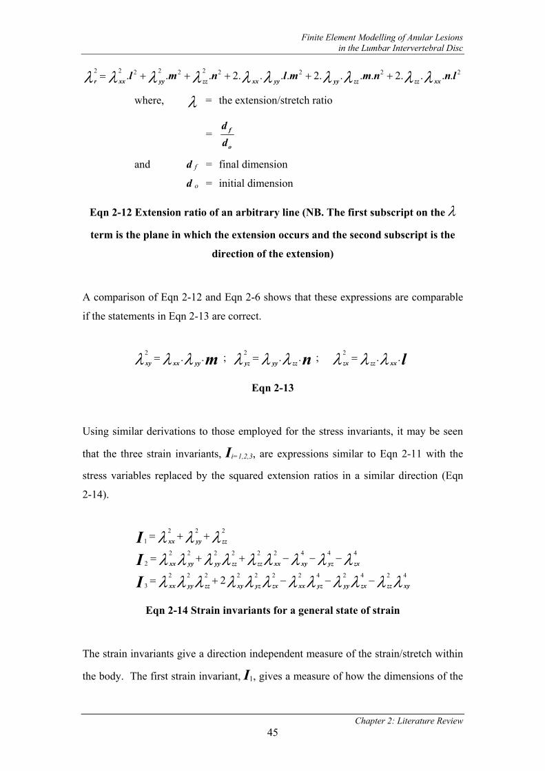
Finite Element Modelling of Anular Lesions in the Lumbar Intervertebral Disc
Chapter 2: Literature Review 45
2222222222 ....2....2....2... lnnmmlnml xxzzzzyyyyxxzzyyxxr λλλλλλλλλλ +++++=
where, λ = the extension/stretch ratio
= o
f
dd
and d f = final dimension
d o = initial dimension
Eqn 2-12 Extension ratio of an arbitrary line (NB. The first subscript on the λ
term is the plane in which the extension occurs and the second subscript is the
direction of the extension)
A comparison of Eqn 2-12 and Eqn 2-6 shows that these expressions are comparable
if the statements in Eqn 2-13 are correct.
myyxxxy ..2 λλλ = ; nzzyyyz ..2 λλλ = ; lxxzzzx ..2 λλλ =
Eqn 2-13
Using similar derivations to those employed for the stress invariants, it may be seen
that the three strain invariants, Ii=1,2,3, are expressions similar to Eqn 2-11 with the
stress variables replaced by the squared extension ratios in a similar direction (Eqn
2-14).
λλλλλλλλλλλλλλλλλλλλλ
λλλ
4242422222223
4442222222
2221
2 xyzzzxyyyzxxzxyzxyzzyyxx
zxyzxyxxzzzzyyyyxx
zzyyxx
III
−−−+=
−−−++=
++=
Eqn 2-14 Strain invariants for a general state of strain
The strain invariants give a direction independent measure of the strain/stretch within
the body. The first strain invariant, I1, gives a measure of how the dimensions of the

Finite Element Modelling of Anular Lesions in the Lumbar Intervertebral Disc
Chapter 2: Literature Review 46
body change. The second strain invariant, I2, is a measure of how the overall area of
the element changes and the third strain invariant, I3, indicates how the volume of the
body has changed.
2.7.1.2 Stress components and the strain energy equation, W (Reference:
Williams, 1973, Chapter 1; Ugural and Fenster, 1995)
Strain energy in a body will be independent of the orientation of the structure.
Therefore in finding an expression for strain energy, it is desirable to express this
quantity in terms of strain parameters which have no dependence on the body’s
orientation. Accordingly, the strain energy may be expressed as a function of the
strain invariants (Eqn 2-15).
( )IIIfW 321 ,,=
where, W = strain energy equation
Eqn 2-15 The general form of the strain energy equation
1
1
σ2
σ3
λ3
1 λ2
λ1
1
2
3
Undeformed
Deformed
σ1
Figure 2-10 Cube of unit length subjected to pure deformation to give side lengths of λ1, λ2 and λ3.

Finite Element Modelling of Anular Lesions in the Lumbar Intervertebral Disc
Chapter 2: Literature Review 47
Consider the application of a stress to a unit cube such that the final structure
experiences pure deformation and no shear. This deformation results in final edge
lengths of λ1, λ2 and λ3. Because there is no shear, these edge lengths are the
principal extensions. For this deformation, the strain invariants will not include any
terms for shear (Eqn 2-16).
λλλλλλλλλ
λλλ
2223
2222222
2221
..
...
zzyyxx
xxzzzzyyyyxx
zzyyxx
III
=
++=
++=
Eqn 2-16 Strain invariants for a body subjected to pure deformation
The force acting in direction 1 in Figure 2-10, F1, is defined in Eqn 2-17 in terms of
the stress acting in this direction, σ 1 and the area of the face on which this stress acts.
λλσ 3211 ..=F
Eqn 2-17
The displacement caused by this force, F1 is d λ1. Work is performed when a force
acts over some displacement, therefore, it may be seen that the above force, F1, does
work (Eqn 2-18).
λλλσ 13211 ... dW =
Eqn 2-18 Work performed by force, F1
An expression for a small change in the energy of the complete structure will include
the effects of the strain energies, Wi, due to the stresses applied in the 3 principal
directions (Eqn 2-19).

Finite Element Modelling of Anular Lesions in the Lumbar Intervertebral Disc
Chapter 2: Literature Review 48
λλλσλλλσλλλσ 321323121321 ......... ddddW ++=
Eqn 2-19 Expression for a small change in the stored energy in the structure
In order to determine a stress component such as σ1, equation Eqn 2-18 may be
rearranged to give Eqn 2-20.
λλλσ132
1 ..1
∂∂
=W
Eqn 2-20
Given that the strain energy equation for a material is a function of the three strain
invariants, Ii=1,2,3, (Eqn 2-15) the expression in Eqn 2-20 may be determined by
finding an expression for the partial derivative (Eqn 2-21).
λλλλ 3
3
32
2
21
1
11
...∂
∂
∂∂
+∂
∂
∂∂
+∂
∂
∂∂
=∂∂ I
II
II
IWWWW
Eqn 2-21
Substituting Eqn 2-21 and Eqn 2-16 into Eqn 2-20 results in an expression for the
stress in a compressible, isotropic structure that is subjected to a pure deformation
(Eqn 2-22).
∂∂
+∂∂
+∂∂
−∂∂
=IIIII
III
WWWW
33
22
22
1
3
1
2
15.03
1 .....2
λλσ
Eqn 2-22 Expression for a component of stress in a compressible, isotropic
material
The partial derivatives in Eqn 2-22 are the elastic property functions for the material.
Given the above expression for the state of stress in a compressible material, it is now
relevant to find a similar expression for the state of stress in an incompressible

Finite Element Modelling of Anular Lesions in the Lumbar Intervertebral Disc
Chapter 2: Literature Review 49
material. In order to do this, it is necessary to consider the effect a hydrostatic
pressure will have on the material. Since incompressible materials do not generate a
change in volume under load, the 3rd strain invariant, I3, will be equivalent to 1 (Eqn
2-16). Expressions for the strain invariants for incompressible materials may be
generated using the unity of I3 (Eqn 2-23).
1
111
3
2
3
2
2
2
12
2
3
2
2
2
11
=
++=
++=
I
II
λλλ
λλλ
Eqn 2-23 Strain invariants for an incompressible material
where the variables λ1, λ2 and λ3 are the principal extension ratios.
Hydrostatic stresses will result in no change in the strain energy. This may be seen by
manipulation of Eqn 2-19 when the stress components are set to σH and the
relationship λ1 . λ2 . λ3 = 1 is included. Therefore, the expression for the stress
components in an incompressible material will be similar to Eqn 2-20 with an
additional term for hydrostatic pressure (Eqn 2-24).
pW+
∂∂
=λλλσ
1321 .
.1 , where =p hydrostatic pressure
Eqn 2-24 Expression for stress in direction 1 in an incompressible material
If the hydrostatic pressure term was not included in Eqn 2-24, then it would not
accurately predict the stresses present when only a hydrostatic pressure was applied.
In this instance, the W∂ term would not predict any stress and the presence of the
hydrostatic pressure would not be evident.
On the basis of Eqn 2-24 expressions for the 3 stress components may be derived for
an incompressible material.

Finite Element Modelling of Anular Lesions in the Lumbar Intervertebral Disc
Chapter 2: Literature Review 50
pWW
pWW
pWW
II
II
II
+∂∂
−∂∂
=
+∂∂
−∂∂
=
+∂∂
−∂∂
=
22
31
2
33
22
21
2
22
22
11
2
11
.2..2
.2..2
.2..2
λλσλλσλλσ
Eqn 2-25 Stress components for an incompressible material
The strain energy equation, W , is a function of the strain invariants and satisfies the
condition that 0=W when, λ1 = λ2 = λ3 = 1.
2.7.2 Forms and Applications of the Strain Energy Equation
Mooney (1940) stated that the primary problem in elastic theory was to find a strain
energy equation which accurately described the material in question. He notes that if
the material is subjected to small strains and is isotropic and homogeneous, then an
expression for the strain energy of the material may be derived on the basis of the
elastic modulus and rigidity modulus. However in the case of rubber, the strains
observed are too large for the materials mechanical behaviour to be accurately
modelled using classic small strain theory. Mooney (1940) noted the necessity for the
development of a relationship which could suitably describe the nonlinear, elastic,
large strain behaviour of rubbers.
Mooney (1940) observed that under uniaxial loading, the mechanical response of
rubber is nonlinear, while under shear loading, the mechanical response follows
Hooke’s law. Also, rubbers behave as near incompressible materials. On the basis of
these criteria, Mooney (1940) developed two strain energy equations to describe
rubber mechanics. The first equation assumed that the material was linear in shear
and incompressible (Eqn 2-26) and the second equation assumed the material was
nonlinear in shear and incompressible. However, the second equation was later
discounted as incorrectly representing the behaviour of rubbers (Rivlin, 1984). An

Finite Element Modelling of Anular Lesions in the Lumbar Intervertebral Disc
Chapter 2: Literature Review 51
additional assumption associated with the Mooney equation that assumed linear shear
behaviour was that the material was isotropic.
)3111()3(),,( 2
3
2
2
2
12
2
3
2
2
2
11321 −+++−++=λλλλλλλλλ CCW
where, C1 and C2 are material constants
Eqn 2-26 Mooney Strain Energy Equation
The expression in Eqn 2-26 was later altered by Rivlin (1984) to incorporate the strain
invariants (Eqn 2-27).
λλλ 2
3
2
2
2
11 ++=I ; λλλ 2
3
2
2
2
12
111 ++=I ; λλλ 2
3
2
2
2
13 ..=I
Eqn 2-27 Strain Invariants
This equation was then referred to as the Mooney-Rivlin equation (Eqn 2-28) where
the expressions for I1 and I2 were substituted into Eqn 2-26. For incompressible
materials, I3 is equivalent to 1.
)()( 33 2211 −+−= ICICW
Eqn 2-28 Mooney-Rivlin strain energy equation
Several researchers have used hyperelastic material formulations to represent the
material behaviour of biological tissues.
The Mooney-Rivlin strain energy equation has been applied to nonlinear biological
tissues in previous studies (Crisp, J. D. C in Fung et al., 1972; Weiss et al., 2001;
Bilston et al., 2001; Vossoughi, 1995; George et al., 1988) as both a complete model
for the tissue and as a base model which was further developed to include
viscoelasticity or poroelasticity of the tissue. Natali and Meroi (1990) and Natali

Finite Element Modelling of Anular Lesions in the Lumbar Intervertebral Disc
Chapter 2: Literature Review 52
(1991) represented the behaviour of the nucleus pulposus and of the disc material in
general using a Mooney-Rivlin material description. However, it is considered that
the hyperelastic material law would be better applied to the behaviour of the anulus
fibrosus ground substance rather than the nucleus pulposus given the low shear
stiffness and semi-fluid nature of the nucleus pulposus.
Crisp (in Fung et al., 1972) states that the regular implementation of the Mooney
strain energy equation was due to its simplicity – most other strain energy equations
hitherto developed were quite complex and not readily comprehended by researchers
unfamiliar with the mathematics that forms their basis. An additional attraction
offered by the Mooney-Rivlin equation was the ease with which the constants could
be determined from experimental data – these constants were the gradient and
intercept of the best fit curve. The Mooney-Rivlin equation may have provided an
adequate fit for experimental data at very low strains, but at high strains, the
inaccuracy in the model became apparent (Crisp in Fung et al., 1972).
One of the integral assumptions made in the derivation of the Mooney-Rivlin equation
was the linear relationship between the shear stress and the shear strain. The results
from experimental testing on the anulus fibrosus ground substance (Chapter 4)
suggested that this material was in fact nonlinear under shear loading. Similar
observations may be made for other biological tissues (Yamada, 1970).
There are a considerable number of hyperelastic strain energy equations which have
been developed to incorporate nonlinear shear behaviour as well as more complex
behaviour such as viscoelasticity, poroelasticity or anisotropy.
Tschoegl (1971) extended the Mooney-Rivlin strain energy equation to include higher
orders of the strain invariants and to represent nonlinear shear behaviour. The general
form of these polynomial models is expressed in Eqn 2-29. It was observed that these
higher order combinations provided a more accurate representation of the
experimental results, in particular at high strains.

Finite Element Modelling of Anular Lesions in the Lumbar Intervertebral Disc
Chapter 2: Literature Review 53
jiN
jiij IICW )3()3( 21
1
−−= ∑=+
where, Cij are material constants
Eqn 2-29 General form of the polynomial strain energy equations
Ogden (1972) developed a strain energy equation which involved the assumption of
nonlinearity of the material response under shear loading (Eqn 2-30).
)3.(.2321
12 −++= −−−
=∑ iii
N
i i
iW ααα λλλαµ
where, µi and αi are material constants
Eqn 2-30 The Ogden strain energy equation
The Ogden strain energy equation (Eqn 2-30) has been applied to both mechanical
engineering situations (Andra et al. 2000; Jemiolo and Turteltaub 2000; Salomon et
al. 1999) and to simulate biological tissues (Miller and Chenzei, 2002; Jemiolo and
Telega, 2001; Zobitz et al., 2001; Tang et al. 1999).
Other researchers have proposed strain energy equations to describe biological
tissues. Bischoff et al. (2002) developed a strain energy equation which incorporated
orthotropy to represent the mechanical contribution of the fibres in soft tissues. Weiss
et al. (2001) modelled the mechanical behaviour of ligaments and due to the
difficulties encountered in fitting the nonlinear shear response of the ligaments with
the Mooney-Rivlin equation they implemented a strain energy equation that modelled
the material as a fibre reinforced composite (Veronda and Westmann, 1970). A more
complex model was proposed by Rubin and Bodner (2002) which incorporated both
an elastic component and a dissipative component. The elastic component accounted
for the anisotropy of the fibres and for dilation and distortion in the material. The
model also accounted for the recovery of the deformed shape with time. Criscione et
al. (2000) developed a strain energy equation to model isotropy in a finitely
deforming material.

Finite Element Modelling of Anular Lesions in the Lumbar Intervertebral Disc
Chapter 2: Literature Review 54
2.8 Experimental Testing of the Intervertebral Disc
Details of relevant previous studies that have involved experimental testing of the
intervertebral disc are outlined in the following section. The literature was reviewed
to obtain information on the mechanical behaviour of the anulus fibrosus in terms of
its constituents (i.e. the collagen fibres and the ground substance).
2.8.1 Types of Testing Carried out and Material Information Available in
Literature
Experimental testing of the intervertebral disc has been carried out to determine the
behaviour of either the disc as a complete entity or to quantify the behaviour of the
individual components, specifically the anulus fibrosus. Testing on the anulus
fibrosus was for the purpose of determining the overall response of the tissue rather
than for quantification of the response of the individual materials from which it is
comprised.
Researchers have carried out static loading, impact loading, relaxation and vibrational
testing on isolated cadaveric intervertebral discs in order to quantify the mechanical
properties of the structure (Brown et al., 1957; Hirsch, 1955; Virgin, 1951).
Testing has been carried out on specimens of anulus fibrosus under various loading
conditions. Acaroglu et al. (1995), Skaggs et al. (1994), Fujita et al. (1997) and Wu
and Yao (1976) carried out tensile testing on dumb-bell or rectangular shaped
specimens of anulus fibrosus. The specimens used by Acaroglu et al. (1995), Skaggs
et al. (1994) and Fujita et al. (1997) were region specific. This allowed for details of
the inhomogeneous tensile response of the anulus fibrosus to be quantified. Evidence
was provided for this inhomogeneity of the anulus in both a radial and circumferential
direction. Acaroglu et al. (1995) carried out this testing on both healthy and
degenerate specimens in order to evaluate the effects of aging on the tensile properties
of the tissue.

Finite Element Modelling of Anular Lesions in the Lumbar Intervertebral Disc
Chapter 2: Literature Review 55
Best et al. (1994) carried out experiments on plugs of anulus fibrosus from the
anterior and posterolateral anulus fibrosus to determine the swelling response and the
compressive creep response. The orientation of these specimens was such that the
compressive load was applied in a radial direction to cylinders with a 5mm diameter.
This research provided data on the hydraulic permeability of the anulus and the elastic
modulus of the anulus fibrosus solid matrix (ie. all structures of the anulus fibrosus
except the water and electrolytes). Best et al. (1994) found evidence for the
inhomogeneity of the anulus fibrosus both radially and circumferentially.
Iatridis et al. (1999) demonstrated the shear response of the anulus fibrosus by testing
cylindrical specimens under torsional loading at various amplitudes and frequencies.
Fujita et al. (2000) also carried out shear testing on specimens of anulus fibrosus with
various orientations. The stress-strain results from these tests were not published and
only values of the shear modulus were stated. They found the shear modulus in the
outer anulus was 3-5 times larger than the inner anulus.
There was no evidence found in the literature for experimentation that has been
carried out to determine the mechanical behaviour of the anulus fibrosus ground
substance. All previous researchers aimed to quantify the response of the composite
tissue. Additionally, there was no evidence for the mechanical response of the tissue
under biaxial compression.
2.8.2 Specimen Handling
The details of techniques used to maintain fluid content in disc material and the
freezing temperatures employed are listed in Table 2-6.

Finite Element Modelling of Anular Lesions in the Lumbar Intervertebral Disc
Chapter 2: Literature Review 56
Table 2-6 Details of specimen handling techniques employed by previous
researchers
Adams et al.
(1994)
- Spinal specimens were placed in a sealed plastic bag and frozen
at -17oC.
- On the day of dissection the spines were thawed at 3oCfor 12
hours
- The discs were generally tested on the same day and if not were
stored overnight for testing the next day. The specimens were
stored in a vacuum sealed bag
- While the specimens were tested they were protected from fluid
loss by a polythene film
Pearcy and
Hindle (1991)
- Spinal specimens were stored at -20oC until they were to be
dissected
- For dissection the specimens were thawed and the fat and
muscles were removed
- The soft tissue was kept moist during the dissection and testing
using Ringers solution
Ebara et al.
(1996)
- Lumbar spines were stored in a sealed plastic bag and frozen at
-20oC
- For dissection the spines were partially thawed, the disc removed
and cut in half and then these specimens refrozen in double-
sealed plastic bags at -20oC until the day of testing
- Ebara et al. (1996) carried out a pilot study to determine the
most effective environmental condition for the specimens and
determined that immersion in 0.15M saline solution for 15
minutes brought the hydration of the tissue to 96% of the final
equilibrium value
- On the day of testing the frozen disc portion was sectioned into
blocks of anulus. These blocks of anulus were still frozen and
were sectioned into smaller portions, soaked in saline solution
for 15 minutes to equilibrate and then sectioned into test
specimens

Finite Element Modelling of Anular Lesions in the Lumbar Intervertebral Disc
Chapter 2: Literature Review 57
Iatridis et al.
(1999)
- The spines were sealed in plastic and frozen at -20oC
- The intervertebral discs were removed from the thawed spines
and the discs refrozen at -80oC
- On the day of testing blocks were removed from the anulus,
mounted on a freezing stage and test specimens cut from these
blocks
- Specimens were frozen or wrapped in plastic during all
preparation steps to maintain the hydration level
- The specimens were tested in an environmental chamber filled
with 0.15M saline solution
Best et al.
(1994)
- These researchers attempted to employ a technique which
limited dehydration and proteoglycan leaching
- Intact motion segments were frozen at -20oC
- The intervertebral discs were dissected from the spine in a
humidity chamber which was maintained at room temperature
and > 95% R.H.. The discs were then refrozen at -80oC
- Blocks were cut from the frozen discs
- The blocks were frozen onto a stage at -20oC and remained
frozen while the test pieces were removed
- The test specimens were stored frozen at -80oC until the day of
testing
Skaggs et al.
(1994)
- On the day of dissection the lumbar spines were cut mid-
sagittally, sealed in plastic and frozen at -20oC until the day of
testing
- On the day of testing the hemidiscs were thawed and the disc cut
from the bone. During this procedure the tissue was kept moist
with saline soaked gauze
- The specimens were tested immersed in 0.15 M saline solution
Markolf and
Morris (1974)
- The intervertebral discs were removed at autopsy and tested soon
afterward
- The discs were kept moist during testing using saline solution

Finite Element Modelling of Anular Lesions in the Lumbar Intervertebral Disc
Chapter 2: Literature Review 58
From Table 2-6 it appears that common practice for specimen handling when testing
intervertebral discs and in particular the anulus fibrosus involves freezing of the entire
spine at -20oC until the dissection of the disc or specimens is to take place. The
spines are commonly wrapped in plastic to avoid fluid loss and when thawing is
desirable, this is done gradually. However, the test specimens are generally sectioned
from the discs or spine while they are frozen in order to avoid unnecessary fluid loss.
During the sectioning procedure, the tissue fluid level is maintained using Ringers
solution or saline solution, either by wrapping the specimen in fluid soaked gauze or
by applying the solution directly.
2.9 Conclusions
From the review of literature it was concluded that an investigation into the
biomechanical effects of anular lesions on the disc mechanics would provide valuable
information. This information would serve to improve the current state of
understanding of the mechanisms for degeneration of the intervertebral disc and the
necessity and suitability of current techniques for treatment of back pain.
In order to carry out this investigation a finite element model of the intervertebral disc
was proposed. This technique for developing a computational model of a mechanical
structure provides a unique method for determination of both the external and internal
stress state present within the materials that comprise the structure. Determination of
the internal stress state of the intervertebral disc components in a model of both a non-
degenerate and a degenerate disc would provide useful information on the change in
stiffness and deformation in the disc as a result of anular lesions. Representation of
the individual components of the intervertebral disc, in particular the anulus fibrosus
ground substance and the collagen fibres would provide a broader description of the
loaded stress state in the intervertebral disc.
Representation of the anulus ground substance using a hyperelastic material
formulation would provide a close representation for the highly nonlinear behaviour
of the material. Additionally, it was desirable to simulate the condition of the
intervertebral disc at strain rates simulating common physiological loading conditions,

Finite Element Modelling of Anular Lesions in the Lumbar Intervertebral Disc
Chapter 2: Literature Review 59
therefore, the assumption of incompressibility inherent in the hyperelastic material
laws was ideal. Initially, a Mooney-Rivlin strain energy equation was used to
represent the ground substance. Even though it was stated that this material
formulation involved an assumption of linearity during shear loading, several
previous researchers had used this equation to represent biological tissues and the
determination of material parameters was relatively straight-forward.
A preliminary finite element model of the intervertebral disc was developed. This
model was used to determine the suitability of the material formulations and
parameters employed to describe the disc components and to refine the loading
conditions applied to the model to simulate the physiological condition. Details of
development and analysis of this model are the subject of Chapter 3.

Finite Element Analysis of Anular Lesions in the Lumbar Intervertebral Disc
Chapter 3: Development of the Preliminary FEM 60
CChhaapptteerr
33
DDeevveellooppmmeenntt ooff tthhee PPrreelliimmiinnaarryy
FFEEMM
The review of previous studies that have analysed the biomechanics of the
intervertebral disc suggested that the use of the finite element method was the most
appropriate means to analyse the effects of anulus lesions on the disc mechanics.
Several of the finite element models developed by previous researchers to investigate
loading on the intervertebral disc included the adjacent vertebrae, the posterior
elements and/or some spinal muscles. Since the primary structure of interest in the
current study was the intervertebral disc, it was decided that simulation of the
structures external to the disc using specific loading and boundary conditions would
permit a more computationally efficient analysis to be performed. It was desirable to
obtain an extremely detailed and accurate finite element model of the intervertebral
disc in order to better understand the effects of lesions on this structure.
Chapter 3 details the development and analysis of a preliminary finite element model.
The finite element model consisted of the anulus fibrosus, the cartilaginous endplates
and the nucleus pulposus. There was no bony anatomy, musculature or ligaments
included in the model. The majority of the details of this model were maintained in
the FEM which was developed for the final analyses (chapter 8 and 9). Development
of the preliminary model was carried out to determine the acceptability of the
modelling methodology employed for the components of the disc.

Finite Element Analysis of Anular Lesions in the Lumbar Intervertebral Disc
Chapter 3: Development of the Preliminary FEM 61
3.1 Basic description of the FE method
The finite element method was described by Zienkiewicz (1980). This method
involves the subdivision of a continuous structure into finite regions. These regions
are in 1, 2 or 3 dimensional space and are referred to as elements. The finite elements
are connected by common points called nodes. When all these regions are connected
the resulting arrangement is referred to as a mesh.
Degrees of freedom exist at the nodes and are mutually independent variables of
displacement and/or rotation which define the node’s position and orientation in
space. For a mechanical system a relationship exists between the displacement and
the force at the nodes (Eqn 3-1).
uKf .=
where, f = externally applied force and moments
u = displacements and rotations
K = the stiffness of the system
Eqn 3-1 Force-displacement equation
In a linear system the stiffness is calculated directly from the geometry of the
structure and the elastic stiffness characteristics of the material. For nonlinear
systems, constants describing the mechanical behaviour at each node are collated into
a system of equations for the entire structure and this is expressed in matrix form
as K , the stiffness matrix. This matrix is dependent on the material properties and on
the geometry of the structures being modelled.
Basic features of any structure analysed using the finite element method are the
boundary and loading conditions. These conditions are in the form of forces/moments
and displacements/rotations. Forces and moments applied to the nodes of the model
are defined in the matrix f and any known displacements and rotations are defined in
the matrix, u .

Finite Element Analysis of Anular Lesions in the Lumbar Intervertebral Disc
Chapter 3: Development of the Preliminary FEM 62
The combined finite element mesh, loading and boundary conditions and material
relationships for the structure are collectively called the finite element model, FEM.
Once the finite elements have been generated, common nodes between them
prescribed and the boundary and loading conditions entered, it is possible to solve the
system of equations governing the mechanical response of the structure to find the
unknown values of displacements.
fKu .1−=
Eqn 3-2 The displacements are determined using the inverse of the stiffness
matrix.
For a nonlinear FEM, this is achieved by matrix manipulation to determine the inverse
of the stiffness matrix. It is an iterative procedure requiring complex matrix algebra.
Analysis of linear systems requires the direct solution of equation Eqn 3-2 since the
stiffness of the system can generally be calculated directly.
An advantage of the finite element method is that it can be enlisted to solve problems
of fluid dynamics or mechanics that involve complicated or geometrically nonlinear
structures. Irrespective of geometry, these structures may be subdivided into elements
to create a mesh and a solution obtained. The only limit on the structures and systems
which can be solved using the finite element method is the processing power available
to solve the complex iterative algorithms involved in this method.
Whilst all aspects of the finite element model control the final accuracy of the
solution, an integral component of the FEM is the relationship that is prescribed
between the displacement and the force at the nodes in the mesh. Inaccuracy in the
material properties for the model components can have drastic effects on the results of
the model and it is essential that the material properties prescribed for the FEM
components mimic the realistic response of the structures.

Finite Element Analysis of Anular Lesions in the Lumbar Intervertebral Disc
Chapter 3: Development of the Preliminary FEM 63
Commercial software packages are available which facilitate the development and
solution of finite element problems. Examples of these packages are HKS Abaqus
(Worley Advanced Analysis) and ANSYS (Leap Australia Pty Ltd).
3.2 Abaqus 6.3 Finite Element Modelling Software
Commercially available finite element software, Abaqus/Standard 6.3 was used for
the generation of the finite element model. The Abaqus finite element products were
originally developed in the USA by David Hibbitt, Bengt Karlsson and Paul Sorenson
as a tool for structural analysis in engineering applications. This package was
employed as it was robust modelling software, which had experienced widespread use
in both mechanical and biomechanical applications. Additionally, Abaqus was well
suited to the analyses of the intervertebral disc which were static problems involving
nonlinear material properties and nonlinear geometry.
Abaqus 6.3 provided an extensive suite of material descriptions including the
hyperelastic material model employed for the development of the intervertebral disc.
The software was capable of modelling this tissue using a variety of classic models
such as the Mooney equation (Mooney, 1940) and the Ogden model (Ogden, 1972) as
well as providing for a user defined material description. If the material constants for
the model were known, they could be input directly. However, if the material being
modelled did not have documented material constants the user could input raw test
data from specific experimental testing on material samples and Abaqus 6.3
calculated the necessary constants using a least squared error algorithm (Abaqus
Theory Manual, § 4.6.2).
The Abaqus 6.3 software incorporated user-friendly preprocessor input commands
and postprocessing facilities. There was an extensive element library and methods
available for nodal and element constraints were well suited to the current application.

Finite Element Analysis of Anular Lesions in the Lumbar Intervertebral Disc
Chapter 3: Development of the Preliminary FEM 64
3.2.1 Specifics of finite element analysis carried out using Abaqus 6.3
The FEM could be generated using the graphic user interface, Abaqus/CAE or using a
data file containing the necessary information on the model geometry, mesh, material
properties and the boundary and loading conditions. The latter option was employed
for the development of the FEM as it allowed for greater control over the form of the
mesh which was generated and the model details prescribed. With the use of the data
file, or input file, it was possible to generate finite element models of varied mesh
density and mechanical properties.
Abaqus organised the input of the boundary and loading conditions into specific
analysis phases called steps. The loading that was being simulated was organised into
specific events which were then analysed successively by the software as individual
steps. Each step was associated with a time frame. By default the time for any given
step was 1.
For nonlinear analyses such as the intervertebral disc FEM, the steps were subdivided
into increments. An increment corresponded to the application of a portion of the
total load and boundary condition for a particular step. The length of the increment
was dependent on the time frame over which the step occurred and on convergence
difficulties encountered by the software. If the time frame for the increment was too
long, then the change in the displacement and force condition over this time would be
too large and Abaqus may not have been able to converge on a solution for that
period. In this instance, the software automatically reduced the time period for that
increment – perform a time-cutback - and attempted to resolve. Abaqus would only
carry out time-cutbacks 5 times. If any more attempts were required the software
considered that the solution was diverging and a valid solution could not be obtained.
If the time period for the increment was too small, Abaqus would carry out
unnecessary calculations and thus inefficiently use processing time. In order for a
timely solution to be obtained, the user could designate a minimum and maximum
time period for the increments and Abaqus attempted to find a solution within this
range.

Finite Element Analysis of Anular Lesions in the Lumbar Intervertebral Disc
Chapter 3: Development of the Preliminary FEM 65
In order to determine whether a FEM analysis was converging on a solution in any
given increment, Abaqus analysed the residuals of the fluxes and the corrections to
the displacements. Both the residuals and the corrections were errors in the
force/displacement or moment/rotation equations. The residuals related to errors in
the fluxes – force and moments – and the corrections related to errors in the nodal
variables – displacement and rotation.
If the largest residual force or moment was more than 0.5% of the time average force
or moment, then Abaqus did not consider that equilibrium had been achieved for that
variable and would initiate further iteration. If the largest correction to any nodal
variable was greater than 1% of the largest change in the nodal variable then the
equilibrium of that variable was not achieved. Abaqus would provide information on
the nodes at which the residuals or corrections were too large and the associated
degree of freedom (Table 3-1).
Table 3-1 Abaqus output for convergence of analysis increments
Abaqus required that the residuals or corrections in each iteration of a step, converge
quadratically in accordance with the Newton-Raphson criteria. If they did not
decrease in accordance with this criterion Abaqus warned that the solution was either
converging too slowly or diverging.
EQUILIBRIUM ITERATION 1 AVERAGE FORCE 2.32 LARGEST RESIDUAL FORCE -3.207E-02 AT NODE 165510 DOF 2 LARGEST INCREMENT OF DISP. -3.825E-03 AT NODE 119570 DOF 2 LARGEST CORRECTION TO DISP. -1.179E-02 AT NODE 119570 DOF 2 FORCE EQUILIBRIUM NOT ACHIEVED WITHIN TOLERANCE AVERAGE MOMENT 0.00 LARGEST RESIDUAL MOMENT -8.656E-04 AT NODE 9999999 DOF 6 LARGEST INCREMENT OF ROT’N -2.201E-07 AT NODE 10 DOF 4 LARGEST CORRECTION TO ROT’N -3.246E-08 AT NODE 10 DOF 6 THE MOMENT IS ZERO EVERYWHERE BUT THE MOMENT RESIDUAL OR THE ROTATION CORRECTION IS NON-ZERO AVERAGE CAV. VOL. 1.97 LARGEST RESIDUAL CAV. VOL. 1.473E-05 AT NODE 2 DOF 8 LARGEST INCREMENT OF H. PRESS. 1.513E-05 AT NODE 2 DOF 8 LARGEST CORRECTION TO H. PRESS. -1.984E-05 AT NODE 2 DOF 8 H PRESS. CORRECTION TOO LARGE COMPARED TO H. PRESS. INCREMENT EQUILIBRIUM ITERATION 2 …

Finite Element Analysis of Anular Lesions in the Lumbar Intervertebral Disc
Chapter 3: Development of the Preliminary FEM 66
3.3 Geometry of the Anulus Fibrosus and Nucleus Pulposus in the Transverse
Plane
The spinal level modelled was the L4/5 lumbar level. This decision was based on
reports from clinicians of the prevalence of anulus lesions in this level of the spine.
The finite element model developed consisted of only the L4/5 intervertebral disc.
There was no musculature, ligaments or bony attachments. The actions of these
structures were simulated through the boundary and loading conditions applied to the
model.
In order to develop a dimensionally accurate FE model of the disc, it was necessary to
accurately represent the outer disc profile. Existing literature in the area provided
only gross dimensions for the full anterior-posterior depth and for the lateral width.
There was very little information available on the precise curvatures and form of the
outer anulus and nucleus transverse boundaries. This was largely due to the
significant variation in these dimensions between different specimens.
One approach to obtaining the necessary dimensions would have been to measure the
dimensions from a series of specimens and attempt to develop a standard dimensional
data series for the different sections of the disc. However, this would have proven to
be time consuming and more importantly, due to the high degree of variation in the
shape and area of different discs from the same level of the spine, it may have been
prone to a high level of error.
Alternatively, the approach adopted was to develop a series of formulae to
appropriately represent the anulus and nucleus boundaries. These formulae would be
applied on the basis of a sequence of twelve significant points on the outer boundaries
and could be manipulated to represent any disc shape.
The co-ordinates of the boundary nodal points were defined using the formulae. To
make the identification and input of the nodal points more straight-forward, it was
desirable for them to be input directly into the FE input file using Matlab execution
codes.

Finite Element Analysis of Anular Lesions in the Lumbar Intervertebral Disc
Chapter 3: Development of the Preliminary FEM 67
The formulae were developed using data from the images obtained by Vernon-
Roberts et al. (1997) for the L4/5 lumbar intervertebral discs (Figure 3-1).
Additionally, other morphological data from this study was used for validation of the
final formulae.
Figure 3-1 Picture of a sectioned cadaveric intervertebral disc.
3.3.1 Methods – anulus boundary
The following section details the development of formulae to map the outer boundary
of the anulus fibrosus and the criteria used to determine the accuracy of these
formulae.
3.3.1.1 Measurements
Photographs of sectioned intervertebral discs were used to obtain tracings of the outer
anulus boundaries in the L4/5 disc of 18 specimens from various age groups.
In order to define the regions, over which each formula was to apply, the disc was
divided into 6 separate sectors. These sectors were defined using 4 tangent lines and
6 intersection points on the anulus boundary.
The lines and points were defined as shown in (Figure 3-2 and Figure 3-3).

Finite Element Analysis of Anular Lesions in the Lumbar Intervertebral Disc
Chapter 3: Development of the Preliminary FEM 68
• Points 5 and 1 – the 2 intersections of a line (line A) drawn tangent to the most
posterior points on the anulus boundary
• Points 2 and 4 – defined by the intersection of 2 lines drawn perpendicular to line
A (called lines B and D, respectively) and tangent to the lateral-most points
• Point 3 – defined by a line (line C) parallel to A and intersecting the most anterior
point
• Point 0 – intersection of a line (line E) parallel to line A and intersecting the most
anterior point in the posterior concavity of the disc
Figure 3-2 Tangent lines creating the rectangular boundary in the transverse
sectioned view of a disc
Radial lines from the geometric centre to these points were denoted r0, r1, …, r6. The
lengths of these radii and the angle (θ) from the x axis to the radii were measured
(Figure 3-3).
The disc centre was the geometric centre of a rectangle, defined by lines A through D.
The rectangular co-ordinate axes were defined in relation to lines A and B with the x
axis passing through the geometric centre, parallel to line B and the y axis through the

Finite Element Analysis of Anular Lesions in the Lumbar Intervertebral Disc
Chapter 3: Development of the Preliminary FEM 69
centre, parallel to line A – so orientating the disc with its left lateral side down (Figure
3-3).
Figure 3-3 Definition of anulus boundary points
3.3.1.2 Development of equations
Each point on the anulus boundary was defined using parametric equations and the
basic form of the equations for sectors 1 to 4 was an ellipse (Eqn 3-3).
θθ
coscos
y
x
ryrx
==
Eqn 3-3 Parametric equations for an ellipse
The typical form for the equations developed is shown in Eqn 3-4.

Finite Element Analysis of Anular Lesions in the Lumbar Intervertebral Disc
Chapter 3: Development of the Preliminary FEM 70
).sinsin().()(
).coscos().()(
PcurveofperiodnecessaryangleinitialradiisuccessiveofvaluesyindifferenceyofvalueinitialY
PcurveofperiodnecessaryangleinitialradiisuccessiveofvaluesxindifferencexofvalueinitialX
++=
++=
radiiboundingthebetweenrotationangulartotalradiifirstfromrotationangularP =
Eqn 3-4 Typical form for the equations to plot sectors 1 to 4
The value of θ was increased through each sector to generate the series of bounding
points.
A cosine or a sine term could be applied because for a specific angular period, the y
variation of these terms was similar to the variation of the difference between the radii
in any given segment. Since the points 0 to 5 were located at the tangent points to
perpendicular lines, the gradients at each point were readily defined as zero or
infinity. If Eqn 3-4 was applied piecewise to each sector, then the gradients at the
ends of each of these sectors could be manipulated to ensure continuity. This was
achieved by selecting the ‘necessary period of the sine and cosine curves’ to be
continuous between each sector. This was shown in the choice of the period for the
curves in Eqn 3-5.
The parametric equations used to represent each sector were:
Sector 1
( )
( )
−−
−+=
−−
−+=
12
1112211
12
1221122
.2
sin.sin.sin.sin.
.2
cos.cos.cos.cos.
θθθθπθθθ
θθθθπθθθ
rrry
rrrx for 21 θθθ <<
Sector 2
( )
( )
−−
+−+=
−−
+−+=
23
2332233
23
2332222
.22
sin.sin.sin.sin.
.22
cos.cos.cos.cos.
θθθθππθθθ
θθθθππθθθ
rrry
rrrx for 32 θθθ <<

Finite Element Analysis of Anular Lesions in the Lumbar Intervertebral Disc
Chapter 3: Development of the Preliminary FEM 71
Sector 3
( )
( )
−−
+−+=
−−
+−+=
34
3443333
34
3334444
.2
sin.sin.sin.sin.
.2
cos.cos.cos.cos.
θθθθππθθθ
θθθθππθθθ
rrry
rrrx for 43 θθθ <<
Sector 4
( )
( )
−−
+−−=
−−
+−+=
45
4554455
45
4445544
.22
3sin.sin.sin.sin.
.22
3cos.cos.cos.cos.
θθθθππθθθ
θθθθππθθθ
rrry
rrrx for 54 θθθ <<
Eqn 3-5 Parametric equations to plot sectors 1 to 4
The choice of the ‘initial angle’ and the ‘necessary period of the curve’ for each sector
were dependent upon whether the x and y co-ordinates were increasing or decreasing
over the sector. For example, in sector 4 it may be seen from Figure 3-3 that the x co-
ordinate will increase over the trajectory from r3 to r4 and the y co-ordinate will
decrease over the trajectory from r3 to r4. Figure 3-4 shows that the region on both the
cosine and sine curves where this occurred was from π to 23π . Hence the initial
angle was π and the period of the curve was 2π . In this way the x co-ordinate
varied from 33 cos. θr to 44 cos. θr and the y co-ordinate will vary from 33 sin. θr to
44 sin. θr .
-1.5
-1
-0.5
0
0.5
1
1.5
0 3.14159 6.28318Angley
cos(θ) sin(θ)
Figure 3-4 Cosine and sine curve showing angle over which the parametric equations are chosen

Finite Element Analysis of Anular Lesions in the Lumbar Intervertebral Disc
Chapter 3: Development of the Preliminary FEM 72
The form of the equations for sectors 0 and 5 varied from the other sectors, due to the
inflection point present on their boundaries. An attempt was made to fit a cosine or
an arcsine equation for these sectors, but the inflection points produced with these
were too severe resulting in an inaccurate and exaggerated representation of the
posterior concavity. Instead, a cubic equation was used for these segments.
The general forms of the 4 constants for the cubic equation (Eqn 3-6) were
determined using the commercial mathematical program, Maple V. These are
detailed in Eqn 3-7.
dcxbxaxy +++= 23
Eqn 3-6 Cubic equation
3223
2323
..3..3
...3....3.
.).(.6
)(.2
)).((.3
llnlnnKK
lnmnmonlold
Knlomc
Komb
Klnoma
−+−=
−++−=
−=
−=
+−−=
where, l = x co-ordinate of first point in sector path
m = y co-ordinate of first point in sector path
n = x co-ordinate of second point in sector path
o = y co-ordinate of second point in sector path
Eqn 3-7 Defining constants for the cubic equations modelling sectors 0 and 5
All the sector equations were implemented using Matlab code and a separate file
developed containing the data values for the radii and associated angles for each
specimen (Appendix A).

Finite Element Analysis of Anular Lesions in the Lumbar Intervertebral Disc
Chapter 3: Development of the Preliminary FEM 73
3.3.1.3 Disc area
For the purposes of validation of the formulae, it was necessary to develop a method
for determining the area of all the sectors of the entire disc surface.
This was achieved by using numerical integration. Traditional methods of numerical
integration such as Simpson's rule or the Trapezium rule could not be applied as this
was a finite area within a distinct outer boundary rather than a curve on the two
dimensional plane. Therefore, a method involving the cumulative sum of the areas of
a series of triangles was used.
The two long sides of the triangle intersected at the geometric centre and the smaller
side was the distance between any two adjacent points on the outer boundary. A
Matlab code was developed to calculate the final sum (Appendix A).
3.3.1.4 Validation of the anulus formulae
Two criteria were used to validate the final formulae:
• Firstly, a visual validation was used. If the general shape of the disc matched
that of the original specimen, in terms of curvature, gradients and turning
points, then the formulae were considered to be suitable.
• Secondly, the area of the overall disc shape was determined. This area was
compared with the discal area data provided by the study carried out by
Vernon-Roberts et al. (1997).
In terms of the visual validation, the formulae developed produced plots with outer
boundaries very similar to the specimens from which they were taken. However, each
sector was slightly more curved outward than the original tracing of the disc. This
was due to the initial assumption that the sector formulae were of an elliptical form.
Even so, the discrepancy between the areas calculated during this study and those
provided by Vernon-Roberts et al. (1997) were relatively low (Figure 3-5 and Figure
3-6). Also, this error was generally negative, indicating that the areas calculated from

Finite Element Analysis of Anular Lesions in the Lumbar Intervertebral Disc
Chapter 3: Development of the Preliminary FEM 74
the formulae were conservative and that the over-representation of the curvature of
the boundary did not greatly impact on the final disc shape.
0
500
1000
1500
2000
2500
3000
8 12 16 29 33 37 38 39 40 41 43 44 45 48 50 56 57 58Specimen number
Are
a (m
m2)
Current study Vernon-Roberts et al. (1997) Figure 3-5 Comparison of total disc area with the results from Vernon-Roberts et
al. (1997)
-15
-10
-5
0
5
10
15
8 12 16 29 33 37 38 39 40 41 43 44 45 48 50 56 57 58
Specimen number
Perc
enta
ge
Percentage Variation
Figure 3-6 Percentage variation in disc area compared to the area values from Vernon-Roberts et al. (1997)
3.3.2 Methods – nucleus
This section details the development of formulae to map the outer profile of the
nucleus pulposus and the criteria used to validate this technique.

Finite Element Analysis of Anular Lesions in the Lumbar Intervertebral Disc
Chapter 3: Development of the Preliminary FEM 75
3.3.2.1 Measurement
Measurements taken for the nucleus boundary were similar to those obtained for the
anulus boundary. A local x-y co-ordinate system was constructed using the same
approach as was outlined for the anulus.
However, there were 3 additional dimensions obtained, which allowed the nucleus
location and orientation relative to the anulus to be defined. These additional
dimensions included:
• the radial distance from the geometric centre of the anulus to the geometric
centre of the nucleus;
• the angle from the x axis of the anulus to a line between the anulus geometric
centre and the nucleus geometric centre; and
• the angle between the x-axis of the anulus and the x-axis of the nucleus.
Fewer specimens were used to determine the formulae for the nucleus profile because
only specimens with a distinct boundary between the anulus and nucleus were chosen.
3.3.2.2 Development of equations
The equations used to define the nucleus boundary were similar to those for the
anulus boundary.
Additional lines of code were implemented to apply a rotation matrix to the complete
x and y matrices of the nucleus in order to translate it and rotate it relative to the
anulus. If the local x-y co-ordinate system of the nucleus was similar to that of the
anulus then this was incorporated into the code.
Based on a visual comparison of the original specimens, it was apparent that the
nucleus was subject to a much greater degree of variation in its form than the outer
anulus boundary. It was important to ensure that the formulae developed were robust
when applied to these varying shapes.

Finite Element Analysis of Anular Lesions in the Lumbar Intervertebral Disc
Chapter 3: Development of the Preliminary FEM 76
A special case for the nucleus was encountered for one specimen (specimen 12) in
which the nucleus was essentially circular, creating a nucleus with only four sectors.
Because the equations for both the nucleus and the anulus generated points for 6
sectors, it was necessary to define two arbitrary points on the nucleus boundary which
were very close to the posterior-most point ‘0’.
The final calculated area of the nucleus for this specimen was very similar to that
determined by Vernon-Roberts et al. (1997) (Figure 3-7 and Figure 3-8). This
process provided evidence for the flexibility of the formulae.
3.3.2.3 Nucleus area
The nucleus area was determined using the same approach as that adopted for the
anulus.
3.3.2.4 Validation of the nucleus equations
Three criteria were used for the validation of the nucleus. Both the visual and the area
validations outlined for the anulus were applied to the nucleus and additionally, a
measure of nucleus displacement was employed.
Visual validation
Visually, the shape, location and orientation of the nuclei were very similar to that of
the original specimens. Again, the only discrepancy was the increased curvature on
the computed nucleus, which was attributed to the elliptical formulation applied.
However, this increased curvature was not as pronounced over the small sector
lengths of the nucleus.
Area validation
The nucleus areas determined by Vernon-Roberts et al. (1997) were expressed in
terms of the ratio of the nucleus area to the total discal area. In presenting this ratio
for the computed areas, the computed nucleus areas were compared to the total disc

Finite Element Analysis of Anular Lesions in the Lumbar Intervertebral Disc
Chapter 3: Development of the Preliminary FEM 77
areas from the results of Vernon-Roberts et al. (1997). This avoided inclusion of the
error present in the computed total disc area (Figure 3-7 and Figure 3-8).
0
0.1
0.2
0.3
0.4
0.5
0.6
0.7
8 12 37 38 39 50Specimen number
Are
a ra
tio
Computed ratioExperimental ratio (Vernon-Roberts et al., 1997)
Figure 3-7 Comparison of nucleus area ratio data
-10
-5
0
5
10
15
20
8 12 37 38 39 50
Specimen number
Perc
enta
ge
Percentage variation
Figure 3-8 Percentage variation in nucleus area ratios
Given how sensitive the ratios were to variation, there was reasonable correlation
between the experimental results from Vernon-Roberts et al. (1997) and the computed
ratios. It was considered that the variation between the experimental and computed
ratios was due to the difficulty in defining the precise location of the nucleus
boundary. The nucleus boundaries that were traced in this study may have been
considerably different to those depicted in the experimental study.

Finite Element Analysis of Anular Lesions in the Lumbar Intervertebral Disc
Chapter 3: Development of the Preliminary FEM 78
Offset between the centroid of the nucleus and the anulus profiles
The nucleus offsets provided by Vernon-Roberts et al. (1997) were most likely
measured as the distance from the centroid of the disc area to the centroid of the
nucleus area. However, the centre locations that had been referenced in the current
study were the geometric centres, based on the specific boundary points.
When comparing the nucleus offsets from each study, it was believed that these two
centre locations were not in the same position.
It was considered that in order to validate the nucleus in terms of the nucleus offset, a
different method of determining the centre of the regions needed to be developed.
This method involved determining the centroid of the anulus and nucleus using the
standard sum of area method.
For ease of calculation the anulus and nucleus profiles were rotated by 90°, so that the
extreme posterior surface and the line A overlapped with the x-axis. The anulus was
divided into a series of rectangular areas of width ∆x and varying height according to
the x location through the disc (Figure 3-9).
Figure 3-9 Definition of variables for centroid calculations

Finite Element Analysis of Anular Lesions in the Lumbar Intervertebral Disc
Chapter 3: Development of the Preliminary FEM 79
The formulae used to determine the location of the centroid of the anulus and nucleus
are stated in Eqn 3-8.
( )∑ ∆+∆=i
iixxxLAX 2..1
∑ ∆=i
ii
LxLAY2
...1
Eqn 3-8 Formulae to determine the co-ordinates of the centroid
Where, A = total area of anulus or nucleus calculated previously
Li = length of rectangle = y value at xi
X = x value of centroid
Y = y value of centroid
Using the values for the centroids of each specimen, improved results for the nucleus
offsets were obtained (Table 3-2).
Table 3-2 Comparison between the nucleus offset determined from the
displacement between the calculated centroids of the nucleus and the anulus and
the nucleus offset value stated in the experimental results
Specimen Computed
Offset
(mm)
Experimental
Offset
Vernon-
Roberts et al.
(1997)
(mm)
Absolute
Error in the
Offset
Compared to
Experimental
(mm)
8 5.45 4.02 1.43
12 1.25 3.19 1.94
37 0. 844 2.65 1.81
38 1.94 3.48 1.54
39 1.80 1.16 0. 638
50 0. 392 1.02 0. 628
Mean 1.33
Standard Deviation 0. 521

Finite Element Analysis of Anular Lesions in the Lumbar Intervertebral Disc
Chapter 3: Development of the Preliminary FEM 80
The error in the offset between the centroids of the nucleus and anulus ranged from
0.628mm to 1.94mm with a mean of 1.33mm. The low magnitude of the standard
deviation in the error was attributed to consistency in the determination of the nucleus
offset.
It was considered that the use of a centroid for the determination of the nucleus
displacement in the current study was a more accurate approach than the use of
geometric centres.
3.3.3 Discussion concerning the anulus and nucleus boundaries
Modelling the anulus boundary using the six formulae developed yielded acceptable
levels of variation for the anulus area. Also resultant plots of the anulus were visually
similar to the specimens on which they were based.
A major cause for the discrepancies between the nucleus area ratios was the location
of the nucleus boundary in both the experimental study and in the current computer
study.
There were several causes for this obscuring of the boundary:
• the precise boundary between the nucleus and the anulus was generally
difficult to discern in healthy discs, as the constituents of each tended to
‘blend’ into one another;
• many of the discs sampled in this study showed various degrees of
degeneration, which in some discs caused the nucleus and anulus to no longer
exhibit distinct or definable boundaries; and
• the tracings from which the dimensions were attained in this study were taken
from photocopies of the original images, which would have been a much
higher resolution.
It was considered that the reason for the variation between the nucleus offset in the
experimental study and the current study may have been related to the difficulty

Finite Element Analysis of Anular Lesions in the Lumbar Intervertebral Disc
Chapter 3: Development of the Preliminary FEM 81
encountered in determining the precise location of the outer boundary of the nucleus.
Since the nucleus area ratios compared well with the results of Vernon-Roberts et al.
(1997) this indicated that the general area of the nucleus was defined accurately but
the precise location of the nucleus was not. The location of the nucleus centroid was
directly related to the nucleus boundary, which was depicted during the initial tracing
of the disc components. If at this stage the general form of the nucleus was defined
with reasonable accuracy, but the precise shape and curvature of the nucleus boundary
was slightly inaccurate then centroid calculations would yield a centroid location that
was imprecise. It must also be noted that the variation in the nucleus displacements in
absolute measurements ranged from 0.6 to 1.9mm. These values were comparatively
small when considering that on some disc tracings, the region over which the nucleus
boundary could have reasonably been interpreted was approximately 2.5 to 3.5mm.
Given that the potential error in the location of the nucleus was higher than the
maximum observed error of 1.9mm, this difference between the experimental results
and the results of the current study was not of concern.
The six formulae developed were used to determine the profile of the nucleus
pulposus and anulus fibrosus. The rationale for this decision was based on a
comparison of this approach to that which had been traditionally adopted. In previous
studies the nucleus had been placed centrally in the frontal plane of the disc and
slightly posteriorly in the transverse plane. This transverse placement was based on
reports that the anulus was thicker anteriorly and the central placement was possibly
based on an assumption of lateral symmetry. However, perusal of only a few of the
disc specimens obtained in the study carried out by Vernon-Roberts et al. (1997)
showed that very few discs exhibited a lateral symmetry of the nucleus. In fact, the
nucleus was commonly both displaced and rotated from a central location.
If the nucleus were assumed to be placed in a position similar to previous studies, then
the error in the values of nucleus offset would be much higher than their current
values. Therefore, even though the nucleus offset values attained in the current study
did exhibit error when compared to the results of Vernon-Roberts et al. (1997), this
error was considered to be low in comparison to that introduced if the nucleus
location mimicked traditional approaches.

Finite Element Analysis of Anular Lesions in the Lumbar Intervertebral Disc
Chapter 3: Development of the Preliminary FEM 82
Therefore, based on the comparatively low percentage variation between the
experimental and the current computer studies of the anulus and nucleus data, it was
considered that the formulae developed modelled the true form of the anulus and
nucleus to a reasonable level of error. In total 27 parameters were measured from the
transverse pictures of the intervertebral discs. The formulae were used to generate a
series of data points on the anulus and nucleus boundary which became the nodal co-
ordinates in the FEM.
A limitation for the use of these formulae in defining the profile of the nucleus
pulposus was the necessity to trace photographs of human intervertebral discs with a
well defined outer boundary for the nucleus pulposus. This would likely only occur
in relatively healthy intervertebral discs or discs with minimal degeneration of the
nucleus.
The specimen geometry that was used for the development of the final FEM was
specimen 50. This choice was due to the regularity of the anulus and nucleus
boundaries in this specimen. It was considered that incorporation of skewed nuclei
and extremely non-symmetric geometries would be of more benefit once the analysis
of the symmetrical, non-skewed geometry was carried out.
3.4 Geometry of the Collagen Fibres
In order to define the geometry of the elements representing the collagen fibres in the
FEM, it was necessary to prescribe:
• the cross-sectional area of the fibres;
• the fibre spacing in the fibre layer and in a radial direction within individual
lamellae;
• the angle of inclination of the fibres within the elements; and
• the elements in which the fibres were located.
The elements used to define the collagen fibres were rebar elements. These will be
further defined in Section 3.8.2.

Finite Element Analysis of Anular Lesions in the Lumbar Intervertebral Disc
Chapter 3: Development of the Preliminary FEM 83
3.4.1 Cross-sectional area of the collagen fibres
Marchand and Ahmed (1990) provided detailed information on the morphology of the
collagen fibres in the anulus fibrosus (Figure 3-10). The average dimensions for the
geometric parameters were:
SB = Fibre spacing
= 0.23mm
tB = Thickness of one bundle of fibres
= 0.14mm
WB = Width of one bundle of fibres
= 59% of tL
tL = Thickness of an individual lamellae
= 0.17mm
The cross-sectional shape of the collagen bundles in the FEM was assumed to be an
ellipse. The cross-sectional area of the fibres was calculated using Eqn 3-9.
2.
2. BB tWArea π=
where, Bt = Thickness of one bundle of fibres, 0.14mm
BW = Width of one bundle of fibres, 59% of tL
Lt = Thickness of individual lamellae
= average thickness of a circumferential
element layer in the FEM
Eqn 3-9 Equation to determine cross-sectional area of the collagen fibres
On the basis of Eqn 3-9 the cross-sectional area of the fibre bundles was 0.01268mm2.
However, this value was for the fibre bundles in an anulus fibrosus in vivo, which
contains an average of 20 lamellae (Marchand and Ahmed, 1990). The FEM of the
intervertebral disc did not necessarily contain the same number of circumferential
element layers as there were lamellae in the in vivo disc. The number of element
layers in the FEM was reduced if it was considered that a high mesh density had little
effect on the results of the model. Therefore, the cross-sectional area of the rebar
Figure 3-10 Collagen fibre spacing in a
lamellae
tL
SB
tB
Fibre bundle
WB

Finite Element Analysis of Anular Lesions in the Lumbar Intervertebral Disc
Chapter 3: Development of the Preliminary FEM 84
elements in the model was varied according to the number of element layers present
and the comparative number of lamellae represented (Figure 3-11). This avoided the
use of an inaccurate collagen fibre content in the FEM.
Figure 3-11 Schematic of lamellae in the intervertebral disc demonstrating increased collagen fibre cross-sectional area when the number of circumferential element layers was less than the number of lamellae in the intervertebral disc in
vivo.
The radial width of the collagen fibre bundles within the lamellae is 59% of the radial
dimension of the lamellae (Marchand and Ahmed, 1990). Therefore, the sum of the
radial widths of the collagen fibre bundles would be 59% of the total radial width of
the anulus fibrosus. In the FEM, this width varied with circumferential position so an
average radial dimension, Ranulus was obtained from the lateral anulus (Figure 3-12).
Using the average width of the anulus, an average radial dimension for the lamellae
was determined as NRR anuluslamellae = where N was the number of lamellae
modelled (Figure 3-12).
Figure 3-12 Determining the average width of the circumferential element layers in the FEM
Ranulus
Rlamellae
Area of the rebar elements representing the fibre bundles in FEM
Fibre bundle in intervertebral disc in vivo
20 lamellae in the intervertebral disc in vivo
Circumferential element layer representing lamellae in disc

Finite Element Analysis of Anular Lesions in the Lumbar Intervertebral Disc
Chapter 3: Development of the Preliminary FEM 85
The value of Rlamellae was used as the lamellae thickness, tL, in the calculation of the
cross-sectional area of the collagen fibres using Eqn 3-9. The preliminary FEM
contained 8 element layers and the calculated cross-sectional area of the rebar
elements was 0.1199mm2. The fibre density in this FEM was approximately 17% by
volume which was comparable to the value determined from the results of Marchand
and Ahmed (1990).
3.4.2 Collagen fibre spacing
The fibre bundles were assumed to be positioned halfway through the thickness of the
lamellae in the radial direction. A value of 0.23mm was used to define the fibre
bundle spacing within the lamellae (Marchand and Ahmed, 1990) (Figure 3-10).
3.4.3 Angle of inclination of the rebar elements within the layers of collagen
fibres
In order to define the angle of inclination of the rebars, Abaqus required the use of
isoparametric directions. The isoparametric directions were in relation to the local co-
ordinates of the element and were different to the dimensions of the elements in
physical space. The use of isoparametric co-ordinates and directions were especially
important when meshes were distorted in relation to a set of orthogonal axes. The
element configuration of the continuum elements in the anulus fibrosus (Figure 3-13
A) needed to be converted into an isoparametric configuration (Figure 3-13 B).
Figure 3-13 Three dimensional continuum element with embedded rebar layer. A. Configuration in the FEM. B. Configuration for an isoparametric cube
L
W
BA
z

Finite Element Analysis of Anular Lesions in the Lumbar Intervertebral Disc
Chapter 3: Development of the Preliminary FEM 86
It was necessary to define the orientation of the rebar layer in relation to the
isoparametric directions. For example, in Figure 3-14 the orientation of the rebars in
the rectangle, α, needed to be converted to an angle in relation to the isoparametric
directions, β.
Figure 3-14 The rectangular configuration for the rebar layer, A, must be converted to a cubic configuration, B, to obtain the isoparametric collagen fibre
inclination angle
This conversion was achieved using the relationship in Eqn 3-10.
)tan(.)tan( αβWL
=
Eqn 3-10 Converts angle in physical space to angle in isoparametric space
In the case of the anulus lamellae, the angle α, was an average of 30o.
The radial and circumferential measurements of the elements in the anulus were
similar. However the height of the elements varied in an antero-posterior direction
due to the wedge shape of the disc. Rather than determining the isoparametric
orientation of the rebar elements in each individual element, 8 separate elements were
selected as having element dimensions in the z direction that were representative of
the entire mesh. The L and W dimensions of these elements were used to determine
the orientation of the rebar elements in the anulus fibrosus lamellae.
3.4.4 Embedding elements
The anulus fibrosus continuum elements were divided into circumferential element
sets such that each lamella could be defined. A rebar element command was
BA L
W
βα
z

Finite Element Analysis of Anular Lesions in the Lumbar Intervertebral Disc
Chapter 3: Development of the Preliminary FEM 87
prescribed for each individual lamella in order to reproduce the alternating collagen
inclination between each lamella in the anulus.
3.5 Determination of Sagittal Geometry
The axial dimensions for the wedge shaped disc were obtained from the study carried
out by Tibrewal and Pearcy (1985). They stated values of 14mm for the anterior disc
height and 5.5mm for the posterior disc height. The axial disc height was varied
linearly in an antero-posterior direction.
3.6 Location of the Instantaneous Axes of Rotation During Rotation
Details of the instantaneous centre of rotation (ICR) are found in Chapter 2. This
point was used to define an axis about which rotation in the three orthogonal
directions occurred. These locations in the FEM were based on the findings of
previous researchers.
3.6.1 Flexion/Extension
Using the average dimensions of the L5 vertebra as determined by Panjabi et al.
(1992) the depth of the upper surface of the L5 vertebra was 34.7 ± 1.17 mm and the
height of L5 was 22.9 ± 0.95 mm. Using the results from Pearcy and Bogduk (1988),
the location for the ICR in full flexion and extension was (0, -2.918mm, -9.9729 mm)
(Figure 3-15), measured from the origin of the intervertebral disc FEM. This was
located on the superior surface of the disc and was at the centroid of the disc surface
in the transverse plane. The flexion and extension loading on the intervertebral disc
were defined as a rotation about a medio-lateral axis passing through the ICR.

Finite Element Analysis of Anular Lesions in the Lumbar Intervertebral Disc
Chapter 3: Development of the Preliminary FEM 88
Figure 3-15 Approximate location of ICR for full flexion from upright standing. Based on the calculations of Pearcy and Bogduk (1988)
3.6.2 Axial rotation
Determination of a location for the ICR under axial rotation was based on the findings
of Cossette et al. (1971), Adams and Hutton (1981) and Thompson (2002). The ICRs
were located in the posterior anulus, ½ way through the posterior disc and a distance
of ¼ of the total lateral disc width from the extreme lateral edges (Figure 3-16).
Axially, the ICRs were level with the superior surface of the disc. Under right axial
rotation, the ICR was located in the right disc and under left axial rotation the ICR
was located in the left disc. In specimen 50, the location of the ICR for left axial
rotation was (-11.45mm, -12.671mm, 0) and the location of the right axial rotation
ICR was (11.45mm, -12.671mm, 0) in relation to the origin of the intervertebral disc
FEM.
Axial rotations were defined as a rotation about an axis that passed through the ICR in
a caudo-cephalic direction.
Origin according to Pearcy and Bogduk (1988)
X
Y
Lower vertebra in joint, (L5)
Upper vertebra in joint, (L4)
Intervertebral disc
Depth
Height ICR
Origin of the intervertebral disc FEM

Finite Element Analysis of Anular Lesions in the Lumbar Intervertebral Disc
Chapter 3: Development of the Preliminary FEM 89
Posterior Disc
Figure 3-16 Location of the ICR for right and left axial rotation viewed from above
3.6.3 Lateral bending
On the basis of the work of Rolander (1966) and Thompson (2002) the ICRs during
lateral bending were located mid-way between the lateral edge of the disc and the
centre of the disc. Thompson (2002) varied the lateral location of the ICR during
lateral bending. Initially the ICR was located in the centre of the disc when viewed in
the frontal plane and at full lateral rotation it was located mid-way between the lateral
edge of the anulus and the disc centre. It was not possible to incorporate a
rotationally varying location for the ICR during lateral bending in the FE – rotational
degrees of freedom of the model components were specified from fixed nodal
locations. Therefore, the final location of this axis as defined by Thompson (2002)
was employed.
In an antero-posterior direction the ICR were level with the disc centre and axially,
they were located at the mid-disc height. Because the sagittal geometry of the disc
was a wedge shape and there was an assumed linear variation between the disc
heights posteriorly and anteriorly, the axial location of the ICRs was defined as the
average of the anterior and posterior disc heights. Under right lateral bending, the
ICR was located in the left disc and under left lateral bending the ICR was located in
the right disc (Figure 3-17).
1/41/4 1/4 1/4
ICR for right rotation
Origin1/4
1/4
1/4
1/4
Left Right

Finite Element Analysis of Anular Lesions in the Lumbar Intervertebral Disc
Chapter 3: Development of the Preliminary FEM 90
Figure 3-17 Location of the ICR for right and left lateral rotation viewed from the posterior disc
In relation to the centroid of specimen 50, the final location of the left lateral bending
ICR was (12.5mm, 0, -4.875mm). The location of the ICR for right lateral bending
was (-12.5mm, 0, -4.875mm). Lateral bending rotations were applied to the FEM
about an axis passing through the ICR in the antero-posterior direction.
3.7 Fortran Programming
In order to improve the efficiency of generation of input files for the FEM a Fortran
executable file was developed. This file enabled FE meshes displaying differing
mesh sizes to be generated with minimum effort on the part of the operator.
The Fortran file required user input for the number of lamellae and the number of
elements in the anulus in a radial direction. On the basis of these parameters, an input
file was generated. The data input for the nodal co-ordinates of the anulus and
nucleus profiles were obtained from data files created by the Matlab executable files
outlined in Section 3.3. In this way, with the combination of the Matlab and Fortran
executables, it was possible to readily create a FE mesh on the basis of 27 parameters
measured from a transverse image of an intervertebral disc.
3.8 Description of the Finite Elements Used in the FEM
The following sections detail the elements used to represent the components of the
intervertebral disc FEM.
1/41/4 1/4 1/4
ICR for left lateral rotation
ICR for right lateral rotation
Left Right 1/2
1/2

Finite Element Analysis of Anular Lesions in the Lumbar Intervertebral Disc
Chapter 3: Development of the Preliminary FEM 91
3.8.1 Anulus fibrosus and cartilaginous endplate
Nonlinear, 20 node continuum elements – C3D20RH – were used to model the
cartilaginous endplates and the anulus ground substance. These elements were
“hybrid” elements which were intended for use with nonlinear materials. They also
employed reduced integration techniques for the stiffness matrix to limit the size of
the analysis.
The continuum elements were arranged in the anulus fibrosus such that one concentric
layer of elements around the FEM anulus represented one concentric “layer” of
lamellae in the intervertebral disc. However, it must be noted that in the physical disc
the lamellae were not circumferentially continuous structures. Marchand and Ahmed
(1990) reported that the number of incomplete layers was region dependent and was a
maximum posterolaterally, with 53% of the lamellae being discontinuous in this
region. The anterior anulus had the minimum number of discontinuous layers with
43% incomplete layers. Figure 3-18 shows the FEM representation of the anulus
lamellae.
Figure 3-18 Three dimensional continuum elements in the model. A. Elements representing the lamellae of the anulus fibrosus; B. Elements in the cartilaginous
endplates
The nodes at the interface between each circumferential layer of elements in the
anulus fibrosus were duplicated. This duplication allowed for the introduction of
contact definitions in future analyses for the purpose of investigating circumferential
lesions and the interlaminar stress/strain state of the anulus fibrous during various
physiological loading conditions. Until analyses were carried out which required
A. B.

Finite Element Analysis of Anular Lesions in the Lumbar Intervertebral Disc
Chapter 3: Development of the Preliminary FEM 92
information on the properties of these interfaces, these nodes were “tied” together
using specific constraint definitions in Abaqus. These constraints caused all degrees
of freedom in a pair of duplicate nodes to be equal, thereby creating a continuum of
elements and negating the effects of the additional nodes.
3.8.2 Collagen fibres
Tension only elements were incorporated to model the collagen fibres in the anulus
fibrosus. These elements, called rebar elements were continuous fibre reinforcements
embedded within continuum elements. Abaqus required the user to identify:
• the continuum elements in which the rebar elements existed;
• the three dimensional orientation of the rebar element within the continuum
element;
• the material characteristics for the rebar elements; and
• the rebar cross-sectional area.
The use of the rebar elements was a convenient means for modelling the collagen
fibres embedded at alternating angles in successive lamellae of the anulus fibrosus.
The fibres could be precisely orientated within the layers of continuum elements
modelling the lamellae and the prescription of a cross-sectional area for the rebars
ensured the fibre density in the modelled anulus was similar to experimental reports.
While single fibres were not simulated in the model the rebar reinforcements in the
model represented continuous reinforcement in the ground substance.
No localised interaction existed between the rebar elements and the ground substance
elements in which they were embedded. The rebar elements provided a summative
stiffness to the underlying ground substance.
It was desirable to include the discontinuity of the anulus lamellae using the
designation of the rebar elements. A possible mechanism for including this
discontinuity was to designate different element groups or element sets for different
circumferential regions of each lamella and then define specific rebar groups with
similar inclinations for each of these regions. This was intended to introduce a

Finite Element Analysis of Anular Lesions in the Lumbar Intervertebral Disc
Chapter 3: Development of the Preliminary FEM 93
discontinuity in the collagen fibres of the lamellae. However, Abaqus viewed these
separate rebar groups as the same group if their inclination was similar. Therefore, it
was not possible to model the discontinuity of the anulus lamellae through the
designation of the rebar elements.
The only other method to introduce the discontinuity of the lamellae was to apply a
contact definition in a circumferential direction between elements of a single lamellae.
This method was not employed at this stage of the modelling as it would have
introduced an increased level of complexity into the model which was intended to be
a preliminary analysis.
3.8.3 Nucleus pulposus
The nucleus pulposus was modelled using hydrostatic fluid elements – F3D3 and
F3D4. These elements were three dimensional, linear elements. The hydrostatic fluid
element geometry was defined using the anulus fibrosus ground substance elements
which formed the walls that enclosed the hydrostatic fluid. In this way, the
hydrostatic fluid elements of the nucleus were defined using the elements on the inner
anulus wall and the inner cartilaginous endplate surfaces (Figure 3-19). It was
necessary to use both the 3 and the 4 node elements because the continuum elements
on the inner walls of the anulus were 20 node elements, thereby having 8 nodes
requiring constraint on each face.
Figure 3-19 Hydrostatic fluid elements modelling the nucleus pulposus

Finite Element Analysis of Anular Lesions in the Lumbar Intervertebral Disc
Chapter 3: Development of the Preliminary FEM 94
In vivo, the superior and inferior margins of the nucleus pulposus are rounded which
is in contrast to the distinct corners on the hydrostatic fluid elements used to model
the nucleus (Figure 3-19). In fact, the boundary between the nucleus and the anulus
fibrosus in vivo is not clearly delineated and is marked by a transition zone. However,
the representation of this physical structure using straight-sided elements necessitated
the assumption of a distinct boundary between the anulus and the nucleus.
User input for the hydrostatic elements required only a material density for the fluid,
however, this material constant would only be used for analyses of fluid flow. In the
FEM of the intervertebral disc, while Abaqus required the input of fluid density, the
fluid pressure was determined using the initial and deformed nucleus volume. This
material property was superfluous to these calculations.
3.9 Mesh Generation using Abaqus Input Files
Finite element modelling packages such as Abaqus 6.3 provided for automatic mesh
generation which was the automatic generation of nodes and elements on the basis of
prescribed geometry. This automatic mesh generation used both tetrahedral and
hexahedral elements and gave a mesh density which was reasonably well controlled
by the user. However, the automatically generated meshes, especially for circular or
elliptical-type structures, often incorporate both types of elements and the mesh
generated was lacking in order. Also, for highly irregular structures the software had
difficulty in obtaining a mesh with elements of acceptable shape, size and aspect ratio.
It was decided that the mesh generated for the intervertebral disc should possess a
high level of order. Specifically it was desirable to organise the elements in the
anulus fibrosus in a similar manner to the lamellae in the physical disc. That is, the
FEM would be configured into a series of concentric layers of continuum elements
with tension only rebar elements embedded within these layers.
Such a high level of order could not be achieved using automatic meshing techniques.
Therefore, the FEM mesh and in fact all preprocessing was achieved using an Abaqus

Finite Element Analysis of Anular Lesions in the Lumbar Intervertebral Disc
Chapter 3: Development of the Preliminary FEM 95
data input file that incorporated the data for the disc sagittal and transverse geometry
detailed in Sections 3.3, 3.4 and 3.5
Nodal co-ordinates for all nodes in the anulus fibrosus and cartilaginous endplate
were determined and using these, elements defined in an ordered configuration
resembling the physical disc. For the technique used to determine these nodal co-
ordinates refer section to Section 3.3.
The input file also contained material descriptions for the disc components and
loading and boundary constraints applied to the model. The methods used to generate
the input file provided a versatile and efficient means to generate a suite of analyses
of the intervertebral disc with an ordered mesh configuration.
3.10 Material Properties
The material properties for the collagen fibres, cartilaginous endplates, nucleus
pulposus and the anulus ground substance were initially determined from the
literature. Preliminary validation analyses were carried out using these material
properties.
3.10.1 Collagen fibres
The collagen fibres in the anulus were modelled as linear elastic isotropic materials.
Material properties for the collagen fibres were based on published values from
previous studies. These studies showed reasonably varied values for the fibre
material properties. Natarajan et al. (1994) used orthotropic values with a modulus in
the strongest direction of only 66MPa while Morgan (1960) found an elastic modulus
of 600MPa. Ueno and Liu (1987) and Kumaresan et al. (1999) used an elastic
modulus of 500MPa and Kumaresan et al. (1999) applied a Poisson’s ratio of 0.3.
The final value assigned for the elastic modulus in the model was 500MPa as both
studies using this value provided good correlation with experimentation in their
results.

Finite Element Analysis of Anular Lesions in the Lumbar Intervertebral Disc
Chapter 3: Development of the Preliminary FEM 96
3.10.2 Cartilaginous endplate
The endplate was a cartilaginous material consisting of collagen fibre bundles
(Bogduk, 1997). The specific arrangement of collagen fibres within the endplate
could cause the structure to exhibit a degree of orthotropy/anisotropy under load.
However, the exact path of fibres within the individual endplates was not known. If
an orthotropic material description were defined for the endplates, this could create an
imprecise description of the material behaviour and introduce inaccurate bias in the
strength of the endplates under certain loading conditions. Given this limitation in
current knowledge of the microstructure of the endplates, an isotropic linear elastic
material formulation was utilised to describe the cartilaginous endplates.
Table 3-3 Details of published material properties for the cartilaginous
endplates
Author Elastic Modulus (MPa)
Poisson’s Ratio
Kumaresan et al. (1999) 600 0.3 Ueno and Liu (1987) 23.8 0.4 Natarajan et al. (1994) 24 Belytschko et al. (1974) 24.3 0.4 Yamada (1970) 24 Wu and Chen (1996) 330 0.25
The majority of the studies found provided an elastic modulus for the cartilaginous
endplates of 23.8 to 24MPa (Table 3-3). However, two studies provided an elastic
modulus an order of magnitude greater. It was considered that the latter studies may
have overestimated the stiffness of the endplates, perhaps due to the close relationship
between these structures and the comparatively stiffer cortical bone of the vertebra.
Therefore, the elastic modulus for the cartilaginous endplates was defined as 24MPa.
The value of the Poisson’s ratio showed considerable variation (Table 3-3). Variation
for this parameter from 0.25 to 0.4 indicated a considerable variation in the properties
of the material and it was postulated that these values may have been obtained without
consideration of the strain rates applied to the material. As such, in keeping with the
assumption of incompressibility of the intervertebral disc and therefore the

Finite Element Analysis of Anular Lesions in the Lumbar Intervertebral Disc
Chapter 3: Development of the Preliminary FEM 97
assumption of higher strain rates, a Poisson’s ratio near incompressibility was defined
for the cartilaginous endplates – ν = 0.46.
3.10.3 Nucleus pulposus
The input for the hydrostatic nucleus material definition was a density. Given the
comparatively high fluid content of the material this density was assumed to be
slightly higher than the density of water – 1125 kg/m3 – to account for the
proteoglycan chains in the nucleus. While this parameter was required by Abaqus, it
was not used in the analysis since there was no fluid flow and the nucleus pulposus
was considered to be incompressible.
3.10.4 Anulus fibrosus ground substance
An isotropic hyperelastic material description was used to define the ground matrix in
the anulus fibrosus (Fung et al., 1972). The advantage in using this type of material
definition was that hyperelastic materials could readily accommodate
incompressibility while it could be difficult to achieve a converged solution when
using elastic materials with a Poisson’s ratio of 0.5. Also, hyperelastic materials were
well suited to the description of materials that demonstrated nonlinear behaviour and
that exhibited the high levels of strain displayed by biological tissues (Fung in Fung et
al., 1972). On the basis of deductions made by Fung in Fung et al. (1972) a Mooney-
Rivlin strain energy function using two hyperelastic constants was utilised. While it
had been shown that this material description may be less accurate in terms of shear
behaviour, given the prevalence of use of the Mooney-Rivlin equation for modelling
biological materials and the ease of determination of the constants, it was considered a
good preliminary attempt.
Natali and Meroi (1990) used a Mooney-Rivlin hyperelastic equation to represent the
disc material. The constants employed in this representation were 0.7 and 0.2 for C10
and C01, respectively. These researchers did not state the source from which these
parameters were determined. While these parameters provided acceptable results for

Finite Element Analysis of Anular Lesions in the Lumbar Intervertebral Disc
Chapter 3: Development of the Preliminary FEM 98
the finite element model analysed, it was considered prudent to ascertain the accuracy
of these constants for the preliminary FEM.
A sensitivity analysis was carried out to determine acceptable hyperelastic
parameters. This analysis initially utilised a single 3D-continuum element model
under uniaxial compression. This model was used to ascertain the effect of variations
in the Mooney-Rivlin constants on the nominal stress-strain response of the material.
The hyperelastic constants, C10 and C01 that were used in these analyses were:
C10 = 0.07, C01 = 0.002
C10 = 0.50, C01 = 0.50
C10 = 0.50, C01 = 1.00
C10 = 0.70, C01 = 0.20 (Constants used by Natali and Meroi, 1990)
C10 = 1.00, C01 = 0.50
C10 = 10, C01 = 5
C10 = 80, C01 = 20
The choice of constants was based on the parameters provided by Natali and Meroi
(1990). Sets of parameters were selected to be orders of magnitude higher or lower
than the values of C10 = 0.70 and C01 = 0.20. Also parameter sets were selected such
that that C10 and C01 were equivalent or so their magnitude was reversed (i.e. C10 <
C01). The results for these analyses of the unit element FEM are shown in Figure
3-20. In general, an increase in the magnitude of one or both of the hyperelastic
parameters resulted in a stiffer material.
The results presented in Figure 3-20 gave useful information on the relationship
between the Mooney-Rivlin constants and the stiffness of the material. However,
they did not provide sufficient information to determine the correct constants to
represent the anulus fibrosus ground substance in the FEM. Since there was no
experimental data for the mechanical response of this material to compressive
loading, no comparison could be made with the results in Figure 3-20.

Finite Element Analysis of Anular Lesions in the Lumbar Intervertebral Disc
Chapter 3: Development of the Preliminary FEM 99
05
1015202530354045
0 0.2 0.4 0.6 0.8 1Compressive Strain
Com
pres
sive
Str
ess
(MPa
)
0.07, 0.002 0.5, 0.5 0.5, 1.0 0.7, 0.21.0, 0.5 10, 5 80, 20
Figure 3-20 Comparison of the nominal stress-strain response of a Mooney-Rivlin hyperelastic material – analysed using a single element FEM. Each curve corresponds to a particular set of hyperelastic constants – the first number in the
set is C10 and the second is C01.
Analyses of the entire disc were carried out using various hyperelastic constants.
These analyses incorporated a 500N compressive torso load and the details of this
loading condition and the boundary conditions in the model are detailed in Section
3.11. The results of axial deformation and disc bulge were compared with those of
existing experimental and finite element studies (Markolf and Morris, 1974; Natali
and Meroi, 1990; Shirazi-Adl et al., 1984). The ratio between the pressure in the
nucleus pulposus in the FEM and the applied pressure was compared with the
experimentally determined value of 1.5 (Nachemson, 1960). The hyperelastic
constants used in these analyses were:
C10 = 0.70, C01 = 0.20 (Constants used by Natali and Meroi, 19901)
C10 = 1.00, C01 = 0.50
C10 = 0.50, C01 = 1.00
C10 = 0.07, C01 = 0.02
The results for anterior, lateral and posterior bulge, axial displacement and nucleus
pulposus pressure were compared with the average experimental results for these
parameters (Table 3-4). A completed solution was not obtained when C10 = 0.07 and
C01 = 0.02. The deformation in the anulus fibrosus was too high and the maximum
load which was applied to the FEM was 343N. The results presented in Table 3-4 for
this combination of constants are for a reduced compressive load of 343N.

Finite Element Analysis of Anular Lesions in the Lumbar Intervertebral Disc
Chapter 3: Development of the Preliminary FEM 100
The constants obtained from the study by Natali and Meroi (1990) provided the best
correlation with the experimental results. The nucleus pulposus pressure, axial
displacement and posterior bulge demonstrated excellent agreement. Preliminary
analyses incorporated the material constants used by Natali and Meroi (1990) into an
initial finite element model. These constants were C10=0.7, C01=0.2.
While the above sensitivity analysis was an accepted approach for determination of
material constants in computational models, there were disadvantages inherent in this
method. One disadvantage in determining material constants from the FEM was that
the constants obtained would only be entirely accurate for that particular FEM. The
constants which were determined would have incorporated any error in the geometry
of the model or the material descriptions for the other components and as such, could
only be applied in an FEM which displayed similar geometric or material
inconsistencies. Another disadvantage in this method was that the analyses were
carried out using only compressive loading, which was one loading mode of many to
which the disc was subjected in vivo. However, for the purposes of preliminary
analysis this method for determination of the ground matrix material constants was
acceptable in order to obtain qualitative results.

Finite Element Analysis of Anular Lesions in the Lumbar Intervertebral Disc
Chapter 3: Development of the Preliminary FEM 101
Table 3-4 A comparison of displacement and nucleus pulposus pressure with the average experimental results for a 500N compressive load. Displacement results were compared with the findings of Markolf and Morris (1974), Natali and Meroi (1990) and Shirazi-Adl et al. (1984). The nucleus pulposus pressure was compared with the results of Nachemson (1960).
Anterior Bulge (mm)
Lateral Bulge (mm)
Posterior Bulge (mm)
Axial Displace-
ment (mm)
Ratio of Nucleus Pulposus
pressure to Applied Pressure
Average Experimental
0.81 0.37 0.40 0.48 1.5
C10 = 0.70, C01 = 0.20
0.46 0.22 0.42 0.50 1.56
C10 = 1.00, C01 = 0.50
0.33 0.15 0.24 0.34 1.47
C10 = 0.50, C01 = 1.00
0.12 0.05 0.05 0.10 1.18
C10 = 0.07, C01 = 0.02 *
1.05 0.488 1.02 1.47 1.92
* Compressive load of 343N
A summary of the material parameters used in the FEM is given in Table 3-5.
Table 3-5 Summary of material properties used in the FEM
Intervertebral Disc Structure Material Property
Cartilaginous endplate Elastic modulus = 24.3MPa, υ=0.46
Nucleus Pulposus Density=1125 kg/m3 Anulus Fibrosus Ground Substance C10=1.0, C01=0.5 Collagen Fibres Elastic modulus=500MPa
υ=0.30

Finite Element Analysis of Anular Lesions in the Lumbar Intervertebral Disc
Chapter 3: Development of the Preliminary FEM 102
3.11 Boundary Conditions and Loading
The boundary and loading conditions defined in the FEM served to simulate the
actions of the muscles, ligaments and bony anatomy surrounding the intervertebral
disc during physiological loading of the joint.
3.11.1 Professor Nachemson's research on spinal loading
The compressive loads applied to the disc FEM were derived from the studies of
Nachemson (1992). He carried out extensive research into the in vivo loading in the
intervertebral disc. He used a pressure transducer mounted in a needle and inserted
the needles directly into the intervertebral disc. When the needle was rotated in the
three directions of principal stress, it was shown that the nucleus of the healthy disc
behaved hydrostatically (Nachemson, 1960).
In order to quantify the disc loading, the needle was orientated within the disc so the
pressure measured was in a direction perpendicular to the superior endplate. A
variety of common activities were performed by the subject, such as standing, sitting,
flexing with and without weights and even sneezing and coughing. Nachemson
(1960) found that the pressure in the nucleus was 50% higher than the pressure
applied to the superior surface of the disc.
Wilke et al. (1999) attempted to repeat the tests carried out by Nachemson (1960,
1963, 1964, 1981) and found similar results for most activities. However, Wilke et al.
(1999) reported contradictory results for the loading on the disc during sitting. There
was no apparent explanation for the disagreement between the results from these
studies.
Studies carried out by Nachemson to determine the in vivo disc loads were published
in 1960, 1963, 1964, 1966, 1981 and 1992. The results from the most recent of these
studies were stated to have been obtained using an improved testing method. The
results from the studies carried out by Nachemson were still the definitive work in the
area of in vivo loading on the intervertebral discs. These studies were used to define
the compressive loads on the disc during relaxed standing and to provide details of the

Finite Element Analysis of Anular Lesions in the Lumbar Intervertebral Disc
Chapter 3: Development of the Preliminary FEM 103
pressure in the nucleus pulposus during flexion/extension, lateral bending and axial
rotation.
3.11.2 Nucleus pulposus pressurisation
Nachemson (1963) reported that the removal of the posterior elements and ligaments
in cadaveric human spines resulted in a nucleus pulposus pressure of zero in the
unloaded segment. However, when the posterior elements and ligaments remained
intact the unloaded disc demonstrated a nucleus pressure of 70kPa. This pressure was
simulated in the FEM.
The initial loading step on the FEM involved the introduction of a 70kPa pressure into
the nucleus. This was achieved by loading the 'cavity node'. This was the node which
Abaqus used to measure and control the pressure within the hydrostatic fluid. It was a
node used to directly apply pressure boundary conditions and to measure pressure
variations during analyses.
In order to obtain a disc stress state and geometry which was similar to the in vivo
conditions, the nucleus pressure was held at 70kPa for only the first step. This fluid
essentially established a volume in the nucleus. In subsequent loading steps there was
no specific nucleus pressure boundary condition applied. The pressure was permitted
to increase and decrease in accordance with the stress state within the anulus and
endplates.
3.11.3 Modelling adjacent vertebrae
The adjacent vertebrae were represented as rigid bodies.
All nodes on the inferior surface of the disc were constrained in all 3 degrees of
freedom (dof). All the nodes on the superior surface of the disc were constrained to a
reference node using a rigid beam constraint. This effectively created a rigid surface
on the superior disc. The rigid beam constraint was achieved using the Abaqus
modelling function, ‘multi-point constraints’ or MPCs. With the use of the rigid

Finite Element Analysis of Anular Lesions in the Lumbar Intervertebral Disc
Chapter 3: Development of the Preliminary FEM 104
beam MPC to link all the nodes on the superior surface to one reference node, this
allowed for the efficient application of loading to the disc. Both rotational and
translational dof for the superior disc surface could be constrained at the reference
node.
Modelling the adjacent vertebrae as rigid bodies was a simplification of the
mechanical properties of these materials. The cortical and cancellous bone are
deformable materials, with elastic moduli of approximately 12,000MPa and 100MPa,
respectively (Shirazi-Adl et al., 1984). This elastic stiffness was high in comparison
to the equivalent elastic modulus of 4.7MPa (Kumaresan et al., 1999) for the anulus
fibrosus ground substance. Therefore, it was assumed that the vertebral bone could be
modelled as a rigid structure given the significantly compliant behaviour of the
anulus.
In order to support this assumption a pilot analysis was carried out on the FEM in
which a thin layer of cortical bone was modelled adjacent to the superior disc surface.
The boundary conditions used in the model are outlined in Section 3.11.2 and Section
3.11.3. These included a 70kPa nucleus pressure and a 500N compressive torso load
to the superior surface of the cortical bone. The inferior surface of the model was
held in all degrees of freedom. Results for the nucleus pulposus pressure and the
maximum von Mises stress in this FEM were compared to the results of the FEM with
the rigid superior surface.
A comparison of the nucleus pressure and von Mises stresses observed in the two
models (Table 3-6) showed that simulation of a layer of vertebral bone on the superior
surface of the FEM resulted in an increase in the magnitudes of these variables. The
maximum variation between the results of the FEM with the cortical bone present and
the FEM with the rigid vertebral bone was 4%. This percentage was considered to be
an acceptable level of error and justified the representation of the adjacent vertebrae
as rigid bodies. It was believed that this assumption would not compromise the
accuracy of the results.

Finite Element Analysis of Anular Lesions in the Lumbar Intervertebral Disc
Chapter 3: Development of the Preliminary FEM 105
Table 3-6 Comparison of nucleus pressure and von Mises stress for a rigid
superior endplate and superior endplate modelled as cortical bone after the 500N
compression load
Analysis Variable
Measured
Measured Value Percentage
variation from the
rigid endplate
FEM
Rigid superior
vertebra
Nucleus pressure 0.656MPa
Von Mises Stress
in the anulus
fibrosus
Maximum in inner
posterior anulus
1.859-2.390MPa
Linear elastic
superior vertebra
Nucleus pressure 0.668MPa 2% higher
Von Mises Stress
in the anulus
fibrosus
Maximum in inner
posterior anulus
2.283-2.490MPa
4% higher
3.11.4 Musculature and posterior elements
The muscles attached to the posterior elements of the spine are the primary
mechanism by which the in vivo spine is actively loaded in flexion, extension and
lateral bending. The muscles and ligaments also provide a stabilising role for the
spine. Because the FEM did not include either the posterior elements or the
musculature and ligaments, it was important that the loading and motion constraint
offered by these structures be simulated by alternative means.
Simulation of the musculature and posterior elements was achieved by applying the
flexion/extension, lateral bending and axial rotation loading through the ICRs for
these respective motions.
The ICR for a bending motion was a constructed point for the entire spinal level and
was therefore, intimately related to the spinal structures external to the intervertebral

Finite Element Analysis of Anular Lesions in the Lumbar Intervertebral Disc
Chapter 3: Development of the Preliminary FEM 106
disc. All bending loads that were applied to the FEM, other than torso compressive
loads, were applied as boundary conditions (i.e. rotation angles) instead of pressures
or concentrated loads. Therefore, the loading on the FEM was such that the final
configuration of the model was comparable to in vivo observations for
flexion/extension, lateral bending and axial rotation angles. Because the FEM loads
were applied as rotations that produced a desired deformed shape and since these
rotations were applied about an ICR which was comparable to the axis of rotation for
the joint, the loading on the FEM was capable of simulating the loading observed on
the intervertebral disc in vivo.
3.11.5 Uniaxial compression loading for validating the preliminary model
In order to represent the loading on the disc due to relaxed standing, a 500N
compressive load was applied perpendicular to the superior surface of the disc. This
value estimated the torso load above the L3/4 intervertebral joint of a 70kg individual
and was based on measurements obtained by Nachemson (1992). In the absence of
data on the load above the L4/5 intervertebral disc, a 500N compression load was
assumed in the FEM. It should be noted that the results obtained by Nachemson and
colleagues during their early studies of the nucleus pressures, overestimated the
values. An improved method was employed in his later studies and in the study
published in 1981 it was stated that the results were more accurate. As such, all
values obtained from the work of Nachemson were based on the results published in
the 1992 study.
The 500N compressive load was applied to a reference node, which was located
0.8mm above the geometric centre of the superior endplate and to which all nodes on
the superior surface of the disc were rigidly constrained.
The choice of compressive loading was based on the ease with which values for axial
displacement, radial bulge and nucleus pulposus pressure could be obtained for this
loading type. Data on displacements were not as readily available for disc loading
which involved bending. The choice of this load was based on the previous in vitro
experimental studies carried out on the intervertebral disc and the availability of

Finite Element Analysis of Anular Lesions in the Lumbar Intervertebral Disc
Chapter 3: Development of the Preliminary FEM 107
displacement data for validation purposes (Markolf and Morris, 1974, Brown et al.,
1957, Shirazi-Adl et al., 1984, Virgin, 1951).
In summary, the loading steps applied to the model for the purpose of validation were:
Step 1 Introduce a 70kPa pressure into the nucleus pulposus to
represent the intrinsic pressure in the unloaded disc as a result
of the presence of the spinal ligaments
Step 2 Apply a 500N compressive load to simulate torso loading
3.11.6 Iteration to determine the initial sagittal geometry of the intervertebral
disc FEM
Data to define the sagittal geometry of the FEM was obtained from the study by
Tibrewal and Pearcy (1985). The anterior and posterior heights of the L4/5
intervertebral disc during relaxed standing were stated. These dimensions were
utilized to model the sagittal dimensions of the FEM. However, these were the
dimensions for a loaded disc, while the FEM of the intervertebral disc was initially an
unloaded structure. Therefore, it was necessary for an initial sagittal configuration for
the FEM to be determined such that the deformed shape under the 500N compressive
torso load was comparable to the dimensions stated by Tibrewal and Pearcy (1985).
In order to determine the correct sagittal dimensions of the disc under torso loading,
an analysis was carried out using the sagittal geometry for the torso loaded disc. The
translation of the superior surface of the FEM was determined. This translation was
used as a correction to the initial geometry of the FEM (Figure 3-21). The FEM was
then reloaded under torso compression and the anterior and posterior height
determined. If these heights were not comparable to the correct in vivo dimensions
for the disc, the initial geometry of the disc was again corrected and the FEM
reanalysed under torso loading. This iterative process was carried out until the
anterior and posterior heights of the FEM under torso loading were 14mm and
5.5mm, respectively.

Finite Element Analysis of Anular Lesions in the Lumbar Intervertebral Disc
Chapter 3: Development of the Preliminary FEM 108
Figure 3-21 Iterative procedure to attain a final sagittal geometry comparable to in vivo observations (NB. the deformations shown are exaggerated)
3.12 Optimising the Mesh Density of the FEM
The mesh density for a finite element model must be selected to ensure a
computationally efficient analysis is performed with analysis results of a suitable
accuracy. A coarser finite element mesh results in less precision of the results due to
the reduced number of nodes at which a solution may be found and the necessity for
interpolation of results across large distances between nodes. However, extremely
fine finite element meshes significantly increase the degrees of freedom of the
solution and therefore result in extremely long solution times. In certain models, this
high mesh density may be necessary to achieve a suitable level of accuracy in regions
of a structure which experience high stresses/strains or demonstrate notable
discontinuities. However, the use of an unnecessarily fine mesh density will result in
very high solution times with little benefit in terms of improved accuracy of results.
To determine a suitable mesh density for the intervertebral disc FEM, various meshes
were analysed using the loading conditions outlined in Section 3.11.5 – a 70kPa
pressure was introduced in the nucleus during the first loading step and the second
loading step applied a 500N compressive load to the superior surface of the FEM.
The number of circumferential element layers and the number of axial element layers
were varied in these models and the results for nucleus pressure and axial
displacement of the anterior edge of the FEM were compared. Six different mesh
densities were analysed.
Corrected initial geometry of FEM to be reloaded with 500N
Original sagittal geometry of the FEM Deformed geometry of FEM under 500N 14m
5.5m
500 N
The original sagittal geometry is the same as the desired final sagittal geometry under the 500N torso load

Finite Element Analysis of Anular Lesions in the Lumbar Intervertebral Disc
Chapter 3: Development of the Preliminary FEM 109
• 4 circumferential element layers, 2 axial element layers (4 x 2)
• 3 circumferential element layers, 3 axial element layers (3 x 3)
• 6 circumferential element layers, 4 axial element layers (6 x 4)
• 7 circumferential element layers, 5 axial element layers (7 x 5)
• 8 circumferential element layers, 6 axial element layers (8 x 6)
• 10 circumferential element layers, 7 axial element layers (10 x 7)
The 4 x 2 mesh and the 10 x 7 mesh are shown in Figure 3-22 A and B.
A
B
Figure 3-22 Varied mesh density used to determine the optimum density for the analysis of the FEM A. 4 circumferential element layers, 2 axial layers; B. 10
circumferential element layers, 7 axial layers
Generating the various mesh densities was automated using the Fortran code detailed
in Section 3.7.
The results of these analyses are shown in Figure 3-23.

Finite Element Analysis of Anular Lesions in the Lumbar Intervertebral Disc
Chapter 3: Development of the Preliminary FEM 110
A
0
0.1
0.2
0.3
0.4
0.5
0.6
4 x 2 3 x 3 6 x 4 7 x 5 8 x 6 10 x 7Mesh Density
Dis
plac
emen
t (m
m)
Displacement After 70kPa (cephalic)Displacement After 500N (caudal)
B
0
0.1
0.2
0.3
0.4
0.5
0.6
0.7
4 x 2 3 x 3 6 x 4 7 x 5 8 x 6 10 x 7Mesh Density
Nuc
leus
Pre
ssur
e (M
Pa)
500N Nucleus pressure
C
0
0.5
1
1.5
2
2.5
3
3.5
4 x 2 3 x 3 6 x 4 7 x 5 8 x 6 10 x 7Mesh Density
Von
Mis
es S
tres
s (M
Pa)
Von Mises Stress

Finite Element Analysis of Anular Lesions in the Lumbar Intervertebral Disc
Chapter 3: Development of the Preliminary FEM 111
D
0
50
100
150
200
250
4 x 2 3 x 3 6 x 4 7 x 5 8 x 6 10 x 7Mesh Density
Tim
e (m
inut
es)
Solution Time
Figure 3-23 Comparison of analysis results from finite element models with differing mesh densities (mesh density expressed as circumferential element
layers x axial element layers). A. Axial displacement of superior surface of FEM; B. Nucleus pulposus pressure; C. Anulus ground substance maximum von Mises
Stress; D. Analysis solution time
These results showed very low variation between the nucleus pressure and
displacement; however, there was a general trend for the variables to decrease with
increasing mesh density. The maximum variation in the axial displacement resulting
from the 500N compressive load (Figure 3-23 A) was 0.0209mm between the 4 x 2
and the 8 x 6 mesh density. The maximum variation in the nucleus pressure (Figure
3-23 B) was 0.0198MPa between the 4 x 2 and the 6 x 4 mesh density. Increases in
the mesh density resulted in considerable increases in the von Mises stress in the
anulus ground substance and the solution time for the analysis (Figure 3-23 C). While
the von Mises stress in the anulus ground substance increased by 15% from the 7 x 5
mesh to the 8 x 6 mesh, there was only a 2.5% variation between the maximum stress
in the 8 x 6 mesh and the 10 x 7 mesh. Furthermore, the location of the peak stress in
all the meshes was located on the inner surface of the posterior anulus. Considering
the limited variation in the von Mises stress, axial displacement and nucleus pressure
when the mesh density was increased from an 8 x 6 mesh to a 10 x 7 mesh, the
increase in solution time from 54 minutes to 210 minutes was excessive. The 8 x 6
mesh was considered to be an optimal model for the intervertebral disc.
Generally, a finer mesh density will provide results that more closely simulate the
physical condition modelled. Ideally, the mesh density used in the model would have

Finite Element Analysis of Anular Lesions in the Lumbar Intervertebral Disc
Chapter 3: Development of the Preliminary FEM 112
included 20 circumferential element layers to represent the average number of
lamellae in the anulus (Marchand and Ahmed, 1990) but such a fine mesh density
would have resulted in excessive analysis times. So, the choice of final mesh density
was a compromise between the simulation of the physical structure and computation
time. The results for the 8 x 6 finite element mesh were considered to provide an
accurate solution with an efficient solution time. This mesh was used for subsequent
analyses of the intervertebral disc FEM.
3.13 Analysis of the FEM
The FEM was analysed under compressive loading to ascertain the effect of variations
in the transverse profile of the anulus and nucleus boundaries. In separate analyses
the results of compressive loading and forward flexion were examined to validate the
FEM with in vitro and in vivo experimental studies. A 70kPa pressure was introduced
into the nucleus pulposus of the FEM in the first step of each of these analyses.
Knowledge of the mechanism of failure of a material should be used to determine
whether an assessment of maximum principal stress or the maximum von Mises stress
is most appropriate. If the failure of the material is a ductile failure then von Mises
stresses should be used as the material failure criteria. If the material failure is brittle
in nature then the maximum principal stresses should be used to assess the material
stress state. In the case of the anulus fibrosus, it was not clear which type of failure
would occur. There was no evidence of prior experimental testing of this material to
determine the failure mechanisms. Von Mises stresses were used to assess the stress
state in the intervertebral disc components. The location of the maximum von Mises
stress is similar to the location of the maximum principal stresses, therefore, this was
not considered to compromise the results of the analyses.

Finite Element Analysis of Anular Lesions in the Lumbar Intervertebral Disc
Chapter 3: Development of the Preliminary FEM 113
3.13.1 The effect of variation in the transverse profile of the anulus and nucleus
boundaries
In order to determine the sensitivity of the FEM results to the transverse geometry of
the disc, several FEM meshes were developed with differing curvatures on the
posterior anulus and different locations for the nucleus (Figure 3-24 A-F).
A
B

Finite Element Analysis of Anular Lesions in the Lumbar Intervertebral Disc
Chapter 3: Development of the Preliminary FEM 114
C
D
E

Finite Element Analysis of Anular Lesions in the Lumbar Intervertebral Disc
Chapter 3: Development of the Preliminary FEM 115
F
Figure 3-24 Varied mesh density. A. Specimen 50; B. Symmetric mesh; C. Flattened posterior curvature; D. Increased posterior curvature; E, F. Displaced
nucleus (endplates not shown)
These analyses were carried out to provide information on the inaccuracy introduced
into the results of FEM of the intervertebral discs that use simplified transverse
geometry for this structure. Analysis of the symmetric model demonstrated the
variation in results due to the assumption of symmetry of the intervertebral disc.
Analysis of finite element meshes with an increased or decreased posterior curvature
provided information on the potential inaccuracy in the results of analysis which do
not accurately represent the curvature of the posterior anulus. The analysis of the
finite element meshes in Figure 3-24 D and E was carried out to observe the potential
inaccuracy in the FEM results due to imprecision in locating the nucleus pulposus
boundary from photographs of human discs.
All 6 mesh geometries used were based on the geometry of Specimen 50. These
models were analysed using a 70kPa nucleus pressure and a 500N compressive
loading condition.
• The unaltered finite element mesh for Specimen 50 was analysed and all
additional geometries were compared to these results (Figure 3-24 A).
• A symmetric transverse geometry was represented (Figure 3-24 B). This mesh
was based on the right lateral geometry of Specimen 50.
• The posterior concavity on the anulus fibrosus outer profile was decreased by
80%. This was achieved by decreasing the distance between the posterior-

Finite Element Analysis of Anular Lesions in the Lumbar Intervertebral Disc
Chapter 3: Development of the Preliminary FEM 116
most node on the anulus profile and the anterior-most node in the posterior
concavity (Figure 3-24 C).
• The posterior concavity on the anulus fibrosus outer profile was increased by
80% (Figure 3-24 D). This increased concavity was achieved in a similar
manner to the decreased concavity in Figure 3-24 C.
• The location of the nucleus with respect to the geometric centre of the anulus
in the transverse plane was altered. In Section 3.3 the maximum variation
between the experimentally measured nucleus displacements by Vernon-
Roberts et al. (1997) and the nucleus displacements determined from the
formulae used to map the nucleus profile was 1.9mm. This variation was used
as the displacement of the nucleus from the anulus geometric centre. The
nucleus was displaced posteriorly (Figure 3-24 E).
• The nucleus pulposus was displaced by 1.9mm in the anterolateral direction
(Figure 3-24 F).
The peak stresses and stress contours for the varied mesh geometries were compared
to the stress contours for Specimen 50 (Figure 3-25 A). The maximum stress in this
FEM was 3.18MPa. The results from these analyses showed that the peak stresses
observed in the posterior anulus were increased by up to 42% to 4.52MPa, when the
posterior curvature was increased (Figure 3-25 D). Approximately 1% of this
increase was a result of the decreased cross-sectional area of the disc. Flattening the
posterior anulus curvature resulted in a 43% decrease in the peak stress in the
posterior anulus (1.81MPa) of which 1% was related to the increased cross-sectional
disc area (Figure 3-25 C). The maximum stress in the meshes with a reduced and an
increased posterior curvature was in the inner posterior anulus. This location was the
same as the unchanged mesh for Specimen 50 (Figure 3-25 B). The symmetrical
mesh showed very similar results to the results of Specimen 50 (Figure 3-25 A).

Finite Element Analysis of Anular Lesions in the Lumbar Intervertebral Disc
Chapter 3: Development of the Preliminary FEM 117
A
B
C

Finite Element Analysis of Anular Lesions in the Lumbar Intervertebral Disc
Chapter 3: Development of the Preliminary FEM 118
D
E
F
Figure 3-25 Von Mises stress contours for varied mesh geometry (endplates not shown) A. Specimen 50: B. Symmetric mesh: C. Flattened posterior curvature;
D. Increased posterior curvature; E, F. Displaced nucleus

Finite Element Analysis of Anular Lesions in the Lumbar Intervertebral Disc
Chapter 3: Development of the Preliminary FEM 119
When the error in the location of the nucleus resulted in a reduction in the posterior
radial width of the anulus the maximum stress was increased by 50% to 4.75MPa
(Figure 3-25 E). Displacement of the nucleus in an anterolateral direction resulted in
a decrease in the maximum stress of 21% to 2.52MPa and the location of the
maximum stress was in the inner anterolateral anulus (Figure 3-25 F).
These results showed that variation in the outer profile of the anulus fibrosus or in the
location of the nucleus pulposus caused a variation in the peak von Mises stresses
observed in the FEM. The maximum variation in the peak stress as a result of
variation in the posterior concavity of the anulus was 43%. This error was determined
from analyses of meshes with an inaccurately defined profile of only one region of the
outer anulus and with an associated error in the cross-sectional area of 1%. It was
reasonable to expect that inaccuracy in defining the outer profile of the anulus around
the entire perimeter could cause up to 5% variation in the cross-sectional area of the
disc FEM and therefore, significantly higher errors would be observed.
Variations in the maximum von Mises stresses as a result of the varied location of the
nucleus were dependant on the direction in which the nucleus was displaced.
Comparison of the stress contours for the different locations of the nucleus indicated
that the location of the nucleus did affect the magnitude and location of the peak
stress in the FEM. The nucleus in the varied meshes in Figure 3-24 E and F was
displaced by 1.9mm which was the error between the results of Vernon-Roberts et al.
(1997) and the location determined using the mathematical algorithm presented in
Section 3.3.2.4. It was not clear from the results of Vernon-Roberts et al. (1997)
which direction the displacement of the nucleus pulposus centre with respect to the
overall disc centre was measured. Therefore, the direction of the 1.9mm inaccuracy
in the nucleus location could not be determined. Displacement of the nucleus
posteriorly resulting in a reduction in the radial width of the posterior anulus was
likely a worst case scenario since it would increase the existing stress concentration in
the posterior anulus. This resulted in a 50% increase in the maximum von Mises
stress (Figure 3-25 E).
These results indicated that it was necessary to incorporate an accurate transverse
profile of the anulus fibrosus in order to obtain accurate results. Simplifications of

Finite Element Analysis of Anular Lesions in the Lumbar Intervertebral Disc
Chapter 3: Development of the Preliminary FEM 120
this profile using overall anterior-posterior and lateral dimensions of the intervertebral
disc could cause significant inaccuracy in the cross-sectional area of the FEM mesh
and result in overstated or understated results. The assumption of a centrally located
nucleus could also result in inaccurate peak stresses since the nucleus in the
intervertebral disc was commonly skewed from the disc centre by between 1 and
4mm.
The inaccuracy in the location of the nucleus in Specimen 50 compared to the
experimental results of Vernon-Roberts et al. (1997) resulted in an error in the peak
von Mises stress between 21 and 50%. These errors were comparable to or lower
than the potential errors introduced due to inaccurate or simplified geometric
definitions for the anulus boundary. It was thought that while the representation of
the transverse disc geometry in the current study may have produced some error due
to the differing nucleus location between the results of Vernon-Roberts et al. (1997)
and the results of the mathematical algorithm, this error was similar to or less than the
error that would be introduced with a simplified anulus profile. Since this method
allowed for the geometric representation of actual discs it was preferable to other
techniques that used idealised anulus profiles or averaged dimensions.
3.13.2 Response of the FEM (Specimen 50) to the 70kPa nucleus pulposus
pressure
The model of Specimen 50 was used as an example of a real L4/5 intervertebral disc.
In response to the 70kPa nucleus pressure, the superior surface of the FEM displaced
axially in a cephalic direction and the peripheral surface of the anulus fibrosus bulged
both outward and inward. The axial displacement of the superior surface ranged
between 1.80 x 10⁻² and 2.30 x 10⁻²mm. The outward radial bulge of the anterior
anulus was very low and ranged between 9.54 x 10⁻⁴ and 1.01 x 10⁻²mm.

Finite Element Analysis of Anular Lesions in the Lumbar Intervertebral Disc
Chapter 3: Development of the Preliminary FEM 121
Figure 3-26 Contour plot of anterior-posterior displacement. Posterolateral
anulus bulged radially inward and mid-posterior anulus bulged radially outward.
Figure 3-26 shows the contour pattern of the radial bulge on the posterior surface of
the FEM. This pattern showed an interesting trend – the mid-posterior anulus bulged
outward while the posterolateral anulus bulge radially inward. This inward
deformation of the posterolateral anulus was thought to be a result of the cephalic
displacement of the superior surface of the FEM and the resulting decrease in the
radial width of the incompressible anulus fibrosus ground substance in the
posterolateral anulus. An outward bulge of the mid-posterior anulus resulted from the
inflation of the nucleus pulposus and the bulge of the comparatively thinner posterior
anulus.
3.13.3 Analysis of the FEM under compression
The FEM was analysed under a 500N compressive load and the deformed shape
(Figure 3-27) and peak stresses observed.
Inward bulge of posterolateral anulus – 1.36 x 10⁻² – 2.08 x 10⁻²mm
Outward bulge of mid-posterior anulus – 5.90 x 10⁻² – 6.63 x 10⁻²mm

Finite Element Analysis of Anular Lesions in the Lumbar Intervertebral Disc
Chapter 3: Development of the Preliminary FEM 122
Figure 3-27 Deformed shape of the FEM. Shaded grey: Deformed shape, Wireframe outline: undeformed shape
The peak stress range observed under 500N compression was 2.91-3.18MPa on the
inner posterior anulus surface (Figure 3-28). Overall the FEM was not highly
stressed. This was reasonable given the loading was torso compression.
Figure 3-28 Contour plot of von Mises stress in the FEM loaded with 500N
compressive torso load
The analysis output for the rebar elements which modelled the collagen fibres was for
the force in the rebar. Abaqus did not provide data for either the true stress or the
instantaneous cross-sectional area of the rebars. Therefore, it was not possible to
determine the true stress in the collagen fibres. Under the 500N compressive load the
Peak stress range 2.91-3.18 MPa
Posterior anulus

Finite Element Analysis of Anular Lesions in the Lumbar Intervertebral Disc
Chapter 3: Development of the Preliminary FEM 123
maximum nominal principal stress in the rebar elements was 0.77MPa and the
maximum strain was 0.15%. The failure strain of collagen fibres ranged from 10-
15% (Viidik, 1973). Therefore, as expected the strained state of the rebar elements
under torso compressive load would not have initiated failure in the collagen fibres.
The FEM results for axial displacement, disc bulge and nucleus pulposus pressure
were compared with the average of the results from previous studies (Markolf and
Morris, 1974, Brown et al., 1957, Shirazi-Adl et al., 1984, Virgin, 1951, Nachemson,
1992) (Figure 3-29 and Figure 3-30). An average value for each of the parameters
was determined across the three studies and the standard deviation of the data
determined. These results were compared for the 500N compressive load.
00.2
0.40.6
0.81
1.21.4
1.6
AB LB PB AD
Dis
plac
emen
t (m
m)
Experimental FEA
Figure 3-29 Comparison of FEA and experimental results for displacements, 500N compression. Error bars are 1 standard deviation from the experimental
mean. (AB=anterior bulge, LB=lateral bulge, PB=posterior bulge, AD=axial displacement)

Finite Element Analysis of Anular Lesions in the Lumbar Intervertebral Disc
Chapter 3: Development of the Preliminary FEM 124
11.11.21.31.41.51.61.71.81.9
2
500N Load
Rat
io o
f App
lied
Pres
sure
to N
ucle
ar P
ress
ure
Nachemson (1960) FEA
Figure 3-30 Comparison of the ratio of applied pressure to nucleus pressure for the 500N compression
The anterior and posterior bulge and the axial displacement in the finite element
model showed good agreement with the experimental average and were within the
range of the first standard deviation from the experimental results (Figure 3-29). The
lateral bulge was outside the first standard deviation range. The nucleus pressure
reached a peak value of 0.66MPa (Figure 3-30). Nachemson (1960) stated that the
nucleus pressure was 1.5 times the applied pressure on the superior disc surface. The
disc analysed had a surface area of 1200mm2. Therefore, the 500N load equated to a
0.417MPa pressure. Using these pressures, the ratio between the applied pressure and
the nucleus pressure in the model was 1.57.
The results of loading with the torso load showed excellent correlation for the ratio of
the nucleus pressure to the applied pressure. The nucleus pressure was considered to
be an important validation parameter because the pressurisation of the nucleus
provided the majority of loading on the anulus and in particular, the collagen fibres.
To further test the hyperelastic material formulation employed to represent the anulus
ground substance, further analyses were carried out on the FEM under flexion loads.
3.13.4 Full forward flexion
The FEM was analysed under forward flexion of 13o simulating the full range of
motion of the L4/5 intervertebral disc (Pearcy, 1985).

Finite Element Analysis of Anular Lesions in the Lumbar Intervertebral Disc
Chapter 3: Development of the Preliminary FEM 125
3.13.4.1 Validation criterion for full flexion
Nachemson (1992) provided data for the in vivo nucleus pulposus pressure during a
forward flexion of 40o. It was stated that this rotation was associated with a
compressive load perpendicular to the superior surface of the L3/4 intervertebral disc
of 1000N. This was a compressive stress of 0.833MPa and would have resulted in a
nucleus pulposus pressure of 1.25MPa (Nachemson, 1960). However, it was not clear
how this angle of rotation was measured – were the subjects prevented from hip
rotation therefore, measuring the pure spinal rotation or were the subjects free to
rotate their hip joints and as such, did this angle represent the trunk rotation? These
details were not clear therefore, it was assumed the 40o angle measured a trunk
rotation, including motion of the hips. It was considered that this assumption would
provide representative values for comparison of the results of the FEM analysis.
A forward rotation of 40o is approximately half the full forward flexion of the trunk.
Full forward flexion of the L4/5 intervertebral disc is 13o. It was assumed that the
trunk rotation of 40o was associated with a rotation of the L4/5 intervertebral disc of
6.5o and a nucleus pulposus pressure of 1.25MPa.
The second validation criteria used for the flexion loading was the rotational stiffness
of the FEM. Schultz et al. (1979) and Schmidt et al. (1998) determined the flexion
moment and flexional stiffness of the lumbar spine joints by experimenting on
cadaveric joints. Shirazi-Adl (1986) carried out a finite element analysis of a spinal
joint and stated the flexion moment observed in the FEM for rotations from zero
degrees up to full flexion. The results from these studies were compared to the
rotational stiffness from the FEM.
3.13.4.2 Results of analysis of the FEM under full flexion
When a 13 degree rotation was applied to the FEM the nucleus pulposus pressure at
the end of the loading was 2.14MPa. When the rotation was 6.5o, the pressure in the
nucleus was 1.04MPa.

Finite Element Analysis of Anular Lesions in the Lumbar Intervertebral Disc
Chapter 3: Development of the Preliminary FEM 126
The pressure in the nucleus pulposus reached 1.25MPa at a rotation angle of 10.4o
which was high in comparison to the expected value of a 6.5o rotation. A possible
explanation for this disagreement was that the 40o rotation angle measured by
Nachemson (1992) did not correspond to rotation of the trunk, rather it corresponded
to rotation of the spine with no corresponding hip motion. A flexion rotation of 10.4o
in the L4/5 intervertebral disc would be compatible to approximately 75% of full
forward motion in this joint (Pearcy, 1985). Pure flexion of the lumbar spine with no
contribution from the hip joints, results in a forward rotation of 51o (Pearcy, 1985).
Therefore, the 40o rotation was approximately 80% of full forward motion in the
lumbar spine. This suggested that the results for the nucleus pulposus pressure in the
flexed FEM were acceptable.
Data for the torsional stiffness in the FEM were compared with the results of both
experimental (Schultz et al., 1979; Miller et al., 1986; Schmidt et al., 1998) and
mathematical studies (Shirazi-Adl et al., 1986; McGill, 1988). These data are listed
in Table 3-7.

Finite Element Analysis of Anular Lesions in the Lumbar Intervertebral Disc
Chapter 3: Development of the Preliminary FEM 127
Table 3-7 Comparison of FE and experimental results with the results from the
FEM for rotational stiffness under flexion
FE and Experimental result
Variable FEM
Results
Shirazi-Adl et
al. (1986)
Schultz et al.
(1979)
McGill (1988)
Miller et al.
(1988)
Schmidt et al.
(1998)
5.89o rotation
8.6Nm moment
generated
15.5Nm moment
4.7Nm moment
5.93o rotation
8.7Nm moment
generated
15.5Nm moment
10.6Nm moment
6.5o rotation
9.7Nm moment
20Nm moment
12o rotation
22.14Nm 60Nm
moment
98Nm moment
11.7 – 13.8o,
average of 12.75o
23.96Nm
70Nm
moment
Torsional stiffness
for healthy disc *
2.1Nm/ degree rotation
measured up to 6.6o
flexion
1.8Nm/ degree rotation averaged
up to 6.6o
flexion *this stiffness was calculated as the variation in the rotation moment divided by the
corresponding increase in the rotation angle
Comparison of the flexion moments in the FEM for rotations between 5.89 and 12o
demonstrated significantly lower rotational moments to those observed by Shirazi-Adl
et al. (1986) (Table 3-7). The results of Miller et al. (1988) and McGill (1988) also
demonstrated significantly higher moments than the preliminary FEM for flexion
rotations in the order of 12o. Moments generated in the FEM were between 35 and
60% of those found in the FEM developed by these researchers. This suggested that

Finite Element Analysis of Anular Lesions in the Lumbar Intervertebral Disc
Chapter 3: Development of the Preliminary FEM 128
the response of the FEM was too compliant in comparison to the in vivo response of
the intervertebral disc.
The results of Schultz et al. (1979) were unusual because a doubling of the flexion
moment applied to the cadaveric joints resulted in no real increase in the sagittal
rotation (Table 3-7). This result was not repeated in the FEM, nor was it observed in
the study carried out by Shirazi-Adl et al. (1986) (Table 3-7) and was considered to be
an artefact of the loading methods used by Schultz et al. (1979) to apply rotation.
These methods did not consider the instantaneous axis of rotation during flexion and
thereby may have produced anomalous results.
A similar rotational stiffness per degree of flexion was observed in the FEM and the
experimental results of Schmidt et al. (1998). The rotational stiffness stated by these
researchers was 1.8Nm/degree of flexion. Therefore, a flexion rotation of 12o would
result in moment of 21.6Nm. This value was significantly lower than the results of
Shirazi-Adl et al. (1986), McGill (1988) and Miller et al. (1988). The experimental
technique employed by Schmidt et al. (1998) did not take into account the
physiological loading condition of the intervertebral disc and the location of the ICR
during flexion. It was postulated that this loading method resulted in inaccuracy in
the results and was the cause for the reduced stiffness.
Schmidt et al. (1998) noted that the flexional stiffness of the intervertebral disc
specimens increased with increasing flexion rotation up to 6.6o flexion. At rotations
in the FEM up to 5.85o, the flexional moment per increment of rotation ranged from
1.7-1.9Nm/degree. With increasing angles of rotation up to 12.72o this stiffness
increased to 2.6Nm/degree. However, for rotation angles between 12.72 and 13o, the
rotational stiffness reduced to values as low as 1.1Nm/degree. A similar trend was
not observed in the experimental study carried out by Schmidt et al. (1998). It was
postulated that this significant reduction in flexional stiffness may have been related
to the extreme deformation of the inferior region of the anterior anulus fibrosus. At
the completion of the 13o rotation, this region of the anulus had deformed to such an
extent that it extended over and below the inferior surface of the disc (Figure 3-31 A).
However, when the sagittal deformation of the anterior anulus was observed at a
rotation angle of 12.72o (Figure 3-31 C), this inferior, anterior deformation of the

Finite Element Analysis of Anular Lesions in the Lumbar Intervertebral Disc
Chapter 3: Development of the Preliminary FEM 129
A
B
C
Figure 3-31 Deformed shape of FEM with flexion applied. A. Sagittal view during full flexion of 13o; B. Posterior anulus – showing outward bulge at mid-posterior during full flexion; C. Sagittal view during forward flexion of 12.72o –
reduced deformation of inferior, anterior anulus (undeformed mesh in wireframe)
Inward posterolateral bulge
Outward mid posterior bulge
Extreme deformation of inferior, anterior anulus
Reduced deformation of inferior, anterior anulus at forward rotation 12.72o

Finite Element Analysis of Anular Lesions in the Lumbar Intervertebral Disc
Chapter 3: Development of the Preliminary FEM 130
anulus was not as extreme. It was considered that forward rotations of the FEM
exceeding approximately 12.7o, caused the resistance to rotation offered by the
inferior FEM to be reduced due to the protrusion of the anulus material anterior to this
surface. This indicated that the model was not a true representation above 12.7o
flexion.
Logarithmic strains were used as measurements of strain in the FEM. Logarithmic
strain is the same as true strain and is calculated using Eqn 3-11. εNominal is the
standard engineering strain calculated as the change in dimension divided by the
original dimension.
εTrue = ln(1 + εNominal)
Eqn 3-11 Equation for true strain in terms of nominal strain
The highest maximum principal logarithmic or true strain in the flexed FEM was
between 1.32-1.58 and was on the inferior margin of the outer posterolateral anulus
(Figure 3-32 A, B). This was comparable to an engineering strain of 2.74-3.85. This
location for the highest principal strain was reasonable given the highly deformed
posterolateral anulus observed in Figure 3-31. A region of high strain was observed at
the inferior margin of the anterior anulus and ranged from 0.99-1.21. This region of
high strain was a result of the extremely large deformations observed in this region of
the anulus (Figure 3-31 A). The maximum principal logarithmic strain in the mid-
posterior anulus fibrosus ranged from 0.44-0.55 and in general the anterior and lateral
anulus was not highly strained (Figure 3-32 A, B).
The highest minimum principal logarithmic strain in the disc range from -1.50 to -
2.00 on the anterior margin of the inferior surface of the anulus (Figure 3-32 C) which
was comparable to an engineering strain of -3.38 to -6.38. At this location, the
anterior disc was very highly compressed under flexion and it was reasonable to
observe high strains.
The maximum von Mises stress was observed in similar locations to the highest
maximum and minimum principal strains. On the inferior margin of the posterolateral

Finite Element Analysis of Anular Lesions in the Lumbar Intervertebral Disc
Chapter 3: Development of the Preliminary FEM 131
anulus the stress ranged from 10.87 to 13.04MPa and on the inferior margin of the
anterior anulus the stress ranged from 13.04 to 15.65MPa (Figure 3-32 D, E). A
diamond pattern was observed in the von Mises stress contour on the inner posterior
wall of the anulus fibrosus. The stress in this region ranged from 3.30-5.46MPa,
however, these stress magnitudes were likely an artefact of the inaccurate deformation
of the inner anulus due to the method of defining the hydrostatic elements and were
later improved (see discussion of Chapter 6).
A
B
Region of high strain in anterior anulus – 0.99-1.21
Maximum log strain – 1.32-1.58

Finite Element Analysis of Anular Lesions in the Lumbar Intervertebral Disc
Chapter 3: Development of the Preliminary FEM 132
C
D
E
Figure 3-32 Contour plots of the fully flexed FEM showing A, B. Maximum principal strain; C. Minimum principal strain; D, E. Von mises stress

Finite Element Analysis of Anular Lesions in the Lumbar Intervertebral Disc
Chapter 3: Development of the Preliminary FEM 133
The maximum nominal stress in the rebar elements was 34.74MPa and the maximum
nominal strain was 6.95%. These occurred in the left lateral anulus, near the inferior
surface. Specifically, this maximum strain was in the circumferential element layer
second in from the peripheral surface. This location of maximum rebar stress was due
to the orientation of the rebar elements in this layer – forward flexion introduced a
state of tension into the anteriorly inclined rebar elements. Given that the failure
strain of collagen fibres ranged from 10-15% (Viidik, 1973) this peak strain was not
sufficient to initiate damage in the rebar elements which represented the collagen
fibres.
The deformed sagittal geometry of the FEM showed an inward bulge of the
posterolateral regions of the anulus fibrosus while the anterior, lateral and posterior
anulus bulged outward (Figure 3-31). This was an interesting finding as it had not
previously been reported.
The inward bulge of the posterolateral anulus whilst unexpected was not
unreasonable, considering the highly strained state of the anulus under full forward
flexion. Given the increase in the posterior height of the disc under flexion and the
incompressibility of the anulus ground substance, a corresponding decrease in the
radial dimension of the anulus could be expected. It was postulated that an MRI scan
of a human spine in full flexion may have revealed a similar posterior curvature of the
L4/5 intervertebral disc to that which was observed in the FEM. However, available
MRI facilities did not permit for subjects to be in a fully flexed position while being
scanned. Additionally, the resolution of the scans was not sufficient to accurately
define the posterior margin of the intervertebral disc in vivo. Therefore, this unusual
posterior deformation of the FEM could not be validated. It was also questioned
whether this anomalous posterior deformation was an indication of the inaccuracy of
the material parameters employed to represent the anulus fibrosus in the FEM.
3.14 Assessment of the Accuracy of the FEM
Results for the rotational stiffness of the FEM during flexion indicated that the overall
disc behaviour was significantly more compliant than had been demonstrated by

Finite Element Analysis of Anular Lesions in the Lumbar Intervertebral Disc
Chapter 3: Development of the Preliminary FEM 134
previous researchers. While the experimental results of Nachemson (1992) could be
interpreted to provide a similar nucleus pulposus pressure to that observed in the
FEM, the precise method employed by Nachemson to define the flexion angle during
experimentation was not clear. Consequently, there was a lack of confidence in the
validation of the FEM under flexion loads using the results of Nachemson (1992). In
light of the increased compliance of the FEM compared to in vitro observations, the
correlation established between the nucleus pressure in the FEM and the in vivo
condition may not have been correct.
Since, the method for defining the loading and boundary conditions on the FEM was
based on in vivo observations of physiological loading on the disc, these conditions
were not considered to be causes for the high compliance of the FEM in flexion.
Therefore, the increased compliance of the FEM was a result of either inaccuracy in
the geometry employed to represent the intervertebral disc or the use of incorrect
parameters to represent the components of the disc.
The geometry of the FEM was of an acceptable level of accuracy. The transverse
geometry was obtained from images of cadaveric discs and the algorithms employed
to map the profiles of the anulus and nucleus showed good correlation to experimental
data. The sagittal geometry of the FEM was obtained from in vivo measurements of
the L4/5 intervertebral disc during relaxed standing and the sagittal dimensions of the
model were iterated until the deformed shape of the model under torso loading was
comparable to the dimensions observed in vivo.
Material properties for the disc components were obtained from experimental data in
the literature. The material parameters selected and the assumption of linear elasticity
for the cartilaginous endplates and the collagen fibres were considered to be
reasonable representations for these structures. Several previous FEM studies had
used similar approaches. The stresses/strains observed in the rebar elements
representing the collagen fibres were reasonable given the loading applied, therefore,
this material was not considered to have resulted in incorrect results in the FEM.

Finite Element Analysis of Anular Lesions in the Lumbar Intervertebral Disc
Chapter 3: Development of the Preliminary FEM 135
The hydrostatic nature of the nucleus pulposus had been extensively studied and this
material representation applied by numerous previous researchers. This was not
considered to be a source of inaccuracy in the FEM.
All stress contours of the FEM exhibited a diamond stress pattern on the inner surface
of the anulus. This pattern was an artefact of the method of defining the hydrostatic
fluid elements. As outlined in section 3.8.3, hydrostatic fluid elements were defined
on the surface of the continuum elements at the boundary of the nucleus pulposus
fluid to model the fluid. These continuum elements were at the inner surface of the
anulus and were 20 node 3D elements. The hydrostatic fluid elements were either 3
or 4 node elements, therefore, it was not possible to attach one element to each
continuum element of the anulus without midside nodes on these elements remaining
unattached to the fluid. Therefore, 5 hydrostatic fluid elements were connected to
each continuum element – one 4 node fluid element and four 3 node fluid elements –
whereby, the nodes defining the 4 node element were all midside nodes and this
element was positioned diagonally across the face of the continuum element. As there
was no mention of inconsistencies in analyses as a result of attachment of the
hydrostatic fluid elements to midside nodes, this method of defining the fluid
elements was considered to be acceptable.
Consequent to the uniaxial compression and flexion analyses carried out on this
preliminary model, it was evident that this method of defining the hydrostatic fluid
elements was not acceptable and may have been resulting in erroneous stress contours
and peak stresses. An improved method of defining the hydrostatic fluid elements is
outlined in Chapter 6. The results for the nucleus pulposus were analysed in light of
the potential overestimation of the peak stress.
While the hyperelastic material formulation was considered to be well suited to the
behaviour of the anulus fibrosus ground substance, the method for determination of
the hyperelastic material parameters was considered to be lacking. These parameters
were obtained from the finite element study of Natali and Meroi (1990). Their
suitability for the FEM was established using analysis of a single element model and
by comparing the response of the preliminary FEM when various constants were used
to represent the anulus ground substance. This technique was an accepted modelling

Finite Element Analysis of Anular Lesions in the Lumbar Intervertebral Disc
Chapter 3: Development of the Preliminary FEM 136
technique; however, the results showed that the parameters used were limited in their
ability to model the tissue. Also, the Mooney-Rivlin hyperelastic equation that was
employed to represent the anulus ground substance was developed using the
assumption that the behaviour of the material was linear under simple shear loading.
Previous experimental studies had demonstrated that this was not the case for the
anulus fibrosus.
As such, the Mooney-Rivlin equation was not considered to be ideal as a
representation of the mechanical response of the anulus ground substance in an FEM
that included only the intervertebral disc structures. Such a model required an
extremely high level of accuracy to simulate the behaviour of the disc components
because the primary output of this model was the stress/strain state of these materials.
Therefore, it was decided to conduct experiments to obtain the values required to
determine improved parameters for the anulus ground substance. The details of this
experimentation are the subject of Chapter 4 and the determination of improved
hyperelastic parameters to represent the anulus ground substance is detailed in
Chapter 5.

Finite Element Modelling of Anular Lesions in the Lumbar Intervertebral Disc
Chapter 4: Experimental Testing of the Anulus Fibrosus 137
CChhaapptteerr
44
EExxppeerriimmeennttaall TTeessttiinngg ooff tthhee
AAnnuulluuss FFiibbrroossuuss
In the previous chapter the preliminary FEM results suggested that an improved
hyperelastic equation was required for representation of the anulus fibrosus ground
substance. In order to determine improved hyperelastic parameters accurate data on
the mechanical behaviour of the anulus fibrosus ground substance was required.
Specifically, the response of the material to uniaxial loading, biaxial loading and pure
shear loading were required in order to describe its comprehensive mechanical
behaviour. There was no information in the literature on the mechanical response of
the anulus fibrosus ground substance. Previous experimental studies carried out
testing on specimens of anulus fibrosus or on entire disc specimens. These studies did
not provide the data required for the FEM. An experimental procedure was developed
to determine the required values. (All stress and strain measurements presented in
this chapter are nominal values.)
4.1 Objectives for Testing the Anulus Fibrosus
In the current research, anulus fibrosus specimens were loaded under uniaxial
compression, biaxial compression and simple shear loading and a typical stress-strain
response for the anulus fibrosus ground substance to repeated loading was
determined. Responses to both the initial load application and repeated loading were
determined. Subsequent to these experiments, uniaxial compression and simple shear
tests were carried out to ascertain a range of strains at which damage was initiated in
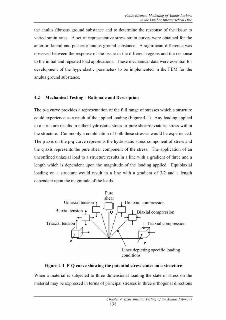
Finite Element Modelling of Anular Lesions in the Lumbar Intervertebral Disc
Chapter 4: Experimental Testing of the Anulus Fibrosus 138
the anulus fibrosus ground substance and to determine the response of the tissue to
varied strain rates. A set of representative stress-strain curves were obtained for the
anterior, lateral and posterior anulus ground substance. A significant difference was
observed between the response of the tissue in the different regions and the response
to the initial and repeated load applications. These mechanical data were essential for
development of the hyperelastic parameters to be implemented in the FEM for the
anulus ground substance.
4.2 Mechanical Testing – Rationale and Description
The p-q curve provides a representation of the full range of stresses which a structure
could experience as a result of the applied loading (Figure 4-1). Any loading applied
to a structure results in either hydrostatic stress or pure shear/deviatoric stress within
the structure. Commonly a combination of both these stresses would be experienced.
The p axis on the p-q curve represents the hydrostatic stress component of stress and
the q axis represents the pure shear component of the stress. The application of an
unconfined uniaxial load to a structure results in a line with a gradient of three and a
length which is dependent upon the magnitude of the loading applied. Equibiaxial
loading on a structure would result in a line with a gradient of 3/2 and a length
dependent upon the magnitude of the loads.
Figure 4-1 P-Q curve showing the potential stress states on a structure
When a material is subjected to three dimensional loading the state of stress on the
material may be expressed in terms of principal stresses in three orthogonal directions
Q
P
Pure shear
Triaxial compression Triaxial tension
Uniaxial tension Uniaxial compression
Biaxial compression Biaxial tension
Lines depicting specific loading conditions

Finite Element Modelling of Anular Lesions in the Lumbar Intervertebral Disc
Chapter 4: Experimental Testing of the Anulus Fibrosus 139
(Section 2.6). When the solid material that is subjected to a general state of stress is
rotated into the orientation of the principal stress state, the shear stresses become zero
and the normal stresses become maximum and minimum values and are referred to as
principal stresses. The deviatoric and hydrostatic stresses on the material are
calculated from the principal and shear stresses. Eqn 4-1 shows the equation for the
general state of stress in a three dimensional material in terms of the hydrostatic and
deviatoric stresses. The deviatoric stress is the difference between the actual stress in
the system and the hydrostatic stress. It is the deviatoric stress that is responsible for
distortion in a loaded structure. The hydrostatic stress is defined in Eqn 4-2.
−−
−+
=
=
σσσσσσσσσσσσ
σσ
σ
σσσσσσσσσ
σHydrzzzyzx
yzHydryyyx
xzxyHydrxx
Hydr
Hydr
Hydr
zzzyzx
yzyyyx
xzxyxx
ij
000000
General Stress Hydrostatic Stress Deviatoric Stress
Eqn 4-1 Equation for general state of stress in a material
3σσσσ zzyyxx
Hydr
++=
Eqn 4-2 Equation for the hydrostatic stress
Using the p-q curve it is apparent that a comprehensive image of the mechanical
behaviour of a material can be obtained by applying various loading conditions. The
Abaqus software will determine hyperelastic parameters for a material based on user
input of test data from biaxial tension/compression, uniaxial tension/compression and
shear loading. It may be seen from Figure 4-1 that these three loading conditions
provide information on a considerable portion of the p-q curve. Since the Abaqus
input requires only these three loading types in order to define a complete hyperelastic
material model, biaxial compression, unconfined uniaxial compression and shear
loading were applied to the anulus fibrosus ground substance in order to quantify its
mechanical response.

Finite Element Modelling of Anular Lesions in the Lumbar Intervertebral Disc
Chapter 4: Experimental Testing of the Anulus Fibrosus 140
Ideally the loading modes used to determine the hyperelastic parameters would be
based on the stress states within the anulus ground substance during physiological
loading. However, extensive data on these stresses was not found in the literature and
since the accuracy of the Mooney-Rivlin hyperelastic material parameters used in the
preliminary FEM was unclear, data for the state of stress in the anulus ground
substance could not be obtained from the FEM. Even so, the biaxial, uniaxial and
shear loading conditions would provide sufficient information to quantify the
hyperelastic parameters.
Testing was carried out on specimens of anulus fibrosus such that the mechanical
behaviour of the anulus ground substance was obtained. In order to achieve this, the
loading applied to the specimens did not apply tension to the collagen fibres in the
anulus. These fibres were tension-only components, so it was acceptable for them to
be loaded in compression. Unconfined uniaxial compression loading was the most
appropriate method to obtain information on the uniaxial loading behaviour of the
anulus fibrosus ground substance.
Pure shear loading was a difficult state of loading to apply to a biological material.
The shear loading which was applied to the anulus ground substance was simple
shear. This was a loading state which involved the translation of two parallel surfaces
of a material in opposite directions. The extension ratio in the maximum principal
direction increased, in the minimum principal direction decreased and in the third
principal direction the extension ratio remained at one. The Abaqus software
specified that the shear loading data was to be pure shear and therefore, the simple
shear stress data was converted to pure shear stress data (Section 5.3).
In the past, biaxial loading on biological tissues has generally been carried out under
tension. In the case of the anulus ground substance the application of tensile loading
would result in load bearing in the collagen fibres. Therefore, biaxial compression
was carried out to quantify the biaxial behaviour of the material.
The anulus fibrosus in the in vivo intervertebral disc experiences both compressive
and tensile stresses during physiological loading. However, it was thought that the
use of compressive rather than tensile loading modes in the experimental testing

Finite Element Modelling of Anular Lesions in the Lumbar Intervertebral Disc
Chapter 4: Experimental Testing of the Anulus Fibrosus 141
would better reflect the stress state within the anulus ground substance. This type of
loading is in the right half of the p-q curve (Figure 4-2).
Figure 4-2 Compressive portion of the p-q curve
4.3 Specimen Harvesting
Sheep discs have been shown to exhibit similar kinematic and biochemical properties
to human discs (Wilke et al., 1997, Reid and Meakin, 2002). Seven intervertebral
discs were sectioned from the frozen lumbar spines of five sheep - two L3/4, one L4/5
and four L6/7 discs were obtained. The posterior elements, spinal cord and
surrounding musculature were removed. A 1-3mm layer of cartilaginous endplate and
vertebral bone on the superior and inferior surfaces of the disc were preserved. While
sectioning the discs from the spines they were kept moist with Ringers solution and
the room temperature was maintained at 20oC. Generally the disc had not thawed by
the time it was isolated from the spine. The discs were then surrounded with Ringers
soaked muslin, sealed in air-tight bags and refrozen to -20oC. Once frozen the
individual discs were set in dental cement in preparation for sectioning into test
specimens (Figure 4-3). The mold for the dental cement was formed from plasticine.
The mold had been frozen at -20oC before placing the disc and uncured dental cement
inside and it was placed in cold water while the uncured dental cement was poured
over the disc. This procedure was carried out to create a heat sink for the exothermic
reaction involved in the curing of the dental cement. The cement was cured for one
hour at room temperature, and then the hardened dental cement with embedded disc
was frozen at -20oC for a further 20 hours.
Compressive region of the p-q curve Q
P

Finite Element Modelling of Anular Lesions in the Lumbar Intervertebral Disc
Chapter 4: Experimental Testing of the Anulus Fibrosus 142
Figure 4-3 Sheep intervertebral disc set in a dental cement plug and mounted on an aluminium bracket to allow for sectioning. The bracket was attached to a
rotating arm to permit cuts of necessary depth and width to be made.
In order to obtain mechanical data for the anulus ground substance in isolation, it was
necessary to ensure that no continuous collagen fibres coupled the two endplates of
the specimens which were tested. In this way, the mechanical response of the
specimen would give information on the response of the ground substance with the
collagen fibres embedded but not actively bearing a load. To ensure there were no
continuous fibres in the specimens, a maximum specimen width was determined using
the average height of the sheep discs and the average angle of inclination of the
collagen fibres in the anulus (Figure 4-4). The required cubic cross-sectional edge
length of the specimens was determined to be 3mm.
Figure 4-4 Determining the specimen width required to ensure there were no continuous fibres connecting the endplates in the specimen
Even though the collagen fibres in the specimens would not actively bear a load they
would still provide some resistance to the applied strain through the frictional
relationship between the fibres and the surrounding soft tissue. This was a desirable
artefact in the stress-strain response of the specimens. If data on the mechanical
α
No continuous fibres
Average Disc
height
α = 30o
Specimen width = 3mm
Endplate and vertebral bone
Anular Saw Blade
The dental cement plug was
attached to a bracket to hold
the disc for sectioning
Sheep intervertebral disc set in dental cement plug

Finite Element Modelling of Anular Lesions in the Lumbar Intervertebral Disc
Chapter 4: Experimental Testing of the Anulus Fibrosus 143
response of the ground substance without any collagen fibres present was obtained,
then it would be necessary to designate a frictional relationship between the ground
substance and the collagen fibres in the FEM. The mechanical data obtained from the
testing of the specimens incorporated this relationship. As highlighted in Section
3.8.2 the reinforcing rebar elements representing the collagen fibres did not allow for
the incorporation of a relationship between these elements and the underlying
continuum elements representing the ground substance. However, since the results of
the mechanical testing included the effects of the interaction between the fibres and
the ground substance, the input of information to define this relationship was not
necessary.
Figure 4-5 A sectioned specimen.
A precision anular microsaw with diamond tipped blade (Figure 4-3) was employed to
section test pieces from the intact disc embedded in dental cement. Cuts were made
parallel to the sagittal and frontal planes through the disc such that the full disc height
and superior and inferior bone layers were preserved in the test specimens (Figure
4-5). The saw mechanism permitted the blade to be advanced after each cut and the
distance advanced could be controlled with an accuracy of 1mm. The blade was
advanced by 3mm after each successive cut in a plane. This produced test specimens
with a cubic cross-sectional width of 3 ± 0.2mm. The disc tissue was kept moist with
Ringer solution during the cutting process.
Once sectioned from the disc the test specimens that contained nucleus material were
discarded. Curing of polymethylmethacrylate was an exothermic reaction which had
been shown to cause tissue necrosis (Lieu, Nguyen and Payant, 2001) and could
Superior cartilaginous endplate
Inferior cartilaginous endplate
Inferior vertebral bone
Radial Direction
Anulus Fibrosus
Superior vertebral bone

Finite Element Modelling of Anular Lesions in the Lumbar Intervertebral Disc
Chapter 4: Experimental Testing of the Anulus Fibrosus 144
involve temperature increases as high as 35oC. To ensure damaged specimens weren't
used for testing, anulus specimens from the peripheral disc were discarded as these
were in direct contact with the dental cement during curing. Anulus specimens were
labelled according to disc region (anterior, lateral or posterior), wrapped in Ringers
soaked muslin, sealed in clip seal bags and frozen to -20oC. Specimens were frozen
for a maximum of five days before being tested.
The number of specimens obtained from the disc regions varied:
• four - six specimens obtained from the anterior disc;
• four - six specimens obtained from the lateral disc; and
• three - five specimens obtained from the posterior disc.
Uniaxial compression, biaxial compression and simple shear tests were carried out on
specimens from each region of the disc. All specimen dimensions were measured
before testing. Stress and strain was calculated based on the unstressed dimensions.
4.4 Biaxial Compression Testing Methods and Equipment
The following sections provide details of the equipment and procedures employed for
the biaxial compression experimental testing. A testing rig was designed, built and
commissioned to carry out biaxial compression loading on the sheep anulus
specimens. This section provides a description of the design rationale and details, on
the proof testing of the biaxial compression equipment and the methods employed to
obtain biaxial compression data for the anulus fibrosus specimens.
4.4.1 Principle of operation
A novel testing rig was designed and built to carry out biaxial compression. The
design objective for the rig was to apply a hydrostatic pressure to the specimen and
then unload it along one axis to obtain a state of biaxial compression.

Finite Element Modelling of Anular Lesions in the Lumbar Intervertebral Disc
Chapter 4: Experimental Testing of the Anulus Fibrosus 145
A B
Figure 4-6 The assembled biaxial testing rig A. With lid in place; B. With lid removed.
The developed rig was a stainless steel rectangular vessel, which could be filled with
Ringers' solution and pressurised (Figure 4-6). Two viewing windows were inserted
in two opposite walls of the vessel. The remaining walls provided attachment sites
for durable nylon thread, the ends of which were glued to the bone surfaces on the
specimen. Thus the specimen was suspended in the centre of the vessel and could be
viewed through the windows. It was necessary for the vessel sides to be planar so the
viewing windows could be inserted and to ensure the specimen was aligned parallel to
the direction of viewing.
One of the nylon threads connected the specimen directly to a wall. The other piece
of nylon connected the specimen to the end of a glass ceramic piston running in a well
polished bore in the opposite wall of the box. The cross-sectional area of the piston
was equal to the bone surface area of the specimen. The clearance between the bore
and piston was sufficient to allow the fluid in the box to leak when the fluid pressure
increased above gauge pressure. A low piston weight allowed it to be readily
suspended on a layer of fluid when the pressure in the box was increased. The polish
on the bore and piston surfaces and the use of Ringers' solution as lubricant meant
there was limited frictional resistance between bore and piston. A pressure inlet in the
lid of the box was connected to an air compressor through a high precision pressure
regulator which ensured accurate control of the pressure in the box.
When the pressure to the box was increased, this pressurised a 10mm air gap in the
Viewing windowsAttachment sites for nylon thread

Finite Element Modelling of Anular Lesions in the Lumbar Intervertebral Disc
Chapter 4: Experimental Testing of the Anulus Fibrosus 146
top of the sealed box and in turn pressurised the solution. The pressure on the six
faces of the specimen and on the end of the piston was equivalent to the water
pressure. Because the area of the specimen bone face and the piston end were equal
and they were connected by an inextensible nylon thread, the forces on each face
would be equal in magnitude and opposite in direction. Thus, there would be no
compressive force acting on the specimen in the axis of the piston. However, the
compressive force in the other two axes would not be affected.
4.4.2 Design details and pressure vessel components
The walls of the pressure vessel were manufactured from 10mm stainless steel and the
viewing windows were 19mm thick standard glass. PVC brackets were used to hold
the glass viewing windows in position.
Refer to Appendix B for detailed engineering drawings and three dimensional solid
models of the pressure vessel components.
4.4.2.1 Maximum vessel pressure and design pressure
The relevant Australian Standard for non-serially produced pressure vessels was
AS1210-1997. This standard required that a maximum vessel pressure and design
pressure be determined. The maximum vessel pressure was the pressure which could
reasonably be expected to be reached during operation of the vessel and the design
pressure was to be greater than the maximum pressure and smaller than the pressure
setting on any pressure relief valves in the vessel.
Because biaxial compression loading had not previously been carried out on
specimens of anulus fibrosus ground substance it was difficult to determine a
maximum vessel pressure for the testing rig. Therefore, three pilot experiments were
carried out under uniaxial compression loading in order to determine the order of
magnitude of the pressures which would be applied to the material. From these tests
it was found that the maximum uniaxial compressive stress applied to the tissue was
approximately 0.28MPa. It was considered that the tissue would be stiffer under

Finite Element Modelling of Anular Lesions in the Lumbar Intervertebral Disc
Chapter 4: Experimental Testing of the Anulus Fibrosus 147
biaxial compression and therefore, a scaling factor of 2.5 was applied to this
maximum pressure in order to determine an approximate maximum vessel pressure.
The maximum pressure was 0.7MPa.
A design pressure of 120psi or 0.827MPa was employed for all design calculations on
the box. This pressure was the supply pressure from the laboratory compressor.
4.4.2.2 Vessel walls
Originally the vessel walls were to be manufactured from perspex to allow the
deformation of the specimen to be viewed. However, this material selection was later
altered to 316 stainless steel. It was considered that the stainless steel demonstrated
more favourable mechanical properties than the perspex and additionally it could not
be assured that the specimen deformation viewed through the Perspex would not be
distorted. The steel wall thickness was 10mm.
The dimensions of the pressure vessel ensured the fluid pressure above the specimen
did not cause a high prestress and that there was sufficient fluid above the specimen
for the duration of the loading. The head of fluid above the specimen was
0.444x10⁻³MPa. This prestress on the specimen was considered to be negligible.
To seal the lid of the pressure vessel, a rubber gasket was cut to size.
The pressure vessel was designed in accordance with AS1210-1997. The relevant
requirements of this standard were the design material strength, the minimum wall
thicknesses and that the pressure vessel contained a pressure relief device.
• Design tensile strengths for materials were to be ¼ the specific tensile strength
of the material. The design tensile strength of the steel was 104MPa.
• The minimum wall thickness was calculated for a pressure vessel with non-
circular ends. This was 6.66mm. The 10mm thick stainless was considered to
be acceptable.

Finite Element Modelling of Anular Lesions in the Lumbar Intervertebral Disc
Chapter 4: Experimental Testing of the Anulus Fibrosus 148
• A minimum wall thickness was calculated for the walls with viewing windows
inserted. This was 9.07mm. The 10mm thick stainless steel walls were
acceptable.
• A pressure relief valve was incorporated into the pressure line connecting the
vessel to the compressor.
It was not possible to carry out a stress analysis of the pressure vessel using standard
theories of thin-walled pressure vessels. The vessel was not thin-walled; it was not a
continuous vessel, rather was an assembly of parts; and it was neither circular nor
elliptical. Stress analysis of the pressure vessel was carried out using Roark’s (1989)
formulae for stresses in plates with varied geometries and boundary conditions.
Equations for the stress in a flat rectangular plate, with fixed edges and a uniform
surface pressure were employed to determine the maximum bending stress in the
vessel walls. The bending stress in the walls with the viewing windows was increased
by a stress concentration factor to account for the holes in the faces.
The maximum stress in the long walls, the lid and the base was 45MPa and in the
viewing window walls, the maximum stress was 96MPa. These values were
compared with the design tensile strength, 104MPa, and the yield strength, 170MPa,
of the steel. It was apparent that the bending stress in the walls was acceptable.
4.4.2.3 Fasteners
Fasteners for the pressure vessel were M6 x 1.0 steel socket cap screws. High tensile
strength socket cap screws were used to fasten the lid of the vessel to the walls but
stainless steel screws were used in all other locations on the vessel.
The design calculations for the fasteners in the pressure vessel included calculation of
the minimum engagement depth of the screws in the vessel walls to avoid thread
stripping, calculation of shear stresses across the shaft of the screw due to the wall
junctions and determination of the necessary number of fasteners on each wall. The
threaded length of the cap screws was 25mm and the engagement length in the vessel

Finite Element Modelling of Anular Lesions in the Lumbar Intervertebral Disc
Chapter 4: Experimental Testing of the Anulus Fibrosus 149
walls was approximately 15mm which was significantly higher than the calculated
minimum length.
The number of fasteners on the edges of each side of the vessel was determined on the
basis of calculations of the stress states in the bolts with a safety factor of 1.5. A
comparison of these stresses with the yield strength and shear strength of stainless
steel and high tensile strength steel ensured that the working stress in the cap screws
was within the strength range of the materials.
4.4.2.4 Viewing windows
The viewing windows were standard glass plugs with a thickness of 19mm. They
were fastened into two opposite walls of the vessel and sealed with an O-ring.
To ensure there were no discontinuities or disruptions in the glass plugs that could
result in inaccuracies in the image viewed through the windows, the plugs were
rotated while viewing a straight line drawn on the wall. If there were discontinuities
in the glass, a distorted view of the straight line would have been found. There was
no distortion of the line in any orientation of either of the glass plugs. Calculations
were carried out to determine whether there would be any distortion in the image
viewed through the viewing windows once the specimen was in the assembled vessel.
These calculations were based on Snell’s Law for reflected/refracted light. It was
found that no distortion of the image would occur if the surfaces of the glass viewing
windows were parallel in the assembled vessel and if the windows were also parallel
to the projection screen for the image. A precision steel metrology rod with a
diameter of 10.00mm was measured whilst positioned in the assembled vessel. The
diameter of this rod was measured on a Sigmoscope (Section 4.4.5.2) with three sets
of ten measurements. The average error in the measured diameter was 0.005mm.
This was a good agreement between the measured diameter and the correct diameter.
The shear and bending stresses on the glass in the pressurised vessel were calculated
and compared with the tensile and shear strength of glass ceramics. There was no risk
of failure of the glass windows.

Finite Element Modelling of Anular Lesions in the Lumbar Intervertebral Disc
Chapter 4: Experimental Testing of the Anulus Fibrosus 150
4.4.2.5 Attachment of specimen to nylon cord
The specimens were attached to the nylon cord using cylindrical dental cement plugs
(Figure 4-7) with an outer diameter of 3mm. One end of a piece of nylon cord was set
in the cement and the other end was fastened either in the titanium cap of the ceramic
piston or on the locator at the end of the adjustment knob (Figure 4-11).
Figure 4-7 Dental cement plug for attaching specimen to nylon cord
4.4.2.6 Leaking piston and bore insert
The piston diameter was selected such that the cross-sectional area of the piston was
equivalent to the cross-sectional area of the bone faces on the specimens. The
equivalence of these surface areas ensured that the force acting on each face was
equal in magnitude but opposite in direction and thereby unloaded the specimen along
the longitudinal axis acting through the two bone faces of the specimen. This
unloaded state of the specimen in the axial direction is demonstrated using a free-
body-diagram of the specimen in the assembled pressure vessel (Figure 4-8). The
tension in the right nylon cord at the fixed end was the same as the tension in the
opposite end of the cord at the face of the specimen. This tension was created by the
pressure acting on the face of the specimen. Also, the tension in the left nylon cord
which acted on the face of the piston was of the same magnitude (but opposite
direction) as the tension acting at the specimen face to which it was attached. Thus,
the specimen experienced no tensile or compressive stress in the axial direction. The
bone faces of the specimens were cubes with edge lengths of 3mm. Therefore, in
order for the cross-sectional area of these faces to be equal the piston diameter needed
to be 3.385mm. This component was manufactured with a diameter of 3.40mm.

Finite Element Modelling of Anular Lesions in the Lumbar Intervertebral Disc
Chapter 4: Experimental Testing of the Anulus Fibrosus 151
Figure 4-8 Schematic of piston attachment in pressure vessel (not to scale). ‘P’ represents the pressure on the face of the specimen and piston due to the
pressurised fluid. ‘T’ represents tension in the nylon cord and is an equal but opposite force at the ends of the specimen, at the wall of the vessel and at the face
of the piston.
The piston design and the piston-bore clearance were selected to ensure that there was
sufficient pressurised fluid to surround the piston but that the flow rate did not deplete
the fluid volume in the vessel too quickly. Potential piston designs had incorporated
circumferential and longitudinal grooves that were intended to encourage fluid to
surround the piston and separate it from the walls of the bore. However, it was
suspected that the longitudinal grooves may create asymmetrical loading of the piston
once it was under fluid pressure. The pistons with circumferential grooves were not a
practical design. The groove corners created significant stress concentrations which
made manufacture on the lathe difficult and increased the potential for piston
breakage during setup of the testing rig. Therefore, the final piston design was a
straight sided shaft (Figure 4-9).
As the biaxial pressure on the specimen increased, the radial and circumferential
dimensions of the specimen decreased and the axial dimension increased. Therefore,
it was necessary for the piston to move in the bore so that the nylon cord connecting
the piston and specimen remained tensioned. It was imperative that the movement of
the piston through the bore be as near to frictionless as possible. This was achieved
by including a small clearance in the bore such that fluid leaked from the pressure
vessel during loading. The piston was manufactured from Macor Machinable® Glass
Ceramic. This was a material which possessed good machinability for high precision
components, had zero porosity, was non-corrosive and was capable of being
Leaking Piston
Vessel Walls
T
T T
T
P P Leaking Fluid through bore clearance
Axial direction of specimen
P
P
P

Finite Element Modelling of Anular Lesions in the Lumbar Intervertebral Disc
Chapter 4: Experimental Testing of the Anulus Fibrosus 152
machined to high tolerances. Therefore, it was possible to obtain a low roughness
surface finish – Ra = 0.7µm – to encourage a low friction relationship between the
piston and the leaking fluid.
Using the theory of laminar fluid flow between two parallel plates (Eqn 4-3), the
bore-piston clearance was determined.
Lp
lQ a
..12.3
µ∆
=
Where, a = distance between the plates
p∆ = pressure variation along the length of the plate
L = depth of the plate
l = width over which the plates are facing
µ = viscosity
Q = volume flow rate
Eqn 4-3 Laminar fluid flow between parallel plates
In the case of the piston and bore,
a = clearance between the piston and bore
p∆ = pressure variation along between the average pressure in the
box and atmospheric pressure. This average pressure was half
the design pressure.
= average pressure, 0.4135 – atmospheric, 0.101MPa
= 0.3125x10⁶ N/m2
l = the circumference of the piston, πD
= 10.68x10⁻³ m
L = length of the bore – even though the piston was capable of
moving through the bore, these calculations were based on the
assumption that the piston was completely inside the bore
= 0.025 m
µ = viscosity of Ringers solution which was approximated as the
viscosity of water
= 8x10⁻⁴ kg/ms

Finite Element Modelling of Anular Lesions in the Lumbar Intervertebral Disc
Chapter 4: Experimental Testing of the Anulus Fibrosus 153
Q = the volume flow rate was selected to ensure that there would
be sufficient fluid in the vessel for a biaxial test to be carried
out for 30 minutes. The height of saline solution above the
specimen initially was 35mm.
= (0.035x0.110x0.150) m3 / 45 minutes
= 2.139x10⁻⁷ m3/s
Using these variables, the calculated clearance, a , was 0.022mm. Therefore, the
necessary bore diameter was 3.44mm. Such a small diameter reamed over a length of
25mm required notable manufacturing expertise to ensure concentricity of the bore
over its length. This was achieved by the QUT mechanical workshop. The bore was
reamed to ensure a high quality surface finish.
The assumption of laminar flow required that the fluid flow possessed a Reynolds
number < 1400 and that it was fully developed. It was reasonable to expect that with
a sufficiently small clearance, the fluid velocity would be low and the Reynolds
number below 1400. To make certain the flow was fully developed, it was ensured
that the clearance was very much smaller than the length of the cylinder.
In order to attach the nylon cord, a titanium cap was manufactured and fastened to the
end of the ceramic piston (Figure 4-9). The material choice for the cap was based on
the low corrosive properties of the titanium and its high strength-to-weight ratio. The
surface finish obtained on the cap was 0.2µm and it was attached to the ceramic piston
using LOCTITE® 324 acrylic adhesive and 7075 activator.
Figure 4-9 Ceramic piston with titanium cap glued to the end.
The bore insert was manufactured from stainless steel and inserted into one wall of
the pressure vessel (Figure 4-10).
Titanium Cap
Ceramic piston
The specimen was glued to the flat face of this dental cement plug

Finite Element Modelling of Anular Lesions in the Lumbar Intervertebral Disc
Chapter 4: Experimental Testing of the Anulus Fibrosus 154
A B
C
Figure 4-10 Assembly of pressure vessel wall, bore insert and glass ceramic piston A. Solid model assembly; B. Sectioned view of assembly, sectioned along a vertical axis through the centre of the piston; C. Ceramic piston and bore insert
in the assembled pressure vessel – viewing inside vessel
4.4.2.7 Adjustment knob for accurate orientation of the specimens
In order to control the orientation of the specimen while it was suspended in the
Ringers solution, an adjustable fixture was placed on the inside of the wall to which
the nylon cord was fixed (Figure 4-11). This fixture was rotated using an adjustment
knob on the outer wall of the vessel. This permitted deformation measurements to be
taken in both the radial and circumferential directions of the anulus specimens and
ensured the specimen could be orientated such that either the radial or circumferential
direction was perpendicular to the viewing windows.
Pressure vessel wall
Bore insert
Piston

Finite Element Modelling of Anular Lesions in the Lumbar Intervertebral Disc
Chapter 4: Experimental Testing of the Anulus Fibrosus 155
A B
C
Figure 4-11 Adjustment knob assembly A. Adjustment knob viewed from outside the vessel; B, C. Adjustable fixture viewed from inside the vessel
4.4.3 Proof testing
The Australian standard AS1210-1997 stated that the suitability and safety of pressure
vessels which were not adequately dealt with in the standard could be established by
either:
• Demonstrating successful performance of a prototype pressure vessel
subjected to similar conditions;
• Carrying out rigorous mathematical stress analysis, including FE analysis;
and/or
• Carrying out a proof test of the vessel. (Pressurise the vessel to a test pressure
of twice the design pressure for 15 seconds and examine the vessel for leakage
or signs of deformation.)
An extensive stress analysis was carried out during the design of the vessel
components. The proof test was carried out once the pressure vessel components
Attachment site for nylon cord
Teflon washer for low friction during rotation
Adjustment knob

Finite Element Modelling of Anular Lesions in the Lumbar Intervertebral Disc
Chapter 4: Experimental Testing of the Anulus Fibrosus 156
were manufactured and assembled. AS1210 stated that single walled vessels should
be loaded to a pressure Ph during the test.
ffP h
hP ×= 5.1
where, P = design pressure = 150psi = 1.03MPa
hf = design strength at test temperature
f = design strength at design temperature
Therefore, Ph = 225psi = 1.55MPa
Eqn 4-4
The pressure vessel was subjected to a maximum pressure of 300psi (2.07MPa) and
held constant at this pressure for 30 seconds. At 150 psi and 225 psi, the condition of
the vessel was assessed – there was no visible leakage from the vessel and all
components of the vessel were undeformed and intact. At 300 psi there was a small
leakage from the screws on the lid, but this was eliminated by further tightening. All
components of the vessel were undeformed and intact.
It was concluded that the proof testing of the pressure vessel was successful and it
was acceptable for use in the biaxial compression testing of the anulus fibrosus
specimens. The hazard rating of the pressure vessel was obtained from AS4343-1999
and was a hazard level E which was classified as ‘negligible’.
4.4.4 Setup of equipment
Until the time of testing, the specimens were frozen in Ringers soaked muslin and
sealed in plastic bags. Assembly of the pressure vessel required 30 minutes during
which time the anulus specimen was wrapped in Ringers soaked muslin or immersed
in Ringers solution in the vessel. By the time the biaxial compression tests were
carried out the specimen was completely thawed. The assembled pressure vessel was
located on the table of the Sigmoscope profile projector (Herbert Controls and
Instruments Ltd, Letchworth, England) (Figure 4-12) ensuring the viewing windows
were parallel to the projector screen and the specimen was orientated in the vessel so

Finite Element Modelling of Anular Lesions in the Lumbar Intervertebral Disc
Chapter 4: Experimental Testing of the Anulus Fibrosus 157
that the deformation would be measured in the desired axis of the anulus – that is,
radial or circumferential deformation.
Figure 4-12 Assembled pressure vessel
4.4.5 Measurement of biaxial compressive stress and strain
Details of the equipment used to measure the biaxial compressive stress and the
resulting deformation of the anulus fibrosus specimens are provided in the following
sections.
4.4.5.1 Choice of pressure regulator
The compressive stress applied to the specimen was equivalent to the pressure of the
Ringers solution surrounding it. This pressure was determined using a digital Druck
pressure calibrator (Model: DPI 705, GE Druck Ltd, Leicester, UK) and the vessel
was pressurised using a precision pressure regulator. It was important to use a
pressure regulator with a maximum pressure similar to the maximum operating
pressure during the testing. If the maximum pressure on the regulator was too high
then its accuracy was reduced and low pressures of 0 to 10psi would not be
adequately controlled. Additionally, because the pressure vessel was designed to leak
during operation, the regulator needed to maintain a constant pressure in the box
despite the loss of fluid.

Finite Element Modelling of Anular Lesions in the Lumbar Intervertebral Disc
Chapter 4: Experimental Testing of the Anulus Fibrosus 158
A Norgren zinc alloy precision regulator (Model:11-818, IMI Norgren Ltd,
Staffordshire, UK) with a maximum pressure of 60 psi and an accuracy of 0.435 psi
was employed. This regulator provided excellent control over the pressure in the
vessel for the full range of pressures applied during testing. (The pressure regulator
was manufactured using imperial measuring units, therefore, pressure units of psi are
used in Sections 4.4.6.1 and 4.4.6.2 to convey details of pressures measured using this
device. 1psi = 0.0689MPa)
4.4.5.2 Profile projector
To measure the deformation of the specimen under load, a Sigmoscope profile
projector was used. This equipment was capable of providing high precision
measurements of specimen dimensions by shining a light source across the item to be
measured and projecting the shadow of the item onto a viewing screen. By moving
the stage on which the item was positioned it was possible to obtain a digital readout
for the necessary linear dimension.
In the case of the biaxial compression testing, the light source was projected through
the viewing windows of the vessel (Figure 4-13 A) and a projected image of the
deformed specimen was obtained (Figure 4-13 B). The specimen was orientated
using the positioning knob, such that either the radial or circumferential direction in
the anulus was perpendicular to the viewing windows, enabling these dimensions to
be measured (Figure 4-13 B). There was no distortion of the image as a result of the
light beam passing through the Ringers solution so long as the solution was
homogeneous.

Finite Element Modelling of Anular Lesions in the Lumbar Intervertebral Disc
Chapter 4: Experimental Testing of the Anulus Fibrosus 159
A B
Figure 4-13 Measurement of specimen deformation during biaxial compression; A. Specimen through viewing window; B. Image projected onto the Sigmoscope
screen. Moving the machine table allowed the linear dimensions to be determined
4.4.5.3 Data acquisition - hydrostatic pressure and deformation
Data on the anulus fibrosus ground substance response to both initial loading and
repeated loading on a single specimen was obtained. A single specimen was tested
seven times. The specimen was permitted to recover for 15 minutes between each
test. Data for the initial specimen width in either the radial or circumferential
direction was recorded. It was expected that the deformation in these directions
would differ but it was not practical to measure the deformation in both directions on
a single specimen. Orientating the specimen in both directions at a single pressure
resulted in the specimen remaining at the pressure for too long. Creep in the tissue
caused its deformation to continue to vary at this constant pressure and it was not
possible to obtain reliable and repeatable results. Of the 24 specimens tested with
biaxial compression, 14 were orientated so the deformation was measured
circumferentially.
4.4.6 Commissioning of pressure vessel
Commissioning of the pressure vessel involved ensuring the pressure applied to the
inner face of the piston was accurate and ensuring the testing technique was
repeatable.
Deformed width measured
Loose tissue from specimen – not measured

Finite Element Modelling of Anular Lesions in the Lumbar Intervertebral Disc
Chapter 4: Experimental Testing of the Anulus Fibrosus 160
4.4.6.1 Force applied to the piston
In order to ensure that the force acting on the inner face of the piston was accurate, the
vessel was assembled with the outer face of the piston in contact with a 500N
Hounsfield load cell (Hounsfield Test Equipment, Red Hill, England). Water in the
vessel was incrementally pressurised and the force output from the load cell recorded.
Five sets of pressure measurements were obtained and the pressure was increased by
10 psi between 0 and 96.85 psi in each set. The pressure was measured with the
digital Druck pressure calibrator.
The results were graphed as force vs. applied pressure. A line of best fit was
determined. An average error of 2.10% existed between the measured force and the
force which was calculated on the basis of the pressure applied and the cross-sectional
area of the piston. The inaccuracy between these results was firstly a result of the
shear stress on the walls of the piston and bore and secondly, due to the calibration of
the Hounsfield load cell.
The wall shear stresses were determined over the range of pressures using Eqn 4-5.
yu∂∂
= µτ and
( )cylp
yu
−
∆=
∂∂ 2..
21µ
where, u = velocity of the fluid
p∆ = pressure variation along length of piston
l = length of piston
µ = viscosity of the fluid
c = clearance between the piston and bore
y = distance measured across the clearance c
Eqn 4-5 Shear stress and the velocity profile for flow between infinite parallel plates
The shear force at each pressure was subtracted from the measured force. This
improved the average error between the measured force and the calculated force to a
value of 0.93%. The error between the calculated force and the improved measured

Finite Element Modelling of Anular Lesions in the Lumbar Intervertebral Disc
Chapter 4: Experimental Testing of the Anulus Fibrosus 161
force increased with increasing pressure and was a maximum of 0.081N at 96.85 psi.
This average error between the forces was improved further by determining the
calibrated force from the Hounsfield load cell.
A series of weights between 1 and 500g were placed on the Hounsfield 500N load cell
and the force readout recorded. The variation between the calculated forces
(calculated using gravity) and the measured forces were determined. Over this load
range the relationship in Eqn 4-6 was found.
HounsfieldCorrect ForceForce ×= 988.0
Eqn 4-6 Relationship between the force output from the 500N Hounsfield load cell and the correct force
This result indicated that the Hounsfield load cell slightly overestimated the force
applied to the piston by the pressurised fluid (Figure 4-14). Using this relationship
the error between the measured forces and the calculated forces was improved to an
average of 0.37%.
01234567
0 20 40 60 80 100 120Pressure (psi)
Forc
e (N
)
Measured Force - Shear Force Hounsfield corrected calculated force
Figure 4-14 Comparison of the improved measured force and the calculated force which was manipulated to account for the calibration of the Hounsfield
500N load cell.
It was concluded from these measurements that the piston would apply an acceptably
accurate load to the specimen during the biaxial compression loading.

Finite Element Modelling of Anular Lesions in the Lumbar Intervertebral Disc
Chapter 4: Experimental Testing of the Anulus Fibrosus 162
4.4.6.2 Biaxial compression of EVA foam
A cubic piece of closed cell EVA foam was tested to determine the repeatability of
the testing technique. During nine separate biaxial experiments the test piece was
loaded to a maximum pressure of 30 psi in approximate pressure increments of 5 psi.
A recovery time for EVA foam was not known therefore, the specimen was permitted
to relax for 1.75-2.0 hours between tests.
The pressure was increased incrementally because the measurement of the test piece
deformation was not automated. The testing procedure for biaxial compression
involved obtaining a pressure with the regulator, the specimen deformation being
measured on the Sigmoscope, the deformation recorded and the pressure then
manually increased further.
The deformation recorded for the biaxial compression testing was the minimum width
of the test piece at each pressure. (Figure 4-15)
Figure 4-15 Measuring the deformation during biaxial compression testing
This deformation was normalised with the width measured at the gauge pressure, do to
obtain the extension ratio. This value was referred to as the extension ratio even
though the deformation of the specimen involved compression. The use of the term
extension ratio was in keeping with the terminology used in Chapter 5 to define the
constitutive equations for the hyperelastic strain energy equation.
Increasing pressure
Length increase
do
dP1
dP2
P1 applied
P2 applied
Gauge
Dental cement plug with nylon cord attached
EVA foam

Finite Element Modelling of Anular Lesions in the Lumbar Intervertebral Disc
Chapter 4: Experimental Testing of the Anulus Fibrosus 163
The change in specimen width was used to determine the biaxial strain in the
specimen. The deformed edges of the test piece were not regular and the minimum
width measured was generally not at the midpoint along the specimen. However, the
observed minimum points on each edge tended to remain in the same location
between tests, demonstrating some repeatability of the testing technique. Extension
of the test piece in the direction of the nylon cord was observed as a result of the
compression in the other two axes; however, this deformation was not measured.
2.52.7
2.93.13.3
3.53.7
0 10 20 30Pressure (psi)
Min
imum
Wid
th (m
m)
1st Test 2nd Test 3rd Test4th Test 5th Test 6th Test7th Test 8th Test 9th Test
Figure 4-16 Pressure vs. minimum width for biaxial compression testing on EVA foam
Nine sets of measurements were made for the EVA foam. These tests showed a
reduction in stiffness for the first and second load cycles. It was considered that the
variation in the response of the foam in the first and second tests was a result of the
consolidation of the material. When subjected to repeated loading, foams are known
to precondition which involves a reduction in the stiffness of the material until a
repeatable response is obtained (Nusholtz et al., 1996). The data for the EVA foam
showed a repeatable trend for the final seven tests (Figure 4-16). This implied that the
response of the EVA foam specimens was similar to the reported response for foams
and indicated that the biaxial compression testing method and measurement
techniques could provide repeatable results. On the basis of the tests on EVA foam, it
was apparent that the biaxial compression measurement techniques could produce a
repeatable response and therefore, they were employed to test specimens of anulus
fibrosus.

Finite Element Modelling of Anular Lesions in the Lumbar Intervertebral Disc
Chapter 4: Experimental Testing of the Anulus Fibrosus 164
4.5 Uniaxial Compression and Simple Shear
Fixtures were designed to attach to existing materials testing equipment in order to
carry out uniaxial compression and simple shear tests. Details of the testing methods
and equipment used for the uniaxial compression and simple shear tests are provided
in the following sections.
4.5.1 Testing equipment
The following sections detail the test equipment used to carry out the uniaxial
compression and simple shear experiments.
4.5.1.1 Uniaxial compression
Uniaxial compression of the anulus fibrosus specimens was carried out on a
Hounsfield testing machine using a 500N load cell. The full scale deflection of the
load cell was set to 5%, therefore, the maximum load applied was 25N. Accuracy of
this load cell for small load values was outlined in section 4.4.6 and the relationship
between the force output from the load cell and the correct force was defined in Eqn
4-6. This relationship was taken into account in the analysis of the uniaxial
compression results.
The bone faces on the superior and inferior surfaces of the specimen were glued to the
fixtures on the load cell and on the crosshead of the machine with Loctite® 401. This
specimen orientation created compressive loading in the axial direction. To determine
the mechanical response of the tissue to both initial and repeated loading, five tests
were carried out on each specimen and the specimen was permitted to relax for 5
minutes between each test. The specimen was kept hydrated between tests and during
testing using a squirt bottle of Ringers solution and by wrapping it in Ringers soaked
muslin and a plastic sheet.

Finite Element Modelling of Anular Lesions in the Lumbar Intervertebral Disc
Chapter 4: Experimental Testing of the Anulus Fibrosus 165
4.5.1.2 Simple shear
Simple shear loading was carried out using the Hounsfield testing machine equipped
with a 5N load cell. Accuracy of this load cell was tested using a spring of known
spring constant. The spring constant measured using the 5N load cell was 0.623%
higher than the correct value. This was considered to be an acceptable level of
accuracy.
Figure 4-17 Hounsfield attachments to apply simple shear
The load cell could measure only tensile loads, therefore, fixtures were designed and
manufactured to apply simple shear (Figure 4-17).
The fixtures were manufactured from aluminium alloy to minimise weight. The
upper fixture was suspended from the load cell therefore, it was necessary that its
weight be sufficiently low to be tared by the load cell. Anulus specimens were
attached to the opposing faces of the fixtures using Loctite® 401. When the
crosshead was driven downward a state of simple shear was created in the specimen.
Attachment to 5N load cell
Upper shear fixture
Lower shear fixture
Specimen

Finite Element Modelling of Anular Lesions in the Lumbar Intervertebral Disc
Chapter 4: Experimental Testing of the Anulus Fibrosus 166
The shear force could have been applied to the specimens in either a circumferential
direction or a radial direction (Figure 4-18). Fujita et al. (2000) carried out shear
testing in all three anulus directions and found that the shear modulus in the radial and
circumferential directions were similar and in the axial direction it was twice the
modulus in the other two orientations. It was postulated in the current study, that this
significant variation in shear modulus with specimen orientation was a result of the
loading of continuous collagen fibres. Such significant variations in stiffness would
not be expected if the ground substance was tested.
Figure 4-18 Anulus fibrosus showing potential directions of shear
If the simple shear force on the specimens was aligned with the radial direction
(Figure 4-18), this may have resulted in separation of the lamellae. Thus the simple
shear response obtained would be partially dependent on the bonding strength of the
adjacent lamellae. Simple shear loading in either the axial direction or the
circumferential direction would not have caused separation of the lamellae; however,
it was not possible to load the specimens in the axial direction because of the layer of
vertebral bone that was preserved on the superior-most and inferior-most faces of the
specimens. It was considered that application of the simple shear load to the
specimens in a circumferential direction would be most appropriate.
In order to determine the response of the tissue to initial and repeated loading, the
specimens were loaded five times, with a five minute recovery period between each
test. The specimens were kept hydrated during the tests and the recovery time using
Ringers solution, Ringers soaked muslin and plastic wrap.
Axial directionCircumferential direction
Radial direction

Finite Element Modelling of Anular Lesions in the Lumbar Intervertebral Disc
Chapter 4: Experimental Testing of the Anulus Fibrosus 167
4.5.2 Maximum strains applied during testing
In order to obtain a close fit between the hyperelastic model representing the anulus
ground substance and the experimental response of the material under load, it was
necessary to perform experiments over the same range of strains as would be expected
to occur physiologically. Pilot FEM analyses showed that hyperelastic parameters fit
to stress-strain data below the maximum strain observed in the disc, exhibited a good
fit for the experimental response only to strains for which the hyperelastic parameters
had been fit. At higher strains, the hyperelastic model did not display good agreement
with the experimental data.
The maximum strains observed in the preliminary FEM were for the full flexion
loading. Engineering strains as high as 4.2 were found. The maximum strain applied
during the compressive experimental testing could not reasonably exceed 60-70%
without introducing some tension in the collagen fibres of the anulus. Simple shear
loading was carried out to maximum strains of 50-80% and the maximum biaxial
compressive strain was 30%.
4.6 Strain Rate during Uniaxial Compression and Simple Shear Loading
The material testing carried out on anulus specimens aimed to simulate physiological
strain rates. These rates would result in no fluid loss or volume change in the
material. This was in keeping with the assumption of incompressibility employed for
the hyperelastic material description in the anulus fibrosus ground substance. No
evidence was found for the value for physiological loading rates. Several
experimental studies had been carried out on specimens of anulus fibrosus which
employed strain rates ranging from 0.00009 sec-1 and 0.005 sec-1 (Fujita et al., 1997;
Ebara et al., 1996; Acaroglu et al., 1995; Best et al., 1994; Skaggs et al., 1994; Wu
and Yao, 1976). The lower strain rates were intended to ensure the fluid drag through
the matrix of the anulus fibrosus was limited. Therefore, to ensure no fluid movement
within the specimens tested in the current study, a strain rate well above the range
0.00009 sec-1 to 0.00012 sec-1 was employed. Studies which employed strain rates
between 0.00012 sec-1 and 0.005 sec-1 were not intending to simulate the
Finite Element Modelling of Anular Lesions in the Lumbar Intervertebral Disc
Chapter 4: Experimental Testing of the Anulus Fibrosus 168
physiological condition and made no mention of quantifying the mechanical response
of the material for the in vivo condition.
In order to determine a suitable strain rate to employ in the mechanical testing,
experiments were carried out under uniaxial compression and simple shear at 0.10
sec-1, 0.01 sec-1 and 0.001 sec-1.
4.6.1 Procedure for testing to determine the tissue response to varied strain
rates
Three specimens of anulus fibrosus were specifically tested to investigate the effects
of various strain rates. Individual specimens were tested under uniaxial compression
and simple shear. It was not possible to test the specimens using biaxial compression
as they could not be loaded at a higher strain rate than 0.01 sec-1. A similar procedure
to that used for the stress-strain experiments was employed (section 4.5.1). The
maximum strain in the strain rate tests was approximately 20% as this was the lower
threshold of the derangement strain. For the purpose of this study, the derangement
strain has been defined as any damage to the anulus fibrosus ground substance that
causes a reduction in the observed stiffness of the material, but which does not
prevent the tissue from bearing a load during subsequent loading. Further results for
these strains are provided in Section 4.8.
The specimens were tested four times at each strain rate. The first and second tests –
test a and b – were carried out 5 minutes apart in keeping with the procedure
employed for the stress-strain experiments. The specimen was then permitted to
recover for one hour in order to remove any viscoelastic effects in the tissue and to
permit absorption of any pore fluid lost during the first tests. After recovery, the
specimen was retested two times, 5 minutes apart – test c and d. Results for three
strain rates were compared – 0.001 sec-1, 0.01 sec-1 and 0.10 sec-1. The specimens
tested at 0.001 sec-1 were retested an additional two times, 5 minutes apart, after a one
hour recovery – test e and f.

Finite Element Modelling of Anular Lesions in the Lumbar Intervertebral Disc
Chapter 4: Experimental Testing of the Anulus Fibrosus 169
4.6.2 Results and discussion of strain rate experiments
The following sections detail the results for the experimentation at varied strain rates.
A discussion of these results is given.
4.6.2.1 Strain rate 0.001 sec-1
At low strain rates the sensitivity of the 500N load cell was a limiting factor. The
results for this loading rate showed considerable noise, especially at strains below 5%,
but were repeatable between tests (Figure 4-19). The specimen exhibited the same
response during the first two tests carried out 5 minutes apart (Figure 4-19 test a and
test b). This suggested that there was no derangement of the anulus tissue when a
maximum strain of 20% was applied; that there were no remaining viscoelastic effects
in the tissue after 5 minutes of recovery time; and that there was no reduction in
stiffness due to loss of pore fluid from the matrix. The latter of these conclusions was
extremely important. Slower strain rates permitted the fluid to flow from the matrix.
If the fluid lost was not replaced after 5 minutes, the stiffness of the specimen would
have been reduced due to the lack of potential pore pressure. The repeatable
mechanical response after 5 minutes of specimen recovery suggested that this time
period was sufficient for any lost pore fluid to be imbibed.
-0.02
0
0.02
0.04
0.06
0.08
0.1
0 0.05 0.1 0.15 0.2 0.25 0.3 0.35Strain
Stre
ss (M
Pa)
Test a Test b Test cTest d Test e Test f
Figure 4-19 Strain rate 0.001 sec-1

Finite Element Modelling of Anular Lesions in the Lumbar Intervertebral Disc
Chapter 4: Experimental Testing of the Anulus Fibrosus 170
When the specimen was permitted to recover for 1 hour and re-tested to a maximum
strain of 30% a response similar to the previous tests was obtained. However, the
experiments indicated that allowing a recovery time of 5 minutes after loading to 30%
strain was not sufficient to restore the specimen stiffness (Figure 4-19). This
suggested that applying a higher maximum strain resulted in inability of the anulus
ground substance to imbibe sufficient fluid to restore fluid pore pressure. A recovery
time of 1 hour restored the stiffness of the specimen to the previous response which
suggested that 30% strain did not cause derangement of the anulus at this strain rate
(Figure 4-19 test e).
The negative stress values at low strains could have resulted from the lack of
sensitivity of the load cell or may have been due to residual tensile stress in the tissue
(Figure 4-19). It was likely that both of these were the cause. The residual stress
would be generated as a result of the viscoelastic nature of the ground substance or
may be due to some fluid motion in the tissue.
The observation of variation in the mechanical properties of the anulus specimens due
to pore fluid variations indicated that 0.001 sec-1 was not an appropriate loading rate
to ensure incompressibility of the anulus ground substance.
4.6.2.2 Strain rate 0.10 sec-1
The specimens exhibited the stiffest response when tested at 0.10 sec-1; however, this
strain rate also showed the most significant drop in stiffness when the loading was 5
minutes apart. Using a 0.10 sec-1 strain rate, after one hour of recovery the specimen
did not regain its original stiffness if the maximum strain reached in the previous
loading was 23%. However, when the maximum strain in the test prior to the one
hour of recovery was 13%, the specimen stiffness was regained. This suggested that
some derangement was present in the anulus ground substance at strains between 13
and 23% when the strain rate was 0.10 sec-1. This was significantly lower than the
range determined for a rate of 0.01 sec-1 and was in keeping with the observations of
Morgan (1960) that varying strain rates caused a variation in the rupture stress of
collagenous tissue.

Finite Element Modelling of Anular Lesions in the Lumbar Intervertebral Disc
Chapter 4: Experimental Testing of the Anulus Fibrosus 171
Physiological strains when standing would be in the range 5-15% for an average
individual. This suggested that if physiological strain rates were in the order of 0.10
sec-1, some derangement would be present in the anulus during low loading daily
activities such as standing. This was unlikely.
4.6.2.3 Strain rate 0.01 sec-1
Tests at 0.01 sec-1 showed a drop in stiffness when they were carried out 5 minutes
apart, but the stiffness was recovered when the specimen was tested an hour later. In
light of the results of testing at 0.001 sec-1, it was concluded that this reduction in
stiffness was not due to pore fluid flow from the material. Fluid lost from the anulus
ground substance could potentially be recovered during a 5 minute period. Also, the
recovery of the tissue stiffness after one hour demonstrated that the loss of stiffness
was not a result of derangement in the material. Therefore, the stiffness decrease was
likely due to viscoelasticity of the anulus materials.
4.6.3 Discussion and justification for the choice of strain rate
It is important to make a distinction between the behaviour of the pore fluid and the
elastic skeleton in the anulus ground substance. The elastic skeleton forms the
boundaries of the pores and allows for the entrapment of the pore fluid and the build
up of pore fluid pressure under loading. The combined mechanical behaviour of these
materials creates the bulk response of the ground substance. Applied loads will be
resisted by the increasing pore pressures resulting from the entrapment of fluid in the
pores of the elastic skeleton and by the mechanical strength of the elastic skeleton
itself. The relative contribution to load bearing that is provided by the pore pressure
and elastic skeleton stress is dependent on the strain rate applied to the tissue. If the
strain rate is sufficiently slow, the fluid drag provided by the elastic skeleton is
diminished and fluid is released from the tissue. Consequently, the majority of the
load applied to the tissue is resisted by the elastic skeleton. Conversely, higher strain
rates cause entrapment of the pore fluid due to the increased fluid drag forces and the
loads on the tissue are resisted largely by the increased pressure of the pore fluid.
Finite Element Modelling of Anular Lesions in the Lumbar Intervertebral Disc
Chapter 4: Experimental Testing of the Anulus Fibrosus 172
The initiation of damage in the ground substance at strains lower than those observed
in vivo when the tissue was tested at 0.1 sec-1 was thought to be a result of the
increased pore fluid pressure in the tissue under the faster loading rate. This lower
derangement strain was not an indication that the specific derangement strain of the
ground matrix skeleton had been altered. Rather the matrix skeleton was exposed to
higher stresses/strains as a result of the increased pore pressure. This caused the
strain at which derangement was initiated in the skeleton to be exceeded. This resulted
in the overall response of the ground matrix demonstrating a reduced derangement
strain which was low in comparison to the strains observed in the anulus fibrosus in
vivo.
Given the relationship between the elastic skeleton and the pore fluid in the anulus
ground substance, the application of a uniaxial compressive load to the tissue would
not result in pure uniaxial compression of either of these components. It is the overall
ground substance specimen which is subjected to this type of loading. Instead, the
stress state in the elastic skeleton would be multi-axial due to the pressure from the
pore fluid. However, it was necessary to introduce this stress state into the skeleton in
order to ensure there was no fluid loss from the tissue during loading. In this way,
uniaxial compression was a difficult loading condition to achieve on a material such
as the ground substance. In order to obtain a purely uniaxial compressive state in the
elastic skeleton, the loading rate applied to the tissue would need to be sufficiently
slow to permit all pore fluid to be released with a minimum of fluid drag forces
applied. This loading condition; however, would result in experimental data that was
not comparable with the assumption of incompressibility. The 0.001 sec-1 loading
rate demonstrated loss of fluid and as such would likely provide results that were
closer to a uniaxial stress state in the elastic skeleton. Conversely, the 0.1 sec-1 strain
rate resulted in excessive pore fluid pressures which would have created considerable
tri-axial stresses in the elastic skeleton.
Thus it was not possible to obtain a purely uniaxial compressive state on the elastic
skeleton of the ground substance without negating the assumption of
incompressibility in the results. On the basis of this discussion it was apparent that

Finite Element Modelling of Anular Lesions in the Lumbar Intervertebral Disc
Chapter 4: Experimental Testing of the Anulus Fibrosus 173
the 0.01 sec-1 loading rate would be a reasonable compromise in order to obtain
adequate mechanical data for uniaxial compression of the tissue.
While a discussion of the exact stress/strain state in the components of the ground
substance was relevant, it was still noted that the overall loading condition applied to
the anulus ground substance was uniaxial compression. A distinction was made
between the mechanical response of the individual components of the ground
substance and the ground substance itself. The varying stress/strain states of the
components of the ground substance combined to provide the bulk response of the
material to uniaxial compression. The material parameters which were sought were
for the mechanical response of the ground substance rather than the results for
uniaxial compression of its components.
In summary, experiments carried out at 0.10 sec-1 demonstrated a derangement strain
for the anulus material which was too low in comparison to the physiological strains
evident in the intervertebral disc in vivo. Experimentation at 0.001 sec-1 indicated that
there was a loss of pore fluid from the anulus ground substance. Therefore, the
incompressibility of the material was not maintained at this loading rate. The results
of the tests carried out at 0.01 sec-1 demonstrated a recoverable loss of stiffness in the
anulus. Because this stiffness was recovered only after a one hour period, it suggested
that the stiffness loss was not a result of pore fluid effects but was due to the
viscoelastic nature of the anulus ground substance.
From the experimentation to determine the effects of varied strain on the mechanical
response of the anulus fibrosus ground substance it was concluded that a strain rate of
0.01 sec-1 would be applied to the specimens. It was desirable to maintain consistency
in the strain rate for the uniaxial compression, biaxial compression and simple shear.
However, it was not possible to obtain a strain rate above 0.01 sec-1 during the biaxial
compression tests due to the incremental method of measuring the deformation.
Prior to both the uniaxial compression and simple shear tests the specimen was
preconditioned for five cycles at 0.4Hz. Five preconditioning cycles at 1.5Hz were
carried out on the specimens tested in biaxial compression. It was not possible to

Finite Element Modelling of Anular Lesions in the Lumbar Intervertebral Disc
Chapter 4: Experimental Testing of the Anulus Fibrosus 174
achieve a faster preconditioning rate during biaxial compression due to the
incremental method of applying the pressure.
4.7 Results for Mechanical Testing of the Anulus Fibrosus Ground Substance
The results for the response of the anulus fibrosus ground substance to repeated
loading are presented in Section 4.7.1 and details of the statistical analysis of these
results are presented in Section 4.7.2.
4.7.1 Results of initial and repeated loading – stress-strain tests
The uniaxial compression and simple shear tests were carried out using the
Hounsfield testing machine and the loading was controlled by the deformation
applied. Therefore, strain was plotted on the x axis for the uniaxial compression and
simple shear data (Figure 4-20 and Figure 4-21). Simple shear strain was calculated
as the ratio of the shear displacement of the Hounsfield crosshead to the axial height
of the anulus fibrosus in the specimens. The biaxial compression loading was
controlled by the pressure that was applied. The biaxial compression data was
plotted with the controlled variable of pressure on the x axis (Figure 4-22) and the
results for biaxial compression were expressed diagrammatically as extension ratio vs.
pressure. The biaxial compression extension ratio is defined in Section 4.4.6.2.

Finite Element Modelling of Anular Lesions in the Lumbar Intervertebral Disc
Chapter 4: Experimental Testing of the Anulus Fibrosus 175
A
00.5
11.5
2
0 0.2 0.4Strain
Stre
ss (M
Pa)
Test a Test b Test cTest d Test e
B
0
0.5
1
1.5
2
0 0.2 0.4 0.6Strain
Stre
ss (M
Pa)
Test a Test b Test cTest d Test e
C
0
0.51
1.52
2.5
0 0.2 0.4 0.6Strain
Stre
ss (M
Pa)
Test a Test b Test cTest d Test e
Figure 4-20 Examples of stress-strain data for uniaxial compression A. Characteristic response; B. Very close agreement for repeated loading, tests b to
e; C. Short term drop in stiffness in test e
Short term drop in stiffness in test e may be due to lamellae separation

Finite Element Modelling of Anular Lesions in the Lumbar Intervertebral Disc
Chapter 4: Experimental Testing of the Anulus Fibrosus 176
A
00.050.1
0.150.2
0.250.3
0 0.2 0.4 0.6Strain
Stre
ss (M
Pa)
Test a Test b Test cTest d Test e Test f
B
0
0.05
0.1
0.15
0.2
0 0.2 0.4 0.6Strain
Stre
ss (M
Pa)
Test a Test b Test cTest d Test e
C
00.020.040.060.080.1
0 0.5Strain
Stre
ss (M
Pa)
Test a Test b Test cTest d Test e Test f
Figure 4-21 Examples of stress-strain data for simple shear. A, B and C demonstrate the 3 characteristic responses observed from the specimens.
Results of the initial loading are similar to the results of the repeated loading for tests a to d

Finite Element Modelling of Anular Lesions in the Lumbar Intervertebral Disc
Chapter 4: Experimental Testing of the Anulus Fibrosus 177
A
0.6
0.7
0.8
0.9
1
1.1
0 0.1 0.2Stress
Exte
nsio
n ra
tio
Test a Test b Test c Test dTest e Test f Test g
B
0.60.7
0.80.9
11.1
0 0.1 0.2 0.3Stress
Exte
nsio
n ra
tio
Test a Test b Test c Test dTest e Test f Test g
C
0.6
0.7
0.8
0.9
1
1.1
0 0.1 0.2 0.3Stress
Exte
nsio
n ra
tio
Test a Test b Test c Test dTest e Test f Test g

Finite Element Modelling of Anular Lesions in the Lumbar Intervertebral Disc
Chapter 4: Experimental Testing of the Anulus Fibrosus 178
D
0.6
0.7
0.8
0.9
1
1.1
0 0.1 0.2Stress
Exte
nsio
n ra
tio
Test a Test b Test c Test dTest e Test f Test g
E
0.6
0.7
0.8
0.9
1
1.1
0 0.1 0.2Stress
Exte
nsio
n ra
tio
Test a Test b Test c Test dTest e Test f Test g
Figure 4-22 Examples of stress-strain data for biaxial compression – the stress is measured in MPa. A, B, C Circumferential measurement; D, E Radial
measurement
A maximum compressive load of 25N was applied to the uniaxial compression
specimens. Characteristic specimen responses to the uniaxial compression (Figure
4-20 A) demonstrated a notably stiffer response to the initial test a compared to the
subsequent tests b to e. Repeated loading on the specimen resulted in a compliant
response up to a strain of 20-40% followed by a significant increase in stiffness. The
response to the repeated loading was reproducible and some specimens showed
exceptional agreement between tests (Figure 4-20 B). At higher uniaxial compressive
strains, separation of several lamellae was observed in some specimens. It was
postulated that the observed stepped shape in the stress strain response of some

Finite Element Modelling of Anular Lesions in the Lumbar Intervertebral Disc
Chapter 4: Experimental Testing of the Anulus Fibrosus 179
specimens (Figure 4-20 C) was a short term drop in stiffness due to an increased
compliance in the anulus at the point of separation of the lamellae.
The results of the simple shear loading demonstrated three characteristic responses
(Figure 4-21 A, B, C). The first response (Figure 4-21 A) was similar to the uniaxial
compression data – the specimen was stiffer during the initial loading and
demonstrated a more compliant behaviour upon repeated loading. This compliant
behaviour was repeatable. The second response involved a reduction in stiffness of
the specimen compared to the stiffness during the initial loading, but this reduced
stiffness was not reproducible (Figure 4-21 B). The repeated loading stress-strain
data for these specimens showed a sustained decrease in stiffness. The third response
demonstrated no reduction in stiffness between the results of the initial loading and
the results of several of the subsequent tests (Figure 4-21 C).
Maximum biaxial compressive stresses of approximately 0.24 MPa were applied to
the specimens (Figure 4-22). This pressure resulted in a biaxial strain of between 10
and 35%. The response to biaxial compression was dependent on the orientation of
the specimen. Of the 14 specimens measured in the circumferential direction, ten
specimens showed a stiffer response initially and a drop in stiffness for the repeated
loading. A large drop in stiffness was observed in eight specimens (Figure 4-22 A)
but two specimens showed only a slight drop in stiffness (Figure 4-22 B). There was
no appreciable stiffness variation observed between the initial and repeated loading on
four specimens measured circumferentially (Figure 4-22 C) and on six of the nine
specimens measured radially (Figure 4-22 D). A slight drop in stiffness was observed
in three of the specimens measured radially (Figure 4-22 E).
4.7.2 Statistical analysis
The statistical analysis was carried out using the statistical software SPSS 11.0 (SPSS
Australasia Pty Ltd). Lines of best fit were calculated for the initial and repeated
loading in each region. If there was no difference between these responses for a
specimen, then the experimental curves were used to determine the regression line for
repeated loading in that region. It was not possible to fit a regression line for several

Finite Element Modelling of Anular Lesions in the Lumbar Intervertebral Disc
Chapter 4: Experimental Testing of the Anulus Fibrosus 180
regions. In this case, a line of best fit was estimated and the R2 value calculated.
While the R2 values for several of these curves were low, the line was considered to
be an acceptable representation of the experimental data. Table 4-1, Table 4-2 and
Table 4-3 detail the R2 values for the lines of best corresponding to the initial and
repeated loading on the three regions of anulus ground substance.
4.7.2.1 Simple shear
For both the initial and repeated loading the anterior was the stiffest region and the
posterior was the most compliant region under simple shear loading (Figure 4-23).
Similar trends were found for the curves fit to each region – the initial loading was
reasonably linear and the repeated loading curve was nonlinear with an initial region
of increased compliance.
Table 4-1 R2 statistic for lines of best fit in simple shear
Region Anterior,
Initial
Anterior,
Repeated
Lateral,
Initial
Lateral,
Repeated
Posterior,
Initial
Posterior,
Repeated
R2 .590 .743 .590 .663 .993 .840
00.020.040.060.080.1
0.120.140.160.18
0 0.2 0.4 0.6Strain
Stre
ss (M
Pa)
LoBF - Anterior init LoBF - Lateral Init LoBF - Posterior InitLoBF - Anterior Rep LoBF - Lateral Rep LoBF - Posterior Rep
Figure 4-23 Simple Shear-Lines of best fit for response to initial and repeated loading

Finite Element Modelling of Anular Lesions in the Lumbar Intervertebral Disc
Chapter 4: Experimental Testing of the Anulus Fibrosus 181
The response of the anulus ground substance to the repeated shear loading was more
compliant at low strains than the initial shear loading behaviour. At higher strains,
above approximately 50%, the repeated loading response demonstrated a higher
stiffness than the initial loading response. In general, the repeated loading response of
the tissue was more nonlinear than the initial loading response.
An analysis of variance (ANOVA) was carried out on the results for simple shear
loading. On the basis of both the F and P values, a significant difference existed
between the initial and repeated loading in each anulus regions and there was a
significant difference between the results for each anulus region.
4.7.2.2 Uniaxial compression
The posterior anulus was the stiffest and the lateral was the most compliant for both
initial and repeated uniaxial compression loading (Figure 4-24).
Table 4-2 R2 statistic for lines of best fit in uniaxial compression
Region Anterior,
Initial
Anterior,
Repeated
Lateral,
Initial
Lateral,
Repeated
Posterior,
Initial
Posterior,
Repeated
R2 .887 .838 .901 .800 .866 .802
0
0.5
1
1.5
2
2.5
3
0 0.1 0.2 0.3 0.4 0.5 0.6 0.7Strain
Stre
ss (M
Pa)
LoBF - Anterior Contd LoBF - Lateral Contd LoBF - Posterior ContdLoBF - Anterior Init LoBF - Lateral Init LoBF - Posterior Init
Figure 4-24 Uniaxial Compression - Lines of best fit for response to initial and repeated loading
Anterior Rep Lateral Rep Posterior Rep

Finite Element Modelling of Anular Lesions in the Lumbar Intervertebral Disc
Chapter 4: Experimental Testing of the Anulus Fibrosus 182
Under uniaxial compression loading the repeated loading response was very
compliant in comparison to the initial loading response at strains below 30-40%.
Overall, the response of the anulus ground substance to both initial and repeated
loading was nonlinear but the repeated loading response demonstrated the most
significant variation in stiffness with increasing strain. At strains above 30-40% the
repeated loading response was notably stiffer than the initial loading response.
ANOVA was carried out on regression lines for the uniaxial compression results. A
comparison of the calculated F and P values with the critical values indicated that
there was a significant difference between the initial and repeated loading for all
anulus regions and the results for each anulus region.
4.7.2.3 Biaxial compression
When the deformation was measured radially the anterior anulus was the stiffest and
the lateral anulus was the least stiff during the initial and repeated loading (Figure
4-25 A). The posterior anulus was the stiffest and the anterior anulus the least stiff
when measurements were taken in the circumferential direction during the initial
loading (Figure 4-25 B). Repeated loading demonstrated a similar stiffness for the
anterior and lateral anulus when circumferential deformation was recorded.
Table 4-3 R2 statistic for lines of best fit in biaxial compression
Region Anterior,
Initial
Anterior,
Repeated
Lateral,
Initial
Lateral,
Repeated
Posterior,
Initial
Posterior,
Repeated
R2 –
Circumferential
measurement
.850 .800 .636 0.311 0.737 .700
R2 – Radial
measurement
N/A .790 .879 .923 .834 .965

Finite Element Modelling of Anular Lesions in the Lumbar Intervertebral Disc
Chapter 4: Experimental Testing of the Anulus Fibrosus 183
A
0
0.05
0.1
0.15
0.2
0.25
0.3
0.35
0 0.05 0.1 0.15 0.2Strain
Str
ess
(MP
a)
Lat. Init. Rad. Post. Init. Rad. Ant. Cont. Rad.Lat. Cont. Rad. Post. Cont. Rad.
B
0
0.05
0.1
0.15
0.2
0.25
0.3
0 0.05 0.1 0.15 0.2 0.25 0.3Strain
Stre
ss (M
Pa)
Ant. Init. Circ. Lat. Init. Circ. Post. Init. Circ.Ant. Cont. Circ. Lat. Cont. Circ. Post. Cont. Circ.
Figure 4-25 Biaxial Compression - Lines of best fit for response to initial and repeated loading. A. Radial measurements; B. Circumferential measurements
Figure 4-25 A shows the mechanical response for the anterior anulus only during
repeated loading. ANOVA analysis indicated that there was no significant difference
between the response of the initial and repeated loading under biaxial compression
when the strain was measured radially.
The anterior and lateral anulus ground substance was stiffer when measured in the
radial direction. Radial and circumferential measurements of the response of the
posterior anulus showed a similar stiffness. Both the radial and circumferential
measurements showed a nonlinear response; however, in comparison to the uniaxial
compression and simple shear data there was less variation in the stiffness of the
Lat. Rep. Rad Post. Rep. Rad
Lat. Rep. CircAnt. Rep. Circ Post. Rep. Circ

Finite Element Modelling of Anular Lesions in the Lumbar Intervertebral Disc
Chapter 4: Experimental Testing of the Anulus Fibrosus 184
material with increasing strain. The significant compliance observed at low strains
during repeated simple shear and uniaxial compression loading was not observed
under biaxial compression.
ANOVA were carried out on the biaxial compression results. With the exception of
the regression line for the anterior, repeated, radial response, there was a significant
difference between the initial and repeated loading in all regions for both radial and
circumferential measurements. Also, there was a significant difference between the
radial and circumferential measurements when compared across regions and loading
states.
Finally, the regression lines for each region were compared within the 3 loading
conditions of simple shear, uniaxial compression and biaxial compression. It was
determined that there was a significant difference between the regression lines for
each region.
4.7.3 Range of test data
Envelopes of behaviour were delineated by considering the response of the stiffest
and most compliant specimens under a specific loading type. For example, it may be
seen from Figure 4-26 that under uniaxial compression, the confidence thresholds for
the anterior anulus during the initial loading application were obtained from the
stress-strain data for specimens 0190-67-A-UC-02 and 0188-67-A-UC-01.
For details of the confidence boundaries on the regression lines fit to each region refer
to Appendix C.

Finite Element Modelling of Anular Lesions in the Lumbar Intervertebral Disc
Chapter 4: Experimental Testing of the Anulus Fibrosus 185
00.5
11.5
22.5
3
0 0.2 0.4 0.6 0.8Strain
Stre
ss
LoBF - Anterior Init Confidence Limits
Figure 4-26 Range of uniaxial compression test data for the anterior anulus under initial loading
Figure 4-26 shows considerable variation between the upper and lower limits of the
maximum and minimum stress for a constant strain. With increasing strain, this
variation in stress increased.
4.7.4 Discussion
The mechanical response of the ground substance demonstrated a repeatable response
when tested after the initial load application. Possibly this repeatability was
attributable to the elastically recoverable nature of the elastin present in the anulus
fibrosus (Yu et al., 2002). While the elastin fibres present in the anulus fibrosus and
nucleus pulposus of the disc were not specifically represented in the FEM, the effects
of these fibres were incorporated in the experimental data for the ground substance.
It was initially thought that the reduction in stiffness between the initial and repeated
loading was a result of the viscoelasticity of the collagenous tissue. It was suggested
that the initial loading cycle was comparable to preconditioning the tissue and the five
minute period between the tests was not sufficient time for the tissue to recover to the
initial stiffness. However, it was not clear why some shear specimens did not show a
reduction in stiffness from the initial load to the repeated loading and maximum
strains of 40% were reached before the stiffness reduced (Figure 4-21 C). Further
experimentation was carried out to determine the cause for the reduced stiffness.
Upper limit: Specimen 0190-67-A-UC-02
Lower limit: Specimen 0188-67-A-UC-01
Stre
ss (M
Pa)

Finite Element Modelling of Anular Lesions in the Lumbar Intervertebral Disc
Chapter 4: Experimental Testing of the Anulus Fibrosus 186
4.8 Pilot Study to Determine the Derangement Strain
These experiments aimed to acquire information on the derangement strain of the
anulus fibrosus ground substance. The derangement strain was defined in Section
4.6.1.
4.8.1 Rationale for carrying out additional experimentation
Further to the results of the stress-strain experiments on the anulus specimens, it was
postulated that the observed reduction in stiffness between the initial and repeated
loading on the majority of the specimens may have been the result of:
• Fluid loss from the matrix of the anulus fibrosus;
• The lack of sufficient recovery time for the viscoelastic solid skeleton in the
anulus fibrosus ground substance; or
• The initiation of damage in the anulus fibrosus which was sufficient to cause a
reduction in the stiffness of the material but not sufficient to prevent the
material from bearing a load upon subsequent loading.
4.8.1.1 Fluid loss
The choice of strain rate for the experimentation was intended to simulate average
physiological loading rates and to ensure that there was no fluid movement out of the
specimen. If the choice of strain rate was accurate for this purpose then the reduction
in stiffness observed in the stress-strain experiments would not have been due to fluid
loss. The accuracy of the strain rate used during the experimentation was determined
by carrying out uniaxial compression and simple shear testing at varied strain rates.
Details of these experiments are in Section 4.6.
4.8.1.2 Viscoelastic effects in the anulus fibrosus solid skeleton
It was reasonable to expect that some loss of tissue stiffness could be attributed to the
viscoelasticity of the anulus. The experimental procedure was intended to simulate
repeated loading on the anulus fibrosus and a reduction in stiffness of collagenous

Finite Element Modelling of Anular Lesions in the Lumbar Intervertebral Disc
Chapter 4: Experimental Testing of the Anulus Fibrosus 187
tissues had been reported during repeated loading (White and Panjabi, 1978).
However, it was not clear whether this was the only cause for the reduced stiffness.
4.8.1.3 Derangement of the anulus fibrosus
It was feasible that the reduced stiffness of the anulus specimens was due to the
initiation of damage in the tissue. This damage was referred to as ‘derangement’.
Derangement of the tissue would compromise the stiffness of the material but would
not prevent it from bearing a load upon subsequent load application.
The maximum strain applied during the uniaxial compression and simple shear
loading was 50-80%. This choice of strain was based on the observed strains in the
preliminary FEM and on the necessity to obtain extensive mechanical data in order to
achieve the most accurate fit for the hyperelastic tissue model (Section 4.5.2). This
strain range was significantly higher than those observed in previous experimental
studies of the anulus fibrosus. Previous studies that used tensile and shear loads
applied strains in the range 10-30% and these maximum strains were selected based
on the potential physiological strains. On the basis of simple mathematical
calculations of strain in the anulus during flexion, it was considered that the maximum
strains experienced by the intervertebral disc in vivo could be at least 50%.
The maximum strains applied in the stress-strain experiments were higher than the
potential physiological strains in the intervertebral disc. It was hypothesised that a
likely cause for the reduction in stiffness between the initial and repeated loading was
the derangement of the anulus material. This hypothesis was tested by further
experimentation on anulus specimens under uniaxial compression and simple shear.
4.8.2 Testing to determine the derangement strain
Specimens of anulus fibrosus were obtained from an L6/7 sheep disc. Five specimens
were tested to specifically determine the strain required to initiate damage. These five
tests were intended to be a supplement to the main experimental investigation in order

Finite Element Modelling of Anular Lesions in the Lumbar Intervertebral Disc
Chapter 4: Experimental Testing of the Anulus Fibrosus 188
to further explain the strain required to initiate damage in the anulus ground
substance.
4.8.2.1 Procedure
Individual specimens were tested under either uniaxial compression or simple shear
using the procedure outlined in section 4.5.1. It was not possible to carry out the
derangement strain tests using biaxial compression loading. A strain rate of 0.01 sec-1
was employed. The specimens were subjected to repeated loading with load cycles
one hour apart. The tissue was kept hydrated between tests with Ringers solution,
Ringers soaked muslin and plastic wrapping. Tests were carried out one hour apart to
permit the specimens to recover, ensuring that any observed reductions in stiffness
were a result of derangement in the tissue and not viscoelastic effects.
The maximum strain applied during each test was increased by approximately 5% in
the subsequent test. A maximum strain of 20% was reached in the first test as this
strain had been employed in previous experimental studies on the anulus with no
confounding effects due to tissue damage. When a non-recoverable reduction in the
stiffness of the specimen was observed it was considered that the derangement strain
had been exceeded.
4.8.2.2 Results
Plots of the stress and strain in the individual specimens were compared (Figure 4-27
and Figure 4-28). A range of strains was determined for the derangement strain of the
anulus fibrosus. This range was in the same order of magnitude for uniaxial
compression and simple shear.

Finite Element Modelling of Anular Lesions in the Lumbar Intervertebral Disc
Chapter 4: Experimental Testing of the Anulus Fibrosus 189
A
0
0.5
1
1.5
2
0 0.05 0.1 0.15 0.2 0.25 0.3Strain
Str
ess
(MP
a)
Test a Test b Test c Test d
B
0
0.050.1
0.15
0.2
0.250.3
0.35
0.4
0 0.1 0.2 0.3Strain
Str
ess
(MP
a)
Test a Test b Test c Test d
Figure 4-27 Uniaxial compression loading. A. Derangement strain between 22 and 27%; B Derangement strain between 20 and 27%
Derangement strains for the specimens were determined by noting the maximum
strain reached before a reduction in stiffness was observed. For example, consider the
specimen in Figure 4-27 A. The results for test a and b were similar. Test c showed a
notable reduction in stiffness. Given that the specimen was permitted to recover for
one hour between testing, this reduction in stiffness was not a result of viscoelastic
effects in the tissue. Therefore, loading the specimen to a strain between 20 and 27%
resulted in derangement of the tissue and caused a reduction in stiffness upon repeated
loading. This reduced stiffness response was reproducible, which indicated that
although the matrix was deranged it had not failed.

Finite Element Modelling of Anular Lesions in the Lumbar Intervertebral Disc
Chapter 4: Experimental Testing of the Anulus Fibrosus 190
The derangement strain under uniaxial compression was between 20 and 27% (Figure
4-27).
Simple shear loading demonstrated a derangement strain between 21 and 35% (Figure
4-28).
0.0027
0.0032
0.0037
0.0042
0.0047
A
0
0.005
0.01
0.015
0.02
0 0.1 0.2 0.3 0.4 0.5Strain
Str
ess
(MP
a)
Test a Test b Test cTest d Test e
Tests a and b showed a
similar response
Drop in stiffness in test c

Finite Element Modelling of Anular Lesions in the Lumbar Intervertebral Disc
Chapter 4: Experimental Testing of the Anulus Fibrosus 191
0.009
0.014
0.019
0.024
0.029
B
00.010.020.030.040.050.060.070.080.09
0 0.1 0.2 0.3 0.4 0.5 0.6Strain
Str
ess
(MP
a)
Test a Test b Test c Test d Test eTest f Test g Test h Test i
0.002
0.022
0.042
0.062
0.082
0.102
C
0
0.05
0.1
0.15
0.2
0.25
0.3
0.35
0 0.1 0.2 0.3 0.4 0.5Strain
Stre
ss (M
Pa)
Test a Test b Test c Test dTest e Test f Test g
Figure 4-28 Simple shear loading. A. Derangement strain between 21 and 30%; B. Derangement strain between 30 and 35%; C. Derangement strain between 24
and 27%
Drop in stiffness in test f Test a to e
showed a similar
response
Test a and b
showed a similar
response
Drop in stiffness in test c

Finite Element Modelling of Anular Lesions in the Lumbar Intervertebral Disc
Chapter 4: Experimental Testing of the Anulus Fibrosus 192
4.8.2.3 Discussion of the range of derangement strain of the anulus fibrosus
ground substance
The results for uniaxial compression showed a repeatable response both before and
after the derangement strain had been exceeded. However, the simple shear response
was only repeatable before the derangement strain was exceeded. This may have
been a result of the repeated derangement of the tissue as it was loaded to higher shear
strains and therefore, be a characteristic of the shear response of the anulus fibrosus
ground substance. Perhaps at strains above the derangement strain, the discontinuous
collagen fibres “pulled-through” the ground substance. Because these fibres were not
continuous between the endplates of the test specimens, there was no mechanism for
them to return to their original location in the un-deranged anulus. As higher shear
strains were reached, the fibres were displaced further from their original location and
therefore, a reproducible mechanical response could not be achieved.
In the stress-strain experiments the specimens were strained to values much higher
than the observed range of the derangement strains but showed a similar response to
those from the derangement strain tests. A reduction in stiffness occurred after the
initial test but then the attained characteristics were reproducible upon repeated
loading (Figure 4-20, Figure 4-21 and Figure 4-22). This suggested that the matrix
had been deranged during the first loading cycle but not failed. The biaxial
compression tests showed similar changes but did not result in such pronounced
losses in stiffness (Figure 4-22). Therefore, the mechanical data obtained from the
series of stress-strain experiments would provide information on the response of the
anulus fibrosus in an undamaged condition and also its response when some
derangement was present.
Knowledge of the material characteristics of the anulus fibrosus ground substance up
to 20% strain and following exposure to higher strains provided information on the
potential for anulus derangement in the FEM. Material parameters for the response of
the anulus fibrosus ground substance to the initial loading would be used in FEMs
simulating physiological loading. If the strains observed in these FEM exceeded the
range of derangement strains then material parameters for the repeated loading
behaviour of the anulus ground substance would be utilised in the FEM and the

Finite Element Modelling of Anular Lesions in the Lumbar Intervertebral Disc
Chapter 4: Experimental Testing of the Anulus Fibrosus 193
resultant analyses would simulate physiological loading on an intervertebral disc with
some derangement present.
4.8.2.4 An hypothesis for disc degeneration
On the basis of simple strain calculations during full flexion, physiological strains in
the L4/5 intervertebral disc could be in the order of 50%. This value was based on
calculations of the maximum deformation observed in vivo. The current results for
the range of derangement strains, 20-35%, demonstrated that the expected
physiological strains would cause some permanent damage to the anulus ground
matrix. However, the matrix would still be capable of carrying stress upon repeated
loading.
Thompson et al. (2000) found that people over the age of 35 all exhibited signs of
disc degeneration. It was hypothesised that the regenerative ability of the anulus
ceased to function effectively with age and the continual damage caused to the anulus
tissue by daily activities could lead to the degenerative changes seen in the anulus.
4.9 Discussion of Regional Stiffness and Stiffening Mechanisms in the Anulus
Fibrosus Specimens
The varied stiffness in the regions of the anulus ground substance under the three
loading conditions is discussed in the following sections. This variation is shown in
Table 4-4. Possible causes for the regions of the anulus displaying stiffer or more
compliant behaviour are suggested.

Finite Element Modelling of Anular Lesions in the Lumbar Intervertebral Disc
Chapter 4: Experimental Testing of the Anulus Fibrosus 194
Table 4-4 Comparison of stiffness between disc regions with experimental
findings for tensile loading
Loading Type Highest Stiffness Mid Stiffness Lowest Stiffness Uniaxial
Compression Posterior Anterior Lateral
Biaxial Compression:
Measured radially Anterior Posterior Lateral
Biaxial Compression:
Measured Circumferentially
Posterior Lateral Anterior
Simple Shear Anterior Lateral Posterior Tension (Acaroglu et al., 1995, Skaggs
et al., 1994, Galante, 1967)
Anterior Posterolateral
4.9.1 Uniaxial compression
The posterior anulus was the stiffest region, followed by the anterior and lateral
regions (Table 4-4).
Skaggs et al. (1994) determined there was no significant variation in the collagen
content and hydration of the anulus with circumferential region. Therefore, all disc
specimens tested should have possessed comparable collagen contents and any
variations in stiffness were not attributed to a higher density of collagen in certain
regions. Also, uniform hydration of the anulus implied that all regions demonstrated
a similar propensity to imbibe fluid. Therefore, the increased stiffness posteriorly
could not be attributed to an increased density of collagen fibres or a higher pore fluid
pressure in the posterior ground substance.
Marchand and Ahmed (1990) found the largest number of incomplete lamellae
occurred in the posterolateral anulus, and the least occurred in the anterior anulus.
They also found the lamellae were thickest in the lateral anulus and thinnest in the

Finite Element Modelling of Anular Lesions in the Lumbar Intervertebral Disc
Chapter 4: Experimental Testing of the Anulus Fibrosus 195
posterior anulus. Yu (2001) found elastin fibres ‘densely distributed between the
lamellae’ of the anulus. The specimens in the current study were divided into three
regions, and as such specimens from the posterolateral disc according to the regional
divisions used by Marchand and Ahmed (1990) would have been classified as
posterior specimens. Of the specimens tested, the posterior specimens would contain
the most incomplete layers and the thinnest lamellae.
The increased number of incomplete lamellae posteriorly would result in a higher
number of lamellae interfaces and a higher concentration of elastin fibres in this
region. Since the lamellae were thinner posteriorly these specimens would contain
more lamellae than the anterior and lateral specimens which would also result in a
greater number of interlamellar interfaces in the posterior specimens. This indicated
that there was a greater amount of elastin fibres in the posterior specimens compared
to the anterior and lateral specimens. The observed maximum stiffness in the
posterior anulus may have been related to the higher concentration of elastin fibres.
During the uniaxial compression tests it was observed that at higher strains the
lamellae began to separate, resulting in a cleft in the anulus specimen similar to a
circumferential lesion. It was possible that the elastin fibres contributed some
resistance to this separation of lamellae under loading and therefore, contributed to
the stiffness of the anulus under uniaxial compression.
4.9.2 Simple shear
An approximate shear modulus was calculated for the disc regions during initial and
repeated loading up to 45% strain which was a near linear region on the curves. This
modulus ranged between 17 and 93kPa. This range was of a similar magnitude to the
findings of Fujita et al. (2000) who determined the shear modulus of the anulus
matrix in the axial direction ranged from 25 to 56kPa.
Under simple shear loading the anterior anulus demonstrated the highest stiffness and
the posterior anulus the lowest stiffness (Table 4-4). This was similar to the results of

Finite Element Modelling of Anular Lesions in the Lumbar Intervertebral Disc
Chapter 4: Experimental Testing of the Anulus Fibrosus 196
tensile testing carried out by Acaroglu et al. (1995), Skaggs et al. (1994) and Galante
(1967).
The correlation between the results of tensile loading and shear loading may have
been a result of the load bearing function of the collagen fibres under these loading
modes. In tension, the collagen fibres would ultimately provide the anulus with the
majority of tensile stiffness. During shear loading, the collagen fibres performed a
similar role, however, the stiffness provided was a result of the pull-out strength of the
fibres from the anulus ground substance rather than strength due to a continuous
connection between the cartilaginous endplates. At very low strains the shear
stiffness was provided by the ground substance, but as the strain increased beyond the
laxity range of the collagen fibres in the anulus, these fibres began to “slide” through
the ground substance and provide some shear stress resistance.
4.9.3 Biaxial compression
The following sections provide a discussion of the deformation observed in the anulus
specimens under biaxial compression loading.
4.9.3.1 Deformation mechanism in the radial and circumferential regions
A B
Figure 4-29 Anulus specimen viewed from the circumferential direction. A. Undeformed specimen – axially aligned collagen fibres; B. Deformed specimen,
discontinuous fibres resist compression of lamellae
Strain in the radial direction was a measurement of how much the lamellae
compressed. When the specimen was viewed circumferentially and therefore,
measured radially the collagen fibres were orientated axially through the specimen
(Figure 4-29). These fibres were not continuous but the compression of the anulus in
Collagen
Radial
Collagen fibres increased in length due to curved deformed shape

Finite Element Modelling of Anular Lesions in the Lumbar Intervertebral Disc
Chapter 4: Experimental Testing of the Anulus Fibrosus 197
a radial direction would have resulted in some stretching of the fibres due to their
axial orientation. This stretching would have increased the biaxial compressive
stiffness. This increase was due to the pull-out strength of the collagen fibres from
the anulus ground substance rather than the fibre tensile strength. The pull-out
strength of the fibres was due to the friction created between the fibres and the ground
substance as they realigned in this material.
A B
Figure 4-30 Anulus specimen viewed from the radial direction. A. Undeformed specimen – collagen fibres orientated at 30o to endplates; B. Deformed specimen
– collagen fibres become more axially aligned
Conversely, when the specimen deformation was measured in the circumferential
direction, the fibres were orientated diagonally through the lamellae of the specimen
(Figure 4-30). Compression of the tissue in circumferential direction would result in
the collagen fibres becoming more axially aligned due to the compression of the
ground substance. In this orientation, the pull-out strength of the collagen fibres
would not have provided a significant contribution to the biaxial stiffness of the
specimen as it was the compression of the ground substance rather than the stretching
of the fibres which resulted in their increasingly axial orientation.
4.9.3.2 Difference in regions of highest stiffness when measured radially and
circumferentially
When strain was measured in the radial direction, the anterior anulus was the stiffest
and the lateral anulus was the least stiff. This was in contrast to the results from the
circumferential measurements where the posterior anulus was the stiffest and the
anterior anulus was the least stiff. The prevalence of complete lamellae in the anterior
anulus resulted in less disruptions to the fibres in this region. In keeping with the
previous explanation of the radial anulus deformation, it was postulated that the lower
concentration of disrupted fibres permitted a greater resistance to compression of the
Collagen fibres
Circumferential

Finite Element Modelling of Anular Lesions in the Lumbar Intervertebral Disc
Chapter 4: Experimental Testing of the Anulus Fibrosus 198
lamellae in the anterior anulus compared to the remaining disc regions. This resulted
in a higher biaxial compressive stiffness observed anteriorly when the biaxial
compression strain was measured in the radial orientation.
Marchand and Ahmed (1990) observed a fibre angle as high as 70o in the posterior
anulus. A steeper fibre inclination in the undeformed specimen in Figure 4-30 A
would result in a deformed specimen with collagen fibres inclined more axially. The
observed stiffness of this deformed specimen would be a result of both the
compressive strength of the anulus ground substance and a contribution due to the
pull-out of the more axially aligned collagen fibres. The more axially aligned
collagen fibres provided opposition to compression by creating resistance as they
were drawn through the ground substance.
4.9.3.3 Drop in stiffness between the initial and repeated loading and
derangement strains for biaxial compression
Half the specimens measured radially did not demonstrate a drop in stiffness between
the initial and repeated loading. If the specimen did show a decrease in stiffness it
was not of a high magnitude and did not extend for the full range of strains applied.
However, the results of the circumferentially measured specimens showed that 70%
of the specimens demonstrated a drop in stiffness between the initial and repeated
loading and the remaining specimens showed no difference.
Due to the higher stiffness of the anulus when measured radially, the maximum
strains reached in the initial testing on these specimens were 10-20%. However,
strains of 10-33% were reached during the initial loading on specimens measured
circumferentially. It was postulated that the reduction in stiffness observed in the
circumferentially measured specimens may have been because the derangement strain
of the material was exceeded. This theory was supported by the observation of a
maximum initial loading strain of 18-33% in the circumferentially measured
specimens that had shown a decrease in stiffness and a maximum initial strain of 7-
12% in the specimens which did not show a drop in stiffness between the initial and
repeated loading. This suggested that the derangement strain when the biaxial

Finite Element Modelling of Anular Lesions in the Lumbar Intervertebral Disc
Chapter 4: Experimental Testing of the Anulus Fibrosus 199
compression was measured circumferentially was between 12 and 18% which created
an associated axial strain of 30-50%.
The radially measured specimens that demonstrated a drop in stiffness reached a
maximum initial strain of approximately 18% while those which did not show a
decreased stiffness had reached a maximum strain of 13%. This suggested that the
derangement strain when measured radially under biaxial compression was between
13 and 18% which was the same as the estimated derangement strain range for the
circumferential orientation.
4.10 Discussion of Edge Effects
When loaded the cartilaginous/bony endplates on the specimens of anulus ground
substance caused some restriction to the deformation of the specimen. This behaviour
is characteristic of edge effects and is shown under biaxial compression loading in
Figure 4-31 although edge effects were present under all loading modes. Edge effects
resulted in increased shear stresses near the endplates and caused an increase in the
overall stiffness of the tissue.
A B C
Figure 4-31 Deformation under biaxial compression loading. A. Undeformed specimen; B. Specimen without end constraint; C. Specimen with end constraint
Ideally, the experimental testing would have been carried out on anulus specimens
which did not include any cartilaginous/bony endplate and with an attachment to the
testing fixtures that did not cause any restriction to the deformation of the tissue. To
avoid edge effects experimentation should be carried out on specimens with an aspect
ratio between approximately 1:10 and 1:20 (Figure 4-32).
Biaxial compression force, F
F F
F Endplate
Increased shear stress near endplates
F
F
F
F
F
F
F
F

Finite Element Modelling of Anular Lesions in the Lumbar Intervertebral Disc
Chapter 4: Experimental Testing of the Anulus Fibrosus 200
A B
Figure 4-32 Aspect ratio. A. Aspect ratio on the test specimens; B. Aspect ratio to avoid edge effects
However, it was not possible to obtain specimens with a suitably large aspect ratio
(Figure 4-32 A) since the average height of the sheep discs was between 1.5-2mm and
the available specimen sectioning techniques would not accurately provide specimens
of anulus fibrosus with a cross-sectional width less than 2mm. If this cross-sectional
dimension was below 3mm manufacture of a piston with a small enough cross-
sectional area to use for the biaxial compression tests was not possible. The testing
methods required the attachment of two opposite faces of the test specimens to the
fixtures on the Hounsfield and on the components of the biaxial compression device.
This attachment would have caused restriction to the deformation of the specimen if
the endplates were not present; therefore, the endplates were preserved on the
specimens for ease of experimental setup.
It should be noted that the constraint at the ends of the specimens and the non-uniform
deformation of the specimen depicted in Figure 4-31C would have resulted in a slight
axial force. This axial force would have caused an increase in the deformation of the
specimen along the other two orthogonal axes (i.e. radial and circumferential
directions). However, the edge effects caused a constraint to the deformation of the
specimen along these axes. Since these conditions resulted in opposing effects on the
deformation of the specimen, the overall errors in the measured deformations were
deemed to be negligible.
3
2 10-20
1

Finite Element Modelling of Anular Lesions in the Lumbar Intervertebral Disc
Chapter 4: Experimental Testing of the Anulus Fibrosus 201
4.11 Potential Sources of Error in the Results
Table 4-5 Potential sources of error in the experimental data
Source of Error Accuracy Percentage error Specimen
dimensions 3 ± 0.2mm ± 6.67%
Hounsfield (Section 4.4.6.1)
- 2.2%
Sigmoscope (Section 4.4.2.4)
± 0.05%
Edge Effects Unknown Druck pressure
calibrator ± 0.1%
Norgren pressure regulator
0.435psi, with maximum pressure
of 30psi applied ± 1.45%
Piston friction (Section 4.4.6.1)
- 1.07%
Table 4-5 details possible sources of error in the experimental results. The cumulative
effect of these potential sources of error was + 8.27% and – 11.54% variation in the
final experimental data presented. These figures did not take into account the possible
increase in stiffness resulting from the edge effects because a numerical value for this
error could not be determined.
4.12 Conclusion
Experimental data for the response of the anulus fibrosus ground substance was
obtained under uniaxial compression, biaxial compression and simple shear loading.
These data allowed for an improved hyperelastic equation for the anulus ground
substance to be developed and this is the subject of Chapter 5.
There was a significant difference between the response of the tissue to the initial
loading and to repeated loading for all load types except biaxial compression in the
anterior anulus in the radial direction. This difference was attributed to the

Finite Element Modelling of Anular Lesions in the Lumbar Intervertebral Disc
Chapter 4: Experimental Testing of the Anulus Fibrosus 202
derangement of the anulus fibrosus ground substance which occurred at strains
between 20 and 35% during uniaxial compression and simple shear and between 12
and 18% during biaxial compression. Assessment of the effect of strain rate on the
tissue response indicated that the rate of 1%/sec which was employed for all testing
was a suitable choice. The results from this testing provided the necessary data for
determination of a set of hyperelastic parameters for the anulus fibrosus ground
substance.
It was hypothesised that a possible mechanism for degeneration in the anulus fibrosus
related to the derangement of the anulus fibrosus ground substance during daily
activities. Possibly, in younger discs there are biological or biochemical processes
active which permit the recovery of the anulus. With age these processes may cease
to function effectively and subsequently, signs of degeneration become evident.

Finite Element Modelling of Anular Lesions in the Lumbar Intervertebral Disc
Chapter 5: Determining Hyperelastic Parameters for the Anulus Fibrosus Ground Substance 203
CChhaapptteerr
55
DDeetteerrmmiinniinngg HHyyppeerreellaassttiicc
PPaarraammeetteerrss ffoorr tthhee AAnnuulluuss
FFiibbrroossuuss GGrroouunndd SSuubbssttaannccee
Analyses of the preliminary FEM in chapter 3 suggested that while the Mooney-
Rivlin strain energy equation captured the material response of the anulus ground
substance in compression, it oversimplified the shear response such that the shear
stresses may have been higher/lower than in the real material for shear dominated
loading conditions. A significant limitation of this equation was the inherent
assumption of linearity during shear loading. The results of simple shear loading
presented in chapter 4 indicated that the anulus ground substance behaved nonlinearly
under simple shear loading. This suggested that FEMs of the intervertebral disc and
other biological tissues which had been developed by previous researchers did not
accurately represent the nonlinearity of the material in shear dominated loading states.
This chapter presents the determination of improved hyperelastic properties for the
anulus ground substance by fitting hyperelastic strain energy equations which permit
nonlinear behaviour under shear loading.
5.1 Chapter Overview
Hyperelastic constants for the improved material model were determined using the
Abaqus/Standard software by the input of experimental stress-strain data for uniaxial
compression and biaxial compression and calculated data for the pure shear response.

Finite Element Modelling of Anular Lesions in the Lumbar Intervertebral Disc
Chapter 5: Determining Hyperelastic Parameters for the Anulus Fibrosus Ground Substance 204
The simple shear data required manipulation to obtain representative data for the pure
shear response of the tissue.
Several hyperelastic strain energy equations were considered, however, the Ogden
and the polynomial equations provided the best fit to the experimental data collected
in Chapter 4. It was demonstrated in Chapter 4 that the mechanical response of the
anulus varied with anulus region. Two approaches to modelling the anulus ground
substance were used:
1. A simplified homogeneous model was developed in which the entire anulus
ground substance was assigned the same hyperelastic constants; and
2. An inhomogeneous model was developed in which hyperelastic constants
varied with location in the anulus, according to the regional variations
identified in Chapter 4.
The circumferential inhomogeneity of the anulus was represented by determining a
set of hyperelastic constants for the 3 anulus regions. However, implementation of
these inhomogeneous material properties was preceded by the implementation of a set
of homogeneous hyperelastic constants. These homogeneous hyperelastic constants
were determined because it was desirable to introduce the inhomogeneous material
properties progressively. It was first ascertained whether the improved properties of
the anulus fibrosus ground substance were compatible with the other FEM
components and whether they were mechanically capable of carrying the loads
applied to the intervertebral disc.
The hyperelastic constants could be calculated manually using the least squared error
approach; however, the constants determined using Abaqus were found to provide a
good fit for the experimental data. Therefore, both the homogeneous and
inhomogeneous hyperelastic constants were calculated by Abaqus. These constants
were determined for both the intact and the deranged response of the tissue. The
homogeneous hyperelastic constants were fitted using a 2nd order polynomial strain
energy equation and the inhomogeneous constants were fitted using a 3rd order Ogden
equation. These strain energy equations demonstrated a similar response to the
experimental data.

Finite Element Modelling of Anular Lesions in the Lumbar Intervertebral Disc
Chapter 5: Determining Hyperelastic Parameters for the Anulus Fibrosus Ground Substance 205
5.2 Manipulation of Experimental Regression Lines to Obtain Input for the
Strain Energy Equations
In order to determine hyperelastic parameters for a material Abaqus required input of
experimental data for specific testing modes. Uniaxial compression and biaxial
compression experimental data was obtained for the anulus ground substance.
Experimental results for simple shear loading were obtained, but the necessary
experimental input for Abaqus was pure shear data. This section details the algorithm
that was developed to convert simple shear data to pure shear data.
5.2.1 Simple shear compared to pure shear (Treloar, 1975)
Simple shear loading involves the sliding of parallel planes in a material. This creates
a constant volume deformation of the specimen. The lateral faces of the specimen are
transformed into parallelograms due to the deformation and the shear deformation is
measured as the tangent of the angle θ (Figure 5-1 A). The height of the specimen is
maintained during the deformation. Simple shear deformation creates no strain in the
direction perpendicular to the skewed faces and is characterised by a rotation of the
principal directions of strain in relation to the orientation of the shear loading applied.
A B
Figure 5-1 Shear deformation detailing the stretch ratios. A. Simple shear; B. Pure shear. The shear stress is denoted as τxy, the principal stresses are σ1 and
σ2 and λ is the extension/stretch ratio (Section 2.6)
This is in contrast to pure shear deformation (Figure 5-1 B). This loading creates a
constant volume deformation but the axes of stress are orientated parallel to the
τxy
y y
x x τxy
1
λ
1/λ
σ2
σ1
σ1
σ2
1
θ

Finite Element Modelling of Anular Lesions in the Lumbar Intervertebral Disc
Chapter 5: Determining Hyperelastic Parameters for the Anulus Fibrosus Ground Substance 206
principal directions of stress and strain. Pure shear deformation is obtained by
applying principal stresses, σ1 and σ2, with σ3=0.
The extension/stretch ratios, λi=1,2,3, associated with both simple and pure shear are the
same. This is due to the zero volume change associated with both these deformations
which creates a third strain invariant of unity.
13211
1;1; λλλλλ ===
Eqn 5-1
Pure shear is comparable to simple shear without the rotation. All stretch in the
sheared material is defined using only the first stretch ratio. The maximum principal
extension ratio, 1λ is defined as the major axis of the strain ellipsoid in a shear
deformed cube (Figure 5-4).
Treloar (1975) defined simple shear strain using Eqn 5-2.
11
1)tan( λλφγ −==
Eqn 5-2 Simple shear strain.
5.2.2 Manipulating simple shear data to obtain pure shear data
Treloar (1975) stated that it is possible to use the strain energy per unit volume, U, for
a deformed specimen to determine the equivalent simple shear stress, τ, for a pure
shear loading case. Therefore, it is possible to determine the pure shear stress/strain
state associated with a simple shear loading case.
Under simple shear the work done on the material is due to the simple shear stress
creating the shear angle θ (Figure 5-2).

Finite Element Modelling of Anular Lesions in the Lumbar Intervertebral Disc
Chapter 5: Determining Hyperelastic Parameters for the Anulus Fibrosus Ground Substance 207
where, τxy is the simple shear stress
A B
Figure 5-2 Simple shear loading on a cubic specimen. A. undeformed; B. deformed
Using Treloar’s expression for simple shear strain (Eqn 5-2) an expression for work
on a material resulting from the simple shear stress is stated in Eqn 5-3.
dydDdzdxFDFW xy .;..; γτ ==×=
therefore,
dyddzdxW xy .... γτ=
where, W = work; F = force; D = displacement
Eqn 5-3
The strain energy density, U, or work per unit volume is expressed in Eqn 5-4.
γτ dU xy .=
Eqn 5-4
The work done on a specimen subjected to pure shear loading is a result of the stress
σ1. The second principal stress σ2 does not perform any work since the extension
ratio in this direction remains at 1 during the deformation (Figure 5-3).
θ
dz
dy
dx Displ.,D
dy
τxy

Finite Element Modelling of Anular Lesions in the Lumbar Intervertebral Disc
Chapter 5: Determining Hyperelastic Parameters for the Anulus Fibrosus Ground Substance 208
Figure 5-3 Pure shear loading on a cubic specimen. A. undeformed; B. deformed
Define f as the force which generates the pure shear stress, σ1. An expression for
the work on the specimen is stated in Eqn 5-5.
dyddzdxWdydD
dzdxf
.....
..
11
1
1
λσλ
σ
=∴==
Eqn 5-5
From this, the strain energy per unit volume is expressed in Eqn 5-6.
1. λdfU =
Eqn 5-6
When the strain energy density for both the simple shear and pure shear are equated,
an expression for the pure shear stress in terms of the simple shear stress is
determined (Eqn 5-7).
11 .
λγ
τσdd xy
xy=
Eqn 5-7
Using Eqn 5-2 for simple shear strain, the derivative of the simple shear strain with
respect to the maximum principal extension ratio was determined. Thus an
expression for the pure shear stress in terms of the simple shear stress and extension
ratio is stated in Eqn 5-8.
dz
dy
dx
λy = λ1
λz = 1/λ1
λx = 1
Where, σ1=force per unit unstrained area
σ1
σ2

Finite Element Modelling of Anular Lesions in the Lumbar Intervertebral Disc
Chapter 5: Determining Hyperelastic Parameters for the Anulus Fibrosus Ground Substance 209
)1.( 211−+= λτσ xy
where, 1λ = the maximum principal simple shear extension ratio
Eqn 5-8 Pure shear stress expressed in terms of simple shear stress and the maximum principal simple shear extension ratio
5.2.3 Principal extension ratios for Simple Shear deformation
The directions and magnitudes of principal extension in a specimen are described
using a strain ellipsoid (Treloar, 1975). A circle is drawn within the confines of an
unstrained cube. After the application of either simple or pure shear the deformed
shape of this cube is redrawn and the strained shape of the circle is an ellipse (Figure
5-5). In the case of pure shear the major and minor axes of the strained ellipsoid are
parallel to the direction of the applied stress (Figure 5-4).
Figure 5-4 Unstrained circle and strain ellipse for pure shear loading
The major and minor axes of the strain ellipse define the maximum and minimum
extension ratios, respectively (Figure 5-5). Simple shear loading results in a strain
ellipse with a major axis which is rotated from the horizontal direction. Each point on
the locus of the unstrained circle is displaced by dx due to the shear deformation. The
resulting shape is an ellipse (Figure 5-5). In Figure 5-5, λ1 is the maximum principal
extension ratio and λ2 is the minimum principal extension ratio and they are
perpendicular to one another.
Strain ellipse
Unstrained circle
Pure strain on a cube σ1

Finite Element Modelling of Anular Lesions in the Lumbar Intervertebral Disc
Chapter 5: Determining Hyperelastic Parameters for the Anulus Fibrosus Ground Substance 210
A B The maximum displacement of any point on the unstrained circle was dx
Figure 5-5 Simple shear deformation A. Unstrained cube and strained parallelogram; B. Unstrained circle and the strain ellipsoid (Schematic B
obtained from Reish and Girty, 2001)
In the case of the experimental testing carried out on the anulus specimens, the
unstrained shape of the specimen was a rectangle. Therefore, an unstrained ellipse
was deformed into a skewed ellipse. An algorithm was developed to numerically
determine the magnitude and orientation of the principal extension ratios in this
strained ellipse. This algorithm was based on the equation for an ellipse that was
orientated with the major axis in the y direction (Eqn 5-9). When the ellipse was
strained the y values remained constant and the x values varied by a value between
zero and dx (Figure 5-6).
( )( )
( )( )
1
2
22
2
2
22
.2
=−
+−−
Y
Yy
X
XyYdxx
Where, the centre was
2,
2YX
Eqn 5-9 Equation for strained ellipse
dx
Original x of a point on the new ellipse

Finite Element Modelling of Anular Lesions in the Lumbar Intervertebral Disc
Chapter 5: Determining Hyperelastic Parameters for the Anulus Fibrosus Ground Substance 211
Figure 5-6 Schematic of the deformation of the test specimen during simple shear loading
This equation was parameterised in terms of cosine and sine and expressed in vector
form as )(tr′ . The curvature for the strained ellipse was determined using Eqn 5-10.
)(
)()(3
tr
trtrK
′
′′×′=
Eqn 5-10 Equation for curvature
The maximum and minimum of the curvature, K, were the turning points of the
strained ellipse and therefore, were the locations of the intercept of the major and
minor axes with the strained ellipse. Once these points were found the equation for
the lines representing the major and minor axes were plotted and their lengths
determined.
This procedure was automated using Matlab executable files (Appendix A). The
input for the code was a matrix containing the simple shear deformation dx. These
deformations were obtained from the regression lines fit to the experimental data for
simple shear. A matrix of associated maximum and minimum principal stretch ratios
was output from the Matlab code. The stretch ratios were converted to engineering
strain which was the form required by Abaqus.
Using values for the maximum principal stretch ratios Eqn 5-8 was utilised to
determine associated pure shear stresses for these stretch ratios. These data for pure
shear stress were input into Abaqus.
Origin
Unstrained ellipse Simple shear strain ellipse
dx
x
y

Finite Element Modelling of Anular Lesions in the Lumbar Intervertebral Disc
Chapter 5: Determining Hyperelastic Parameters for the Anulus Fibrosus Ground Substance 212
5.2.4 Average Biaxial Compression Data
The experimental results for biaxial compression indicated that there was a significant
difference between the results for radial and circumferential measurement of
specimen deformation. It was considered that use of the experimental results for
either of these deformation orientations would either overstate or understate the
stiffness of the anulus. Therefore, the stress-strain data input to Abaqus for biaxial
compression was the average of the response for the radial and circumferential
measurement directions. In retrospect, given the accuracy of the fit between the
experimental data and the hyperelastic strain equations outlined in section 5.3 this was
not a significant source for error.
5.3 Approach to Choosing Hyperelastic Models for the Anulus Fibrosus
Ground Substance
The response of the anulus fibrosus ground substance during initial loading was
determined to be significantly different to the response under repeated loading
(Section 4.5). This difference was modelled by developing a set of hyperelastic
parameters for both initial and repeated loading. Separate analyses were carried out
for each loading circumstance.
Statistical analysis of the regression lines fit to the experimental results demonstrated
that the anulus ground substance in the intervertebral disc was a circumferentially
inhomogeneous structure. This was in keeping with the findings of previous
researchers (Acaroglu et al., 1995, Skaggs et al., 1994, Galante, 1967). It was
desirable to model the varied mechanical response of the anterior, lateral and posterior
anulus fibrosus ground substance. In order to do this, separate hyperelastic
parameters were obtained for each of these regions and the 3D continuum elements in
the anulus of the model were divided into 3 regions. However, the FEM of the
intervertebral disc was a comparatively complex model when only one material
description was provided for the entire anulus fibrosus. Introduction of
inhomogeneity in the anulus fibrosus would increase this level of complexity
considerably.

Finite Element Modelling of Anular Lesions in the Lumbar Intervertebral Disc
Chapter 5: Determining Hyperelastic Parameters for the Anulus Fibrosus Ground Substance 213
Before the inhomogeneous material properties were implemented a set of average
homogeneous hyperelastic parameters were developed for the entire anulus fibrosus
ground substance. This model was based on the results from the compression and
shear testing over all the regions of the disc. The use of this homogeneous
hyperelastic model allowed assessment of how effectively a representative sample of
the experimental results would perform in the model. Analysis of the FEM using the
homogeneous parameters ascertained whether the experimental properties were
numerically compatible with the other materials in the model and mechanically
capable of carrying the loads applied to the intervertebral discs in vivo.
5.3.1 Possible Strain Energy Equations for the Anulus Fibrosus Ground
Substance
The primary requirements for the hyperelastic constitutive model being developed in
this chapter included the following:
• The strain energy formula used to describe the anulus fibrosus ground substance
needed to reproduce the materials nonlinearity in shear loading;
• The strain energy equation implemented was a well tested and robust equation.
The intention of this requirement was to avoid the use of a hyperelastic strain
energy model which had been developed for a specific purpose or system. Such
equations may not have been robust for a wide range of strains or for the range
of stress states likely to be encountered when modelling the entire disc during
flexion/extension, lateral bending and axial rotation loading conditions; and
• That the equation incorporated the assumptions of incompressibility
• That the derivation of the equation was strain-rate-independent and could
simulate isotropic material behaviour.
There were a considerable number of strain energy equations which had been
developed and could potentially be applied to the ground substance. A critique of the
models which were considered for use in the FEM is provided in the following
sections.

Finite Element Modelling of Anular Lesions in the Lumbar Intervertebral Disc
Chapter 5: Determining Hyperelastic Parameters for the Anulus Fibrosus Ground Substance 214
5.3.1.1 Veronda and Westmann
[ ] )3.(2.
1. 221))3(
11(2 −−−= − I
CCeCU IC
where, C1 and C2 are material constants; and I1 and I2 are the first and second strain invariants
Eqn 5-11 Veronda and Westmann strain energy equation
Veronda and Westmann (1970) proposed a strain energy equation which incorporated
nonlinear behaviour, was strain-rate-independent and isotropic. This equation was
validated using experimental results from feline skin.
An attempt to implement the Veronda and Westmann (1970) strain energy equation
was not successful. The fit between the experimental and theoretical data was
unacceptable. It was later noted that Veronda and Westmann (1970) only validated
the equation under uniaxial loading and additionally, Crisp (in Fung, 1972) mentioned
that this particular formula was only suited to uniaxial tension.
5.3.1.2 Ogden
The Ogden strain energy equation (Eqn 5-12) was developed using the assumption of
nonlinear shear behaviour. This equation had been widely applied to various
engineering applications for large strain rubber elasticity and compressible or
incompressible materials. The use of the Ogden hyperelastic equation to represent
biological tissues is well documented. Assumptions inherent in the Ogden strain
energy equation also included isotropy and strain-rate independence. Therefore it was
considered to be a candidate strain energy equation for use in the FEM of the
intervertebral disc.
)3.(.2
3211
2 −++= −−−
=∑ iii
N
i i
iU ααα λλλαµ
where, αi and µi are experimentally determined material parameters
Eqn 5-12 Ogden strain energy equation

Finite Element Modelling of Anular Lesions in the Lumbar Intervertebral Disc
Chapter 5: Determining Hyperelastic Parameters for the Anulus Fibrosus Ground Substance 215
5.3.1.3 Extended Mooney equation
Mooney further developed the classic Mooney-Rivlin equation to account for the
nonlinearity of rubbers when subjected to large shear deformations (Eqn 5-13). 23
11
23
11
11 ∑∑∑∑=
∞
==
∞
=
−+
+=
ini
ni
nini
ni
n
BAUλ
λλ
λ
where, A, B = material constants
Eqn 5-13
This equation was later stated to be inaccurate (Rivlin, 1984).
5.3.1.4 Polynomial
Tschoegl (1971) found that the use of higher order combinations of the Mooney-
Rivlin strain energy equation provided for closer agreement between experimental
and theoretical results, especially at high strains. Consequent to this finding, various
strain energy equations were proposed which extended the Mooney-Rivlin strain
energy equation to include polynomial combinations of the expressions, (I1-3) and
(I2-3). These polynomial strain energy equations were nonlinear for shear loading.
For incompressible materials, the polynomial equation as stated in the Abaqus Theory
Manual (§ 4.6.1) is defined in Eqn 5-14.
jiN
jiij IICU )3()3( 21
1
−−= ∑=+
where, Cij are material constants
Eqn 5-14
The maximum value of N which can be defined using the Abaqus software is N=2
(Eqn 5-15).
2
2022
1202111201110 )3.()3.()3).(3.()3.()3.( −+−+−−+−+−= ICICIICICICU
Eqn 5-15
The use of the polynomial equation for mechanical applications had been
demonstrated by several previous researchers (Pearson and Pickering, 2001; MARC
White paper, 1996; Juming et al., 1997). However, there was a lack of previous

Finite Element Modelling of Anular Lesions in the Lumbar Intervertebral Disc
Chapter 5: Determining Hyperelastic Parameters for the Anulus Fibrosus Ground Substance 216
publications detailing the use of the polynomial strain energy equation for modelling
biological tissues. Despite this, the polynomial equation, with an N order of 2 was
thought to be a good representation of the material behaviour of the anulus fibrosus
ground substance on the basis of the criteria stated in Section 5.3.1.
5.3.2 Verification of the Abaqus Algorithm used to Determine Hyperelastic
Parameters
As defined in §2.6 an expression for the uniaxial compression, biaxial compression or
simple shear nominal stresses in a material was derived from the particular strain
energy density function assigned to the material. These expressions for nominal
stress were expressed in terms of strain invariants and a series of constants.
Generally, the constants in hyperelastic constitutive models have no intuitive
relationship to the stiffness of the material in a specific loading mode which is in
contrast with classic linear elastic materials.
The parameters which define hyperelastic material behaviour are commonly
calculated using a least squares approach (Twizell and Ogden, 1983, Weiss et al.,
2001, Vossoughi, 1995). The Abaqus pre-processor provided a function whereby raw
experimental data from uniaxial compression, biaxial compression and/or pure shear
tests could be input and hyperelastic parameters for the particular hyperelastic
formula calculated. A least squared error algorithm is implemented in the Abaqus
pre-processor to determine these constants and output an assessment of the stability of
this particular hyperelastic function when the calculated parameters were used.
The Abaqus documentation provided little information on specifically how Abaqus
obtained the hyperelastic parameters. Because these constants were an integral part of
the FEM, it was considered necessary that the algorithm employed by Abaqus was
verified.
To achieve this, a Matlab code was written which implemented a least squared error
algorithm to determine parameters for a 2nd order polynomial equation (Appendix A)
under an unconfined uniaxial compression loading condition.

Finite Element Modelling of Anular Lesions in the Lumbar Intervertebral Disc
Chapter 5: Determining Hyperelastic Parameters for the Anulus Fibrosus Ground Substance 217
The 2nd order polynomial strain energy equation for an incompressible material is
defined in Eqn 5-16.
22022111
2120201110 )3.()3).(3.()3.()3.()3.( −+−−+−+−+−= ICIICICICICU
Eqn 5-16 Polynomial strain energy equation
Using the principal of virtual work for incompressible materials (Eqn 5-17) an
expression for the nominal stress vs. strain invariant relationship in a specific loading
mode can be determined.
22
11
.. IIUI
IUU δδδ
∂∂
+∂∂
=
Eqn 5-17 Principal of virtual work
The extension ratios for unconfined uniaxial compression loading are stated in Eqn
5-18.
;1 Uλλ = 21
32−== Uλλλ
Eqn 5-18 Stretch ratios for uniaxial compression
Expressions for the strain invariants are shown in Eqn 5-19.
3213
23
22
21
2
23
22
211
..
111
λλλλλλ
λλλ
=
++=
++=
I
I
I
Eqn 5-19 Strain invariants for an incompressible material
In accordance with the relationship for incompressible materials as stated in Eqn 5-20,
third strain invariant, I3 is equal to 1 and the first and second strain invariant, I1 and
I2, are stated in Eqn 5-21.
1.. 321 =λλλ
Eqn 5-20 Relationship between principal extension ratios in an incompressible
material

Finite Element Modelling of Anular Lesions in the Lumbar Intervertebral Disc
Chapter 5: Determining Hyperelastic Parameters for the Anulus Fibrosus Ground Substance 218
UU
UU
I
I
λλ
λλ
.2
.22
2
121
+=
+=−
−
Eqn 5-21 Strain invariants for uniaxial compression
Using the equation for virtual work (Eqn 5-16) the virtual strain energy potential in
uniaxial compression is expressed in Eqn 5-22.
UU
UU
IIUI
IUU δλ
λδλ
λδ .... 2
2
1
1 ∂∂
∂∂
+∂∂
∂∂
=
Eqn 5-22 Equation for virtual work
The relationship between strain energy, force and displacement can be expressed in
terms of virtual quantities Eqn 5-23.
UUTU δλδ =
where, δU = virtual strain energy potential
TU = nominal uniaxial stress
δλU = virtual extension ratio
δ denotes a small change
Eqn 5-23
Using Eqn 5-22 and Eqn 5-23 an expression for the nominal uniaxial stress, TU, is
determined (Eqn 5-24).
UUU
IIUI
IUT
λλ ∂∂
∂∂
+∂∂
∂∂
= 2
2
1
1
..
Eqn 5-24
Using the expressions for the polynomial strain energy equation (Eqn 5-16) and for
the strain invariants in an incompressible material (Eqn 5-21) an expanded
relationship for TU is determined (Eqn 5-25).
−+−+−
+−++−= −
)3.(.2))3.(3.()3.(..2.
).1(22022111
12001103
ICIICICCC
TU
UUUU λ
λλλ
Eqn 5-25 Nominal stress based on the virtual work equation

Finite Element Modelling of Anular Lesions in the Lumbar Intervertebral Disc
Chapter 5: Determining Hyperelastic Parameters for the Anulus Fibrosus Ground Substance 219
The constants, C10, C01, C20, C11 and C02 in Eqn 5-25 were determined using the least
squared error method.
The least squared error equation uses experimental data to fit constants for any
predefined equation (Eqn 5-26). This equation minimised the error, E, between the
experimental curve and the theoretical curve defined by the equation. In this case, the
equation to be fit was that for TU (Eqn 5-25).
21
0))((∑ −
=−=
n
i ii yxFE where, F(xi) = theoretical function yi = experimental values
Eqn 5-26 Least squared error
The least squared error equation used by Abaqus was based on Eqn 5-26 but was
normalized for the experimental result, TUTheoretical (Eqn 5-27). This was obtained
from the Abaqus theory manual, §4.6.2.
21
)1(∑=−=
n
i alExperimentU
lTheoreticaU
TTE where, TU
Theoretical = TU
Eqn 5-27 Least squared error equation normalized for the experimental result
Substituting Eqn 5-24 into Eqn 5-26 gave an expression for the error in the uniaxial
compression nominal stress.
2
1
02
02212
11
122001103
)3.2.(.2))3.2.(3.2.(
)3.2.(..2.).1(2
∑ −
=−−−
−−
−
−++−++−+
+−+++−
=
n
ialExperiment
U
UUUUUUU
UUUUU
T
CC
CCC
E
λλλλλλλ
λλλλλ
Eqn 5-28 Least squared error expression for uniaxial compression
The least squared error procedure involved determining the derivative of the error
equation with respect to the constants, C10, C01, C20, C11 and C02. These derivative
equations were set to zero and solved simultaneously for the constants. Setting the
derivative equations to zero ensured that the constants were values which minimised
the error, E.

Finite Element Modelling of Anular Lesions in the Lumbar Intervertebral Disc
Chapter 5: Determining Hyperelastic Parameters for the Anulus Fibrosus Ground Substance 220
This Matlab algorithm was verified using a set of contrived experimental uniaxial
compressive stress data. A comparison between the experimental stress response and
the stress determined using the hyperelastic constants obtained from the least squared
error algorithm showed good agreement (Figure 5-7).
-0.0395-0.0345-0.0295-0.0245-0.0195-0.0145-0.0095-0.00450.0005
0 0.2 0.4 0.6 0.8 1
Uniaxial Extension Ratio
Uni
axia
l Nom
inal
Str
ess
(MPa
)
T-ExperimentalT-Theoretical (determined using least squares)
Figure 5-7 A comparison between the experimental data for uniaxial compression and the theoretical stress calculated using hyperelastic constants
obtained from the least squared error algorithm.
In order to assess the accuracy of the least squared error algorithm used by Abaqus, a
set of experimental data for the nominal uniaxial compression stress and strain were
obtained from a specimen. These were input into both the least squared error
algorithm and into an Abaqus input file for pre-processor analysis. The constants
calculated from both sources are presented in Table 5-1.

Finite Element Modelling of Anular Lesions in the Lumbar Intervertebral Disc
Chapter 5: Determining Hyperelastic Parameters for the Anulus Fibrosus Ground Substance 221
Table 5-1 Comparison of hyperelastic parameters determined by Abaqus and
determined using the Matlab algorithm for the polynomial, N=2 hyperelastic
equation
Abaqus Pre-Processor Matlab Algorithm
C10 = 0.01879 C10 = -0.0239
C01 = -0.01202 C01 = 0.025
C20 = 0.01242 C20 = -0.0073
C11 = -0.005312 C11 = 0.000286
C02 = 0.0008385 C02 = -0.0000346
A comparison of these constants showed that, while they were generally of the same
order of magnitude, the numerical values were different. The experimental response
was compared with the theoretical response calculated with the two sets of constants
(Figure 5-8). This comparison showed a good fit. The maximum percentage error of
7% between the theoretical results and the experimental results occurred at an
extension ratio of 0.25. A maximum error of 6% between the results from Abaqus
and the experimental data occurred at an extension ratio of 0.30.
-0.3
-0.25
-0.2
-0.15
-0.1
-0.05
00 0.2 0.4 0.6 0.8 1 1.2
Uniaxial Extension Ratio
Uni
axia
l Nom
inal
Str
ess
(MPa
)
Experimental Theoretical - AbaqusTheoretical - Matlab algorithm
Figure 5-8 Comparison of the theoretical response calculated using Abaqus constants and the theoretical response calculated using the Matlab algorithm
with the experimental data

Finite Element Modelling of Anular Lesions in the Lumbar Intervertebral Disc
Chapter 5: Determining Hyperelastic Parameters for the Anulus Fibrosus Ground Substance 222
On the basis of these results it was thought that the least squared error algorithm
employed in the Abaqus pre-processor produced accurate results. Further Matlab
code could have been developed to implement the additional loading states and to use
other hyperelastic strain energy expressions such as the Ogden equation. However, it
was considered that there was a high potential for human error involved in
determining and coding the lengthy differential equations. Additionally, there would
have been considerable time spent coding the equations which was unnecessary given
the demonstrated accuracy of the least squared error algorithm employed by Abaqus.
5.4 Strain Energy Equations Used for the Anulus Fibrosus Ground Substance
The choice of the final strain energy equation for the disc regions was based on:
• the root-mean-squared error associated with the model;
• the observed correlation between experimental and finite element analyses
stress-strain response for uniaxial compression, biaxial compression, simple shear
and planar tension;
• the order of the model and therefore the computational time associated with
solution of analyses; and
• to a lesser degree on the level of stability of the model as stated in the results
of pre-processing carried out by Abaqus.
With reference to the four criteria outlined in Section 5.3.1 it was decided that the
polynomial and Ogden equations were well suited for application to the anulus ground
substance.
5.4.1 Inhomogeneous hyperelastic model for the ground substance
For the purpose of the following section, 5.4.1, the term ‘model’ will refer to the
algorithm associated with the constitutive equations for hyperelasticity.
Twizell and Ogden (1983) note that in fitting parameters to the Ogden strain energy
equation, increasing orders of the equation would provide improvements in the fit
between the experimental and theoretical results. These researchers also state that the

Finite Element Modelling of Anular Lesions in the Lumbar Intervertebral Disc
Chapter 5: Determining Hyperelastic Parameters for the Anulus Fibrosus Ground Substance 223
material constants which were found individually from the three experimental tests –
uniaxial compression, biaxial compression and simple shear – should be similar
values. Any variation in these values would be due to experimental error. However,
use of higher orders of the Ogden equation would reduce this variation.
An attempt was made to fit both the polynomial and the Ogden strain energy
equations to the experimental data from the disc regions. The same strain energy
theory was applied to each region. On the basis of the criterion in section 5.4 the
experimental data from the majority of the disc regions were best fit with the Ogden
equation.
Consider the results for the anterior anulus ground substance during the initial loading
(Figure 5-9).

Finite Element Modelling of Anular Lesions in the Lumbar Intervertebral Disc
Chapter 5: Determining Hyperelastic Parameters for the Anulus Fibrosus Ground Substance 224
A -3
-2.5
-2
-1.5
-1
-0.5
0-0.7 -0.5 -0.3 -0.1
Uniaxial Compressive Strain
Uni
axia
l Com
pres
sive
Stre
ss (M
Pa)
B -0.5
-0.4
-0.3
-0.2
-0.1
0-0.3 -0.2 -0.1 0
Biaxial Compressive Strain
Bia
xial
Com
pres
sive
Stre
ss (M
Pa)
C
0
0.05
0.1
0.15
0.2
0 0.1 0.2 0.3 0.4Planar Shear Strain
Plan
ar S
hear
Str
ess
(MPa
)
Figure 5-9 Comparison of the theoretical results from the Ogden, N=2, N=3, N=4 and Polynomial, N=2 hyperelastic strain energy equations with the experimental
results for A. Uniaxial compression, B. Biaxial compression, C. Planar shear. Experimental; Ogden, N=2; Ogden, N=3;
Ogden, N=4; Polynomial

Finite Element Modelling of Anular Lesions in the Lumbar Intervertebral Disc
Chapter 5: Determining Hyperelastic Parameters for the Anulus Fibrosus Ground Substance 225
Abaqus output for the stability of these models was:
The polynomial, N=2 hyperelastic equation was unstable for strains over
approximately 0.5.
the Ogden, N=2 equation was stable, root-mean-squared error of 43.07%.
the Ogden, N=3 equation was stable, root-mean-squared error of 40.83%; and
the Ogden, N=4 equation was unstable for strains over 0.54 under all loading
conditions, root-mean-squared error of 38.94%.
The polynomial, N=2 equation was not a suitable fit for the experimental data, as
shown in Figure 5-9 B and C. A comparison between the Ogden equations and the
experimental results showed good agreement and the decreasing root-mean-squared
error for these models indicated that the increasing order of N on the Ogden equation
improved the fit with experimental data. Under uniaxial compression and planar
shear loading, the Ogden, N=3 and N=4 equations showed a response which was
closer to the experimental data than the Ogden, N=2 equation. The response of the
Ogden, N=4 model demonstrated an instability in the uniaxial compression stress-
strain response at 0.54 strain. Owing to this it was decided that the N=3 model was
best suited to the anterior anulus fibrosus for initial loading.
A similar procedure was undertaken to determine the strain energy equation which
best suited each anulus region for both the initial and repeated loading. The
experimental data for the three loading cases was compared to the theoretical results
for the 2nd order polynomial strain energy equation and various orders of the Ogden
strain energy equation.
5.4.1.1 Explanation of the criterion used to select the hyperelastic strain energy
equation for the anterior, lateral and posterior anulus during initial and
repeated loading
The remaining regions of the anulus demonstrated a similar trend to that of the
anterior anulus during initial loading. The Ogden, N=3 equation consistently
provided a superior fit for the experimental data. This assessment was based on a
detailed analysis of the selection criteria outlined in the following section.

Finite Element Modelling of Anular Lesions in the Lumbar Intervertebral Disc
Chapter 5: Determining Hyperelastic Parameters for the Anulus Fibrosus Ground Substance 226
Agreement Between Experimental and FEM Results for Simple Loading
The correlation between the experimental and theoretical hyperelastic response was
the principal selection criteria. A single element FEM was either assigned Ogden or
polynomial hyperelastic material parameters that were determined from the
experimental data. This model was analysed with loading conditions of uniaxial
compression to 60% strain, simple shear to 50% shear strain, planar tension to ≅ 25%
strain and biaxial compression to 24% biaxial compressive strain. The FEM results
were compared to the experimental data used to find the hyperelastic constants. The
3rd order Ogden model consistently showed the best results for the agreement of the
experimental data and the FEM response.
All the hyperelastic models demonstrated excellent agreement with the experimental
data for the uniaxial compression response (Figure 5-10 B). The models either
demonstrated an acceptable fit at all biaxial compressive strains (Figure 5-10 A) or
overestimated the biaxial compression experimental results at higher strains and
demonstrated a reasonable fit at low strains.

Finite Element Modelling of Anular Lesions in the Lumbar Intervertebral Disc
Chapter 5: Determining Hyperelastic Parameters for the Anulus Fibrosus Ground Substance 227
A
0
0.1
0.2
0.3
0.4
0.5
0 0.1 0.2 0.3Biaxiaxial Compressive Strain
Bia
xial
Com
pres
sive
Stre
ss (M
Pa)
FEM Response Experimental Data
B
-2.5
-2
-1.5
-1
-0.5
0-0.8 -0.6 -0.4 -0.2 0
Uniaxial Compressive Strain
Uni
axia
l Com
pres
sive
Stre
ss (M
Pa)
FEM Response Experimental Response
C
0
0.02
0.04
0.06
0.08
0 0.1 0.2 0.3 0.4Planar Shear Strain
Plan
ar S
hear
Str
ess
(MPa
)
FEM Response Experimental Response
Figure 5-10 Comparison of the experimental response and the theoretical hyperelastic response for A. Biaxial compression loading – anterior anulus, initial loading; B. Uniaxial compression loading – anterior anulus, repeated
loading; C. Planar shear loading – lateral anulus, repeated loading.

Finite Element Modelling of Anular Lesions in the Lumbar Intervertebral Disc
Chapter 5: Determining Hyperelastic Parameters for the Anulus Fibrosus Ground Substance 228
The least squared error equation (Eqn 5-27) can be solved using either uniaxial
compression, biaxial compression or planar shear experimental data. If a set of
hyperelastic constants for a specific anulus region were determined using
experimental data for the three loading types it was necessary to carry out three
separate least squared error procedures. The results of these calculations showed that
a different set of constants were determined for the biaxial and uniaxial compression
data. An assessment of Eqn 5-27 using planar shear experimental data indicated that
this equation was indeterminant for this loading condition. Therefore, hyperelastic
constants could not be determined solely on the basis of planar shear experimental
data.
These results suggested that Abaqus employed an algorithm to combine the constants
obtained from the three types of experimental data input. The Abaqus documentation
provided no information on the methods employed to combine the hyperelastic
parameters from the different loading conditions. It seemed likely that the algorithm
placed most emphasis on the uniaxial compression data, less importance on the
biaxial compression data and used the planar shear data to interpolate between these
two. This explained why Abaqus did not require planar shear data in order to
determined hyperelastic constants – this data was possibly used only as a smoothing
tool. Furthermore, under planar shear loading the hyperelastic models rarely showed
close agreement with the experimental data (Figure 5-10 C). It was thought that this
was a due to the limited influence of this data in determining the hyperelastic
parameters. The fit between the experimental data and the hyperelastic response for
the three loading types was generally slightly improved when planar shear data was
included.
When calculating the parameters for the posterior anulus during initial loading,
inclusion of the planar shear data in the experimental input resulted in the inability of
the software to converge on a set of constants which fit the biaxial compression data
acceptably. The constants which were obtained for initial loading on this region
(Table 5-3) were based only on uniaxial and biaxial compressive experimental data.

Finite Element Modelling of Anular Lesions in the Lumbar Intervertebral Disc
Chapter 5: Determining Hyperelastic Parameters for the Anulus Fibrosus Ground Substance 229
Root-Mean-Squared Error
The root-mean-squared error was output by Abaqus when the hyperelastic constants
were determined. For the inhomogeneous models the errors ranged from 25.28% to
71.70% with an average of 43.20%.
The order of the Ogden model chosen affected these errors. The N=1 Ogden models
returned the highest error percentage and this error decreased as the order of the
model increased. This decrease in error followed a pattern similar to an inverse
exponential – a comparison of N=1 and N=2 models showed a larger decrease in the
error compared to the difference between the error observed in the N=2 and N=3
models. The N=3 models consistently exhibited an error value which was a “plateau”
value. Increasing the order of the Ogden model to N=4 did not show a notable
reduction in the root-mean-squared error and this observation was consistent for most
regions of the disc.
Model Stability Reported by Abaqus
The final criterion for determining the accuracy of the Ogden, N=3 hyperelastic
parameters was based on the Drucker stability analysis carried out by Abaqus. In
addition to the hyperelastic parameters, the Abaqus software generated a root-mean-
squared error value and an assessment of the stability of the parameters when
implemented in the hyperelastic energy equation. The instability was calculated for
the six primary loading modes.
The Drucker stability criterion assessed the material stability using Eqn 5-29 (Abaqus
Users Manual §10.5.1).
0: >εσ dd
Eqn 5-29 Drucker Stability Criterion
This criterion required that the material obey classic laws of physics and did not
create energy. That is, the energy of the material when strained was a positive value.
This stability was assessed in uniaxial tension/compression, biaxial
tension/compression and planar tension/compression with a range of nominal strains

Finite Element Modelling of Anular Lesions in the Lumbar Intervertebral Disc
Chapter 5: Determining Hyperelastic Parameters for the Anulus Fibrosus Ground Substance 230
between 0.1 and 10.0. The strain at which the material relation in Eqn 5-29 was not
fulfilled was reported.
Of the 6 hyperelastic models developed, Abaqus reported that 3 of these were stable
for all strains between 0.1 and 10.0 (Table 5-2).
Table 5-2 Summary of inhomogeneous hyperelastic material parameters
Region Stable/Unstable Material
Unstable Loading Conditions
Anterior, Initial Loading
Stable for all strains
Anterior, Repeated Loading
Unstable for Uniaxial tension > 0.100 Uniaxial compression < -0.1266 Biaxial tension > 0.0700 Biaxial compression < -0.0465 Planar tension > 0.0900 Planar compression < -0.0826
Lateral, Initial Loading Stable for all strains Lateral, Repeated Loading
Unstable for Uniaxial tension > 0.1000 Biaxial compression < -0.0465 Planar tension > 0.1000 Planar compression < -0.0909
Posterior, Initial Loading
Stable for all strains
Posterior, Repeated Loading
Unstable for Uniaxial tension > 0.1000 Biaxial compression < -0.0465 Planar tension > 0.1300 Planar compression < -0.1150
Despite these reported instabilities, the stress-strain response from the single element
FEM showed acceptable agreement in comparison to the experimental results. For
example, consider the results for the anterior anulus under repeated loading (Figure
5-10 B). According to the Drucker analysis of instability this hyperelastic model was

Finite Element Modelling of Anular Lesions in the Lumbar Intervertebral Disc
Chapter 5: Determining Hyperelastic Parameters for the Anulus Fibrosus Ground Substance 231
unstable for uniaxial compressive strains greater than -0.1266. However, the
correlation between the hyperelastic model and the experimental data was assessed up
to a uniaxial compressive strain of -0.6000.
It had been expected that the model instability would manifest as a discontinuity or
spike in the stress-strain response of the FEM. However, given that there was no
observed discontinuity in the stress-strain response of any of the unit FEM at strains
similar to those reported to be points of instability, further investigations of the model
parameters were undertaken. It was postulated that the material instability was a
result of inconsistencies in the stresses or strains in the planes perpendicular to the
plane of principal strain. For example, under uniaxial compression, the axial strain
and stress were acceptable but the stress/strain in the directions perpendicular to the
uniaxial loading direction were abnormal. The parameters investigated were out-of-
plane strain vs. axial strain, out-of-plane stress vs. axial strain and strain energy in the
model vs. axial strain. These parameters were investigated for the single element
FEM loaded to strains similar to that which was reportedly the instability strain and
there were no inconsistencies observed.
Further assessment of the material stability was carried out by determining the 3rd
strain invariant for an extensive range of strains. An incompressible material would
have no net volume change during loading therefore, I3=λ1λ2λ3 = 1. It was postulated
that an inconsistency in the strain of the material would result in an inconsistency in
the strain invariants. The 3rd strain invariant for the singe element FEM was
determined for the duration of the loading and plotted against the axial strain. This
produced a straight line at a value of 1 indicating the hyperelastic material was
behaving as an incompressible material.
On the basis of this assessment of the hyperelastic models fit to the regions for initial
and repeated loading it was considered that they were an acceptable fit and the
erroneous instability evaluation stated by Abaqus was neglected.

Finite Element Modelling of Anular Lesions in the Lumbar Intervertebral Disc
Chapter 5: Determining Hyperelastic Parameters for the Anulus Fibrosus Ground Substance 232
5.4.1.2 Inhomogeneous Hyperelastic Constants for Initial and Repeated
Loading
It was considered that the Ogden, N=3 strain energy equation was best suited to the
inhomogeneous experimental data (Table 5-3).
Table 5-3 Specifications for the Ogden, N=3 hyperelastic parameters for the
three disc regions during initial and repeated loading
Region Loading Type Constants Anterior Initial µ1 = -76.5566 α1 = 0.444505
µ2 = 38.0248 α2 = 0.658874 µ3 = 38.6030 α3 = 0.232102
Repeated µ1 = -94.7200 α1 = -0.589100 µ2 = 49.0900 α2 = -0.392400 µ3 = 45.6600 α3 = -0.783500
Lateral Initial µ1 = -96.435 α1 = -1.2012x10⁻² µ2 = 48.3595 α2 = 0.1670090 µ3 = 48.1117 α3 = -0.189028
Repeated µ1 = -32.5100 α1 = -0.271300 µ2 = 16.9300 α2 = -0.042160 µ3 = 15.5900 α3 = -0.497100
Posterior Initial µ1 = -335.299 α1 = 1.56578 µ2 = 166.922 α2 = 1.74099 µ3 = 168.422 α3 = 1.39183
Repeated µ1 = -0.67480 α1 = -1.87300 µ2 = 0.30980 α2 = 0.95790 µ3 = 0.37900 α3 = -3.20500
5.4.2 Homogeneous Hyperelastic Model for the Ground Substance
For the purpose of the following section, 5.4.2, the term ‘model’ will refer to the
particular relationship and algorithms associated with the various constitutive
equations for hyperelasticity.
To determine a set of homogeneous hyperelastic parameters for the anulus ground
substance, the experimental results for an individual test type – uniaxial compression,
biaxial compression or simple shear – were compared for the three disc regions. Only
data for the initial loading was used. The region which showed the ‘mid-stiffness’

Finite Element Modelling of Anular Lesions in the Lumbar Intervertebral Disc
Chapter 5: Determining Hyperelastic Parameters for the Anulus Fibrosus Ground Substance 233
response was chosen as representative of the disc response for that particular test type.
For example, the anterior anulus demonstrated the mid-stiffness response under
uniaxial compression (Figure 5-11).
For uniaxial compression, the anterior response was used; for biaxial compression, the
anterior response was used; and for simple shear, the lateral response was used.
0
0.5
1
1.5
2
2.5
0 0.2 0.4 0.6Uniaxial Compressive Strain
Uni
axia
l Com
pres
sive
Stre
ss(M
Pa)
Anterior Lateral Posterior
Figure 5-11 Uniaxial compression stress vs. strain for the anterior, lateral and posterior anulus fibrosus ground substance. The anterior disc shows the 'mid-
stiffness' response used for the homogeneous hyperelastic parameters.
Using similar criteria to that employed to determine a set of inhomogeneous
hyperelastic parameters (section 5.4.1.1), a Polynomial, N=2 hyperelastic model was
chosen for the homogeneous hyperelastic FEM (Table 5-4).

Finite Element Modelling of Anular Lesions in the Lumbar Intervertebral Disc
Chapter 5: Determining Hyperelastic Parameters for the Anulus Fibrosus Ground Substance 234
Table 5-4 Polynomial, N=2 hyperelastic strain energy parameters for the
homogeneous anulus under initial loading
Hyperelastic Parameters
C10 = 0.02121 C01 = 0.02971 C20 = -0.05379 C11 = 0.1218 C02 = -0.04291
Uniaxial tension, nominal strain > 0.9500 Uniaxial compression, nominal strain < -0.5891 Biaxial tension, nominal strain > 0.5600 Biaxial compression, nominal strain <-0.2839 Planar tension, nominal strain > 0.7600
Unstable material
model for loading
conditions Planar compression, nominal strain < -0.4318
The instability of the hyperelastic parameters was not considered to be detrimental to
the results. As detailed in Section 5.4.1.1 the warnings of instability in the material
behaviour were misleading and additionally, the strains at which the hyperelastic
parameters were unstable under biaxial loading and planar tension were very high in
comparison to the expected nominal strains in the FEM.
It was not believed that the use of different strain energy equations in the
inhomogeneous and the homogeneous FEM would not cause inaccuracies in the
comparison of results. The choice of the strain energy equation was based on how
well the equation predicted the experimental data. The polynomial strain energy
equation provided the most accurate correlation with the experimental data for the
homogenous material properties while the Ogden equation provided a better
correlation for the anulus regions in the inhomogeneous FEM. Each of these models
acceptably predicted the stress in the material due to the various loading conditions
applied and it was considered that the ability of the models to predict the stress-strain
response of the material was of most importance.
The hyperelastic parameters based on the initial loading results were used to assess
the validity of the experimental results in the FEM.

Finite Element Modelling of Anular Lesions in the Lumbar Intervertebral Disc
Chapter 5: Determining Hyperelastic Parameters for the Anulus Fibrosus Ground Substance 235
5.5 Conclusion
With the use of representative experimental results from uniaxial compression, biaxial
compression and simple shear loading on the anulus fibrosus ground substance, a set
of inhomogeneous and homogeneous hyperelastic parameters were determined. With
the use of extensive criteria to choose the model which best suited the material
response a reliable representation of the behaviour of the anulus ground substance was
obtained. Details of implementation of these hyperelastic constants in the FEM are
provided in Chapter 6. It was thought that knowledge of the strain to initiate
derangement in the FEM anulus fibrosus ground substance and hyperelastic constants
which represented the response of the tissue both before and subsequent to this
derangement would permit the FEM to better simulate the in vivo condition.
The hyperelastic constitutive models developed in this chapter provided a good fit for
the experimental data up to maximum strains of 60% under uniaxial compressive,
60% under simple shear and 25% under biaxial compression. These were the
maximum strains achieved during the experimental testing under the three loading
conditions and therefore, the constitutive models fit to this data could only reasonably
provide information on the mechanical response of the tissue when loaded in this
range.
It was envisaged that the use of strain energy equations which were based on an
assumption of nonlinear shear behaviour would provide a mechanical response of the
FEM anulus fibrosus which was superior to those observed in previous hyperelastic
models which had used a Mooney-Rivlin strain energy equation.

Finite Element Modelling of Anular Lesions in the Lumbar Intervertebral Disc
Chapter 6: Implementation of the Improved Anulus Fibrosus Material Propeties 236
CChhaapptteerr
66
IImmpplleemmeennttaattiioonn ooff tthhee
IImmpprroovveedd AAnnuulluuss FFiibbrroossuuss
MMaatteerriiaall PPrrooppeerrttiieess This chapter presents the implementation of the hyperelastic parameters determined in
Chapter 5 and the subsequent modification of the model to obtain a converged
solution.
6.1 Chapter Overview
Initially the homogeneous material parameters for the anulus ground substance were
implemented in the FEM developed in Chapter 3 to establish the compatibility of
these parameters with the other disc components. This analysis was followed by
simulation using inhomogeneous material parameters. It was not possible to obtain a
solution for the model using the inhomogeneous material parameters under the
comparatively simple loading case of torso compression.
This difficulty was addressed by improving the configuration of the hydrostatic fluid
elements defining the nucleus pulposus and recalculating the material properties and
geometry of the collagen fibres in an attempt to obtain a converged solution in the
FEM. These changes allowed successful analysis of the disc model using both
homogeneous and inhomogeneous hyperelastic material parameters. The material
parameters developed in Chapter 5 to represent the anulus ground substance are
notably more compliant compared to the parameters employed in the preliminary

Finite Element Modelling of Anular Lesions in the Lumbar Intervertebral Disc
Chapter 6: Implementation of the Improved Anulus Fibrosus Material Propeties 237
FEM in Chapter 3. As a result, the nucleus pulposus pressures in these models were
reasonably high in comparison to the experimental evidence of the in vivo nucleus
pressure presented by Nachemson (1960). The intimate relationship between the
anterior and posterior longitudinal ligaments and the intervertebral disc, suggests that
inclusion of these ligaments in the FEM would result in a model which more closely
represented the in vivo loading condition of the disc. The inclusion of the longitudinal
ligaments is the subject of Chapter 7.
6.2 Implementation of the Homogeneous Anulus Ground Substance into the
FEM
The homogeneous hyperelastic constants that were determined for the initial loading
on the anulus ground substance were implemented in the FEM developed in Chapter
3. Other than the material properties of the anulus ground substance, all other features
of this model remained the same. This new analysis will be referred to as the
Homogeneous FEM. The loading applied to the Homogeneous FEM was a torso
compressive load of 500N. The homogeneous hyperelastic parameters defined in
Section 5.2.4 were implemented in the FEM.
It was not possible to obtain a completed solution for the homogeneous model. The
attempted solution failed on the first increment of the first time step in the nonlinear,
static analysis. Abaqus warned that the solution appeared to be diverging. The first
step of this analysis was attempted with an initial increment time of 0.1 and a
minimum time increment of 1 x 10⁻⁷ which were similar values to those used in the
previous analyses of the preliminary FEM. This time increment was reduced to 3.906
x 10-4 by the end of the attempted increment. Inability to achieve convergence on the
first increment of the first step indicated that the analysis had significant complexity
and inconstancies in the finite element algorithms.
The analysis was re-attempted with a reduction in the initial time increment to 1x10⁻⁷.
The solution completed 0.63 of the 500N compressive torso loading step which was
comparable to a compressive load of 315N. Abaqus was not able to obtain
convergence for the displacements on the inner anterior anulus surface, at the

Finite Element Modelling of Anular Lesions in the Lumbar Intervertebral Disc
Chapter 6: Implementation of the Improved Anulus Fibrosus Material Propeties 238
boundary of the hydrostatic fluid. Excessive displacement corrections were observed
in this location.
It had been observed during the experimental procedures that the anulus ground
substance was very compliant. It was predicted that the model would not be
adversely affected by this apparent compliance since the rebar elements representing
the collagen fibres were comparatively stiff and these elements had demonstrated
extremely low strains in the analysis of the preliminary FEM. However, subsequent
to the difficulties encountered in obtaining convergence in the homogeneous model, it
was a reasonable assumption that this high compliance of the ground substance may
have been the cause for the convergence problems.
In order to determine how compliant the experimental results were in comparison to
the Mooney-Rivlin hyperelastic parameters which had been used previously, a single
element model was analysed. The model was a solid 3D element of unit edge length.
This model was first analysed using the homogeneous 3rd order Ogden hyperelastic
model as the material property for the element. The element was separately analysed
under uniaxial compression and simple shear and the stress-strain response for these
loadings recorded. The material definition for the element was then changed to the
Mooney-Rivlin hyperelastic parameters of C10=0.7, C01=0.2. Figure 6-1 and Figure
6-2 show a comparison of the results of analyses using these material parameters.
-30
-25
-20
-15
-10
-5
0-0.8 -0.6 -0.4 -0.2 0
Uniaxial Compressive Strain
Uni
axia
l Com
pres
sive
Str
ess
(MP
a)
Polynomial, N=2 Mooney-Rivlin
Figure 6-1 Comparison of uniaxial compression response for the Polynomial, N=2 and Mooney-Rivlin hyperelastic models

Finite Element Modelling of Anular Lesions in the Lumbar Intervertebral Disc
Chapter 6: Implementation of the Improved Anulus Fibrosus Material Propeties 239
0
0.5
1
1.5
2
2.5
0 0.2 0.4 0.6 0.8Simple Shear Strain
Sim
ple
Shea
r St
ress
(MP
a)
Polynomial, N=2 Mooney-Rivlin
Figure 6-2 Comparison of simple shear response for the Polynomial, N=2 and Mooney-Rivlin hyperelastic models
It may be seen from Figure 6-1 and Figure 6-2 that the response of the FEM that
incorporated hyperelastic parameters which were derived from experimental data was
considerably more compliant than the response of the Mooney-Rivlin material.
Therefore, the analyses carried out in Chapter 3, whilst validating according to the
criterion described, were based on material properties for the anulus ground substance
with an overestimated stiffness.
There were two possible scenarios which may have resulted in the lack of
convergence of the Homogeneous FEM. This could have been due to the compliance
of the anulus elements and the inability of this material to carry a sufficient portion of
the applied load, resulting in overload of the collagen fibre rebar elements. However,
this situation would not be expected to result in a lack of convergence in the solution,
rather it would have become evident once the analysis had solved and the stress in the
rebar elements was determined to be too large in relation to the failure stresses of
collagen fibres. Another potential cause for the convergence problems could have
been the incompatible material properties of the collagen fibres and the anulus ground
substance. The collagen fibres had a linear elastic modulus of 500MPa and the
comparable elastic modulus of the ground substance was 2-3MPa. It was possible
that this intimate contact between two materials with such a significant difference in
stiffness may have caused the stiffness matrix to become “ill-conditioned”. An ill-

Finite Element Modelling of Anular Lesions in the Lumbar Intervertebral Disc
Chapter 6: Implementation of the Improved Anulus Fibrosus Material Propeties 240
conditioned matrix has a large difference between the largest and the smallest value in
the stiffness matrix. This ill-conditioning would cause complications in the matrix
solution to determine the stress/strain.
6.3 Compatibility of the Material Stiffness of the Collagen Fibres and the
Anulus Fibrosus Ground Substance
To determine whether the material properties of the anulus ground substance and the
collagen fibres were incompatible, several pilot analyses were carried out:
1. The collagen fibre rebar elements in the Homogeneous FEM were removed
and the analysis was re-solved.
2. A single 3D hyperelastic continuum element model with embedded collagen
fibre rebar elements was solved.
3. A hyperelastic model with a hollow cylinder geometry was solved. Embedded
collagen fibre rebar elements were simulated and a surface pressure that was
normal to the inner cylinder face simulated the nucleus pressure.
4. A hyperelastic model with simplified disc geometry was solved. This model
included the endplates. Embedded collagen fibre rebar elements were
simulated and a nucleus pressure was applied using a surface pressure normal
to the inner face.
The results of these analyses indicated that the Ogden hyperelastic material was
capable of generating a solution. However, the stiffness of this material was not
sufficient to withstand the loads to which the disc was subjected in vivo without the
added reinforcement of the rebar elements. Analysis of a model with a simplified disc
geometry and elements representing the collagen fibres resulted in a converged
solution. This suggested that the inability of the Homogeneous FEM to obtain a
converged solution was not a result of the incompatibility of the material properties
defined for the anulus ground substance and the collagen fibres.
The reason for the failure of the Homogeneous FEM was not clarified after these pilot
studies. Further investigation of the model mesh was necessary.

Finite Element Modelling of Anular Lesions in the Lumbar Intervertebral Disc
Chapter 6: Implementation of the Improved Anulus Fibrosus Material Propeties 241
6.4 Improved Element Configuration for the Hydrostatic Fluid Elements on
the Inner Anulus Fibrosus
The Abaqus 3D element library offered only 3 or 4 node fluid elements. The 3D
continuum elements used to model the anulus fibrosus ground substance were 20 node
elements therefore, on any one face there were 8 nodes to constrain to the fluid. It
was not possible to attach one 4 node fluid element to the face of the continuum
element as this would have resulted in the 4 midside nodes being unconstrained.
In order to constrain all the nodes on the faces of each continuum element, it was
necessary to use five hydrostatic elements for each continuum element – four 3 node
fluid elements defined at each corner and one 4 node fluid element defined diagonally
in the centre of the continuum element (Figure 6-3).
Figure 6-3 Attachment of 3 and 4 node fluid elements to the face of the continuum elements on the inner anulus surface
Inspection of the deformed geometry in the simplified disc FEM analysed in Section
6.3 showed an irregular, saw-tooth appearance on the inner anulus surface, where the
hydrostatic fluid elements were defined (Figure 6-4). This was similar to that of
deformed meshes which demonstrate hourglassing.
Hourglassing is a phenomenon which commonly occurs in near incompressible or
incompressible materials. It takes place when the mathematical relations for a
particular set of elements result in a zero energy change but the actual deformed shape
of those elements is such that they have “turned inside out” (Figure 6-4). For
example, one surface of a 3D element may have “pushed through” the surface on the
opposite side of the element, which is not generally a physical possibility. However,
3 node hydrostatic fluid element
4 node hydrostatic fluid element
Boundary of one face of the 3D
continuum element
Node

Finite Element Modelling of Anular Lesions in the Lumbar Intervertebral Disc
Chapter 6: Implementation of the Improved Anulus Fibrosus Material Propeties 242
because there has been no apparent net change in the volume of the element the
mathematical relations governing the incompressibility criterion reach a solution.
Figure 6-4 The undeformed and deformed shape of one element on the inner anulus surface, at the boundary of the anulus and nucleus. Note the nodes A and
B on the undeformed element have moved “through” the element causing the midside nodes to create a jagged, saw-tooth profile for the element edge. (The ’
denotes the deformed location of the node)
While the appearance of the inner anulus elements was similar to that observed during
hourglassing, this was not believed to be the cause for the unusual deformed shape.
Abaqus did not provide for any hourglass control to be prescribed for the 3D
continuum elements used to model the anulus ground substance. It was stated that
this element type was a 2nd order element with midside nodes and hourglassing would
not occur in this element type.
Upon higher magnification of the deformed shape of the preliminary FEM analysed in
Chapter 3 it was observed that a similar saw-tooth profile was present on the nucleus.
However, it was not as pronounced as in the FEM which used the experimental
hyperelastic material properties. Possibly this was because the Mooney-Rivlin
Cranial Direction
Radially Outward Direction
Left Lateral Direction
Deformed Shape of one element
Undeformed Shape of one element
9
11’3’
9’2’
5’6’
B’
A’
8’
13
8
5
2
6
B
A
20
18
20’
18’ 17’
17
3
11
7’
13’
19
15
15’
19’
7 16
10
12
14
14’
10’
12’
16’

Finite Element Modelling of Anular Lesions in the Lumbar Intervertebral Disc
Chapter 6: Implementation of the Improved Anulus Fibrosus Material Propeties 243
hyperelastic material incorporated in the preliminary FEM was stiffer than the
experimental hyperelastic response and therefore, the relative deformations of the
nodes were not as large.
Whilst this saw-tooth deformation pattern had not caused convergence problems for
the comparatively stiffer anulus ground substance in the preliminary FEM, it was
considered that the abnormal deformation of the inner anulus surface may have been a
cause for the difficulties in solving the Homogeneous FEM. The error messages
returned from the failed analysis included warnings of large displacements at nodes
and statements on the inability of the solver to obtain convergence for these
displacements. The large displacements were partly due to the excessive
displacement of the nodes on the inner anulus surface.
To improve the deformed shape of the anulus wall in the Homogeneous FEM, the 3
node hydrostatic fluid elements were removed. The midside nodes on the 2nd order
continuum elements of the inner anulus surface were constrained to the adjacent
corner nodes. This effectively created a 1st order element surface on the inner anulus,
as the computational advantage created by having midside nodes was removed. The
constraint restricted all the degrees of freedom at the midside nodes to be an
extrapolation of the degrees of freedom of the corner nodes. With the constraint of
the midside nodes, there were effectively 4 nodes on the face of each continuum
element at the boundary of the nucleus and anulus. Therefore, only 4 node
hydrostatic fluid elements were required (Figure 6-5, compare with Figure 3-18).
Figure 6-5 Improved hydrostatic fluid elements on the anulus wall

Finite Element Modelling of Anular Lesions in the Lumbar Intervertebral Disc
Chapter 6: Implementation of the Improved Anulus Fibrosus Material Propeties 244
The preliminary FEM was reanalysed using these improved hydrostatic elements – a
500N uniaxial compression load was applied. The deformed shape of the inner anulus
wall of the mesh was improved (Figure 6-6).
Figure 6-6 The undeformed and deformed shape of one element on the inner anulus surface after a single 4 node hydrostatic element was attached to the continuum element face. (The ’ denotes the deformed location of the node)
A comparison of the results of this analysis with the results presented in Chapter 3 for
the compressive load of 500N applied to the preliminary FEM showed:
• An increase in the nuclear pressure in the FEM with the 3 node hydrostatic
elements removed – the increased pressure was 0.74MPa compared to the
previous value of 0.66MPa.
• The region of high stress in the anulus fibrosus of the FEM with only 4 node
hydrostatic fluid elements was on the superior, posterior surface of the anulus
fibrosus and the von Mises stress ranged from 1.67-2.24MPa. The peak von
Mises stress in the FEM with 3 node fluid elements occurred at the inner
posterior anulus surface and ranged from 2.91-3.18MPa. On the superior,
posterior anulus of this FEM the von Mises stress was 1.07-1.33MPa.
Therefore, the stress state of the FEM when subjected to a 500N compressive
5
Cranial Direction
Radially Outward Direction
Left Lateral Direction
Deformed Shape of one element Undeformed shape of one element
1
2 4
3
6
7
8
9 10
12
11
13 14
15 16
17 18
19 20
10’
2’
1’
3’
4’ 9’
11’12’
18’17’
19’ 20’
5’
6’ 14’
15’
13’
8’
7’ 16’

Finite Element Modelling of Anular Lesions in the Lumbar Intervertebral Disc
Chapter 6: Implementation of the Improved Anulus Fibrosus Material Propeties 245
load was reduced due to the improved method of modelling the inner anulus
wall.
It was apparent that the use of 3 node hydrostatic fluid elements in the preliminary
FEM had resulted in erroneous results for the stress and strain on the inner anulus
fibrosus surface. When only 4 node fluid elements were used at this surface, the
location of maximum stress and logarithmic principal strain was on the superior,
posterior anulus. The magnitude of this strain was similar to that observed in the
same location on the FEM with 3 node fluid elements.
With the 3 node fluid elements removed the pressure in the nucleus was 1.77 times
the applied stress which was slightly higher than the ratio found in the preliminary
FEM. Previously the pressure was 1.57 times the applied stress which was closer to
the results of Nachemson (1960). This was an excellent result in comparison to
Nachemson’s (1960) findings of a ratio of 1.5.
6.4.1 Results of analysis of the Homogeneous FEM with improved hydrostatic
fluid element configuration
Rather than defining a single stress value and location for the maximum stress
observed in the model, regions of high stress were observed in the analysis of the
FEM. These regions were delineated such that the high stress contour regions
represented as red/orange in the von Mises stress contours, extended no more than the
distance between the corner node/s at which the individual maximum was observed
and the next closest midside node. The results for von Mises stress in Chapter 6 and
the Chapters that follow will present values for this range. Also, the highest stress
contour band corresponded to approximately 8% of the total stress range. A range of
stresses was used in preference to a specific maximum stress since the over-riding aim
of the FEM analyses was to provide information on the change in mechanics of the
disc rather than to provide information on the maximum stress in the model for the
purpose of analysing potential failure initiation. As such, the use of a range of stress
observed in regions of high stress was thought to provide more useful information
than data for the specific maximum stress.

Finite Element Modelling of Anular Lesions in the Lumbar Intervertebral Disc
Chapter 6: Implementation of the Improved Anulus Fibrosus Material Propeties 246
A reanalysis of the Homogeneous FEM with the revised 4 node fluid elements
resulted in a converged solution for the 500N compressive loading step.
Figure 6-7 Deformed shape of Homogeneous FEM – wireframe shows undeformed shape and arrows define translation and rotation
The deformed shape of the Homogeneous FEM demonstrated a significant anterior
translation and rotation of the superior surface (Figure 6-7). The posterolateral anulus
demonstrated an inward radial bulge of approximately 0.5mm while the mid posterior
anulus bulged outward (Figure 6-8).
The nucleus pressure in the Homogeneous FEM after the 500N compression load was
applied reached 0.96MPa which was 2.31 times the applied compressive stress. This
value was significantly higher than the expected ratio between the nucleus pressure
and the applied pressure of 1.5 (Nachemson, 1960).
The maximum von Mises stress in the FEM occurred in the posterior region of the
endplates. This was at the junction between the anulus fibrosus, the nucleus pulposus
and the cartilaginous endplates and the stress ranged from 1.50 to 2.39MPa (Figure 6-
9). Given the stiffness of the cartilaginous endplates, this stress was very low.
This maximum stress location on the endplates was reasonable in relation to the
posterior bulge of 2.25mm of the inner posterior anulus fibrosus surface in relation to
the posterior junction of this surface and the superior endplate (Figure 6-9). The
Inward posterolateral bulge
1.06mm
1.36mm
2.08mm
0.88mm
5.97o

Finite Element Modelling of Anular Lesions in the Lumbar Intervertebral Disc
Chapter 6: Implementation of the Improved Anulus Fibrosus Material Propeties 247
significant deformation of the anulus fibrosus in response to the applied compressive
load was resisted by the comparatively stiff cartilaginous endplate.

Finite Element Modelling of Anular Lesions in the Lumbar Intervertebral Disc
Chapter 6: Implementation of the Improved Anulus Fibrosus Material Propeties 248
Figure 6-8 Posterior FEM demonstrating outward bulge of posterior anulus and inward bulge of posterolateral anulus
Figure 6-9 The inferior surface of the intervertebral disc FEM viewed from an anterior direction. The inner posterior surface of the anulus fibrosus is shown.
Outward mid-posterior bulge
Junction of anulus fibrosus, nucleus pulposus and superior cartilaginous endplate – peak stress in the endplates ranged from 1.50 to
2.39MPa
Bulge of the posterior anulus in relation to
junction of the posterior anulus and the superior endplate
was 2.25mm
Inward posterolateral bulge

Finite Element Modelling of Anular Lesions in the Lumbar Intervertebral Disc
Chapter 6: Implementation of the Improved Anulus Fibrosus Material Propeties 249
Figure 6-10 Von Mises stress contour in the Homogeneous FEM demonstrating maximum stress on superior, posterior anulus and high stress on inferior,
posterolateral anulus
The anulus fibrosus demonstrated comparatively small von Mises stresses (Figure
6-10) in relation to the stresses observed in the endplates. The maximum stress in the
anulus fibrosus was on the superior, posterior surface and ranged from 0.68 to
0.82MPa. There was a region of increased stress on the inferior, posterolateral
margins of the anulus which ranged from 0.48 to 0.61MPa (Figure 6-10). This region
of high stress was a result of the significant deformation of the posterolateral anulus
fibrosus and the rigid boundary conditions on the inferior surface of the FEM. A high
maximum principal logarithmic strain was observed in a similar location to the high
von Mises stress on the inferior, posterolateral anulus fibrosus. This strain ranged
from 0.63 to 0.99.
The maximum principal logarithmic strain on the inner anulus surface varied from -
0.81 to -1.17.
Peak stress on superior, posterior anulus 0.68 to 0.82MPa
High stress on inferior, posterolateral anulus 0.48 to 0.61MPa

Finite Element Modelling of Anular Lesions in the Lumbar Intervertebral Disc
Chapter 6: Implementation of the Improved Anulus Fibrosus Material Propeties 250
6.4.2 Discussion
Examination of the results of the Homogeneous FEM indicated that the material
properties for the anulus fibrosus were extremely compliant compared to those for this
structure in the preliminary FEM. The lower stiffness of this material resulted in
large anterior translations and rotations of the superior surface of the intervertebral
disc and a high nucleus pulposus pressure. The high pressure was likely a result of
the significant deformation of the anulus fibrosus which enclosed the hydrostatic
fluid. This deformation was evident from an observation of the high compressive
maximum principal logarithmic strains in this region.
It should be noted that the undeformed geometry of the Homogeneous FEM was not
manipulated to reflect the accurate sagittal dimensions as determined by Tibrewal and
Pearcy (1985). The iterative procedure required to obtain the correct anterior and
posterior heights for the L4/5 intervertebral disc during relaxed standing was outlined
in Section 3.5.6. These accurate dimensions were not incorporated in the FEM at this
stage because the analyses in this chapter were performed to determine whether the
hyperelastic material properties generated acceptable results in the FEM. Once this
was established the accurate sagittal geometry was incorporated (Chapter 7, Section
7.2). Any observed anterior translation and rotation of the superior surface would be
removed in the final FEM geometry by iterating until the anterior height of the
intervertebral disc FEM was 14mm and the posterior height was 5.5mm.
A discussion of the deformed sagittal geometry of the FEM with particular reference
to the inward posterolateral bulge of the anulus fibrosus is provided in Section 6.6.2.
6.4.3 Summary
The improved method of representing the hydrostatic nucleus pulposus using 4 node
fluid elements on the inner anulus boundary significantly improved the results of the
FEM. Use of both 3 and 4 node fluid elements had resulted in the inability of the
FEM to achieve a completed solution due to the excessive deformation of the midside
nodes on the inner anulus fibrosus surface.

Finite Element Modelling of Anular Lesions in the Lumbar Intervertebral Disc
Chapter 6: Implementation of the Improved Anulus Fibrosus Material Propeties 251
The increased compliance of the anulus fibrosus in comparison to the preliminary
FEM was a result of the compliance of the anulus fibrosus ground substance. Data for
the mechanical response of the ground substance was obtained from experimentation
and the procedure and analysis techniques employed to obtain material parameters
from this experimentation were considered to be accurate. Therefore, no
improvements could be made to the material behaviour of the ground substance in the
Homogeneous FEM. However, further investigations were undertaken on the
geometry and material properties of the collagen fibres which performed the
reinforcing role in the anulus fibrosus in vivo.
It was also noted that the analysis of the Homogeneous FEM was intended to confirm
the compatibility of the anulus ground substance with the remaining FEM materials
and to assess the ability of the ground substance to bear the loads applied to the
intervertebral disc in vivo. Subsequent models were developed which incorporated
the inhomogeneous material properties for the anulus ground substance. Further
conclusions relating to the compliance of the anulus fibrosus ground substance in the
FEM were made once the inhomogeneous ground substance material properties were
incorporated (Section 6.6.2).
6.5 Improved Properties for the Collagen Fibres in the Anulus Fibrosus
The collagen fibres in the anulus fibrosus are responsible for carrying tensile force in
the loaded anulus fibrosus. This tensile force is generated by hoop stress in the anulus
fibrosus due to the pressure in the nucleus pulposus, as well as the axial fibre stress
due to bending, torsion and shearing motions of the disc. These fibres provide
reinforcement for the comparatively compliant anulus fibrosus ground substance.
Given the integral role of the collagen fibres during loading of the intervertebral disc,
the accuracy of the material properties assigned to the rebar elements in the
Homogeneous FEM was crucial. Further investigation of the geometry, placement
and material properties of the collagen fibre rebar elements was undertaken to ensure
the accuracy of the properties selected for the rebar elements in the Homogeneous
FEM. It was thought that an increase in the stiffness of the rebar elements

Finite Element Modelling of Anular Lesions in the Lumbar Intervertebral Disc
Chapter 6: Implementation of the Improved Anulus Fibrosus Material Propeties 252
representing the collagen fibres in the Homogeneous FEM would provide additional
stiffness to the modelled anulus fibrosus during loading.
Cassidy et al (1989) observed that the tilt angle of the collagen fibres in the anulus
fibrosus varied radially. The fibres in the outer anulus lamellae were inclined at a
larger angle to the cranio-caudal direction than the fibres in the inner anulus lamellae.
The angle of inclination of the rebar elements representing the collagen fibres in the
disc FEM alternated between adjacent lamellae and had a constant magnitude of 70o.
This had not been considered to detrimentally affect the response of the preliminary
FEM since several previous finite element researchers had made a similar assumption
(Kumaresan et al., 1999; Belytschko, 1974; Shirazi-Adl et al., 1986). Additionally, as
a result of the higher stiffness of the Mooney-Rivlin hyperelastic properties employed
for the anulus ground substance in the preliminary FEM, a slight change in the
geometry or material properties of the collagen fibres did not significantly affect the
response of this FEM. However, the use of more compliant material properties for the
anulus ground substance in the Homogeneous FEM resulted in a higher contribution
to load bearing from the rebar elements. It was believed that increased reinforcement
in the outer anulus would result in a reduction in the lateral bulge and axial
deformation of the FEM.
6.5.1 Collagen fibre inclination
As outlined in section 2.1.2 there was considerable variation in the quoted angles for
the inclination of the collagen fibres to the caudo-cranial direction. These values
varied between 45 and 70o. Cassidy et al. (1989) reported that the inclination of the
fibres varied radially with the collagen fibres in the inner anulus inclined at angles as
low as 45o and the fibres in the outer anulus inclined at 62o. It was thought that the
considerable range of variation in the experimentally observed inclination angle of the
collagen fibres (45-70º) may have been a result of experimental techniques which
considered the fibre inclination did not vary with position in the anulus. Therefore,
the inclination of the rebar elements representing the collagen fibres in the FEM was
varied radially.

Finite Element Modelling of Anular Lesions in the Lumbar Intervertebral Disc
Chapter 6: Implementation of the Improved Anulus Fibrosus Material Propeties 253
The average inclination angle based on the observations of previous researchers was
approximately 60o (Section 2.1.2, Table 1). Cassidy et al. (1989) stated a difference
in fibre inclination between the inner and outer anulus of 17o. On the basis of this
value and on the range of inclination angles observed in previous experimental
studies, a conservative estimate of fibre inclination in the inner anulus was 55o and in
the outer anulus was 65o. In the disc FEM the inclination of the collagen fibres in the
element layers was varied linearly between these values.
6.5.2 Collagen fibre stiffness
Morgan (1960) defined a stress-strain curve for a single collagen fibre. The
mechanical response of the material was nonlinear and demonstrated an increase in
instantaneous stiffness with increasing strain up to 20% strain. A straight line of best
fit drawn between zero strain and the collagen failure strain of 15% (Viidik, 1973)
had a gradient of 630MPa. Shirazi-Adl et al. (1986) summarized the experimental
results of previous researchers to define a stress-strain curve for collagen fibres up to
25% strain. The gradient of a straight line of best fit drawn between zero strain and
the collagen fibre failure strain was 680MPa which was similar to the results of
Morgan (1960). However, the curvature of the stress-strain response showed an
increase in the instantaneous stiffness of the tissue up to a strain of approximately 3%
then a gradual decrease in this stiffness up to 25% strain.
The obvious difference in the stress-strain responses stated by Morgan (1960) and
Shirazi-Adl et al. (1986) provided contradictory evidence for the nonlinear behaviour
of collagen fibres. However, the nonlinear behaviour of the fibres was not
represented in the FEM of the intervertebral disc. Therefore, the agreement between
the linear elastic moduli determined from these studies was of primary importance
and these values were used to determine an improved elastic modulus for the rebar
elements in the Homogeneous FEM.
It was considered that the use of an elastic modulus for the collagen fibres that was
based on the nonlinear stress-strain curves of the material would improve the material
properties for the rebar elements. The elastic modulus of 500MPa which was used in

Finite Element Modelling of Anular Lesions in the Lumbar Intervertebral Disc
Chapter 6: Implementation of the Improved Anulus Fibrosus Material Propeties 254
the preliminary FEM and the Homogeneous FEM was based on the stiffness
employed in previous finite element studies rather than data obtained for the
mechanical response of the fibres. Therefore, the average stiffness for the collagen
fibres was calculated to be 655MPa based on the results of Morgan (1960) and
Shirazi-Adl et al. (1986). The average stiffness of the fibres was 655MPa.
The outermost lamellae of the anulus fibrosus contained primarily type I collagen
fibres which were generally found in materials that experienced tensile loading. The
inner lamellae contained primarily type II collagen fibres. To incorporate this radial
variation in the collagen content of the anulus fibrosus, Shirazi-Adl et al. (1986)
radially varied the elastic stiffness of the elements representing the collagen fibres.
The FEM developed by Shirazi-Adl et al. (1986) contained 8 circumferential element
layers and the distribution of collagen fibre stiffness is detailed in Table 6-1.
Table 6-1 Radial variation of fibre stiffness (Shirazi-Adl et al., 1986)
The collagen fibres in the outermost lamellae were the stiffest and were modelled as
nonlinear materials. Given that the stress-strain curve for the nonlinear collagen
fibres in the FEM developed by Shirazi-Adl et al. (1986) was used to determine the
average linear elastic stiffness of the fibres stated above – 655MPa – this stiffness was
assumed to be the elastic modulus of the rebar elements in the outermost 2 layers of
the Homogeneous FEM and the other layers were assigned values in the same
proportion as Shirazi-Adl et al. (1986) (Table 6-2).

Finite Element Modelling of Anular Lesions in the Lumbar Intervertebral Disc
Chapter 6: Implementation of the Improved Anulus Fibrosus Material Propeties 255
Table 6-2 Radially varying elastic modulus of the rebar elements representing
the collagen fibres
Circumferential Element Layer (Layer 1 was
adjacent to the nucleus)
Elastic Modulus (MPa)
Proportion of the Stiffness of the Outermost Rebar
Element 1 426 0.65 2 426 0.65 3 491 0.75 4 491 0.75 5 590 0.90 6 590 0.90 7 655 1.00 8 655 1.00
These improved values for the rebar element stiffness in the intervertebral disc were
implemented in all subsequent models analysed. It was believed that these properties
provided a more realistic representation of the collagen fibres within the intervertebral
disc in vivo. The Homogeneous FEM was then reanalysed using these radially
varying values for the elastic modulus and inclination of the rebar elements
representing the collagen fibres.
6.5.3 Results of the analysis of the Homogeneous FEM using improved collagen
fibre geometry and material properties
A compressive torso load of 500N was applied to the FEM. Anterior translation and
rotation of the superior surface was observed; however, the magnitude of these
deformations was reduced in comparison to the results of the Homogeneous FEM.
The displacement and rotation of the superior FEM surface were as follows:
• The anterior margin of the superior surface was displaced 0.54mm in the
anterior direction and 1.30mm in the caudal direction;
• The posterolateral margin of this surface displaced 0.60mm anteriorly and
0.57mm in a cephalic direction; and
• A rotation of the superior surface of 3.31o was observed.

Finite Element Modelling of Anular Lesions in the Lumbar Intervertebral Disc
Chapter 6: Implementation of the Improved Anulus Fibrosus Material Propeties 256
The maximum von Mises stress of 3.86-4.50MPa (compared with previous values of
1.49-2.39MPa) occurred in the posterior endplates near the junction of the
cartilaginous endplates, the anulus fibrosus and the nucleus pulposus.
The von Mises stress distribution in the anulus fibrosus of the FEM (Figure 6-11) was
similar to that observed in Section 6.4.1, Figure 6-10; however, the magnitude of the
stresses was increased.
Figure 6-11 Von Mises stress distribution for the Homogeneous FEM with improved collagen fibre properties
While both the right and left inferior posterolateral anulus demonstrated higher
stresses, the stress in the left anulus was approximately double the stress in the right
anulus. It was considered that the difference in these stresses was due to the
orientation of the collagen fibres in this outer circumferential layer of elements.
When viewing the frontal plane of the disc from the posterior aspect, the collagen
fibres were orientated toward the left of the disc at 65o to the axial direction through
the disc. This orientation of the fibres was such that the anterior rotation of the disc
resulted in fibres in the left posterolateral anulus experiencing a higher stress than
those in the right posterolateral anulus. This higher fibre stress was evident from the
rebar element stresses. Rebar elements in the right posterolateral anulus demonstrated
nominal axial stresses in the order of 0.83MPa while those in the left posterolateral
Maximum stress in anulus – 0.48MPa – 0.52MPa
High stress on left inferior posterolateral anulus – 0.39MPa – 0.48MPa
Stress on the right posterolateral anulus – 0.26MPa – 0.35MPa

Finite Element Modelling of Anular Lesions in the Lumbar Intervertebral Disc
Chapter 6: Implementation of the Improved Anulus Fibrosus Material Propeties 257
anulus demonstrated stresses as high as 7.45MPa. The maximum rebar element stress
in the FEM of 13.1MPa occurred in the circumferential element layer second in from
the right lateral peripheral anulus.
A hydrostatic pressure of 0.83MPa was present after the 500N compressive load.
This was comparable to a ratio between the nucleus pressure and the applied pressure
of 2. Although this ratio was higher than 1.5 it is an improvement on the ratio of 2.31
times observed in the Homogeneous FEM which incorporated a constant stiffness and
inclination of the rebar elements.
6.5.4 Discussion and conclusions
An elastic modulus of 500MPa was employed for the stiffness of all collagen fibres in
the Homogeneous FEM. This value was based on the finite element studies carried
out by Kumaresan et al. (1999) and Ueno and Liu (1987). However, this stiffness was
improved to reflect the radial variation of the collagen fibre stiffness in the anulus
fibrosus in accordance with the work of Shirazi-Adl et al. (1986). Additionally the
radial variation in the inclination of the collagen fibres within the lamellae was
incorporated into the FEM. The fibre inclination from the axial direction in the disc
ranged from 55o in the inner lamellae to 65o in the outer lamellae.
The results of analysis of the Homogeneous FEM incorporating the improved
geometry and material properties for the rebar elements indicated that the response of
the anulus fibrosus was stiffer. The stresses observed in the anulus fibrosus were
increased compared to the results presented in Section 6.4.1 for the uniform rebar
properties. The anterior translation and rotation was reduced – the angle of rotation of
the superior surface was reduced from 5.97o to 3.31o. This reduced deformation in the
FEM resulted in a reduction in the pressure in the nucleus pulposus. It was concluded
that the simulation of a radially varying stiffness and inclination angle for the rebar
elements representing the collagen fibres resulted in an FEM which more closely
simulated the intervertebral disc both morphologically and mechanically.

Finite Element Modelling of Anular Lesions in the Lumbar Intervertebral Disc
Chapter 6: Implementation of the Improved Anulus Fibrosus Material Propeties 258
It was noted that the sagittal geometry of this FEM did not incorporate the correct
anterior and posterior height of the disc in accordance with the findings of Tibrewal
and Pearcy (1985). As stated in Section 6.4.2, these dimensions were incorporated
into the FEM once the accuracy of the hyperelastic material parameters was verified
and once it was established that the structures represented in the FEM were both
mechanically and morphologically accurate.
6.6 Implementation of the Inhomogeneous Anulus Ground Substance into the
FEM
Inhomogeneous material properties for the anulus fibrosus ground substance were
implemented in the FEM using the 4 node hydrostatic fluid elements and improved
mechanical properties and geometry for the collagen fibre rebar elements as described
previously. This FEM is referred to as the Inhomogeneous FEM. These
inhomogeneous hyperelastic parameters were defined in Chapter 5 and are based on
the initial loading data. Material properties for the repeated loading were
implemented in subsequent models once the robustness of these experimentally
determined hyperelastic parameters was established.
The inhomogeneous hyperelastic parameters for the Ogden, N=3 strain energy
equation are stated in Table 6-3.
Table 6-3 Inhomogeneous hyperelastic material parameters for the Ogden, N=3
strain energy equation
Anterior anulus ground substance
µ1 = -76.5566 α1 = 0.444505 µ2 = 38.0248 α2 = 0.658874 µ3 = 38.6030 α3 = 0.232102
Lateral anulus ground substance
µ1 = -96.435 α1 = -1.2012x10⁻² µ2 = 48.3595 α2 = 0.1670090 µ3 = 48.1117 α3 = -0.189028
Posterior anulus ground substance
µ1 = -335.299 α1 = 1.56578 µ2 = 166.922 α2 = 1.74099 µ3 = 168.422 α3 = 1.39183

Finite Element Modelling of Anular Lesions in the Lumbar Intervertebral Disc
Chapter 6: Implementation of the Improved Anulus Fibrosus Material Propeties 259
The anulus fibrosus in the FEM was divided into 3 regions (Figure 6-12). The
Inhomogeneous FEM was analysed under 500N compressive torso loading.
Figure 6-12 Anulus regions in the Inhomogeneous FEM mesh
6.6.1 Results of the Inhomogeneous FEM
The analysis of the Inhomogeneous FEM solved successfully. The deformed shape of
the Inhomogeneous FEM and the anterior translation and rotation is shown in Figure
6-13.
Figure 6-13 Deformed shape of Inhomogeneous FEM (Wireframe shows undeformed mesh)
The posterior anulus fibrosus bulged outward (Figure 6-14). When the deformed
shape of the mesh was viewed sagittaly, the posterolateral regions of the anulus
Posterior
Lateral
Anterior
0.62mm 0.69mm 3.78o
Inward posterior bulge

Finite Element Modelling of Anular Lesions in the Lumbar Intervertebral Disc
Chapter 6: Implementation of the Improved Anulus Fibrosus Material Propeties 260
fibrosus bulged radially inward by 0.34mm (Figure 6-14). This was similar to the
observed deformation of the preliminary FEM when analysed under full flexion
loading (Section 3.6.3). However, the magnitude of this outward posterior and inward
posterolateral bulge was not as high as for the flexed preliminary FEM.
Figure 6-14 Posterior anulus bulges outward, posterolateral anulus bulges inward
The maximum von Mises stress in the anulus fibrosus (0.90 to 1.35MPa) was
observed on the inferior surface at the interface between the posterior and lateral
regions (Figure 6-15). This stress ranged from 0.90 to 1.35MPa. A higher stress on
the inferior posterolateral edge of the disc was reasonable given the forward rotation
and translation of the superior surface of the disc. However, it was considered that
this location of the maximum stress was partly an artefact of the discontinuity created
by the use of different material parameters for these regions. A region of high stress
(0.83 to 0.90MPa) was observed on the superior, posterior anulus ground substance.
This stress range was higher than the maximum von Mises stress observed in the
anulus fibrosus of Homogeneous FEM but in a similar location.
Outward mid-posterior bulge
Inward postero-lateral bulge of 0.34mm with respect to point X
X

Finite Element Modelling of Anular Lesions in the Lumbar Intervertebral Disc
Chapter 6: Implementation of the Improved Anulus Fibrosus Material Propeties 261
A
B C
Figure 6-15 Von Mises stress contours for the anulus fibrosus. A. View of the superior disc; B. View of the inferior disc; C. Posterior anulus, viewing from the
superior disc into the nucleus pulposus
Displacements observed in the Inhomogeneous FEM were compared with the average
displacements observed in the literature (Markolf and Morris, 1974; Brown et al.,
1957; Shirazi-Adl et al., 1984; Virgin, 1951; Nachemson, 1992) (Figure 6-16).
Results for the anterior, lateral and posterior bulge of the peripheral anulus fibrosus
and the axial displacement of superior surface of the disc under a 500N compressive
load were obtained from the experimental work of previous researchers. These results
were averaged and the standard deviation of these data was determined (Figure 6-16).
The anterior and posterior bulges in the FEM were determined at mid height. Axial
displacement in the FEM varied from 0.95mm in a cephalic direction at the posterior
margin of the superior anulus to 1.42mm in the caudal direction on the anterior
margin of this surface. This significant variation was a result of the forward rotation
High stress on superior, posterior anulus – 0.83-0.90MPa
Maximum von Mises stress at junction between posterior and lateral anulus – 0.90-1.35MPa

Finite Element Modelling of Anular Lesions in the Lumbar Intervertebral Disc
Chapter 6: Implementation of the Improved Anulus Fibrosus Material Propeties 262
of the superior surface of the FEM. The axial displacement that was compared to
experimental data in Figure 6-16 was obtained at a mid anterior-posterior point on the
superior disc.
A
0
0.2
0.4
0.6
0.8
1
1.2
1.4
1.6
AB LB PB AD
Disp
lace
men
t (m
m)
Experimental FEA
B
0
0.5
1
1.5
2
2.5
500N Compression
Nuc
lear
Pre
ssur
e Ra
tio
Nachemson (1960) FEA
Figure 6-16 Comparison of FEA and experimental results. A. Displacements (the maximum lateral bulge in the FEM was on the right lateral anulus fibrosus);
B. Nucleus pulposus pressure (AB=anterior bulge, LB=lateral bulge, PB=posterior bulge, AD=axial displacement)
The anterior bulge of the anulus was within the first standard deviation from the
average based on the experimental results of previous researchers. A comparison of
the average experimental data with the results from the FEM showed that the lateral
and posterior bulge in the FEM overestimated the average experimental bulge (Figure
6-16). The axial displacement at a mid anterior-posterior location on the superior disc
surface was within the first standard deviation of the experimental data; however, this

Finite Element Modelling of Anular Lesions in the Lumbar Intervertebral Disc
Chapter 6: Implementation of the Improved Anulus Fibrosus Material Propeties 263
value was significantly lower than the displacements observed at the anterior and
posterior margins of the disc – 1.421 and 0.95mm, respectively. These displacements
were outside the first standard deviation of the experimental results.
Pressure in the nucleus pulposus of the Inhomogeneous FEM was 2.06 times the
applied pressure (Figure 6-16). This was considerably higher than the experimentally
determined ratio of 1.5 (Nachemson, 1960).
6.6.2 Discussion and conclusions for the Inhomogeneous FEM
This section discusses the posterior and posterolateral bulge of the anulus fibrosus, the
anterior translation and rotation of the superior surface of the FEM and the
compliance of the inhomogeneous ground substance.
6.6.2.1 Posterior and posterolateral bulge of the anulus fibrosus
The observed forward rotation of the superior surface in the Inhomogeneous FEM
was 30% of the full flexion rotation applied to the preliminary FEM. This was very
high considering the loading was simulating torso compression. The inward
posterolateral bulge of the Inhomogeneous FEM was likely due to this high forward
rotation.
It was likely that the inward bulge of the posterolateral anulus was a result of the axial
extension in this region. In order to maintain the incompressibility of the anulus
fibrosus ground substance, there was a contraction in the posterolateral direction in
response to the axial extension. This resulted in an inward bulge. A similar cause
was postulated for the deformed shape of the preliminary FEM when analysed under
full flexion. However, it was noted that this deformed geometry had not been
reported in vivo.
In Chapter 3 it was suggested that this inward deformation may have been previously
unobserved due to the inability of current imaging techniques to capture images of the
disc when in a flexed posture. Alternatively, it was suggested that this inward

Finite Element Modelling of Anular Lesions in the Lumbar Intervertebral Disc
Chapter 6: Implementation of the Improved Anulus Fibrosus Material Propeties 264
deformation may have been a result of the inaccuracy of the hyperelastic strain energy
equation employed to represent the anulus fibrosus ground substance. The
observation of a similar deformed geometry in the FEM which incorporated an
improved hyperelastic strain energy equation and material parameters for the anulus
fibrosus ground substance determined from experimentation, suggested that this
deformed geometry may be accurate but would require confirmation from
experimental studies.
6.6.2.2 Anterior translation and rotation of the superior surface of the
Inhomogeneous FEM
The analysis of the preliminary FEM in Chapter 3 demonstrated an anterior
translation and rotation of the superior surface of 0.127mm and 0.68o, respectively.
This translation and rotation was significantly increased in the Inhomogeneous FEM
due to the increased compliance of the anulus fibrosus ground substance in this FEM.
It was thought that the high values of anterior translation and the observed anterior
flexion of the FEM under torso compression was a result of a low shear stiffness of
the anulus fibrosus ground substance. This low shear stiffness of the ground
substance was apparent from the experimental results presented in Chapter 4. The
simple shear stiffness of the anulus fibrosus was approximately 0.1-0.5MPa. This
range was an order of magnitude lower than the average stiffness under uniaxial and
biaxial compression loading.
6.6.2.3 Compliance of the inhomogeneous anulus fibrosus ground substance
The high compliance of the ground substance was apparent from comparison of the
average experimental data obtained by previous researchers and the FEM results for
the peripheral anulus bulge and axial displacement of the superior disc surface.
Displacements in the FEM were up to 2 times the average experimental values. The
pressure in the nucleus pulposus was 40% higher than the expected value of 625kPa
according to the nucleus pressure ratio determined by Nachemson (1960). Excessive

Finite Element Modelling of Anular Lesions in the Lumbar Intervertebral Disc
Chapter 6: Implementation of the Improved Anulus Fibrosus Material Propeties 265
deformations of the nucleus pulposus in the FEM would have resulted in an elevated
nucleus pressure in comparison to the in vivo condition.
Since the material properties of the anulus fibrosus ground substance were obtained
from experimentation on specimens of sheep anulus fibrosus, at this stage these
parameters were considered to provide a reasonable representation of the human disc
(Further discussion of the similarity between the human and the sheep anulus fibrosus
ground substance is given in Chapter 7). The hyperelastic parameters were fit to this
experimental data using specific criteria and were believed to predict the experimental
behaviour of the tissue with a reasonable level of accuracy. Therefore, while the
compliance of anulus fibrosus ground substance was one likely cause for the
inconsistencies between the experimental behaviour of the intervertebral disc and the
results of the FEM, these material properties were believed to provide similar
mechanical behaviour to that of the human anulus fibrosus ground substance.
It was noted that other potential causes for the discrepancies between the experimental
behaviour of the intervertebral disc and the results of the FEM were the assumption of
linearity for the collagen fibre material properties and the method used to apply the
compressive torso loading condition (Section 6.6.2.4).
6.6.2.4 Method for applying compressive torso load
The method for applying the compressive torso loading condition involved applying a
rigid beam constraint between all the nodes on the superior disc surface and a node
located at the centroid of this surface in the transverse plane. The compressive load
was then applied to the centroid node. This method ensured that all the nodes on the
superior disc were subjected to the same compressive force and additionally, that
these nodes were constrained to deform with respect to one another. That is, these
nodes deformed as a plate, rather than permitting inhomogeneous force distributions
across the superior disc due to the differing stiffness of the disc components.
This method of load application incorporated three assumptions which included:
• The superior vertebra was a rigid body;

Finite Element Modelling of Anular Lesions in the Lumbar Intervertebral Disc
Chapter 6: Implementation of the Improved Anulus Fibrosus Material Propeties 266
• The in vivo compressive torso load acted through a centroid; and
• The centre of motion during torso compression in the spine was located at the
centroid of the superior disc surface in the transverse plane.
The first of these assumptions was justified in Chapter 3. With respect to the second
assumption, it seemed reasonable to assume that as a result of the considerable sagittal
wedge shape of the L4/5 intervertebral disc and also, due to its location toward the
caudal spine, a compressive load could result in some forward rotation of the disc.
However, this rotation would be difficult to quantify in vivo and no evidence was
found for this in the literature. Furthermore, the point or axis about which this
rotation occurred was not known. In the absence of more accurate data, it seemed
reasonable to assume that the location of the point about which the compressive
loading was applied in vivo would be the centroid of the disc in the transverse plane.
If however, this location was not accurately specified then the application of
compressive loading through the centroid of the disc would result in large rotations
and translations of the superior surface.
6.7 Discussion and Conclusions on Implementation of the Homogeneous and
Inhomogeneous Material Parameters for the Anulus Fibrosus Ground
Substance
The improvement of the material properties and geometry for the rebar elements
representing the collagen fibres in the Homogeneous FEM resulted in a reduction in
the displacements, rotations and nucleus pressure. However, the magnitude of these
parameters remained higher than expected. The Inhomogeneous FEM was analysed
using the improved material properties and geometry for the rebar elements in the
anulus fibrosus. The results of this analysis demonstrated translations and rotations of
the superior surface of the FEM which were high in comparison to in vivo
observations of the intervertebral disc. Additionally, due to the significant
deformation of the nucleus pulposus – in terms of anterior translation, axial
displacement and outward radial bulge – the nucleus pressure overestimated the
values observed in vivo.

Finite Element Modelling of Anular Lesions in the Lumbar Intervertebral Disc
Chapter 6: Implementation of the Improved Anulus Fibrosus Material Propeties 267
A likely explanation for the high rotation and translation of the superior disc surface
and the large nucleus pulposus pressure was the lack of resistance to deformation
offered by the compliant anulus ground substance. Another possible cause was the
location for the point through which the compressive loading was applied to the
superior disc surface.
To limit the incorporation of unnecessary complexity into the analyses of the model
geometries analysed in this and previous chapters, these meshes did not include any
anatomical structures outside the intervertebral disc. However, subsequent to the
analyses of the Homogeneous and Inhomogeneous FEMs it was concluded that the
representation of the disc structures alone oversimplified the anatomy of the disc.
Owing to the close physical relationship between the anterior and posterior
longitudinal ligaments, these structures were included in the geometries of subsequent
models.
It was thought that the inclusion of the anterior and posterior longitudinal ligaments
would not significantly increase the complexity of the model and would permit a
closer representation of the in vivo anatomy. It seemed likely that the inclusion of the
anterior and posterior longitudinal ligaments into the FEM would provide shear
stiffness to the loaded structure. These ligaments would provide additional resistance
to the anterior translation and rotation of the superior disc and thereby reduce the axial
deformation and lateral bulge in the anulus and the excessive nucleus pressures. In
the FEMs analysed in the previous Chapters, the control of trunk movement provided
by the ligaments was simulated through the loading and boundary conditions
prescribed (Section 3.5). However, the resistance to excessive anterior and posterior
bulge of the anulus fibrosus and therefore, the bracing stiffness provided by the
ligaments could not be simulated without the inclusion of elements to define the
geometry and material properties of these structures.
Chapter 7 details the modelling techniques employed to represent the anterior and
posterior longitudinal ligaments. Results are presented for the Homogeneous and
Inhomogeneous FEMs.

Finite Element Modelling of Anular Lesions in the Lumbar Intervertebral Disc
Chapter 7: Modelling Anterior and Posterior Longitudinal Ligaments 268
CChhaapptteerr
77
MMooddeelllliinngg AAnntteerriioorr aanndd
PPoosstteerriioorr LLoonnggiittuuddiinnaall
LLiiggaammeennttss
The results of the compressive analysis carried out on the FEM in Chapter 6
suggested that both the inhomogeneous and the homogeneous material properties for
the anulus fibrosus ground substance produced a disc that was too compliant. Large
anterior displacements were observed in the deformed mesh for a torso uniaxial
compressive load of 500N and excessively high nucleus pulposus pressures were
obtained.
In vivo, the anterior longitudinal ligament (ALL) and the posterior longitudinal
ligament (PLL) span the peripheral surfaces of the anterior and posterior
intervertebral disc, thus connecting the adjacent vertebrae. The longitudinal ligaments
were not included in either the preliminary FEM or the FEM analysed in Chapter 6.
In order to improve the level of anatomical detail in the FEM, the ALL and PLL were
simulated (7.1). These ligaments were represented as tension-only structures. They
provided resistance to the peripheral bulge of the anulus fibrosus and limited the
anterior translation of the disc.
The pressure in the nucleus pulposus is dependent on the deformation of the nucleus
pulposus in the FEM – excessive deformation of the nucleus resulted in an increase in
the nucleus pressure. Therefore, the high pressures observed in the nucleus were

Finite Element Modelling of Anular Lesions in the Lumbar Intervertebral Disc
Chapter 7: Modelling Anterior and Posterior Longitudinal Ligaments 269
possibly due to the significant deformation of the anulus fibrosus. It was believed that
the inclusion of the anterior and posterior longitudinal ligaments would have the
effect of stiffening the anulus fibrosus, reducing the deformation of the nucleus and
therefore, reduce the nucleus pressure.
Both the Inhomogeneous FEM and the Homogeneous FEM were analysed with the
anterior and posterior longitudinal ligaments included in the model geometries.
Initially these models included a simplified sagittal geometry which had not been
manipulated to ensure the anterior and posterior disc heights were comparable to the
in vivo condition. Section 7.2 and 7.4 detail the results of these models.
Once the technique for modelling the ALL and PLL was established, the sagittal
dimensions of the Inhomogeneous and Homogeneous FEM were manipulated using
the technique outline in Chapter 3, Section 3.5.6. The results of these analyses are
presented in Section 7.3 and 7.6. The Homogeneous model analysed in these sections
are employed for the analysis of anular lesions in Chapter 8.
All stresses stated in this chapter are expressed in MPa.
7.1 Method of Representing the Longitudinal Ligaments in the FEM
The anterior longitudinal ligament (ALL) and the posterior longitudinal ligament
(PLL) were represented using spring elements. Details of the material properties and
geometry of these ligaments were obtained from the literature.
7.1.1 Spring elements
The anterior and posterior longitudinal ligaments do not carry compressive loading.
Therefore, the elements used to model these structures were tension-only members.
Spring elements were considered to best represent the mechanical behaviour of the
longitudinal ligaments. The spring elements were linear elements joining two nodes
and the line of action of the spring element was between these nodes. As such, this
line of action would displace in relation to the bounding nodes during large-

Finite Element Modelling of Anular Lesions in the Lumbar Intervertebral Disc
Chapter 7: Modelling Anterior and Posterior Longitudinal Ligaments 270
displacement analyses such as the intervertebral disc FEM. The spring elements
possess no rotational degrees of freedom and the element output is the spring force
and the nominal strain in the line of action of the element.
The anterior longitudinal ligament (ALL) is “loosely” connected to the anterior anulus
fibrosus (White and Panjabi, 1990; Bogduk, 1991). Bogduk (1991) stated that the
anterior longitudinal ligament was connected to the anterior anulus with areolar tissue.
However, specific details of the connection between the ligament and the peripheral
anulus fibrosus were not available in the literature. Details of the tensile strength of
the connection, the mechanical nature of the connection or specifics of the physical
nature of the connection were not clear. The posterior longitudinal ligament, PLL, is
“intimately” connected to the posterior anulus (White and Panjabi, 1990) and fibres
from this ligament insert into the anulus fibrosus (Bogduk, 1991). Details of the
connection between the PLL and the peripheral anulus fibrosus were not evident from
the literature.
The close connection between the PLL and the posterior anulus fibrosus was
simulated by axially linking all the vertex nodes on the continuum elements at this
interface with spring elements (Figure 7-1 A). In an attempt to represent the limited
connection between the anterior anulus fibrosus and the ALL, selected vertex nodes
on the continuum elements at the interface between the anterior anulus and the ALL
were linked using spring elements (Figure 7-1 B). However, this was not successful.
Since the spring elements were essentially a link which tied the nodes, they did not
provide resistance to the bulge of the anulus at the nodes that were not connected to
the springs. Therefore, there were large anterior displacements of some nodes on the
anterior anulus and the analysis was not successful. An improved result was obtained
when the spring elements linked all the vertex nodes on the anterior anulus (Figure
7-1 C).

Finite Element Modelling of Anular Lesions in the Lumbar Intervertebral Disc
Chapter 7: Modelling Anterior and Posterior Longitudinal Ligaments 271
A
B
C
Figure 7-1 Spring elements connected to corner nodes. A. Spring elements on the posterior anulus fibrosus – connected to all corner nodes; B. Spring elements on the anterior anulus fibrosus – connected to selected corner nodes to represent
“loose” connection; C. Spring elements on the anterior anulus fibrosus – connected to all corner nodes.
Given the peripheral bulge of the anterior anulus fibrosus in response to the majority
of the loading conditions applied to the FEM, the altered method of connecting the
anterior anulus fibrosus elements and the ALL spring elements was not considered to
compromise the results of the analyses on the FEM. The manner of connection
between the anterior anulus and the ALL was considered to be realistic for all loading
conditions except when the anterior anulus bulged radially inward, thereby separating
the two structures and causing the connection between them to be tensioned. The
only loading mode which resulted in the inward bulge of the anterior anulus fibrosus
was extension. While extension of the lumber spine resulted in a reduction of the
anterior bulge of the anulus, this reduction was not sufficient to separate the ALL and
the anterior anulus fibrosus in the FEM. Therefore, the method employed to represent
Corner nodes on anulus fibrosus continuum elements
Spring elements axially connecting corner nodes on anulus fibrosus continuum elements

Finite Element Modelling of Anular Lesions in the Lumbar Intervertebral Disc
Chapter 7: Modelling Anterior and Posterior Longitudinal Ligaments 272
the connection of the ALL to the anterior anulus fibrosus was considered to be
acceptable.
It was not possible to connect the spring elements to the midside nodes on the anterior
and posterior peripheral anulus fibrosus. Linking these elements to the midside nodes
resulted in inconsistent loading in the spring elements and erroneous results. This was
similar to the difficulties encountered when the hydrostatic fluid elements were
connected to the midside nodes on the inner anulus surface (Section 6.2). Therefore,
it was necessary to constrain all the midside nodes on the anterior and posterior anulus
fibrosus to possess degrees of freedom that were calculated from the adjacent corner
nodes. This method was similar to that employed to constrain the midside nodes on
the inner anulus surface.
7.1.2 Anterior and posterior longitudinal ligament geometry
On the basis of the literature reviewed in Section 2.1.4.2 the width of the ALL over
the L4/5 intervertebral disc was modelled as 20mm. Corner nodes on the continuum
elements representing the anulus fibrosus ground substance were selected such that
the width of the ALL in the FEM was 20mm. A similar approach was used to define
the lateral boundary of the PLL. A width of 15.75mm was used to model the lateral
dimension of the PLL (Section 2.1.4.2).
The cross-sectional profile of the PLL was an ellipse (Tkaczuk, 1968) and it was
assumed that the ALL cross-section was also an ellipse. As detailed in Section
2.1.4.1, the average cross-sectional area of the ALL and PLL were 43.2mm2 and
25.2mm2, respectively.
7.1.3 Crimp and pre-tension in the anterior and posterior longitudinal
ligaments
The mechanical response of connective tissue such as ligaments is a result of the
mechanical response of the collagen fibres, elastin fibres and the ground substance in

Finite Element Modelling of Anular Lesions in the Lumbar Intervertebral Disc
Chapter 7: Modelling Anterior and Posterior Longitudinal Ligaments 273
which these fibres are embedded (Behrsin and Briggs 1988). The ground substance
consists of cells, proteoglycans, water and other non-collagenous proteins.
A typical load-deformation curve for a ligament could be divided into 3 distinct
regions (Betsch and Baer, 1986, White and Panjabi, 1990, Bogduk, 1991). Initially
there is a neutral zone or toe phase, where a small increase in stress results in a large
increase in strain. This is followed by the elastic zone or linear phase where the
stiffness of the material is increased and the tissue stress-strain response is near linear.
These two regions constitute the physiological loading range of the ligament. The
final region is the plastic zone or macro-failure phase where permanent damage and
failure occur.
The neutral zone represents the loading range during which the ‘crimp’ in the
collagen fibres is removed (Betsch and Baer, 1986, Bogduk, 1991). Crimp is the
buckling in the collagen fibres which is present when they are at rest (Betsch and
Baer, 1986, Bogduk, 1991). The increase in stiffness of the ligament with increasing
strain is a result of their crimped structure (Shah et al., 1979).
As such, the mechanical response of ligaments is complex and is intrinsically
dependant on the behaviour of the collagen fibres. The ligament representation
employed in the FEM was a simplification of the in vivo behaviour.
Kirby et al. (1989) reported that the crimp in the collagen fibres of both longitudinal
ligaments was removed once a strain of 12% was achieved. Neumann et al. (1992)
stated that the strain response of the ALL exhibited delineation between the neutral
zone and the elastic zone at a strain of 10%. It was noted by Hukins et al. (1990) that
the waviness in the collagen fibres of the ALL disappeared at a strain of 10% ± 1%
and in the PLL at a strain of 8% ± 1%.
On the basis of these values, it was considered that crimp in the ALL and PLL would
be removed once a strain of 10% was reached.
Nachemson and Evans (1968) stated that the ligamentum flavum was in tension when
the spine was in the neutral position. This tension varied linearly between 1.8N in

Finite Element Modelling of Anular Lesions in the Lumbar Intervertebral Disc
Chapter 7: Modelling Anterior and Posterior Longitudinal Ligaments 274
subjects under 20 years of age and 0.5N in subjects over 70 years of age. Assuming a
similar loading condition was present in the longitudinal ligaments and given the age
of the disc specimen used for the FEM was 49 years, the pre-tension in the ALL and
PLL would be approximately 1N. Using the average cross-sectional areas of the ALL
and the PLL, the stress associated with this pre-tension was calculated. A pre-tension
of 1N in the ALL would create a stress of approximately 0.025MPa. A pre-tension of
1N in the PLL would create a stress of 0.042MPa.
The mathematical model of the spinal ligaments proposed by McGill (1988) found
that for a strain of 10.1%, the stress in the PLL was 0.2MPa. According to the stress-
strain response of the longitudinal ligaments reported by Chazal et al. (1985) a strain
of 10% corresponded to a stress of between approximately 0.4 and 1 MPa in the ALL
and over 1 MPa in the PLL. Therefore, the pre-tension stress associated with the 1N
load would not be sufficient to remove the crimp in the ALL or in the PLL.
Even so, for the purpose of the current model it was assumed that the state of tension
in the ALL and PLL due to relaxed standing was sufficient to cause any crimp in the
ligaments to be removed and the mechanical response of the ligament to be in the
‘elastic zone’. In this way, the ALL and PLL were modelled as linear elastic
materials. This avoided the introduction of more complexity into the FEM by
defining a nonlinear elastic or hyperelastic material description for these tissues.
7.1.4 Stiffness of the anterior and posterior longitudinal ligaments
The mechanical properties of the spring elements were defined in terms of force per
relative displacement or spring stiffness. As was outlined in Section 2.5.4, the
average elastic modulus of the ALL and PLL was 32.7MPa and 42MPa, respectively.
Using the stiffness and the average cross-sectional area of the ligaments as well as
details of the anterior and posterior height of the anulus fibrosus in vivo (Tibrewal and
Pearcy, 1985) the stiffness of the ALL and PLL were calculated (Section 2.5.4). The
stiffness of the ALL and PLL were 103.4N/mm and 192.44N/mm, respectively.

Finite Element Modelling of Anular Lesions in the Lumbar Intervertebral Disc
Chapter 7: Modelling Anterior and Posterior Longitudinal Ligaments 275
The spring elements did not carry compressive loading and only possessed tensile
stiffness.
7.2 Analysis of the Homogeneous FEM with Longitudinal Ligaments
A similar finite element model to that analysed in Chapter 6 was solved to investigate
the effects of modelling the ALL and PLL. This FEM was based on the preliminary
FEM analysed in Chapter 3. Several features of this homogeneous model were
improved in Chapter 6 and these improvements included:
• A polynomial, N=2 hyperelastic material represented the anulus fibrosus
ground substance
• 4 node hydrostatic fluid elements modelled the nucleus pulposus
• The collagen fibres in the anulus fibrosus included a radially varying stiffness
of 655-426MPa and a radial variation in the collagen fibre inclination. This
angle varied between 55 and 65o to the axial direction through the disc.
The ALL and PLL were included in this FEM. A pressure of 70kPa was introduced
into the nucleus pulposus during the first loading step (section 3.5.2) and a
compressive torso load of 500N was analysed during the second loading step.
7.2.1 Results
When the 70kPa nucleus pressure was introduced, the superior surface of the FEM
displaced in a cephalic direction by between 5.12 x 10⁻² and 2.18 x 10⁻²mm. The mid-
posterior anulus bulged outward by 0.33mm and the posterolateral anulus bulged
inward by up to 9.24 x 10⁻²mm. This deformation pattern was similar to that observed
in the preliminary FEM (Section 3.6.2).
Displacements and rotation of the superior surface of the FEM in response to the
500N compression are detailed in Table 7-1. These are compared to the results from
the analysis of the homogeneous FEM which did not incorporate the longitudinal
ligaments (Section 6.4.3).

Finite Element Modelling of Anular Lesions in the Lumbar Intervertebral Disc
Chapter 7: Modelling Anterior and Posterior Longitudinal Ligaments 276
Table 7-1 Displacements and rotation of the superior surface of the FEM due to
the 500N load
Displacements Rotation
Anterior displacement
of anterior edge
Caudal displacement
of anterior edge
Anterior displacement of postero-lateral edge
Cephalic displacement of postero-lateral edge
Anterior Rotation
FEM without
ALL or PLL (Chapter 6,
Section 6.4.3)
0.54mm 1.30mm 0.60mm 0.57mm 3.31o
FEM with ALL and
PLL 0.45mm 1.07mm 0.48mm 0.29mm 2.44o
Sagitally, the deformed shape of the posterolateral anulus fibrosus in the FEM did not
demonstrate a significant inward radial bulge as was observed in the previous
analyses of the FEM. It was believed that the stiffening mechanism provided by the
ALL and PLL reduced the forward translation and rotation of the FEM and therefore,
did not encourage the inward posterolateral anulus bulge (Figure 7-2).
Figure 7-2 Deformed shape of the inhomogeneous FEM with the ALL and PLL modelled – there was no inward posterolateral bulge of the peripheral anulus
fibrosus
Details of the stresses observed in the FEM are listed in Table 7-2 and compared with
the results of the FEM that did not include the longitudinal ligaments.

Finite Element Modelling of Anular Lesions in the Lumbar Intervertebral Disc
Chapter 7: Modelling Anterior and Posterior Longitudinal Ligaments 277
Table 7-2 Comparison of von Mises stress in the anulus ground substance of the
FEMs with and without ALL and PLL
Location Maximum in the FEM
Superior, posterior anulus
Inferior, left posterolateral
anulus
Lateral margin of PLL
FEM without ALL or PLL (Chapter 6,
Section 6.5.3)
In posterior endplates:
3.86- 4.50MPa 0.48-0.52MPa 0.39-0.48MPa
FEM with ALL and PLL
In posterior endplates:
2.95-3.93MPa 0.18-0.20MPa 0.22-0.27MPa 0.16-0.18MPa
The maximum von Mises stress in the model occurred in the posterior region of the
endplates. This stress was at the junction of the anulus fibrosus, the nucleus pulposus
and the cartilaginous endplates and ranged from 2.95 to 3.93MPa. Peak stresses in
the anulus ground substance (Figure 7-3) were in a similar location to those observed
in the FEM without the longitudinal ligaments present; however, there was an
additional region of high stress at the lateral margin of the PLL.

Finite Element Modelling of Anular Lesions in the Lumbar Intervertebral Disc
Chapter 7: Modelling Anterior and Posterior Longitudinal Ligaments 278
Figure 7-3 Von Mises stress distribution in the anulus fibrosus ground substance of the homogeneous FEM with longitudinal ligaments modelled.
Higher stresses were observed in the left posterolateral anulus fibrosus compared to
the right anulus due to the orientation of the collagen fibres in these elements. The
fibre orientation was such that the rebar elements in the left anulus carried a greater
axial load than those in the right anulus. This was confirmed by observation of the
nominal axial stress in the rebar elements in the right and left posterolateral anulus
fibrosus. The rebar elements in the left anulus demonstrated stresses as high as
8.81MPa and in the right anulus the stresses were approximately 0.18MPa. A similar
observation was made in the stress distribution in the homogeneous FEM without the
ALL and PLL present (Section 6.4.3). The maximum rebar element stress occurred in
the right lateral anulus fibrosus. This stress was in the circumferential element layer,
second in from the outermost anulus layer and was 13.05MPa.
Stresses in the PLL ranged from 3.17MPa at the mid-lateral location to 1.38MPa at
the lateral margins. Due to the forward translation and rotation of the disc and the
tension-only nature of the ligaments, the ALL did not experience any stress. The
nominal axial strain in the PLL ranged from 11.80% in the mid lateral spring elements
to 5.13% in the lateral-most elements. The ultimate tensile strength of the PLL is
High stress at lateral margin of posterior
longitudinal ligament –
0.16-0.18MPa
Peak stress on the inferior left posterolateral
anulus due to the collagen fibre inclination in
this circumferential element layer – 0.16-0.20MPa

Finite Element Modelling of Anular Lesions in the Lumbar Intervertebral Disc
Chapter 7: Modelling Anterior and Posterior Longitudinal Ligaments 279
between 2.9-20MPa and the ultimate tensile strain is between 8-44% (Chazal et al.,
1985; Dvorak et al., 1988; Goel et al., 1986; Nachemson and Evans, 1968; Tkaczuk,
1968). This indicated that the PLL had not reached failure stress/strain.
Pressure in the nucleus pulposus reached 0.88MPa due to the 500N compression.
This was 2.1 times the applied pressure and was again higher than the value of 1.5
stated by Nachemson (1960).
7.2.2 Discussion
The presence of the ALL and PLL in the FEM resulted in a reduction in the anterior
displacement and axial movements of the superior surface of the FEM. Anterior
rotation of this surface was reduced from 3.31o to 2.44o. The observed reductions in
the anterior displacement and rotation of the superior surface of the disc FEM
suggested that the ligaments were providing additional shear stiffness to the disc.
The general state of stress in the FEM demonstrated lower stresses compared to the
FEM analysed in Section 6.4. This was attributed to the additional portion of the
applied load which was carried by the longitudinal ligaments.
The initial anterior and posterior disc heights used in this model were 14mm and
5.5mm, respectively. These were the average in vivo disc heights reported by
Tibrewal and Pearcy (1985). However, due to the rotation of the superior surface of
the FEM the disc heights after the 500N load was applied did not reflect the in vivo
values. Using the iterative procedure outlined in Section 3.11.6 the disc heights of the
FEM were manipulated in the model analysed in Section 7.3 to reflect the correct in
vivo anterior and posterior disc heights.
It was considered that the excessive pressure in the nucleus pulposus was indicative of
excess deformation of the anulus fibrosus. Conclusions in relation to the inaccuracy
of the nucleus pressure were reserved until further analysis of the FEM with accurate
disc heights was modelled in the homogeneous FEM and until inhomogeneous
material properties for the anulus fibrosus were included.

Finite Element Modelling of Anular Lesions in the Lumbar Intervertebral Disc
Chapter 7: Modelling Anterior and Posterior Longitudinal Ligaments 280
7.3 Analysis of the Homogeneous FEM with Longitudinal Ligaments – Correct
Disc Heights
The displacements of the anterior and posterior margin of the superior surface in the
FEM analysed in Section 7.2 (Table 7-1) were used to obtain accurate disc heights.
Using the iterative process detailed in Section 3.11.6 these displacements were
applied as offsets for the position of the superior surface of the homogeneous FEM in
the unloaded state. Tibrewal and Pearcy (1985) determined that the in vivo sagittal
height of the anterior disc ranged from 11 to 16mm with an average height of 14mm
and the posterior height ranged from 3 to 8mm with an average height of 5.5mm. The
axial dimensions in the sagittal plane of the FEM were monitored to achieve a final
deformed anterior height of approximately 14mm and a posterior height of
approximately 5.5mm.
7.3.1 Results
After a sensible number of iterations the anterior and posterior heights of the FEM
with a 500N compressive torso load applied were 14.5mm and 5.27mm, respectively.
These dimensions were well within the in vivo range determined by Tibrewal and
Pearcy (1985). Observation of the deformed geometry of the FEM showed that the
mid posterior anulus bulged outward. The right lateral posterior anulus was near
vertical (Figure 7-4 A); however, the left, inferior, posterolateral anulus fibrosus
bulged inward (Figure 7-4 B).

Finite Element Modelling of Anular Lesions in the Lumbar Intervertebral Disc
Chapter 7: Modelling Anterior and Posterior Longitudinal Ligaments 281
A
B
Figure 7-4 Deformed sagittal geometry of the homogeneous FEM with the correct disc heights. A. Viewed from right lateral direction; B. Viewed from left
lateral direction
It was unusual that the left posterolateral anulus bulged inward while the right
posterolateral anulus was near vertical. The inward bulge in this region was due to
the forward rotation of the superior disc during the 500N loading step. This rotation
was outlined in Section 3.5.6 and was used to generate final sagittal dimensions of the
FEM that were comparable to in vivo observations. Higher shear stresses were
present in the left, inferior, posterolateral anulus as a result of this rotation (Figure
7-5) and these stresses ranged from 0.13-0.15MPa. The presence of a higher stress in
the left anulus rather than the right anulus was due to the orientation of the rebar
elements in this circumferential element layer. These elements were orientated such
that they connected the inferior disc surface to the superior disc surface in a clockwise
direction when the disc was viewed superiorly. This orientation predisposed the
elements in the left posterolateral anulus to bear a higher portion of tensile load during
Inward bulge of the posterolateral anulus

Finite Element Modelling of Anular Lesions in the Lumbar Intervertebral Disc
Chapter 7: Modelling Anterior and Posterior Longitudinal Ligaments 282
forward motion of the disc compared to the right posterolateral anulus. The nominal
axial stress in the rebar elements in this region was between 5.9 and 11.1MPa
Figure 7-5 Shear stress in the anulus fibrosus due to the anterior translation of
the superior surface with respect to the inferior surface
The nucleus pressure in the homogeneous FEM reached 0.85MPa after the 500N load
was simulated. This pressure was 2 times the pressure applied to the superior surface
of the FEM and therefore, exceeded the expected ratio of 1.5 as stated by Nachemson
(1960). The nucleus pressure in the FEM was dependent on the deformation of the
nucleus pulposus volume – large deformations of this volume resulted in higher
nucleus pressures. Figure 7-6 shows the deformed shape of the nucleus. The anterior
bulge of the anterior nucleus wall was 0.62mm and the posterior bulge of the mid-
posterior nucleus wall was 0.72mm. To obtain an accurate posterior and anterior
sagittal height in the FEM the anterior edge of the nucleus displaced by 0.72mm and
the posterior edge displaced by 0.23mm.

Finite Element Modelling of Anular Lesions in the Lumbar Intervertebral Disc
Chapter 7: Modelling Anterior and Posterior Longitudinal Ligaments 283
Figure 7-6 Sagittal view of the deformed nucleus pulposus. (Wireframe lines
denote the undeformed mesh)
Peak von Mises stresses of 3.79-4.14MPa were found at the posterior junction of the
inferior endplate, the anulus fibrosus and nucleus pulposus. Due to the inward
deformation of the left, inferior, posterolateral anulus fibrosus, this region
demonstrated high von Mises stress in the anulus fibrosus ground substance (0.28-
0.34MPa). The anulus ground substance at the lateral margins of the PLL
demonstrated a higher region of stress as did the superior, posterior surface of the
anulus (Figure 7-7). These stresses were 0.17-0.20MPa.

Finite Element Modelling of Anular Lesions in the Lumbar Intervertebral Disc
Chapter 7: Modelling Anterior and Posterior Longitudinal Ligaments 284
Figure 7-7 Von Mises stress distribution in the anulus fibrosus ground substance
of the homogeneous FEM with corrected sagittal dimensions
7.3.2 Discussion
The state of stress in the FEM with the corrected sagittal dimensions was similar to
the stress state in the uncorrected FEM. These stresses were low which was
reasonable since the loading condition was torso compression.
It was necessary to incorporate the unusual deformed shape of the left inferior,
posterolateral anulus in the homogeneous FEM in order to accurately represent the
sagittal dimensions of the intervertebral disc in vivo. It was thought that this
deformation was caused by the compliance of the anulus fibrosus ground substance.
Future analyses of the homogeneous FEM which incorporated more complex loading
conditions were interpreted with consideration of the region of higher stress/strain
which occurred in the left, inferior, posterolateral anulus fibrosus.
It was noted that while the magnitude of the inward radial displacement of the inferior
posterolateral anulus was questionable, the mechanism by which it occurred could
potentially manifest in vivo. If the inclination of the collagen fibres in the anulus
fibrosus was such that there was an imbalance in the strain/stress in the fibres in either
Peak von Mises stress in the anulus 0.28-0.34MPa
Region of high stress at the lateral margins of the PLL and on the superior, posterior surface of the anulus 0.17-0.20MPa

Finite Element Modelling of Anular Lesions in the Lumbar Intervertebral Disc
Chapter 7: Modelling Anterior and Posterior Longitudinal Ligaments 285
the left or right posterolateral anulus during relaxed standing, this may predispose this
region of the disc to damage.
As was observed in Section 7.2.2, the nucleus pressure was high in comparison to the
experimental observations of Nachemson (1960). It was believed that this was a
result of the compliance of the anulus fibrosus ground substance and in particular, the
deformation of the nucleus walls that were in contact with the anulus fibrosus. Radial
displacements as high as 0.72mm were observed on these walls.
7.4 Analysis of the Inhomogeneous FEM with Longitudinal Ligaments
Spring elements representing the ALL and PLL were incorporated into the
inhomogeneous FEM that was analysed in Chapter 6, section 6.5. The FEM was
reanalysed using a 70kPa nucleus pulposus pressure in the first loading step and a
500N compressive torso load in the second loading step.
7.4.1 Results and discussion of unsuccessful analyses of the Inhomogeneous
FEM
A converged solution for this FEM was not obtained.
The partial solution completed the step which introduced the nucleus pulposus
pressure and completed 333 increments while attempting to apply the 500N
compression. The final results for these increments in the 500N compression step
were for a completed time of 3.87 x 10⁻⁶ which corresponded to an applied
compressive load of 0.002N. This extremely high number of increments for such a
small completed time indicated that the software had encountered significant
difficulties in obtaining convergence.
It was apparent from the analysis output that it was the displacement algorithms that
encountered difficulty in converging. Abaqus requires that the largest correction to
the displacement at a node be less than 1% of the largest increment of displacement in
the entire model. This convergence requirement was achieved on the completed

Finite Element Modelling of Anular Lesions in the Lumbar Intervertebral Disc
Chapter 7: Modelling Anterior and Posterior Longitudinal Ligaments 286
increments; however, it was not achieved with sufficient ease to permit the time
length on each increment to increase significantly. In the previous analyses which
had returned a completed solution, the Abaqus software reduced the time length of the
increments if the algorithms for force, displacement and nucleus pulposus volume in
this increment converged both successfully and without the need for a time cut-back
in the increment. In the case of the inhomogeneous FEM with the ALL and PLL
present, the time length of the increment remained in the order of 1 x 10⁻⁹ for the
entire analysis.
The nodes in the FEM which commonly caused difficulties in convergence of the
displacement algorithms were on the left and right lateral anulus fibrosus (Figure 7-8).
It was noted that these nodes were not common to either the ALL or the PLL. This
suggested that while the inclusion of these structures into the FEM had resulted in an
analysis which could not solve completely, the direct attachment of these ligaments
was not the cause of the displacement convergence problems.
A B
Figure 7-8 Nodes in the anulus fibrosus where difficulties were encountered in the displacement algorithms
There were no nodes in the cartilaginous endplates that caused difficulties in
displacement convergence. There was no apparent explanation for the high
displacement corrections in the lateral anulus ground substance. The rebar elements
which demonstrated the highest nominal axial stress were in the posterior anulus
fibrosus, therefore, the high displacements were not a result of excessive stresses in
the reinforcing elements in the lateral anulus. The maximum displacements in the
Nodes on left lateral anulus with convergence
difficulties
Nodes on right anterolateral anulus with convergence difficulties

Finite Element Modelling of Anular Lesions in the Lumbar Intervertebral Disc
Chapter 7: Modelling Anterior and Posterior Longitudinal Ligaments 287
three translational degrees of freedom were not observed on the nodes in the lateral
regions where the large displacement corrections were found. However, these nodes
did correspond to regions of variation in the peripheral bulge of the anulus (Figure
7-8).
A B
Figure 7-9 Deformed geometry of the circumferential element layer in the anulus fibrosus where the nodes with the largest displacement correction were
located. The scale on the deformation is 10:1. (Wireframe lines show the undeformed shape) A. Region 1 – the left lateral anulus; B. Region 2 – the right
lateral anulus
Figure 7-9 shows a circumferential element layer in the anulus fibrosus – this layer is
the second layer in from the peripheral anulus. The scale of the deformed geometry is
10:1. Region 1 and 2 in Figure 7-9 contained several nodes which repeatedly
demonstrated high displacement corrections. Observation of the deformed element
layer geometry in comparison to the undeformed geometry showed that the left
posterolateral anulus and the left anterolateral anulus both bulged inward radially
(Figure 7-9 A). However, the anulus nodes in region 1 bulged radially outward. The
magnitude of this outward radial bulge was smaller compared to the inward bulge of
the surrounding regions. It was thought that this variation in the radial bulge of the
anulus was related to the transverse geometry of the disc and in particular, the
curvature of the anulus in the lateral regions. It was unlikely that the inclination of
the rebar elements in this circumferential element layer caused the increased inward
Region 1 – outward radial bulge
Region 2 – outward radial bulge
Inward bulge

Finite Element Modelling of Anular Lesions in the Lumbar Intervertebral Disc
Chapter 7: Modelling Anterior and Posterior Longitudinal Ligaments 288
bulge of the anterolateral and posterolateral anulus compared to the lateral region 1.
The stress in the rebar elements in this region was in the order of 1 x 10⁻³N. This
rebar force was low compared to the maximum rebar force in the model at the end of
the partial solution of 0.11N.
Similarly the deformed geometry of the anulus elements in and around region 2
(Figure 7-9 B) showed limited outward radial bulge in this anterolateral region
compared to an inward radial bulge in the right lateral anulus and an inward radial
bulge in the anterior anulus.
In an attempt to obtain a converged solution the analysis was run with only the 500N
compression step. This analysis completed one increment with a time length of 1 x
10-9. The analysis failed on the next increment. Further analysis was not attempted
with a smaller time increment since this minimum value was already extremely low.
In a second attempt to improve the results of the inhomogeneous FEM the inclination
of the rebar elements in the circumferential element layers was altered. The rebar
elements in the outermost element layer linked the inferior anulus surface to the
superior anulus surface in a clockwise direction when viewing the transverse plane
from a superior aspect (Figure 7-10 A). These fibres were inclined at 65o to the axial
direction through the disc. This inclination was changed by 90o such that the rebar
elements in the outermost element layer connected the inferior and superior anulus in
an anti-clockwise direction (Figure 7-10 B). The angle between the rebar elements in
the outer element layer and the axial direction through the disc was 65o. Rebar
element inclination in the successive circumferential element layers was alternated to
create a criss-cross pattern.
The analysis involved a 70kPa pressure introduced to the nucleus in the first step and
a 500N compressive load applied to the superior surface in the second step.
Unfortunately, this did not improve the response of the inhomogeneous FEM and
displacement convergence difficulties were encountered in similar regions of the
anulus to those depicted in Figure 7-8. This confirmed the conclusion that the cause

Finite Element Modelling of Anular Lesions in the Lumbar Intervertebral Disc
Chapter 7: Modelling Anterior and Posterior Longitudinal Ligaments 289
for the unusual deformation pattern observed in Figure 7-9 was not a result of the
stress in the rebar elements and was likely due to the geometry of the anulus fibrosus.
Figure 7-10 Orientation of rebar elements in outermost circumferential element layer of anulus fibrosus. A. Orientation in the partially completed analysis; B.
Orientation in the second analysis
The FEM with the altered fibre orientation was re-run without the initial step
introducing the 70kPa nucleus pulposus pressure. The analysis completed
successfully. While this completed analysis was an achievement, the lack of the
70kPa loading step in the analysis limited the ability of the FEM to simulate the in
vivo condition of the intervertebral disc.
7.4.1.1 Effects of removing the 70kPa loading condition
To determine the percentage error introduced into the results of the analysis if the
70kPa loading step was removed a sensitivity analysis was carried out on the
homogeneous FEM with the corrected sagittal geometry analysed in section 7.3. This
model was re-analysed with only one loading step to simulate a 500N compressive
load. The results for this analysis were compared with the results presented in Section
7.3.1 and are detailed in Table 7-3.
A
B

Finite Element Modelling of Anular Lesions in the Lumbar Intervertebral Disc
Chapter 7: Modelling Anterior and Posterior Longitudinal Ligaments 290
Table 7-3 Comparison of the results for the homogeneous FEM loaded with both
a 70kPa nucleus pressure and a 500N compression load and loaded with only a
500N compression load
Data at the end of the 500N compression step
70kPa nucleus pressure and 500N
compression 500N compression
Nucleus pressure 0.85MPa 0.79MPa
Maximum von Mises stress in FEM
Posterior endplate 3.79-4.14MPa
Posterior endplate 3.40-3.71MPa
Maximum von Mises stress in inferior posterolateral anulus ground substance
0.28-0.34MPa 0.28-0.34MPa
Anterior 0.62mm 0.68mm Nucleus
Deformation Posterior 0.72mm 0.60mm
Anterior 1.10mm 1.18mm Axial
displacement Posterior 0.37mm 0.34mm
The results presented in Table 7-3 indicated that the axial displacement and maximum
stress in the anulus fibrosus were the same in both models. However, the nucleus
pressure and deformation were approximately 10% lower in the FEM without a 70kPa
loading condition. The maximum von Mises stress observed in the FEM was located
in similar regions of the endplates; however, the magnitude of this stress was
approximately 10% lower in the FEM without the 70kPa nucleus pressure.
This data indicated that the removal of the 70kPa loading condition would result in a
lower stress state in the FEM and the error in the results would be approximately
10%. Therefore, the results of analyses on the inhomogeneous FEM that did not
incorporate the 70kPa nucleus pressure were interpreted with consideration of this
potential error in the nucleus pressure and the peak von Mises stress observed in the
endplates.

Finite Element Modelling of Anular Lesions in the Lumbar Intervertebral Disc
Chapter 7: Modelling Anterior and Posterior Longitudinal Ligaments 291
7.4.2 Results of the successful analysis of the Inhomogeneous FEM using a
single loading condition of 500N compression
Further to the results presented in Section 7.4.1 the inhomogeneous FEM was
successfully analysed by removing the 70kPa loading condition and altering the
orientation of the rebar elements in the circumferential anulus element layers by ±90o.
This analysis completed with 65 increments and no convergence difficulties due to
displacement corrections were observed in these increments.
Data for the displacement and von Mises stresses observed in the FEM were
compared with the results of the Inhomogeneous FEM analysed without the ALL and
PLL present (Section 6.5.1). These data are presented in Table 7-4 and Table 7-5 and
the contour plot for the von Mises stress is presented in Figure 7-12.
Table 7-4 Comparison of the displacements observed in the inhomogeneous FEM
with and without the ALL and PLL present.
Displacements Rotation
Anterior displacement
of anterior edge
Caudal displacement
of anterior edge
Anterior displacement of postero-lateral edge
Cephalic displacement of postero-lateral edge
Anterior Rotation
FEM without
ALL or PLL (Chapter 6,
Section 6.6.1)
0.62mm 1.43mm 0.69mm 0.71mm 3.78o
FEM with ALL and
PLL 0.51mm 1.14mm 0.54mm 0.33mm 2.52o

Finite Element Modelling of Anular Lesions in the Lumbar Intervertebral Disc
Chapter 7: Modelling Anterior and Posterior Longitudinal Ligaments 292
Table 7-5 Comparison of the von Mises stress observed in the Inhomogeneous
FEM with and without the ALL and PLL present
Maximum in
the FEM
Superior, posterior
anulus ground substance
Inferior posterolateral anulus ground
substance – interface
between regions
Anulus ground
substance at the lateral margin of
PLL FEM without ALL or PLL (Chapter 6,
Section 6.6.1)
In posterior endplates:
4.68-6.01MPa 0.83-0.90MPa 0.90-1.35MPa
FEM with ALL and PLL
In posterior endplates*:
3.51-4.21MPa 0.20-0.23MPa 0.32-0.39MPa 0.32-0.39MPa
The displacement and rotation of the superior surface of the inhomogeneous FEM was
reduced when the ALL and PLL were simulated. It was thought that as with the
homogeneous FEM, the longitudinal ligaments provided additional shear stiffness to
the loaded model. Negligible inward bulge (reduced from 0.34mm to 0.05mm) was
observed on the posterolateral surface of the anulus (Figure 7-11).
Figure 7-11 Deformed geometry of the inhomogeneous FEM with the ALL and
PLL present. (Wireframe lines are the undeformed geometry)
Very slight inward posterolateral bulge

Finite Element Modelling of Anular Lesions in the Lumbar Intervertebral Disc
Chapter 7: Modelling Anterior and Posterior Longitudinal Ligaments 293
Von Mises stresses in the model were decreased when the longitudinal ligaments were
present. This was attributed to the additional portion of the applied load which was
resisted by these structures. The location of the regions of high von Mises in the
anulus fibrosus ground substance are shown in Figure 7-12.
The region of high stress on the inferior anulus ground substance at the junction of the
posterior and lateral anulus was a result of the discontinuity in the materials.
The maximum von Mises stress in the PLL was in the middle of the ligament in a
lateral direction (3.00MPa). This corresponded to an axial strain of 11.12%. When
these values were compared with the ultimate tensile strain of the PLL, 8-44%, it was
apparent that the ligament was at the lower end of this range and failure was unlikely
(Chazal et al., 1985; Dvorak et al., 1988; Goel et al., 1986; Nachemson and Evans,
1968; Tkaczuk, 1968).
Similarly, the maximum stress and strain in the rebar elements of 12.95MPa and 2%
strain were below the tensile failure stress/strain of the collagen fibres.
A nucleus pulposus pressure of 0.79MPa was observed due to the 500N compressive
load. However, there was a possible error of 10% in this value as a result of the
removal of the loading condition that applied a 70kPa nucleus pressure into the
unloaded disc. The nucleus pressure could be as high as 0.87Pa. Both these values
exceeded the expected pressure of 0.63MPa (Nachemson, 1960).

Finite Element Modelling of Anular Lesions in the Lumbar Intervertebral Disc
Chapter 7: Modelling Anterior and Posterior Longitudinal Ligaments 294
A
B
C
Figure 7-12 Von Mises stress distribution in the anulus fibrosus ground substance of the inhomogeneous FEM with the ALL and PLL simulated
High stress on superior and inferior, posterior anulus – 0.20-0.23MPa
Peak stress in anulus –0.32-0.39MPa High stress at
interface of posterior and lateral anulus – 0.32-0.39MPa

Finite Element Modelling of Anular Lesions in the Lumbar Intervertebral Disc
Chapter 7: Modelling Anterior and Posterior Longitudinal Ligaments 295
7.4.3 Discussion
Simulation of the ALL and PLL in the FEM resulted in a similar response of the FEM
to that observed in the homogeneous FEM (Section 7.3). The inclusion of the ALL
and PLL in the FEM successfully reduced the high anterior translation and the
forward rotation of the superior surface of the FEM. This reduced rotation resulted in
a lessening of the inward posterolateral bulge of the anulus. It was thought that this
geometry of the loaded FEM more closely represented the loaded intervertebral disc
and data from Table 7-4 were used to manipulate the position of this surface to
generate accurate sagittal dimensions in the FEM (Section 7.6).
Modelling the longitudinal ligaments resulted in a decrease in the general state of
stress in the model and the reduction in the anterior motion of the FEM suggested that
these structures were providing additional shear stiffness. The high nucleus pressure
in comparison to the experimental results of Nachemson (1960) suggested that the
anulus ground substance was too compliant and the deformation of the nucleus
pulposus volume was causing excessive pressures.
7.5 Discussion of the Displacement Convergence Problems in the Unsuccessful
Analyses of the Inhomogeneous FEM
While it was possible to observe behaviour in the displacements of the nodes in the
deformed anulus fibrosus which could be related to the difficulties in displacement
convergence that were encountered in the analysis, this did not sufficiently explain
why these convergence problems occurred in the model. Similar difficulties had not
been observed in convergence of the degrees of freedom in previous analyses of the
preliminary, homogeneous or inhomogeneous FEM.
Problems in the loading conditions, boundary conditions or prescribed conditions at
nodes in the FEM could reasonably be expected to result in the algorithms for either
displacement or force encountering convergence difficulties. However, there were no
conditions defined on the nodes in the lateral anulus fibrosus nor were there any
inconsistencies in the mesh in this region of the anulus. There was no apparent
explanation for the slow displacement convergence on these nodes and the inability to

Finite Element Modelling of Anular Lesions in the Lumbar Intervertebral Disc
Chapter 7: Modelling Anterior and Posterior Longitudinal Ligaments 296
achieve a completed solution until the rebar element inclination was altered and the
70kPa pressure removed from the analysis.
Considering there were no apparent problems with the prescribed conditions on the
nodes in the anulus fibrosus, the extremely small time increments employed in the
analysis and the necessity for several attempts to be made for convergence of an
increment when these small time steps were used was questionable. These facts were
indications that the constitutive equations governing the anulus fibrosus ground
substance were not stable. It was questioned whether incorporation of the material
parameters for this material into the FEM could permit a sound analysis to be carried
out.
Additionally, in order to obtain a converged solution it was necessary to remove the
physiological loading condition of a 70kPa pressure in the nucleus pulposus of the
unloaded disc. The removal of this loading condition limited the physiological
similarity between the inhomogeneous FEM and the in vivo intervertebral disc and
introduced an error into the results of approximately 10%.
7.6 Analysis of the Inhomogeneous FEM with Longitudinal Ligaments –
Correct Disc Heights
Data for the axial and anterior displacement of the anterior and posterior edge of the
FEM superior surface were used to obtain a deformed mesh with anterior and
posterior dimensions similar to in vivo values. These displacement data are listed in
Table 7-4. The average anterior and posterior height of the L4/5 intervertebral disc
are 14mm and 5.5mm, respectively (Tibrewal and Pearcy, 1985).
7.6.1 Results for the Inhomogeneous FEM with longitudinal ligaments, correct
sagittal geometry and a single 500N compression loading condition
The deformed sagittal geometry and dimensions for the FEM are shown in Figure
7-13. These dimensions were similar to the in vivo values.

Finite Element Modelling of Anular Lesions in the Lumbar Intervertebral Disc
Chapter 7: Modelling Anterior and Posterior Longitudinal Ligaments 297
A
B
Figure 7-13 Deformed sagittal geometry of the inhomogeneous FEM with the ALL and PLL present and a single 500N compression loading condition. A.
Viewed from the right lateral direction; B. Viewed from the left lateral direction
Details of the von Mises stress and nominal axial stress in the FEM are listed in Table
7-6 and the von Mises stress contours are shown in Figure 7-14 for the anulus fibrosus
ground substance. The FEM demonstrated low stresses in comparison to the potential
failure stress of the anulus fibrosus.
14.57mm
5.30mm

Finite Element Modelling of Anular Lesions in the Lumbar Intervertebral Disc
Chapter 7: Modelling Anterior and Posterior Longitudinal Ligaments 298
Table 7-6 Stress in the FEM
Maximum von Mises stress in
FEM
Maximum von Mises
stress in the anulus ground
substance
Other regions of high von
Mises stress in the anulus ground
substance
Maximum rebar
element nominal
axial stress
Maximum PLL axial
stress
Stress * 3.04-
3.64MPa 0.38-
0.45MPa 0.23-
0.30MPa 13.41MPa 12.04MPa
Location Posterior, inferior endplate
1. Right inferior, postero-lateral
2. Right lateral
boundary of PLL
1. Superior, posterior
2. Inferior, posterior 3. Left inferior, postero-lateral
Left lateral anulus, second circum-ferential element
layer
Mid lateral PLL
A nucleus pulposus pressure of 0.78MPa was generated due to the 500N compression
which was 2.05 times the applied pressure. Similar to the results presented for the
Homogeneous FEM, this high nucleus pressure was attributed to the deformation of
the nucleus. The anterior bulge of the anterior wall of the nucleus was 0.63mm and
the posterior bulge of the posterior wall was 0.67mm. These values were reasonably
high considering the bulges in similar regions of the nucleus in the preliminary FEM
with the improved 4 node hydrostatic fluid elements were 0.24mm and 0.55mm, on
the anterior and posterior nucleus walls, respectively. The nucleus pressure in this
preliminary FEM was 0.74MPa.

Finite Element Modelling of Anular Lesions in the Lumbar Intervertebral Disc
Chapter 7: Modelling Anterior and Posterior Longitudinal Ligaments 299
A
B
C
Figure 7-14 Von Mises stress distribution in anulus ground substance of the Inhomogeneous FEM. A. Superior surface viewed from the posterior direction;
B. Maximum stress in anulus; C. Inferior surface viewed from the posterior direction.
Maximum stress in anulus – 0.340-0.415MPa
High stress in anulus on superior, posterior surface – 0.227-0.265MPa
Regions of high stress in the inferior anulus – 0.265-0.302MPa

Finite Element Modelling of Anular Lesions in the Lumbar Intervertebral Disc
Chapter 7: Modelling Anterior and Posterior Longitudinal Ligaments 300
7.6.2 Conclusions with respect to the Inhomogeneous FEM
In light of the potential instability of the anulus ground substance (Section 7.5) and
due to the limited physiological similarity between the loading conditions of the FEM
and the human disc given the nucleus pulposus pressure in the unloaded disc could
not be simulated, the Inhomogeneous FEM was not used to analyse the biomechanical
effect of anular lesions. Difficulties were encountered in obtaining a converged
solution for a torso loading condition and it was questioned whether the model would
provide accurate, converged results for more complex loading conditions or when
anular lesions were simulated. It was concluded that the Homogeneous FEM would
be used to analyse the effects of anular lesions.
7.7 Discussion of the Mechanical Properties of the Anulus Fibrosus Ground
Substance
Since the position of the superior surface was manipulated to reflect the in vivo
dimensions of the L4/5 intervertebral disc, it was no longer possible to use data for the
in vitro bulge of the peripheral anulus fibrosus or the axial displacement of the
superior surface of the disc. Therefore, the main validation criterion for the FEM with
the corrected sagittal geometry was the nucleus pulposus pressure.
The nucleus pressure in both the inhomogeneous and the homogeneous FEM was
high in comparison to the experimental observations of Nachemson (1960). This high
pressure was attributed to the compliance of the anulus fibrosus ground substance and
the resulting deformation of the anulus walls bounding the nucleus pulposus.
The material parameters used to represent the anulus fibrosus ground substance were
determined from the experimental results presented in Chapter 4. It was questioned
why these material parameters generated a mechanical response for the anulus ground
substance that was too compliant. Three possible causes were highlighted for the
inaccuracy of the experimental results:
• Incorrect choice of strain rate;
• Inappropriate methods of maintaining the testing environment; and

Finite Element Modelling of Anular Lesions in the Lumbar Intervertebral Disc
Chapter 7: Modelling Anterior and Posterior Longitudinal Ligaments 301
• The appropriateness of using sheep anulus fibrosus ground substance to
represent human anulus fibrosus ground substance.
7.7.1 Strain rate
A strain rate of 0.01 sec-1 was employed in the experimental testing. It was intended
that this loading rate would not permit fluid loss from the tissue and therefore, the
results of testing would provide data on the incompressible mechanical response of
anulus fibrosus ground substance. However, if this loading rate was too slow then
fluid would have been lost from the tissue during testing and due to the lack of pore
fluid pressure a more compliant response would have been recorded. However, the
strain rate sensitivity tests detailed in Chapter 4 suggested that the strain rate of 0.01
sec-1 was an appropriate choice. Higher strain rates resulted in micro-damage of the
tissue at strains observed during relaxed standing, and lower strain rates provided
results that were consistent with fluid loss from the tissue.
The choice of strain rate in the experimental testing of the anulus fibrosus was not
considered to be the cause for the unexpectedly high compliance of the tissue.
7.7.2 Testing environment
The hydration of the test specimens during the uniaxial compression and simple shear
tests was maintained using Ringers soaked muslin and by direct application of
Ringers solution to the tissue. It was suggested that this method of hydration did not
maintain the fluid content of the tissue effectively and a better means of hydrating the
specimens would have involved the use of an environmental chamber.
While the use of more sophisticated methods to hydrate the specimen would have
undoubtedly ensured the fluid content remained constant, the use of the soaked muslin
and direct application of Ringers solution to the specimen were successful. The test
specimens did not appear to dry out during the testing procedures. Additionally, the
repeatability of the results for both the mechanical tests and the derangement strain
tests suggested that condition of the specimen was not degrading during the recovery

Finite Element Modelling of Anular Lesions in the Lumbar Intervertebral Disc
Chapter 7: Modelling Anterior and Posterior Longitudinal Ligaments 302
periods between the load applications. Therefore, it was unlikely that the test
specimens dried during the testing procedure. This was not considered to be the cause
for the compliance of the tissue tested.
7.7.3 Compatibility of sheep and human anulus fibrosus ground substance
Wilke et al. (1997) found that sheep were an acceptable model for the human spine in
terms of the range of motion, neutral zone and general stiffness of the spinal
components. Additionally, the morphology of the intervertebral disc and vertebrae
were similar. Sheep spines have been successfully used in previous studies of the
biomechanics of the spine (Latham et al., 1994; Thompson et al., 2003). Reid et al.
(2002) demonstrated that the collagen content, collagen inclination and water content
of the sheep intervertebral disc was similar to that of the human intervertebral disc. It
was on the basis of these studies that sheep specimens were used to quantify the
mechanical response of the anulus fibrosus ground substance in the FEM of the
human disc.
However, closer examination of the results of Reid et al. (2002) suggested that the
compatibility of the sheep and human anulus ground substance was due to similarity
in trends of the variables tested but not necessarily similarity in the magnitudes of the
variables. Of the parameters measured by Reid et al. (2002) the water content of the
sheep anulus was the most relevant to the mechanical behaviour of the anulus ground
substance. These data and data for the human intervertebral disc are listed in Table
7-7.
Table 7-7 Water content (by total mass) in the anulus fibrosus of human and
sheep intervertebral discs.
Inner anulus
fibrosus Outer anulus
fibrosus Reference
Human 82% 66% Lyons and
Eisenstein (1981)
Sheep 82% 74% Reid et al. (2002)

Finite Element Modelling of Anular Lesions in the Lumbar Intervertebral Disc
Chapter 7: Modelling Anterior and Posterior Longitudinal Ligaments 303
The decrease in water content of the anulus fibrosus from the inner to the outer anulus
was demonstrated in both the human and the sheep anulus. The magnitude of this
decrease was similar but not the same (Table 7-7).
Reid et al. (2002) stated that the purpose of their study was not to determine any
differences in the types of proteoglycans present in the sheep anulus compared to the
human anulus fibrosus. The purpose was only to identify the variation in water
content. The primary proteoglycan type in the human anulus fibrosus ground
substance is chondroitin sulphate. However, there is little information available on
the primary proteoglycan type in the sheep ground substance.
It was believed that further investigations of the biochemical composition of the
human and sheep discs would provide beneficial data on the compatibility of the
human and sheep anulus fibrosus ground substance. In the absence of such
investigations it was concluded that the similarity between the kinematics,
biomechanics, morphology and general biochemical nature of the anulus fibrosus in
the sheep and human discs would result in a similarity in the mechanical behaviour of
this tissue between the species. However, the stiffness of these materials would be
intrinsically linked to the water content and proteoglycan type present. Therefore, it
was possible that the compliance of the ground substance in the FEM which resulted
in excessive nucleus pulposus pressures may have been due to the higher compliance
of the sheep tissue in comparison to the human tissue.
7.7.4 Justification for continued use of the overly compliant anulus ground
substance
On the basis of the nucleus pulposus pressure observed in the FEM it appeared that
the anulus ground substance in the FEM may have been too compliant. The similarity
between the biomechanics and the general biochemical nature of the sheep and human
anulus ground substance established in Section 7.7.3 suggested that the mechanical
behaviour of the modelled ground substance would effectively simulate the human
intervertebral disc. Quantitatively, the anulus ground substance in the FEM did not
accurately represent the stiffness of the human anulus fibrosus. However, the FEM

Finite Element Modelling of Anular Lesions in the Lumbar Intervertebral Disc
Chapter 7: Modelling Anterior and Posterior Longitudinal Ligaments 304
was believed to be an effective analysis tool to qualitatively investigate the
biomechanical effects of anular lesions on the behaviour of the intervertebral disc.
7.8 Conclusions
Based on the higher nucleus pulposus pressure in the FEM in comparison to the in
vivo nucleus pulposus it was apparent that the material properties for both the
homogeneous and the inhomogeneous anulus ground substance were overly
compliant in comparison to the human intervertebral disc. This compliance was
attributed to possible differences in the water content and specifically the
proteoglycan type present in the human and sheep anulus fibrosus. However, the
similarity between the biomechanics, morphology and general biochemical nature of
the anulus ground substance in the human and sheep anulus fibrosus had been
extensively demonstrated in the literature. Therefore, it was thought that while the
stiffness of these two materials may vary, their mechanical behaviour would be
similar.
The material parameters for the polynomial and Ogden strain energy equations which
were determined from experimentation on sheep discs were incorporated in
subsequent analyses of the model to investigate the effects of anular lesions on the
biomechanics of the intervertebral disc. Owing to the possibly higher compliance of
the anulus ground substance in the sheep discs compared to the human tissue, the
numerical value of the observed stresses and strains in these analyses would not be
compared. However, the relative increase and decrease in these parameters would
provide valuable information on the biomechanical effects of anular lesions on the
intervertebral disc.
Difficulties were encountered in obtaining a converged solution for the
inhomogeneous anulus ground substance due to excessive displacement corrections in
the FEM ground substance. It was thought that these inhomogeneous parameters
were unstable when implemented in the FEM. Given these difficulties in completing
an analysis with the comparatively simple load of torso compression, it was
questioned whether the inhomogeneous FEM would be able to obtain a completed

Finite Element Modelling of Anular Lesions in the Lumbar Intervertebral Disc
Chapter 7: Modelling Anterior and Posterior Longitudinal Ligaments 305
solution under more complex loading conditions. Additionally, introducing lesions
into the anulus of the FEM would increase the complexity of the analyses
significantly.
Analysis of the effects of anular lesions was carried out using the comparatively
robust Homogeneous FEM. Due to the difficulties encountered in obtaining a
converged solution for the Inhomogeneous FEM and the time constraints of the
project, this FEM was not used to analyse the biomechanical effects of anular lesions.
Chapter 8 details the method of modelling the anular lesions and the loading and
boundary constraints applied to simulate the rotation of the intervertebral disc about
the three axes of motion. The results of the analyses of anular lesions in the
Homogeneous FEM are presented in this chapter.

Finite Element Modelling of Anular Lesions in the Lumbar Intervertebral Disc
Chapter 8: Simulation and Analysis of Anular Lesions in the FEM 306
CChhaapptteerr
88
SSiimmuullaattiioonn aanndd AAnnaallyyssiiss ooff
AAnnuullaarr LLeessiioonnss iinn tthhee FFEEMM This chapter presents further analysis of the Homogeneous FEM presented in Chapter
7 to simulate the physiological loading and degeneration of the intervertebral disc.
Degeneration was simulated by removing the hydrostatic nucleus pulposus and
modifying the mesh to simulate anular lesions. The results of analyses of the
degenerate model are compared with the experimental work of Thompson (2002).
(The Homogeneous FEM without anular lesions present will be referred to as the
Healthy FEM. The Homogeneous FEM with anular lesions simulated and the
hydrostatic nucleus pulposus removed will be referred to as the Degenerate FEM.)
8.1 Physiological Loading Simulated in the FEM
The loading conditions applied to the model attempted to simulate the physiological
loading on the L4/5 intervertebral disc. To achieve this, rotations were defined about
an instantaneous centre of rotation (ICR). As stated in Section 2.1.3, the ICR is the
point about which pure rotation occurs. The locations of the ICRs during rotation in
the 3 planes of motion are defined in Section 3.6. All rotation loading on the FEM
was applied after the loading step simulating uniaxial compressive torso loading.
The rotations implemented in the FEM were based on Pearcy (1985). A comparison
of the angular motions observed by Pearcy (1985) and the rotations used in the FEM
is shown in Table 8-1.

Finite Element Modelling of Anular Lesions in the Lumbar Intervertebral Disc
Chapter 8: Simulation and Analysis of Anular Lesions in the FEM 307
Table 8-1 Angles of rotation for maximum physiological movements expressed in
degrees (SD – standard deviation)
Angle of rotation
(Pearcy, 1985) Mean (SD)
Angle of rotation used in
the FEM
Flexion 13 (4) 13
Extension 2 (1) 2
Right lateral bending 3 (2) 3
Left lateral bending 2 (3) 3
Right axial rotation 1 (1) 2
Left axial rotation 2 (1) 2
The rotations outlined in Table 8-1 were analysed in the FEM and the moment about
the axis of rotation was measured.
8.2 Representing the degenerate disc
In order to represent the altered mechanical state of the degenerate disc, anular lesions
were represented in a FEM without the nucleus pulposus hydrostatic pressure. The
following sections detail the mechanical properties employed for the anulus ground
substance and the rationale for removing the hydrostatic nucleus pulposus in the
Degenerate FEM.
8.2.1 Use of initial loading parameters for the anulus ground substance
The Homogeneous FEM with material parameters determined from the initial loading
of the anulus ground substance specimens was used to analyse the effects of anular
lesions on the disc biomechanics. Originally it was intended that the model would be
analysed using the initial loading parameters and if the strains in the anulus ground

Finite Element Modelling of Anular Lesions in the Lumbar Intervertebral Disc
Chapter 8: Simulation and Analysis of Anular Lesions in the FEM 308
substance were higher than the derangement strain (Chapter 4), then the material
parameters for the repeated loading of the material would be used. However,
subsequent to the discussion of the high compliance of the anulus ground substance in
the FEM which was presented in Section 7.7 it was thought that the anulus ground
substance in the FEM was already very compliant in comparison to the mechanics of
the human anulus fibrosus and further reductions in the stiffness of this material may
not benefit the results of the analysis.
8.2.2 Removal of the nucleus pulposus pressure
As stated in Chapter 2, the degeneration of the intervertebral disc is marked by a
reduction in fluid content, a less distinguishable boundary between the nucleus and
anulus and a more granular texture (Eyre, 1976). Therefore, in order to represent the
degeneration of the intervertebral disc, it was necessary for the models to simulate the
degeneration of the nucleus pulposus.
Degeneration of the nucleus may be characterised by a loss of the hydrostatic nucleus
pulposus pressure and a loss of hydration. This may occur subsequent to prolapse of
the nucleus pulposus through lesions in the anulus or possibly through fractures in the
endplates (Adams et al., 2000, Holm et al., 2004). Sato et al. (1999) and Panjabi et
al. (1988) measured nucleus pulposus pressures in vivo and in vitro and observed a
significant reduction in nucleus pressure in degenerate discs. Therefore, the use of a
hydrostatic nucleus pulposus in the FEM when analysing the effects of anular lesions
was not accurate. All hydrostatic fluid elements on the inner surface of the anulus
fibrosus and the inner surface of the superior and inferior cartilaginous endplates were
removed in the Degenerate FEM. Previous researchers had used a similar approach to
represent the degenerate condition of the intervertebral disc in a finite element model
(Goto et al., 2002; Shirazi-Adl et al., 1986; Goel et al., 1995).
Consequent to these changes in the FEM, the initial unloaded condition of the
intervertebral disc FEM was comparable to a closed hollow cylinder, void of material
in the inner cavity.

Finite Element Modelling of Anular Lesions in the Lumbar Intervertebral Disc
Chapter 8: Simulation and Analysis of Anular Lesions in the FEM 309
8.3 Simulating Anular Lesions
Rim, radial and circumferential lesions were simulated in the FEM. The locations of
the anular lesions in the FEM were similar to the location of the lesions introduced
into the sheep discs in the experimental study carried out by Thompson (2002). This
study was used for validation of the results of the FEM, therefore, it was necessary
that the location of the lesions be comparable.
In order to obtain a broader understanding of the biomechanical effect of anular
lesions on the disc, several Degenerate FEMs were developed with various lesions
simulated. These models are outlined in Table 8-2.
Table 8-2 Lesions present in the degenerate finite element models
Model 1 Rim lesion only
Model 2 Radial lesion only
Model 3 Circumferential lesion only
Model 4 Rim and radial lesion
Model 5 Rim and circumferential
lesion
Model 6 All lesions
In particular the simulation of rim lesions was considered to be of importance since
Thompson (2002) had observed that this type of lesion most frequently resulted in a
variation in maximum moments resisted by the joint. Conversely, it was observed
that radial and circumferential lesions did not significantly affect the peak moments
resisted.
Each of the degenerate models defined in Table 8-2 was analysed under six separate
rotational loading conditions. These were outlined in Table 8-1.

Finite Element Modelling of Anular Lesions in the Lumbar Intervertebral Disc
Chapter 8: Simulation and Analysis of Anular Lesions in the FEM 310
8.3.1 Rim lesions
In keeping with the observations of Hilton et al. (1976) and Osti et al. (1990) the rim
lesion was simulated in the anterior anulus fibrosus of the FEM (Figure 8-1).
Thompson produced rim lesions in the right anterolateral anulus using a scalpel blade.
The rim lesion in the FEM extended from the outermost anulus surface through the 6
circumferential element layers. It did not extend as far as the inner anulus wall.
Figure 8-1 Position of rim lesion in FEM viewed from right anterolateral direction (Rim lesion surface in blue). The lesion extended through 6
circumferential element layers.
8.3.2 Radial lesion
Hirsch and Schajowicz (1953) and Osti et al (1990) reported that radial lesions were
commonly observed in the posterolateral anulus. Thompson (2002) produced radial
lesions in the left posterolateral anulus using a scalpel orientated in the axial disc
direction. The scalpel was inserted until there was no significant resistance to motion
and it was assumed that the nucleus had been penetrated. The radial lesion in the
FEM was positioned in a similar location to that used experimentally and the lesion
extended the full radial width of the anulus into the nucleus (Figure 8-2).
The elements on the superior surface above the rim lesion have been removed for visualisation of the lesion

Finite Element Modelling of Anular Lesions in the Lumbar Intervertebral Disc
Chapter 8: Simulation and Analysis of Anular Lesions in the FEM 311
Figure 8-2 Position of the radial lesion (Radial lesion surface shown in blue)
8.3.3 Circumferential lesions
Osti et al. (1990) observed that circumferential lesions were most prevalent in the
anterior anulus. The circumferential lesions created using injections of fluid between
the lamellae in sheep discs by Thompson (2002) extended between 25% and 50% of
the perimeter of the disc anulus and were inserted in the outer radial half of the
anulus, from the right anterolateral to the left posterolateral anulus. This location of
the circumferential lesions was reproduced in the FEM (Figure 8-3).
A Thin green lines are spring
elements modelling anterior longitudinal
ligament
Elements have been removed so the lesion can be visualised

Finite Element Modelling of Anular Lesions in the Lumbar Intervertebral Disc
Chapter 8: Simulation and Analysis of Anular Lesions in the FEM 312
B
Figure 8-3 Position of circumferential lesion in the FEM A. Viewed from right superior anterolateral direction; B. Viewed from left superior posterolateral
direction (Circumferential lesion surface in blue)
8.3.4 Contact relationships
At the locations where the lesions were to be modelled, nodes on the existing element
faces were duplicated in order to create a discontinuity in the mesh (Figure 8-4). The
interactions between the faces of the lesion were defined using contact definitions.
Figure 8-4 Schematic of contact simulation for the radial lesion. A similar method was used for the rim and circumferential lesions
It was noted that the creation of the contact surfaces caused a stress concentration at
the corner of the lesion (Figure 8-4). However, the stresses in these regions were not
an accurate indication of the state of stress in the anulus fibrosus ground substance in
the immediate area around the lesion. In order to provide correct data for the stress at
the lesion edge, a fracture mechanics analysis would need to be carried out in order to
The outer two element layers have been removed so the lesion can be visualised
Duplicate nodes at lesion face
Circled regions may exhibit high stresses; however, this is an artefact of the discontinuity in the anulus.

Finite Element Modelling of Anular Lesions in the Lumbar Intervertebral Disc
Chapter 8: Simulation and Analysis of Anular Lesions in the FEM 313
accurately simulate the stresses in this region. This was beyond the capabilities of the
FEMs developed in this thesis and beyond the scope of the project.
Contact definitions are required in any analysis where surfaces may interact with one
another. If contact definitions are not provided, the surfaces which are in physical
contact have no computational knowledge of one another and can technically
penetrate into each other without any resulting variation in the stress state at the site.
An extensive selection of contact definitions is available in the Abaqus software;
however, little is known about the specifics of the surface interaction at the faces of
lesions in the anulus fibrosus. Frictionless behaviour (µ=0) was assumed for the
lesion contact faces based on the hydrated, lubricated nature of the tissue.
When two surfaces in a contact pair come into contact, a normal stress/pressure will
be present between these surfaces. Abaqus requires data for the magnitude of this
pressure when the surfaces are in contact. It is possible to define a contact
relationship such that the surfaces experience no contact pressure until they are in
complete contact and the distance between the surfaces is zero – this contact
definition is referred to as ‘hard’ contact and is graphically represented in Figure 8-5
A. This type of contact definition is such that as the faces come into contact there is
no pressure acting across the physical space between them. However, when they
contact there is a sudden increase in the pressure acting on the elements in this region.
This may cause difficulties in convergence of the algorithms for force equilibrium.
Instead a ‘softened’ contact relationship was defined for the interaction between the
lesion faces. This relationship is illustrated in Figure 8-5B. A soft contact definition
allows for the contact pressure between contact surfaces to gradually increase from
zero when they are not in contact to the full contact pressure when the distance
between the surfaces is zero. This type of contact definition was a reasonable choice
for the anulus fibrosus because the material was highly deformable and it was
reasonable to expect that in vivo the faces of a lesion would gradually come into
contact and transmit pressure.

Finite Element Modelling of Anular Lesions in the Lumbar Intervertebral Disc
Chapter 8: Simulation and Analysis of Anular Lesions in the FEM 314
A
0
2
4
6
8
10
12
0 0.2 0.4 0.6 0.8 1 1.2
Clearance, h
Con
tact
pre
ssur
e, P
B
02468
1012141618
-0.15 0.35 0.85 1.35
Clearance, h
Con
tact
pre
ssur
e, P
Figure 8-5 Two types of contact definitions offered by Abaqus. A. Hard contact; B. Soft contact
The parameters defined for this contact are the contact pressure when the clearance is
zero and the clearance when the contact pressure is zero – the x and y intercept on
Figure 8-5 B. These values are difficult to define since they are not experimentally
determined. The convergence of the analysis at the beginning of the load application
is largely dependant upon the appropriateness of the parameters selected since it is at
this time that the surfaces initially come into contact. If the parameters are not
appropriate for the material and geometry of the model the state of contact at the
lesion faces cannot be determined and the solution will fail before any load has been
applied.

Finite Element Modelling of Anular Lesions in the Lumbar Intervertebral Disc
Chapter 8: Simulation and Analysis of Anular Lesions in the FEM 315
The contact parameters selected for the three lesions were determined iteratively.
Various combinations of contact pressure and clearance were tested in the Degenerate
FEMs with either, a rim lesion, a radial lesion or a circumferential lesion simulated.
If the analysis successfully completed the torso compression loading step, the
parameters chosen were used for further analysis of the mechanical effects of lesions.
It was apparent at this stage that the contact definitions in the Degenerate FEMs
resulted in significant difficulties in obtaining converged solutions for the analysis of
the model under all loading conditions. If a converged solution could be obtained for
the torso compressive loading condition, it was thought that the model would be
robust enough to at least complete the validation analyses (Section 8.4). Further
analysis of the Degenerate FEMs under additional loading conditions would be
carried out subsequent to the validation analyses. A discussion of the difficulties in
obtaining a converged solution for the FEM with a circumferential lesion simulated
due to the contact interaction at the lesion faces is provided in Section 8.4.3.1.
The contact definition provided for the rim and radial lesion required the definition of
contact surfaces. These surfaces were on the adjacent faces of the elements at the
interface of the lesion. The Abaqus software recognised these surfaces as contact
surfaces if they were defined as contact pairs. The contact between the faces of the
circumferential lesion was defined using gap elements. These elements are used to
define contact by connecting the adjacent nodes on the element faces that are in
contact. The contact parameters for gap elements are defined and used in a similar
way to those for contact defined using contact pairs. The results of contact
simulations using these methods produce similar results for the mechanical response
of the underlying material. However, the output from gap elements does not permit
the normal pressure between the contacting surfaces to be determined. It should be
noted that there is some potential for minor variations in the peak rotational moment
as a result of the different methods for defining the contact relationship in the models
with the circumferential lesions.

Finite Element Modelling of Anular Lesions in the Lumbar Intervertebral Disc
Chapter 8: Simulation and Analysis of Anular Lesions in the FEM 316
8.4 Validation of the Degenerate Disc Model
In order to validate the finite element model with anular lesions simulated, the loading
conditions used by Thompson (2002) were reproduced. Thompson (2002) tested
intact lumbar sheep joints under rotational loading to simulate physiological ranges of
motion. There was no compressive load applied to these joints to simulate
compressive torso loading, therefore, the compressive loading condition in the FEM
was removed from the validation analyses.
The joint rotations detailed in Table 8-1 were used in these validation analyses and the
response of the FEM with lesions present was compared to the response of FEMs
without lesions simulated. The loading steps applied closely reproduced the loading
conditions employed by Thompson (2002) who compared the results of rotational
loading applied to both intact sheep discs and discs with lesions present.
Two sets of models without lesions simulated were developed. In the first model a
hydrostatic nucleus represented the nucleus pulposus – thus this model represented a
healthy intervertebral disc and was referred to as the Healthy FEM. In the second set
of models the hydrostatic nucleus was removed. This model simulated a disc with a
healthy anulus fibrosus but without a nucleus present and was referred to as the
Healthy Anulus FEM. The development of both these models allowed for the
separate investigation of the biomechanical effects of anular lesions and the effect of
removing the nucleus pulposus in order to simulate a degenerate disc.
Differences in the moments generated in the Healthy, the Healthy Anulus and the
Degenerate FEMs in response to rotational loading were compared with the results of
Thompson (2002). She found that rim lesions resulted in a reduction in the moment
resisted by the joint during extension, left lateral bending and right axial rotation.
There was no difference in the joint moments during flexion, right lateral bending or
left axial rotation and circumferential and radial lesions had no notable effect on the
moments resisted by the joint.
It should be noted that two main differences existed between the disc model tested
experimentally and the disc model analysed with the FEM. Firstly, the disc FEM

Finite Element Modelling of Anular Lesions in the Lumbar Intervertebral Disc
Chapter 8: Simulation and Analysis of Anular Lesions in the FEM 317
simulated a human L4/5 intervertebral disc with geometry obtained from cadaveric
human specimens. The dimensions of this model and the sheep discs tested by
Thompson (2002) were significantly different – the lateral width of the sheep disc is
approximately 30mm while the lateral width of the disc FEM was 45.9mm and the
anterior-posterior width of the sheep and the disc FEM were 15mm (approximately)
and 33mm, respectively. Secondly, the geometry of these discs may have differed in
terms of the severity of the posterior curvature, the skewed location of the nucleus in
the transverse plane and the overall curvature of the outer anulus profile.
8.4.1 Results
A comparison of the results for the rotational stiffness in the Healthy FEM, the
Healthy Anulus FEM and the Degenerate FEMs when the three lesion types were
simulated is shown in Figure 8-6 (A-F). To determine the percentage change in peak
moment in the Degenerate FEMs the peak moments in these models were normalized
with the peak moment in the Healthy Anulus FEM (Figure 8-7). In this way, the
effects of simulating the anular lesions were separated from the effects of removing
the nucleus pressure. The comparison presented in Figure 8-7 shows the effect of
simulating rim lesions in a disc without a nucleus present. Data presented in Table
8-3 provides information on the variation in peak moment due to the removal of the
nucleus pressure from a healthy disc.
It was not possible to obtain a converged solution for the Degenerate FEMs with a
circumferential lesion simulated when lateral bending or axial rotation loading
conditions were applied. These analyses failed on the first increment of the first step.
Reasons for this are discussed in Sections 8.4.3.1 and 8.4.3.2. Consequently, the
Degenerate FEMs simulating rim and circumferential lesions and simulating all three
lesions (Table 8-2) were not analysed under the validation loading or under
compressive and rotational loading conditions.
It should be noted that a completed flexion loading condition could not be achieved in
the FEMs and the results were compared for the maximum flexion rotation that was
achieved by all Degenerate FEMs (6.9o).

Finite Element Modelling of Anular Lesions in the Lumbar Intervertebral Disc
Chapter 8: Simulation and Analysis of Anular Lesions in the FEM 318
A
2o Extension2074
1454 1471 1451 1427 1467
0
500
1000
1500
2000
2500
Healthydisc
Healthyanulus
Rim Radial Circ'l Rim/Rad
Model Type
Mom
ent (
Nmm
)
B
6.9o Flexion5303
40333647 3932 3838 3972
0
1000
2000
3000
4000
5000
6000
Healthydisc
Healthyanulus
Rim Radial Circ'l Rim/Rad
Model Type
Mom
ent (
Nm
m)
C
3o Left Lateral Bending
21744
3461 3543 3314 3393
0
5000
10000
15000
20000
25000
Healthydisc
Healthyanulus
Rim Radial Rim/Rad
Model Type
Mom
ent (
Nm
m)

Finite Element Modelling of Anular Lesions in the Lumbar Intervertebral Disc
Chapter 8: Simulation and Analysis of Anular Lesions in the FEM 319
D
3o Right Lateral Bending
21004
2864 3281 2859 3277
0
5000
10000
15000
20000
25000
Healthydisc
Healthyanulus
Rim Radial Rim/Rad
Model Type
Mom
ent (
Nm
m)
E
2o Left Axial Rotation3137
909 899 906 896
0
500
1000
15002000
2500
3000
3500
Healthydisc
Healthyanulus
Rim Radial Rim/Rad
Model Type
Mom
ent (
Nm
m)
F
2o Right Axial Rotation
2960
990 955 985 947
0
500
1000
1500
2000
2500
3000
3500
Healthydisc
Healthyanulus
Rim Radial Rim/Rad
Model Type
Mom
ent (
Nm
m)
Figure 8-6 Comparison of peak moments. A. Extension; B. Flexion; C. Left lateral bending; D. Right lateral bending; E. Left axial rotation; F. Right axial
rotation

Finite Element Modelling of Anular Lesions in the Lumbar Intervertebral Disc
Chapter 8: Simulation and Analysis of Anular Lesions in the FEM 320
A
2° Extension
0102030405060708090
100110120
Rim Radial Circ'l Rim/RadModel Type
Perc
enta
ge o
f Hea
lthy
Anu
lus
Mom
ent
B
7.4° Flexion
0102030405060708090
100110120
Rim Radial Circ'l Rim/RadModel Type
Perc
enta
ge o
f Hea
lthy
Anu
lus
Mom
ent
C
3o Left Lateral Bending
0102030405060708090
100110120
Rim Radial Rim/RadModel Type
Perc
enta
ge o
f Hea
lthy
Anu
lus
Mom
ent
6.9o Flexion

Finite Element Modelling of Anular Lesions in the Lumbar Intervertebral Disc
Chapter 8: Simulation and Analysis of Anular Lesions in the FEM 321
D
3o Right Lateral Bending
0102030405060708090
100110120
Rim Radial Rim/RadModel Type
Perc
enta
ge o
f Hea
lthy
Anu
lus
Mom
ent
E
2o Left Axial Rotation
0102030405060708090
100110120
Rim Radial Rim/RadModel Type
Perc
enta
ge o
f Hea
lthy
Anu
lus
Mom
ent
F
2o Right Axial Rotation
0102030405060708090
100110120
Rim Radial Rim/RadModel Type
Perc
enta
ge o
f Hea
lthy
Dis
c M
omen
t
Figure 8-7 Comparison of peak moments in Degenerate FEMs with the peak moment in the Healthy Anulus FEM

Finite Element Modelling of Anular Lesions in the Lumbar Intervertebral Disc
Chapter 8: Simulation and Analysis of Anular Lesions in the FEM 322
Figure 8-8 shows the variation in extension moment with rotation for the Healthy
FEM, the Healthy Anulus FEM and the Degenerate FEM. This plot was similar for
all the loading conditions applied to the healthy models and the degenerate models.
The moment in the Healthy FEM was higher than the moment in both the Degenerate
and the Healthy Anulus FEMs from the beginning of the rotation.
0
5000
10000
15000
20000
25000
0 0.01 0.02 0.03 0.04 0.05 0.06
Rotation (degrees)
Mom
ent (
Nm
m)
Healthy FEM Healthy Anulus FEM Degenerate FEM
Figure 8-8 Right lateral bending moment for the Healthy FEM, the Healthy Anulus FEM and the Degenerate FEM with a rim lesion present
Figure 8-6 shows a substantial reduction in moment between the Healthy and Healthy
Anulus FEMs. In particular, removing the nucleus pressure greatly reduced the
intervertebral disc’s resistance to rotation during lateral bending and axial rotation.
Table 8-3 details the percentage reduction in peak moment between these models for
the six rotational loading conditions. The largest reduction in rotational stiffness was
observed during right lateral rotation (86%) and the smallest reduction occurred
during flexion loading (24%). While this loading condition resulted in the lowest
reduction in peak moment between the Healthy and Healthy Anulus FEMs it was only
simulating 53% of the average full range of motion in the human spine. The results
for the other rotational loading conditions were for the full range of rotational motion.

Finite Element Modelling of Anular Lesions in the Lumbar Intervertebral Disc
Chapter 8: Simulation and Analysis of Anular Lesions in the FEM 323
Table 8-3 Percentage reduction in peak moment of the Healthy Anulus FEM
compared with the Healthy FEM
Loading Condition Percentage reduction in
moment Extension 30% Flexion 24%
Left lateral bending 84% Right lateral bending 86%
Left axial rotation 71% Right axial rotation 67%
The results presented in Figure 8-6 and Figure 8-7 showed minimal reduction in the
moment after lesions were simulated in the FEM. Thompson (2002) stated that rim
lesions resulted in the most significant change to the peak moments observed in the
disc and radial and circumferential lesions did not cause a notable change. The
variation in moment when the rim lesions were present was apparent under extension,
left lateral bending and right axial rotation while the other motions did not cause a
significant change.
The rim lesion created a discontinuity between the outer six of the eight
circumferential element layers in the anulus (Section 8.3.1). When the rotational
loads were applied to this FEM, the elements at the lesion face that were in the outer
circumferential element layer were separated. These elements on the outer edge of
the lesion and in the lower face bulged outward (Figure 8-9). The remaining elements
in the lesion face were separated under extension and left lateral bending. Under
flexion, right lateral bending, left axial rotation and right axial rotation the remaining
elements on the lesion face were in contact.
The radial lesion extended the full radial depth of the left posterolateral anulus
(Section 8.3.2). The elements at the lesion interface between the two outermost
element layers separated during the rotational loading (Figure 8-10). All other
elements on this interface remained in contact when flexion, left lateral bending and
left axial rotation were applied. Under extension, right lateral bending and right axial
rotation the remaining elements on the lesion face were separated.

Finite Element Modelling of Anular Lesions in the Lumbar Intervertebral Disc
Chapter 8: Simulation and Analysis of Anular Lesions in the FEM 324
Figure 8-9 Deformed geometry of the anulus fibrosus in the Degenerate FEM with a rim lesion simulated and with a 200N compressive load applied – viewed
from the right lateral direction.
Figure 8-10 Deformed geometry of the Degenerate FEM with a radial lesion simulated and with a 200N compressive load applied – viewed from the left
posterolateral direction (Wireframe shows undeformed shape)
It may be seen from Table 8-4 that the results from the Degenerate FEMs do not agree
with the experimental results presented by Thompson (2002). With reference to the
effects of rim lesions, under extension, left lateral rotation and right axial rotation
loading conditions there was minimal change in the peak moment. The results of the
FEM indicated that flexion and right lateral bending in the presence of a rim lesion
caused the most notable change in stiffness, with a 10% decrease and a 15% increase,
Lower face of lesion bulged outward
Radial lesion in left posterolateral anulus. Outer face of lesion is open under compression

Finite Element Modelling of Anular Lesions in the Lumbar Intervertebral Disc
Chapter 8: Simulation and Analysis of Anular Lesions in the FEM 325
respectively. However, for these loading conditions Thompson (2002) observed a
12% increase under flexion and only a 7% increase under right lateral bending.
Table 8-4 Comparison of the change in peak moments in the Degenerate FEMs
and in the results of Thompson (2002) (The experimental values from
Thompson, 2002 were average data)
Rim lesion Radial LesionCircumferential
Lesion
FEM 1% 0% -2% Extension
Experimental -20% 20% -20%
FEM -10% -3% -5% Flexion
Experimental 12% -3% 0%
FEM 2% -4% - Left lateral bending Experimental -8% -9% -2%
FEM 15% 0% - Right lateral
bending Experimental 7% 2% 3%
FEM -1% 0% - Left axial rotation Experimental -20% -3% -2%
FEM -4% -1% - Right axial rotation Experimental -1% 19% -3%
With the exceptions of flexion and right lateral bending in the presence of a rim
lesion, the variation between peak moments observed in the Healthy Anulus FEM and
the Degenerate FEM ranged from +2% to -4%. The results from Thompson (2002)
demonstrated a variation for similar loading conditions between +20 and -20%. It
was noted that variations of such a magnitude as were observed in the Degenerate

Finite Element Modelling of Anular Lesions in the Lumbar Intervertebral Disc
Chapter 8: Simulation and Analysis of Anular Lesions in the FEM 326
FEM were very low and while they highlighted trends in the mechanical behaviour of
the disc, they were not quantitatively significant.
The percentage changes observed under all the loading conditions except flexion were
thought to be too low to be of any significance. Thompson (2002) observed
percentage changes of approximately 20% in the discs that were deemed to be
significantly affected by the presence of the rim lesion.
The deformed geometry of all the Degenerate FEMs showed an inward bulge of the
inner surface of the anulus (Figure 8-11 A, B) and an outward bulge of the outer
anulus surface. The inward bulge of the inner anulus in the absence of the nucleus
pulposus pressure was observed experimentally by Meakin and Hukins (2000) and
Meakin et al. (2001).
When the von Mises stress distribution in a radial direction through the anulus was
investigated, regions of higher stress were observed both at the inner anulus boundary
and through the depth of the Degenerate FEM anulus (Figure 8-11 C). Meakin et al.
(2001) observed an inward bulge of the inner anulus and an outward bulge of the
outer anulus during experimentation on human discs subjected to compression after
partial removal of the nucleus pulposus. They suggested that this may provide a
mechanism for the development of anular lesions whereby the differing directions of
radial bulge in the anulus may result in higher stresses in the anulus and cause the
lamellae to separate to form a circumferential lesion. The observation of higher
stresses within the anulus ground substance of the Degenerate FEM was in keeping
with these deductions.

Finite Element Modelling of Anular Lesions in the Lumbar Intervertebral Disc
Chapter 8: Simulation and Analysis of Anular Lesions in the FEM 327
A
B
C
Figure 8-11 Deformed geometry of the anulus ground substance. The disc is viewed from the posterior direction and has been sectioned in the mid-frontal
plane to view the deformation through the anulus (Wireframe shows the undeformed mesh). A. Healthy FEM; B. Degenerate FEM – rim lesion; C. Von Mises stress distribution through ground substance in the Degenerate FEM –
rim lesion

Finite Element Modelling of Anular Lesions in the Lumbar Intervertebral Disc
Chapter 8: Simulation and Analysis of Anular Lesions in the FEM 328
8.4.1.1 Rim and radial lesion simultaneously represented in the Degenerate
FEM
When both the radial and the rim lesion were simulated and either extension, right
lateral bending, left axial rotation or right axial rotation were applied, the final
moment was the same as that for the Degenerate FEM with a rim lesion present.
Under flexion and left lateral bending the peak moment in the model with both lesions
was similar to the results of the Degenerate FEM with only the radial lesion present.
It was possible that the similarity between the results of the Degenerate FEM with
both the lesions simulated and the results of the Degenerate FEMs with the individual
lesion present suggested that specific lesions were of most importance during certain
rotations. For example, the similarity between the extension peak moment in the
FEM with both radial and rim lesions and the FEM with a rim lesion simulated may
have suggested that during this rotational motion, the rim lesion was of most
importance in the generation of the moment.
In this case, the results of the simulations with both the rim and radial lesion present
did reproduce the observation made by Thompson (2002) that rim lesions caused the
most significant change to peak moments under extension and right axial rotation.
However, it was noted that the variation in the peak moments was small (ranged 2%
to -4%).
8.4.2 Simulation of a rim lesion in a disc FEM with a hydrostatic nucleus
pulposus
Subsequent to the validation analyses it was observed that the Degenerate FEMs did
not simulate the exact condition of the sheep discs that were tested in vitro with anular
lesions inserted. Thompson (2002) inserted lesions into an otherwise healthy disc and
then carried out mechanical testing on the joint. The nucleus in this disc could no
longer be considered a hydrostatic structure once the radial lesion was inserted since
this lesion penetrated the nucleus. However, for the duration of the tests the nucleus
in these discs would have remained hydrated and would not have exhibited the
granular structure characteristic of degenerate discs. The nucleus in the discs with a

Finite Element Modelling of Anular Lesions in the Lumbar Intervertebral Disc
Chapter 8: Simulation and Analysis of Anular Lesions in the FEM 329
rim or circumferential lesion inserted were initially hydrostatic structures since these
lesions did not penetrate the nucleus.
The results of experimental testing on these discs with a partially degenerate nucleus
were compared with the results of an FEM without any nucleus present. The latter
was an extreme case and simulated a very degenerate disc. It was thought that a
simulation of the nucleus pulposus that captured the slight compressibility and
increased shear stiffness of this structure in the Degenerate FEMs with a radial lesion
present may have more closely reproduced the results presented by Thompson (2002).
Due to time constraints it was not possible to carry out further investigations into the
material characteristics which could adequately describe the slightly degenerate
nucleus or to modify the intervertebral disc mesh to include the nucleus pulposus.
However, since the nucleus in the sheep discs tested with a rim lesion present was
initially hydrostatic, this could be simulated by modifying the Healthy FEM to
incorporate a rim lesion. Furthermore, Thompson (2002) found that rim lesions
resulted in the most significant effect on the disc mechanics. This model will be
referred to as the Rim Lesion FEM.
The Rim Lesion FEM was analysed under the rotational loading conditions presented
in Table 8-1. A converged analysis was not obtained for the flexion, left lateral
bending or right lateral bending loading conditions. These analyses failed due to
displacement convergence problems which may have been related to the high nucleus
pressures exhibited under these loading conditions (this is discussed in Section 8.4.3.3
and Figure 8-14). The maximum rotation reached in the flexion analysis was 4.69o, in
the left lateral bending analysis it was 2.72o and in the right lateral bending it was
0.58o. The results for these analyses were compared with the results for the Healthy,
the Healthy Anulus FEM and the Degenerate FEM with a rim lesion simulated
(Figure 8-12).
The results for the peak moment in the Rim Lesion FEM, the Healthy Anulus FEM
and the Degenerate FEM with a rim lesion present were compared with the peak
moment in the Healthy FEM (Figure 8-13). This allowed for the separate
determination of the effect on peak moments due to the simulation of a rim lesion, due
to the removal of the nucleus pressure and as a result of both a rim lesion and the
removal of the nucleus pressure.

Finite Element Modelling of Anular Lesions in the Lumbar Intervertebral Disc
Chapter 8: Simulation and Analysis of Anular Lesions in the FEM 330
A
2° Extension
2074 2081
1454 1471
0
500
1000
1500
2000
2500
Healthy disc Rim +Hydrostatic
nucleus
Healthyanulus
Rim
Peak
Mom
ent (
Nm
m)
B
4.69° Flexion3174 3167
2565 2605
0
500
1000
15002000
2500
3000
3500
Healthy disc Rim +Hydrostatic
nucleus
Healthyanulus
Rim
Peak
Mom
ent (
Nm
m)
C
2.72° Left lateral bending18535 17918
2899 2999
02000400060008000
100001200014000160001800020000
Healthy disc Rim +Hydrostatic
nucleus
Healthyanulus
Rim
Peak
Mom
ent (
Nm
m)

Finite Element Modelling of Anular Lesions in the Lumbar Intervertebral Disc
Chapter 8: Simulation and Analysis of Anular Lesions in the FEM 331
D
0.58° Right lateral bending
1975 1987
327 386
0
500
1000
1500
2000
2500
Healthy disc Rim +Hydrostatic
nucleus
Healthy anulus Rim
Peak
Mom
ent (
Nm
m)
E
2° Left axial rotation3137 3029
909 899
0
500
1000
1500
2000
2500
3000
3500
Healthy disc Rim +Hydrostatic
nucleus
Healthy anulus Rim
Peak
Mom
ent (
Nm
m)
F
2° Right axial rotation
2960 2827
990 955
0
500
1000
1500
2000
2500
3000
3500
Healthy disc Rim +Hydrostatic
nucleus
Healthy anulus Rim
Peak
Mom
ent (
Nm
m)
Figure 8-12 Comparison of peak moments A. Extension; B. Flexion; C. Left lateral bending; D. Right lateral bending; E. Left axial rotation; F. Right axial rotation (Rim+Hydrostatic nucleus = rim lesion simulated in the Healthy FEM)

Finite Element Modelling of Anular Lesions in the Lumbar Intervertebral Disc
Chapter 8: Simulation and Analysis of Anular Lesions in the FEM 332
A
2 ° Extension
100
70 71
0
20
40
60
80
100
120
Rim + Hydrostaticnucleus
Healthy anulus Rim
Perc
enta
ge o
f Hea
lthy
Dis
c
B
4.69° Flexion
100
81 82
0
20
40
60
80
100
120
Rim + Hydrostaticnucleus
Healthy anulus Rim
Perc
enta
ge o
f Hea
lthy
Dis
c
C
2.72° Left lateral bending
97
16 16
0
20
40
60
80
100
120
Rim + Hydrostaticnucleus
Healthy anulus Rim
Perc
enta
ge o
f Hea
lthy
Dis
c

Finite Element Modelling of Anular Lesions in the Lumbar Intervertebral Disc
Chapter 8: Simulation and Analysis of Anular Lesions in the FEM 333
D
0.58° Right lateral bending
101
17 20
0
20
40
60
80
100
120
Rim + Hydrostaticnucleus
Healthy anulus Rim
Perc
enta
ge o
f Hea
lthy
Dis
c
E
2° Left axial rotation
97
29 29
0
20
40
60
80
100
120
Rim + Hydrostaticnucleus
Healthy anulus Rim
Perc
enta
ge o
f Hea
lthy
Dis
c
F
2° Right axial rotation
96
33 32
0
20
40
60
80
100
120
Rim + Hydrostaticnucleus
Healthy anulus Rim
Perc
enta
ge o
f Hea
lthy
Dis
c
Figure 8-13 The peak moments in the Healthy Anulus FEM, the Degenerate FEM with a rim lesion and the Healthy FEM with a rim lesion simulated are
compared with the peak moment in the Healthy FEM (Rim+Hydrostatic nucleus = rim lesion simulated in the Healthy FEM)

Finite Element Modelling of Anular Lesions in the Lumbar Intervertebral Disc
Chapter 8: Simulation and Analysis of Anular Lesions in the FEM 334
These results suggest that the presence of the rim lesion did not affect the resistance
of the disc to rotation when loaded under extension, flexion and right lateral bending.
However, left lateral bending resulted in a 3% decrease in the peak moment and left
and right axial rotation resulted in a 3% and 4% reduction in peak moment,
respectively. These values for axial rotation were of a similar magnitude to the
variations in peak moment that were observed in Figure 8-7. The loading conditions
that resulted in a change in the peak moments of the Rim Lesion FEM were different
to the Degenerate FEMs with the rim and radial lesions simulated either individually
or simultaneously (Section 8.4.1). It was noted that these percentage variations in
peak moment were very small and while they provided information on trends in the
mechanical behaviour of the degenerate disc, they were not quantitatively significant.
8.4.3 Discussion of validation analyses
The following sections present potential causes for the lack of convergence of the
contact algorithms when the circumferential lesions were simulated, provides an
explanation for the large decrease in peak moment between the Healthy FEM and the
Healthy Anulus FEM, discusses the comparison of results between the Degenerate
FEM and the results of Thompson (2002) and suggests possible reasons for the lack of
agreement between these results.
8.4.3.1 Discussion of the Degenerate FEMs with circumferential lesions
Since the Degenerate FEM in which the circumferential lesion was simulated failed
during the first increment, this suggested that the contact parameters defined for the
lesion contact faces were not appropriate. However, the successful solution of the
mesh when an extension load was applied and the completion of 6.9o of the flexion
loading indicated that these parameters were capable of establishing the initial contact
state between the lesion faces under these loading conditions. Several attempts were
made to obtain a set of contact parameters for the circumferential lesion that were
successful for all the validation analyses, but this was not possible.
The difficulty in determining a suitable set of parameters was likely related to the
significant deformation of the circumferential lesion faces. Of the three types of

Finite Element Modelling of Anular Lesions in the Lumbar Intervertebral Disc
Chapter 8: Simulation and Analysis of Anular Lesions in the FEM 335
anular lesions, the contact parameters defined are of most relevance to the
circumferential lesions since all loading conditions on the FEM resulted in the anulus
bulging outward and the faces of the circumferential lesion contacting. Analyses of
the Degenerate FEM with rim and radial lesions demonstrated that the faces of these
lesions at the completion of several of the rotational loading conditions were partially
opened. Owing to the radial bulge of the anulus it seemed likely that the faces of the
circumferential lesion would always be closed at the beginning and for the duration of
all loading conditions. This was evident in the analyses of extension and flexion
loading. The faces of the circumferential lesion were closing from the beginning of
the step.
8.4.3.2 Difficulties in obtaining a converged solution for the validation analyses
When contact relationships are defined in the FEM, the procedure that is applied in
the Abaqus software involves iterations in order to obtain convergence for the contact
surfaces. Once the algorithms relating to the contact state in the model have
converged, equilibrium iterations are carried out to obtain a solution for the force and
displacements in the model.
The iterations which are performed to determine the contact state between a pair of
contacting surfaces are called severe discontinuity iterations. These iterations involve
determining any changes in the contact pressure, P or the clearance, h. If these values
do not change then there are no severe discontinuity iterations performed. Severe
discontinuity iterations will always be performed at the beginning of a contact
analysis and if the contact state of the surfaces changes during the loading step,
further severe discontinuity iterations will be performed.
The two causes identified for the uncompleted validation analyses were:
• Lack of convergence of the algorithms defining the contact between the lesion
faces.
• Lack of convergence of the equilibrium iterations due to excessive displacement
corrections and forces residuals at nodes on the lesion faces.

Finite Element Modelling of Anular Lesions in the Lumbar Intervertebral Disc
Chapter 8: Simulation and Analysis of Anular Lesions in the FEM 336
In an attempt to obtain completed solutions for the analyses that failed due to lack of
convergence of the contact algorithms, several remedies were attempted, including:
• reducing the mesh density in the region of the anulus fibrosus where the lesion
was simulated;
• employing different methods to define the contact surfaces – either contact
pairs or gap elements; and
• using different contact parameters to define the contact relationship.
These remedies were not successful.
The failure of some analyses due to lack of convergence of the equilibrium iterations
was also related to the contact at the lesion faces. The displacements and forces at
some nodes on the lesion faces were so high that the convergence algorithms
employed in Abaqus could not converge.
A possible cause for the failure of the analyses was the choice of user-defined contact
parameters (Section 8.3.4). Generally, in the successful analyses of the Degenerate
FEM once the severe discontinuity iterations were performed during the initial
increment of the analysis, the contact relationship was established and few subsequent
increments required further iterations of this kind. This indicated that the parameters
were an appropriate choice in order to determine the initial contact state at the lesion
interface. Any change in the contact state at the lesion interface during subsequent
increments (i.e. if the contact surfaces opened or closed) resulted in a severe
discontinuity iteration. The user-defined clearance at zero pressure and the user-
defined pressure at zero clearance were not used in this iterative process. They were
only relevant in establishing the initial contact relationship between the surfaces. So,
it was not likely that the inability to determine appropriate contact parameters for the
circumferential lesion was the cause for the lack of convergence in the validation
analyses.
Difficulties in obtaining convergence in contact simulations may be overcome with
the careful choice of the contact definitions to obtain values that are physically
realistic and that result in a converged solution. However, significant effort was

Finite Element Modelling of Anular Lesions in the Lumbar Intervertebral Disc
Chapter 8: Simulation and Analysis of Anular Lesions in the FEM 337
expended to achieve convergence of the Degenerate FEM and a completely successful
combination of contact definitions and parameters could not be determined. In order
to achieve the overall objective of the research which was to investigate the
biomechanical effects of anular lesions on the disc behaviour the contact definitions
that had been employed in the partially successful validation analyses were used.
8.4.3.3 Discussion of the decrease in peak moment between the Healthy FEM
and the Healthy Anulus FEM
In comparison to the results for the Healthy FEM there was a large decrease in the
moment observed when the Healthy Anulus and Degenerate FEMs were loaded under
the six rotations (Figure 8-6 ). The peak moment observed in the Healthy Anulus
models was as little as 14% of the moment observed in the Healthy FEM. This
decrease was much higher than the decrease observed between the Healthy Anulus
FEM and the Degenerate FEM (maximum of 10%). Also, the moment observed in
the models loaded under lateral bending was extremely high in comparison to the
moment under axial rotation or sagittal rotations. Further investigation of the cause
for this high moment when the Healthy FEM was subjected to lateral bending
provided an explanation for the large decrease in moment when the nucleus pulposus
was removed.
It was found that the nominal axial stress in the rebar elements when the Healthy
FEM was loaded in lateral bending was 34 and 40MPa for right and left lateral
bending, respectively. These rebar stresses were between two and six times the rebar
stress observed in the Healthy FEM when subjected to the other loading conditions.
The nominal axial stress in the rebar elements in the Healthy Anulus and the
Degenerate FEMs were:
• In the Healthy Anulus FEM the maximum rebar stress reduced to 7.22 and
11.68MPa for right and left lateral bending, respectively;
• In the Degenerate FEM with the rim lesions simulated the maximum rebar
stress was 15.76 and 11.67MPa, for right and left lateral bending, respectively;
and

Finite Element Modelling of Anular Lesions in the Lumbar Intervertebral Disc
Chapter 8: Simulation and Analysis of Anular Lesions in the FEM 338
• When the radial lesions were simulated the maximum stress was 7.22 and
16.64MPa for right and left lateral bending, respectively.
A reduction in the rebar stress was also observed when the lesions were simulated in
models subjected to the other rotation motions. The increase in rebar stress between
the Healthy Anulus FEM and the Degenerate FEM under lateral bending indicated
that the presence of a rim or radial lesion resulted in a greater portion of the applied
loading being carried by the rebar elements simulating the collagen fibres.
Also, when rotations were applied to the Healthy and the Healthy Anulus FEM there
were associated off axis rotations in the sagittal and transverse planes. However, in
the Healthy Anulus FEM these rotations were larger than for the Healthy FEM.
These results suggested that there was less resistance to rotation when the nucleus
pressure was removed.
The observation that the rebar stress was higher in the Healthy FEM subjected to
lateral bending suggested that there was greater resistance offered by the collagen
fibres when the disc was rotated laterally. The increased pressure within the nucleus
during lateral rotation may have resulted in this increased fibre stress (Figure 8-14).
When the degenerate nucleus was simulated – that is, when there was no hydrostatic
fluid elements used to define the nucleus pulposus – the resistance to inward bulge of
the anulus was decreased and this in turn reduced the resistance to lateral rotation.

Finite Element Modelling of Anular Lesions in the Lumbar Intervertebral Disc
Chapter 8: Simulation and Analysis of Anular Lesions in the FEM 339
00.20.40.60.8
11.21.41.61.8
2
Flexion Extension L lateralbend
R lateralbend
L axial rot R axial rot
Loading Conditions
Nuc
leus
Pre
ssur
e (M
Pa)
Figure 8-14 Nucleus pressure in the healthy disc FEM during rotational loading
The finding that the rebar stress reduced when the nucleus pulposus was removed was
evidence that a significant portion of the stress resisted by the collagen fibres in the
anulus fibrosus was a result of the pressurisation of the nucleus pulposus. This was in
keeping with the observations of Hickey and Hukins, 1980. With the removal of this
pressure, the fibres were no longer as highly stressed and in turn did not provide as
much resistance to the rotation. Therefore, the peak moment in the disc due to the
rotations in the three planes of motion was significantly reduced when the nucleus
pressure was removed.
This conclusion was confirmed by comparing the nucleus pulposus pressure during
rotation in the three planes of motion (Figure 8-14). Lateral bending simulated in the
healthy disc FEM resulted in the highest nucleus pressure. Hence, this motion
resulted in the highest rotational moment and the most significant reduction in
rotational stiffness when the nucleus pulposus pressure was removed and anular
lesions simulated.
8.4.3.4 Discussion of the validation results
From the results of the Degenerate FEM with two lesions simulated it was apparent
that rim lesions were of most importance to the disc mechanics during extension, right

Finite Element Modelling of Anular Lesions in the Lumbar Intervertebral Disc
Chapter 8: Simulation and Analysis of Anular Lesions in the FEM 340
lateral bending, left axial rotation and right axial rotation. This was similar to the
findings of Thompson (2002) in that she found extension and right axial rotation
resulted in a significant change in the peak moments when the rim lesions were
present. However, she also observed that left lateral bending affected these moments.
The presence of the lesion will have the greatest effect on the disc mechanics when
the loading conditions applied to the disc result in the faces of the lesion separating.
In this case, there is no resistance offered by the anulus fibrosus to the rotation of the
disc and the peak moments will be reduced. Conversely, if the loading applied results
in compression of the faces of the lesion this should not affect the peak moments
since the presence of the lesion does not hinder the ability of the anulus to carry
compressive loads. This discussion is similar to the discussion presented by
Thompson (2002) in relation to the observed variation in peak moments when the rim
lesion was inserted in the sheep discs.
The observation that the rim lesions were of most importance during extension and
axial rotation in the FEM was in keeping with this discussion. Extension resulted in
the rim lesion faces being separated in a direction normal to the face and axial rotation
caused the lesion faces to translate in the plane of the face. Hence the peak moments
in the Degenerate FEMs with the rim lesion present were reduced when these loading
conditions were applied.
While Thompson (2002) found that rim lesions affected the peak moments during left
lateral bending, the results of the Degenerate FEM suggested that radial lesions were
of most importance during this loading condition. This disagreement may have been
a result of the differing geometry of the sheep discs tested experimentally and the
human disc simulated in the model. The reduction in peak moment during left lateral
bending may be a result of the separation of the lesion faces when the anulus bulges
outward. This separation was described in Section 8.4.1.
Similarities were observed between the deformation of the anulus fibrosus in the
Degenerate FEMs and the deformation of human anulus fibrosus subsequent to partial
removal of the nucleus (Meakin et al., 2001). Furthermore, the observation of regions
of higher stress within the anulus fibrosus in a radial direction were in keeping with

Finite Element Modelling of Anular Lesions in the Lumbar Intervertebral Disc
Chapter 8: Simulation and Analysis of Anular Lesions in the FEM 341
the conclusions drawn by Meakin et al. (2001). These researchers suggested that
degeneration and the development of circumferential lesions may be a result the
higher stresses in the anulus caused by the bulge of the inner and outer anulus in
opposite directions.
8.4.3.5 Discussion of the Rim Lesion FEM
The results presented in Table 8-5 show the reduction in peak moment as a result of
either removing the nucleus or simulating a rim lesion.
Table 8-5 Percentage variation in the peak moment in the Degenerate FEM with a rim lesion and in the Rim Lesion FEM. The values in brackets are the magnitude of the increase or decrease in the peak moment.
Loading
Degenerate FEM – Rim lesion, no nucleus pressure
– compared to Healthy Anulus FEM
Rim Lesion FEM – Rim lesion, hydrostatic nucleus
- compared to Healthy FEM
Extension 1%
(17Nmm) 0%
Flexion -10%
(-386Nmm) 0%
Left lateral bending 2%
(82Nmm) (radial higher, -4%)
-3% (-617Nmm)
Right lateral bending
15% (417Nmm)
1% (12Nmm)
Left axial rotation -1%
(-10Nmm) -3%
(-108Nmm)
Right axial rotation -4%
(-35Nmm) -4%
(-133Nmm)
The reductions in moment observed in the Rim Lesion and the Degenerate FEMs are
of a similar magnitude under left and right axial rotation. However, the removal of
the hydrostatic nucleus resulted in a change in the mechanics of the disc when the rim
lesion was simulated. The variations in peak moment when the nucleus was removed
were not comparable to the results of the models with the hydrostatic nucleus present.

Finite Element Modelling of Anular Lesions in the Lumbar Intervertebral Disc
Chapter 8: Simulation and Analysis of Anular Lesions in the FEM 342
The results presented in Section 8.4.2 and Table 8-5 suggested that the removal of the
nucleus altered the affect that the lesions had on the disc mechanics. For example,
when a hydrostatic nucleus was present, the rim lesion did not effect the peak moment
under flexion; however, when the hydrostatic nucleus was removed the simulation of
the rim lesion caused a 10% reduction in peak moment under flexion. When flexion
loading was applied to the Rim Lesion FEM both the inner and outer anulus bulged
outward and the faces of the lesion were compressed. Possibly the simulation of a rim
lesion in the Degenerate FEM caused a reduction in the peak flexion moment because
the discontinuity of the anulus at the lesion face resulted in less resistance to the
inward bulge of the inner anulus. This was evidenced by an increase in the
displacement of nodes on the lower face of the lesion (in the plane of the lesion) in the
Degenerate FEM compared to the Rim Lesion FEM.
The results presented in Table 8-5 showed that left lateral bending and right and left
axial rotation resulted in a reduction in the peak moment. Conversely, Thompson
(2002) found that extension, left lateral bending and right axial rotation affected the
peak moments when a rim lesion was inserted in the sheep discs. The finding that
both left and right axial rotation affected the disc mechanics in the Rim Lesion FEM
was reasonable since both these motions could result in translation of the lesion faces
in the plane of the lesion and therefore, reduce the resistance to rotation. However, it
was not clear why extension did not result in a reduction in moment in the Rim Lesion
FEM since this motion would cause a separation of the lesion faces and thereby,
should pose less resistance to rotation. Possibly the disagreement between these
results was due to the differing geometry and dimensions of the sheep discs and the
human disc FEM.
In summary, the comparison of results from the Rim Lesion FEM and the Degenerate
FEM indicated that the removal of the hydrostatic nucleus affected the rotational
stiffness of the disc and also affected the response of the disc when a rim lesion was
present. These results suggested that the reduction in peak moments observed by
Thompson (2002) may have been a result of both the presence of the lesion and of the
loss of a hydrostatic nucleus and the resulting compressibility of the nucleus pulposus
in the sheep discs.

Finite Element Modelling of Anular Lesions in the Lumbar Intervertebral Disc
Chapter 8: Simulation and Analysis of Anular Lesions in the FEM 343
8.4.3.6 Discussion of the approach to simulating anular lesions
The presence of rim and radial anular lesions in vivo creates a discontinuity within the
anulus fibrosus ground substance, but also results in the degradation and severing of
the collagen fibres within the lamellae. Possibly the dissimilarity between the
experimental results for anular lesions in sheep and the results of the FEM was due to
the inability of the FEM to simulate the disruption to both the anulus ground
substance and the collagen fibres.
Two analyses were carried out on a Degenerate FEM to separately simulate radial and
rim lesions under extension loading. These analyses investigated the effects of
varying the stiffness in the elements adjacent to the lesion face. Rebar element
definitions were provided for the anulus ground substance elements in only one of the
faces adjacent to the lesion. The results of these analyses provided the same results as
those presented in Figure 8-6 and Figure 8-7. This indicated that the stiffness
provided by the rebar elements in the anulus fibrosus immediately around the lesion
did not affect the peak moment resisted by the disc.
However, in vivo the severing of collagen fibres due to the presence of a lesion results
in the reduction in stiffness of regions of the anulus fibrosus over the entire length of
the collagen fibres. Therefore, depending on the radial location of the collagen fibres
which are compromised a significant portion of the anulus fibrosus would be affected.
When a rim lesion is present a greater portion of the anulus would be affected due to
the transverse orientation of the discontinuity in the anulus fibrosus. Owing to the
method employed to simulate the collagen fibres, it was not possible to effectively
simulate the laxity in the collagen fibres that would have been severed when the
lesion was inserted in the sheep discs.
This was a potential cause for the dissimilar peak moments observed in the Healthy
Anulus FEM and the Degenerate FEMs. The collagen fibres are responsible for
bearing a large portion of the load applied to the disc due to the hoop stresses in the
anulus under loading. If the rebar elements simulating the collagen fibres in the
anulus fibrosus of the Degenerate FEM were still providing stiffness in regions which
should not have contained continuous collagen fibres then this FEM may not have

Finite Element Modelling of Anular Lesions in the Lumbar Intervertebral Disc
Chapter 8: Simulation and Analysis of Anular Lesions in the FEM 344
accurately simulated the compromised mechanics of the anulus fibrosus when anular
lesions were present.
8.5 Analysis of the Healthy and Degenerate FEM using Compressive and
Rotational Loading Conditions
Initial analyses of the Degenerate FEM with either radial or rim lesions present
indicated that the use of a 500N compressive loading step in the degenerate model
resulted in difficulties in convergence of the displacement corrections. The deformed
geometry of the partially completed solutions demonstrated very high displacements
in the anulus ground substance elements near these lesions. The displacement
convergence difficulties were likely related to the extreme deformation these
elements.
Further analyses were carried out using loading conditions that included a reduced
compressive load of 200N (40% of the full torso compressive load) and rotations in
the three planes of motion. The models used for these analyses were Degenerate
FEMs with either a rim or radial lesion simulated. Given the difficulties in obtaining
results for the circumferential lesion during the validation analyses this lesion type
was not simulated in these analyses.
A converged solution was not obtained for any of these analyses. The analysis of
flexion loading in the Degenerate FEM with a radial lesion simulated completed
0.020o of the full flexion rotation. When this model was analysed under right lateral
rotation the maximum rotation applied was 0.045o. A maximum rotation of 0.0012o
was achieved in this FEM under right axial rotation. The final rotations under the
other loading conditions when either the rim or radial lesions were simulated were
slightly higher than these values. Since the maximum rotations were so low, the
comparison of the peak moments in the Degenerate FEM with either the rim or radial
lesion present did not offer useful information and therefore, were not included in the
thesis.

Finite Element Modelling of Anular Lesions in the Lumbar Intervertebral Disc
Chapter 8: Simulation and Analysis of Anular Lesions in the FEM 345
The cause for the failure of the solutions was the lack of convergence of the
algorithms defining either, the force equilibrium, the displacement equilibrium or the
contact state. However, in general the over-riding cause for the failure of these
analyses before the complete rotation load had been applied was the contact
simulation between the lesion faces. If the displacement or force algorithms could not
converge, the large displacement corrections or force residuals became evident after
severe discontinuity iterations were performed. A discussion of the causes for lack of
convergence in contact simulations is given in Section 8.4.3.2.
The failed analyses exhibited difficulties in the convergence of the force and
displacement equilibrium iterations. High force residuals and displacement
corrections were generally only observed subsequent to severe discontinuity
iterations. This suggested that the lack of convergence of the force and displacement
algorithms was also related to the contact simulations for the lesions. It was thought
that the failure of the analyses due to non-convergence of the contact algorithms was
partly attributable to the inherent numerical complexity of finite element analyses that
include contact definitions. Additionally, the FEM incorporated contact definitions
between surfaces of a material with a relatively complex nonlinear constitutive
equation.
The FEM involved contact definitions between extremely deformable contact surfaces
in the anulus fibrosus ground substance. The failure of validation analyses due to lack
of convergence of the displacement and force algorithms may have resulted from the
excessive deformation of these contact surfaces. When elements in the finite element
mesh become distorted under the applied load, the accuracy of the results for these
elements is compromised and it is difficult to obtain convergence for the equilibrium
calculations. The elements at the face of the lesions showed high deformations.
The algorithms which the Abaqus software employed to determine the contact state
between contact surfaces were extremely complicated and a variety of numerical
difficulties may have been encountered. Examples of these difficulties were
‘chattering’ which was a phenomenon where the contact state changed from open to
closed during subsequent iterations and the severe discontinuity iterations could not
converge on a final contact state for the interfaces. Difficulties may also occur if

Finite Element Modelling of Anular Lesions in the Lumbar Intervertebral Disc
Chapter 8: Simulation and Analysis of Anular Lesions in the FEM 346
contact surfaces did not have a fine enough mesh density. These were two common
problems encountered in contact simulations; however, neither of them was the cause
for the convergence difficulties of the Degenerate FEM. Reducing the mesh density
did not improve the analysis results and the contact surfaces of the circumferential
lesion did not appear to be ‘chattering’.
A trial analysis of the Degenerate FEM was carried out using the stiffer Mooney-
Rivlin constants from the preliminary FEM presented in Chapter 3 to define the
anulus fibrosus ground substance. This model was loaded with a 200N compressive
load and an extension rotation. The Mooney-Rivlin constitutive equation was linear
under shear loading and the FEM resulted in a completed solution for the analysis of
the Degenerate FEM with the radial lesion present. Possibly, the more linear
stress/strain response of the Mooney-Rivlin constitutive equation under shear loading
generated stress-strain equations with less complexity that could more readily
converge on a solution. The rotational loading on the disc in any of the three planes
of motion would have resulted in shear stress in the anulus ground substance and
possibly the nonlinear shear behaviour added complexity to the force and
displacement algorithms.
The successful solution of the FEM using the Mooney-Rivlin constants may also have
been related to the higher stiffness of the anulus fibrosus ground substance compared
to the models using the parameters determined from experimentation (Chapter 4, 5).
Perhaps the lower deformation of the stiffer anulus ground substance when the
Mooney-Rivlin parameters were used resulted in less mesh distortion and therefore
the force and displacement equilibrium algorithms converged more readily.
8.6 Conclusions
The results of the analyses carried out on the Degenerate FEM with both compressive
and rotational loading applied suggested that the model was not capable of
representing all the loading cases applied to the intervertebral disc in vivo. It was not
possible to simulate full flexion loading of either the healthy discs or the degenerate
discs and circumferential lesions could not be modelled when lateral bending or axial

Finite Element Modelling of Anular Lesions in the Lumbar Intervertebral Disc
Chapter 8: Simulation and Analysis of Anular Lesions in the FEM 347
rotation was applied to the Degenerate FEM. However, useful information on the
mechanics of the intervertebral disc could be obtained for other loading cases and
lesion types.
Furthermore, the results of the validation analyses did not completely reproduce the
findings of Thompson (2002) in a sheep study. However, it should be noted that the
research carried out by Thompson (2002) was a novel body of work and prior to this
research there was little information available in the literature for the change in the
peak moments of a lumbar joint due to the insertion of the three types of anular
lesions. Also, both the geometry and the dimensions of the sheep discs tested by
Thompson (2002) were different to that of the human L4/5 intervertebral disc
simulated in the FEM. These differences may have resulted in variations in the
mechanics of the discs and therefore, been related to the discrepancy between the
findings of the two studies.
It was concluded that a possible cause for the disagreement between the results of
Thompson (2002) and the results of the validation analyses on the FEM was the
removal of the hydrostatic nucleus pulposus. It was possible that the change in disc
mechanics consequent to the simulation of anular lesions was overshadowed by the
significant changes in mechanics due to the simulation of a completely degenerate
nucleus pulposus. The changes in moment subsequent to the removal of the nucleus
pressure were as high as 86%, while the maximum reduction in peak moment
observed by Thompson (2002) was 20%.
Simulation of rim lesions in a disc with a hydrostatic nucleus pulposus allowed the
effects of the presence of the lesions to be assessed separately to the effects of
removing the nucleus pulposus pressure. These analyses of the Rim Lesion FEM
indicated the removal of the nucleus pressure changed the affects of the rim lesions on
the disc mechanics. Therefore, the results presented by Thompson (2002) may have
shown variations in the peak moments as a consequence of both the presence of the
lesions and due to the loss of the hydrostatic state of the nucleus pulposus in the sheep
discs.

Finite Element Modelling of Anular Lesions in the Lumbar Intervertebral Disc
Chapter 8: Simulation and Analysis of Anular Lesions in the FEM 348
Possibly the dissimilarity between the validation analyses and the experimental results
for sheep anulus was because the FEM did not simulate the discontinuity in the
collagen fibres of the anulus fibrosus when rim and radial lesions were present.
Simulation of the collagen fibres using rebar elements did not permit the
representation of severing of these fibres. Rebar elements are used in the finite
element algorithm applied by Abaqus to increase the stiffness of the material in which
they are embedded. While they are referred to as elements they are not individually
connected to nodes and therefore, cannot be disconnected to produce the effects of a
lesion that is severing collagen fibres.
It was thought that the inability to obtain convergence when the circumferential
lesions were present was due to the contact parameters selected. While an extensive
selection of parameters were trialled, it was not possible to obtain constants which
were suitable to describe the contact between the circumferential lesion faces.
Trial analyses of the Degenerate FEM using the Mooney-Rivlin material parameters
determined in Chapter 3 for the anulus ground substance were successful. This
provided insight into the cause for the lack of convergence of the models after the
compressive load was applied. This may have been related to the nonlinearity under
shear loading of the Polynomial strain energy equation compared to the linear
Mooney-Rivlin equation. Alternatively, the large deformations of the inner anulus
surface and of the lesion faces (Figure 8-11, Figure 8-9, Figure 8-10) in the
comparatively compliant Polynomial anulus ground substance may have lead to
excessive mesh distortion. Excessive mesh distortion can result in an unconverged
solution.
While the quantitative results for analyses of the FEM did not reproduce values
observed in vitro, it was important to note that the deformed shape of the inner anulus
surface in the Degenerate FEM without the nucleus pulposus pressure was similar to
in vitro observations of bovine discs (Hickey and Hukins, 1980). This indicated that
the FEM was capable of reproducing similar results for the overall deformed shape of
the anulus fibrosus. The observation of higher von Mises stresses in the anulus
ground substance due to the inward bulge of the inner anulus was in keeping with the

Finite Element Modelling of Anular Lesions in the Lumbar Intervertebral Disc
Chapter 8: Simulation and Analysis of Anular Lesions in the FEM 349
conclusions drawn by Meakin et al. (2001) with respect to a possible mechanism for
the development of circumferential lesions.
Additionally, the considerable reduction in peak moment when the nucleus pulposus
was removed and lesions were simulated was supported by the findings of Goel et al.
(1995). These researchers simulated gradual development of a radial lesion and the
final removal of the nucleus pulposus. Finite element results for this analysis showed
that the extension rotation subsequent to the removal of the nucleus was five times the
rotation of the healthy disc. This indicated that the rotational resistance of the disc
was reduced. These findings supported the observation of a considerable reduction in
peak moment when the nucleus pressure was removed in the current study. The
reduced moment was indicative of a reduction in stiffness of the healthy disc.
The reduction in the peak moments as a result of the removal of the nucleus pulposus
pressure showed that there was a significant change in the mechanics of the
intervertebral disc. This finding suggested that if the nucleus pulposus is extremely
degraded, it will offer little resistance to the inward bulge of the anulus fibrosus.
Furthermore, it is reasonable to assume that with the removal of the nucleus pulposus,
the stresses and strains in the anulus ground substance would be increased. These
higher strains would likely exceed the derangement strain of the tissue. When the
Healthy Anulus FEM was analysed with left and right lateral bending, the nominal
strains in the ground substance were 153.3% and 133%, respectively. These values
were higher than the derangement strain for uniaxial compression of 27% that was
stated in Chapter 4. The strains in the anulus ground substance during the other
rotational loading conditions also exceeded the derangement strain.
From this it may be hypothesised that with the degradation of the nucleus pulposus,
the strains in the anulus ground substance are increased and may exceed the
derangement strain for the tissue. Furthermore, it is postulated that a possible
mechanism for the development of anular lesions involves the degradation of the
nucleus pulposus and the consequent straining of the anulus ground substance to
strains above that at which permanent damage is initiated. The initiation of
permanent damage may result in the development of anular lesions.

Finite Element Modelling of Anular Lesions in the Lumbar Intervertebral Disc
Chapter 8: Simulation and Analysis of Anular Lesions in the FEM 350
The similarity between the results of the FEM and those of Goel et al. (1995) and
Hickey and Hukins (1980) provided support for the conclusion that the FEM
developed in this study was capable of reproducing the overall intervertebral disc
mechanics under certain loading and boundary constraints. The overall deformed
shape of the model was comparable to that observed in vivo for compressive and
rotational loading. However, further work was necessary to obtain a model that could
adequately simulate all physiological loading conditions applied to the intervertebral
disc.

Finite Element Modelling of Anular Lesions in the Lumbar Intervertebral Disc
Chapter 9: Conclusions and Recommendations 351
CChhaapptteerr
99
CCoonncclluussiioonnss aanndd
RReeccoommmmeennddaattiioonnss
The goal of this research was to develop a finite element model of an L4/5 lumbar
intervertebral disc. This model would be used to investigate the biomechanical effects
of anular lesions on the disc behaviour. The attainment of this goal required the
achievement of four main objectives.
Firstly, a preliminary FEM was developed in order to ensure the modelling techniques
employed were capable of producing a geometrically accurate simulation of the
intervertebral disc. This preliminary FEM highlighted features of the model which
required improvement if the results of model analyses were to provide meaningful
information on the disc mechanics. Subsequent to analysis of the preliminary FEM it
was concluded that a constitutive equation which better described the nonlinear shear
behaviour of the anulus ground substance under all shear loading modes would be
employed.
The second objective that was addressed was the acquisition of hyperelastic
parameters that accurately represented the mechanical behaviour of the anulus
fibrosus ground substance. In order to determine these parameters experimental
testing was carried out on specimens of sheep anulus fibrosus under uniaxial
compression, simple shear and biaxial compression loading modes. The
experimental data from these tests was used to determine representative responses for
the tissue. There was a significant difference between the mechanical response of the

Finite Element Modelling of Anular Lesions in the Lumbar Intervertebral Disc
Chapter 9: Conclusions and Recommendations 352
anterior, lateral and posterior anulus ground substance and a third order Ogden
hyperelastic equation was fit to this data in order to define the inhomogeneous
mechanical response of the anulus. A second order polynomial hyperelastic equation
was fit to the overall response of the anulus ground substance to define a
homogeneous mechanical response.
The anulus specimens were tested under repeated loading. It was found that loading
the anulus fibrosus ground substance to strains above 27% in uniaxial compression
and above 35% in simple shear loading resulted in permanent damage to the tissue.
The strain at which permanent damage was initiated was referred to as the
derangement strain. The derangement of the tissue was evident since the stiffness of
the specimens reduced when they were loaded to strains above the derangement strain
and this reduced stiffness was not regained after the specimens were allowed to
recover for 1 hour in a hydrated environment. This suggested that the loss of stiffness
was not attributable to lack of viscoelastic recovery or pore fluid. This reduced
stiffness characteristic was reproducible upon repeated loading which indicated that
the tissue had been damaged but was not incapable of bearing a load during
subsequent testing.
The derangement strains of the tissue were strains that could be experienced during
common physiological motions, such as full flexion. It was hypothesised that a
possible mechanism for degeneration of the intervertebral disc may be that the anulus
fibrosus experiences derangement as a result of daily activities. With increasing age
the regenerative capabilities of the disc materials may cease to function effectively
and consequently signs of degeneration manifest in the intervertebral disc.
The third objective of this research was to implement the improved mechanical
properties for the anulus fibrosus ground substance into the preliminary FEM. The
successful fulfilment of this objective was achieved with the development of a finite
element model that closely represented the geometry of the intervertebral disc and
incorporated the mechanical behaviour determined experimentally.
The homogeneous material parameters and the inhomogeneous material parameters
were implemented in separate models. Further improvements were made to the

Finite Element Modelling of Anular Lesions in the Lumbar Intervertebral Disc
Chapter 9: Conclusions and Recommendations 353
geometry and material representation for the collagen fibres and nucleus pulposus in
these models in order to more closely represent the materials in vivo. Owing to the
close relationship between the intervertebral disc and the anterior and posterior
longitudinal ligaments in the spine, these structures were simulated in the model to
more closely represent the in vivo geometry immediately around the intervertebral
disc.
Subsequent to analyses of the Homogeneous and the Inhomogeneous FEMs it was
observed that once implemented, the material parameters describing the anulus
fibrosus ground substance resulted in high deformations and excessive pressures in
the nucleus pulposus in comparison to experimental evidence. It was concluded that
the material parameters determined using experimental data from sheep anulus
fibrosus ground substance may have been overly compliant in comparison to the
human tissue. Possibly this was a result of differences in the fluid content or
proteoglycan type in the human and sheep disc. However, numerous prior
experimental studies had demonstrated the analogous behaviour between human and
sheep intervertebral discs. It was believed that the results of the FEM which
incorporated data from sheep anulus fibrosus would provide valuable qualitative
information on the mechanical response of the human intervertebral disc.
It was concluded that the hyperelastic parameters describing the inhomogeneous
anulus ground substance were not stable for the range of loading conditions employed
in the FEM. This lack of stability was apparent since the Inhomogeneous FEM was
not capable of converging on a solution due to excessive displacement corrections at
nodes in the anulus ground substance. However, a converged solution for the
Inhomogeneous FEM was obtained when the initial loading condition of 70kPa
pressure was removed. It was questioned whether the Inhomogeneous FEM would be
capable of converging on a completed solution for more complex loading conditions
such as physiological rotations. Also, it was unclear whether the results of simulation
of lesions would be accurate. As such, the Inhomogeneous FEM was not employed to
analyse the effects of anular lesions.
The final objective was to simulate both a healthy disc and a degenerate disc using the
hyperelastic parameters determined from experimentation on sheep anulus ground

Finite Element Modelling of Anular Lesions in the Lumbar Intervertebral Disc
Chapter 9: Conclusions and Recommendations 354
substance. The Homogeneous FEM was used for these analyses. Degeneration of the
intervertebral disc was simulated by removing the nucleus pulposus pressure and
using contact simulations to represent the faces of rim, radial and circumferential
lesions in the anulus fibrosus. Analyses were carried out using physiological rotation
loading conditions. However, a converged solution was not obtained for some
analyses which simulated a circumferential lesion.
A large reduction in peak moment was observed when the nucleus pulposus was
removed from the FEM that was simulating the healthy disc condition. This reduced
moment was attributed to the reduction in stress in the rebar elements representing the
collagen fibres and the subsequent reduction in resistance to rotation offered by these
elements. These findings indicated that when the nucleus pulposus is extremely
degenerate and offers little resistance to inward bulge of the inner anulus, the
mechanics of the disc are significantly changed. Specifically, the resistance to
rotation of the intervertebral joints that is provided by the intervertebral disc is greatly
reduced and consequently the stability of the affected joint may be compromised. If
there is less resistance to rotation offered by the intervertebral disc, then the rotational
loading applied to the spine must be resisted by other spinal structures such as the
ligaments and zygapophysial joints. This may lead to the overload and subsequent
damage of these structures in spines with degenerate discs.
The ligaments and joint capsules of the lumbar spine are innervated (See Bogduk,
1997, for a comprehensive review). From the results of the current study it is
hypothesised that the potential overloading of the spinal ligaments in degenerate discs
may result in pain if these structures are subjected to deformations outside their range
of motion in the healthy spine.
Furthermore, Malinsky (1959), Yoshizawa et al. (1980) and Bogduk (1983)
demonstrated the innervation of the peripheral regions of the anulus fibrosus.
Assuming that normal disc deformations in a healthy intervertebral disc do not result
in back pain, then it was postulated that the abnormal local disc deformations present
in the anulus fibrosus as a result of the anular lesions may give rise to back pain that
originates from the sites of innervation in the outer anulus.

Finite Element Modelling of Anular Lesions in the Lumbar Intervertebral Disc
Chapter 9: Conclusions and Recommendations 355
The results also indicated that the removal of the nucleus pulposus pressure altered the
response of the disc to the presence of lesions. The loading conditions that resulted in
a reduction in peak moments when a rim lesion was simulated in a model with a
hydrostatic nucleus were different to those that resulted in a decreased peak moment
when hydrostatic nucleus was removed.
When anular lesions were simulated in the FEM without the nucleus pressure,
minimal changes in rotational stiffness were observed. This suggested that the loss of
nucleus pressure had a much greater effect on the mechanics of the intervertebral disc
than the presence of lesions. The reduction in peak moments observed in the FEM
were as high as 86% while a maximum reduction of 20% was observed during
experimentation on sheep discs with lesions (Thompson, 2002).
Degeneration of the intervertebral disc may be characterised by a loss of hydration, a
dry granular texture and the presence of anular lesions. The removal of the nucleus
pulposus in the Degenerate FEMs simulated a very granular and dry nucleus with no
compressive resistance. The results presented in this thesis suggest that the
development of lesions in the anulus prior to the degradation of the nucleus pulposus
would result in less variation in the mechanics of the disc than if the nucleus pulposus
degraded first. However, the overall response of the entirely degenerate disc would
show a reduced resistance to rotation. It should be noted that the precise link between
the presence of anular lesions and the biochemical changes in the degenerate disc that
cause the loss of hydration is not known.
However, from the observations of the significant reduction in peak moments when
the nucleus pressure was removed, a possible link between the biochemical changes
evident in degenerate discs and the presence of lesions is postulated. If the nucleus
pulposus is degraded, possibly as a result of biochemical changes in the disc, there
will be a loss of mechanical integrity of the nucleus and consequently the anulus
fibrosus may be subjected to increased loads. These increased loads would result in
increased strains in the anulus ground substance which may exceed the derangement
strain of this tissue causing some permanent damage to be initiated. It is hypothesised
that this initiation of damage in the ground substance may result in the development
of anular lesions.

Finite Element Modelling of Anular Lesions in the Lumbar Intervertebral Disc
Chapter 9: Conclusions and Recommendations 356
Overall, the finite element model that has been developed has provided an improved
understanding of the mechanics of the intervertebral disc and of the mechanical
behaviour of the materials in the intervertebral disc. The experimentation on sheep
anulus ground substance provided useful information on the strains at which damage
is initiated in this material and permitted deductions to be made regarding possible
mechanisms for disc degeneration.
9.1 Recommendations for Further Work
The results of the model did not reproduce in vivo observations of the pressure in the
nucleus pulposus under compressive loading. Furthermore, the peak moments
observed in the Degenerate FEM with lesions present did not show similar trends to
the peak moments observed in experimentation on sheep discs with lesions
(Thompson, 2002).
Three main causes were attributed to the disagreement between the results of the FEM
and the in vivo and in vitro results of previous researchers.
• The methods employed to obtain material parameters for the disc components;
• The methods used to simulate the anular lesions in the Degenerate FEMs; and
• The assumptions made with respect to the compressive loading on the disc.
These three factors highlighted areas for future work that would improve the results of
the FEM. Furthermore, it was thought that the simulation of a sheep intervertebral
disc may provide a useful validation tool.
9.1.1 Parameters for the disc components
The material parameters used to describe the anulus ground substance were
determined from experimentation on sheep anulus fibrosus. The high compliance of
the anulus ground substance in the FEM was thought to be the cause for the high
nucleus pulposus pressures observed under torso compression loading. It was
suggested that the compliance of the anulus ground substance in the FEM may have
been due to the dissimilarity between the human and sheep anulus ground substance.

Finite Element Modelling of Anular Lesions in the Lumbar Intervertebral Disc
Chapter 9: Conclusions and Recommendations 357
Experimentation on human specimens to determine the mechanical response and
derangement strain of the anulus ground substance using the loading conditions
outlined in Chapter 4 would provide useful information on the similarity between the
human and sheep ground substance; however, this was not possible as part of this
project. Determination of hyperelastic parameters using this data would ensure the
material parameters used in the FEM accurately simulated the human tissue.
Alternatively, biochemical analysis of the sheep and human anulus ground substance
in terms of the types and concentration of proteoglycans present could confirm the
compatibility of the two tissues and in particular, may highlight any differences in
their propensity to absorb fluid.
Finally, it was thought that further investigations to obtain meshing parameters to
describe the anulus fibrosus in relation to the contact relationship between the lesion
faces were necessary. This would involve further investigation of the contact
parameters and exploration of the effects of varying the location of the lesion and the
extent of the discontinuity created in the mesh. Perhaps the simulation of a smaller
lesion would result in a converged solution or highlight the cause for the lack of
convergence in the contact simulations already carried out.
9.1.2 Simulation of anular lesions
An improved representation of the collagen fibres in the anulus fibrosus would
involve the use of tension-only spring elements. Individual elements could then be
disconnected when either rim or radial lesions were simulated. It was thought that the
simulation of these lesions by both creating a discontinuity in the anulus ground
substance and disabling the action of the collagen fibres that pass through the lesion
face would more closely simulate the effects of anular lesions.
Finally, it was thought that future analyses of the biomechanical effects of anular
lesions that used a fracture mechanics approach would provide useful information on
the development and progression of the lesions. Static analyses such as those
undertaken in this study cannot provide information on the stresses in the immediate
vicinity of the lesion and cannot predict the development and progression of lesions.

Finite Element Modelling of Anular Lesions in the Lumbar Intervertebral Disc
Chapter 9: Conclusions and Recommendations 358
9.1.3 Compressive loading conditions
The assumptions inherent in the application of compressive loading to the FEM were
highlighted in Chapter 6 (Section 6.6.2.4). These included the application of
compressive load through the centroid of the disc in the transverse plane. It is
suggested that experimentation on cadaveric spines to determine the centre of pressure
at which pure compression occurs when torso compressive loading is applied to the
disc should be carried out. Possibly the methods employed by Tibrewal and Pearcy
(1985) to determine the centre of rotation during flexion could be employed on
compressively loaded cadaveric lumbar spines to determine this location. These
experimental techniques would involve determining the point in the disc at which
pure compression occurs without any associated rotation. If this centre of pressure
was not at the centroid of the intervertebral disc, then the use of a correct centre may
result in a reduction in the anterior rotation of the Homogeneous FEM under torso
compression. This would in turn reduce the deformation of the nucleus pulposus
volume and decrease the nucleus pressure.
9.1.4 Simulation of a sheep intervertebral disc
At the outset of this research, the lack of information regarding the biomechanical
effect of anular lesions on the disc mechanics was highlighted as an important topic,
with clinical relevance to the understanding of back pain. Therefore, the finite
element analysis of anular lesions was carried out on a model that geometrically
represented a human disc.
Human intervertebral discs were not available for the experimental determination of
the anulus ground substance mechanical properties. Due to the extensively published
similarity between the mechanics of the human and sheep discs, the sheep anulus
ground substance was assumed to provide an acceptable representation of the human
tissue. However, the results presented in this thesis suggested there may be some
biochemical differences between these tissues. Even so, the experimental testing of
sheep anulus ground substance provided useful information for qualitative
comparative analysis of the biomechanics of the human disc.

Finite Element Modelling of Anular Lesions in the Lumbar Intervertebral Disc
Chapter 9: Conclusions and Recommendations 359
It is suggested that analysis of an FEM using the geometry of a sheep disc and the
material properties presented in Chapter 4 and 5 would provide useful results for
validation. The geometry of the sheep discs would be obtained using the
mathematical algorithm presented in Chapter 3.
In summary, the finite element model of the L4/5 intervertebral disc developed in this
study has demonstrated similar behaviour to that observed for the disc in vivo and in
vitro. The deformation of the model components in terms of anulus bulge and axial
displacement did reproduce the behaviour of the intervertebral disc. However,
improvements could be made to the material parameters describing the anulus
fibrosus ground substance, the method for applying the compressive torso loading, the
representation of the collagen fibres in the anulus fibrosus and finally the techniques
employed to simulate the degenerate disc. With these improvements it is expected
that the model would provide a very powerful analysis tool for the simulation of
various loading conditions and for the investigation of the biomechanical effects of
degeneration and anular lesions on the disc.

Finite Element Modelling of Anular Lesions in the Lumbar Intervertebral Disc
Appendices: A, B, C 360
AAppppeennddiixx Appendix A: Matlab and Fortran executables for generating mesh geometry, to determine maximum and minimum principal stretch ratios and to carry out the least-squared-error algorithm Appendix B: All engineering drawings for the testing devices that were designed and manufactured to carry out the experimental testing detailed in Chapter 4. Appendix C: This contains raw data, regression lines of best fit and data for the envelopes of measurement. These data are referenced in Chapter 4 and 5. All appendices are contained on the CD.

Finite Element Modelling of Anular Lesions in the Lumbar Intervertebral Disc
Bibliography 361
BBiibblliiooggrraapphhyy
Acaroglu, E. R., Iatridis, J. C., Setton, L. A., Foster, R. J., Mow, V. C. and
Weidenbaum, M. (1995). "Degeneration and Aging Affect the Tensile Behaviour of
Human Lumbar Annulus Fibrosus." Spine 20(24): 2690-2701.
Adams, M. A., Freeman, B. J., Morrison, H. P., Nelson, I. W. and Dolan, P. (2000).
"Mechanical initiation of intervertebral disc degeneration." Spine 25(13): 1625-36.
Adams, M. and Hutton, W. C. (1981). "The Relevance of Torsion to the Mechanical
Derangement of the Lumbar Spine." Spine 6(3): 241-8.
Adams, M. A., McNally, D. S., Chinn, H. and Dolan, P. (1994). "Posture and the
Compressive Strength of the Lumbar Spine." Clinical Biomechanics 9: 5-14.
Adams, P., Eyre, D. and Muir, H. (1977). "Biochemical Aspects of Development and
Ageing of Human Lumbar Intervertebral Discs." Rheumatologic Rehabilitation 16:
22-29.
Ahmed, M., Bjurholm, A., Kreicbergs, A. and Schultzberg, M. (1993). "Sensory and
autonomic innervation of the facet joint in the rat lumbar spine." Spine 18(14): 2121-
6.
Andra, H., Warby, M. K. and Whiteman, J. R. (2000). "Contact problems of
hyperelastic membranes: existence theory." Mathematical Methods in the Applied
Sciences 23(10): 865-95.
Armstrong, J. R. (1958). Lumbar Disc Lesions - Pathogenesis of Low Back Pain and
Sciatica. Edinburgh, E & S Livingstone Ltd.
Australian Bureau of Statistics (2002). "4364.0 National Health Survey - Summary of
Results, Australia." [Web document] Available:

Finite Element Modelling of Anular Lesions in the Lumbar Intervertebral Disc
Bibliography 362
http://www.abs.gov.au/ausstats/[email protected]/0/CAC1A34167E36BE3CA2568A9001393
64?Open [23rd Dec., 2003]
Behrsin, J. F. and Briggs, C. A. (1988). "Ligaments of the lumbar spine: a review."
Surg Radiol Anat 10(3): 211-9.
Belytschko, T., Kulak, R. F., Schultz, A. B. and Galante, J. O. (1974). "Finite Element
Stress Analysis of an Intervertebral Disc." Journal of Biomechanics 7: 277 - 285.
Benzel, E. C. (1995). Biomechanics of Spine Stabilization. New York, McGraw-Hill
Inc. , Health Professions Division.
Best, B. A., Guilack, F., Setton, L. A., Zhu, W., Saed-Nejad, F., Ratcliffe, A.,
Weidenbaum, M. and Mow, V. (1994). "Compressive Mechanical Properties of the
Human Anulus Fibrosus and Their Relationship to Biochemical Composition." Spine
19(2): 212-221.
Betsch, D. F. and Baer, E. (1986). "Structure and Mechanical Properties of Rat Tail
Tendon." Spine 11(9): 914-27.
Bilston, L. E., Liu, Z. and Phan-Thien, N. (2001). "Large Strain Behaviour of Brain
Tissue in Shear: some experimental data and differential constitutive model."
Biorheology 38(4): 335-45.
Bischoff, J. E., Arruda, E. M. and Grosh, K. (2002). "Finite element simulations of
orthotropic hyperelasticity." Finite Elements in Analysis and Design 38(10): 983-98.
Bogduk, N. (1983). "The Innervation of the Lumbar Spine." Spine 8(3): 286-93
Bogduk, N. (1997). Clinical Anatomy of the Lumbar Spine and Sacrum. New York,
Churchill Livingstone.
Brown, T., Hansen, R. J. and Yorra, A. J. (1957). "Some Mechanical Tests on the
Lumbosacral Spine with Particular Reference to the Intervertebral Discs." The
Journal of Bone and Joint Surgery 39A(5).
Burns, M. L., Kaleps, I. and Kazarian, L. E. (1984). "Analysis of Compressive Creep
Behaviour of the Intervertebral Unit Subjected to a Uniform Axial Loading Using

Finite Element Modelling of Anular Lesions in the Lumbar Intervertebral Disc
Bibliography 363
Exact Parametric Solution Equations of Kelvin-sold models: Part I, Human
intervertebral joints." Journal of Biomechanics 17: 113-30.
Cassidy, J. J., Hiltner, A. and Baer, E. (1989). "Hierarchical structure of the
intervertebral disc." Connect Tissue Res 23(1): 75-88.
Chazal, J., Tanguy, A., Bourges, M., Gaurel, G., Escande, G., Guillot, M. and
Vanneuville, G. (1985). "Biomechanical properties of spinal ligaments and a
histological study of the supraspinal ligament in traction." J Biomech 18(3): 167-76.
Cossette, J. W., Farfan, H. F., Robertson, G. H. and Wells, R. V. (1971). "The
Instantaneous Centre of Rotation of the Third Lumbar Intervertebral Joint." Journal of
Biomechanics 4: 149-153.
Criscione, J. C., Humphrey, J. D., Douglas, A. S. and Hunter, W. C. (2000). "An
Invariant Basis for Natural Strain which Yields Orthogonal Stress Response Terms in
Isotropic Hyperelasticity." Journal of Mechanics and Physics of Solids 48: 2445-
2465.
Crisp, J. D. C. (1972). Properties of Tendon and Skin. Biomechanics: Its foundations
and objectives. Y. C. Fung, N. Perrone and M. Anliker. Englewood Cliffs, New
Jersey, Prentice-Hall Inc.
Dickson, I., Happey, F., Pearson, C., Naylor, A. and Turner, R. (1967). "Variations in
the Protein Components of Human Intervertebral Disk with Age." Nature (London)
215: 52.
Duncan, N. A., Ashford, F. A. and Lotz, J. C. (1996). "The Effect of Strain Rate on
the Axial Stress-Strain Response of the Human Anulus Fibrosus in Tension and
Compression: Experiment and Poroelastic Finite Element Predictions." Advances in
Bioengineering 33: 401-2.
Dvorak, J., Schneider, E., Saldinger, P. and Rahn, B. (1988). "Biomechanics of the
Craniocervical Region: The alar and transverse ligaments." Journal of Orthopaedic
Research 6(3): 452.

Finite Element Modelling of Anular Lesions in the Lumbar Intervertebral Disc
Bibliography 364
Ebara, S., Iatridis, J. C., Setton, L. A., Foster, R. J., Mow, V. C. and Weidenbaum, M.
(1996). "Tensile Properties of Nondegenerate Human Lumbar Annulus Fibrosus."
Spine 21(4): 452-461.
Eyre, D. and Muir, H. (1976). "Types I and II Collagen in Intervertebral Discs.
Interchanging Radial Distributions in Annulus Fibrosus."Biochemistry Journal 157:
267.
Eyre, D. and Muir, H. (1977). "Quantitative Analysis of Types I and II Collagens in
Human Intervertebral Discs at Various Ages." Acta Biochem Biophys 492: 29.
Eyre, D. R. (1976). "Biochemistry of the Intervertebral Disc." International Reviews
of Connective Tissue Research 8: 227-287.
Farfan, H. F. (1973). Mechanical Disorders of the Low Back. Philadelphia, Lea and
Febiger.
Fujita, Y., Duncan, N. A. and Lotz, J. C. (1997). "Radial Tensile Properties of the
Lumbar Annulus Fibrosus are Site and Degeneration Dependent." Journal of
Orthopaedic Research 15: 814-9.
Fujita, Y., Wagner, D. R., Biviji, A. A., Duncan, N. A. and Lotz, J. C. (2000).
"Anisotropic Shear Behaviour of the Annulus Fibrosus: effect of harvest site and
tissue prestrain." Medical Engineering and Physics 22: 349-57.
Fung, Y. C. (1972). Stress-Strain-History Relations of Soft Tissues in Simple
Elongation. Biomechanics: Its foundations and objectives. Y. C. Fung, N. Perrone and
M. Anliker. Englewood Cliffs, New Jersey, Prentice-Hall Inc.
Galante, J. O. (1967). "Tensile Properties of Human Lumbar Annulus Fibrosis." Acta
Orthopaedica Scandinavica Supplementum 100.
George, E. D., Haduch, G. A. and Jordan, S. (1988). "The Integration of Analysis and
Testing for the Simulation of the Response of Hyperelastic Materials." Finite
Elements in Analysis and Design 4: 19-42.

Finite Element Modelling of Anular Lesions in the Lumbar Intervertebral Disc
Bibliography 365
Goel, V. K., Monroe, B. T., Gilbertson, L. G., Brinckmann, P. and Nat, R. (1995).
"Interlaminar Shear Stresses and Laminae Separation in a Disc: Finite Element
Analysis of the L3-L4 Motion Segment Subjected to Axial Compressive Load." Spine
20(6): 689-98.
Goel, V. K. and Njus, G. O. (1986). Stress-strain Characteristic of Spinal Ligaments.
32nd Trans. Orthop. Res. Soc., New Orleans.
Goel, V. K. and Weinstein, J. N., Eds. (1990). Biomechanics of the Spine: Clinical
and Surgical Perspective. United States, CRC Press.
Goto, K., Tajima, N., Chosa, E., Totoribe, K., Kuroki, H., Arizumi, Y. and Arai, T.
(2002). "Mechanical Analysis of the Lumbar Vertebrae in a Three-Dimensional Finite
Element Method Model in which Intradiscal Pressure in the Nucleus Pulposus was
Used to Establish the Model." Journal of Orthopaedic Science 7: 243-46.
Haughton, V. M., Syvertsen, A. and Williams, A. L. (1980). "Soft-tissue anatomy
within the spinal canal as seen on computed tomography." Radiology 134(3): 649-55.
Hibbit, Karlsson and Sorenson (2002). Abaqus Theory Manual, HKS Abaqus.
Hickey, D. S. and Hukins, D. W. L. (1980). "Relation Between the Structure of the
Annulus Fibrosus and the Function and Failure of the Intervertebral Disc." Spine 5:
106-16.
Higginson, G. R., Litchfield, M. R. and Snaith, J. (1976). "Load-displacement
Characteristics of Articular Cartilage." International Journal of Mechanical Sciences
18(9-10): 481-86.
Hilton, R. C., Ball, J. and Benn, R. (1976). "Vertebral Endplate Lesions (Schmorl's
Nodes) in the Dorsolumbar Spine." Annals of the Rheumatic Diseases 35: 127-32.
Hirsch, C. (1955). "The Reaction of the Intervertebral Disc to Compression Forces."
Journal of Bone & Joint Surgery 37-A(6): 1188-1196.
Hirsch, C. and Schajowiz (1953). "Studies on Structural Changes in the Lumbar
Anulus Fibrosus." Acta Orthop Scand 22: 184-231.

Finite Element Modelling of Anular Lesions in the Lumbar Intervertebral Disc
Bibliography 366
Holm, S., Holm, A. K., Ekstrom, L., Karladani, A. and Hansson, T. (2004).
"Experimental disc degeneration due to endplate injury." J Spinal Disord Tech 17(1):
64-71.
Horton, W. G. (1958). "Further Observations on the Elastic Mechanism of the
Intervertebral Disc." Journal of Bone and Joint Surgery 40B(3): 552-7.
Hukins, D. W., Kirby, M. C., Sikoryn, T. A., Aspden, R. M. and Cox, A. J. (1990).
"Comparison of Structure, Mechanical properties and Functions of Lumbar Spinal
Ligaments." Spine 15(8): 787-95.
Hukins, D. W. L., Davies, K. E. and Hilton, R. C. (1989). Constancy of collagen fibre
orientations in the annulus fibrosus during ageing of the intervertebral disc. The
Ageing Spine. D. W. L. Hukins and M. A. Nelson. Manchester, Manchester
University Press: 150-6.
Iatridis, J. C., Kumar, S., Foster, R. J., Weidenbaum, M. and Mow, V. C. (1999).
"Shear Mechanical Properties of Human Lumbar Annulus Fibrosus." Journal of
Orthopaedic Research 17: 732-37.
Inoue, H. (1981). "Three-Dimensional Architecture of Lumbar Intervertebral Discs."
Spine 6(2): 139-146.
Jemiolo, S. and Telega, J. J. (2001). "Transversely Isotropic Materials Undergoing
Large Deformations and Application to Modelling of Soft Tissues." Mechanics
Research Communications 28(4): 397-404.
Jemiolo, S. and Turteltaub, S. (2000). "Parametric model for a class of foam-like
isotropic hyperelastic materials." Journal of Applied Mechanics, Transactions ASME
67(2): 248-54.
Juming, T., Tung, M. A., Lelievre, J. and Yanyin, Z. (1997). "Stress-Strain
Relationships for Gellan Gels in Tension, Compression and Torsion." Journal of Food
Engineering 31(4): 511-529.
Kaleps, I., Kazarian, L. E. and Burns, M. L. (1984). "Analysis of compressive Creep
Behaviour of the Vertebral Unit Subjected to a Uniform Axial Loading using Exact

Finite Element Modelling of Anular Lesions in the Lumbar Intervertebral Disc
Bibliography 367
Parametric Solution Equations of Kelvin-solid models: Part III Rhesus monkey
intervertebral joints." Journal of Biomechanics 17: 131-36.
Kelley, B. S., Lafferty, J. F., Bowman, D. A. and Clark, P. A. (1983). "Rhesus
Monkey Intervertebral Disk Viscoelastic Response to Shear Stress." Journal of
Biomechanical Engineering 105, Transactions of the ASME: 51-54.
Kirby, M. C., Sikoryn, T. A., Hukins, D. W. and Aspden, R. M. (1989). "Structure
and mechanical properties of the longitudinal ligaments and ligamentum flavum of the
spine." J Biomed Eng 11(3): 192-6.
Klein, J. A. and Hukins, D. W. L. (1983). "Functional Differentiation in the Spinal
Column." Engineering in Medicine 12(2): 83-85.
Klisch, S., M., and Lotz, J. C. (1999). "Material Constants for Human Anulus
Fibrosus Depend on Water Content and Reference Configuration." Advances in
Bioengineering 43: 223-4.
Kumaresan, S., Yoganandan, N., Pintar, F. A. and Maiman, D. J. (1999). "Finite
Element Modelling of the Cervical Spine: Role of Intervertebral disc under Axial and
Eccentric Loads." Medical Engineering and Physics 21: 689 - 700.
Kurowski, P. and Kubo, A. (1986). "The Relationship of Degeneration of the
Intervertebral Disc to Mechanical Loading Conditions on Lumbar Vertebrae." Spine
11(7): 726-731.
Laible, J. P., Pflaster, D., Simon, B. R., Krag, M. H., Pope, M. and Haugh, L. D.
(1994). "A Dynamic Material Parameter Estimation Procedure for Soft Tissue Using a
Poroelastic Finite Element Model." Journal of Biomechanical Engineering 116(1):
19-29.
Laible, J. P., Pflaster, D. S., Krag, M. H., Simon, B. R. and Haugh, L. D. (1993). "A
Poroelastic-Swelling Finite Element Model with Application to the Intervertebral
Disc." Spine 18(5): 659-670.

Finite Element Modelling of Anular Lesions in the Lumbar Intervertebral Disc
Bibliography 368
Latham, J. M., Pearcy, M. J., Costi, J. J., Moore, R., Fraser, R. D. and Vernon-
Roberts, B. (1994). "Mechanical Consequences of Annular Tears and Subsequent
Intervertebral Disc Degeneration." Clinical Biomechanics 9(4): 211-219.
Lieu, C., Nguyen, T. and Payant, L. (2001). "In Vitro Comparison of Peak
Polymerisation Temperatures of 5 Provisional Restoration Resins." Journal of
Canadian Dental Association 67(1): 36-39.
Malinsky, J. (1959). "The Ontogenetic Development of Nerve Terminations in the
Intervertebral Discs of Man." Acta Anatomica 38: 96-113.
MARC (1996). White Paper on: Nonlinear Finite Element Analysis of Elastomers.
Palo Alto, US, MARC Analysis Research Corp.
Marchand, F. and Ahmed, A. (1990). "Investigation of the Laminate Structure of
Lumbar Disc Annulus Fibrosus." Spine 15(5): 402-410.
Marieb, E. N. (1998). Human Anatomy and Physiology. California,
Benjamin/Cummings Publishing Company, Inc. an imprint of Addison Wesley
Longman, Inc.
Markolf, K. L. and Morris, J. M. (1974). "The Structural Components of the
Intervertebral Disc: a study of their contributions to the ability of the disc to
withstand compressive force." Journal of Bone and Joint Surgery 56A(4): 675-87.
McGill, S. M. (1988). "Estimation of force and extensor moment contributions of the
disc and ligaments at L4-L5." Spine 13(12): 1395-402.
McGill, S. M. and Norman, R. W. (1986). "Partitioning of the Dynamic L4/5 Moment
into Disc, Ligamentous and Muscular Components During Lifting." Spine 11: 666-78.
McNally, D. S. and Arridge, R. G. C. (1995). "An Analytical Model of Intervertebral
Disc Mechanics." Journal of Biomechanics 28(1): 53-68.
Meakin, J. R. and Hukins, D. W. L. (2000). "Effect of removing the nucleus pulposus
on the deformation of the annulus fibrosus during compression of the intervertebral
disc." Journal of Biomechanics 33: 575-580.

Finite Element Modelling of Anular Lesions in the Lumbar Intervertebral Disc
Bibliography 369
Meakin, J. R., Redpath, T. W. and Hukins, D. W. (2001). "The Effect of Partial
Removal of the Nucleus Pulposus from the Intervertebral Disc on the Response of the
Human Annulus Fibrosus to Compression." Clinical Biomechanics 16(2): 121-8.
Miller, J. A. A., Schultz, A. B., Warwick, D. N. and Spencer, D. L. (1986).
"Mechanical Properties of Lumbar Spine Motion Segments Under Large Loads."
Journal of Biomechanics 19: 79-84.
Miller, K. and Chinzei, K. (2002). "Mechanical properties of brain tissue in tension."
Journal of Biomechanics 35(4): 483-90.
Minns, R. J., Soden, P. D. and Jackson, D. S. (1973). "The Role of the Fibrous
Components and Ground Substance in the Mechanical Properties of Biological
Tissues: a preliminary investigation." Journal of Biomechanics 6(2): 153-165.
Mooney, M. (1940). "A Theory of Large Elastic Deformation." Journal of Applied
Physics 11: 582-592.
Morgan, F. R. (1960). "The Mechanical Properties of Collagen Fibres: Stress-strain
curves." Journal of the Society of Leather Trades' Chemists. 44: 170-.
Myklebust, J. B., Rauschning, W., Sances, A. J., Pintar, K. and Larson, S. J. (1984).
Failure Levels and Dimensinos of Lumbar Spinal Ligaments. Tenth Meeting of the
International Society for the Study of the Lumbar Spine, Montreal.
Nachemson, A. (1960). "Lumbar Intradiscal Pressure: experimental studies on post-
mortem material." Acta Orthopaedica Scandinavica 43: 9-104.
Nachemson, A. (1992). Lumbar mechanics as revealed by lumbar intradiscal pressure
measurements. The Lumbar Spine and Back Pain. M. Jayson. Edinburgh, Churchill
Livingstone: 157-71.
Nachemson, A. and Evans, J. H. (1968). "Some Mechanical Properties of the 3rd
Lumbar Interlaminar Ligament (ligamentum flavum)." Journal of Biomechanics 1:
211-220.

Finite Element Modelling of Anular Lesions in the Lumbar Intervertebral Disc
Bibliography 370
Nachemson, A. and Morris, J. M. (1964). "In Vivo Measurements of Intradiscal
Pressure." Journal of Bone and Joint Surgery 46A(5): 1077-1092.
Nachemson, A. L. (1963). "Influence of spinal movement on the lumbar intradiscal
pressure and on the tensile stresses in the annulus fibrosus." Acta Orthopaedica
Scandinavica 33(183): 183-207.
Nachemson, A. L. (1966). "The Load on Lumbar Disks in Different Posistions of the
Body." Clinical Orthopaedics 45: 107-122.
Nachemson, A. L. (1981). "Disc Pressure Measurements." Spine 6: 93-97.
Natali, A. and Meroi, E. (1990). "Nonlinear Analyis of Intervertebral Disc Under
Dynamic Load." Transactions of the ASME Journal 112(Aug.): 358-362.
Natali, A. N. (1991). "Hyperelastic and almost Incompressible Material Model as an
Approach to Intervertebral Disc Analysis." Journal of Biomedical Engineering 13(2):
163-168.
Natarajan, R. N., Ke, J. H. and Andersson, G. B. J. (1994). "A Model to Study the
Disc Degeneration Process." Spine 19(3): 259-265.
National Health and Medical Research Council (2000). "Guidelines for consultation
on management of low back pain." [Web document] Available:
http://www.nhmrc.gov.au/media/2000rel/pain.htm [23rd Dec., 2003]
Naylor, A., Happey, F. and Macrae, T. (1954). "The Collagenous Changes in the
Intervertebral Disc with Age and their Effects on Elasticity: an X-ray Crystallographic
Study." Br Med J 2: 570-573.
Neumann, P., Ekstrom, L. A., Keller, T. S., Perry, L. and Hansson, T. H. (1994).
"Aging, vertebral density, and disc degeneration alter the tensile stress-strain
characteristics of the human anterior longitudinal ligament." J Orthop Res 12(1): 103-
12.

Finite Element Modelling of Anular Lesions in the Lumbar Intervertebral Disc
Bibliography 371
Neumann, P., Keller, T., Ekstrom, L., Hult, E. and Hansson, T. (1993). "Structural
properties of the anterior longitudinal ligament. Correlation with lumbar bone mineral
content." Spine 18(5): 637-45.
Neumann, P., Keller, T. S., Ekstrom, L. and Hansson, T. (1994). "Effect of strain rate
and bone mineral on the structural properties of the human anterior longitudinal
ligament." Spine 19(2): 205-11.
Neumann, P., Keller, T. S., Ekstrom, L., Perry, L., Hansson, T. H. and Spengler, D.
M. (1992). "Mechanical properties of the human lumbar anterior longitudinal
ligament." J Biomech 25(10): 1185-94.
Ogden, R. W. (1972). "Large Deformation Isotropic Elasticity - on the correlation of
theory and experiment for incompressible rubberlike solids." Proceedings of the
Royal Society of London, Series A Mathematical and Physical Sciences 326: 565-584.
Ohshima, H., Hirano, N., Osada, R., Matsui, H. and Tsuji, H. (1993). "Morphologic
variation of lumbar posterior longitudinal ligament and the modality of disc
herniation." Spine 18(16): 2408-11.
Osti, O. L., Vernon-Roberts, B. and Fraser, R. D. (1990). "Anulus Tears and
Intervertebral Disc Degeneration: An experimental study using an animal model."
Spine 15(8): 762-767.
Panagiotacopulos, N. D., Pope, M. H., Krag, M. H. and Bloch, R. (1987). "A
Mechanical Model for the Human Intervertebral Disc." Journal of Biomechanics
20(9): 839-850.
Panjabi, M., Brown, M., Lindahl, S., Irstam, L. and Hermens, M. (1988). "Intrinsic
disc pressure as a measure of integrity of the lumbar spine." Spine 13(8): 913-7.
Panjabi, M. M., Goel, V., Oxland, T., Takata, K., Duranceau, J., Krag, M. and Price,
M. (1992). "Human Lumbar Vertebrae: Quantitative three-dimensional anatomy."
Spine 17(3): 299-306.

Finite Element Modelling of Anular Lesions in the Lumbar Intervertebral Disc
Bibliography 372
Pearce, R. H., Grimmer, B. J. and Adams, M. E. (1987). "Degeneration and the
Chemical Composition of the Human Intervertebral Disc." Journal of Orthopaedic
Research 5: 198-205.
Pearcy, M. J. (1985). "Stereo Radiography of Lumbar Spine Motion." Acta
Orthopaedica Scandinavica Supplementum 56(212).
Pearcy, M. J. and Bogduk, N. (1988). "Instantaneous Axes of Rotation of the Lumbar
Intervertebral Joints." Spine 13(9): 1033-1041.
Pearcy, M. J. and Hindle, R. J. (1991). "Axial Rotation of Lumbar Intervertebral
Joints in Forward Flexion." Proceedings of Institution of Mechanical Engineers: Part
H Journal of Engineering in Medicine 205: 205-209.
Pearson, I. and Pickering, M. (2001). "The determination of a highly elastic adhesive's
material properties and their representation in finite element analysis." Finite
Elements in Analysis and Design 37: 221-232.
Pedrini, V., Ponseti, I. V. and Dohrman, S. C. (1973). Journal of Laboratory and
Clinical Medicine 82: 938.
Pintar, F. A., Yoganandan, N., Myers, T., Elhagediab, A. and Sances, A., Jr. (1992).
"Biomechanical properties of human lumbar spine ligaments." J Biomech 25(11):
1351-6.
Rao, A. A. and Dumas, G. A. (1991). "Influence of material properties on the
mechanical behaviour of the L5-S1 intervertebral disc in compression: a nonlinear
finite element study." J Biomed Eng 13(2): 139-51.
Reid, J. E., Meakin, J. R., Robins, S. P., Skakle, J. M. and Hukins, D. W. (2002).
"Sheep lumbar intervertebral discs as models for human discs." Clin Biomech (Bristol,
Avon) 17(4): 312-4.
Reish, N. E. and Girty, G. H. (2001). "Visualizing Stress and Strain: Using Visual
Basic 6.0 to Provide a Dynamic Learning Environment." [Web document] Available:
http://www.geology.sdsu.edu/visualstructure/vss/htm_hlp/intro.htm [12th Aug., 2002]

Finite Element Modelling of Anular Lesions in the Lumbar Intervertebral Disc
Bibliography 373
Rissanen, P. M. (1960). "The Surgical Anatomy and Pathology of the Supraspinous
and Interspinous Ligaments of the Lumbar Spine with Special Reference to Ligament
Ruptures." Acta Orthop Scand (Suppl) 46.
Rivlin, R. S. (1984). Forty Years of Non-Linear Continuum Mechanics. IX
International Congress on Rheology, Acapulco, Mexico, Universidad Nacional
Autonoma De Mexico.
Roberts, C. S., Voor, M. J., Rose, S. M. and Glassman, S. D. (1998). "Spinal ligament
loading during axial distraction: a biomechanical model." Am J Orthop 27(6): 434-40.
Rolander, S. D. (1966). "Motion of the Lumbar Spine with Special Reference to the
Stabilizing Effect of Posterior Fusion." Acta Orthop Scand 90(S): 1-144.
Rubin, M. B. and Bodner, S. R. (2002). "A Three-Dimensional Nonlinear Model for
Dissipative Response of Soft Tissue." International Journal of Solids and Structures
(Article in press, uncorrected proof used).
Salomon, O., Oller, S. and Barbat, A. (1999). "Finite element analysis of base isolated
buildings subjected to earthquake loads." International Journal for Numerical
Methods in Engineering 46(10): 1741-61.
Sato, K., Kikuchi, S. and Yonezawa, T. (1999). "In vivo intradiscal pressure
measurement in healthy individuals and in patients with ongoing back problems."
Spine 24(23): 2468-74.
Schendel, M. J., Wood, K. B., Buttermann, G. R., Lewis, J. L. and Ogilvie, J. W.
(1993). "Experimental measurement of ligament force, facet force, and segment
motion in the human lumbar spine." J Biomech 26(4-5): 427-38.
Schmidt, T. A., An, H. S., Lim, T, Nowicki, B. H., Haughton, V. M. (1998). "The
Stiffness of Lumbar Spinal Motion Segments with a High-Intensity Zone in the
Anulus Fibrosus." Spine 23(20): 2167-2173.
Schultz, A. B., Warwick, D. N., Berkson, M. H. and Nachemson, A. L. (1979).
"Mechanical Properties of Human Lumbar Spine Motion Segments - Part I:

Finite Element Modelling of Anular Lesions in the Lumbar Intervertebral Disc
Bibliography 374
Responses in Flexion, Extension, Lateral Bending and Torsion." Transactions of the
ASME 101(Feb.): 46-52.
Shah, J. S., Jayson, M. I. V. and Hampson, W. G. J. (1979). "Mechanical Implications
of Crimping in Collagen Fibres of the Human Spinal Ligaments." Engineering in
Medicine 8: 95-102.
Shirazi-Adl, A., Ahmed, A. M. and Shrivastava, S. C. (1986). "A Finite Element
Study of a Lumbar Motion Segment Subjected to Pure Sagittal Plane Moments."
Journal of Biomechanics 19(4): 331-350.
Shirazi-Adl, A., Ahmed, A. M. and Shrivastava, S. C. (1986). "Mechanical Response
of a Lumbar Motion Segment in Axial Torque Alone and Combined with
Compression." Spine 11(9): 914-927.
Shirazi-Adl, A., Ahmed, A. M. and Shrivastava, S. C. (1986). "Mechanical response
of a lumbar motion segment in axial torque alone and combined with compression."
Spine 11(9): 914-27.
Shirazi-Adl, A. and Drouin, G. (1987). "Load-Bearing Role of Facets in a Lumbar
Segment Under Sagittal Plane Loadings." Journal of Biomechanics 20(6): 601-613.
Shirazi-Adl, A., Shrivastava, S. C. and Ahmed, A. M. (1984). "Stress Analysis of the
Lumbar Disc-Body Unit in Compression - A three dimensional nonlinear finite
element study." Spine 9(2): 120-134.
Simon, B. R., Wu, J. S. S., Carlton, M. W., Evans, J. H. and Kazarian, L. E. (1985).
"Structural Models for Human Spinal Motion Segments Based on a Poroelastic View
of the Intervertebral Disk." Journal of Biomechanical Engineering 107(Nov.): 327 -
335.
Skaggs, D. L., Weidenbaum, M., Iatridis, J. C., Ratcliffe, A. and Mow, V. C. (1994).
"Regional Variation in Tensile Properties and Biochemical Composition of the
Human Lumbar Anulus Fibrosus." Spine 19(12): 1310-1319.

Finite Element Modelling of Anular Lesions in the Lumbar Intervertebral Disc
Bibliography 375
Tang, D., Yang, C., Huang, Y. and Ku, D. N. (1999). "Wall stress and strain analysis
using a three-dimensional thick-wall model with fluid-structure interactions for blood
flow in carotid arteries with stenoses." Computers and Structures 72(1): 341-56.
Thompson, R. E. (2002). Mechanical Effects of Degeneration in Lumbar
Intervertebral Discs. School of Mechanical, Manufacturing and Medical Engineering.
Brisbane, Queensland University of Technology.
Thompson, R. E., Barker, T., M., and J., P. M. (2003). "Defining the Neutral Zone of
Sheep Intervertebral Joints During Dynamic Motions: an in vitro study." Clinical
Biomechanics 18: 89-98.
Thompson, R. E., Pearcy M. J., Downing K. J., Manthey B. A., Parkinson I. H. and
N.L., F. (2000). "Disc lesions and the mechanics of the intervertebral joint complex."
Spine. 25(23): 3026-3035.
Tibrewal, S. B. and Pearcy, M. J. (1985). "Lumbar Intervertebral Disc Heights in
Normal Subjects and Patients with Disc Herniation." Spine 10(5): 452-454.
Tkaczuk, H. (1968). "Tensile Properties of Human Lumbar Longitudinal Ligaments."
Acta Orthop Scand (Suppl) 115.
Treloar, L. R. G. (1975). The Physics of Rubber Elasticity. London, Oxford
University Press.
Tschoegl, N. W. (1971). "Constitutive Equations for Elastomers." Journal of Polymer
Science, A1: 1959-1970.
Twizell, E. H. and Ogden, R. W. (1983). "Non-Linear Optimization of the Material
Constants in Ogden's Stress-Deformation Function for Incompressible Isotropic
Elastic Materials." Journal of Australian Mathematical Society. Series B 24: 424-434.
Ueno, K. and Liu, Y. K. (1987). "A Three-Dimensional Nonlinear Finite Element
Model of Lumbar Intervertebral Joint in Torsion." Transactions of the ASME 109:
200-209.

Finite Element Modelling of Anular Lesions in the Lumbar Intervertebral Disc
Bibliography 376
Ugural, A. C. and Fenster, S. K. (1995). Advanced Strength and Applied Elasticity.
New Jersey, Prentice Hall PTR.
Vernon-Roberts, B. (1988). Disc Pathology and Disease States. The Biology of the
Intervertebral Disc. P. Ghosh. Florida, USA, CRC Press, Inc. 2: 73-120.
Vernon-Roberts, B., Fazzalari, N. and Manthey, B. A. (1997). "Pathogenesis of tears
of the anulus investigatedby multiple-level transaxial analysis of the T12-L1 disc."
Spine 22(22): 2641-6.
Veronda, D. R. and Westmann, R. A. (1970). "Mechanical Characterisation of Skin -
finite deformations." Journal of Biomechanics 3: 111-124.
Viidik, A. (1973). "Functional Properties of Collagenous Tissues." International
Reviews of Connective Tissue Research 6: 127-215.
Virgin, W. J. (1951). "Experimental Investigations into the Physical Properties of the
Intervertebral Disc." Journal of Bone and Joint Surgery 33B(4): 607-611.
Vossoughi, J. (1995). "Determination of Mooney Material Constants for Highly
Noninear Isotropic INcompressibly Materials Under Large Elastic Deformations."
Experimental Techniques 19(2): 24-27.
Weiss, J. A., Bonifasi-Lista, C. and Gardiner, J. C. (2001). Determination of Ligament
Shear Properties Using a Finite Element Parameter Estimation Technique. BED-
Bioengineering Conference, ASME, ASME.
White, A. A. and Panjabi, M. M. (1978). Clinical Biomechanics of the Spine.
Philadelphia, Lippincott.
Wilke, H.-J., Neef, P., Caimi, M., Hoogland, T. and Claes, L. E. (1999). "New In Vivo
Measurements of Pressures in the Intervertebral Disc in Daily Life." Spine 24(8): 755-
762.
Williams, J. G. (1973). Stress analysis of polymers. London, Longman group.
Wu, H. and Yao, R. (1976). "Mechanical Behavior of the Human Annulus Fibrosus."
Journal of Biomechanics 9: 1-7.

Finite Element Modelling of Anular Lesions in the Lumbar Intervertebral Disc
Bibliography 377
Wu, J. and Chen, J. (1996). "Clarification of the mechanical behaviour of spinal
motion segments through a three-dimensional poroelastic mixed finite element
model." Medical Engineering and Physics 18(3): 215-24.
Yamada, H. (1970). Strength of Biological Materials. USA, The Williams and
Wilkins Company.
Yoshizawa, H., O'Brien, J. P., Thomas-Smith, W. and Trumper, M. (1980). "The
Neuropathology of Intervertebral Discs Removed for Low-Back Pain." Journal of
Pathology 132: 95-104.
Yu, J., Peter, C., Roberts, S. and Urban, J. P. (2002). "Elastic fibre organization in the
intervertebral discs of the bovine tail." J Anat 201(6): 465-75.
Zienkiewicz, O. C. (1980). The Finite Element Method, McGraw-Hill.
Zobitz, M. E., Luo, Z. and An, K. (2001). "Determination of the Compressive
Material Properties of the Supraspinatus Tendon." Journal of Biomechanical
Engineering 123(1): 47-51.


