FINITE ELEMENT MODELING OF INTERNAL FLOW AND …€¦ · The author would like to thank Dr. Gary, ... FINITE ELEMENT MODELING OF INTERNAL FLOW AND STABILITY OF DROPLETS LEVITATED

FINITE ELEMENT MODELING OF INTERNAL FLOW AND STABILITY OF

DROPLETS LEVITATED IN ELECTRIC AND MAGNETIC FIELDS

By

YUNLONG HUO

A dissertation submitted in partial fulfillment of the requirement for the degree of

DOCTOR OF PHILOSOPHY (Mechanical Engineering)

WASHINGTON STATE UNIVERSITY The school of Mechanical and Materials Engineering

AUGUST 2005

II

To the Faculty of Washington State University:

The members of the Committee appointed to examine the dissertation of YUNLONG HUO find it satisfactory and recommend that it be accepted.

___________________________________ Chair ___________________________________ ___________________________________

III

ACKNOWLEDGMENTS

The author wishes to record here his indebtedness and gratitude to many who

have contributed their time, knowledge and effort towards the fulfillment of this work.

Particularly, he would like to express his heartfelt gratitude and thanks to Dr. Ben Q. Li

for his invaluable guidance, supervision, encouragement and patience during the

investigation.

The author would like to thank Dr. Gary, J. Cheng, Dr. P. Dutta, Dr. Deuk Heo,

and Dr. P. Pedrow for their input in the thesis, their time and energy to serve on the

examination committee. The classmates in the Dr. Li’s Laboratory are also to be thanked

for their assistance during the phase of the investigation. The author is also grateful to

Mr. Michael Shook for being the consultants of computer facility.

The financial support of this work from the NASA (Grant #: NNM04AA17G) and

the school of Mechanical and Materials Engineering is gratefully acknowledged.

The author also wants to express his appreciation to my wife, Cheng Yana, for her

love, support and understanding throughout my studies. The author finally expresses his

gratitude to his family, his parents, his parents-in-law, and his friends for their continuous

support and encouragement.

IV

FINITE ELEMENT MODELING OF INTERNAL FLOW AND STABILITY OF

DROPLETS LEVITATED IN ELECTRIC AND MAGNETIC FIELDS

Abstract

by Yunlong Huo, Ph.D. Washington State University

August 2005

Chair: Ben Q. Li

The present study presents the numerical model of the free surface deformation

and oscillation, heat and mass transfer, and Marangoni flow in the electrostatically

levitated droplets under microgravity conditions. The free surface deformation, heat and

mass transfer, and Marangoni flow are also investigated in the electrostatically levitated

droplets comprised of the immiscible liquid metals. The present study not only

investigates the steady-state fluid flow and heat transfer, but also the transient fluid flow

and heat transfer, which is important for the fundamental study of nucleation and crystal

growth phenomena. The 3-D vertical and horizontal movement of the magnetically

levitated droplet is also investigated in the present study.

The coupled boundary method is developed to predict the electric potential

distribution in the electrostatically levitated droplets. The surface deformation is

determined using the weighted residuals method to solve the normal stress balance

equations. The complex 3-D fluid flow and heat transfer fields are solved by using the

Galerkin finite element method. The computational methodology for the oscillation of the

V

electrostatically levitated droplets entails solving the Laplace equation by the boundary

element method, solving the Navier-Stokes equations by the Galerkin finite element

method, and the use of deforming elements to track the oscillating free surface shapes.

The coupled boundary and finite element methods with edge element algorithm are

applied to the solution of the movement of the conducting droplet in the magnetic

levitation mechanism. The numerical model should be a useful toolkit for developing

electrostatic and magnetic levitation systems for space applications as well as for

planning relevant experiments in space shuttle flights or in the International Space Station

under construction.

VI

TABLE OF CONTENTS

Page

ACKNOWLEDGEMENTS ………………………………………………………III

ABSTRACT ………………………………………………………………………IV

LIST OF FIGURES ………………………………………………………………IX

LIST OF TABLES ………………………………………………………………XVIII

NOMENCLATURE ………………………………………………………………XIX

CHAPTERS

1. INTRODUCTION ………………………………………………………1

1.1 Introduction ………………………………………………………1

1.2 Literature Review ………………………………………………………2

1.3 Objectives of Present Research ………………………………………9

1.4 Scope of Present Research ………………………………………10

2. PROBLEM STATEMENT ………………………………………………11

2.1 Electrostatically Levitated Droplets under Microgravity ………………11

2.2 Magnetically Levitated Droplets under Microgravity ………………22

3. NUMERICAL SOLUTIONS ………………………………………………28

3.1 An Introduction to the FEM and BEM ………………………………28

3.2 Computation of the Deformation of the Droplet in the Electric

Levitation Mechanism ………………………………………………30

3.3 Computation of Thermal and Fluid Flow Fields ………………………38

VII

3.4 Computation of the Stability of the Droplet in the Magnetic Fields ….48

3.5 Computation of the Oscillation of the Droplets in the Electrostatic

Levitation Mechanism ………………………………………………55

4. 3-D SIMULATION OF THE FREE SURFACE DEFORMATION

AND THERMAL CONVECTION IN THE

ELECTROSTATICALLY LEVITATED, SINGLE-PHRASE

DROPLET ………………………………………………………………57

4.1 Introduction ………………………………………………………57

4.2 Results and Discussion ………………………………………………58

4.3 Concluding Remarks ………………………………………………83

5. 3-D SIMULATION OF MASS TRANSFER IN THE

ELECTROSTATICALLY LEVITATED, SINGLE-PHRASE

DROPLET ……………………………………………………………....85

5.1 Introduction ………………………………………………………85



6. 2-D SIMULATION OF THE THERMAL CONVECTION IN

THE ELECTROSTATICALLY LEVITATED DROPLET OF

IMMISCIBLE LIQUID METALS ………………………………………98

6.1 Introduction ………………………………………………………98



7. 2-D SIMULATION OF THE OSCILLATION OF THE

VIII

LECTROSTATICALLY LEVITATED DROPLET ………………………120

7.1 Introduction ………………………………………………………120

7.2 Problem Statements ………………………………………………120

7.3 Method 0f Solution ………………………………………………123

7.4 Analytical Solutions from Other Researchers ………………………129

7.5 Numerical Results and Discussion ………………………………132


8. STABILITY OF THE DROPLET IN THE MAGNETIC

LEVITATION MECHANISM ………………………………………143

8.1 Introduction ………………………………………………………143

8.2 Problem Statements ………………………………………………143

8.3 Method 0f Solution ………………………………………………148



BIBLIOGRAPHY ………………………………………………………………175

IX

LIST OF FIGURES

Page

Figure 2.1 Schematic representation of a positively charged melt droplet levitated

in an electrostatic field: (a) levitation mechanism and (b) two-laser-

beam heating arrangement ………………………………………….. 13

Figure 2.2 Schematic representation of solute transport in the outer layer into the

heated droplet. Note that the solute concentration at the surface is

dilute but kept at a constant ………………………………………….. 18

Figure 2.3 Schematic representation of magnetic levitation System ………. 22

Figure 3.1 Transformation between local curvilinear and global Cartesian

coordinate systems …………………………………………….. 47

Figure 3.2 Schematic representation of the coupling of the finite element and

boundary element ……………………………………………… 48

Figure 4.1 Boundary element mesh of calculating deformation …………... 60

Figure 4.2 Finite element meshes for 3-D computations ………………….. 60

Figure 4.3 Comparison of free surface profiles of an electrically conducting

droplet in normal and microgravity: (1) E0=3.3 x 106 V/m and Q=0 C,

and (2) un-deformed liquid sphere …………………………………... 62

Figure 4.4 Temperature distribution and internal fluid flow in an electrostatically

deformed droplet under mcirogravity with a single beam heating laser:

(a) and (b) for single beam placed at the north pole -- Umax=14.64

X

(cm/s) and (c)-(d) for single beam placed at the equator – Umax=14.43

(cm/s). Heat flux Q0=2.6×106 (W/m2) …………………………….. 65


deformed droplet under mcirogravity with heating by dual lasers: (a)

and (b) for beams placed at north pole -- Umax=10.98 (cm/s) and (c)-

(f) for beams placed at the equator – Umax= 11.59 (cm./s). Heat flux

Q= 1.3×106 (W/m2) ……………………………………………… 68

Figure 4.6 Steady state thermal and velocity fields in an electrostatically deformed

droplet under microgravity with tetrahedral heating arrangement:

Uamx=9.728 (cm/s). Q= 0.65×106 (W/m2) ……………………. 71


droplet under microgravity with octahedral heating arrangement:

Uamx=5.321 (cm/s). Q= 1.3×106/3 (W/m2) ……………………. 73

Figure 4.8 Snapshots of thermal and melt flow fields during their decay as heating

lasers are turned off: (a) temperature distribution and (b) velocity field

(Umax=4.376 (cm/s)) at t=0.07 sec., and (c) thermal field and (d)

velocity profile (Umax=6.941 (cm/s)) at t=0.28 sec. The initial

conditions for the calculations are given in Fig. 4.6 …………… 78

Figure 4.9 Snapshots of thermal and melt flow fields during their decay as heating

lasers are turned off: (a) temperature distribution and (b) velocity field

(Umax=3.812 (cm/s)) at t=0.04 sec., and (c) thermal field and (d)

velocity profile (Umax =6.561 (cm/s)) at t=0.22 sec. The initial

conditions for the calculations are given in Fig. 4.7 …………… 79

XI

Figure 4.10 Decaying history of maximum velocities and the maximum and

minimum temperature differences in the droplets heated by 4-beam and

6-beam heating lasers, after heating is switched off ………….. 80

Figure 4.11 Transient development of velocities and temperatures at specific points

in the droplets heated by 4-beam and 6-beam heating lasers, after

heating is switched off. The velocities are monitored at

(x= 4103106.9 −× ,y= 4103755.5 −× ,z= 3105955.2 −×− all in meters) for

4-beam and at ( 4109974.2 −×− , 3108925.1 −× , 3106365.1 −× ) for 6-

beam where the maximum steady state velocities are attained. The

temperatures are monitored at (1.8425×10-3, 1.0638×10-3, -1.1372×10-

3, for 4-beam and at ( 0,103075.2,0 3−× ) for 6-beam where the

maximum steady state temperatures occur in the droplets

…………….. 81

Figure 4.12 Evolution of temperature distributions along the line emitted from the

center of the droplet to (0,1,1) on the surface for (a) tetrahedral and (b)

octahedral heating arrangements. The curve at t=3 seconds refers to

the vertical axis at right ……………………………………….. 82

Figure 5.1 Meshes used for shape deformation calculations and the mass

diffusion. Note that for the electric and droplet shape calculations, only

the boundary elements marked by heavy dots are needed. The internal

mesh is used for the axisymmetric Marangoni onvection calculations

that used to check the 3-D model predictions for the two-beam

arrangement …………………………………………………… 91

XII

Figure 5.2 Snap shots of 3-D views of the Fe-concentration distributions in the Al

droplet heated by different heating arrangements: (a-b) 2-laser beams,

(c-d) 4-laser beams, (e-f) 6-laser beams, and (g-h) no convection …. 93

Figure 5.3 Concentration distribution along the line originating from the center (0,

0, 0) to the surface of the Al droplet at t = 0.5 second. The line has an

angle of 450 above the equator plane (the unit vector of the line:

321ˆ

31ˆ

31ˆ

31ˆ iiir ++= ). The distance is non-dimensionalized by the

radius of the droplet. The convection-dominant concentration profiles

deviate drastically from the pure-diffusion profiles ………………. 94

Figure 5.4 Time evolution of the Si and Ti concentrations at the center of the Fe

droplet and the Cu and Fe concentrations at the center of the Al

droplet. Strong flows in the Fe droplet quickly brings the solute from

the surface to the center. The concentration is non-dimensionalized

… 95

Figure 5.5 A 3-D view of concentration contours in the metallic glass forming

droplet heated by different heating arrangements (t = 200 seconds): (a)

no convection, (b) 2-laser beams, (c) 4-laser beams, and (d) 6 laser

beams ……………………………………………………………….. 96

Figure 5.6 Concentration distributions along radial directions in the metallic glass

forming liquid droplet. (a) along the line from center (0, 0, 0) to the

equator surface and (b) along the line from center (0, 0, 0) the south

pole (unit vector 3ˆ ir −= ). The distance is non-dimensionalized by the

radius of the undeformed droplet ad ………………………………. 97

XIII

Figure 6.1 Boundary element and finite element mesh for numerical computation 101

Figure 6.2 Computation of free and interfacial surface of an Al-Pb droplet in

microgravity: (a) interfacial surface shape (ri/r0 = 0.6); (b) un-deformed

free surface of liquid sphere; (c) E0 = 1.5×106 (V/m) and Q = 0 (C); (d)

E0 = 2.5×106 (V/m) and Q = 0 (C) ………………………………… 103

Figure 6.3 Steady-state fluid flow and temperature distribution in the droplet (ri /

ro = 0.6) for some immiscible materials …………………………… 109

Figure 6.4 Steady state temperature distribution (∆T = T-Tsmin, where Tsmin is the

minimum surface temperature) along the free surface (a) and the

interface between the two immiscible liquid metals (b). The surface is

measured from south (θ = -π/2) to north (θ = π/2) pole …………… 110

Figure 6.5 Steady state fluid flow distribution along the free surface boundary (a)

and the interface between the two immiscible liquid metals (b). The

angle θ is measured from (θ = -π/2) to (θ = π/2). The velocity is

positive in the clockwise direction and negative in the anti-clockwise

direction …………………………………………………………... 111

Figure 6.6 Steady-state fluid flow and temperature distribution in the Si-Co

droplet with different radius ratios ………………………………… 112

Figure 6.7 Transient fluid flow and temperature distributions in a Pb-Fe droplet

after the heating lasers are turned off ……………………………… 117

Figure 6.8 Transient temperature distribution (∆T = T-Tmin) along the surface

from (θ = -π/2) to (θ = π/2): (a) free surface and (b) the immiscible

interface (Pb-Fe) …………………………………………………… 118

XIV

Figure 6.9 Transient fluid flow distribution along the surface from (θ = -π/2) to (θ

= π/2): (a) free surface and (b) the immiscible interface (Pb-Fe). The

velocity is positive in the clockwise direction and negative in the anti-

clockwise direction ………………………………………………… 119

Figure 7.1 Schematic representation of an initial (dash line) and steady-state for

the computation of the electrostatically levitated droplet. ………….. 121

Figure 7.2 Boundary element and finite element meshes: (a) boundary element

mesh for the computation of the electric potential, (b) finite element

mesh for the computation of the fluid flow and free surface oscillations 133

Figure 7.3 Three position of the droplet in half period of the oscillation of the

droplet in the electric field (E0=1.0×106 V/m). ……………………….. 135

Figure 7.4 Oscillation of an electrostatically levitated, aluminum droplet under

microgravity conditions in one period, (a) 1/8 period, (b) 3/8 period,

(c) 5/8 period, and (d) 7/8 period. The initial diameter of the droplet is

5 mm, E0=1.0×106 (V/m), the initial deformation of the droplet is like

that in Fig. 7.3 …………………………………………………………. 136

Figure 7.5 Normalized characteristic frequency of a conducting droplet changed

with electrical field intensity E0 with a = 2.5 mm and γ = 0.914 (N/m).

The initial deformation of the droplet is like that in Fig. 7.3

……………………………………………………………….. 138

Figure 7.6 Characteristic frequency of a conducting drop changed with surface

tension ………………………………………………………………. 138

XV

Figure 7.7 Viscous decay of oscillation amplitude ratio (divided by radius a) of

the polar point of the droplet, where a = 2.5 mm and the center

presents the steady state position, (a) oscillation without electric field,

(b) oscillation with E0 = 1.0×106 (V/m), (c) Comparison with (a) and

(b) ……………………………………………………………………... 141

Figure 8.1 Schematic representation of magnetic levitation System ……………. 143

Figure 8.2 Schematic representation of the coupling of the finite element and

boundary element ……………………………………………………. 149

Figure 8.3 3-D view of the distribution of the dominant electric field (Ey-

component) and the module of the electric field (E) in the standard

WR-975 waveguide with cz=1.25λz. The field value is normalized by

the respective maximum values ……………………………………… 157

Figure 8.4 Dominant electric field (Ey-component) distribution along the center

line of the standard WR-975 waveguide in the propagation direction

(negative z direction) obtained from the analytic, FEM and FE/BE

solutions. The result by using FE/BE has only bottom half part which

is the FEM part ………………………………………………………. 158

Figure 8.5 Electric field distribution (Ey-component) for the semi-infinite metallic

slab and part of induction heating coil ……………………………….. 159

Figure 8.6 Finite element and boundary element meshes for the computation of

the magnetically levitated droplet …………………………………. 160

Figure 8.7 Joule heating and temperature distribution for the droplet surrounded

by the single current coil, the conditions are used: coil current I (peak)

XVI

=212 Amp, frequency = 1.45×105 Hz, radius of sphere a=6mm, radius

of coil loop=9mm, electrical conductivity=3.85×106 1/(Ohm-m)

……. 161

Figure 8.8 Scanned figure from Song and Li (1998a). (a) Schematic

representation of the conducting droplet surrounded by a single current

coil, (b) Joule heating distribution for the conducting droplet in (a),

where b=4.0×106 J/m3s ……………………………………………… 162

Figure 8.9 Joule heating and temperature distribution in a silver droplet induced

by positioning coils only with 1800 out of phase in the TEMPUS

system and microgravity conditions …………………………………. 164

Figure 8.10 Schematic representative of the magnetically levitated droplet with

different initial position along the horizontal X axis ………………… 165

Figure 8.11 Temperature distribution in a silver droplet induced by positioning

coils only with 1800 out of phase in the TEMPUS system and

microgravity conditions with different initial position along the

horizontal X axis …………………………………………………….. 167

Figure 8.12 Vertical and Horizontal movements of the magnetically levitated

droplets (a) Vertical movements for different initial position Z0, (b)

Horizontal movements for different initial position X0 ……………... 170

Figure 8.13 3-D movements of the magnetically levitated droplets, which is

projected to the horizontal X-axis and vertical Z-axis, (a) initial

position is X0=2 mm and Z0=2 mm, (b) initial position is X0=3 mm

and Z0=3 mm …………………………………………………… 171

XVII

Figure 8.14 Rotating movement of the magnetically levitated droplet with the

initial position (X0=0, Z0=1 mm), (a) variation of Angular velocity ω

with time evolving (b) variation of rotation angle θ and vertical

position Z with time evolving ……………………………………… 173

XVIII

LIST OF TABLES

Table 4.1 Parameters used in calculations of the thermal and fluid flow ……….. 59

Table 4.2 Effects of heat source arrangement on temperature difference and

maximum velocity in an electrostatically levitated Titanium droplet 74

Table 5.1 Parameters used for calculations …………………………………… 90

Table 5.2 Maximum velocity and temperature difference in droplets ………… 90

Table 5.3 Diffusion coefficients and Vmax/Vdiff for cases studied ……………… 90

Table 6.1 Thermophysical properties used for computations ………………….. 100

Table 6.2 Parameters and some calculated results ……………………………… 108

Table 7.1 Parameters used for calculations ……………………………………… 137

Table 8.1 Parameters for computation of the droplet in the magnetically levitation

mechanism under the microgravity environment ……………………. 163

XIX

NOMENCLATURE

a radius of a sphere

B magnetic flux density

B magnetic flux density in complex form

C(ri) geometric coefficient resulting from boundary integral formulation

Cp heat capacity

DAB mass diffusivity coefficient

D electric flux density

D electric flux density in complex form

E0 electric field intensity in the electrostatic levitation

E electric field intensity

E electric field intensity in complex form

H magnetic field intensity

H magnetic field intensity in complex form

f frequency

F force vector from numerical formulation

G Green’s function

G Dyadic Green’s function

i unit vector of ith component

J electric current density

J electric current density in complex form

XX

k thermal conductivity

k Wave number

n (nr, nz) outward normal, its r and z components

Q net charge on the droplet

Qc critical charge

Qo laser beam heat flux constant

Re Reynolds number, Re = ρVmaxad/µ

r, r ,r point vector, unit vector, and r coordinate

R distance measured from the center of the un-formed droplet

t tangential vector

T, ∞T ,Tr temperature, temperature of surroundings, reference temperature

Tmax, Tmin maximum and minimum temperatures

∆T difference between Tmax and Tmin

Umax maximum velocity

u velocity

X free surface coordinate

z z coordinate

zc center of mass along the z-axis

Greek

β thermal expansion coefficient

ε0 electric permittivity of free surface or region designated by Ω2

ε emissivity

XXI

∇ gradient operator

ABϕ mass diffusivity coefficient

φ shape function of velocity

Φ electric potential

γ surface tension

κ geometric parameter for elliptical functions

η molecular viscosity

ρ density

Θ shape function of temperature

ψ shape function of pressure

ξ shape function of molar concentration

σ electrical conductivity

σe surface charge distribution

σs Stefan-Boltzmann constant

σ stress tensor

Ω computational domain

Subscripts

d droplet

i the ith point

l laser beam

1 outer layer region inside the droplet

2 region outside the droplet

XXII

3 inner layer region inside the droplet

Superscripts

i the ith component

T Matrix transpose

1 outer layer region inside the droplet

2 region outside the droplet

3 inner layer region inside the droplet

1

CHAPTER 1

INTRODUCTION

1.1 Introduction

Both electrostatic and magnetic levitation mechanisms have received more attention

because of the broad theoretical and engineering application, such as the fundamental

study of nucleation and crystal growth phenomena, the measurement of thermophysical

properties of molten materials under microgravity conditions, melting metal without

contamination, and high-speed magnetic levitated rails. The electrostatic levitation

facilities have been designed in the United States and Japan, where the terrestrial

experiments have been undergone in preparation for space shuttle flight experiments

[Rhim, 1997a, b]. The magnetic levitation method has been proposed in German

[Muhlbauer et al. 1991; Zgraja et al. 1991] in order to melt the metal without

contamination. Later on, the TEMPUS unit for the thermophysical measurement in

microgravity condition is designed by the German scientist and engineers [Flemings et al.

1996]. The melting metal droplets are used as the experimental and computational

samples in most of the previous studies. Although the investigators have conducted the

experimental and numerical studies of the droplets levitated in the electrostatic and

magnetic fields, there is still much scope for further investigation in the numerical

simulation of the levitated droplets.

The present research focuses on the numerical study of steady state and transient

3-D Marangoni convection, heat and mass transfer in electrostatically levitated droplets,

2

the 3-D moving study of the droplets in the magnetic levitation, the 2-D numerical study

of the surface oscillation of the electrostatically levitated droplets, and the 2-D numerical

study of the internal convection in the electrostatically levitated droplets comprised of

immiscible liquid metals, which have not been investigated by other researchers. In the

study of the physical phenomena in the electrostatic levitation mechanism, the boundary

element and the weighted residuals methods are applied to iteratively solve for the

electric field distribution and for the unknown free surface shapes. The Galerkin finite

element method is employed to solve the thermal and fluid flow field in both the transient

and steady states. The boundary and finite element method with the edge element are

used to solve the electromagnetic fields in order to calculate the 3-D movement of the

magnetically levitated droplets.

1.2 Literature Review

The investigation of the physical phenomena in the electrostatically and magnetically

levitated mechanism has been widely studied experimentally and numerically over the

past century. In an electrostatic levitator, droplets are suspended by the Coulomb forces

that are generated by the interaction of charges impressed on the droplets and a static

electric field surrounding them. As early as 1882, Lord Rayleigh, through asymptotic

analysis, showed that there exists a threshold value of charges applied to the droplets

before they become disintegrated. This threshold limits the size of a droplet that can be

levitated in normal gravity condition. In microgravity environment, however, the

Coulomb forces are mainly derived from induced charges and the applied electric field

3

and are to confine a liquid droplet at a desired location. This allows a liquid sample of

large size to be positioned, which is important for measuring certain physical properties

such as interdiffusion coefficients in undercooled binary alloys.

One major advantage of electrostatic levitation is that in principle it can be

applied to a very wide range of materials including metals, insulators and

semiconductors. At present, the author only studied the electrically conducting samples

levitated in vacuum. From the Gauss Law, the electrical potential in the electrically

conducting droplet will be kept the same value and thus the Maxwell stress tensor inside

the droplet is uniform, as shown by the initial researchers [Taylor, 1966; Torza, 1971;

Ajayi, 1978]. From Torza, et al., an electric field induces a non-uniform distribution of

electric pressure along the surface of a droplet. This may have a great effect on the

planned experiment for the measurement of certain thermophysical properties such as

melt viscosity and surface tension by induced droplet oscillation in microgravity.

Study of the behavior of an electrically charged droplet has been a subject of long

history and new and emerging applications with the droplet have provided continuous

thrusts for the research community. Analyses have been carried out on either an inviscid

oscillation of charged droplets for simple electric field configuration and shape stability

[Brown, 1980; Adornato, 1983; Tsamopoulos, 1984; Natarajan, Feng, 1990] or

Marangoni convection in the limit of Stokes flow for a sample of a perfect sphericity

[Sadhal, 1996]. Brown, et al. (1980) studied the equilibrium shapes and stability of

rotating drops held together by surface tension through using the computer-aided analysis

that used expansions in finite element basis functions. Adornato and Brown (1983)

described asymptotic and Galerkin finite element calculations of the shape and stability

4

of a charged drop levitated in a uniform electric field. In their research, the finite element

results confirmed the prediction of the asymptotic analysis and gave the limits of

existence of stable drop shapes. Tsamopoulos and Brown (1984) investigated the

moderate-amplitude axisymmetric oscillations of charged inviscid drops using a multiple-

timescale expansion. Both frequency and amplitude modulation of the oscillation are

predicted for drop motions starting from general initial deformations. In 1987, a nonlinear

analysis of the non-axisymmetric shapes and oscillations of charged, conducting drops

was carried out near the Rayleigh limit by Natarajan and Brown. They concluded that the

drop shapes in the bifurcating family for values of charge just below the Rayleigh limit

were prolate spheroids which were unstable to perturbations that have the same axis of

symmetry, and the bifurcating shapes for values of charges just above the Rayleigh limit

were oblate spheroids that were unstable to non-axisymmetric perturbations. Later on,

Feng and Beard (1990) used the analytical method of multiple-parameter perturbations to

study the nature of axisymmetric oscillations of electrostatically levitated drops. The

oscillatory response at each frequency was studied, which consisted of several Legendre

polynomials rather than one. The characteristic frequency for each axisymmetric mode

decreased as the electric field strength increased.

Based on the analytic and simple numerical results, the experimental

measurement of thermophysical properties has been developed using the high-

temperature electrostatic levitator at the Jet Propulsion Laboratory [Rhim, 1993, 1997a;

Paradis, 1999]. Rhim, et al. presented that six theromphysical properties of both solid and

liquid conductive samples can be measured. The properties include density, thermal

expansion coefficient, constant pressure heat capacity, total hemispherical emissivity,

5

surface tension, and viscosity. The system design and feedback control mechanism are

mainly concerned on the experimental study of the electrostatic levitation.

Song and Li (2000a, 2000b, 2001) have recently used the coupled finite element

and boundary element methods to predict the scalar potential distributions in the droplets

levitated in the electrostatic fields. The coupled finite element and boundary element

scheme was further integrated with a WRM-based algorithm to predict the free surface

deformation of electrostatically levitated droplets. Results showed that an applied

electrostatic field only generated a normal stress distribution along the droplet surface,

which, combined with surface tension, caused the droplet to deform into an ellipsoidal

shape in microgravity. Therefore, the internal flows must arise from other sources. Laser

heating induced a non-uniform temperature distribution in the droplet, which in turn

produced recirculating convection in the droplet. They have already carried out the 2-D

numerical simulation for different materials and various operating conditions.

Although Song and Li’s 2-D model (2000a, 2000b, 2001) is able to be

implemented to simulate the single and double laser beam heating arrangements when

two laser beams are placed at the poles or one beam is placed at both poles, it is

impossible to calculate the complex 3-D flow structures, which result from the tetrahedral

or octahedral heating arrangements. Therefore, the 3-D model should be introduced to

deal the numerical study of steady-state and transient complex Marangoni convection and

heat transfer in electrostatically levitated droplets. Nobody has used this kind of 3-D

numerical model to calculate the complex internal convection levitated in the electric

fields. In the present study, the 3-D model is created, and then the complicated physical

phenomena is analyzed in order to provide useful data for developing electrostatic

6

levitation systems for space applications as well as for planning relevant experiments in

space shuttle flights or in the International Space Station under construction.

Corresponding to Feng’s analytic method, the 2-D coupled finite element and boundary

element methods are also renewed for the comprehensive explanation of the nature of

axisymmetric oscillations of electrostatically levitated droplets. The effect of the viscous

force is considered in the computation of the oscillation of the droplets levitated in the

electric fields and the front tracking technique is used to update the velocity in the

computation.

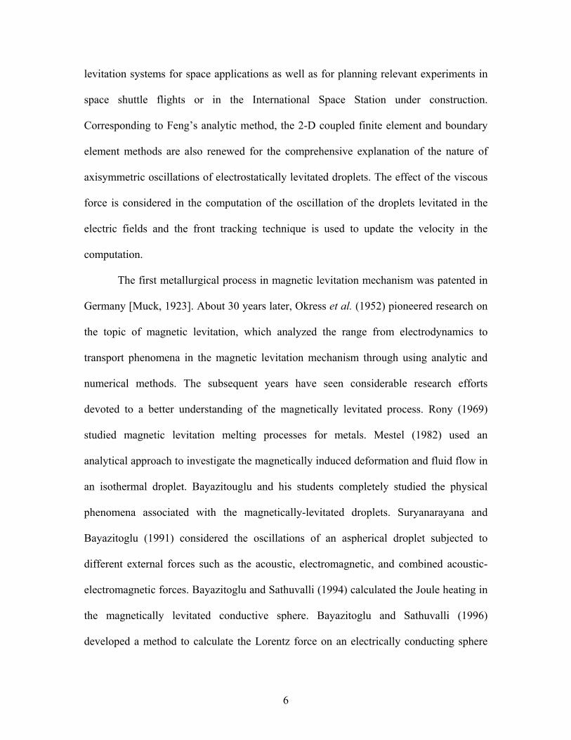
The first metallurgical process in magnetic levitation mechanism was patented in

Germany [Muck, 1923]. About 30 years later, Okress et al. (1952) pioneered research on

the topic of magnetic levitation, which analyzed the range from electrodynamics to

transport phenomena in the magnetic levitation mechanism through using analytic and

numerical methods. The subsequent years have seen considerable research efforts

devoted to a better understanding of the magnetically levitated process. Rony (1969)

studied magnetic levitation melting processes for metals. Mestel (1982) used an

analytical approach to investigate the magnetically induced deformation and fluid flow in

an isothermal droplet. Bayazitouglu and his students completely studied the physical

phenomena associated with the magnetically-levitated droplets. Suryanarayana and

Bayazitoglu (1991) considered the oscillations of an aspherical droplet subjected to

different external forces such as the acoustic, electromagnetic, and combined acoustic-

electromagnetic forces. Bayazitoglu and Sathuvalli (1994) calculated the Joule heating in

the magnetically levitated conductive sphere. Bayazitoglu and Sathuvalli (1996)

developed a method to calculate the Lorentz force on an electrically conducting sphere

7

placed in an arbitrary sinusoidally alternating magnetic field. In their research, they used

multipole expansion to express the vector potential of the external magnetic field in terms

of the source. The external magnetic field was calculated by using a gradient formula.

Lohofer (1989) solved the underlying quasistatic Maxwell equations using analytic

expansion in spherical harmonics and Bessel functions. The power absorption and lifting

force in the conducting sphere exposed to the external, time-varying magnetic fields were

analytically calculated. In his previous publication (1993), he studied the force and torque

of an electromagnetically levitated metal sphere. Lohofer (1994) also analyzed the

magnetization and impedance of an electrically conducting sphere, which was inductively

coupled with an arbitrary, sinusoidally alternating current density distribution. Li (1993)

presented an analytical study of the electromagnetic and thermal phenomena in magnetic

levitation. Analysis showed that the power input, the lifting forces and the temperature

distributions, both global and local, were proportional to the square of input current. At

high frequency limit, the total power input and the temperature were proportional to the

square root of applied frequency and inversely proportional to the square root of

electrical conductivity. Li (1994a) reported an analytic study of magnetohydrodynamic

phenomena in electromagnetic levitation processes. In his study, the flow was treated as a

Stokes flow, and the turbulence in the system was accounted for by using a constant eddy

viscosity model. Calculated results illustrated that the flow field was characterized by two

toroidal recirculating loops, and was strongly correlated to the distribution of the curl of

the force field, which in turn depended on the coil placement. Li (1994b) further analyzed

the transient electrodynamics and fluid flow phenomena in a magnetically-levitated liquid

sphere.

8

The numerical models were originally developed by Zong, et al. (1992, 1993). In

their formulation the electromagnetic force field was calculated using a modification of

the volume integral method and these results were then combined with the FIDAP code

to calculate the steady state melt velocities and the transient evolution of the velocity and

the temperature fields when the heating current is switched off. All these numerical

studies focused on the isothermal melt flow and the detailed temperature effects were not

considered. Later on, Song and Li (1998a, 1998b, 1999a) further developed the numerical

models to couple the boundary and finite element methods. They addressed the research

on how the free surface deformation would affect the Joule heating distribution and hence

the temperature field in a droplet in magnetic levitation systems. Their study indicated

that a more accurate assessment must include free surface deformation and sample

position in the levitation potential well. Ai and Li (2004) addressed fluid flow instabilities

and flow transition to turbulence chaotic motions through numerical analysis and

turbulence in magnetic levitated droplets through numerical simulations. Their results

indicated that both turbulence kinetic energy and dissipations attained finite values along

the free surface of the droplets.

Although a lot of study has been implemented using the various methods such as

the analytic, experimental, and numerical methods, many important issues remain still

unknown, for example, the movement of droplets in the magnetic levitation mechanism.

Only, Enokizono, et al., (1995) investigated the simulation of the movement of metal in

the levitation-melting apparatus. However, nodal-based elements are used in their

boundary and finite element methods so that the spurious solution occurred. While

various approaches may be applied to alleviate the problem, the approach in the present

9

study uses the edge elements to satisfy the divergence-free condition so as to eliminate

the spurious solution. Consequently, both the finite element and boundary element

interpolations are edge-based to ensure the finite and boundary element method

compatibility. While possible in theory, the numerical implementation of an edge-based

FEM/BEM method does not appear to have been attempted for the solution of

electromagnetic-heating-moving problems in general 3-D geometries.

1.3 Objectives of Present Research

The major objectives of this research are to develop 2-D and 3-D numerical models for

solving the electromagnetic, fluid flow, heat transfer, mass transfer and surface

deformation phenomena in electrostatic and magnetic levitation mechanism under the

microgravity conditions in order to provide information for the measurement of

thermophysical properties and the fundamental study of nucleation and crystal growth

phenomena. The numerical method can test the experimental results and predict the

multi-physical phenomena that can not be implemented by using the analytical and

experimental methods.

Various numerical studies are implemented in the electrostatically or magnetically

levitated droplets. The 2-D coupled boundary and finite elements with a WRM-based

algorithm are used to predict the free surface deformation with hydraulic effect and

without hydraulic effect. The 3-D Galerkin finite element method is used to solve the

Navier-Stokes and energy equations. The complex 3-D steady-state and transient

Marangoni convection and heat transfer in electrostatically levitated droplets are

10

investigated using the 3-D finite element model. The 3-D coupled boundary and finite

elements with edge elements are used to predict the droplet movement in the magnetic

levitation mechanism.

1.4 Scope of Present Research

In the present study, eight major sections are discussed. Chapter 2 lists the complete

mathematical statement of physical phenomena in the electrostatically and magnetically

levitated droplets. Chapter 3 presents the detail of the computational methodology, which

is used to solve governing equations and boundary conditions, as described in chapter 2.

Chapter 4 discusses the numerical results of free surface deformation, and the steady state

and transient 3-D Marangoni convection and heat transfer in electrostatically levitated

droplets. Chapter 5 analyzes the solute transport phenomena in electrostatically levitated

droplets under microgravity, based on the computational results of the free surface

deformation, full 3-D Marangoni convection in chapter 4. Chapter 6 presents the free

surface deformation and Marangoni convection in immiscible droplets positioned by an

electrostatic field and heated by laser beams under microgravity. Chapter 7 shows the

computed results of the oscillation of the electrostatically levitated droplet under

microgravity. Chapter 8 depicts the 3-D movement of the conducting droplet in the

magnetic levitation mechanism.

11

CHAPTER 2

PROBLEM STATEMENT

2.1 Electrostatically Levitated Droplets under Microgravity

Let us consider the problem as illustrated in Figure 2.1. An electrically conducting liquid

droplet is immersed in a uniform electrostatic field, which is generated by placing two

electrodes far apart (Figure 2.1a). By the principle of electrostatics, a constant potential is

established on the surface of the droplet, and surface electric charges are induced so that

the electric field inside the droplet is zero. The charge distribution is non-uniform along

the surface and, when combined with a self-induced electric field local to the charges,

results in a non-uniform electric surface force acting in the outnormal direction [Reitz,

1979]. This normal force combines with other surface forces to define the equilibrium

shape of the droplet. The internal and tangential surface Maxwell stresses are both zero

because the electric potential is constant everywhere inside the droplet by the Gauss law

and thus there will be no convection resulting from the electric origin. Laser beams are

applied to melt the sample and/or heat it up to a designated temperature. Figure 2.1b

shows a heating arrangement with two laser beams directed at two poles. Various other

laser beam arrangements are also considered in this study, including single beam, dual

beam, tetrahedral and hexahedral beams. The heating will result in a non-uniform

temperature distribution inside the droplet and cause convection if the surface tension of

the liquid varies with the surface temperature, as for most metallic and semiconductor

melts. Since the laser heating applied here is not necessarily axisymmetric, the surface

12

tension driven flows are bound to be three-dimensional. As shown later, very complex 3-

D flow structures and temperature distributions are developed in a droplet for some

heating conditions. One important objective of this present study is to develop an

understanding of these complex transport phenomena under both steady and transient

conditions, which each have specific applications for space materials processing and

thermophysical property measurements.

13

(a)

Q0

Q0

(b)

Figure 2.1 Schematic representation of a positively charged melt droplet levitated in an

electrostatic field: (a) levitation mechanism and (b) two-laser-beam heating arrangement.

14

2.1.1 Governing equations and boundary conditions for the thermal convection in the

electrostatically levitated droplet under microgravity

A complete description of the electrically induced surface deformation and thermally

induced fluid flow phenomena in a droplet requires the solution of the coupled Maxwell

and Navier-Stokes equations, along with the energy balance equation. However, for metal

and semiconductor melts, the electric Reynolds number, (ε0/σ)Vmax/a, is on an order of

10-16, which suggests that the convective transport of surface charges (or electric field)

may be neglected and the electric field distribution can be calculated as if the liquid

droplet were solid [James, 1981]. With this, the Maxwell equation is simplified to a

partial differential equation governing the distribution of the electric field outside the

droplet. The buoyancy effects being neglected for microgravity applications, the

equations for the electric, fluid flow and thermal fields may be written as follows,

02 =Φ∇ 2Ω∈ (2.1)

0u =⋅∇ 1Ω∈ (2.2)

( )Tpt

)u(uuuu∇+∇⋅∇+−∇=∇⋅+

∂∂ ηρρ 1Ω∈ (2.3)

TkTCtTC pp ∇⋅∇=∇⋅+

∂∂ uρρ 1Ω∈ (2.4)

where 1Ω and 2Ω refer to the regions inside the droplet and outside the droplet

respectively. Φ is the electric potential, u the velocity, p the pressure, and T the

temperature. Also, η is the molecular viscosity, ρ the density, pC heat capacity, and k

15

thermal conductivity. The solution of above electric field, fluid flow and heat transfer

equations may be obtained by applying the appropriate boundary conditions, which are

stated below,

0Φ=Φ 21 Ω∩Ω∈ (2.5)

eσε −=Φ∇⋅n0 21 Ω∩Ω∈ (2.6)

Qdsdse =Φ∇⋅−= ∫∫∫∫ΩΩ

n11

0∂∂

εσ 21 Ω∩Ω∈ (2.7)

θcos0RE−=Φ ∞→R (2.8)

( ) 22 /44 ˆ ll arols eQTTTk −

∞ ⋅+−=∇⋅− rnn εσ 21 Ω∩Ω∈ (2.9)

0=⋅ nu 21 Ω∩Ω∈ (2.10)

γσ HK E 2=⋅⋅−+⋅⋅ nTnnn 21 Ω∩Ω∈ (2.11)

TdTd

∇⋅=⋅⋅ tnt γσ 21 Ω∩Ω∈ (2.12)

01

VdV =∫Ω 21 Ω∩Ω∈ (2.13)

czdVz =∫Ω1 21 Ω∩Ω∈ (2.14)

In the above, Eq. (2.6) is the jump condition for the electric field along the droplet

surface, a manifestation of a well known fact that charges are distributed only on the

surface of a conducting body. Eq. (2.8) describes the electric potential condition at

infinity. The law of charge conservation is described by Eq. (2.7), where Q is the total

free charge applied on the droplet, which is zero for the problem under consideration for

16

microgravity applications. In Eq. (2.9), the absorption coefficient is factored into Qo and

lr the unit vector of laser beam pointing outward from the origin of the laser, i.e.,

0ˆ ≤⋅ lrn . Eq. (2.11) describes the balance of the hydrodynamic, Maxwell and surface

tension stresses along the normal direction, which determines the shape of the droplet.

The last equation represents the fact that the flow along the surface of the droplet is

induced by surface tension force if it is a function of temperature. The constraints of the

volume conservation (Eq. (2.13)) and the center of the mass (Eq. (2.14)) of the

electrostatically levitated droplet are needed to determine the shape and position of the

droplet.

2.1.2 Governing equations and boundary conditions for the mass transfer in the

electrostatically levitated droplet under microgravity

For some applications such as impurity doping and diffusivity measurements [Johnson,

2002], foreign material may be continuously introduced on the surface once flow is

established. A strong recirculation in the droplet will likely play an important role in

transporting the impurity from the surface to the inside, as sketched in Figure 2.2. A

quantitative assessment of the convection effect on the impurity transport in the droplet

will be made in this study for the conditions of relevance to diffusion coefficient

measurements [Johnson, 2002].

The deformation, fluid flow and heat transfer is calculated from eq. (2.1) to eq.

(2.14). Combined with the above equations, the governing equation for mass transfer may

be written as follows,

17

CDCtC

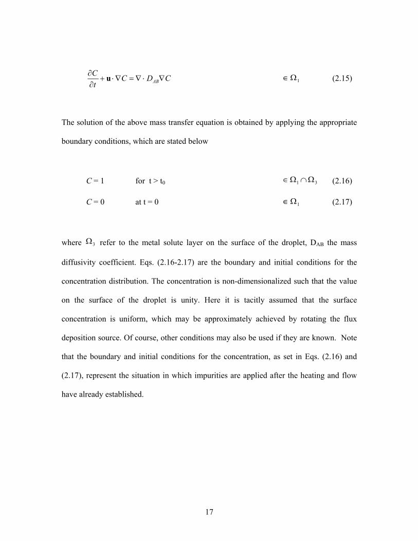
AB∇⋅∇=∇⋅+∂∂ u 1Ω∈ (2.15)

The solution of the above mass transfer equation is obtained by applying the appropriate

boundary conditions, which are stated below

C = 1 for t > t0 31 Ω∩Ω∈ (2.16)

C = 0 at t = 0 1Ω∈ (2.17)

where 3Ω refer to the metal solute layer on the surface of the droplet, DAB the mass

diffusivity coefficient. Eqs. (2.16-2.17) are the boundary and initial conditions for the

concentration distribution. The concentration is non-dimensionalized such that the value

on the surface of the droplet is unity. Here it is tacitly assumed that the surface

concentration is uniform, which may be approximately achieved by rotating the flux

deposition source. Of course, other conditions may also be used if they are known. Note

that the boundary and initial conditions for the concentration, as set in Eqs. (2.16) and

(2.17), represent the situation in which impurities are applied after the heating and flow

have already established.

18

Figure 2.2 Schematic representation of solute transport in the outer layer into the heated

droplet. Note that the solute concentration at the surface is dilute but kept at a constant.

2.1.3 Governing equations and boundary conditions for the thermal convection in the

electrostatically levitated droplet comprised of immiscible liquid metals under

microgravity

A positively charged droplet comprised of immiscible liquid metals levitated in an

electrostatic field is also investigated in the present study. The numerical model is

capable of providing the significant information about the internal convection in the

droplet, which is useful for the thermophysical measurement for the immiscible liquid

metals. Like the equations described in section 2.1.1, a complete description of the

Trace of velocity

Metal solute layer

solvent (droplet)

Trace of mass diffusion

19

electrically induced surface deformation and thermally induced fluid flow phenomena in

a droplet comprised of immiscible liquid metals requires the solution of the coupled

Maxwell and Navier-Stokes equations, along with the energy balance equation in

different regions. The buoyancy effects being neglected for microgravity applications, the

equations for the electric, fluid flow and thermal fields may be written as follows,

02 =Φ∇ 2Ω∈ (2.18)

0=⋅∇ ju 31 Ω∪Ω∈ (2.19)

( )Tjjjjjj

j pt

)( uuuuu

∇+∇⋅∇+−∇=∇⋅+∂

∂ηρρ 31 Ω∪Ω∈ (2.20)

jjjjpjj

jpj TkTCt

TC

j∇⋅∇=∇⋅+

∂

∂uρρ 31 Ω∪Ω∈ (2.21)

where j (= 1, 3) with the subscript 1 refers to the outer layer of the droplet and 3 to the

inner layer. The solution of above electric field, fluid flow and heat transfer equations

may be obtained by applying the appropriate boundary conditions, which are stated

below,

0Φ=Φ 21 Ω∩Ω∈ (2.22)

eσε −=Φ∇⋅10n 21 Ω∩Ω∈ (2.23)

Qdsdse =Φ∇⋅−= ∫∫∫∫Ω∂∩ΩΩ∂∩Ω

n2121

0∂∂

εσ 21 Ω∩Ω∈ (2.24)

θcos0RE−=Φ ∞→R (2.25)

20

( ) 22 /1

44111 ˆ ll ar

ols eQTTTk −∞ ⋅+−=∇⋅− rnn εσ 21 Ω∩Ω∈ (2.26)

01 =⋅nu 21 Ω∩Ω∈ (2.27)

γσ HK E 211111 =⋅⋅−+⋅⋅ nTnnn 21 Ω∩Ω∈ (2.28)

11111 TdTd

∇⋅=⋅⋅ tnt γσ 21 Ω∩Ω∈ (2.29)

31 uu = 31 Ω∩Ω∈ (2.30)

31 TT = 31 Ω∩Ω∈ (2.31)

3313333 2 γσσ H=⋅⋅−⋅⋅ nnnn 31 Ω∩Ω∈ (2.32)

TdTd

∇⋅=⋅⋅−⋅⋅ 33

313333 tntnt γσσ 31 Ω∩Ω∈ (2.33)

031

VdV =∫ Ω+Ω 31 Ω∪Ω∈ (2.34)

czdVz =∫ Ω+Ω 31

31 Ω∪Ω∈ (2.35)

In the above, eqs. (2.22-2.29, 2.34-2.35) have the same formulation like that in section

2.1.1 except that they are calculated in the droplet comprised of the immiscible metals.

Eqs. (2.30-2.31) respectively present that the velocity and temperature are the same on

the surface between the immiscible liquid metals. The normal and tangential stress

balance is represented by Eqs. (2.32-2.33)

It is noted that in the above formulations, the effect of surrounding gas is omitted.

The liquid droplet is generally processed under a vacuum condition, although recently

attempts have been made to process in an inert gas environment. For the latter case, it is

21

estimated that the surrounding inert gas contributes about 3% or less to the Marangoni

convection.

2.1.4 Governing equations and boundary conditions for the computation of the oscillation

of the electrostatically levitated droplet under microgravity

In the study of the oscillation of electrostatically levitated droplets under microgravity,

Eqs. (2.1-2.3) are the governing equations. Parts of the boundary conditions may be

expressed in Eqs. (2.5-2.8), Eq. (2.11), and Eqs. (2.13-2.14). Also one additional

boundary condition is needed, as shown below.

0)( =⋅− nuu s 21 Ω∩Ω∈ (2.36)

where us is surface velocity. Along the free surface of the droplet, eq. (2.36) results in the

following boundary condition:

0XudtdX

=∇⋅+ 21 Ω∩Ω∈ (2.37)

with X being the free surface coordinates.

22

2.2 Magnetically Levitated Droplets under Microgravity

Figure 2.3 shows the TEMPUS device in use [Song, 1998a, 1998b, 1999a]. The system

consists of two types of coils: (1) the inner four current loops (or heating coils) for

sample heating and melting, and (2) the outer eight loops (or positioning coils) for sample

positioning in space. During the operation, AC currents flow through these coils to

generate an appropriate magnetic field. In magnetic levitation, eddy currents are induced

in the sample and the dot product of eddy currents generates the Joule heating for the

melting of the sample. These eddy currents also interact with the applied and induced

magnetic fields to produce the Lorentz force in the sample. At present, we investigate the

effect of the Lorentz force on the metal’s movement in the magnetic levitation

mechanism.

13.5

9.5

10

4

4

Figure 2.3 Schematic representation of magnetic levitation System

23

2.2.1 Governing equations and boundary conditions for the computation of the

electromagnetic field

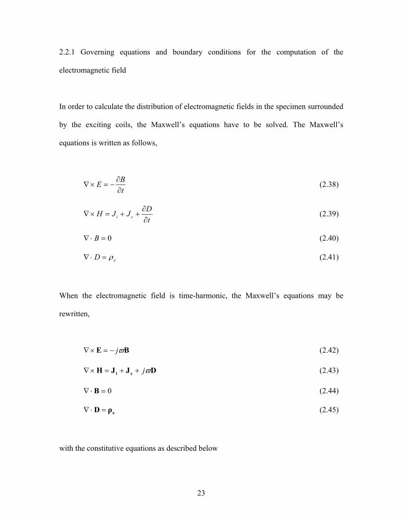
In order to calculate the distribution of electromagnetic fields in the specimen surrounded

by the exciting coils, the Maxwell’s equations have to be solved. The Maxwell’s

equations is written as follows,

tBE

∂∂

−=×∇ (2.38)

tDJJH ci ∂

∂++=×∇ (2.39)

0=⋅∇ B (2.40)

eD ρ=⋅∇ (2.41)

When the electromagnetic field is time-harmonic, the Maxwell’s equations may be

rewritten,

BE ϖj−=×∇ (2.42)

DJJH ci ϖj++=×∇ (2.43)

0=⋅∇ B (2.44)

eρD =⋅∇ (2.45)

with the constitutive equations as described below

24

ED ε= ED ε= (2.46)

HB µ= HB µ= (2.47)

EJc σ= EJc σ= (2.48)

and the general boundary conditions described as follow,

0)( 12 =−× EEn 0)( 12 =−× EEn (2.49)

eqDDn =−⋅ )( 12 eqn =−⋅ )( 12 DD (2.50)

where E (E) is the electric field intensity, H (H) the magnetic field intensity, D (D) the

electric flux density, B (B) the magnetic flux density, Ji (Ji) impressed electric current

density, Jc (Jc) conduction electric current density, ρe (ρe) electric charge density, ε

permittivity, µ permeability, and σ conductivity.

However, Maxwell’s equations are coupled partial differential equations, which

have more than one unknown variables. Therefore, the vector wave equation derived

from the Maxwell’s equations combined with the energy equation is taken as the

governing equations to simulate the microwave heating problems. With the analysis

above, the equations for the electric and thermal fields may be written as follows

icr

j JEE ωµµεωµ

−=−×∇×∇ 21 (2.51)

25

In the above, Ji is an impressed or source current, and εc (=ε-jσ/ω) results from the

combination of the induced current (σE) and displacement current (jωD). The appropriate

boundary conditions are stated below.

2221111

ˆˆ1 EnUUEn ×∇×==−=×∇×−rµ

21 Ω∩Ω∈ (2.52)

where Ω1 and Ω2 are the FEM domain, BEM domain respectively. 1n is outnormal from

the FE region, and 2n is outnormal from the BE region.

2.2.2 Governing equations and boundary conditions for the computation of the movement

of the droplet in the magnetic levitation mechanism

After the computation of the electromagnetic field, the time-averaged electromagnetic

force induced in the sphere which is responsible for levitation as well as for fluid motion,

is the cross product of induced current and the complex conjugate of the magnetic field,

)B(J21F ∗×= Re (2.53)

dVV

⋅= ∫ FFtotal (2.54)

where i is the element number. As the levitating motion, we considered the translation.

Therefore, the translation equations are introduced into this analysis. The Leap Frog

26

Algorithm is used. This algorithm evaluates the velocities at half-integer time steps and

uses these velocities to compute new positions.

t

ss nn

∆−

≡++ 1

21n

v (2.55)

tss nn

∆−

≡−− 1

21n

v (2.56)

So we can derive the new position, based on the old position and velocity:

21

n1n tvss++ ∆+=

n (2.57)

From the Verlet algorithm, we have the following expression for velocity:

n21n

21n

avv t∆+=++

(2.58)

m/Fa totaln n= (2.59)

where a is the acceleration, m is the weight of the metal, ∆t the width of time step, v the

velocity at center of the metal and s the position vector. The fluid flow and temperature

distribution may also be calculated at every time step.

After the time-averaged electromagnetic force is calculated, the torque with

respect to the axis may be written as follows,

27

tiitiN FR ×= (2.60)

∑=

=1

totalNi

tiN (2.61)

The rotating moving equations at every time step are given by,

nn ωωω ∆+=+ n1 (2.62)

nn θθθ ∆+=+ n1 (2.63)

with

mn I∆t /Ntotal=∆ω (2.64)

)2/(N 2total m

nn I∆tt +∆=∆ ωθ (2.65)

where Ri is the radius vector drawn from center to surface of a sphere metal, ω the

angular velocity, θ the rotational angle, and mI the moment of inertia. In the present

study, the droplet is assumed to be spherical without considering the deformation of the

droplet. Therefore, the moment of inertia mI may be written as,

2mR)5/2(=mI

where m is the weight of the droplet, R the radius of the spherical droplet.

28

CHAPTER 3

NUMERICAL SOLUTIONS

In the present study of the droplet in electric levitation mechanism, the electric field is

calculated by the boundary element method (BEM) and the shape deformation by the

Weighted Residuals method. The numerical model for the transport phenomena is

developed based on the Galerkin finite element solution (FEM) of the Navier-Stoke

equations, the energy balance equation and the mass transport equation. The

computational models developed here enable the prediction of the electric field

distribution, electric pressure distribution along the surface of a droplet, droplet shapes,

the internal fluid flow, thermal and solute distributions in electrostatically positioned

droplets. For the movement of the droplet in the magnetic levitation mechanism, the

numerical models are implemented using the boundary and finite element method with

edge elements to calculate the electromagnetic fields in the conducting droplets. And then

the force is calculated by the integral volume of the droplet, which is used in the dynamic

equations to solve the movement of the droplet. From now on, unless otherwise indicated,

the FEM and BEM respectively represent the finite element method and boundary

element method.

3.1 An Introduction to the FEM and BEM

Let’s begin with an introductory definition of the finite element method (FEM): The

FEM is a computer-aided mathematical technique for obtaining approximate numerical

29

solution of the physical phenomena subject to the external influence. The FEM originally

arises from the area of solid mechanics (elasticity, plasticity, statics, and dynamics).

Applications to date have been expanded to the broad field of engineering science such as

heat transfer (conduction, convection and radiation), fluid mechanics (inviscid or viscous,

compressible or incompressible), acoustics, and electromagnetics.

The basic idea of the FEM is summarized as follows: (a). the domain of the

problem is partitioned into smaller regions, called elements, (b). in each element the

governing equations are transformed into algebraic equations, called the element

equations, (c). the terms in the element equations are numerically evaluated for each

element in the mesh, (d). the resulting numbers are assembled into a much larger set of

algebraic equations, called the system equations, (e). the system equations are solved by

using the numerical technique on computer, (f). the final operation displays the solutions

to tabular, graphical, or pictorial form.

There are two types of optimizing route leading to the FEM formulation: (a).

methods of weighted residuals (MWR), which are applicable when the governing

equations are differential equations, (b). variational method (VM), which is applicable

when the governing equations are variational (integral) equations. The MWR seek to

minimize the residue in the differential equations. There are four basic types in the MWR

route: (a). the collocation method, (b). the subdomain method, (c). the least-squares

method, (d). the Galerkin method. The variational principles try to minimize some

physical quantity, such as energy.

Over recent decades, the boundary element method (BEM) has received much

attention from researchers and has become an important technique in the computational

30

solution of a number of physical problems. It is based on the boundary integral equation

and the methods of weighted residuals, where the Green’s function of the corresponding

governing equation is chosen as the trial function. The advantages in the boundary

element method arise from the fact that only the boundary of the domain requires sub-

division. The method is particularly suited to solve problems with boundaries at infinity.

The method includes the following steps: (a). the surface of the domain of the problem is

partitioned into smaller regions, called boundary element, (b). the Green’s function is

selected as the trial function and the governing equations are transformed into algebraic

equations on the boundary elements, (c). the final element matrix is assembled over

element by element, (d). the system equations are solved by using the numerical

technique on computer.

3.2 Computation of the Deformation of the Droplet in the Electric Levitation

Mechanism

As stated in chapter 2, for practical applications, droplet deformation is essentially

axisymmetric and viscous forces make a negligible contribution. Thus, the electric and

droplet deformation calculations may be decoupled from the thermal and fluid

calculations. The procedures for the computation of electrically induced droplet

deformation are detailed in our previous publications [Huo, 2004a, 2004b, 2005a]. Since

the electric field inside the droplet is zero, only the potential distribution outside needs to

be solved for.

31

3.2.1 Computation of the distribution of the electric potential

We now apply the BEM to determine the scalar electric potential in the exterior region of

the droplet levitated in the electric field. We are seeking an approximate solution to the

problem governed by

02 =Φ∇ 2Ω∈ (3.1)

which is the same as Eq. (2.1). The error introduced by replacing Φ by an approximate

solution can be minimized by writing the following weighted residual statement:

∫∫ ∫ΓΩ Γ

ΓΦ−Γ=ΩΦ∇ )(),()()(),()()(),()( *2

2

rdrrqrrdrrGrqrdrrGr iii (3.2)

where G is interpreted as a weighting function and

)(

),(),(*

rnrrGrrq i

i ∂∂

= (3.3)

The integration of Eq. (3.3) by parts with respect to xi gives

∫∫ ∫ΓΩ Γ

ΓΦ+Γ−=Ω∂

∂∂Φ∂

− )(),()()(),()()()(),(

)()( *

2

rdrrqrrdrrGrqrdrxrrG

rxr

iii

i

i

(3.4)

32

where i= 1, 2, 3 and Einstein’s summation convection for repeated indices is implied.

Integrating by parts once more,

∫∫ ∫ΓΩ Γ

ΓΦ+Γ−=Ω∇ )(),()()(),()()()(),( *2

2

rdrrqrrdrrGrqrdrurrG iii (3.5)

Assuming G to be fundamental solution to Laplace’s equations means that

),(2),(2 rrrrG ii απδ−=∇ (3.6)

where δ is the Dirac Delta function. Here G is the Green’s function. Substituting Eq.

(3.6) into Eq. (3.5) gives

∫∫ΓΓ

Γ=ΓΦ+Φ )(),()()(),()()(2 * rdrrGrqrdrrqrr iiiαπ (3.7)

So, taking the point ri to the boundary and accounting for the jump of the left-hand side

integral in Eq. (3.7) yields the boundary integral equation

∫∫ΓΓ

Γ=ΓΦ+Φ )(),()()(),()()()( * rdrrGrqrdrrqrrrC iiii (3.8)

After some transformation, we can get the final form used for the BEM simulation.

33

ΓΦ∇⋅+ΓΦ∇⋅

=Γ∇⋅Φ+Γ∇⋅Φ+Φ

∫∫

∫∫

ΩΩ

ΩΩ

drGdrG

rdGrdGrrC ii

22

22

)'()'(

)(')(')(')(

∂∂

∂∂

nn

nn

(3.9)

where

⎪⎪⎪

⎩

⎪⎪⎪

⎨

⎧

−−

=

;2

2

;21;1

)(

21

πββπ

irC

and Φ’ = Φ + Ercosθ, ∂Ω2 designates the surface of the droplet and 2Ω∂ denotes the

boundary at infinity. The Green function, G, and its normal derivative are calculated by

the following expressions written for a cylindrical coordinate system [Jackson, 1975].

( ) ( )

)(4),(22

κKzzrr

rrGii

i−++

= (3.10)

( ) ( )

( ) ( )[ ]( ) ( )

⎪⎪⎭

⎪⎪⎬

⎫

⎪⎪⎩

⎪⎪⎨

⎧

−+−−+−

−−

−++=

)()()(

24

22

22κ

κκ

∂∂

Ezzrr

zznrrn

KEr

n

zzrrnG

ii

izir

r

ii

(3.11)

where κ is the geometric parameter calculated by

when ri lies inside domain

when ri lies on a smooth domain

when ri lies on a nonsmooth domain

34

222

)()(4

zzrrrr

ii

i

−++=κ (3.12)

The function G and Φ’ have the following asymptotic properties,

)(),(' 2−≈Φ RORri , )(),(' 3−≈Φ RORrn i∂

∂ as ∞→R (3.13)

)(),( 2−≈ RORrG i , )(),( 3−≈ RORrnG

i∂∂ as ∞→R (3.14)

Also dΓ = R(θ) dθ. Thus, the two integrals each approach zero as R → ∞ ,

0)('2

→Γ∇⋅Φ∫Ω∂

rdGn and 0)'(2

→ΓΦ∇⋅∫Ω∂

rdG n as ∞→R (3.15)

Thus, Eq. (3.9) simplifies to a boundary integral that involves only the surface of the

droplet, ∂Ω2. Following the standard boundary element discretization, noticing that the

potential on the surface is a constant and substituting Φ = Φ’ - Ercosθ into the resultant

equation, one obtains the final matrix form for the unknowns on the surface of the

droplet,

zEnzE

nHGGH −

⎭⎬⎫

⎩⎨⎧+

⎭⎬⎫

⎩⎨⎧ Φ

−=Φ∂∂

∂∂

0 (3.16)

35

where H and G are the coefficient matrices involving the integration of ∂G/∂n and G over

a boundary element. To complete the solution, Eq. (2.8) is discretized and solved along

with the above equation to obtain the surface distribution of ∂Φ/∂n and the constant Φ0.

3.2.2 Computation of the deformation of the droplet

The study of the free surface deformation of the electrostatically levitated droplet plays

an important role in the future computation of the fluid flow and temperature distribution.

In particular, it can affect the ratio of the radiation when the laser beams are switch off.

For the electrostatically levitated droplet, its shape is determined by the hydrostatic

pressure, the electrostatic pressure and the surface tension of the liquid, as shown in Eq.

(2.11). The normal stress balance equation (Eq. (2.11)) along the droplet surface is solved

using the Weighted Residuals method. Written in a spherical coordinate system, which is

more convenient for the calculations.

mPaBrKrr

rrdd

rrrr

r γθθ

θθ

θθ

θ

θ

θ −−−=+

−+

+ cos)]sin(sin)2([sin1

2222

22

2 (3.17)

where a is the radius of the undeformed sphere, r the non-dimensionalized radial

coordinate, γ/0aPK = , γρ /2gaB = , and 2/)( 20 Φ∇⋅−= nPm ε . The weighted residual

method may be applied to solve Eq. (3.17) once the potential field distributions are

known. The solution of Eq. (3.17) by the weighted residual method is constructed by

integrating Eq. (3.17) with a weighting function ψ along the droplet surface,

36

0cos

)]sin(sin)2([sin1

1

2222

22

2

=

⎪⎪⎭

⎪⎪⎬

⎫

⎪⎪⎩

⎪⎪⎨

⎧

++

++

−+

+

∫Ω∂

dsPaBrK

rrrr

dd

rrrr

ri

m

ψ

γθ

θθ

θθ

θ

θ

θ

θ

(3.18)

Where θθ ddrr /= . Integrating by parts, the weighted residuals approach leads to the

following integral representation of the force equilibrium along the surface.

( )0sin

cos

2

02

22

22

=

⎪⎪⎪

⎭

⎪⎪⎪

⎬

⎫

⎪⎪⎪

⎩

⎪⎪⎪

⎨

⎧

⎟⎟⎠

⎞⎜⎜⎝

⎛−+

++

++

∫ θθ

γθψ

ψθψ

π

θ

θθ

d

PaBrKr

rr

rrddrr

mi

ii

(3.19)

The variables r and rθ are calculated by

i

Ne

iirr ∑

=

=1ψ and ∑

=

=Ne

i

ii d

dddrr

1 θζ

ζψ

θ (3.20)

The constraints of the volume conservation and the center of the mass of the levitated

sphere are needed to determine the shape and position of the droplet. In dimensionless

form, the two constraints are expressed as

2sin1

0

33

=∫ θθπ

drad

(3.21)

37

czdrad

=∫ θθθπ

sincos83

0

43

(3.22)

where zc is the center of mass. The free surface may be discretized into N elements and

Eqs. (3.20-3.22) are integrated numerically. The results may be arranged in the following

matrix form:

F=KX (3.23)

where

⎥⎥⎥⎥⎥⎥⎥⎥⎥⎥⎥

⎦

⎤

⎢⎢⎢⎢⎢⎢⎢⎢⎢⎢⎢

⎣

⎡

−⋅⋅⋅⋅

⋅⋅⋅⋅⋅⋅⋅⋅

=

−

−

−

−−−−−−

1121

121

,1,

1,11,12,1

23,22,21,2

12,11,1

nn

nn

nnnnn

nnnnnnn

ccccbbbb

baabaaa

baaabaa

K

⎥⎥⎥⎥⎥⎥⎥⎥⎥⎥⎥

⎦

⎤

⎢⎢⎢⎢⎢⎢⎢⎢⎢⎢⎢

⎣

⎡

⋅⋅

=−

c

n

n

zKr

r

rr

1

2

1

X

⎥⎥⎥⎥⎥⎥⎥⎥⎥⎥⎥

⎦

⎤

⎢⎢⎢⎢⎢⎢⎢⎢⎢⎢⎢

⎣

⎡

⋅⋅

=−

02

1

2

1

n

n

FF

FF

F (3.24)

where jia , , jb , jc and jF are calculated by

38

ξθ

ξθ

γψψ

ξθ

ξ

ξξψ

ψξ

ψξξ

θψψ

d

ddaPr

ddr

ddr

ddr

dd

dd

ddr

ddr

a

mji

jj

jji

ji sin

||

)()(

))(2[

1

1

22

2

, ∫−

⎪⎪⎪

⎭

⎪⎪⎪

⎬

⎫

⎪⎪⎪

⎩

⎪⎪⎪

⎨

⎧

++

++

= (3.25)

ξξθθψ d

ddrb ii ||sin

1

1

2∫−

= (3.26)

ξξθθθψ d

ddrc jj ||sincos

83 1

1

3∫−

= (3.27)

ξξθθθψ d

ddBrF ii ||sincos

1

1

3∫−

−= (3.28)

3.3 Computation of Thermal and Fluid Flow Fields

With the droplet shape known, the momentum and energy equations for the thermal and

fluid flow fields along with the boundary conditions may be solved using the Galerkin

finite element method. Both the transient and steady-state temperature and fluid flow

fields are calculated in the present study.

3.3.1 Computation of thermal and fluid flow fields in a single-phrase droplet

In essence, the computational domain is first divided into small elements. With each

element, the dependent variable u, P and T are interpolated by shape functions φ , ψ and

θ,

39

)(),()(),()(),(

ttxTttxPttx

T

T

iTi

TPUu

θ

ψ

φ

=

=

=

(3.29)

where the iU , )(tP and T are column vectors of element nodal point unknowns.

Substituting Eq. (3.29) into the governing Eqs. (2.2-2.4), we get the residuals R1,

R2 and R3 which represent the momentum, mass convection and energy equations

respectively. The Galerkin form of the Method of Weighted Residuals seeks to reduce

these errors to zero, and the shape functions are chosen the same as the weighting

function. The governing equations for the fluid flow and heat transfer may be rewritten as

PdVUdVi Tp

iT )())((11

∫∫ ΩΩ−=∇⋅ ψψεφψ

) (3.30)

∫∫∫

∫∫∫

Ω∂

ΩΩ

ΩΩΩ

⋅⋅

=∇⋅∇⋅+∇⋅∇+

∇⋅−∇⋅+

1

11

111

)))((())((

))(()()(

dsin

UdVjiUdV

PdViUdVudt

dUdV

ji

Tii

T

φσ

φφηφφη

ψφφρφρφφ))

)

(3.31)

∫∫∫∫

Ω∂Ω

ΩΩ

−=∇⋅∇

+∇⋅+

11

11

)(

)()(

dsqTdVk

TdVuCdtdTdVC

TT

Tp

Tp

θθθ

θθρθθρ (3.32)

Once the form of shape functions is specified, the integral defined in the above equations

can be expressed by the matrix equation. The momentum and energy equations may be

combined into a single global matrix equation,

40

⎥⎥⎥

⎦

⎤

⎢⎢⎢

⎣

⎡=

⎥⎥⎥

⎦

⎤

⎢⎢⎢

⎣

⎡

⎥⎥⎥

⎦

⎤

⎢⎢⎢

⎣

⎡

+−

−++

⎥⎥⎥

⎦

⎤

⎢⎢⎢

⎣

⎡

⎥⎥⎥

⎦

⎤

⎢⎢⎢

⎣

⎡

TTTT G

F

TPU

L(U)DC

BCKA(U)

TPU

N

MT 0

0000

0000000

&

&

&

(3.33)

The coefficient matrices above are defined by

∫Ω=

1

dVTp ψψM ; ∫Ω

=1

dVC TpT θθρN

∫Ω=

1

dVTφφM ; ∫Ω∇⋅=

1

ˆ dVj Tj φψC

∫Ω∇•∇=

1

dVk TT θθL ; ∫Ω

∇⋅=1

dVTφρφ u )U(A

∫Ω∇•=

1

dVC TpT θθρ u )U(D ; ∫ Ω∂

∇⋅∂∂

=1

dST

Tθγ tB

∫ Ω∂−=

1

G dsqTT θ ; ∫ Ω∂⋅=

nF

1

dsφτ

∫∫ ΩΩ∇⋅∇⋅+∇⋅∇=

11

)ˆ)(ˆ()( dVjidV Tij

Tij φφηδφφηK

where j=1, 2, 3. Note also that matrix B represents the surface tension effects on the fluid

motion. The assembled global matrix equations are stored in the skyline form and solved

using the Gaussian elimination method. The transient term is set to zero for steady-state

calculations, however.

3.3.2 Computation of thermal and fluid flow fields in a droplet of immiscible liquid

metals

41

The computation of thermal and fluid flow fields in the droplet of immiscible liquid

metals is very similar to that in the single-phrase droplet in section 3.3.1 except that the

calculation is carried out in two kinds of immiscible liquid metals. It is also necessary to

take account the effect of the surface tension on the surface between the immiscible

liquid metals, as presented by Eqs. (2.30-2.33). With each dependent variable u, P and T

in elements interpolated by the shape functions, φ , ψ and θ, The matrix form of the finite

element discretized equations for the thermal and fluid flow model may be written as

follows,

⎥⎥⎥

⎦

⎤

⎢⎢⎢

⎣

⎡=

⎥⎥⎥

⎦

⎤

⎢⎢⎢

⎣

⎡

⎥⎥⎥

⎦

⎤

⎢⎢⎢

⎣

⎡

+−

−++

⎥⎥⎥

⎦

⎤

⎢⎢⎢

⎣

⎡

⎥⎥⎥

⎦

⎤

⎢⎢⎢

⎣

⎡

TTTT G0F

TPU

L(U)D0000C0CKA(U)

TPU

N0000000M

T

&

&

&

(3.34)


∫Ω=

m

dVTφφM ; ∫Ω=

m

dVC TpT θθρN

∫Ω∇⋅∇=

m

dVk TT θθL ; ∫Ω

∇⋅=m

dVTm φρφ uUA )(

∫Ω∇⋅=

m

dVC TkpT θθρ uUD )( ; ∫ Ω∂∩Ω∂

−=21

dsqTT θG ;

∫Ω∇⋅=

m

dVj Tj φψˆC

∫∫ Ω∂∩Ω∂Ω∂∩Ω∂⋅−⋅+⋅⋅=

13

1

3121

)(ˆ ˆ dsjdsjj φσσφσ nnF

42

∫∫ ΩΩ∇⋅∇⋅+∇⋅∇=

mm

dVjidV Tij

Tij )ˆ)(ˆ()( φφηδφφηK

where m=1, 3. The assembled global matrix equations are stored in the skyline form and

solved using the Gaussian elimination method [Huo, 2004a]. The transient term is set to

zero for steady-state calculations, however.

3.3.3 Computation of mass transfer into a single-phrase droplet

With the thermal and fluid flow fields known, the equation governing the mass transfer

(Eq. (2.15)) is solved for the transient concentration distribution in the droplet [Huo,

2005a]. By the Galerkin finite element method, the variable C is interpolated by shape

function ξ ,

)(),( ttxC T Cξ= (3.35)

where the C(t) is column vectors of element nodal point unknowns. The matrix form of

the finite element discretized equation for the concentration field may be written as

follows,

0)( =++ CC CCC L(U)DN & (3.36)


43

∫Ω=

1

dVTC ξξN ; ∫Ω

∇⋅=1

dVTC ξξ u )U(D ; ∫Ω

∇⋅∇=1

dVTABC ξξϕL

Like the thermal and fluid flow calculations, the assembled global matrix equations are

stored in the skyline form and solved using the Gaussian elimination method [Huo,

2005a]. For this study, the implicit scheme is used to carry out the time matching

calculations.

3.3.4 Computational aspects in the thermal and fluid flow calculations

Modeling of 3-D surface tension driven flows on a curvilinear surface within the

framework of finite elements requires some tedious geometric treatment that involves

differential geometry operations and rotation of matrix in local coordinates at the surface

for the purpose of appropriately imposing velocity and surface stress boundary conditions

(Eqs.(2.10) and (2.12)). While treatment may vary depending on specific problems, our

approach to model the surface driven flow makes use of local surface coordinates and of

sharp edges with specified local coordinate system as well as consistent surface normals.

With reference to Fig. 3.1, a local coordinate system (η,ζ,n) is defined at a point on the

surface. Note that during calculations this local system may be (although not required)

chosen conveniently such that they are coincident with the normalized coordinate

systems for isoparemetric calculations at the element level. The xyz and ηζn coordinate

systems are related by the following coordinate transformation,

44

⎟⎟⎟⎟⎟⎟

⎠

⎞

⎜⎜⎜⎜⎜⎜

⎝

⎛

∂∂∂∂∂∂

⎥⎥⎥

⎦

⎤

⎢⎢⎢

⎣

⎡=

⎟⎟⎟⎟⎟⎟

⎠

⎞

⎜⎜⎜⎜⎜⎜

⎝

⎛

∂∂∂∂∂∂

=

⎟⎟⎟⎟⎟⎟⎟

⎠

⎞

⎜⎜⎜⎜⎜⎜⎜

⎝

⎛

∂∂

∂∂

∂∂

z

y

x

zyxzyxzyx

z

y

xJ

nnnn ,,,

,,,

,,,

][ ζζζ

ηηη

ζ

η

(3.37)

In constructing the Jacobian matrix, use has been made of the following differential

geometry relations,

^

,

^

,

^

,1 kzjyix ηηη ++=r , ^

,

^

,

^

,2 kzjyix ζζζ ++=r

( ) ( ) ^

,,,,

^

,,,,

^

,,,,

^

,

^

,

^

,21 )( kxyyxjxzzxiyzzykzjyix nnnn ζηζηζηζηζηζη −+−−−=++=×= rrr

The Jacobian matrix may be inverted analytically with the follow result,

[ ]⎥⎥⎥

⎦

⎤

⎢⎢⎢

⎣

⎡

−−−−−−−−−−−−

=−

ζηζηηηζζ

ζηζηηηζζ

ζηζηηηζζ

,,,,,,,,,,,,

,,,,,,,,,,,,

,,,,,,,,,,,,1

)()(

)(1

xyyxxyyxxyyxxzzxxzzxxzzxyzzyyzzyyzzy

JJ

nnnn

nnnn

nnnn

(3.38)

Furthermore, a shape (or any) function f(η,ζ) defined over the surface is a function of

(η,ζ) only and hence 0),( =∂∂ nf ζη . With these relations, one may then relate the

volume differential operator to the surface operator,

45

⎟⎟⎟⎟⎟⎟⎟

⎠

⎞

⎜⎜⎜⎜⎜⎜⎜

⎝

⎛

∂∂

∂∂

∂∂

=

⎟⎟⎟⎟⎟⎟

⎠

⎞

⎜⎜⎜⎜⎜⎜

⎝

⎛

∂∂∂∂∂∂

−

n

J

z

y

x

ζ

η1][ (3.39)

which may be written in the terminology of differential geometry [Weatherburn, 1930],

)(1)(1ˆˆˆ1212 ηζζη ∂

∂−

∂∂

+∂∂

−∂∂

=∂∂

+∂∂

+∂∂

=∇ FEH

FGH

kx

jx

ix

rr (3.40)

with 2,

2,

2,

21 ηηη zyxE ++== r , 2

,2,

2,

22 ζζζ zyxG ++== r , ζηζηζη ,,,,,,21 zzyyxxF ++=⋅= rr

and 22 FEGH −= . It is stressed that in Eq. (3.40), ( ηζ , ) is not necessarily orthogonal

so long as they are not collinear. This is important in that irregular quadrilateral surface

elements can be readily handled in 3-D finite element calculations presented here.

To perform the calculations, the consistent normal of the surface at node i is

required, which must satisfy the continuity equation [Engelman, 1982],

∫Ω ∂∂

=1

1 dVxn

n i

i

ix

φ , ∫Ω ∂∂

=1

1 dVyn

n i

i

iy

φ , ∫Ω ∂∂

=1

1 dVzn

n i

i

iz

φ (3.41)

where

⎥⎥⎦

⎤

⎢⎢⎣

⎡⎟⎠⎞

⎜⎝⎛

∂∂

+⎟⎟⎠

⎞⎜⎜⎝

⎛∂∂

+⎟⎠⎞

⎜⎝⎛

∂∂

= ∫∫∫ ΩΩΩ

222

111 zdV

ydV

xn iii

iφφφ

46

Note that the integration is carried over all the elements sharing node i. Once the normal

is known, the two tangential directions t1=( 111 ,, zyx ttt ) and t2=( 222 ,, zyx ttt ) can be easily

calculated using the cross product relations, t1= b x n, which b is an arbitrary space

vector such that b x n ≠ 0, and t2 = n x b. This ensures that the local coordinate system

defined by t1 x t2 x n forms an orthogonal triplet at any node (e.g. node i), a strict

condition different from that imposed on (η,ζ,n). The velocities defined in the t1 x t2 x n

system is now related to those in the xyz system through the following transformation,

⎟⎟⎟

⎠

⎞

⎜⎜⎜

⎝

⎛

n

t

t

UUU

1

2

= ⎥⎥⎥

⎦

⎤

⎢⎢⎢

⎣

⎡

zyx

zyx

zyx

nnntttttt

222

111

⎟⎟⎟

⎠

⎞

⎜⎜⎜

⎝

⎛

z

y

x

UUU

(3.42)

Note that the above transformation also applies to force vectors.

To calculate the surface tension contributions, the integration of ∇ term is first

calculated using the relation (Eq. (3.40)), followed by the above relation to transform the

velocities defined in the xyz coordinates to those in the t1 x t2 x n system. For the flows

under consideration, the normal component of the velocity is zero and the condition can

be imposed after the transformation. On the sharp edges formed by the intersection of

two surfaces, however, the t1 x t2 x n system is not uniquely defined by the above

computational procedure. This causes difficulty when appropriate velocity and stress

boundary conditions are specified along the edge. To overcome the problem, the normal

of the edge is taken to be that associated with one of the two joining surfaces and an

additional constraint is imposed such that the t1 is along the edge.

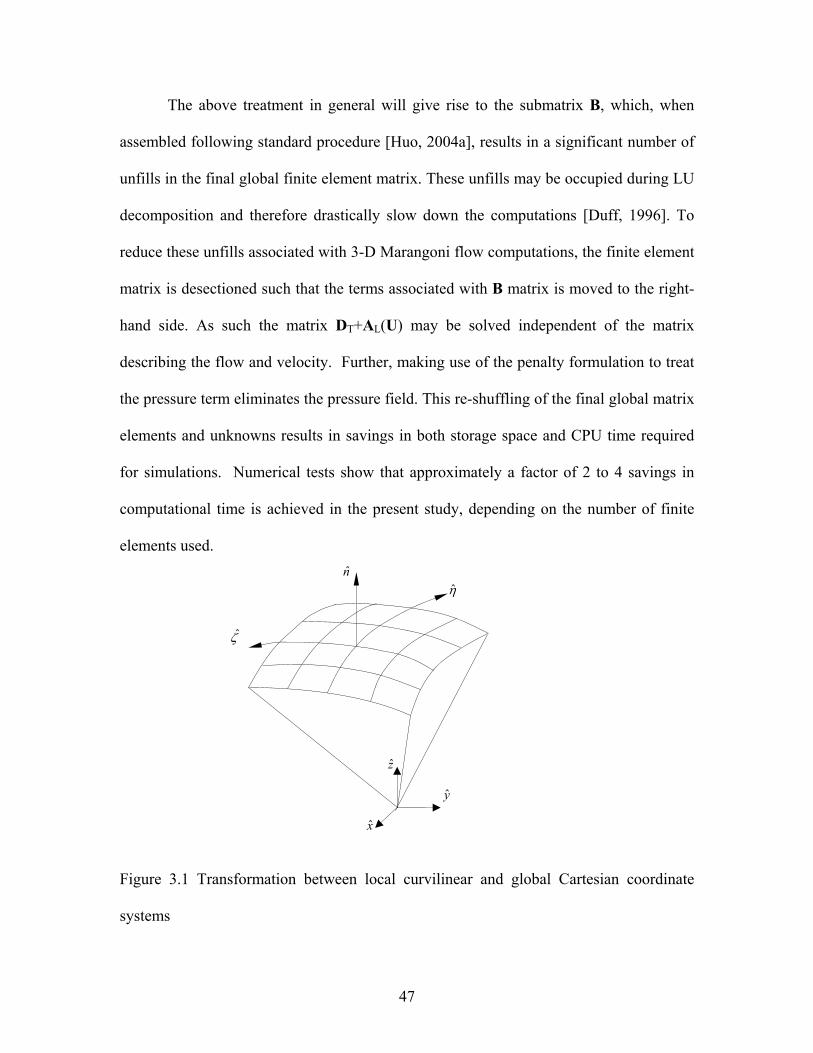
47

The above treatment in general will give rise to the submatrix B, which, when

assembled following standard procedure [Huo, 2004a], results in a significant number of

unfills in the final global finite element matrix. These unfills may be occupied during LU

decomposition and therefore drastically slow down the computations [Duff, 1996]. To

reduce these unfills associated with 3-D Marangoni flow computations, the finite element

matrix is desectioned such that the terms associated with B matrix is moved to the right-

hand side. As such the matrix DT+AL(U) may be solved independent of the matrix

describing the flow and velocity. Further, making use of the penalty formulation to treat

the pressure term eliminates the pressure field. This re-shuffling of the final global matrix

elements and unknowns results in savings in both storage space and CPU time required

for simulations. Numerical tests show that approximately a factor of 2 to 4 savings in

computational time is achieved in the present study, depending on the number of finite

elements used.

Figure 3.1 Transformation between local curvilinear and global Cartesian coordinate

systems

nη

ζ

x

y

z

48

3.4 Computation of the Stability of the Droplet in the Magnetic Fields

The 3-D electromagnetic field may be solved using the edge finite element method [Huo,

2004c, 2005b]. The edge-based elements are necessary to satisfy the divergence-free

constraint, ∇⋅E=0 [Johns, 1971]. However, the huge sparse matrix produced by the FEM

appears to be a major setback to finding an efficient numerical solution to a large scale

problem. Our experience shows that this remains true even with various efficient solvers

designed specifically for the solution of a large sparse system of linear algebraic

equations to improve the computational efficiency. To alleviate the disadvantage of the

finite element method, a hybrid finite element-boundary method is employed instead.

Using this approach, finite elements are used in the conducting droplet where power

density is needed and material properties may be a function of temperature, while

boundary elements are used elsewhere. The FEM and the BEM are coupled through the

interface boundary conditions. This idea is shown in Figure 3.2

Figure 3.2 Schematic representation of the coupling of the finite element and boundary

element

Ω1

Ω2

Interface of FEM and BEM

Ω1: FEM Ω2: BEM

49

3.4.1 Finite element formulation

To develop a finite element formulation in the conducting droplet, the wave equation

(2.51) is integrated with respect to a vector testing function δE [Akarapu, accepted].

dVjdV iV

crV

EJEEE δωµµεωµ

δ ⋅−=⎟⎟⎠

⎞⎜⎜⎝

⎛−×∇×∇⋅ ∫∫∫∫∫∫ 21 (3.43)

Integration by parts gives rise to the surface integral term,

( ) dVjdS

dVdV

iVS r

Vc

V r

JEnEE

EEEE

∫∫∫∫∫

∫∫∫∫∫∫

⋅−⋅×∇×

=⋅−×∇⋅×∇

ωµδδµ

δµεωδµ

1

1 2

(3.44)

Making use of the vector identity

( ) ( ) EEnnEE δδ ⋅×∇×−=⋅×∇× ˆˆ (3.45)

and also the boundary conditions, the final integral formulation is obtained,

50

[ ] dVjdS

dV

iVS

Vc

r

JEUE

EEEE

∫∫∫∫∫

∫∫∫⋅−⋅−

=⎟⎟⎠

⎞⎜⎜⎝

⎛⋅−×∇⋅×∇

ωµδδ

δµεωδµ

21

(3.46)

With appropriate finite element discretization and necessary elemental calculations

followed by assembly, one has the matrix representation of equation (3.46),

F[B]U[K]E =+ (3.47)

where the matrix elements are calculated using the following expressions,

dVKV

jicjir

ij ∫∫∫ ⎟⎟⎠

⎞⎜⎜⎝

⎛⋅−×∇⋅×∇= NNNN µεω

µ21

dSBS

jiij ∫∫ ⋅= SN

dVjFV

i ii JN ⋅−= ∫∫∫ ϖµ

Note that here Ni and Si are edge-based vector shape functions and their derivatives.

3.4.2 Boundary element formulation using the dyadic Green function

The basic idea of the hybrid FE/BE method was first introduced for the study of

electromagnetics by Silvester and Hsieh (1971) and McDonald and Wexler (1972) for

solving exterior or unbounded field problems. Later, the method was applied to solve

51

two- and three-dimensional antenna and scattering problems. Here, it is applied to solve

the electromagnetic field in a microwave system, and the formulation is based on Green’s

theorem involving the dyadic Green function,

( )( )( ) ( )( )dSGG

dSGG

dVGG

S

S

V

∫∫

∫∫

∫∫∫

⋅×∇×+×∇⋅×=

⋅×∇×−×∇×=

×∇×∇⋅−×∇×∇⋅

EnEn

nEE

EE

ˆˆ

ˆ (3.48)

Now, substituting into the above equation the following wave equations and the

equations for the dyadic Green function,

ijk JEE ωµ−=−×∇×∇ 20 (3.49)

( )'20 rr −=−×∇×∇ δIGkG (3.50)

and carrying out the necessary integration, we can get,

SdG

G

VdGZjkV

′′⋅′×∇′×′

+′×∇′⋅′×′

−′′⋅′−=

∫∫∫∫∫

)r(r,)]rE(n[

)]r(r,[)]rE(n[

)r(r,)r(JrE

S

0

0

000

ˆ

ˆ

)(

(3.51)

52

The surface’s unit normal direction points outward from the region Ω2. In equation

(3.51) the first term on the right-hand side is the field radiated by J in the free-space

environment, thus denoted as Einc. With the following relation,

IGG ×′∇′=×∇ )r(r,0' (3.52)

and the surface divergence theorem, equation(3.51) can be further simplified as

( ) ( ) ( )( )

( ) ( )( ) ( )'''ˆ''1

'ˆ'''ˆ

)()(

20

rrEnrr,

)(r'rr,)E(r'''nrr,)(r'En

rErE

dSGk

dSGG

S

S

inc

∫∫

∫∫

××∇⋅∇∇−

××∇+∇××

−=

(3.53)

Taking the cross product of equation (3.53) with surface normal n yields

( ) ( ) ( )( )

( ) ( )( ) ( )'''ˆ'',ˆ1

',''ˆ',''ˆˆ

ˆˆ

2 rrEnrrn

)(r'rr)(r'Enrr)(r'Enn

(r)En(r)En

dSGk

dSGG

S

S

inc

∫∫

∫∫

××∇⋅∇∇×−

××∇+∇×××

−×=×

(3.54)

After the BE discretization using edge boundary elements, followed by calculations at the

element level, equation (3.54) may be represented in the following matrix form,

53

tM

t

sttM

t

stssss U[][QE][PbE][Btt

∑∑ −−= (3.55)

where the matrix elements are calculated by

[ ] ( )∫∫ ⋅−=sS

Tss dS rSNBss

( )∫∫ ⋅=sS inc

s dS r(r)ESbs

[ ] ( ) ( ) ( )rrrrSSPst dSdSGs tS S

Tts∫∫ ∫∫ ∇×⋅= '','

[ ] ( ) ( ) ( )rrrrSSQst dSdSGs tS S

Tts∫∫ ∫∫⋅= '',

( ) ( ) ( )rrrrSS dSdSGks tS S

Tts∫∫ ∫∫ ⋅∇⋅∇− − '','2

With some matrix algebra, equation (3.55) is written more conveniently in the following

form,

22222 E]K[FU]B[ += (3.56)

where B2 is the boundary element matrix associated with the unknowns.

3.4.3 Coupling of boundary and finite elements

54

The boundary and finite element formulations for the solution of electric field distribution

are coupled through the interface conditions along the boundary of Ω1 and the boundary

of Ω 2,

22

11

ˆ1ˆ1 EnEn ×∇×=×∇×rr µµ

(3.57)

21 ˆˆ EnEn ×=× (3.58)

There are two ways to obtain a coupled solution of equations (3.47) and (3.56) with the

use of the above interface conditions. One way is to use direct coupling, by which the

entire boundary element region is treated as a macro element, and the boundary element

global matrix is then incorporated into equation (3.47). This approach works efficiently

for 2-D and moderately sized 3-D problems [Li, in print]. However, it becomes

inefficient for large 3-D problems such as the one under consideration because it

substantially increases the resultant edge finite element matrix bandwidth and hence the

CPU times. Another approach is iterative [Huo, 2004c, 2005b]. By this approach,

equation (3.56) is solved for U2 with an assumed E2 on the interface. The standard

LU-decomposition for complex matrix can be used for the solution. Then E1 is solved

using equation (3.47) with known U2. The convergence on |E2-E1|<ε, where ε is

the convergence criterion, is checked. If convergence is not achieved, E2=E1 along

the interface is used to predict an updated U2 using equation (19) and then E1 is

updated using equation (3.47). The process is repeated until the convergence is achieved.

55

It is worth noting here that for either of the two approaches, the matrix B2 requires

an LU-decomposition only once and the decomposed matrices are stored in the memory

for subsequent back substitutions when needed. In the case of the iterative procedure, this

means that subsequent iteration between FE and BE requires only a back substitution

procedure, thereby leading to a significant increase in computational speed.

3.5 Computation of the Oscillation of the Droplets in the Electrostatic Levitation

Mechanism

For the oscillation calculations, the electric and droplet deformation calculations must be

coupled with the fluid calculations. To incorporate the free surface boundary condition,

the front track technique is applied. Thus applying the weighted residuals method to Eq.

(2.37) results in the following matrix equations for the free surface boundary coordinates,

0KXXM =+& (3.59)

Because the nodes are allowed to move, these movements must be superimposed on the

velocity at the nodal points and therefore the convection term in Eq. (2.3) must be

modified accordingly, that is, uu ∇⋅ρ is replaced by uuv ∇⋅+ )(ρ where v is the nodal

velocity due to the free surface movement.

The oscillation calculations are solved iteratively with the time differentials

approximated by the implicit time differencing scheme. The iteration for the problem

starts the computation of the electric potential with an initial guess for the free surface,

56

then calculates fluid flow field, and then calculates the updated free surface boundary.

The updated boundary is used to start another set of calculation for the updated vector

potential and iteration continues till all the variables converge within a preset tolerance.

57

CHAPTER 4

3-D SIMULATION OF THE FREE SURFACE DEFORMATION AND

THERMAL CONVECTION IN THE ELECTROSTATICALLY LEVITATED,

SINGLE-PHRASE DROPLET

4.1 Introduction

In this chapter, a numerical study of steady state and transient 3-D Marangoni convection

and heat transfer in electrostatically levitated droplets. The analysis is based on the

Galerkin finite element solution of the Navier-Stokes and energy equations. Numerical

aspects for the computation of surface driven flows in general curvilinear coordinate

system are discussed within the framework of finite elements and differential geometry.

Results show that for practical microgravity conditions under which the deformation is

small, the single and double beam heating arrangements, when placed at the poles or

equator plane, produce an approximately axisymmetric flow profile and temperature

distribution with the axis of symmetry defined by the line passing through the centers of

the laser beam and the droplet. Thus, an axisymmetric model could provide a reasonably

good description, and an exact one when the laser beam is placed at a pole or one beam is

placed at both poles. When a tetrahedral or octahedral heating arrangement is applied,

complex 3-D flow structures occur, which result from interaction of flow motions

associated with each laser beam. For the case studied, the tetrahedral heating arrangement

does not seem to produce a significant reduction in internal velocity, in contrast to

perception, but the temperature is more uniform. This phenomenon is explained by the

58

fact that the 2-beam and 4-beam arrangements result in a surface temperature gradient of

approximately the same magnitude. The six-beam heating placement produces, however,

a much more significant reduction in both velocity and temperature non-uniformity. The

transient decaying during cooling is characterized by the evolution of both temperature

and velocity fields evolve in a rather complex fashion, with the initial stage dominated by

the pronounced thermal and flow mixing on the surface layer of a droplet. The strong

surface mixing quickly brings out a surface temperature distribution of axisymmetry,

while a 3-D structure still prevails inside until much later. The flow reversal is also

observed in the droplets that have been heated by 4- or 6-beam lasers during the decay,

and there is a spike in velocity and temperature at the time when the flow reversal occurs.

4.2 Result and discussion

The computational models described in chapter 3 may be employed to predict the electric

field distribution, electric pressure distribution along the surface of a droplet, droplet

shapes, transient full-3D temperature distribution and internal convection in the droplets

driven by surface tension force. Extensive numerical simulations have been carried out

for various heating conditions. A selection of computed results is given below. The

thermophysical properties used for calculations are tabulated in Table 4.1. The criterion

for the convergence of nonlinear iteration is set to 4101 −× (norm-2 relative error).

59

Parameters Values Tmelt (K) 1940

Q0 (W/m2) 1.3×106 ad (mm) 2.5

ρ (kg/m3) 4110 µ (kg/m-s) 5.2 x10-3

γ (N/m) 0.864 dγ/dT(N/m-K) -2.6 x10-4 Κ (W/m-K) 21.6 CP (J/kg-K) 700

E (V/m) 3.3 x106 Emisivity ε0 0.3

β (K-1) 6.5 x10-6 Pr 1.685 x10-1

al (mm) 2.05

Table 4.1 Parameters used in calculations of the thermal and fluid flow

4.2.1 Mesh selection and mesh independency test

Numerical tests show a total of 48 linear boundary elements were adequate for the

electric field calculations and 24 quadratic boundary elements for the computation of free

surface deformations. The thermal and fluid flow calculations used 8-node hexahedral

elements. Special treatment is made to generate the hexahedral elements neat the pole.

Mesh independence tests for flow and thermal simulations were conducted such that the

numerical error in two consecutive mesh refinements is smaller than 0.1% in maximum

velocities calculated. From these tests, a mesh of 2900 8-node elements was used for an

octant model for the results presented below, which is used to simulate 2 laser beams and

four laser beams, while that of 3680 8-node elements for a one-third model, to take

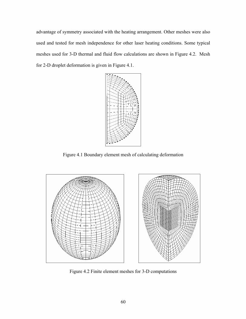
60

advantage of symmetry associated with the heating arrangement. Other meshes were also

used and tested for mesh independence for other laser heating conditions. Some typical

meshes used for 3-D thermal and fluid flow calculations are shown in Figure 4.2. Mesh

for 2-D droplet deformation is given in Figure 4.1.

Figure 4.1 Boundary element mesh of calculating deformation

Figure 4.2 Finite element meshes for 3-D computations

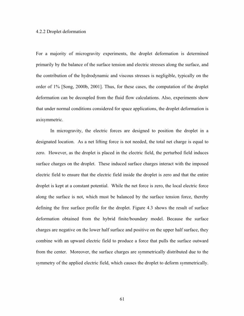
61

4.2.2 Droplet deformation

For a majority of microgravity experiments, the droplet deformation is determined

primarily by the balance of the surface tension and electric stresses along the surface, and

the contribution of the hydrodynamic and viscous stresses is negligible, typically on the

order of 1% [Song, 2000b, 2001]. Thus, for these cases, the computation of the droplet

deformation can be decoupled from the fluid flow calculations. Also, experiments show

that under normal conditions considered for space applications, the droplet deformation is

axisymmetric.

In microgravity, the electric forces are designed to position the droplet in a

designated location. As a net lifting force is not needed, the total net charge is equal to

zero. However, as the droplet is placed in the electric field, the perturbed field induces

surface charges on the droplet. These induced surface charges interact with the imposed

electric field to ensure that the electric field inside the droplet is zero and that the entire

droplet is kept at a constant potential. While the net force is zero, the local electric force

along the surface is not, which must be balanced by the surface tension force, thereby

defining the free surface profile for the droplet. Figure 4.3 shows the result of surface

deformation obtained from the hybrid finite/boundary model. Because the surface

charges are negative on the lower half surface and positive on the upper half surface, they

combine with an upward electric field to produce a force that pulls the surface outward

from the center. Moreover, the surface charges are symmetrically distributed due to the

symmetry of the applied electric field, which causes the droplet to deform symmetrically.

62

To satisfy the mass conservation, the droplet is squeezed at the equator, resulting in the

shape as shown.

It is noteworthy that an electrostatic field in general produces a potential apex that

is intrinsically unstable for the purpose of levitation. As a result, delicate dynamic control

system is required to make the levitation operation feasible. This is in contrast with

induction principle, which produces a potential wall for intrinsically stable

electromagnetic levitation.

-0.002 -0.001 0 0.001 0.002 0.003X (m)

-0.002

-0.001

0

0.001

0.002

0.003

Y(m

)

1

2

Figure 4.3 Comparison of free surface profiles of an electrically conducting droplet in

normal and microgravity: (1) E0=3.3 x 106 V/m and Q=0 C, and (2) un-deformed liquid

sphere.

63

4.2.3 Steady state fluid flow and temperature distribution

As stated before, the only non-zero Maxwell stress component on an electrically

conducting droplet is normal to the droplet surface in the natural coordinate, which

contributes to droplet deformation only. Therefore, the fluid flow in the droplet is caused

by the surface tension variation along the surface only, which in turn stems from a non-

uniform temperature distribution created by laser heating. While any types of heating

arrangements can be simulated with the numerical model described above, we consider

below four different types that are either used in practice or being considered for use in

the near future. These heating arrangements give rise to a complex 3-D flow structure,

except an axisymmetric placement of heating lasers.

(a) One laser beam on a pole or equator

Early practice of heating the sample in an electrostatic levitator is to apply one laser beam

at either the equator or one of the poles. When the laser beam is directed at the pole, the

flow field and temperature distribution are axisymmetric and thus a 2-D model is

sufficient to describe the transport phenomena. This 2-D model was reported in early

studies [Song, 2000b, 2001] and here it serves as a check on the 3-D model. The 3-D

model uses a quarter model consisting of a slice cut by two planes intersecting long the z-

axis. The comparison of the previous 2-D model and the present 3-D model results

indicates that the two produce the same flow pattern and agree within 0.1% (relative

error) in maximum velocities calculated, verifying that the 3-D model indeed reproduces

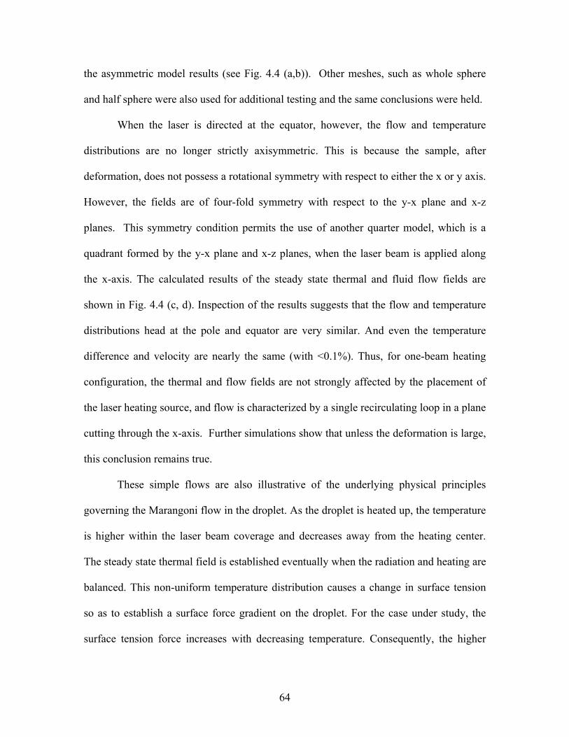
64

the asymmetric model results (see Fig. 4.4 (a,b)). Other meshes, such as whole sphere

and half sphere were also used for additional testing and the same conclusions were held.

When the laser is directed at the equator, however, the flow and temperature

distributions are no longer strictly axisymmetric. This is because the sample, after

deformation, does not possess a rotational symmetry with respect to either the x or y axis.

However, the fields are of four-fold symmetry with respect to the y-x plane and x-z

planes. This symmetry condition permits the use of another quarter model, which is a

quadrant formed by the y-x plane and x-z planes, when the laser beam is applied along

the x-axis. The calculated results of the steady state thermal and fluid flow fields are

shown in Fig. 4.4 (c, d). Inspection of the results suggests that the flow and temperature

distributions head at the pole and equator are very similar. And even the temperature

difference and velocity are nearly the same (with <0.1%). Thus, for one-beam heating

configuration, the thermal and flow fields are not strongly affected by the placement of

the laser heating source, and flow is characterized by a single recirculating loop in a plane

cutting through the x-axis. Further simulations show that unless the deformation is large,

this conclusion remains true.

These simple flows are also illustrative of the underlying physical principles

governing the Marangoni flow in the droplet. As the droplet is heated up, the temperature

is higher within the laser beam coverage and decreases away from the heating center.

The steady state thermal field is established eventually when the radiation and heating are

balanced. This non-uniform temperature distribution causes a change in surface tension

so as to establish a surface force gradient on the droplet. For the case under study, the

surface tension force increases with decreasing temperature. Consequently, the higher

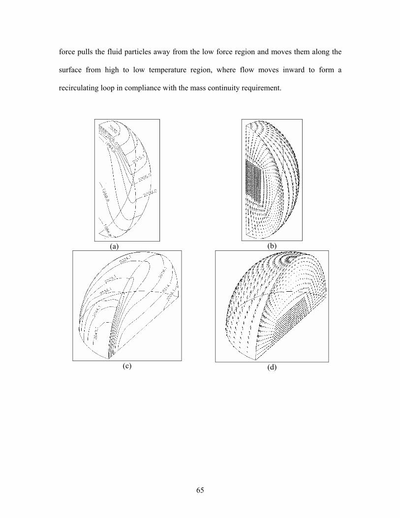
65

force pulls the fluid particles away from the low force region and moves them along the

surface from high to low temperature region, where flow moves inward to form a

recirculating loop in compliance with the mass continuity requirement.

(a)

(b)

(c)

(d)

66


deformed droplet under mcirogravity with a single beam heating laser: (a)-(b) for single

beam placed at the north pole -- Umax=14.64 (cm/s) and (c)-(d) for single beam placed at

the equator – Umax=14.43 (cm/s). Heat flux Q0=2.6×106 (W/m2).

(b) Two laser beams on the poles or equator

The use of two laser beams to heat the sample is also practiced. The two possible laser

beam arrangements are such that the beams are either applied at the two poles, which

give rise to a symmetric field distribution, or at the two opposite side of the equator. For

the former, a 2-D model is adequate [Song, 2000b], and thus provides once again a

checkpoint against which the 3-D model is tested. Computed results confirm that the 2-D

and 3-D model predictions are indeed in perfect agreement when the laser beams are

applied at the two poles. A 3-D view of the thermal and flow fields is presented in Fig.

4.5 (a, b). The two dimensional, axisymmetric flow structure is well predicted by the 3-D

model, as is expected. The temperature is higher at the poles and decreases towards the

equator. This establishes a surface force gradient by which the fluid particles are pulled

towards the equator at low temperature from the two poles that are at higher

temperatures. This, combined with the requirement of mass conservation, generates the

double toroidal recirculating flow loops.

To compare, two laser beams are applied symmetrically on the equator. The

radius of the laser beams is the same in the two cases. Strictly speaking, surface

67

deformation precludes the use of the rotational symmetry condition; but the 8-fold

symmetry is still applicable. As a result, only an octant is required for the calculations.

The computed results, showing the temperature and fluid flow distributions both on the

surface of and inside the droplet, are presented in Fig. 4.5 (c-f).

Comparison of the results in Fig. 4.5 reveals that the flow structures and

temperature distributions are similar for both cases. Detailed analyses, however, uncovers

that the rotational flow loop is only approximately symmetric around the axis formed by

connecting two heating sources applied at the equator, which is consistent with the

geometric constraint. Further numerical simulations show that a rotational symmetric

flow field is obtained if a droplet of perfect sphericity is heated with the two heating

sources placed at the two opposite sides of the equator. From Fig. 4.5, it is seen also that

the internal convection has a strong effect on the temperature distribution, which is

suggested by the distorted isothermal contour lines. For these two cases, the temperature

difference is 28.8 and the maximum velocity is 10.978 in the case of pole heating, which

compares 37.4 and 11.592, respectively, for the equator heating. Further simulations

show that with the same Qo and same radius of laser beams applied at the equator, the

average temperature is about 20K higher than heating at the poles, but the temperature

difference and hence the maximum velocity is roughly the same as those in Figs. 4.5 (a,

b).

68

(a) (b)

(c) (d)

(e) (f)


deformed droplet under mcirogravity with heating by dual lasers: (a) and (b) for beams

69

placed at north pole -- Umax=10.98 (cm/s) and (c)-(f) for beams placed at the equator –

Umax= 11.59 (cm./s). Heat flux Q= 1.3×106 (W/m2).

(c) Tetrahedral heating by four laser beams

Recently, there have been strong advocates in the droplet levitation community for the

use of a tetrahedral laser beam heating arrangement as a potential means to reduce the

temperature gradient in the droplet, thereby reducing the internal convection. In this

arrangement, four parts of the droplet surface are heated by lasers beams that are emitted

from the four corners of a tetrahedron whose geometric center is coincident with that of

the droplet. This design concept may be explored using the 3-D model before expensive

instrumentation is put in place, which in essence is the usefulness of a numerical model.

Because of the tetrahedral arrangement, symmetry conditions can be applied on the plane

that cuts through the two poles and the center of a laser beam placed around the droplet.

Thus a 1/3 model is sufficient to represent the complex flow and temperature field in the

droplet. The model used 3600 8-node finite element elements.

The calculated results are depicted in Figure 4.6. Clearly, tetrahedral heating

creates a rather complex flow structure, with fluid moving from four high temperature

regions to the low temperature regions (see Fig. 4.6 (a, c)). The complexity of fluid

motion is further revealed by the internal flows shown in Fig. 4.6(b, d). The four hot

spots are apparently associated with the laser heating and flows emerge from these hot

spots to find their ways to the regions where temperatures are low, as a result of surface

forces increasing with a decrease in temperature. Again, the internal flow recirculation

70

produce a strong effect on the temperature distribution, as is evident in the isothermal

contour plots viewed in slice cuts (Figs. 4.6 (a) and (c)).

Comparison of Figs. 4.5 and 4.6 exhibits that a tetrahedral heating arrangement,

though produces a more complex internal flow field, indeed gives much more uniform

temperature distribution inside the droplet: a temperature difference of 22.9 for

tetrahedral heating vs. that of 28.8 for dual laser heating. In sharp contrast with the

common perception, the maximum velocity generated by the tetrahedral heating is not

reduced significantly in accordance with the temperature reduction. In fact, only a small

reduction of velocity (11 %) is observed. This result, which is contradictory to what is

anticipated by four-beam advocates, may be explained as follows. While the temperature

difference indeed is much smaller with four laser beams than with two beams, the

temperature gradient along the surface is not as much different between the two cases,

thereby resulting in a reduction of velocity only by 11%. For example, detailed analyses

show that for the two beam cases, the temperature gradient between the hottest and

coldest spots on the surface is 7.334×103, which compares with 7.143×103 for four beam

lasers.

For surface tension driven flows, Marangoni number is often used as an indicator

of flow intensity. For electrostatically levitated droplets under consideration, however,

one can not use the Marangoni number based on a single characteristic length (say,

radius) to interpret the flows resulting from different heating arrangements for levitated

droplets, though it is legitimate for the same heating configuration. This is because the

length scales are different for different heating configurations, as discussed in the

71

paragraph above. A correct use of Marangoni numbers to characterize the flows must

take into the consideration the length scale changes for different heating arrangements.

(a) (b)

(c)

(d)


droplet under microgravity with tetrahedral heating arrangement: Umax=9.728 (cm/s).

Q= 0.65×106 (W/m2).

72

(d). Heating by six laser beams

Besides the dual and tetrahedral laser beam arrangements, other heating placements can

also be investigated using the numerical model described above. One of the viable

arrangements would be to use a 6-beam laser heating arrangement, symmetrically placed

with respect to the center of the droplet, for the purpose of further reducing the

temperature non-uniformity and a hope for a smaller flow velocity. One possible

arrangement is to slip the laser heating source into six laser beams, which will allow

heating to be applied equally on octahedrons of a droplet.

One such calculation is given in Fig. 4.7, where the 6 laser beams are arranged

such that two are at the poles and 4 beams are placed around the equator plane with equal

spacing, which are distributed at the 8 corners on the octahedron. Compared with the two

laser beams’ case, the calculated results indicate that the temperature gradient is reduced

about 50% and so is the internal velocity with this arrangement. A detailed inspection of

these flow structures, although very complex, seems to suggest that these complex flow

structures are a result of interaction of the Marangoni flow cells associated with each

laser beams.

A summary of major results calculated for different heating arrangements is given

in Table 4.2.

73

(a) (b)

(c)

(d)


droplet under microgravity with octahedral heating arrangement: Umax=5.321 (cm/s).

Q= 1.3×106/3 (W/m2).

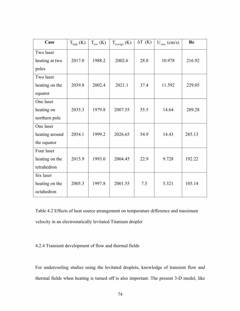
74

Case (K) Thigh (K) Tlow (K) Taverage (K) T∆ (cm/s) Umax Re

Two laser

heating at two

poles

2017.0

1988.2

2002.6

28.8

10.978

216.92

Two laser

heating on the

equator

2039.8

2002.4

2021.1

37.4

11.592

229.05

One laser

heating on

northern pole

2035.3

1979.8

2007.55

55.5

14.64

289.28

One laser

heating around

the equator

2054.1

1999.2

2026.65

54.9

14.43

285.13

Four laser

heating on the

tetrahedron

2015.9

1993.0

2004.45

22.9

9.728

192.22

Six laser

heating on the

octahedron

2005.3

1997.8

2001.55

7.5

5.321

105.14

Table 4.2 Effects of heat source arrangement on temperature difference and maximum

velocity in an electrostatically levitated Titanium droplet

4.2.4 Transient development of flow and thermal fields

For undercooling studies using the levitated droplets, knowledge of transient flow and

thermal fields when heating is turned off is also important. The present 3-D model, like

75

its 2-D counterpart [Song, 2001b], is also capable of describing the transient development

of both 3-D fluid flow and temperature distribution in an electrostatically levitated

droplet. Figs. 4.8 and 4.9 show the time development of 3-D fluid flow and thermal fields

in droplets heated by 4-beam and 6-beam arrangements, respectively. Apparently, the

transient fluid flow structure evolves in time differently for the two cases. The transient

simulations of axisymmetric thermal and fluid flow fields induced by single and double

beams were discussed in a previous paper on 2-D models.

Inspection of Figs. 4.6 and 4.8 shows that in the case of the 4-laser beam

arrangement, the temperature field changes very rapidly when the heating is turned off,

which causes a flow reversal near the north pole region and a change in flow structure in

the droplet. At time t=0.28 seconds after the laser beams are switched off, the surface

temperature is largely smeared out due to both convection and radiation such that the

temperatures at the north pole is reduced below everywhere, a manifestation of high heat

lose there. In three other heating regions, however, the temperature remains relatively

higher. This is explained by the fact that for the same laser beam diameter, the surface

areas form which heat loss occurs are much smaller because of a much larger surface

curvature radius in these regions. Note also that there exists considerable thermal mixing

along the azimuthal direction, which brings the temperature into an axisymmetric field.

The consequence of this change in thermal fields is that one smaller toroidal loop near the

north pool is engulfed by the loop associated with the side heating source. This

phenomenon is consistent with the underlying physics governing the surface tension

driven flows discussed in the above section (c).

76

Turning to the time evolution of the thermal and fluid flow fields induced by the

6-beam heating arrangement, one can see that the similar phenomena are observed in that

a lower temperature occurs in the pole regions and the temperature is smeared

considerably along the azimuthal direction. This is accompanied by the flow change such

that the complex flow structure characterized by several recirculating regions is now

replaced by basically two large toroidal flow loops recirculating above and below the

equatorial plane, as shown in Fig. 4.9.

To further assess the dynamics of the transient thermal and flow fields,

information on the history of velocity and temperature at some specific locations is

obtained. Fig. 4.10 shows the decay of maximum velocities and the maximum and

minimum temperature differences in the droplet heated by 4- and 6-beams after heating

sources are turned off. It is seen that during the first 0.5 seconds after lasers are shut off,

both velocities and temperature differences experience dramatic change and then decay

gradually afterwards. After an elapse of 3 seconds, the maximum velocities reach

essentially the same level in the droplet heated initially by either 4- or 6-beams. The

maximum velocity changes in accordance with the temperature differences, in

compliance with the basic principle of surface tension driven flows. Examination of these

transient results along with 3-D views of flow visualization illustrates that the time at

which the velocity and temperature spikes up (t~0.3 sec) corresponds to the time when

the internal flow starts to reverse its flow pattern in certain regions, as shown in Figs. 4.8

and 4.9.

Although the temperature differences undergo drastic changes, the temperatures at

specific locations do not necessarily do so. Typical time change in temperature and

77

velocity at specific locations are compared in Fig. 4.11 for the droplets heated by 4- and

6-beams. Compared with Fig. 4.10, these results show that the temperature at the specific

point decays more smoothly, although the maximum and minimum temperature

differences vary more drastically during the initial transient period. The temperature at

this point decreases by about 260K below the steady temperature or 200 K below the

melting temperature. The velocity at the point where the highest steady-state temperature

is attained decays very quickly initially and remains approximately constant afterwards.

The evolution of temperature distributions along a line emitting from the center to

a point on the droplet surface is plotted in Figs. 4.12 (a) and (b) for 4-beam and 6-beam

heating arrangements, respectively. These results show that the steady state temperature

distribution is rather uniform and as temperature drops, the temperature distribution

changes more rapidly. The largest change occurs at around t~0.25 seconds. Note that for

clarity of the plots, different scales are used for the temperature distribution at t=3

seconds, at which time a temperature difference between the center and the surface is

~7K is obtained for the 4-beam case and ~5K for the 6-beam case.

78

(a) (b) Temperature and flow at 0.07 second

(c) (d) Temperature and flow at 0.28 second

Figure 4.8 Snapshots of thermal and melt flow fields during their decay as heating lasers

are turned off: (a) temperature distribution and (b) velocity field (Umax=4.376 (cm/s)) at

t=0.07 sec., and (c) thermal field and (d) velocity profile (Umax=6.941 (cm/s)) at t=0.28

sec. The initial conditions for the calculations are given in Fig. 4.6.

79

(a) (b) Temperature and flow at 0.04 second

(c) (d) Temperature and flow at 0.22 second

Figure 4.9 Snapshots of thermal and melt flow fields during their decay as heating lasers

are turned off: (a) temperature distribution and (b) velocity field (Umax=3.812 (cm/s)) at

t=0.04 sec., and (c) thermal field and (d) velocity profile (Umax =6.561 (cm/s)) at t=0.22

sec. The initial conditions for the calculations are given in Fig. 4.7.

80

0

0.02

0.04

0.06

0.08

0.1

0.12

0 0.5 1 1.5 2 2.5 3Time (second)

Max

imum

Vel

ocity

(m/s

)

0

5

10

15

20

25

Tem

pera

ture

diff

eren

ce (k

)

Figure 4.10 Decaying history of maximum velocities and the maximum and minimum

temperature differences in the droplets heated by 4-beam and 6-beam heating lasers, after

heating is switched off.

1. ∆T (6 beams)2. ∆T (4 beams)

3. Vmax (6 beams) 4. Vmax (4 beams)

81

0

0.02

0.04

0.06

0.08

0.1

0.12

0 0.5 1 1.5 2 2.5 3Time (second)

Velo

city

(m/s

)

1700

1750

1800

1850

1900

1950

2000

2050

Tem

pera

ture

(K)

Figure 4.11 Transient development of velocities and temperatures at specific points in the

droplets heated by 4-beam and 6-beam heating lasers, after heating is switched off. The

velocities are monitored at (x= 4103106.9 −× ,y= 4103755.5 −× ,z= 3105955.2 −×− all in

meters) for 4-beam and at ( 4109974.2 −×− , 3108925.1 −× , 3106365.1 −× ) for 6-beam

where the maximum steady state velocities are attained. The temperatures are monitored

at ( 3108425.1 −× , 3100638.1 −× , 3101372.1 −×− for 4-beam and at ( 0,103075.2,0 3−× ) for

6-beam where the maximum steady state temperatures occur in the droplets.

1. Th (4 beams)

2. Th (6 beams)

3. V (4 beams)4. V (6 beams)

82

1965

1970

1975

1980

1985

1990

1995

2000

2005

2010

0 0.0005 0.001 0.0015 0.002 0.0025 0.003

Distance (m)

Tem

pera

ture

(k)

1742

1743

1744

1745

1746

1747

1748

1749

1750

Tem

pera

ture

at 3

sec

ond

0.0 second0.07 second0.28 second3 second

(a)

1970

1975

1980

1985

1990

1995

2000

2005

0 0.0005 0.001 0.0015 0.002 0.0025 0.003

Distance (m)

Tem

pera

ture

(K)

1740

1741

1742

1743

1744

1745

1746

Tem

pera

ture

at 3

sec

ond

0 second0.04 second0.22 second3 second

(b)

Figure 4.12 Evolution of temperature distributions along the line emitted from the center

of the droplet to (0,1,1) on the surface for (a) tetrahedral and (b) octahedral heating

arrangements. The curve at t=3 seconds refers to the vertical axis at right.

83

4.3 Concluding Remarks

This chapter has presented a numerical model for steady-state and transient 3-D

Marangoni convection and heat transfer in electrostatically levitated droplets. The

numerical model development is based on the Galerkin finite element solution of the

Navier-Stokes and energy equations. Numerical aspects for the computation of surface

driven flows in general curvilinear coordinate system have been discussed within the

framework of finite elements and differential geometry. Results of droplet deformation

by electrostatic forces and both steady-state and transient 3-D Marangoni flows in

droplets heated by a variety of heating source arrangements have been presented. For

practical microgravity conditions under which the deformation is small, the single and

double beam heating arrangements, when placed at the poles (or equator plane), produce

exactly (or approximately) axisymmetric flow profile and temperature distribution with

the axis of symmetry defined by the line passing through the centers of the laser beam

and the droplet. As such a 2-D axisymmetric model could provide a reasonably good

description, and an exact one when placed at the poles. Complex 3-D flow structure

emerges when a tetrahedral or octahedral heating arrangement is applied. These complex

flow structures result from the interaction of melt flows associated with each laser beam.

For the case studied, the tetrahedral heating arrangement does not seem to produce a

significant reduction in internal velocity, in contrast to perception, while the temperature

is more uniform. This is attributed to the fact that the 2-beam and 4-beam arrangements

result in a surface temperature gradient of approximately the same magnitude. While the

Marangoni numbers are able to characterize the flow for a same heating arrangement, a

84

correct use of them needs to factor in the different length scales associated with different

heating placements. The six-beam heating placement produces, however, a much more

significant reduction in both velocity and temperature non-uniformity. During the

transient decaying, both temperature and velocity fields evolve in a complex fashion with

the initial stage dominated by the thermal and flow mixing on the surface of a droplet that

has been heated by 4- or 6-beam lasers. The flow reversal is also observed in the droplets

during the decay, and a spike in velocity and temperature is found at the time when the

flow reversal is taken place. The strong surface mixing quickly brings out a surface

temperature distribution of axisymmetry, while inside the droplet the 3-D structure still

persists until much later.

85

CHAPTER 5

3-D SIMULATION OF MASS TRANSFER IN THE ELECTROSTATICALLY

LEVITATED, SINGLE-PHRASE DROPLET

5.1 Introduction

In this chapter, a mathematical model is developed for the solute transport phenomena in

electrostatically levitated droplets under microgravity, based on the computational results

of the free surface deformation, full 3-D Marangoni convection in chapter 4. The thermal

transport in the droplet is conduction-dominant for the cases studied. In general, the

convection is stronger with higher melting point melts. The internal convection has a

strong effect on the concentration distribution in the droplet. For melts with high

viscosities, a significant reduction in velocity can be achieved with an appropriate laser

beam arrangement, thereby permitting a diffusion-controlled condition to be developed.

5.2 Results and Discussion

Solute distribution in electrostatically positioned droplets is calculated using the

numerical procedure as described in chapter 3. Numerical simulations were carried out

and a selection of computed results is presented below. The physical properties used for

calculations are listed in Table 5.1. The mesh independence testing procedure for droplet

deformation and internal convection computations has been discussed in the chapter 4.

Because of the small magnitude of mass diffusion coefficient (D) (See Table 5.3), a

86

denser mesh is needed to obtain mesh independent results. Therefore, the simulation of

mass transfer used 8,036 8-node elements for the two- and six-beam cases and 9,184 8-

node elements for the four-beam case, respectively. The velocity fields are interpolated

from the coarse mesh to the dense mesh. Numerical simulations were also made for

selected cases using the dense meshes to ensure no loss in accuracy due to interpolation.

The meshes used for shape deformation calculations and for the mass diffusion are

illustrated in Fig. 5.1. The mesh distribution for the thermal and flow calculations is

similar to chapter 4 and thus not shown. The convergent criterion of 1×10-4 (relative

error) is set for the nonlinear iteration of the droplet shape coordinates and the

temperature, velocity and concentration fields.

Let us turn our attention to the solute transport in the droplets. While the

mathematical model described here has no limitations of where and when to add the

solutal elements into the droplet, a special situation is considered here where a mass flux

method is used to deposit a solutal element on the molten droplet when the flow reaches a

quasi-steady state. The deposition rate is assumed such that the concentration on the

droplet surface is maintained as a constant. As a first approximation, the surface tension

is assumed to be the same as the pure material into which solutal elements are added.

This assumption is thought to be reasonable so long as the concentration is dilute, say 5

to 10% [Johnson, 2002]. This allows the calculation of solute transport to be decoupled

from the thermal and flow calculations. The effects of the mixture need to be considered

if the concentration is high, however; and when this happens, the concentration

distribution must be calculated together with the thermal and flow fields.

87

Figure 5.2 depicts a set of snap shots of concentration distributions in levitated

droplets heated by two-beam, four-beam and six-beam arrangements. As a comparison,

the concentration distribution under pure diffusion is also given in Figure 5.2 (g-h).

Comparison of these results illustrates the significant effect of the internal convection on

the concentration distribution in the liquid Al droplet. Clearly, for the droplet under

consideration, the mass transport is convection dominant. This is also supported by the

ratios of the diffusion velocity and the convection velocity is given in Table 5.3. It is

noted that in the case of the six-beam heating arrangement the flow is less intensive and

thus a longer time duration is selected to show the convection effects.

To further understand the mass transport phenomena in the droplet, the

concentration distribution along several different radial directions originating from the

center of the droplet to its surface is plotted at t = 0.5 second. The results are shown in

Figure 5.3. The effects of convection on the concentration distribution are evident,

confirming the conclusions drawn from the above 3-D contour distributions.

As discussed before, a more vigorous internal flow occurs in the droplets of

higher melting point and thus should have a stronger effect on solute distribution. From

Table 5.1, it is seen that there exists a much larger velocity in the molten Fe droplet,

which results in a more pronounced effects on solute transport. This is further confirmed

by the results given in Figure 5.4, where the Si and Ti concentrations at the center of the

droplet reaches a quasi-steady state in the Fe droplet much more quickly than the Cu and

Fe concentrations in the Al droplet. The 3-D view of the Si and Ti concentration

contours, however, is similar to those given above.

88

One of the important applications of electrostatically levitated droplets is to

develop a diffusion-dominating condition in a larger sample for both fundamental

materials science studies and for physical property measurements, which would

otherwise be difficult to obtain on Earth. To achieve this, the Magangoni convection in

the droplet must be controlled below the diffusion velocity so that the concentration

profile is predominant by diffusion mechanism. The present mathematical model should

be useful to test the novel concepts developed along these lines. Many numerical

simulations were conducted with the model. It is found that a logical approach would

have to rely on an appropriate choice of materials and the heating source configurations.

One case study is given here, which is concerned with measuring diffusion

coefficients of Cu in a glass forming metal using an electrostatically-positioned droplet

under microgravity, which is described in [Johnson, 2002]. The parameters used for

calculations are given in the third column of Table 5.1. Computations follow the same

procedures as described above, that is, the droplet deformation calculation is followed by

the thermal and fluid flow and mass transfer calculations. While the flow patterns are

very similar to those described above, the flow intensity is drastically reduced because of

a much higher viscosity of this material (see Table 5.2). Figure 5.5 displays the

concentration distributions in this droplet being heated by three different heating

arrangements. The pure-diffusion-controlled concentration contour is also plotted as a

comparison. Examination of these results indicates that both two-beam and tetrahedral

beam arrangements provide a distorted concentration profile, suggesting that for these

two heating arrangements the Marangoni convection is still significant and the mass

transfer is not diffusion-dominant. However, the six-beam arrangement gives a

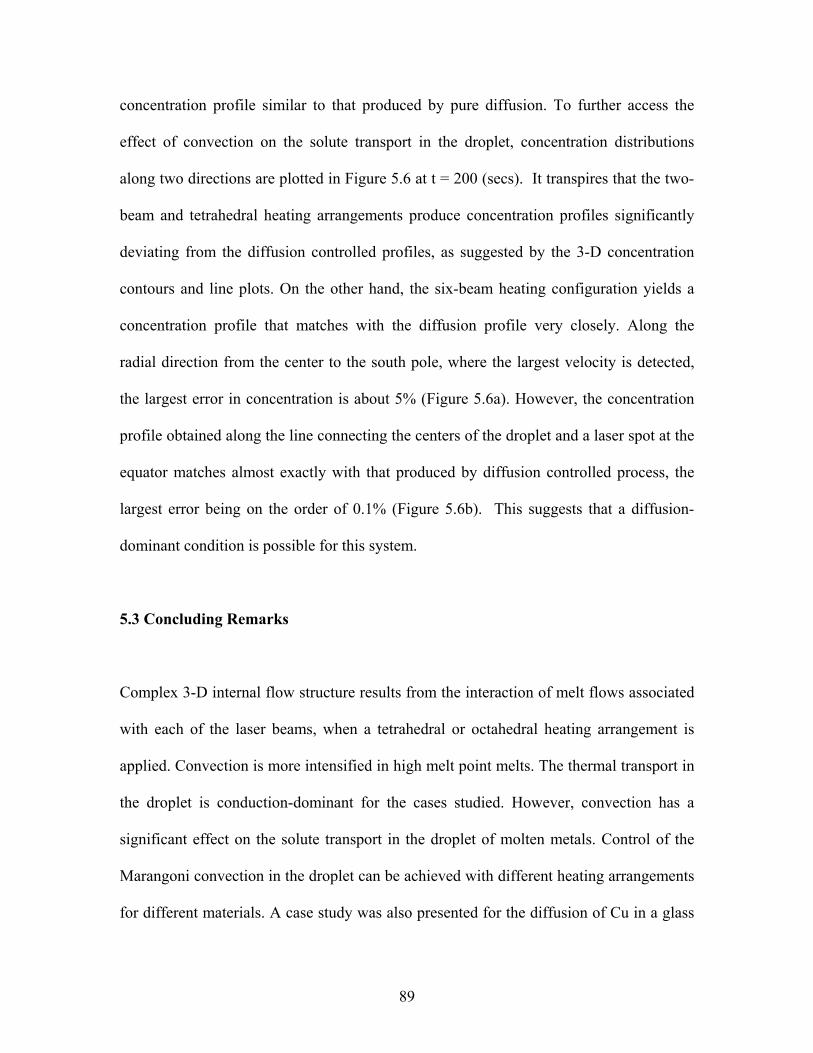
89

concentration profile similar to that produced by pure diffusion. To further access the

effect of convection on the solute transport in the droplet, concentration distributions

along two directions are plotted in Figure 5.6 at t = 200 (secs). It transpires that the two-

beam and tetrahedral heating arrangements produce concentration profiles significantly

deviating from the diffusion controlled profiles, as suggested by the 3-D concentration

contours and line plots. On the other hand, the six-beam heating configuration yields a

concentration profile that matches with the diffusion profile very closely. Along the

radial direction from the center to the south pole, where the largest velocity is detected,

the largest error in concentration is about 5% (Figure 5.6a). However, the concentration

profile obtained along the line connecting the centers of the droplet and a laser spot at the

equator matches almost exactly with that produced by diffusion controlled process, the

largest error being on the order of 0.1% (Figure 5.6b). This suggests that a diffusion-

dominant condition is possible for this system.


Complex 3-D internal flow structure results from the interaction of melt flows associated

with each of the laser beams, when a tetrahedral or octahedral heating arrangement is

applied. Convection is more intensified in high melt point melts. The thermal transport in

the droplet is conduction-dominant for the cases studied. However, convection has a

significant effect on the solute transport in the droplet of molten metals. Control of the

Marangoni convection in the droplet can be achieved with different heating arrangements

for different materials. A case study was also presented for the diffusion of Cu in a glass

90

forming metal alloy, which has a high viscosity. For this metal alloy, a significant

reduction in velocity can be achieved and the concentration distribution along some

directions matches well with the diffusion controlled profile, when a six laser-beam

arrangement is used.

Table 5.1 Parameters used for calculations

Parameters Al Fe Metallic glass forming liquid [4,21] Tmelt (K) 934 1809

Q0 (W/m2) 0.97×105 1.1×106 6.0×104 ad (mm) 2.5 2.5 5.0 al (mm) 2.0 2.0 7.0

ρ (kg/m3) 2385 7015 6000 (Est.) µ (kg/m-s) 1.3×10-3 5.5×10-3 5 (Est.)

γ (N/m) 0.914 1.872 1.2 (Est.) Dγ/dT(N/m-K) -3.5×10-4 -4.9×10-4 -3.0×10-4 (Est.)

Κ (W/m-K) 95.37 78.2 20 (Est.) CP (J/kg-K) 1080 795 50 (Est.)

E (V/m) 2.5×106 3.3×106 2.5×106

Emisivity ε0 0.3 0.3 0.3 Pr 1.472×10-2 5.591×10-2 12.5

Taver (K) 996 1918 1080

Table 5.2 Maximum velocity and temperature difference in droplets

Al Fe Metallic glass forming liquid Cases 2 4 6 2 4 6 2 4 6

Vmax (cm/s) 3.50 1.92 0.94 9.04 6.02 2.90 5.8×10-3 1.1×10-3 1.5×10-4

∆T (K) 1.28 0.57 0.21 12.19 6.90 2.23 8.7 1.6 0.2

Vmax, ∆T, and Re at different laser heatings Re 160 88 43 288 192 92.5 4.9×10-4 9.2×10-5 1.26×10-5

Table 5.3 Diffusion coefficients and Vmax/Vdiff for cases studied

Materials Al-Cu Al-Fe Fe-Si Fe-Ti Metallic glass forming liquids-liquid metal

Diffusion coefficient Do×105 (cm2/sec) 7.2 1.4 11 32 1 (Est.)

Diffusion velocity ×105 (m/s) 1.22 1.22 1.22 1.22 1.22

Vmax/Vdiff (for 2 laser beams) 2.87×103 2.87×103 7.40×103 7.40×103 4.75



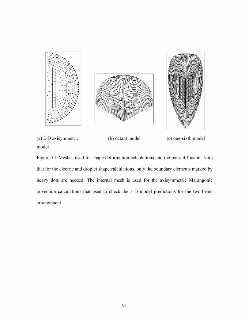
91

(a) 2-D axisymmetric

model

(b) octant model (c) one-sixth model

Figure 5.1 Meshes used for shape deformation calculations and the mass diffusion. Note

that for the electric and droplet shape calculations, only the boundary elements marked by

heavy dots are needed. The internal mesh is used for the axisymmetric Marangonic

onvection calculations that used to check the 3-D model predictions for the two-beam

arrangement

92

(a) t=0.1 sec

(b) t=0.3 sec

(c) t=0.2 sec

(d) t=0.4 sec

(e) t=0.6 sec

(f) t=0.8 sec

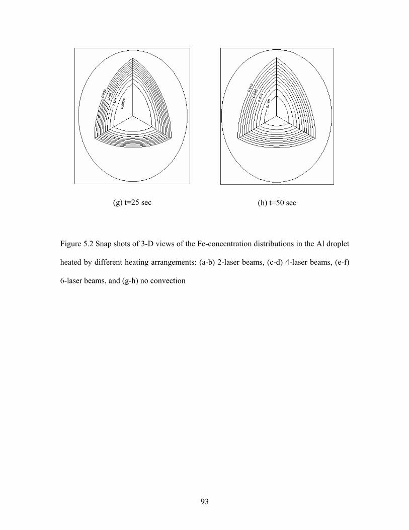
93

(g) t=25 sec

(h) t=50 sec

Figure 5.2 Snap shots of 3-D views of the Fe-concentration distributions in the Al droplet

heated by different heating arrangements: (a-b) 2-laser beams, (c-d) 4-laser beams, (e-f)

6-laser beams, and (g-h) no convection

94

0

0.1

0.2

0.3

0.4

0.5

0.6

0.7

0.8

0.9

1

0 0.2 0.4 0.6 0.8 1

Con

cent

ratio

nno convection2 laser beams4 laser beams6 laser beams

Figure 5.3 Concentration distribution along the line originating from the center (0, 0, 0)

to the surface of the Al droplet at t = 0.5 second. The line has an angle of 450 above the

equator plane (the unit vector of the line: 3213

13

13

1 iiir ++= ). The distance is non-

dimensionalized by the radius of the droplet. The convection-dominant concentration

profiles deviate drastically from the pure-diffusion profiles.

95

0

0.2

0.4

0.6

0.8

1

0 0.1 0.2 0.3 0.4 0.5Time (second)

Con

cent

ratio

n

Figure 5.4 Time evolution of the Si and Ti concentrations at the center of the Fe droplet

and the Cu and Fe concentrations at the center of the Al droplet. Strong flows in the Fe

droplet quickly brings the solute from the surface to the center. The concentration is non-

dimensionalized

12 4

3

1. Al-Fe 2. Al-Cu 3. Fe-Si 4. Fe-Ti

96

(a) no convection

(b) 2 laser beams

(c) 4 laser beams

(d) 6 laser beams

Figure 5.5 A 3-D view of concentration contours in the metallic glass forming droplet

heated by different heating arrangements (t = 200 seconds): (a) no convection, (b) 2-laser

beams, (c) 4-laser beams, and (d) 6 laser beams

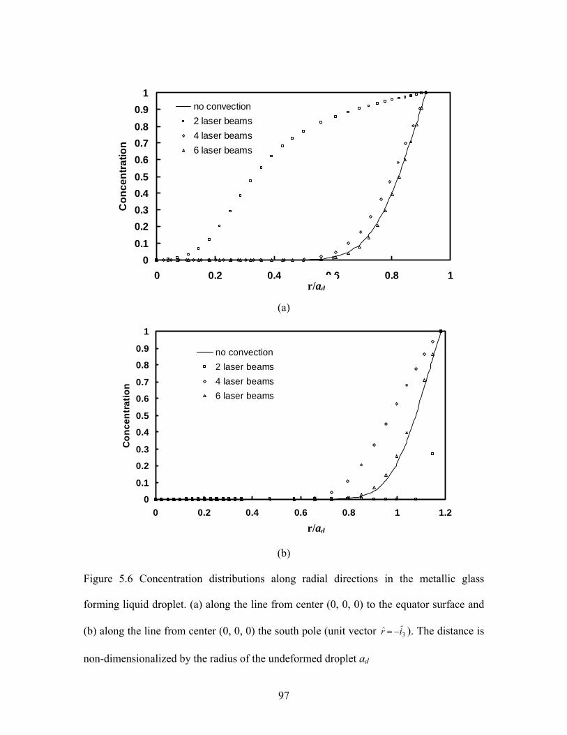
97

00.10.20.30.40.50.60.70.80.9

1

0 0.2 0.4 0.6 0.8 1

Con

cent

ratio

nno convection2 laser beams4 laser beams6 laser beams

(a)

0

0.1

0.2

0.3

0.4

0.5

0.6

0.7

0.8

0.9

1

0 0.2 0.4 0.6 0.8 1 1.2

Con

cent

ratio

n

no convection2 laser beams4 laser beams6 laser beams

(b)

Figure 5.6 Concentration distributions along radial directions in the metallic glass

forming liquid droplet. (a) along the line from center (0, 0, 0) to the equator surface and

(b) along the line from center (0, 0, 0) the south pole (unit vector 3ir −= ). The distance is

non-dimensionalized by the radius of the undeformed droplet ad

r/ad

r/ad

98

CHAPTER 6

2-D SIMULATION OF THE THERMAL CONVECTION IN THE

ELECTROSTATICALLY LEVITATED DROPLET OF IMMISCIBLE LIQUID

METALS

6.1 Introduction

In this chapter, a numerical study is presented of the free surface deformation and

Marangoni convection in immiscible droplets positioned by an electrostatic field and

heated by laser beams under microgravity. The boundary element and the weighted

residuals methods are applied to iteratively solving the electric field distribution and the

unknown free surface shapes. The Galerkin finite element method is employed to solve

the thermal and fluid flow field in both the transient and steady states. Results show that

the inner interface demarking the two immiscible fluids in an electrically conducting

droplet is immune to the applied electrostatic field and maintains its sphericity in

microgravity under steady state conditions. The free surface or, however, deforms into an

oval shape in an electric field and its equilibrium shape is determined by the balance of

the Maxwell stress and the surface tension. The deformation is attributed to the pulling

action of the normal component of the Maxwell stress. The thermal and fluid flow

distributions are rather complex in an immiscible droplet. The dominant mechanism for

the thermal transport in the droplet is by conduction and convection plays only a minor

role. The flow near the free surface is driven by the Marangoni forces, which cause the

fluid particles to move from high to low temperature regions. The flow in the inner core

99

and near the immiscible interface, however, is driven by a competing mechanism

between the thermally induced interfacial surface tension gradient and the inertia force in

the outer fluid layer. During cooling into an undercooled state after the laser heating is

switched off, surface radiation results in a reversal of the surface temperature gradients

both along the free surface and along the immiscible interface. This change in the thermal

gradients reverses the surface tension driven flow in the outer layer. The flow near the

interfacial region is complex and is driven by a complimentary mechanism between the

interfacial and the inertia forces during the time when the thermal gradient on the free

surface is reversed and that on the interface is not. Before and after the completion of the

interfacial thermal gradient reversal, however, the interfacial flows are determined by the

competing mechanism between the interfacial and inertia forces.


The computational model developed above enables the prediction of the electric field

distribution, the Maxwell stress distribution along the surface of a droplet, droplet shapes,

temperature distribution and internal convection within the droplets driven by surface

tension and buoyancy forces in normal gravity. A selection of computed results is

presented for some immiscible droplets being considered for microgravity applications.

Unless otherwise indicated, the computations used the physical properties and parameters

in Table 6.1. It is noted that Qc is the critical charge as predicted by Rayleigh’s theory

[Rayleigh, 1882], above which a charged drop becomes unstable and starts to break into

smaller droplets. A total of 48 linear boundary elements were used for the electric

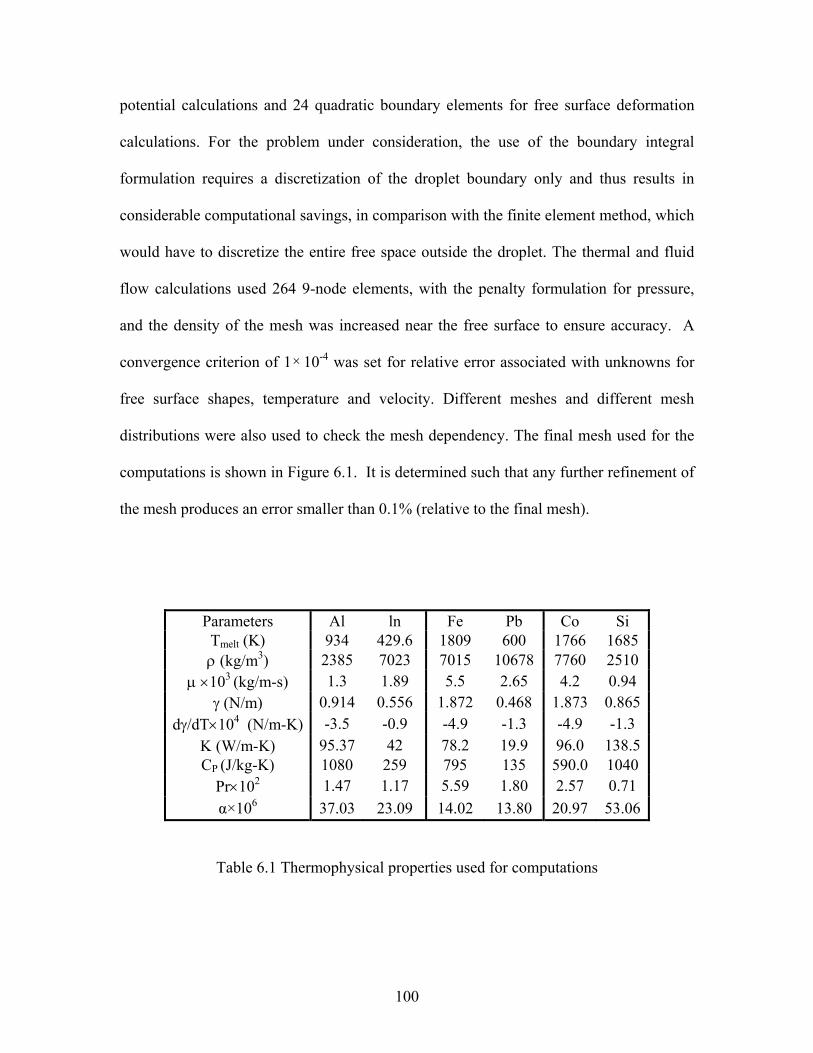
100

potential calculations and 24 quadratic boundary elements for free surface deformation

calculations. For the problem under consideration, the use of the boundary integral

formulation requires a discretization of the droplet boundary only and thus results in

considerable computational savings, in comparison with the finite element method, which

would have to discretize the entire free space outside the droplet. The thermal and fluid

flow calculations used 264 9-node elements, with the penalty formulation for pressure,

and the density of the mesh was increased near the free surface to ensure accuracy. A

convergence criterion of 1 × 10-4 was set for relative error associated with unknowns for

free surface shapes, temperature and velocity. Different meshes and different mesh

distributions were also used to check the mesh dependency. The final mesh used for the

computations is shown in Figure 6.1. It is determined such that any further refinement of

the mesh produces an error smaller than 0.1% (relative to the final mesh).

Parameters Al ln Fe Pb Co Si Tmelt (K) 934 429.6 1809 600 1766 1685 ρ (kg/m3) 2385 7023 7015 10678 7760 2510

µ ×103 (kg/m-s) 1.3 1.89 5.5 2.65 4.2 0.94 γ (N/m) 0.914 0.556 1.872 0.468 1.873 0.865

dγ/dT×104 (N/m-K) -3.5 -0.9 -4.9 -1.3 -4.9 -1.3 Κ (W/m-K) 95.37 42 78.2 19.9 96.0 138.5 CP (J/kg-K) 1080 259 795 135 590.0 1040

Pr×102 1.47 1.17 5.59 1.80 2.57 0.71 α×106 37.03 23.09 14.02 13.80 20.97 53.06

Table 6.1 Thermophysical properties used for computations

101

Figure 6.1 Boundary element and finite element mesh for numerical computation

6.2.1 Droplet deformation

There are two interfaces associated with an immiscible droplet. The outer surface is a free

surface that separates the droplet from free space. The inner surface is an interface that

demarks the two immiscible fluids. Analyses are made to understand the reaction of

these interfaces to an imposed electric field, which is used to position the droplet under

microgravity.

We first consider the behavior of the inner interface. It is known that when an

electric conductor is placed in an electric field, electric charges are induced on its surface.

These charges induce an electric field inside the droplet just opposite to the applied field

so that the total inside field is identically zero. This is the renowned Gaussian law of

electrostatics, which requires that the whole droplet be at the equal potential and the

surface charges appear only on the free (or outer) surface of the droplet. This means that

102

the Maxwell stress along the immiscible interface is zero and the inner interface shape is

completely determined by the balance of the hydrodynamic forces along the interface

face, or the balance of the surface effect (surface tension times the curvature) by the

pressure difference between the two liquids. Thus under microgravity and with the

viscous forces neglected under practical conditions, the interface remains spherical and is

immune to the electric field outside the droplet. This is illustrated by Curve a in Fig. 6.2.

It is worthy noting that, form the above discussion, the electric effect will not enter even

when the droplet is levitated electrostatically under normal gravity. Of course, when

gravity is present, the interface shape should be determined by the balance of the

interfacial surface tension and the buoyancy force on the inner fluid, which results from

the density difference between the two fluids.

The behavior of the outer surface, on the other hand, is much different. Because

of the induced surface charges, the normal component of the Maxwell stress, or the

electric force, experiences a jump across the free surface. The force is non-uniformly

distributed along the surface, which combines with the surface tension to determine the

equilibrium shape of the free surface of the droplet. Two sets of shape deformation

calculations are shown as Curves c and d in Fig. 6.2 for two different applied electric

fields, along with the non-deformed free surface shape denoted by Curve b. Inspection of

Curve c indicates that the droplet deforms into an oval shape under the combined action

of an applied electric field and surface tension in microgravity. The surface charge

density increases from the equator region to the two pole regions, with the positive

charges on the upper half surface and the negative charges on the lower half. The charges

interact with the applied, upward-point electric field to produce the electric forces that

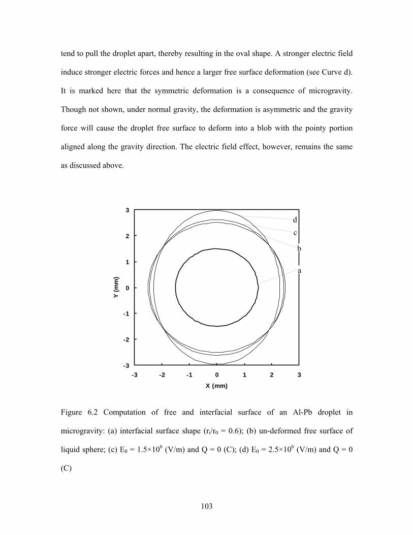
103

tend to pull the droplet apart, thereby resulting in the oval shape. A stronger electric field

induce stronger electric forces and hence a larger free surface deformation (see Curve d).

It is marked here that the symmetric deformation is a consequence of microgravity.

Though not shown, under normal gravity, the deformation is asymmetric and the gravity

force will cause the droplet free surface to deform into a blob with the pointy portion

aligned along the gravity direction. The electric field effect, however, remains the same

as discussed above.

-3

-2

-1

0

1

2

3

-3 -2 -1 0 1 2 3

X (mm)

Y (m

m)

Figure 6.2 Computation of free and interfacial surface of an Al-Pb droplet in

microgravity: (a) interfacial surface shape (ri/r0 = 0.6); (b) un-deformed free surface of

liquid sphere; (c) E0 = 1.5×106 (V/m) and Q = 0 (C); (d) E0 = 2.5×106 (V/m) and Q = 0

(C)

a

b

c d

104

6.2.2 Steady-state temperature and flow fields

As stated earlier, the Maxwell stress only has a component normal to the surface of the

droplet and is zero inside. Because it is non-vortical in nature, the stress does not induce

internal flow in the droplet. However, the laser heating of the droplet generates a non-

uniform temperature distribution both inside and along the surface of the droplet. This

temperature variation along the free surface and the interface of the two immiscible fluids

gives rise to a non-uniform thermocapillary forces that drive the recirculating fluid flows

in both liquids.

Fig. 6.3 summarizes the possible different thermal and flow patterns inside the

immiscible droplets electrostatically positioned in microgravity. Here A-B (e.g. Si-Co)

means that the outer layer of the droplet is A (i.e. Si) and the inside core is A (i.e. Co);

this convention will be used hereafter unless otherwise indicated. The droplet shapes are

calculated based on the condition given in Table 6.2. The deformation of the droplet is a

result of balance between the electric and surface tension forces along the droplet surface,

which differs from droplet to droplet, as shown in Fig. 6.3. The temperature and the

velocity distributions along the free surface and along the immiscible interface are shown

in Figs. 6.4 and 6.5 respectively.

Analyses are made to understand the underlying physics that governs these

complex thermal and fluid field distributions in these droplets. Let us start with the

thermal fields. A feature common to these cases is that the temperature field is symmetric

with respect to the equator plane, a mere consequence of the laser beams being applied at

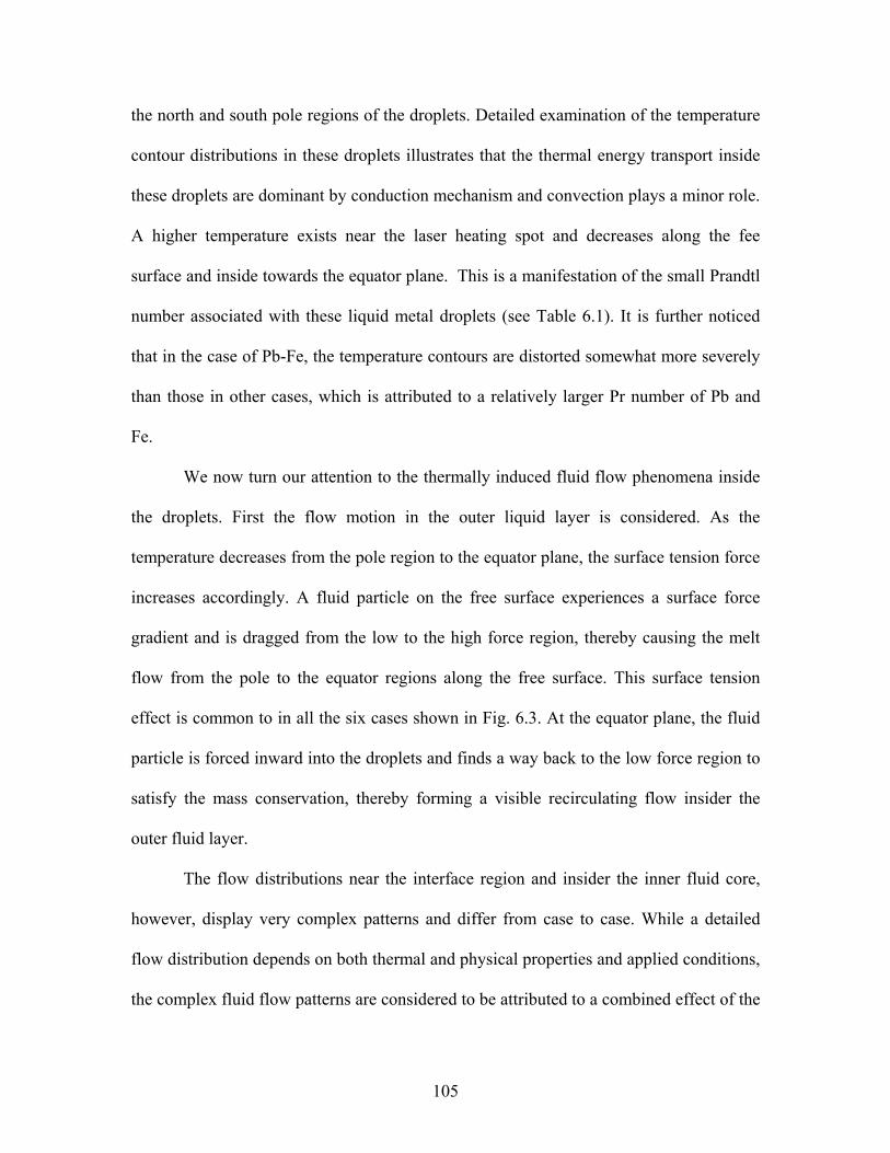
105

the north and south pole regions of the droplets. Detailed examination of the temperature

contour distributions in these droplets illustrates that the thermal energy transport inside

these droplets are dominant by conduction mechanism and convection plays a minor role.

A higher temperature exists near the laser heating spot and decreases along the fee

surface and inside towards the equator plane. This is a manifestation of the small Prandtl

number associated with these liquid metal droplets (see Table 6.1). It is further noticed

that in the case of Pb-Fe, the temperature contours are distorted somewhat more severely

than those in other cases, which is attributed to a relatively larger Pr number of Pb and

Fe.

We now turn our attention to the thermally induced fluid flow phenomena inside

the droplets. First the flow motion in the outer liquid layer is considered. As the

temperature decreases from the pole region to the equator plane, the surface tension force

increases accordingly. A fluid particle on the free surface experiences a surface force

gradient and is dragged from the low to the high force region, thereby causing the melt

flow from the pole to the equator regions along the free surface. This surface tension

effect is common to in all the six cases shown in Fig. 6.3. At the equator plane, the fluid

particle is forced inward into the droplets and finds a way back to the low force region to

satisfy the mass conservation, thereby forming a visible recirculating flow insider the

outer fluid layer.

The flow distributions near the interface region and insider the inner fluid core,

however, display very complex patterns and differ from case to case. While a detailed

flow distribution depends on both thermal and physical properties and applied conditions,

the complex fluid flow patterns are considered to be attributed to a combined effect of the

106

interfacial thermocapillary forces and the inertia in the outer fluid layer. Similar to the

Marangoni force on the free surface, the interfacial thermocapillary force increases also

with a decrease in temperature along the interface and pulls the fluid steam from the high

to the low temperature region (see Figs. 6.4b and 6.5b). The interfacial force acts as a

momentum source that drives the flow in both fluids. Other the other hand, the flow

resulting from the free surface Marangoni force produces an inertia that superimposes the

interface and counterbalances the effect from the thermocapillary force. It is this

competing mechanism that drives the flow near the interface and the flow inside the core

of the droplet.

In the case of Al-In, a strong flow driven by the free surface Marangoni force

provides a strong inertia near the immiscible interface and almost completely overpowers

the interfacial thermocapillary force, thereby resulting in a very weak flow in the inner

fluid core (see Fig. 6.3a). Exchanging the inside and outside fluids gives rise to a weaker

flow is generated in the outer layer. Thus a visible recirculating flow appears in the inner

fluid (see Fig. 6.3b and Fig. 6.5). Perhaps, this competing mechanism for the internal

flows is most revealing in the results shown in Fig. 6.3c. There are four strong

recirculating eddies that comprise the entire flow field, with two in the outer and two in

the inner fluids. The largest and yet strongest eddy occurs in the outer layer near the

equation, which is driven by the free surface Marangoni forces. The eddy in the inner

fluid near equator is clearly the consequence of the inertia force dominating the

interfacial surface tension effect. In the region near the immiscible interface from the pole

(θ= ±π/2) to (θ= ± π/4), the interfacial surface gradient shows its strongest effect and

overpowers the inertia force from the outer fluid layer. It provides the major momentum

107

force that drives the two recirculating loops in the region. When the two fluids switched

in positions in the droplet, the interfacial surface force gradient becomes even more

effective in driving the fluid motion near the immiscible interface. This is evident in Fig.

6.5 (d) in that the inner fluid is now completely covered by one eddy, which is apparently

a consequence of the interfacial force induced eddy engulfing the weak inner flow eddy

from near the equator plane. The same can be said for the thermal and fluid flow fields in

Figs. 6.3f and 6.3e, respectively. As expected, this competing mechanism between the

interfacial surface force gradient and outer flow inertia can cause a variety of different

flow conditions.

The flow pattern, velocity intensity and thermal field distribution inside the

droplets depend upon various parameters, as discussed above. These fluid dynamics and

thermal characteristics are also affected by the ratio of the outer and inner fluid volumes.

Two of these cases are shown in Fig. 6.6 for the Si-Co immiscible melt droplets with two

different volumes of fluids. Comparison of Fig. 6.6 with Fig. 6.3(e) shows that the

interfacial thermocapillary force becomes much stronger when the inner radius over ratio

is reduced. Indeed, Fig. 6.6(a) suggests that the flow insider the inner fluid shows an

overwhelmingly strong effect from the interfacial surface tension gradient. This contrasts

with the case of Fig. 6.6(b), which shows that the effect of the interfacial thermocapillary

force is essentially suppressed by the momentum from the outer layer fluid, when the

inner-outer radius ratio is reduced to 0.4. This effect is obviously attributed to the fact

that a much higher surface temperature gradient exists along the immiscible interface,

because of the improved heat conduction due to the increased ratio of the inner over outer

radius.

108

Parameters Al-ln ln-Al Fe-Pb Pb-Fe Co-Si Si-Co Si-Co Si-Co E×10-6 (V/m) 2.5 1.0 2.5 1.5 2.5 2.0 2.0 2.0

Q0×10-5 (W/m2) 1.0 1.0 11 11 10 10 10 10

ad (mm) 2.5 2.5 2.5 2.5 2.5 2.5 2.5 2.5 al (mm) 1.85 1.85 1.85 1.85 1.85 1.85 1.85 1.85 adi / ado 0.6 0.6 0.6 0.6 0.6 0.6 0.9 0.4

Vmaxo (outer surface) (cm/s) 2.44 0.89 7.72 9.17 7.01 5.69 3.90 6.15

Vmaxi (inner surface) (cm/s) 0.32 0.22 2.48 3.74 2.68 2.36 3.00 1.09

∆T K (outer surface) 1.40 2.60 16.20 59.90 11.8 8.90 10.3 8.80 ∆T K (inner surface) 0.47 0.58 7.32 8.89 3.24 3.06 7.64 1.33

Mai 3.82 3.82 69.73 69.73 18.39 18.39 72.28 12.58 Mao 25.45 13.41 264.9 529.8 164.8 58.45 67.12 57.34 Reo 111.9 82.68 246.2 923.7 323.8 379.8 260.3 410.5

Table 6.2 Parameters and some calculated results

(a) Al-ln (b) ln-Al

109

(c) Fe-Pb (d) Pb-Fe

(e) Si-Co

(f) Co-Si

Figure 6.3 Steady-state fluid flow and temperature distribution in the droplet (ri / ro = 0.6)

for some immiscible materials.

110

0

10

20

30

40

50

60

-1.57 -0.785 0 0.785 1.57

Si-CoCo-Siln-AlAl-lnPb-FeFe-Pb

(a)

0

1

2

3

4

5

6

7

8

9

-1.57 -0.785 0 0.785 1.57


(b)

Figure 6.4 Steady state temperature distribution (∆T = T-Tsmin, where Tsmin is the

minimum surface temperature) along the free surface (a) and the interface between the

θ

θ

∆T

∆T

111

two immiscible liquid metals (b). The surface is measured from south (θ = -π/2) to north

(θ = π/2) pole.

-10

-8

-6

-4

-2

0

2

4

6

8

10

-1.57 -0.785 0 0.785 1.57


(a)

-4

-3

-2

-1

0

1

2

3

4

-1.57 -0.785 0 0.785 1.57


(b)

θ

θ

v (cm/s)

v (cm/s)

112

Figure 6.5 Steady state fluid flow distribution along the free surface boundary (a) and the

interface between the two immiscible liquid metals (b). The angle θ is measured from (θ

= -π/2) to (θ = π/2). The velocity is positive in the clockwise direction and negative in the

anti-clockwise direction

(a) ri / ro = 0.9

(b) ri / ro = 0.4

Figure 6.6 Steady-state fluid flow and temperature distribution in the Si-Co droplet with

different radius ratios

6.2.3 Evolution of fluid flow and temperature fields

Knowledge of the decay of both temperature and velocity fields in a levitated droplet of

the immiscible metals, as it cools into an undercooling region, is crucial for the design of

microgravity experiments with the droplet. In practice, when the levitation is stabilized

113

and the sample is heated to a desired temperature, the laser beams are turned off and the

sample is allowed to cool below the melting point of one of the two fluids by radiation.

The computational methodology discussed above may be applied to predict the dynamic

development of transient thermal and fluid flow fields in electrostatically positioned

droplets as they undergo undercooling. The Pb-Fe droplets are selected for discussion in

this study, and the analysis should be applicable to other cases well.

Fig. 6.7 illustrates a set of snap shots of the time evolving velocity and

temperature fields in the Pb-Fe droplet when the laser power is switched off and the

droplet is allowed to cool for about 3 seconds. At this point, the temperature drops below

the melting point of iron. The calculations began with the initial (t=0) velocity and

temperature fields shown in Fig. 6.3 (d). The time development of the detailed

temperature and velocity distributions both along the free surface and the immiscible

interface are shown in Figs. 6.8 and 6.9. The two-fold symmetry with respect to the

equator plane is apparently a consequence of the initial fields and thus does not need an

elaboration.

Cross-examination of Figs. 6.7 to 6.9 reveals some of most interesting features

associated with this complex evolving thermal and fluid flow phenomena as the droplet

cools into the undercooling region. First, the temperature drops very rapidly over t=0 to

t=0.1 (sec) after the laser power is turned off and the decrease continues afterwards but at

a slower pace. At t = 0.1 (sec), the outer surface temperature difference at the pole

(θ=±π/2) has decreased by about 30 times, which compares with a factor of 5 for a drop

in the inner temperature difference at θ=±π/2 (also see Fig. 6.4). On the free surface, the

temperature gradient is completely reversed at about 0.2 (sec) in that the temperature at

114

the pole becomes smaller than that at the equator. In comparison, the reversal takes about

0.3 (sec) along the immiscible interface. After the reversal completes, the temperature

gradient direction remains the same along both the free surface and the interface. Again,

this dynamic evolution of the thermal field is by conduction and surface radiation, and

the convection effect is relatively weak or minimal, as evident by the small Prandlt

number of the melts. As thermal radiation is stronger near the pole where temperature is

high, the temperature reversal starts there. This change in the thermal field is responsible

for the complex evolving fluid flow field in the droplet, as shown in Fig. 6.7.

Fig. 6.7a shows that at t=0.1 (sec), the four-loop structure remains unchanged

despite a significant drop in temperature. This is because the surface tension force

gradient is unchanged. The large drop in the temperature, however, is reflected in the

velocity magnitude, as is evident by comparing Fig. 6.6 and Fig. 6.9, where the velocity

distribution along the free and inter surfaces are plotted. At some time close to t=0.2

(sec), the temperature gradient along the free surface is reversed such that the temperature

at the equator plane becomes higher than that at the pole. This change in temperature

gradient causes a corresponding reversal of the surface tension force gradient, with a

higher pulling force now at the pole. Consequently, the fluid stream along the free surface

flows from the equator plane to the poles (see Fig. 6.7b), which causes the outer fluid

eddy near the equator to reverse its rotation. At this point, however, the interfacial surface

force gradient still is the same as before, and intends to drive the flow from the pole to

the equator region. Thus, in the near interfacial region, the outer flow inertia force

complements the interfacial surface force gradient, thereby giving rise to the fluid pattern

as shown in Fig. 6.7b. As the evolution continues, the interface gradually completes its

115

temperature reversal. Then the inertia force starts competing with the interface surface

force in driving the fluid flow near the interfacial region. Figs. 6.7c and 6.7d reveal that

the outer flow inertia force becomes more powerful from t = 0.3 (sec) onwards and drives

the flow near the immiscible interface region. This means that the flow in both the

immiscible fluids of the droplet comes primarily from the free surface Marangoni effect

and the interfacial surface force has a negligible role.

6.3 Concluding remarks

This chapter has presented a numerical study of the free surface deformation and

Marangoni convection in immiscible droplets electrostatically positioned under

microgravity. The computational methodology employs the boundary element method

for the solution of the electrostatic field outside the conducting droplet and couples with

the weighted residuals method for solving the unknown free surface shapes along the free

surfaces. With the droplet fee surface shapes determined, the temperature and fluid flow

fields are solved using the Galerkin finite element method. Both the transient and steady

state thermal and fluid flow fields are solved, with the implicit backward Euler scheme

used for the time matching. Analyses show that the inner interface demarking the two

immiscible fluids in an electrically conducting droplet is immune to the applied

electrostatic field and maintains its sphericity in microgravity. The free surface or the

outer surface, however, deforms into an oval shape and its equilibrium shape is

determined by the balance of the Maxwell stress and the surface tension. The deformation

is caused by the pulling action of the electric forces resulting from the interaction of the

116

induced charges and the applied electric field. The thermal and fluid flow distributions

are rather complex in an immiscible droplet. The dominant mechanism for thermal

transport in the droplet is heat conduction and convection plays only a minor role. The

flow near the free surface is driven by the well-known Marangoni convection

mechanism, which causes the fluid particle to move from the high to low temperature

regions. The flow inside the inner fluid and near the immiscible interface, however, is

driven by a competing mechanism between the thermally induced interfacial surface

tension gradient and the inertia force in the outer fluid layer induced by the free surface

Marangoni convection. During cooling into an undercooled state after the laser hearting

is switched, the surface temperature gradients, both along the free surface and the

immiscible interface, experience a reversal, which is caused by surface radiation. This

reversal in the temperature gradients results in a reversal of the surface flow. During the

time between the surface thermal gradient reversals along the free and the interfacial

surfaces, the flow near the interfacial region may be driven by a complimentary

mechanism between the interfacial and the inertia forces during the thermal and fluid

flow transitional period. Before and after the completion of the interfacial thermal

gradient reversal, however, the interfacial flows are driven by the competing mechanism

between the interfacial and inertia forces, with the latter overwhelmingly dominating

after the thermal reversal is completed along both the free and interfacial surfaces.

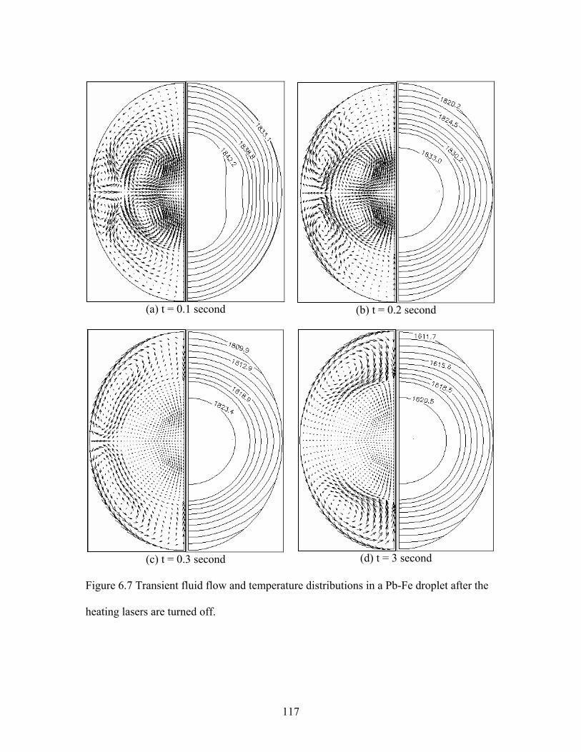
117

(a) t = 0.1 second

(b) t = 0.2 second

(c) t = 0.3 second

(d) t = 3 second

Figure 6.7 Transient fluid flow and temperature distributions in a Pb-Fe droplet after the

heating lasers are turned off.

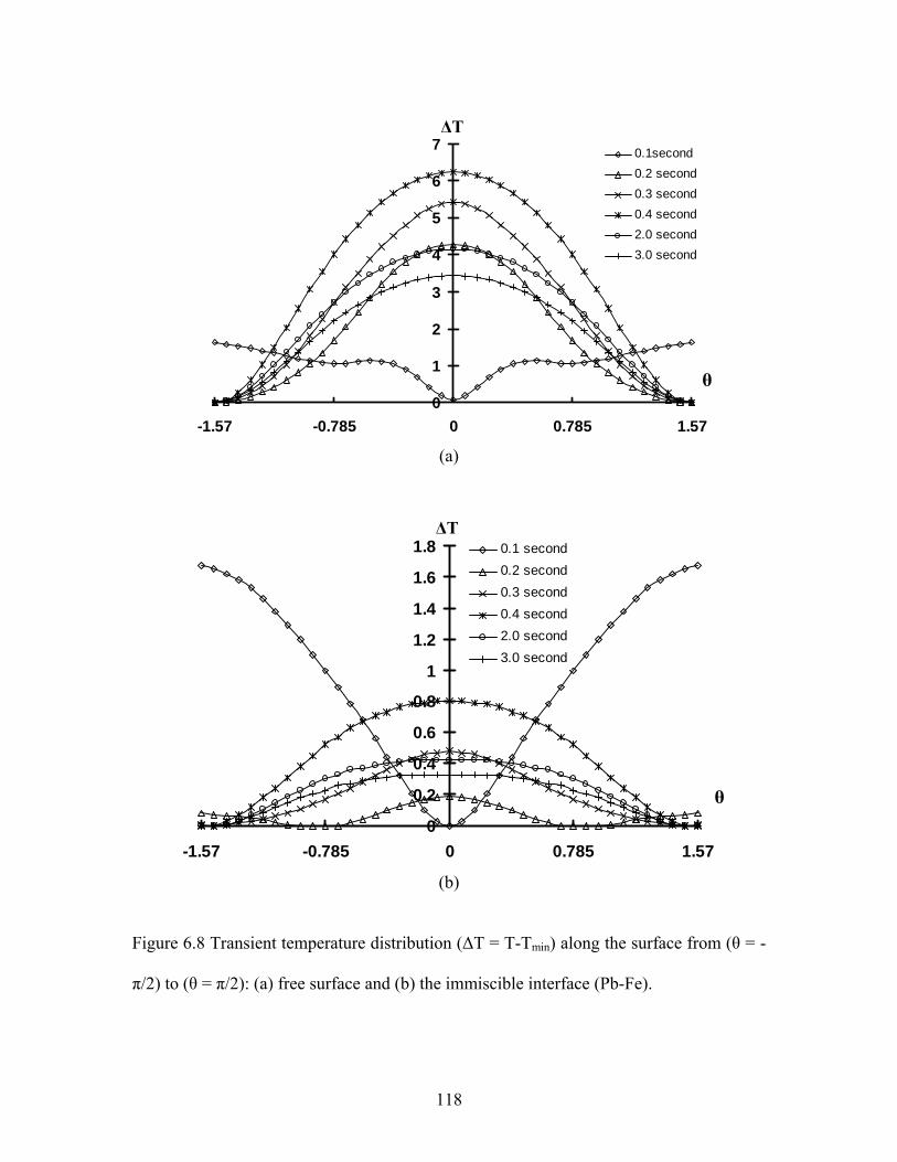
118

0

1

2

3

4

5

6

7

-1.57 -0.785 0 0.785 1.57

0.1second0.2 second0.3 second0.4 second2.0 second3.0 second

(a)

0

0.2

0.4

0.6

0.8

1

1.2

1.4

1.6

1.8

-1.57 -0.785 0 0.785 1.57

0.1 second0.2 second0.3 second0.4 second2.0 second3.0 second

(b)

Figure 6.8 Transient temperature distribution (∆T = T-Tmin) along the surface from (θ = -

π/2) to (θ = π/2): (a) free surface and (b) the immiscible interface (Pb-Fe).

∆T

θ

θ

∆T

119

-3

-2

-1

0

1

2

3

-1.57 -0.785 0 0.785 1.57


(a)

-2.5

-2

-1.5

-1

-0.5

0

0.5

1

1.5

2

2.5

-1.57 -0.785 0 0.785 1.57


(b)

Figure 6.9 Transient fluid flow distribution along the surface from (θ = -π/2) to (θ = π/2):

(a) free surface and (b) the immiscible interface (Pb-Fe). The velocity is positive in the

clockwise direction and negative in the anti-clockwise direction

θ

θ

v (cm/s)

v (cm/s)

120

CHAPTER 7

2-D FEM/BEM SIMULATION OF THE OSCILLATION OF THE

ELECTROSTATICALLY LEVITATED DROPLET

7.1 Introduction

In this chapter, a mathematical model is developed for the oscillation of the

electrostatically levitated droplet under microgravity. The computational methodology

entails solving the Laplace equation by the boundary element method, solving the

Navier-Stokes equations by the Galerkin finite element method, and the use of deforming

elements to track the oscillating free surface shapes. The pressure-velocity formulation is

used in the finite element model for the internal fluid flow. To incorporate the free

surface kinematical boundary condition, the front tracking technique is applied. The

electric fields, surface driven flow fields and deformed surface shapes are calculated

iteratively for each time step during drop oscillation. Computed results are presented for

both free surface oscillations and internal fluid flows in electrostatically positioned

droplets in microgravity environment. The effect of both the electric field and the surface

tension on the frequency of the oscillation is studied. The effect of the viscosity on the

damping constant is also analyzed.

7.2 Problem Statement

121

Figure 7.1 Schematic representation of an initial (dash line) and steady-state for the

computation of the electrostatically levitated droplet

Figure 7.1 shows the initial and steady state positions in the oscillation of the

electrostatically levitated droplets. A complete description of the electrically induced

surface oscillation and pressure fluid flow phenomena in a droplet requires the solution of

the coupled Maxwell and Navier-Stokes equations. At present, the Maxwell equation is

simplified to a partial differential equation governing the distribution of the electric field

outside the droplet. The buoyancy effects being neglected for microgravity applications,

the equations for the electric and fluid flow may be written as follows,

02 =Φ∇ 2Ω∈ (7.1)

0u =⋅∇ 1Ω∈ (7.2)

2Ω1Ω

122

( ) surfaceT Fp

t+∇+∇⋅∇+−∇=∇⋅+

∂∂ )u(uuuu ηρρ 1Ω∈ (7.3)

The solution of above electric field and fluid flow equations may be obtained by applying

the appropriate boundary conditions, which are stated below

0Φ=Φ 21 Ω∩Ω∈ (7.4)

eσε −=Φ∇⋅n0 21 Ω∩Ω∈ (7.5)

Qdsdse =Φ∇⋅−= ∫∫∫∫ΩΩ

n11

0∂∂

εσ 21 Ω∩Ω∈ (7.6)

θcos0RE−=Φ ∞→R (7.7)

nTnnn ⋅⋅−⋅⋅= EsurfaceF σ 21 Ω∩Ω∈ (7.8)

γσ H2=⋅⋅ nn 21 Ω∩Ω∈ (7.9)

Φ∇= 2

21 εET 21 Ω∩Ω∈ (7.10)

0XudtdX

=∇⋅+ 21 Ω∩Ω∈ (7.11)

01

VdV =∫Ω 21 Ω∩Ω∈ (7.12)

czdVz =∫Ω1

21 Ω∩Ω∈ (7.13)

In the above, Eq. (7.5) is the jump condition for the electric field along the droplet

surface, a manifestation of a well known fact that charges are distributed only on the

surface of a conducting body. Eq. (7.7) describes the electric potential condition at

123

infinity. The law of charge conservation is described by Eq. (7.6), where Q is the total

free charge applied on the droplet, which is zero for the problem under consideration for

microgravity applications. Eq. (7.8) describes the force induced by the Maxwell and

surface tension stresses along the normal direction. In Eq. (7.9), σ is the stress tensor, γ

is the surface tension and H is the Gaussian mean curvature. Eq. (7.10) describes the

Maxwell stress associated with the electric potential. Eq. (7.11) is the kinematic

condition, which describes the interface, represented by the X(xi,t)=0 always remains an

interface. The constraints of the volume conservation (Eq. (7.12)) and the center of the

mass (Eq. (7.13)) of the electrostatically levitated droplet are needed to determine the

shape and position of the droplet.

7.3 Method of Solution

7.3.1 BEM solution of the electric potential

The numerical solution of the electric potential equation (Laplace equation) along the free

surface boundary conditions is obtained by applying the BEM. We are seeking an

approximate solution to the problem governed by Eq. (7.1). The error introduced by

replacing Φ by an approximate solution can be minimized by writing the following

weighted residual statement:

∫∫ ∫ΓΩ Γ

ΓΦ−Γ=ΩΦ∇ )(),()()(),()()(),()( *2

2

rdrrqrrdrrGrqrdrrGr iii (7.14)

124

where G is interpreted as a weighting function and

)(

),(),(*

rnrrGrrq i

i ∂∂

= (7.15)

After some transformation, we can get the final form used for the BEM simulation.

ΓΦ∇⋅+ΓΦ∇⋅

=Γ∇⋅Φ+Γ∇⋅Φ+Φ

∫∫

∫∫

ΩΩ

ΩΩ

drGdrG

rdGrdGrrC ii

22

22

)'()'(

)(')(')(')(

∂∂

∂∂

nn

nn

(7.16)

where

⎪⎪⎪

⎩

⎪⎪⎪

⎨

⎧

−−

=

;2

2

;21;1

)(

21

πββπ

irC

and Φ’ = Φ + Ercosθ, ∂Ω2 designates the surface of the droplet and 2Ω∂ denotes the

boundary at infinity. The Green function, G, and its normal derivative are calculated by

the following expressions written for a cylindrical coordinate system [Jackson, 1975].

( ) ( )

)(4),(22

κKzzrr

rrGii

i−++

= (7.17)

when ri lies inside domain

when ri lies on a smooth domain

when ri lies on a nonsmooth domain

125

( ) ( )

( ) ( )[ ]( ) ( )

⎪⎪⎭

⎪⎪⎬

⎫

⎪⎪⎩

⎪⎪⎨

⎧

−+−−+−

−−

−++=

)()()(

24

22

22κ

κκ

∂∂

Ezzrr

zznrrn

KEr

n

zzrrnG

ii

izir

r

ii

(7.18)

where κ is the geometric parameter calculated by

222

)()(4

zzrrrr

ii

i

−++=κ (7.19)

The function G and Φ’ have the following asymptotic properties,

)(),(' 2−≈Φ RORri , )(),(' 3−≈Φ RORrn i∂

∂ as ∞→R (7.20)

)(),( 2−≈ RORrG i , )(),( 3−≈ RORrnG

i∂∂ as ∞→R (7.21)

Also dΓ = R(θ) dθ. Thus, the two integrals each approach zero as R → ∞ ,

0)('2

→Γ∇⋅Φ∫Ω∂

rdGn and 0)'(2

→ΓΦ∇⋅∫Ω∂

rdG n as ∞→R (7.22)

Thus, Eq. (7.16) simplifies to a boundary integral that involves only the surface of the

droplet, ∂Ω2. Following the standard boundary element discretization, noticing that the

potential on the surface is a constant and substituting Φ = Φ’ - Ercosθ into the resultant

126

equation, one obtains the final matrix form for the unknowns on the surface of the

droplet,

zEnzE

nHGGH −

⎭⎬⎫

⎩⎨⎧+

⎭⎬⎫

⎩⎨⎧ Φ

−=Φ∂∂

∂∂

0 (7.23)

where H and G are the coefficient matrices involving the integration of ∂G/∂n and G over

a boundary element. To complete the solution, Eq. (7.6) is discretized and solved along

with the above equation to obtain the surface distribution of ∂Φ/∂n and the constant Φ0.

7.3.2 FEM solution of the fluid flow and free surface movement

The transport equations for the internal fluid flow along with the boundary conditions are

solved using the Galerkin finite element method. The continuity and N-S equations with

the pressure-velocity formulation can be discretized as follows,

0U)/ˆ(1

2 =⎟⎟⎠

⎞⎜⎜⎝

⎛Ω+∇⋅∫

Ω

iTi

T dri φδφψ (7.24)

∫∫

∫∫

∫∫∫

Ω∂Ω∂

ΩΩ

ΩΩΩ

Γ⋅⋅−Γ⋅⋅

=⎟⎟⎠

⎞⎜⎜⎝

⎛Ω∇⋅∇⋅+⎟

⎟⎠

⎞⎜⎜⎝

⎛Ω⋅+∇⋅∇

+⎟⎟⎠

⎞⎜⎜⎝

⎛Ω+∇⋅−⎟

⎟⎠

⎞⎜⎜⎝

⎛Ω∇⋅+

∂∂

⎟⎟⎠

⎞⎜⎜⎝

⎛Ω

11

11

111

ˆnˆn

U)ˆ)(ˆ(U)/2(

P)/ˆ(UuU

22

2

diTdi

djidr

dridt

d

E

iTiTi

T

Ti

iTi

T

φφσ

φφηφφδφφη

ψφδφφρφρφφ

(7.25)

127

where U is a global vector containing all nodes values of u and v, and P the global vector

containing the nodal values of pressure. Once the form of the shape functions is specified,

the integrals defined in the above equations can be calculated numerically. It is noted that

the selection of the shape functions must satisfy Babuska-Brezzi condition. The

discretized momentum and energy equations may be combined into a single global matrix

equation,

⎥⎦

⎤⎢⎣

⎡=⎥

⎦

⎤⎢⎣

⎡⎥⎦

⎤⎢⎣

⎡−

−++⎥

⎦

⎤⎢⎣

⎡⎥⎦

⎤⎢⎣

⎡0F

PU

0CCKA(U)

PU

000M

T&

& (7.26)

where the coefficient matrices in the above equation are defined by,

∫Ω

Ω=1

M dTρφφ ; ∫Ω

Ω+∇⋅=1

)/ˆ( 2 drjC Tjj ψφδφ ;

∫Ω

Ω∇⋅=1

uA(U) dTφρφ ; ∫∫Ω∂Ω∂

Γ⋅⋅−Γ⋅⋅=11

ˆnˆnF diTdi Ei φφσ ;

⎟⎟⎠

⎞⎜⎜⎝

⎛Ω∇⋅∇⋅+⎟

⎟⎠

⎞⎜⎜⎝

⎛Ω⋅+∇⋅∇= ∫∫

ΩΩ 11

)ˆ)(ˆ()/2(K 22 djidr T

ijT

iT

ij φφηδφφδφφη

where j = 1, 2 and ijδ is a delta function. The assembled global matrix equations are

stored in the skyline form and solved using the Gaussian elimination method. For free

surface problem, F has a contribution from the normal stress balance, which my be

further simplified by the theorem of differential geometry.

128

∫∫∫∫∫Γ∂ΓΓΓΓ

Γ⋅+Γ⋅∇−=Γ⋅∇=Γ=Γ⋅⋅fffff

dddHdd SS nmnnnn kkkkk φφφγφσφ (7.27)

where S∇ is the surface gradient operator, fΓ is the free surface or boundary, fΓ∂ is the

bounding curve for the free surface and m is the normal to fΓ∂ but tangential to fΓ .

To incorporate the free surface kinematric boundary condition, the front tracking

technique is applied, By this techniques, the nodes along the free surface are allowed to

move such that they remain on the oscillating surface all the time. Thus, Eq. (7.12) can be

solved using the Weighted Residuals Methods (WRM) with the result,

0X)udtdX( =Γ∇⋅+∫

Γ f

dχ (7.28)

where χ is the shape function for the free surface coordinates. Discretization, followed

by numerical integration and assembly, gives rise to the following matrix equation,

0XKXM =+& (7.29)

where M and K are global matrices for free surface coordinates. Because the nodes of

the free surface are allowed to move to satisfy Eq. (7.29), these movement must be

superimposed on the velocity at the nodal points and therefore the convection term in Eq.

129

(7.3) must be modified accordingly, that is, uu ∇⋅ρ is replaced by u)uu( s ∇⋅+ρ where

us is the nodal velocity due to the free surface movement.

7.3.3 Numerical procedures

The solution of the above equations defining the droplet oscillation in the electrostatic

levitation mechanism requires an iterative procedure. The required nonlinear iterations

are preformed using the successive substitution scheme method. The time derivatives are

approximated by the implicit finite difference scheme, with automatic time step control.

The iterative procedure starts with an initial condition for the free surface shape. With the

initial condition, the electric potential on the free surface is calculated by using BEM.

The fluid flow is then calculated with the updated Maxwell stress and the free surface

coordinates. The updated free surface is used to start another set of calculations for the

updated electric potential. The iterative procedure continues until all of the variables

converge within a preset tolerance. The convergence criterion for the calculations is set

such that the relative error between the two consecutive iterations is within 1×10-4.

7.4 Analytical Solutions from Other Researchers

Lord Rayleigh (1882) first derived the formula 21

320 )/2( ρπγ af = for the

fundamental vibrational frequency, where a is the radius of the droplet, ρ the density of

the droplet, and γ the surface tension. Experimental studies showed that the fundamental

vibrational frequency agreed well with the formula derived by Lord Rayleigh. Taylor

130

(1964) demonstrated that the equilibrium drop shape was aspherical and might be

approximated by a prolate spheroid. In his study, the equilibrium equations were satisfied

at the poles and the equator. For the droplet in a uniform electric field E0, Taylor derived

the following formulation,

IMaE )()8( 21

21

21

0 απγ =−

(7.30)

where

21

23

21

32

)2()( αααα −−=M ;

2)/( sl aa=α

where la is the semi-major axis and sa is the semi-minor axis for prolate spheroid as

1// 2222 =+ sl ayax . He concluded that the onset of instability occurs when

625.1)/( 2/10 =γRE and the deformation, expressed as the ratio sl aa / of the semi-major

and semi-minor axis of the drop is equal to 1.86.

Based on the assumption of spheroidal oscillatory shapes, the characteristic

frequency of the two-lobed mode for an uncharged conducting drop in a uniform electric

field was shown to decrease as the applied electric field strength increases [Rosenkilde

1969; Brazier-Smith et al. 1917]. In Smith’s study, the fundamental frequency of an

uncharged drop in a uniform electric field may be written as follows,

131

21

3 )2(1ρ

γπ r

xf = (7.31)

where

)2/1(

)12(3)1(2

3)11ln(

49

22

811

817 2

2

242

αα

αααα

+

−−⎥⎦

⎤⎢⎣

⎡−

−−

−+

−−+=

−−−−

aee

eeI

e

x

2)/( sl aa=α

21

2 ))(1(l

s

aae −=

Therefore, we can find the relation between frequency f and surface tension γ . Since the

relation between α and E0 is known, as shown in Eq. (7.30), the variation of f with E0

can be found.

Later on, the equilibrium shapes and the stability of a charged conducting drop

levitated by a uniform electric field were analyzed by Adornato and Brown (1983) whose

asymptotic and numerical analysis for the equilibrium drop shape in small electric fields

showed the appearance of second and third Legendre functions. Feng and Beard (1990)

further studied the nature of the axisymmetric oscillation of electrostatically levitated

droplets by using an analytic multiple parameter perturbation method. In Feng and Bear’s

study, the oscillatory response at each frequency consists of several Legendre

132

Polynomials rather than just one, and the characteristic frequency for each axisymmetric

mode decreases from that calculated by Rayleigh for stronger applied electric field. Feng

and Beard’s frequency correction term for axisymmetric n=2 may be written as,

)],,(1[20

2 eqFff γ−= (7.32)

where

64223

2422

227120176)54.114.6331.243(),,(

qqqeqqeqF

−+−+−

=γγγ

γγγ

0

22

22

16 επ rQq s=

02

02 εrEe =

sQ is the electric charge induced into the droplet, E0 is the uniform electric field, and 0ε

is the electric permittivity in the free space.

7.5 Numerical Results and Discussion

The computational methodology described above can be applied to predict the

distribution of electric potential, free surface oscillation and viscous flow in the

electrostatically positioned droplets. Because of limited space, a few computed results are

presented here from extensive numerical simulations. The calculation used 20 quadratic

133

boundary elements in half-circle model to calculate the electric potential fields, while 175

9-node finite elements in the quarter-circle model were employed for the computation of

fluid flow and free surface oscillations, as shown in Fig. 7.2. The criterion for the

convergence of non-linear iteration is set to 4101 −× (norm-2 relative error).

(a) (b)

Figure 7.2 Boundary element and finite element meshes: (a) boundary element mesh for

the computation of the electric potential, (b) finite element mesh for the computation of

the fluid flow and free surface oscillations

Since Lord Rayleigh (1882) first calculated the characteristic frequencies for

small-amplitude oscillations of a charged drop in the absence of external fields about the

spherical shape, the study of the droplet in the electric field has received a wide

interesting. Most of the studies focus on the analytical method except that Adornato and

134

Brown (1983) used FEM compared with the analytical method to study the shape and

stability of the droplet elevated in the uniform electric field. At present, we analyzed the

oscillation of the droplet levitated in the uniform electric field by using the FE/BE

method. Fig. 7.3 depicts three computed positions (initial, steady-state and the minimum)

of the oscillation of a liquid Aluminum droplet in the uniform electric field (E0=2.0×106

v/m), whose properties is shown Table 7.1. It is assumed that the droplet is kept the

elongated prolate spheroid with 3105.2 −×=a m, 310553.3 −×=la m, 31007.2 −×=sa m,

and 716.1/ =sl aa at the initial time. Therefore, the computed oscillation of the droplet

levitated in the electric field is below the critical values derived by Taylor and satisfied

with the stability condition. In the electrostatic levitation mechanism, the elongated

spherical droplet is first dragged back to the steady state position along the axis direction

by the surface tension with the velocity of the poles increasing and enlarged at the

equator surface in order to satisfy the mass conservation. Then the droplet reaches the

steady-state prolate spheroid form, as described in chapter 4. Because of the effect of the

inertial force, the droplet will pass by the steady-state position. After passing by the

steady-state position, the electric force is larger than the surface tension and the moving

velocity of both poles is reduced, but it still keeps moving towards the center of the

droplet. Finally, the poles of the droplet reach the closest position to the center of the

droplet (the minimum position as shown in Fig. 7.3), in which position the surface

tension has the minimum value and the Maxwell stress has the maximum value so that

the deformation of the droplet will be reversed. In order to depict the effect of the

hydrodynamic force, the velocity distribution of the large amplitude of the droplet in one

period is shown in Fig. 7.4

135

-1.5

-1

-0.5

0

0.5

1

1.5

0 0.4 0.8 1.2

initial state

steady state

minimum state

Figure 7.3 Three position of the droplet in half period of the oscillation of the droplet in

the electric field (E0=1.0×106 V/m)

(a) t=1.9×10-3 s Vmax=23.47 cm/s (b) t=5.8×10-3 s Vmax=31.72 cm/s

136

(c) t=9.6×10-3 s Vmax=31.00 cm/s (d) t=13.6×10-3 s Vmax=24.96 cm/s

Figure 7.4 Oscillation of an electrostatically levitated, aluminum droplet under

microgravity conditions in one period, (a) 1/8 period, (b) 3/8 period, (c) 5/8 period, and

(d) 7/8 period. The initial diameter of the droplet is 5 mm, E0=1.0×106 (V/m), the initial

deformation of the droplet is like that in Fig. 7.3.

Parameters Al

ρ (kg/m3) 2385

µ ×103 (kg/m-s) 1.3

γ (N/m) 0.914

a (mm) 2.5

Table 7.1 Parameter used for the computation

137

Rosenkilde (1969) and Brazier-Smith et al. (1971b) found that the characteristic

frequency of the two-lobed mode for an uncharged conducting droplet in a uniform

electric field decreased as the applied electric field intensity increased. Feng and Beard

(1990) also investigated the oscillation characteristics of electrostatically levitated

droplets. In the present study, the effect of the frequency associated with variation of the

electric field and surface tension is investigated. The computed results are first compared

with Feng and Beard’s analytical solution. Fig. 7.5 depicts the change of the normalized

characteristic frequency of a conducting droplet with electrical field intensity. From Fig.

7.5, we can find that the frequency decreased with the electric field intensity becoming

stronger. As shown in Fig. 7.5, the numerical results agree very well with the analytical

prediction derived by Feng and Beard. The Maximum relative error is equal to 2.7%,

which occurs when the electric field intensity reaches 2.1×106 (v/m). Fig. 7.6 shows the

frequency of the oscillation of the droplet changes with the surface tension. The

frequency of the droplet is increasing with the surface tension becoming larger.

Compared with the Feng and Beard’s results, the numerical results are good. However,

the numerical curve is a little lower than the analytical curve in Fig. 7.6. The main reason

is that the analytical solution only includes the major 2nd mode and neglects the higher

order modes. If the higher order Legendre polynomials are included, the formulation of

the analytical method will become very complicated. Therefore, our numerical method

may provide more accurate and fast results than the analytical method.

138

0.8

0.85

0.9

0.95

1

0 0.5 1 1.5 2 2.5

our numerical results

Feng's analytical results

Figure 7.5 Normalized characteristic frequency of a conducting droplet changed with

electrical field intensity E0 with 3105.2 −×=a m and 914.0=γ (N/m). The initial

deformation of the droplet is like that in Fig. 7.3

0

20

40

60

80

100

120

0 0.5 1 1.5 2 2.5 3

our numerical resultsFeng's analytical results

Figure 7.6 Characteristic frequency of a conducting drop changed with surface tension

Nor

mal

ized

freq

uenc

y

Electric field intensity E0 (×106 v/m)

Surface tension γ (N/m)

Freq

uenc

y

139

In the other researchers’ studies, the effect of the viscosity on the oscillation of

the droplet is neglected, such as Feng and Beard used the Bernoulli’s equation to describe

the pressure field p. In present study, the Navier-Stokes equation is solved every time

step and the effect of the viscosity is carried out. Fig. 7.7 shows the viscous decay of the

oscillation amplitude of droplet. Fig. 7.7 (a) and (b) respectively depict the viscous decay

of the oscillation amplitude without electric field and with electric field E0=1.0×106

(V/m). Fig. 7.7 (c) compares the result of (a) with that of (b), which shows that the

frequency with the electric field is smaller than that without the electric field. As shown

in Fig. 7.7, the frequency of the oscillation will keep unchanged with the decreasing of

the amplitude of the oscillation caused by the viscous effect. The numerical experiments

also describe that, unlike the electric fiend intensity and surface tension, the viscosity has

no effect on the frequency of the oscillation of the electrostatically levitated droplet. In

the present model, the damping constant τ is computed using the following equations,

)exp()2cos()()(τ

π tftaaata ll−

−+= (7.33)

where )(tal is the semi-major axis with time evolving, a is the radius of the spherical

droplet, and la is the semi-major axis at initial time. The damping constant τ is not

constant by using the current numerical model, which decreases with the time increasing.

This result indicates that the high order mode plays a significant role in the damping of

the oscillation.

140

0.6

0.7

0.8

0.9

1

1.1

1.2

1.3

1.4

1.5

0 0.02 0.04 0.06 0.08 0.1 0.12 0.14 0.16 0.18 0.2

Time (second)

Radi

us R

atio

(Rp/

a)

(a)

0.6

0.7

0.8

0.9

1

1.1

1.2

1.3

1.4

1.5

0 0.05 0.1 0.15 0.2 0.25 0.3Time (second)

Rad

ius

Rat

io (R

p/a)

(b)

141

0.6

0.70.8

0.9

11.1

1.2

1.31.4

1.5

0 0.05 0.1 0.15 0.2Time (second)

Rad

ius

Rat

io (R

p/a)

(c)

Figure 7.7 Viscous decay of oscillation amplitude ratio (divided by radius a) of the polar

point of the droplet, where a = 2.5 mm and the center presents the steady state position,

(a) oscillation without electric field, (b) oscillation with E0 = 1.0×106 (V/m), (c)

Comparison with (a) and (b).


In this chapter, a numerical study of melt droplet oscillation in electrostatic levitation

mechanism has been described. Numerical analysis is based on the solution of the electric

field by the boundary element method and the solution of the Navier-Stokes equations by

the finite element, together with the use of deforming elements to track the oscillating

free surface shapes. The computed result suggests that the frequency of the oscillation of

the electrostatically levitated droplet decrease with the electric field increasing and

increase with the surface tension increasing, which agrees with the prediction of the

: with electric field

142

analytic solution. The amplitude of the oscillation has no effect on the characteristic

frequency. The damping constant is affected significantly by the high order mode.

143

CHAPTER 8

STABILITY OF THE DROPLET IN THE MAGNETIC LEVITATION

MECHANISM

8.1 Introduction

This chapter presents a numerical study of the 3-D movement of the conducting spherical

droplet in the magnetic levitation mechanism. The present chapter not only investigates

the complex vertical and horizontal movement of the droplet, but also the self rotation of

the droplet. The hybrid 3-D boundary element method (BEM) and finite element method

(FEM) with edges elements are used to calculate electromagnetic fields, Lorentz force,

and torques with respect to the axis. By this method, finite elements are used to discretize

the spherical droplet region, while boundary elements are applied in the free space

outside the droplet region with the surface of the droplet. The finite element and

boundary element regions are then coupled through the interface boundary conditions.

The iterative coupling of the BEM and FEM is applied to calculate the electromagnetic

fields. The developed codes agree excellently with the available analytical and numerical

solutions. Further, the complex 3-D movement of the magnetically levitated droplet is

solved and analyzed by using the current FEM/BEM model.

8.2 Problem statement

144

13.5

9.5

10

4

4

Figure 8.1 Schematic representation of magnetic levitation System

Figure 8.1 shows the TEMPUS device in use [Song, 1998a, 1998b, 1999a]. The system

consists of two types of coils: (1) the inner four current loops (or heating coils) for

sample heating and melting, and (2) the outer eight loops (or positioning coils) for sample

positioning in space. During the operation, AC currents flow through these coils to

generate an appropriate magnetic field. In magnetic levitation, eddy currents are induced

in the sample and the dot product of eddy currents generates the Joule heating for the

melting of the sample. These eddy currents also interact with the applied and induced

magnetic fields to produce the Lorentz force in the sample. At present, we investigate the

effect of the Lorentz force on the sample’s 3-D movement in the magnetic levitation

mechanism.

8.2.1 Governing equations and boundary conditions for the computation of the

electromagnetic field

x

z

145

In order to calculate the distribution of electromagnetic fields in the specimen

surrounded by the exciting coils, the Maxwell’s equations have to be solved. However,

Maxwell’s equations are coupled partial differential equations, which have more than one

unknown variables. Therefore, the vector wave equation derived from the Maxwell’s

equations combined with the energy equation is taken as the governing equations to

simulate the microwave heating problems. With the analysis above, the equations for the

electric and thermal fields may be written as follows

icr

j JEE ωµµεωµ

−=−×∇×∇ 21 (8.1)

In the above, Ji is an impressed or source current, and εc (=ε-jσ/ω) results from the

combination of the induced current (σE) and displacement current (jωD). The appropriate

boundary conditions are stated below.

2221111

ˆˆ1 EnUUEn ×∇×==−=×∇×−rµ

21 Ω∩Ω∈ (8.2)

where Ω1 and Ω2 are the FEM domain, BEM domain respectively. 1n is outnormal from

the FE region, and 2n is outnormal from the BE region.

8.2.2 Governing equations and boundary conditions for the computation of the 3-D

movement of the droplet in the magnetic levitation mechanism

146

After the computation of the electromagnetic fields, the time-averaged

electromagnetic force induced in the sphere which is responsible for levitation as well as

for fluid motion, is the cross product of induced current and the complex conjugate of the

magnetic field,

)B(JRe21F ∗×=i (8.3)

it dV⋅×= ∗ )B(JRe21Fi (8.4)

iV

dV⋅= ∫ itotal FF (8.5)

where i is the element number. As the levitating motion, we considered the translation.

Therefore, the translation equations are introduced into this analysis. The Leap Frog

Algorithm is used. This algorithm evaluates the velocities at half-integer time steps and

uses these velocities to compute new positions.

t

ss nn

∆−

≡++ 1

21n

v (8.6)

tss nn

∆−

≡−− 1

21n

v (8.7)

So we can derive the new position, based on the old position and velocity:

21

n1n tvss++ ∆+=

n (8.8)

147

From the Verlet algorithm, we have the following expression for velocity:

n21n

21n

avv t∆+=++

(8.9)

m/Fa totaln n= (8.10)

where a is the acceleration, m is the weight of the metal, ∆t the width of time step, v the

velocity at center of the metal and s the position vector. The fluid flow and temperature

distribution may also be calculated at every time step.

After the time-averaged electromagnetic force is calculated, the torque with

respect to the axis may be written as follows,

tiitiN FR ×= (8.11)

∑=

=1

totalNi

tiN (8.12)

The rotating moving equations at every time step are given by,

nn ωωω ∆+=+ n1 (8.13)

nn θθθ ∆+=+ n1 (8.14)

with

148

mn I∆t /Ntotal=∆ω (8.15)

)2/(N 2total m

nn I∆tt +∆=∆ ωθ (8.16)

where Ri is the radius vector drawn from center to surface of a sphere metal, ω the

angular velocity, θ the rotational angle, and mI the moment of inertia. In the present

study, the droplet is assumed to be spherical without considering the deformation of the

droplet. Therefore, the moment of inertia mI may be written as,

2mR)5/2(=mI

where m is the weight of the droplet, R the radius of the spherical droplet.

8.3 Method of Solution

The 3-D electromagnetic field may be solved using the edge finite element method [Huo,

2004c, 2005b]. The edge-based elements are necessary to satisfy the divergence-free

constraint, ∇⋅E=0 [Johns, 1971]. However, the huge sparse matrix produced by the FEM

appears to be a major setback to finding an efficient numerical solution to a large scale

problem. Our experience shows that this remains true even with various efficient solvers

designed specifically for the solution of a large sparse system of linear algebraic

equations to improve the computational efficiency. To alleviate the disadvantage of the

finite element method, a hybrid finite element-boundary method is employed instead.

149

Using this approach, finite elements are used in the conducting droplet where power

density is needed and material properties may be a function of temperature, while

boundary elements are used elsewhere. The FEM and the BEM are coupled through the

interface boundary conditions. This idea is shown in Figure 8.2

Figure 8.2 Schematic representation of the coupling of the finite element and boundary

element

8.3.1 Finite element formulation

To develop a finite element formulation in the conducting droplet, the wave equation

(8.1) is integrated with respect to a vector testing function δE [Akarapu, accepted].

dVjdV iV

crV

E1E 2 δωµµεωµ

δ ⋅−=⎟⎟⎠

⎞⎜⎜⎝

⎛−×∇×∇⋅ ∫∫∫∫∫∫ JEE (8.17)

Integration by parts gives rise to the surface integral term,

Ω1

Ω2

Interface of FEM and BEM

Ω1: FEM Ω2: BEM

150

( ) dVjdS

dVdV

iVS r

Vc

V r

JnE

EE

∫∫∫∫∫

∫∫∫∫∫∫

⋅−⋅×∇×

=⋅−×∇⋅×∇

EE1

EE1 2

ωµδδµ

δµεωδµ

(8.18)

Making use of the vector identity

( ) ( ) EˆˆE δδ ⋅×∇×−=⋅×∇× EnnE (8.19)

and also the boundary conditions, the final integral formulation is obtained,

[ ] dVjdS

dV

iVS

Vc

r

JU

EE

∫∫∫∫∫

∫∫∫⋅−⋅−

=⎟⎟⎠

⎞⎜⎜⎝

⎛⋅−×∇⋅×∇

EE

EE1 2

ωµδδ

δµεωδµ (8.20)

With appropriate finite element discretization and necessary elemental calculations

followed by assembly, one has the matrix representation of equation (3.46),

F[B]U[K]E =+ (8.21)

where the matrix elements are calculated using the following expressions,

151

dVKV

jicjir

ij ∫∫∫ ⎟⎟⎠

⎞⎜⎜⎝

⎛⋅−×∇⋅×∇= NNNN µεω

µ21

dSBS

jiij ∫∫ ⋅= SN

dVjFV

i ii JN ⋅−= ∫∫∫ ϖµ

Note that here Ni and Si are edge-based vector shape functions and their derivatives.

8.3.2 Boundary element formulation using the dyadic Green function

The basic idea of the hybrid FE/BE method was first introduced for the study of

electromagnetics by Silvester and Hsieh (1971) and McDonald and Wexler (1972) for

solving exterior or unbounded field problems. Later, the method was applied to solve

two- and three-dimensional antenna and scattering problems. Here, it is applied to solve

the electromagnetic field in a microwave system, and the formulation is based on Green’s

theorem involving the dyadic Green function,

( )( )( ) ( )( )dSGG

dSGG

dVGG

S

S

V

∫∫

∫∫

∫∫∫

⋅×∇×+×∇⋅×=

⋅×∇×−×∇×=

×∇×∇⋅−×∇×∇⋅

EnEn

nEE

EE

ˆˆ

ˆ (8.22)

Now, substituting into the above equation the following wave equations and the

equations for the dyadic Green function,

152

ijk JEE ωµ−=−×∇×∇ 20 (8.23)

( )'20 rr −=−×∇×∇ δIGkG (8.24)

and carrying out the necessary integration, we can get,

SdG

G

VdGZjkV

′′⋅′×∇′×′

+′×∇′⋅′×′

−′′⋅′−=

∫∫∫∫∫

)r(r,)]rE(n[

)]r(r,[)]rE(n[

)r(r,)r(J)(

0

0S

000rE

(8.25)

The surface’s unit normal direction points outward from the region Ω2. In equation

(8.25) the first term on the right-hand side is the field radiated by J in the free-space

environment, thus denoted as Einc. With the following relation,

IGG ×′∇′=×∇ )r(r,0' (8.26)

and the surface divergence theorem, equation(8.25) can be further simplified as

( ) ( ) ( )( )

( ) ( )( ) ( )'r'r'ˆ''rr,1

)(r''rr,)E(r'''n'rr,')(r''ˆ

)r()(

20

dSGk

dSGG

S

S

inc

∫∫

∫∫

××∇⋅∇∇−

××∇+∇××

−=

En

En

ErE

(8.27)

Taking the cross product of equation (8.27) with surface normal n yields

153

( ) ( ) ( )( )

( ) ( )( ) ( )'''ˆ'',ˆ1

)(r'',)(r'''ˆ',')(r''ˆˆ

(r)ˆ(r)ˆ

2 rrEnrrn

rrEnrrEnn

EnEn

dSGk

dSGG

S

S

inc

∫∫

∫∫

××∇⋅∇∇×−

××∇+∇×××

−×=×

(8.28)

After the BE discretization using edge boundary elements, followed by calculations at the

element level, equation (8.28) may be represented in the following matrix form,

tM

t

sttM

t

stssss U[][QE][PbE][Btt

∑∑ −−= (8.29)

where the matrix elements are calculated by

[ ] ( )∫∫ ⋅−=sS

Tss dS rSNssB

( )∫∫ ⋅=sS inc

s dS rES (r)bs

[ ] ( ) ( ) ( )rrrrSS dSdSGs tS S

Tts∫∫ ∫∫ ∇×⋅= '','Pst

[ ] ( ) ( ) ( )rrrrSS dSdSGs tS S

Tts∫∫ ∫∫⋅= '',Qst

( ) ( ) ( )rrrrSS dSdSGks tS S

Tts∫∫ ∫∫ ⋅∇⋅∇− − '','2

With some matrix algebra, equation (8.29) is written more conveniently in the following

form,

154

22222 ][][ EKFUB += (8.30)

where B2 is the boundary element matrix associated with the unknowns.

8.3.3 Coupling of boundary and finite elements

The boundary and finite element formulations for the solution of electric field distribution

are coupled through the interface conditions along the boundary of Ω1 and the boundary

of Ω 2,

22

11

ˆ1ˆ1 EnEn ×∇×=×∇×rr µµ

(8.31)

21 ˆˆ EnEn ×=× (8.32)

There are two ways to obtain a coupled solution of equations (8.21) and (8.30) with the

use of the above interface conditions. One way is to use direct coupling, by which the

entire boundary element region is treated as a macro element, and the boundary element

global matrix is then incorporated into equation (8.21). This approach works efficiently

for 2-D and moderately sized 3-D problems [Li, in print]. However, it becomes

inefficient for large 3-D problems such as the one under consideration because it

substantially increases the resultant edge finite element matrix bandwidth and hence the

CPU times. Another approach is iterative [Huo, 2004c, 2005b]. By this approach,

155

equation (8.30) is solved for U2 with an assumed E2 on the interface. The standard

LU-decomposition for complex matrix can be used for the solution. Then E1 is solved

using equation (8.21) with known U2. The convergence on |E2-E1|<ε, where ε is

the convergence criterion, is checked. If convergence is not achieved, E2=E1 along

the interface is used to predict an updated U2 using equation (19) and then E1 is

updated using equation (8.21). The process is repeated until the convergence is achieved.

It is worth noting here that for either of the two approaches, the matrix B2 requires

an LU-decomposition only once and the decomposed matrices are stored in the memory

for subsequent back substitutions when needed. In the case of the iterative procedure, this

means that subsequent iteration between FE and BE requires only a back substitution

procedure, thereby leading to a significant increase in computational speed.


The computational algorithm developed in section 8.3 is capable of predicting the electric

field distribution, the magnetic field distribution, the energy distribution, the

displacement distribution, and the temperature and fluid flow distribution. The criterion

for the convergence of nonlinear iteration is set to 5101 −× . The computer code for the

simulation of the electromagnetic fields needs to be checked against the available analytic

solution before applied for the droplet calculation. The testing is done in section 8.4.1 for

two cases: 1) benchmark testing in a standard waveguide and 2) electromagnetic field

distribution in the semi-infinite metallic slab. In the computation of the magnetically

levitated droplet, there are also two cases compared with the available results: 1) 3-D

156

Joule heating distribution in a single current loop surrounding a conducting sphere and 2)

Joule heating distribution of the steady state droplet in the poisoning coils

8.4.1 Validation of the computer model

First, the electric field distribution in the standard MW-975 waveguide is considered. The

waveguide is filled with air, and the length of the waveguide in the propagation direction

is 1.25λz. The TE10 model from a device is launched at the entrance of the waveguide,

and then the waves undergo reflection at the bottom surface. The reflected waves

interfere with the incident waves to distribute the electrical field within the internal space.

The analytic expression for the electric field is written as follows,

ZjkZjky

zz ee +−−+ += 00 EEE (8.33)

Fig. 8.3 shows the 3-D view of the distribution of the electric field (Ey-component) and

the module of the electric field |E| distribution. Fig. 8.4 compares the numerically

calculated electric field distribution along the central axis in the propagation direction

with the analytic solution given by equation (8.33). The computed result from the FE/BE

model is only plotted for the FE region because the surface integral is used in the BE

region. Excellent agreement exists between the numerical and analytic solutions, thereby

validating the present FE/BE formulation. Though not shown, the same results were

obtained using the FEM only.

157

(a) Re(Ey) (b) |E|

(c) Re(Ey) (d) |E|

Figure 8.3 3-D view of the distribution of the dominant electric field (Ey-component) and

the module of the electric field (E) in the standard WR-975 waveguide with cz=1.25λz.

The field value is normalized by the respective maximum values.

1

-1

1

0

1

-1

1

0

158

-1.5

-1

-0.5

0

0.5

1

1.5

0 0.1 0.2 0.3 0.4 0.5 0.6

Propagation Direction (z-axis) (m)

Rea

l par

t of E

lect

irc fi

eld

inte

nsity

(E) Analytical

FEM

BEM

Figure 8.4 Dominant electric field (Ey-component) distribution along the center line of

the standard WR-975 waveguide in the propagation direction (negative z direction)

obtained from the analytic, FEM and FE/BE solutions. The result by using FE/BE has

only bottom half part which is the FEM part

As another comparison, a semi-infinite metallic slab shown as the insert in Fig.

8.5 is considered. The analytic equation for the electric and magnetic fields can be easily

obtained,

ysy

me γ−= EE , ysy

me γ−= HH (8.34)

The coefficients are calculated by

Propagation direction

Bottom surface of waveguide (PEC)

Top surface of waveguide (open)

159

)( jm += 1αγ , and ωµσα

δm

21==

where δ is the skin depth over which the electric and magnetic fields drop to 1/e of their

value at the surface. Fig. 8.5 depicts that the numerical results from the FE/BE or FEM

agree with the analytic results very well, thereby validating once again the FE/BE and/or

FE implementations.

00.10.20.30.40.50.60.70.80.9

1

0 0.005 0.01 0.015 0.02 0.025

propagation direction (z-axis) (m)

real

par

t of e

lect

ric fi

eld

inte

nsity

(E)

BEMAnalyticalFEM

Figure 8.5 Electric field distribution (Ey-component) for the semi-infinite metallic slab

and part of induction heating coil.

8.4.2 Validation of the computer model in the magnetically levitated droplets

Propagation direction

∞

Hs • • • • • Induction coil

Metallic material

× × × ×H-field

E-field (point out the surface)

160

In the computation of the droplet, the unstructured meshes are shown in Fig. 8.6. First,

the boundary and finite element program is tested against available solutions of the

electromagnetic field and Joule heating for a simple geometry. We consider a single

current loop surrounding a conducting sphere, as shown in Fig. 8.8a. The loop is located

at the equator plane. Fig. 8.7 shows the Joule heating and temperature distribution within

the sphere, which is compared with Song and Li’s results (1998a), as shown in Fig. 8.6b.

Clearly, near the current loop the Joule heating attains a maximum value and decays

rapidly both in the θ- and r- directions away from the current loop, which is consistent

with the predictions from the electromagnetic theory.

Figure 8.6 Finite element and boundary element meshes for the computation of the

magnetically levitated droplet

161

(a) 3-D Isometric View (b) 3-D Parallel View

Joule Heating

(c) 3-D Isometric View (d) 3-D Parallel Veiw

Temperature

Figure 8.7 Joule heating and temperature distribution for the droplet surrounded by the

single current coil, the conditions are used: coil current I (peak) =212 Amp, frequency =

1.45×105 Hz, radius of sphere a=6mm, radius of coil loop=9mm, electrical

conductivity=3.85×106 1/(Ohm-m).

4.0×106 J/m3s

0 J/m3s

162

(a) (b)

Figure 8.8 Scanned figure from Song and Li (1998a). (a) Schematic representation of the

conducting droplet surrounded by a single current coil, (b) Joule heating distribution for

the conducting droplet in (a), where b=4.0×106 J/m3s

Second, let us see the distribution of the Joule heating and temperature inside the

droplet when the positioning coils (see Fig. 8.1) are only turned on. In contrast with the

strong droplet deformation and heating effect of the heating coils, the positioning coils

are designed mainly to keep the droplet from drifting in space. It is of interest to know

what effect the positioning coils would have on a liquid droplet. Song and Li (1999b) had

investigated the temperature distribution under the action of positioning coils only. Figure

8.9 shows the Joule heating of the silver sample (see Table 8.1) under the action of

positioning coils only. It demonstrates the quadrupole effect produced by the positioning

coils. The maximum Joule heating occurs at two locations symmetric about the equator

plane and the minimum Joule heating at the equator plane. The temperature based on this

Joule heating distribution agrees with the result of Song and Li (1999b) very well. This

163

Joule heating distribution should not come as a surprise given the positioning coils are

1800 out of phase and thus produce a canceling effect at the equatorial plane and a lower

Joule heating. As shown in Fig. 8.10, the temperature distribution of the magnetically

levitated droplet for different positions is also investigated. Fig. 8.11 shows the

temperature distribution of magnetically levitated droplet at different initial position

along the horizontal X axis.

Parameters Value Units

Density of liquid silver 9346 Kg/m3

Electric conductivity of liquid silver 6.0×106 (Ω-m)-1

Frequency (positioning) 1.44×105 Hz

Applied current (peak, positioning) 140 A

Radius of sphere 5.0 mm

Table 8.1 Parameters for computation of the droplet in the magnetically levitation

mechanism under the microgravity environment

164

(a) 3-D Isometric View (b) 3-D Parallel View

Joule Heating

(c) 3-D Isometric View (d) 3-D Parallel View

Temperature

Figure 8.9 Joule heating and temperature distribution in a silver droplet induced by

positioning coils only with 1800 out of phase in the TEMPUS system and microgravity

conditions.

high

low

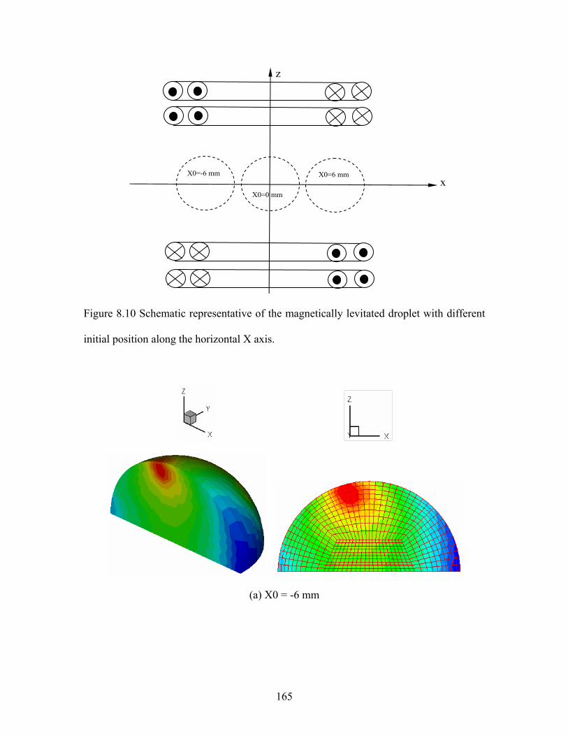
165

Figure 8.10 Schematic representative of the magnetically levitated droplet with different

initial position along the horizontal X axis.

(a) X0 = -6 mm

x

z

X0=-6 mm

X0=0 mm

X0=6 mm

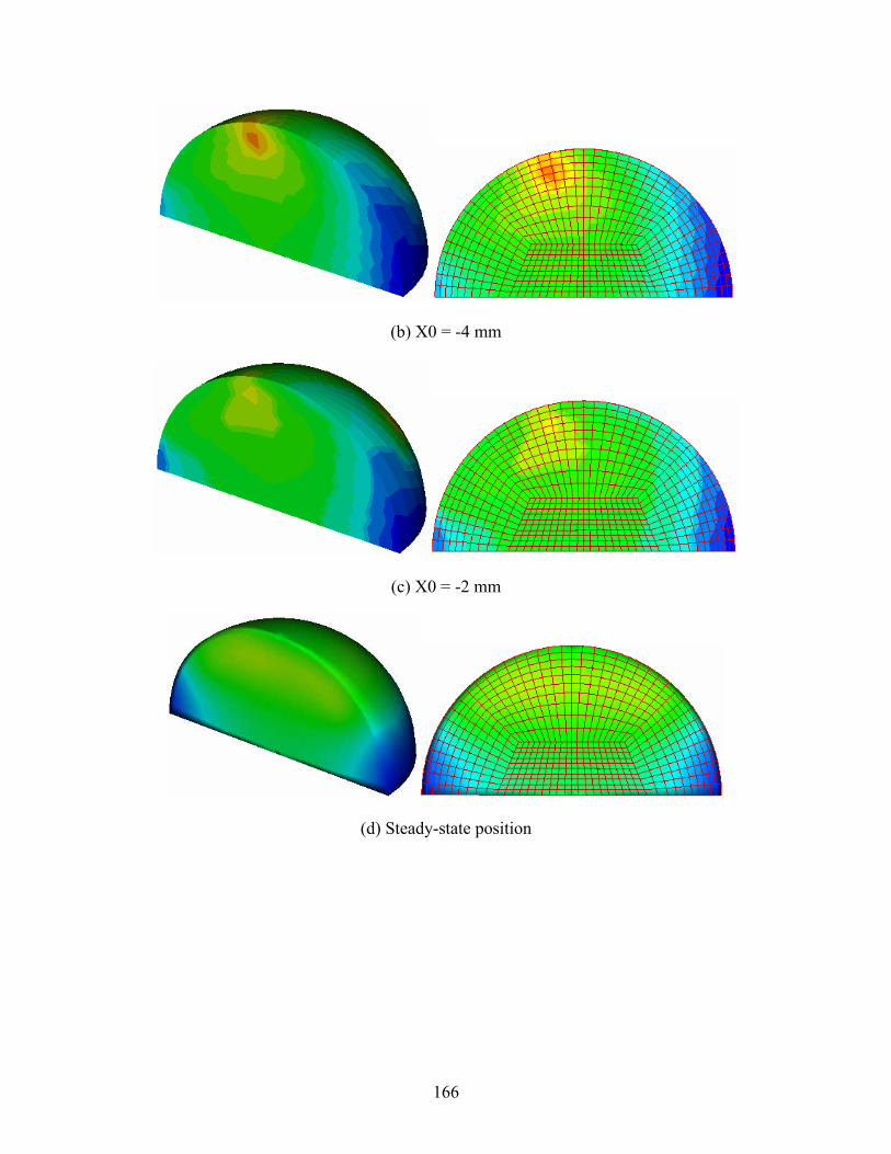
166

(b) X0 = -4 mm

(c) X0 = -2 mm

(d) Steady-state position

167

(e) X0 = 2 mm

(f) X0 = 4 mm

(g) X0 = 6 mm

Figure 8.11 Temperature distribution in a silver droplet induced by positioning coils only

with 1800 out of phase in the TEMPUS system and microgravity conditions with different

initial position along the horizontal X axis.

8.4.3 3-D translation of the magnetically levitated droplet

168

The purpose of this chapter is to study how the magnetically levitated droplet moves. In

this section, we focus on the 3-D translation of the magnetically levitated droplet. The

levitating conducting droplet is assumed to be liquid silver sphere, whose properties are

shown in Table 8.1. In the study of the movement of the magnetically levitated droplet,

the steady-state position of the levitating droplet is assumed to stay at the original point

(0, 0, 0) in the rectangular coordinate. The centers of the coils are fixed above or below

the steady-state position along the z axis. There are no movement and rotation if the

initial position of the magnetically levitated droplet is at the steady-state position.

However, it is difficult to pose the initial position of the magnetically levitated droplet to

the steady-state position. Therefore, it is necessary to investigate the 3-D movement of

the magnetically levitated droplet. Fig. 8.12 (a) presents the 3-D movement of the

magnetically levitated droplet when the initial position vertically deviates from the

steady-state position. Various magnitudes of initial positions (Z0=2 mm, 3 mm) away

from the equilibrium position in the Z-axis are investigated. The computed results (as

seen in Fig. 8.12 (a)) show that the frequency changes a little and it may be assumed to be

kept the same no matter how large deviation from the equilibrium position at the starting

time. Also in Fig. 8.12(a), it is shown that the amplitude of the oscillation along the z-axis

does not change with the time evolving. Like the initial positions away from the

equilibrium position in the vertical direction, the computed results with the initial

positions (X0=2 mm, 3mm) away from the equilibrium position in the horizontal

direction present that the frequencies have small difference for different amplitude of the

oscillation with the evolvement of the time, as shown in Fig. 8.12 (b). Comparing Fig.

169

8.12 (a) with Fig. 8.12 (b) illustrates that the frequency in the vertical movement is

clearly faster than that in the horizontal movement. The computed results show, when the

initial position of the droplet is above 14 mm or below -14 mm along z axis, the

oscillation of the droplet does not occur and the droplet will move away from the

levitated mechanism.

The complex initial deviation from the steady-state position is also investigated.

When the initial position deviate horizontally and vertically from the steady-state position

(0, 0, 0), there is a complex 3-D movement of the magnetically levitated droplet.

Although the 3-D movement is complex, it presents the same rules of variation as the 3-D

movement with only horizontal or vertical deviation when it is projected in the horizontal

X-axis and vertical Z-axis. Fig. 8.13 (a) shows the 3-D movement of the magnetically

levitated droplet with initial position (X0=2 mm, Z0=2 mm), which is projected in the

horizontal X-axis and vertical Z-axis. Fig. 8.13 (b) shows the 3-D movement of the

magnetically levitated droplet with different initial position (X0=3 mm, Z0=3 mm).

Comparison between Fig. 8.12 and Fig. 8.13 depicts that the oscillation of the

magnetically levitated droplet follows the same rules of variation in only horizontal or

vertical directions.

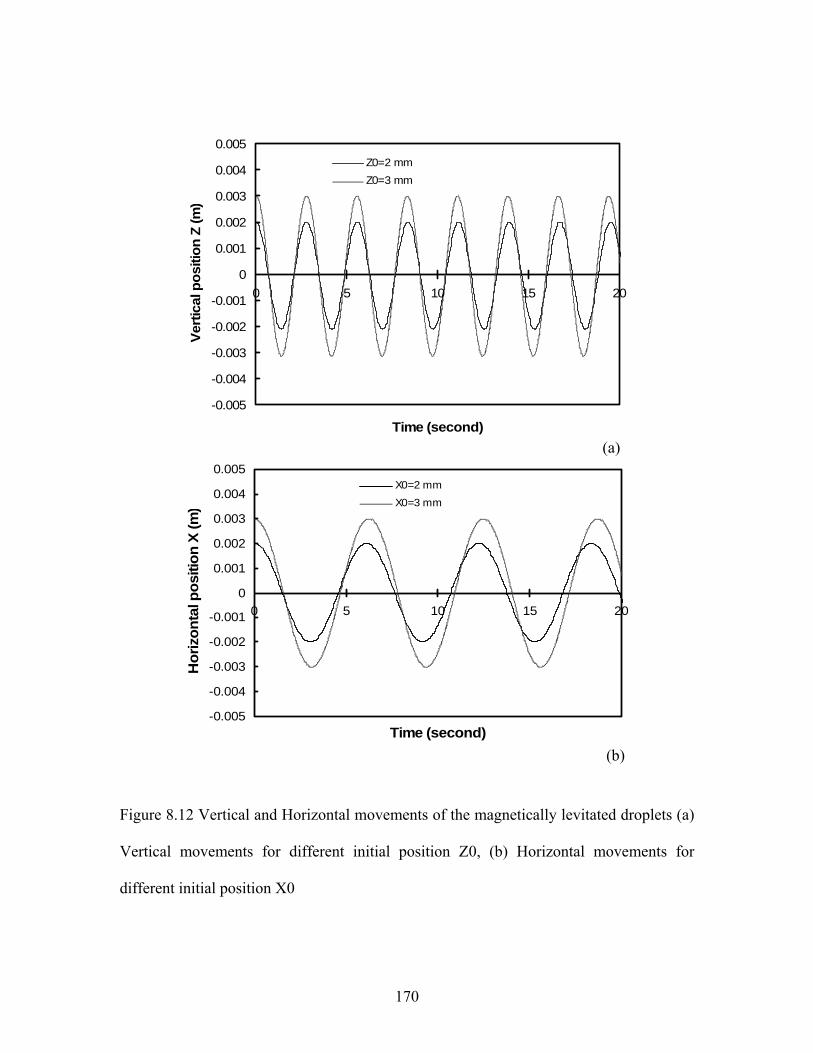
170

-0.005

-0.004

-0.003

-0.002

-0.001

0

0.001

0.002

0.003

0.004

0.005

0 5 10 15 20

Time (second)

Verti

cal p

ositi

on Z

(m)

Z0=2 mmZ0=3 mm

-0.005

-0.004

-0.003

-0.002

-0.001

0

0.001

0.002

0.003

0.004

0.005

0 5 10 15 20

Time (second)

Hor

izon

tal p

ositi

on X

(m)

X0=2 mm

X0=3 mm

Figure 8.12 Vertical and Horizontal movements of the magnetically levitated droplets (a)

Vertical movements for different initial position Z0, (b) Horizontal movements for

different initial position X0

(a)

(b)

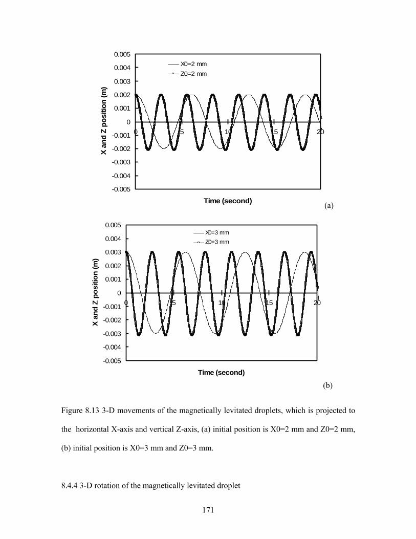
171

-0.005

-0.004

-0.003

-0.002

-0.001

0

0.001

0.002

0.003

0.004

0.005

0 5 10 15 20

Time (second)

X an

d Z

posi

tion

(m)

X0=2 mmZ0=2 mm

-0.005

-0.004

-0.003

-0.002

-0.001

0

0.001

0.002

0.003

0.004

0.005

0 5 10 15 20

Time (second)

X an

d Z

posi

tion

(m)

X0=3 mmZ0=3 mm

Figure 8.13 3-D movements of the magnetically levitated droplets, which is projected to

the horizontal X-axis and vertical Z-axis, (a) initial position is X0=2 mm and Z0=2 mm,

(b) initial position is X0=3 mm and Z0=3 mm.

8.4.4 3-D rotation of the magnetically levitated droplet

(a)

(b)

172

The rotation is another important 3-D movement of the magnetically levitated droplet,

which is emphasized in this section. It has been observed since the early fifties when the

first experiments on the electromagnetic levitation were done that under certain

circumstances the levitated droplet can start to rotate or oscillate which often leads to the

breakdown of the levitation melting. The rotation is undesirable because it can affect the

deformation of the liquid droplet so that the measurement of the thermophysical

properties of the liquid metal becomes not accurate. When the droplet is deformed, it will

further reverse to change the rotation of the liquid droplet. However, in present study, the

droplet is assumed to be solid sphere because the rotation has a little effect on the

spherical solid droplet. Since the droplet is assumed to be spherical and the rotating

movement of the droplet is self-spin-up rotation, the rotation has no effect on the

translation movement of the droplet. Fig. 8.14 (a) shows the variation of the angle

velocity ω with time evolving. Fig. 8.14 (b) shows the rotational angle θ and the vertical

position Z with time evolving. The angle velocities ω with respect to the X and Y axis

presents the oscillation which is similar to sinusoid wave, as shown in Fig. 8.14 (a). In

Fig. 8.14 (b), the rotation angles θ with respect to X and Y axis present the similar

oscillating characteristics to the vertical oscillating movement along the Z axis. However,

the frequency of the oscillation of the rotation angles θ is lower than that for the vertical

oscillating movement. Also the center of the oscillation of the rotation angles θ is not at

the angle zero, which is lager than zero with respect to X axis and smaller than zero with

respect to Y axis.

173

-0.1

-0.08

-0.06

-0.04

-0.02

0

0.02

0.04

0.06

0.08

0.1

0 5 10 15 20 25

angular velocity with respect to X axis

angular velocity with respect to Y axis

(a)

-0.5

-0.4

-0.3

-0.2

-0.1

0

0.1

0.2

0.3

0.4

0.5

0 5 10 15 20 25

-0.002

-0.0015

-0.001

-0.0005

0

0.0005

0.001

0.0015

0.002

rotation angle with respect to X axis

rotation angle with respect to Y axis

vertical position Z

(b)

Figure 8.14 Rotating movement of the magnetically levitated droplet with the initial

position (X0=0, Z0=1 mm), (a) variation of Angular velocity ω with time evolving (b)

variation of rotation angle θ and vertical position Z with time evolving.

Time (second)

Rot

atio

n an

gle θ

(rad

)

Ver

tical

Pos

ition

Z (m

)

Time (second)

Ang

ular

Vel

ocity

ω (r

ad/s

)

174


This chapter presents the numerical study of the 3-D movement of the magnetically

levitated spherical droplet using the coupled boundary and finite element methods. The

hybrid boundary and finite element methods are compared with the various analytical

solutions. The Whitney edge elements are used in both boundary and finite elements,

which avoids the spurious solutions using the node elements. The numerical model is

further tested against with the available results by calculating the Joule heating in the

magnetically levitated droplet surrounded by different coils. The computed results agree

with the results from the other researchers very well. When the 3-D horizontal and

vertical movement of the droplet is computed in the magnetic levitation mechanism, it is

found that the change of the magnitude of the initial position away from the equilibrium

has no effect on the frequency and the amplitude of the oscillation of the droplet

increases with the time evolving. The rotation of the droplet is also investigated. The

variation of the angular velocity and rotational angle with time evolving is depicted.

175

BIBLIOGRAPHY

Adornato, P. M., Brown, R. A., 1983, Shape and stability of electrostatically levitated drops. Proc. R. Soc. London A, 389, pp. 101-117. Ai, X., and Li, B.Q., 2004 Melt flow instability and turbulence in electro-magnetically levitated droplets, Materials and Manufacturing Process, Vol. 19(4), pp.737-759 Ajayi, O.O., 1978, A note on Taylor’s electrohydrodynamic theory, Proc. R. Soc. London A, 364, pp. 499-508 Akarapu, R., Huo, Y., Li, B.Q., Tang, J. and Liu, F., Integrated modeling of microwave food processing and comparison with experimental measurements, Journal of Electromagnetic Power and Microwave Technology, Accepted Bayazitoglu, Y. and Sathuvalli, U.B., 1994, Eddy current heating in an electrically conducting sphere, J. Materials Processing and Manuf. Sci., Vol. 3, pp. 117-141 Bayazitoglu, Y. and Sathuvalli, U.B., 1996a, The Lorentz forces on an electrically conducting sphere in an alternating magnetic field, IEEE Trans. on Magn., Vol. 32(2), pp. 386-400 Bayazitoglu, Y., Sathuvalli, U.B., Suryanarayana, P.V.R. and Mitchell, G.F., 1996b, The Lorentz forces on an electrically conducting sphere in an alternating magnetic field, Physics of Fluids, Vol. 8(2), pp. 370-383 Brazier-Smith, P.R., 1971a, Stability and shape of isolated and pairs of water drops in an electric field, Physics Fluids, 14, pp. 1-6 Brazier-Smith, P.R., Brook, M., Latham, J., Saunders, C.P.R. and Smith, M.H., 1971b, The vibration of electrified water drops. Proc. R. Soc. Lond., A322, pp. 523-534 Brown, R.A. and Scriven, L.E., 1980, The shape and stability of rotating liquid drops, Proc. R. Soc. London A, 371, pp. 331-357 Duff, I.S. and Reid, J.K., 1996, The design of MA48, a code for the direct solution of sparse unsymmetric linear systems of equations, ACM Trans. Math. Softw., 22(2), pp. 187-226 Engelman, M.S., Sani, R.L., Gresho, P.M., 1982 The implementation of normal and tangential velocity boundary conditions in finite element codes for incompressible fluid flow, Int. J. Num. Meth. Fluid, 2, pp. 225-238.

176

Enokizono, M., Todaka, T., Yokoji, K., Wada, Y., Matsumoto, I., 1995, Three-dimensional moving simulation of levitation-melting method, IEEE TRANSACTIONS ON MAGNETICS, Vol. 31 (3), pp. 1869-1872 Feng, J. Q. and Beard, K. V., 1990, Small-Amplitude Oscillations of Electrostatically Levitated Drops. Proc. R. Soc. London A, 430, No. 1878, pp. 133. Flemings, M. C., Trapaga, G. and Hyers, R., 1996, The measurement of the viscosity and surface tension of undercooled melts under microgravity conditions and supporting MHD calculations, NASA Microgravity Materials Science Conference, Huntsville, AL, 76. Huo, Y., Li, B.Q., 2004a, Three-dimensional marangoni convection in electrostatically positioned droplets under microgravity, Int. J. Heat Mass Trans. 47, pp. 3533-3547 Huo, Y., Song, S.P. and Li, B.Q., 2004b, Droplet deformation and 2-D/3-D Marangoni flow phenomena in droplets levitated by electric fields, Materials and Manufacturing Process 19(4), pp. 761-775 Huo, Y., Li, B.Q., and Akarapu, R., 2004c A finite element-boundary integral method for 3-D electromagnetic heating analysis, ASME Heat Transfer/Fluids Engineering Summer Conference, Charlotte, North Carolina Huo, Y. and Li, B.Q., 2005a, A mathematical model for marangoni flow and mass transfer in electrostatically positioned droplets, Metallurgical and Materials Transactions B, Volume 36B, pp. 271-281 Huo, Y. and Li, B.Q., 2005b, Boundary/finite element modeling of 3-d electromagnetic heating during microwave food processing, ASME Journal of Heat Transfer, in print Jackson, J.D., 1975, Classical Electrodynamics (2nd edition), New York: Wiley James R. Melcher, Continuum electromechanics. 1981 Cambridge, Mass.: MIT Press Johns, P.B. and Beurle, R.L., 1971, Numerical solution of two-dimensional scattering problems using a transmission line matrix, Proc. Inst. Eng., Vol. 118, 1203-1208. Johnson, W.L., Schroers, J. and Rhim, W.K., 2002, Studies of properties of undercooled glass forming metallic alloys, Materials Science Conference, Huntsville AL, pp. 307 Li, B.Q., 1993, The magnetothermal phenomena in electromagnetic levitation processes, Int. J. Eng. Sci., Vol. 31, No. 2, pp. 201-220 Li, B.Q., 1994a, The fluid flow aspects of electromagnetic levitation processes, Int. J. Eng. Sci., Vol. 32(1), pp. 45-67

177

Li, B.Q., 1994b, The transient magnetohydrodynamics in electromagnetic levitation processes, Int. J. Eng. Sci., Vol. 32(8), pp. 1315-1336 Li, B.Q., Cui, X. and Song, S.P., A Galerkin boundary element formulation of surface radiation problems, Int. J. Boundary Element Analysis, in print Li, B.Q., Song, S.P., 1999, Thermal and fluid flow aspects of magnetic and electrostatic levitation of liquid droplets, J. Microgravity Sci. Tech., Vol. XI No. 4, pp. 134-143 Lohofer, G., 1989, Theory of an electromagnetically levitated metal sphere I: absorbed power, SIAM J. Appl. Math., Vol. 49 (2), pp. 567-581 Lohofer, G., 1993, Force and torque of an electromagnetically levitated metal sphere, J. Quarterly Appl. Math., LI(3), pp. 495 Lohofer, G., 1994, Magnetization and impedance of an inductively coupled metal sphere, Int. J. Eng. Sci., 32(1), pp. 107 Mestel, A.J., 1982, Magnetic levitation of liquid metals, J. Fluid. Mech., Vol. 117, pp. 17-43 McDonald, B.H., Wexler, A., 1972, Finite element solution of unbounded field problems, IEEE Trans. Microwave Theory Tech., MTT-20, pp. 841-847 Muhlbauer, A., Muiznieks, A. and Jakowitsch, A., 1991, Modeling of the electromagnetic field in induction furnaces with a cold crucible, industrielle Electrowarme, Vol. B3, pp. 130-141 Muck, O., Germ. Pat. No. 422004 (1923) Natarajan, R. and Brown, R.A., 1987, The role of three-dimensional shapes in the break-up of charged drops, Proc. R. Soc. London A, 410, pp. 209-227 Okress, E.C., Wroughton, D.M., Comenetz, G., Brace, P.H., and Kelly, J.C.R., 1952, Electromagnetic levitation of Solid and Molten Metals, J. Appl. Phy., Vol. 23, No. 5, pp. 545-552 Paradis, P.F. and Rhim, W.K., 1999, Thermophysical properties of zirconium at high temperature, J. Mater. Res., Vol. 14 (9), pp.3713 Rayleigh, J.W.S., 1882, On the equilibrium of liquid conducting mass charged with electricity. Phil. Mag., 14, 184. Reitz, J. R., Milford, F. J. and Christy, R. W. 1979, Foundations of electromagnetic theory. Addison-Wesley, Reading, MA.

178

Rhim, W.K., Chung, S.K., Barber, D., Man, K.F., Gutt, G., and Rulison, A., 1993, An electrostatic levitator for high-temperature containerless materials processing in lg, Rev. Sci. Instrum, 64 (10), pp. 2961-2970 Rhim, W.K., 1997a, Private Communication, Jet Propulsion Laboratory, California Institute of Technology, Pasadena, CA. Rhim, W.K., 1997b, Thermophysical property measurements of molten semiconductors, NASA Microgravity Materials Science Conference, Ed. F. Szofran, D. McCauley and C. Walker, 427 Rony, P.B., 1969, The electromagnetic levitation melting of metals, Trans. Vac. Met. Conf., American Vacuum Society, Boston, 55-135 Rosenkilde, C.E., 1969, A dielectric fluid drop in an electric field, Proc. R. Soc. Lond., A312, pp.473-494 Sadhal, S.S., Trinh, E.H. Wagner, P., 1996, Thermocapillary Flows in a Drop With Unsteady Spot Heating in a Microgravity Environment. Journal of Microgravity Sci. Tech., Vol. 9, No. 2, pp. 80 Sathuvalli, U.B. and Bayazitoglu, Y., 1993, Electromagnetic force calculations for a concial coil, Met. Trans., Vol. 24B, pp. 737-748 Sathuvalli, U.B. and Bayazitoglu, Y., 1994, The Lorentz force on a sphere due to an axisymmetric non-homogeneous alternating magnetic field, ASME Winter Meeting, AMD Vol. 194, 293-305 Silvester, P.P., Hsieh, M.S., 1971, Finite element solution of 2-dimensional exterior field problems. IEE Proc., 118, pp. 1743-1747 Song, S.P., Li, B.Q., and Khodadadi, J.M., 1998a, Coupled boundary/finite element solution of magnetothermal problems, Int. J. Num. Meth. Heat and Fluid Flow, 8(3), pp. 321-349 Song, S.P. and Li, B.Q., 1998b, A boundary/finite element analysis of magnetic levitation systems in normal and micro gravity: surface deformation and thermal phenomena, ASME Journal of Heat Transfer, 120, pp. 491-503 Song, S.P., Li, B.Q., 1999a, A coupled boundary/finite element method for the computation of magnetically and electrostatically levitated droplet shapes, Int. J. Numer. Meth. Engng., VOL. 44, pp. 1055-1077 Song, S.P. 1999b, Finite element analysis of surface oscillation, fluid flow, and heat transfer in magnetically and electrostatically levitated droplets, Ph.D thesis, Washington State University, Pullman, WA

179

Song, S.P., Dailey, P., Li, B.Q., 2000a, Effects of heating source arrangements on internal convection in electrostatically levitated droplets. AIAA J. Thermophy. Heat Trans., 14 (3), pp. 335-362. Song, S.P. and Li, B.Q., 2000b, Free surface shapes and thermal convection in electrostatically levitated droplets, Int. J. Heat Mass Trans., 43, pp. 3589-3606. Song, S.P., Li, B.Q., 2001, A hybrid boundary/finite element method for simulating viscous flows and shapes of droplets in electric fields, Int. J. Comp. Fluid Dynamics, 15, pp. 293-308. Suryanarayana, P.V.R. and Bayazitoglu, Y., 1991, Effect of static deformation and external forces on the oscillations of levitated droplets, Physics of Fluids A., Vol. 3, pp. 967-977 Taylor, G.I., 1964, Disintegration of water drops in an electric field, Proc. R. Soc. Lond. A, 280, pp. 383-397 Taylor, G.I., 1966, The force exerted by an electric field on a long cylindrical conductor, Proc. R. Soc. Lond. A, 291, pp. 145-159 Torza, S., Cox, R.G., and Mason, S.G., 1971, Electrohydrodynamics deformation and burst of liquid drops. Phil. Trans. R. Soc. Lond. A. 269, pp. 295 Tsamopoulos, J.A. and Brown, R.A., 1984, Resonant oscillations of inviscid charged drops, J. Fluid Mech., vol. 147, pp. 373-395 Weatherburn, C.E., 1930, Differential geometry of three dimensions. Cambridge University Press Fetter Lane, London Zgraja, J., 1991, The current concentrations for induction heating, industrielle Electrowarme, Vol. B3, pp. 142-148 Zong, J.H., Li, B.Q., and Szekely, J., 1992, The electrodynamic and hydrodynamic phenomena in magnetically-levitated droplets, Part I. steady state behavior, Acta Astronautica, 26(6), pp. 435-449 Zong, J.H., Li, B.Q., and Szekely, J., 1993, The electrodynamic and hydrodynamic phenomena in magnetically-levitated droplets, Part II. transient behavior and heat transfer considerations, Acta Astronautica, 29(4), pp. 305-311

Documents

FINITE ELEMENT MODELING OF INTERNAL FLOW AND …€¦ · The author would like to thank Dr. Gary, ... FINITE ELEMENT MODELING OF INTERNAL FLOW AND STABILITY OF DROPLETS LEVITATED