Embed Size (px)
Citation preview

Old Dominion UniversityODU Digital CommonsMechanical & Aerospace Engineering Theses &Dissertations Mechanical & Aerospace Engineering
Winter 2001
Finite Element Analysis and Active Control forNonlinear Flutter of Composite Panels UnderYawed Supersonic FlowKhaled Abdel-MotagalyOld Dominion University
Follow this and additional works at: https://digitalcommons.odu.edu/mae_etdsPart of the Aerospace Engineering Commons, and the Applied Mechanics Commons
This Dissertation is brought to you for free and open access by the Mechanical & Aerospace Engineering at ODU Digital Commons. It has beenaccepted for inclusion in Mechanical & Aerospace Engineering Theses & Dissertations by an authorized administrator of ODU Digital Commons. Formore information, please contact [email protected].
Recommended CitationAbdel-Motagaly, Khaled. "Finite Element Analysis and Active Control for Nonlinear Flutter of Composite Panels Under YawedSupersonic Flow" (2001). Doctor of Philosophy (PhD), dissertation, Mechanical & Aerospace Engineering, Old DominionUniversity, DOI: 10.25777/1fvd-ra53https://digitalcommons.odu.edu/mae_etds/210

FINITE ELEMENT ANALYSIS AND ACTIVE CONTROL
FOR NONLINEAR FLUTTER OF COMPOSITE PANELS
UNDER YAWED SUPERSONIC FLOW
Khaled Abdel-MotagalyB.S. July 1991, Cairo University, Egypt M.S. July 1995, Cairo University, Egypt
A Dissertation Submitted to the Faculty of Old Dominion University in Partial Fulfillment of the
Requirement for the Degree of
DOCTOR OF PHILOSOPHY
AEROSPACE ENGINEERING
OLD DOMINION UNIVERSITY December 2001
by
Approved by :
Chuh Mei (Director)
Osama Kandil (Member)
Jen-K.uang Huang (Member)
Donald Kunz (Member^
Reproduced with permission of the copyright owner. Further reproduction prohibited without permission.

ABSTRACT
FINITE ELEMENT ANALYSIS AND ACTIVE CONTROL FOR NONLINEAR FLUTTER OF COMPOSITE PANELS
UNDER YAWED SUPERSONIC FLOW
Khaled Abdel-Motagaly Old Dominion University, 2001
Director: Dr. Chuh Mei
A coupled structural-electrical modal finite element formulation for composite
panels with integrated piezoelectric sensors and actuators is presented for nonlinear panel
flutter suppression under yawed supersonic flow. The first-order shear deformation
theory for laminated composite plates, the von Karman nonlinear strain-displacement
relations for large deflection response, the linear piezoelectricity constitutive relations,
and the first-order piston theory of aerodynamics are employed. Nonlinear equations of
motion are derived using the three-node triangular MIN3 plate element. Additional
electrical degrees o f freedom are introduced to model piezoelectric sensors and actuators.
The system equations o f motion are transformed and reduced to a set of nonlinear
equations in modal coordinates. Modal participation is defined and used to determine the
number of modes required for accurate solution.
Analysis results for the effect of arbitrary flow yaw angle on nonlinear supersonic
panel flutter for isotropic and composite panels are presented. The results show that the
flow yaw angle has a major effect on the panel limit-cycle oscillation amplitude and
deflection shape. The effect of combined aerodynamic and acoustic pressure loading on
the nonlinear dynamic response of isotropic and composite panels is also presented. It is
found that combined acoustic and aerodynamic loads have to be considered for high
aerodynamic pressure values.
Simulation studies for nonlinear panel flutter suppression using piezoelectric self
sensing actuators under yawed supersonic flow are presented for isotropic and composite
panels. Different control strategies are considered including linear quadratic Gaussian
(LQG), linear quadratic regulator (LQR) combined with the extended Kalman filter
(EKF), and optimal output feedback. Closed loop criteria based on the norm of feedback
Reproduced with permission of the copyright owner. Further reproduction prohibited without permission.

control gain (NFCG) and on the norm o f Kalman filter estimator gain (NKFEG) are used
to determine the optimal location of piezoelectric actuators and sensors, respectively.
Optimal sensor and actuator locations for a range of yaw angles are determined by
grouping the optimal locations for different angles within the range. The results
demonstrate the effectiveness o f piezoelectric materials and of the nonlinear output
controller comprised o f LQR state feedback and EKF nonlinear state estimator in
suppressing nonlinear flutter o f isotropic and composite panels at different flow yaw
angles.
Reproduced with permission of the copyright owner. Further reproduction prohibited without permission.

ACKNOWLEDGMENTS
I would like to express my sincere thanks and deepest appreciation to Professor
Chuh Mei for his everlasting assistance, encouragement, support, and patience. His
guidance, inspiring ideas, and enlightening discussion played a key role in the production
of this work. I would also like to extend my sincere thanks and deep gratitude to the other
members o f my dissertation committee: Professors Osama Kandil, Donald Kunz, and
Jen-Kuang Huang. Their invaluable comments and advice are much appreciated and are
an added value to this dissertation. I gratefully acknowledge the financial support of the
Aerospace Engineering Department during the course of my research.
I extend my thanks and gratitude to Professor Sayed Dessoki, who taught me a lot
during my entire career. Last, but not least, special acknowledgment and thanks go to my
parents and my wife for their everlasting love and encouragement. Without their support,
this work would have been impossible.
Reproduced with permission of the copyright owner. Further reproduction prohibited without permission.

TABLE OF CONTENTS
Page
LIST OF TA B LE S.......................................................................................................................viii
LIST OF FIG U RES....................................................................................................................... ix
LIST OF SY M BO LS....................................................................................................................xiv
Chapter
I. INTRODUCTION AND LITERATURE SU R V EY ...................................................... 1
1.1 Introduction.................................................................................................................. 1
1.2 Background and Literature S u rv ey ........................................................................... 2
1.2.1 Panel F lu tte r .....................................................................................................2
1.2.2 Piezoelectric Sensors and A ctuators.............................................................8
1.2.3 Panel Flutter Suppression Using Piezoelectric M aterials..................... 11
1.3 Outline of the S tu d y ................................................................................................ 13
II. FINITE ELEMENT FO RM U LATIO N........................................................................ 19
2.1 Introduction..................................................................................................................19
2.2 Element Displacement Functions........................................................................... 20
2.3 Nonlinear Strain-Displacement R elations............................................................ 22
2.4 Electrical Field-Potential R elations........................................................................23
2.5 Linear Piezoelectricity Coupling E quations.........................................................24
2.6 Constitutive E quations..............................................................................................25
2.7 Laminate Resultant Forces and M om ents.............................................................26
2.8 Aerodynamic Pressure L oading ..............................................................................27
2.9 Element Equations o f Motion and M atrices.........................................................28
2.9.1 Generalized Hamilton’s P rincip le ............................................................ 28
2.9.2 Element Stiffness and Electromechanical Coupling M atrices...........29
2.9.3 Element Mass M atrices..............................................................................34
2.9.4 Element Aerodynamic M atrices .............................................................. 35
2.9.5 Element Equations of M o tio n .................................................................. 36
2.10 System Equations of M otion ...................................................................................37
2.11 Piezoelectric Actuator and Sensor E quations......................................................38
Reproduced with permission of the copyright owner. Further reproduction prohibited without permission.

2.11.1 Piezoelectric Material as Actuators and S enso rs .................................. 38
2.11.2 Piezoelectric Material as Self-Sensing A ctuators.................................40
III. MODAL REDUCTION AND SOLUTION PRO CED U RE.......................................45
3.1 Introduction..................................................................................................................45
3.2 Governing Equations................................................................................................. 46
3.3 Modal Transformation and R eduction................................................................... 48
3.4 Solution Procedure..................................................................................................... 51
3.4.1 Time Domain M eth o d ................................................................................51
3.4.2 Frequency Domain M ethod .......................................................................51
3.4.2.1 Critical Flutter B oundary.......................................................... 51
3.4.2.2 Nonlinear Flutter Limit-Cycle O scilla tion ............................ 53
IV. FINITE ELEMENT ANALYSIS R ESU LTS................................................................57
4.1 Introduction................................................................................................................. 57
4.2 Finite Element V alidation.........................................................................................57
4.2.1 Natural Frequencies....................................................................................57
4.2.2 Piezoelectric Static A ctuation .................................................................. 58
4.2.3 Linear and Nonlinear F lu tte r.................................................................... 58
4.2.4 Nonlinear Random R esponse................................................................... 59
4.3 Effect o f Flow Yaw angle on Nonlinear Panel F lu tte r........................................ 60
4.3.1 Isotropic P anels........................................................................................... 60
4.3.2 Composite P an e ls ....................................................................................... 61
4.3.3 Triangular P an e l..........................................................................................62
4.4 Effect of Combined Supersonic Flow and Acoustic Pressure L oad ing 62
4.4.1 Random Surface P ressu re .........................................................................62
4.4.2 Isotropic P an e l.............................................................................................63
4.4.3 Composite P an e l.........................................................................................64
4.5 Sum m ary..................................................................................................................... 65
V. CONTROL METHODS AND OPTIMAL PLACEMENT
OF PIEZOELECTRIC SENSORS AND A C TA U TO RS........................................... 99
5.1 Introduction................................................................................................................ 99
5.2 State Space Representation..................................................................................... 99
Reproduced with permission of the copyright owner. Further reproduction prohibited without permission.

5.3 Control M ethods................................................................................................... 101
5.3.1 Linear Quadratic Regulator (L Q R )...................................................... 101
5.3.2 Optimal Linear State Estim ation.......................................................... 102
5.3.3 Linear Quadratic Gaussian Controller (L Q G )................................... 103
5.3.4 Extended Kalman Filter (E K F )............................................................ 104
5.3.5 Nonlinear Controller using EKF and L Q R ........................................ 104
5.3.6 Optimal Output Feedback..................................................................... 105
5.4 Optimal Placement of Piezoelectric Sensors and A ctuators......................... 105
VI. NONLINEAR PANEL FLUTTER SUPPRESSION R E SU LT S.......................... 109
6.1 Introduction............................................................................................................ 109
6.2 Square Isotropic P anel......................................................................................... 109
6.2.1 Optimal Placement of Self-Sensing Piezoelectric A ctuators......... 110
6.2.2 Controller S tudy ...................................................................................... I l l
6.2.2.1 LQR C ontroller....................................................................... 112
6.2.2.2 LQG C ontroller....................................................................... 113
6.2.2.3 Nonlinear Output Controller (EK F+LQ R )......................... 113
6.2.2.4 Optimal Output Feedback C ontro ller.................................. 114
6.2.2.5 Controller Robustness............................................................ 115
6.2.3 Panel Flutter Control with Yawed F lo w ............................................ 116
6.3 Composite P an e l................................................................................................. 118
6.4 Triangular P an e l................................................................................................. 119
6.5 S um m ary............................................................................................................. 120
VII. SUMMARY AND CONCLUSIONS......................................................................... 158
R EFER EN C ES........................................................................................................................... 161
APPENDCIES ............................................................................................................................ 172
A. MIN3 ELEMENT STRAIN INTERPOLATION M A TR IC ES............................ 172
B. COORDINATE TRANSFORM ATION.................................................................... 174
B .l Transformation of Lamina Stiffness M atrices................................................. 174
B.2 Transformation of Piezoelectric C onstants....................................................... 175
C. SOLUTION PROCEDURE FOR OPTIMAL OUTPUT FEED BA CK .............. 176
V IT A ............................................................................................................................................. 177
Reproduced with permission of the copyright owner. Further reproduction prohibited without permission.

LIST OF TABLES
Table Page
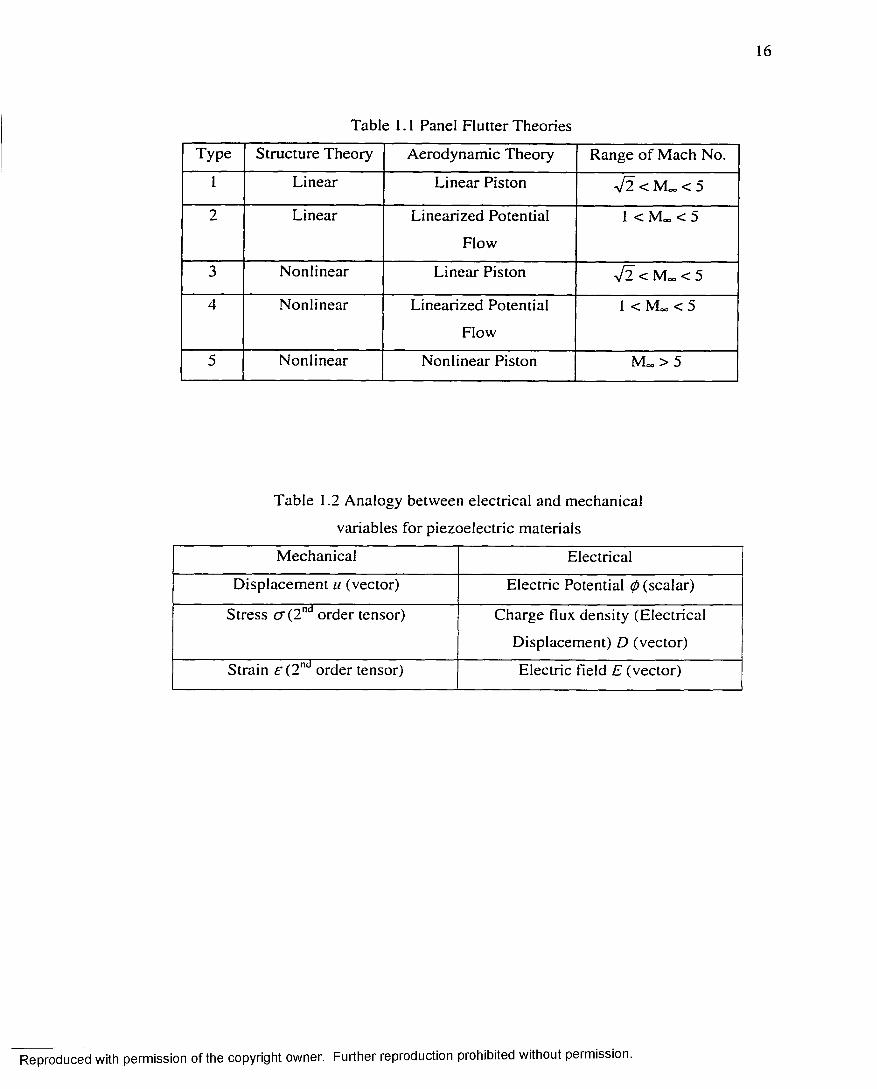
1.1 Panel Flutter T heories ................................................................................................... 16
1.2 Analogy between electrical and mechanical variables
for piezoelectric m ateria ls............................................................................................. 16
4.1 Material properties for the different materials used for
Finite element validation and analysis resu lts ............................................................. 66
4.2 Comparison between natural frequencies using MIN3 element
and using analytical solution for square isotropic p an e l........................................... 67
4.3 Comparison of static deflection for the piezoelectric bimorph
beam (10'7 m) using different m ethods........................................................................ 67
4.4 Comparison of nondimensional linear flutter boundary using
different methods at different flow an g les ...................................................................68
4.5 Comparison of the RMS (Wmax/h) for a simply supported rectangular
(15x12x0.04 in.) isotropic plate under acoustic pressure loading only
using different methods and mode num bers................................................................68
4.6 Modal participation values at various limit-cycle amplitudes and different
flow angles for simply supported square p an el........................................................... 69
4.7 Modal participation values at various limit-cycle amplitudes and different flow
angles for simply supported rectangular graphite/epoxy [0/45/-45/90]s panel ... 70
4.8 Modal participation values at various limit-cycle amplitudes and different flow
angles for simply supported rectangular graphite/epoxy [-40/40/-40] p an e l 71
4.9 Modal convergence for clamped rectangular [0/45/-45/90]s graphite/epoxy
panel at SPL = 120 dB and X = 800 ............................................................................. 72
4.10 Modal participation for a clamped rectangular [0/45/-45/90]s graphite/epoxy
panel at SPL = 120 dB and X = 800 .............................................................................. 72
6.1 Mechanical and electrical properties for PZT5A piezoelectric ceram ics 122
6.2 Comparison of different controllers performance for nonlinear
panel flutter suppression.............................................................................................. 122
Reproduced with permission of the copyright owner. Further reproduction prohibited without permission.
LIST OF FIGURES
Figure Page
1.1 Explanation of nonlinear panel flutter phenom enon................................................. 17
1.2 Schematic of traditional isotropic piezoelectric elem ent.......................................... 18
2.1 Composite panel under yawed supersonic flow and acoustic
pressure loading ................................................................................................................ 42
2.2 Composite laminate composed of n layers with n p piezoelectric lay e rs .................43
2.3 MIN3 element geometry and area coordinates............................................................44
3.1 Configuration of self-sensing piezoelectric actuators for bending moment
actuation and transverse displacement sen sin g ..........................................................55
3.2 Iterative solution procedure for nonlinear panel flutter limit-cycle resp o n se 56
4.1 Typical MIN3 elements mesh used to model rectangular and
triangular panels.................................................................................................................73
4.2 Clamped piezoelectric bimorph beam modeled using MIN3 elem ents..................74
4.3 Validation of flutter limit-cycle amplitude for simply supported square
isotropic p a n e l.................................................................................................................... 75
4.4 Validation of flutter limit-cycle amplitude for simply supported square
[0/45/-45/90]s lam inate.....................................................................................................76
4.5 Finite element mesh convergence for simply supported isotropic square
panel at 45° flow angle and using 16 m o d es ................................................................ 77
4.6 Modal convergence for simply supported isotropic
square panel at 0° flow a n g le .......................................................................................... 78
4.7 Modal convergence for simply supported isotropic
square panel at 45° flow a n g le ........................................................................................ 79
4.8 Effect of flow yaw angle on limit-cycle amplitude for
simply supported isotropic square p a n e l....................................................................... 80
4.9 Effect o f panel aspect ratio at different yaw angles on limit-cycle
amplitude for simply supported isotropic p a n e ls ........................................................81
4.10 Flutter mode shape at different flow angles for simply supported
isotropic square p an e l.......................................................................................................82
Reproduced with permission of the copyright owner. Further reproduction prohibited without permission.

X
4 .1 1 Modal convergence for simply supported rectangular graphite/epoxy
[0/45/-45/90]s panel at 45° flow a n g le .......................................................................... 83
4.12 Effect of flow yaw angle on limit-cycle amplitude for simply
supported rectangular graphite/epoxy [0/45/-45/90]s p a n e l.....................................84
4.13 Flutter mode shape at different flow angles for simply supported
rectangular graphite/epoxy [0/45/-45/90]s p a n e l........................................................ 85
4.14 Modal convergence for simply supported rectangular graphite/epoxy
[-40/40/-40] panel at 45° flow a n g le ..............................................................................86
4.15 Effect of flow yaw angle on limit-cycle amplitude for simply
supported rectangular graphite/epoxy [-40/40/-40] p a n e l......................................... 87
4.16 Flutter mode shape at different flow angles for simply supported rectangular
graphite/epoxy [40/-40/40] p an e l....................................................................................88
4.17 Modal convergence for simply supported triangular isotropic panel
at 45° flow a n g le ................................................................................................................89
4.18 Effect o f flow yaw angle on limit-cycle amplitude for simply supported
triangular isotropic p an e l................................................................................................. 90
4.19 Power spectral density of random input pressure at SPL = 9 0 d B .......................... 91
4.20 RMS of maximum deflection for simply supported square isotropic panel
under combined acoustic and aerodynamic pressu res...............................................92
4.21 Time and frequency response for simply supported square isotropic panel
at SPL = 100 dB and X = 0 ...............................................................................................93
4.22 Time and frequency response for simply supported square
isotropic panel at SPL = 120 dB and X = 0 .................................................................. 94
4.23 Time and frequency response for simply supported square
isotropic panel at SPL = 0 dB and X = 800 ......................................................... 95
4.24 Time and frequency response for simply supported square
isotropic panel at SPL = 100 dB and X = 800 .................................................... 96
4.25 Time and frequency response for simply supported square
isotropic panel at SPL = 120 dB and X = 800 .................................................... 97
4.26 RMS of maximum deflection for clamped rectangular
graphite/epoxy [0/45/-45/90]s p a n e l.............................................................................98
Reproduced with permission of the copyright owner. Further reproduction prohibited without permission.

5.1 Block diagram representation of the LQG contro ller............................................ 107
5.2 Nonlinear dynamic compensator for nonlinear panel flutter
suppression using EKF and L Q R ............................................................................... 108
6.1 Contours o f (a) NFCG and (b) NKFEG for simply supported square
isotropic panel at 0° flow an g le .................................................................................. 123
6.2 Contours o f (a) NFCG and (b) NKFEG for simply supported square
isotropic panel at 45° flow an g le ................................................................................ 124
6.3 Selected self-sensing piezoelectric actuators placement and size for optimal
actuation and optimal sensing on square isotropic panel at 0° flow an g le 125
6.4 Self-sensing piezoelectric actuators placement and size for optimal
actuation and optimal sensing on square isotropic panel at 45° flow an g le 126
6.5 Variation of first 4 linear modes versus X for isotropic panel with
and without added piezoelectric m aterial................................................................ 127
6.6 Open loop poles for isotropic square panels with embedded piezoelectric
material at different values of nondimensional dynamic p ressu re ....................... 128
6.7 Limit-cycle amplitude and control inputs time history for square isotropic
panel using LQR control at X = 1500 ........................................................................ 129
6.8 Comparison between actual LCO amplitude and estimated LCO amplitude
using Kalman filter at X = 1000 ................................................................................. 130
6.9 Comparison between actual LCO amplitude and estimated LCO amplitude
using Kalman filter at X = 2000 ................................................................................. 131
6.10 Performance of LQG controller at X = 1500 ........................................................... 132
6 .11 Performance of LQG controller at the maximum suppressible
dynamic pressure, Amax = 920 .................................................................................. 133
6.12 Comparison between actual and estimated LCO amplitude
using extended Kalman filter at X = 2000 ................................................................ 134
6.13 Performance of LQR+EKF nonlinear output compensator at X = 1500 ............ 135
6.14 Performance of LQR+EKF nonlinear output controller at X = 1500 with
(a) -25% and (b) +25% uncertainty in the model nonlinear stiffness matrix .... 136
6.15 Performance of optimal output feedback controller using two
self-sensing actuators at Amax = 1000 ...................................................................... 137
Reproduced with permission of the copyright owner. Further reproduction prohibited without permission.

6.16 Performance of optimal output feedback controller using single leading edge
actuator and two displacement sensors at Amax = 11 0 0 ........................................ 138
6.17 Effect of +25% mismatch in A between design model and simulation model
on LQR and LQR+EKF control performance at A = 1200 .................................... 139
6.18 Effect of design model linear stiffness variation on The LQR+EKF
controller performance at A = 1 5 0 0 ........................................................................... 140
6.19 Effect of design model linear stiffness variation on optimal output
feedback controller performance at A = 1100.......................................................... 141
6.20 Performance of EKF+LQR controller designed for zero flow angle
at A = 800 and 45 deg flow a n g le ................................................................................ 142
6.21 Optimal actuator and sensor placement at different flow angles
from 0 to 90° for square isotropic p a n e l..................................................................... 143
6.22 Placement of four self-sensing piezoelectric actuators for optimal
actuation and optimal sensing over the range of [0, 90°] flow
angle for square isotropic p a n e l.................................................................................. 144
6.23 Comparison of panel flutter suppression performance using LQR+EKF
control at different flow yaw angles and using different piezoelectric
placement configurations for a square isotropic p a n e l.......................................... 145
6.24 Performance of LQR+EKF controller for square isotropic panel with 4
self-sensing piezoelectric actuators at 0° flow yaw angle and A = 1500 ........... 146
6.25 Performance of LQR+EKF controller for square isotropic panel with 4
self-sensing piezoelectric actuators at 45° flow yaw angle and A = 1500 ......... 147
6.26 Performance of LQR+EKF controller for square isotropic panel with 4
self-sensing piezoelectric actuators at 90° flow yaw angle and A = 1500 ......... 148
6.27 Optimal actuator placement at different flow angles for [0/45/-45/90]s
composite rectangular p a n e l ........................................................................................ 149
6.28 Optimal placement of 2 embedded piezoelectric actuators that cover flow
angles from 0° to 90° for [0/45/-45/90]s composite rectangular p a n e l................150
6.29 Comparison of panel flutter suppression performance using LQR+EKF
control at different flow yaw angles and using different piezoelectric
actuator configurations for [0/45/-45/90]s rectangular composite p a n e l 151
Reproduced with permission of the copyright owner. Further reproduction prohibited without permission.
Xlll
6.30 Performance o f LQR+EKF controller for rectangular composite panel
at 0° flow yaw angle and X = 900 ............................................................................... 152
6.31 Performance o f LQR+EKF controller for rectangular composite panel
at 45° flow yaw angle and X = 900 ............................................................................ 153
6.32 Performance of LQR+EKF controller for rectangular composite panel
at 90° flow yaw angle and X = 900 ............................................................................ 154
6.33 Optimal actuator placement at different flow angles
for clamped triangular isotropic p a n e l....................................................................... 155
6.34 Optimal placement o f a single self-sensing piezoelectric actuator that
approximately cover all angles from 90° to 180° for
triangular clamped isotropic p an e l.............................................................................. 156
6.35 Performance of the LQR+EKF controller in suppressing nonlinear
panel flutter using different piezoelectric actuator configurations
for the clamped triangular isotropic p a n e l................................................................ 157
Reproduced with permission of the copyright owner. Further reproduction prohibited without permission.

1
CHAPTER I
INTRODUCTION AND LITERATURE SURVEY
1.1 Introduction
Recently, there has been a renewed interest in flight vehicles that operate at high
supersonic and hypersonic Mach numbers, such as the X-38 Crew Return Vehicle
spacecraft for the International Space Station, the X-33 Advanced Technology
Demonstrator, the X-34 Reusable Technology Demonstrator for a launch vehicle, and the
recent NASA Space Launch Initiative (SLI) project. The exterior panels of such vehicles
will be affected by supersonic panel flutter phenomena. These flight vehicles will usually
operate for a range of flow yaw angles and will also be subjected to additional loading
due to random pressure fluctuations (sonic fatigue). This brings an urgent need for panel
flutter analysis at supersonic speeds considering the effect of flow yaw angle and the
effect of additional acoustic loading.
The requirements of energy-efficient, high-strength, and minimum-weight
vehicles have generated an interest in advanced lightweight composite materials. In
addition, higher performance can be obtained by using the recently developed smart or
adaptive materials such as piezoelectric ceramics that are embedded into the laminated
composite panels to control and suppress undesired panel vibrations.
The primary objectives of this study are: (1) to develop a finite element tool for
analyzing nonlinear supersonic flutter of composite panels considering the effects of flow
yaw angle and the effect of additional acoustic loading and (2) to design practical control
methodologies that suppress nonlinear supersonic panel flutter o f composite and isotropic
panels using piezoelectric sensors and actuators considering the effect of flow yaw angle.
The next sections present an overview and literature survey for the main topics of this
research including classical and finite element analysis methods for nonlinear panel
flutter, piezoelectric sensors and actuators, and panel flutter suppression using
piezoelectric materials. An outline of the dissertation is then given at the end of the
chapter.
The journal model used for this dissertation is the AlAA Journal.
Reproduced with permission of the copyright owner. Further reproduction prohibited without permission.

1.2 Background and Literature Survey1.2.1 Panel Flutter
Supersonic panel flutter is a self-excited oscillation of panels exposed to
aerodynamic flow with high Mach numbers. Figure 1.1 shows four different schematics
explaining the panel flutter phenomenon. For dynamic pressures, q , less than the flutter
boundary, random pressure fluctuations due to turbulent boundary layer control the panel
response. At this regime, the panel response can be determined using standard linear
sonic fatigue (noise) analysis techniques and is usually in the small displacement region,
i.e., maximum panel displacement divided by panel thickness { W m io / h ) is much less than
one. As the dynamic pressure increases, the panel stiffness is modified by the
aerodynamic loading such that the first mode natural frequency, co, increases while thd*
second mode natural frequency decreases. At the flutter boundary, the two modes
coalesce and the panel motion becomes unstable, based on linear structure theory.
However, due to the structural nonlinearities (inplane stretching forces) and unlike the
catastrophic failure for wing flutter, the panel motion is limited to a constant amplitude
oscillation. The inplane stretching forces tend to restrain the panel motion so that
bounded limit-cycle oscillations (LCO) are observed as shown in Figure 1.1. The
amplitude of the LCO grows as the dynamic pressure increases. The existence of LCO
implies that large deflection nonlinear structural theory should be used beyond the flutter
critical dynamic pressure to estimate panel response and fatigue life. The flutter LCO
deflection shape depends on many factors such as flow yaw angle, panel boundary
conditions, and composite laminate stacking. An example of flutter deflection shape for
an isotropic simply supported square panel is shown in Figure 1.1.
Since the late fifties and early sixties, there have been many articles in the
literature addressing linear and nonlinear panel flutter. An excellent review article for
linear and nonlinear panel flutter theories and analysis through 1970 is given by Dowell
[1]. Recently, Mei et al. [2], have produced an extensive review of various analytical and
experimental results for nonlinear supersonic and hypersonic panel flutter up to 1999.
Dowell [1] has grouped the vast amount of theoretical literature on panel flutter into four
categories based on the structural and aerodynamic theories used. Gray and Mei [3]
Reproduced with permission of the copyright owner. Further reproduction prohibited without permission.

3
added a fifth category for hypersonic flow. The five different categories o f linear and
nonlinear panel flutter are shown in Table 1.1. The weakness and remedies for the first
four types o f analysis were discussed in detail by Dowell. A review of the finite element
method of type-1 panel flutter analysis was given by Bismark-Nasr [4], A survey on
various analytical methods, including finite element method for nonlinear supersonic
panel flutter type-3 analysis, was given by Zhou et al. [5]. The fundamental theories and
physical understanding of panel flutter are given in detail in published books, [6] and [7],
This study is concerned with the type-3 panel flutter analysis that uses nonlinear structure
theory and linear piston theory of aerodynamics with yawed supersonic flow.
As disclosed by these survey papers, a vast quantity of literature exists on panel
flutter using different aerodynamic theories. The aerodynamic theory employed for the
most part of panel flutter at high supersonic Mach numbers (M„ > 1.6) is the quasi-steady
first order piston theory developed by Ashley and Zartarian [8], If aerodynamic damping
is neglected, the quasi-steady piston theory simplifies to the quasi-static Ackeret theory.
The piston theory, although several decades old, has generally been employed to
approximate the aerodynamic loads on the panel from local pressures generated by the
body’s motion as related to the local normal component of the fluid velocity and the local
pressure. For supersonic Mach numbers, the quasi-steady aerodynamic theory reasonably
estimates the aerodynamic pressures and shows fair agreement between theory and
experiment for plates exposed to static pressure loads and buckled by uniform thermal
expansion, as was shown by Ventres and Dowell [9]. For airflow with Mach numbers
close to one, the full-linearized inviscid potential theory of aerodynamics is usually
employed [10]. For hypersonic panel flutter, the nonlinear unsteady third-order piston
theory is used to develop the aerodynamic pressure, [11] and [3].
The partial nonlinear behavior of a fluttering panel was first considered by several
investigators such as [12-14], They were primarily concerned with determining stability
boundaries o f two-dimensional plates. For nonlinear limit-cycle behavior, a variety of
methods have been employed to assess the panel flutter problem. Galerkin’s method was
used to reduce the governing partial differential equations to a set of coupled ordinary
differential equations in time, which were numerically integrated using arbitrary initial
conditions. The integration was continued until a limit-cycle oscillation of constant
Reproduced with permission of the copyright owner. Further reproduction prohibited without permission.
4
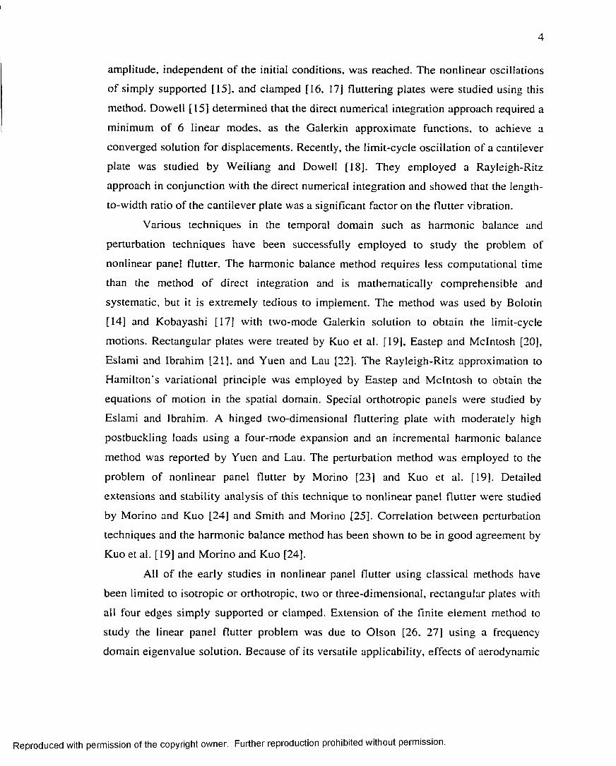
amplitude, independent of the initial conditions, was reached. The nonlinear oscillations
of simply supported [15], and clamped [16, 17] fluttering plates were studied using this
method. Dowell [15] determined that the direct numerical integration approach required a
minimum of 6 linear modes, as the Galerkin approximate functions, to achieve a
converged solution for displacements. Recently, the limit-cycle oscillation of a cantilever
plate was studied by Weiliang and Dowell [18]. They employed a Rayleigh-Ritz
approach in conjunction with the direct numerical integration and showed that the length-
to-width ratio of the cantilever plate was a significant factor on the flutter vibration.
Various techniques in the temporal domain such as harmonic balance and
perturbation techniques have been successfully employed to study the problem of
nonlinear panel flutter. The harmonic balance method requires less computational time
than the method o f direct integration and is mathematically comprehensible and
systematic, but it is extremely tedious to implement. The method was used by Bolotin
[14] and Kobayashi [17] with two-mode Galerkin solution to obtain the limit-cycle
motions. Rectangular plates were treated by Kuo et al. [19], Eastep and McIntosh [20],
Eslami and Ibrahim [21], and Yuen and Lau [22]. The Rayleigh-Ritz approximation to
Hamilton’s variational principle was employed by Eastep and McIntosh to obtain the
equations of motion in the spatial domain. Special orthotropic panels were studied by
Eslami and Ibrahim. A hinged two-dimensional fluttering plate with moderately high
postbuckling loads using a four-mode expansion and an incremental harmonic balance
method was reported by Yuen and Lau. The perturbation method was employed to the
problem of nonlinear panel flutter by Morino [23] and Kuo et al. [19], Detailed
extensions and stability analysis of this technique to nonlinear panel flutter were studied
by Morino and Kuo [24] and Smith and Morino [25]. Correlation between perturbation
techniques and the harmonic balance method has been shown to be in good agreement by
Kuo et al. [19] and Morino and Kuo [24].
All of the early studies in nonlinear panel flutter using classical methods have
been limited to isotropic or orthotropic, two or three-dimensional, rectangular plates with
all four edges simply supported or clamped. Extension of the finite element method to
study the linear panel flutter problem was due to Olson [26, 27] using a frequency
domain eigenvalue solution. Because of its versatile applicability, effects of aerodynamic
Reproduced with permission of the copyright owner. Further reproduction prohibited without permission.

5
damping, complex panel configurations and support conditions, laminated composite
anisotropic panel properties, flow angularities, inplane stresses, and thermal loads can be
easily and conveniently included in the finite element formulation. A survey on the finite
element methods for linear panel flutter was given by Yang and Sung [28] and Bismark-
Nasr [4], and for nonlinear panel flutter by Zhou et al. [5]. Application of the finite
element method to study the supersonic limit-cycle oscillations of two-dimensional
panels was given by Mei [29] using an iterative frequency domain solution. Mei and
Rogers [30] implemented the two-dimensional panel flutter analysis into NASTRAN.
Rao and Rao [31] investigated the supersonic flutter of two-dimensional panels with ends
restrained elastically against rotation. Sarma and Varadan [32] studied the nonlinear
behavior of two-dimensional panels using two solution procedures, both in the frequency
domain. Further extension of the finite element method to treat supersonic limit-cycle
oscillations o f three-dimensional rectangular plates was given by Mei and Weidman [33],
The effects of damping, aspect ratio, inplane forces, and boundary conditions were
considered. Mei and Wang [34] employed an 18-degree of freedom (DOF) triangular
plate bending element to study supersonic limit-cycle behavior of three-dimensional
triangular plates. Han and Yang [35] used the 54-DOF high order triangular plate element
to study nonlinear panel flutter of three-dimensional rectangular plates with inplane
forces.
Few papers in the literature have investigated supersonic limit-cycle oscillations
o f composite panels. Dixon and Mei [36] studied the nonlinear flutter of rectangular
composite panels. The limit-cycle response was obtained using a 24-DOF rectangular
plate element and a linearized updated mode with nonlinear time function (LUM/NTF)
approximate solution procedure. The LUM/NTF solution procedure in the frequency
domain was developed by Gray [11]. Because of the renewed interest in panel flutter at
high-supersonic/hypersonic speeds [37], Gray et al. [3] and [11] extended the finite
element method to investigate the hypersonic limit-cycle oscillations of composite panels
using the full third-order piston aerodynamic theory. In practice, aerodynamic heating
will cause thermal loading on the panel in addition to the aerodynamic loading. Xue et al.
[38, 39] investigated flutter boundaries of thermally buckled two-dimensional and three-
dimensional isotropic panels of arbitrary shape using the discrete Kirchhoff theory (DKT)
Reproduced with permission of the copyright owner. Further reproduction prohibited without permission.

6
triangular plate element. The finite element equations in structure node DOF were
separated into two sets of equations and then solved sequentially. The first set of
equations yields the thermal-aerodynamic equilibrium position using Newton-Raphson
iterative method, and the second set of equations leads to the flutter limit-cycle motions
using the LUM/NTF approximate method. The use of LUM/NTF approximate method
has been successful in studying nonlinear panel flutter. However, the application of the
LUM/NTF method to the system equations has three disadvantages: (1) the number of
structure node DOF of {W } is usually very large, (2) at each iteration, the element
nonlinear stiffness matrices have to be evaluated and the system nonlinear matrices have
to be assembled, and (3) the periodic and chaotic panel motions can not be determined.
Zhou et al. [40] introduced a solution to these problems by transforming the structure
DOF system equations o f motion into a set of modal coordinates of rather small DOF.
The structural system equations of motion are thus transformed to the general Duffing-
type reduced modal equations with constant nonlinear modal stiffness matrices.
The effect of flow yawing on the critical flutter dynamic pressure for isotropic
and orthotropic rectangular panels at supersonic speeds was investigated in the late sixties
and early seventies. Kordes and Noll [41], and Bohon [42] have theoretically studied the
influence o f arbitrary flow angles on isotropic and orthotropic rectangular panels with
classical simply supported boundary conditions. Durvasula [43, 44] used the Rayleigh-
Ritz method and 16-term beam functions to study the flow yawing and plate obliquity
effects o f simply supported and clamped rectangular isotropic panels. Kariappa et al. [45]
and Sander et al. [46] used the finite element method to study the effects of flow yawing
of isotropic parallelogram panels. The dependence of critical dynamic pressure on the
flow angle and flexible supports has been shown experimentally and theoretically by
Shyprykevich and Sawyer [47] and by Sawyer [48]. It was found that orthotropic panels
mounted on flexible supports experience large reductions in critical flutter dynamic
pressure for only small changes in flow angle.
An exhaustive search of the literature reveals that there are very few
investigations on nonlinear panel flutter considering the effects o f flow yawing.
Friedmann and Hanin [49] were the first to study supersonic nonlinear flutter of
rectangular isotropic and orthotropic panels with arbitrary flow direction. They used the
Reproduced with permission of the copyright owner. Further reproduction prohibited without permission.

7
first order piston theory for aerodynamic pressure and Galerkin’s method in the spatial
domain to analyze nonlinear panel flutter with yawed supersonic flow. The reduced
coupled nonlinear ordinary differential modal equations were solved with numerical
integration. Using a 4x2 modes model, four natural modes in the x-direction and two
modes in the y-direction, LCO were obtained for simply supported isotropic and
orthotropic rectangular panels. Chandiramani et al. [50] used the third-order piston theory
and Galerkin’s method in the spatial domain. The reduced coupled nonlinear ordinary
differential modal equations were solved using a predictor and a Newton-Raphson type
corrector technique for limit-cycle periodic solutions. Direct numerical integration was
employed for nonperiodic and chaotic solutions. A 2x2 modes model, two natural modes
in the x- and y-directions, was used for simply supported rectangular laminated panels.
Abdel-Motagaly et al. [51] have recently extended the finite element method to study
nonlinear flutter of composite panels with yawed supersonic flows using the MIN3
triangular element developed by Tessler and Hughes [52] and extended for nonlinear
analysis by Chen [53]. It was found that, for laminated composite panels [54], the flow
direction could greatly affect the limit-cycle behavior.
In addition to the aerodynamic loading, aircraft and spacecraft panels are
subjected to high levels o f acoustic loading (sonic fatigue), due to high frequency random
pressure fluctuation. A comprehensive review of sonic fatigue technology up to 1989 is
given by Clarkson [55] where various types of pressure loading, developments of
theoretical methods, and comparisons of experimental and analytical results were given.
Recently, Wolfe et al. [56] gave a review of sonic fatigue design guides, classical and
finite element approaches, and identification technology including experimental
investigation of nonlinear beams and plates response. Sonic fatigue design guides based
on test data and simplified single mode solutions were given by Rudder and Plumblee
[57] for isotropic panels and by Holehouse [58] for composite panels. A Solution method
based on Galerkin procedure and on time domain Monte Carlo approach was developed
by Vaicaitis [59] for nonlinear response of isotropic panels under acoustic and thermal
loads. Composite panels were considered by Arnold and Vaicaitis [60], and by Vaicaitis
and Kavallieratos [61], Bolotin [62] used the Fokker-Planck-Kolmogorov (FPK) exact
method to solve single DOF forced Duffing equation. The finite element/equivalent
Reproduced with permission of the copyright owner. Further reproduction prohibited without permission.

8
linearization method was used by Chiang [63] to analyze the large deflection random
response o f complex panels.
Sonic fatigue and panel flutter have been independently considered for aircraft,
spacecraft, and missiles. However, up to very recently there was no study for nonlinear
panel response under combined acoustic and aerodynamic loading. Abdel-Motagaly et al.
[64] presented a study for nonlinear composite panels response under combined acoustic
and aerodynamic loading, which is based on the research presented in this thesis.
1.2.2 Piezoelectric Sensors and Actuators
Since the discovery of piezoelectricity by the Curie brothers in 1880 [65], there
have been many applications in various fields using piezoelectric materials, such as
ultrasonic transducers, telephone transducers, and accelerometers. Piezoelectric materials
basically convert mechanical energy to electrical energy and vice-versa. When
mechanical force or strain is applied to a piezoelectric material, electrical charge or
voltage is generated within the material, this is known as the direct piezoelectricity effect.
Conversely, when electrical charge or voltage is applied to the piezoelectric material, the
material generates mechanical force or strain, this is known as the converse
piezoelectricity effect. The piezoelectric direct and converse effects are the basis for
using them as sensors and actuators, respectively. The linear piezoelectricity constitutive
relations that relate the mechanical and electrical variables for linear material behavior
are given by [65]:
where {cr], [ f] , [D ], and {£} are stress, strain, electrical displacement, and electrical
field, respectively, [<2]£ is the piezoelectric stiffness matrix at constant electrical
field, is the dielectric permittivity matrix measured at constant strain, and [e] is the
piezoelectric electro-mechanical coupling constants matrix. Based on the principle o f
virtual work, a useful analogy between piezoelectric electrical and mechanical variables
can be determined as given in Table 1.2. For example, the electrical field applied or
sensed in the piezoelectric material is analogous to mechanical strain.
Reproduced with permission of the copyright owner. Further reproduction prohibited without permission.

9
Although piezoelectricity was discovered a long time ago, the application of
distributed sensing and actuation using piezoelectric materials for flexible structures is
relatively new. Bonding or embedding piezoelectric sensors and actuators to flexible
structures allows for measuring and applying mechanical strains and consequently
suppressing undesired structure vibrations, hence improving the life duration and
performance of the structure. Figure 1.2 shows a typical piezoelectric element that could
be used as sensors or actuators. Traditional isotropic piezoelectric material is usually
manufactured from lead zirconate titanate (PZT) or polyvinylidene fluoride (PVDF)
piezoelectric ceramics. Piezoelectric properties are induced in the ceramics using the
polling process during which a high dc electrical field is applied to the ceramic in a
specific direction.
Recently, many articles dealing with piezoelectric sensors and actuator modeling
for active structure vibration have appeared in the literature. A review article of the
applications and modeling of distributed piezoelectric sensors and actuators in flexible
structures up to 1994 is given by Rao and Sunar [65]. A general review for intelligent
structures including piezoelectric sensors and actuators is given by Crawley [66]. The
governing equations for piezoelectric sensors and actuators using the classical approach
were considered by many authors [67-69], This research is concerned with the modeling
of piezoelectric sensors and actuators embedded in composite panels using the finite
element method. The first article for modeling piezoelectric continua using finite element
was given by Allik and Hughes [70], where they formulated finite element equations for
piezoelectric continua based on linear piezoelectric constitutive relations and using an
isoparametric tetrahedral element. Tzou and Tseng [71] developed a new thin
piezoelectric solid finite element with internal degrees of freedom that is more suitable
for modeling distributed piezoelectric sensors and actuators in plate and shell structures.
Ha et al. [72] used an eight-node three-dimensional composite brick element to model
dynamic and static response of laminated composites containing piezoelectric sensors and
actuators. Hwang and Park [73] used Hamilton’s principle to derive the equations of
motion of a laminated plate with piezoelectric sensors and actuators. They used a new,
two-dimensional, four-node, 12 degrees of freedom quadrilateral plate bending element
with one additional electrical degree of freedom to eliminate the problems associated
Reproduced with permission of the copyright owner. Further reproduction prohibited without permission.
10
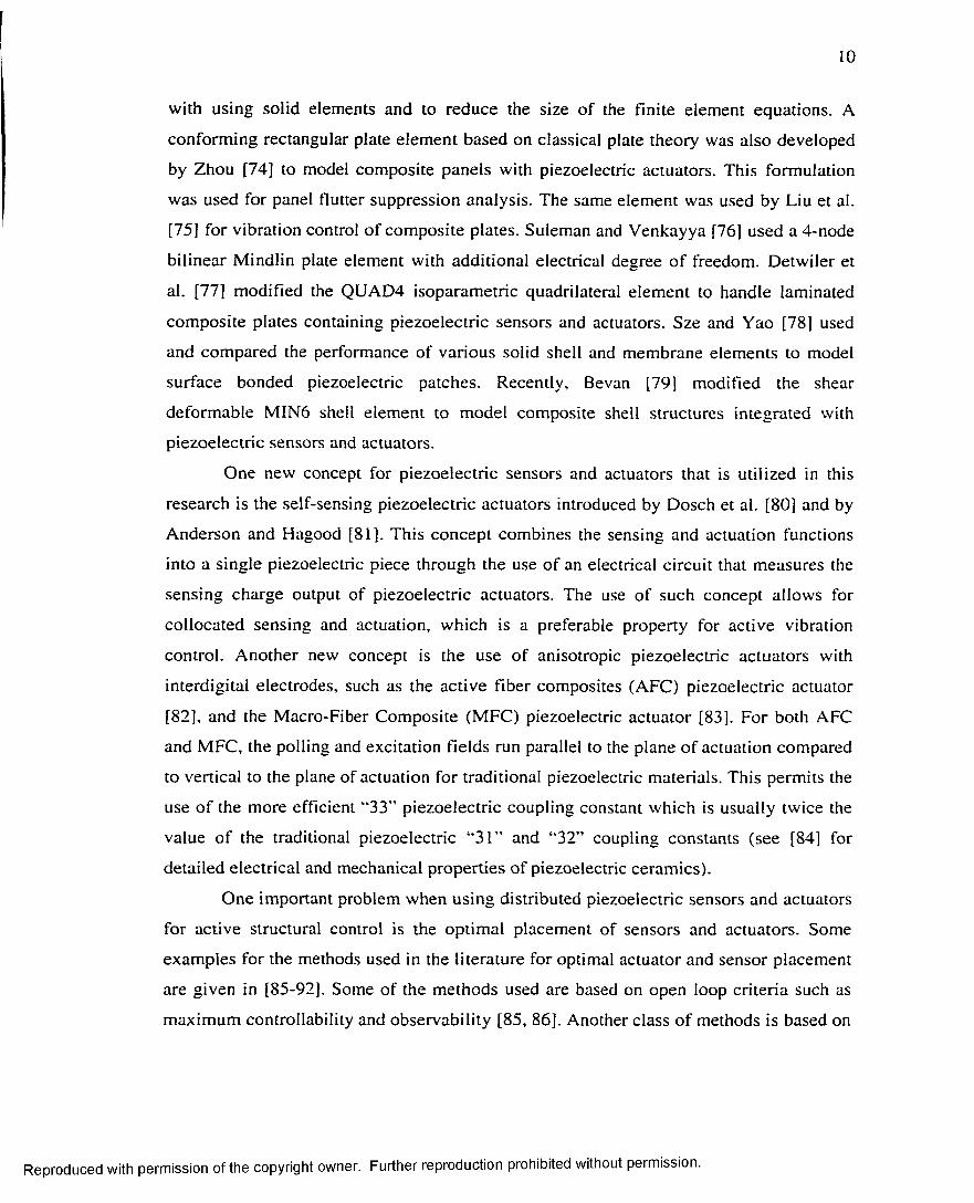
with using solid elements and to reduce the size of the finite element equations. A
conforming rectangular plate element based on classical plate theory was also developed
by Zhou [74] to model composite panels with piezoelectric actuators. This formulation
was used for panel flutter suppression analysis. The same element was used by Liu et al.
[75] for vibration control of composite plates. Suleman and Venkayya [76] used a 4-node
bilinear Mindlin plate element with additional electrical degree of freedom. Detwiler et
al. [77] modified the QUAD4 isoparametric quadrilateral element to handle laminated
composite plates containing piezoelectric sensors and actuators. Sze and Yao [78] used
and compared the performance of various solid shell and membrane elements to model
surface bonded piezoelectric patches. Recently, Bevan [79] modified the shear
deformable MIN6 shell element to model composite shell structures integrated with
piezoelectric sensors and actuators.
One new concept for piezoelectric sensors and actuators that is utilized in this
research is the self-sensing piezoelectric actuators introduced by Dosch et al. [80] and by
Anderson and Hagood [81]. This concept combines the sensing and actuation functions
into a single piezoelectric piece through the use o f an electrical circuit that measures the
sensing charge output of piezoelectric actuators. The use of such concept allows for
collocated sensing and actuation, which is a preferable property for active vibration
control. Another new concept is the use of anisotropic piezoelectric actuators with
interdigital electrodes, such as the active fiber composites (AFC) piezoelectric actuator
[82], and the Macro-Fiber Composite (MFC) piezoelectric actuator [83]. For both AFC
and MFC, the polling and excitation fields run parallel to the plane of actuation compared
to vertical to the plane of actuation for traditional piezoelectric materials. This permits the
use of the more efficient “33” piezoelectric coupling constant which is usually twice the
value of the traditional piezoelectric “31” and “32” coupling constants (see [84] for
detailed electrical and mechanical properties of piezoelectric ceramics).
One important problem when using distributed piezoelectric sensors and actuators
for active structural control is the optimal placement of sensors and actuators. Some
examples for the methods used in the literature for optimal actuator and sensor placement
are given in [85-92], Some of the methods used are based on open loop criteria such as
maximum controllability and observability [85, 86], Another class o f methods is based on
Reproduced with permission of the copyright owner. Further reproduction prohibited without permission.

II
minimization of a linear quadratic regulator (LQR) cost function using gradient
optimization methods [87-90]. A third class of methods is based on using more rigorous
optimization methods such as the genetic algorithm [91] and gradient based [92]
optimization techniques. More details for piezoelectric sensor and actuator placement for
the problem of panel flutter suppression will be discussed in the next subsection.
1.2.3 Panel Flutter Suppression Using Piezoelectric Materials
Many researchers have investigated the effectiveness of using piezoelectric
materials for passive or active control of flexible structures. However, only few studies
have been reported for linear and nonlinear supersonic panel flutter suppression using
piezoelectric materials. Scott and Weisshaar [93] were the first to study the suppression
of linear panel flutter using piezoelectric materials. The piezoelectric materials covered
the full surface of the panel and were used to generate bending moments to control panel
flutter. Four modes were retained using the Ritz method, and the panel was modeled as a
simply supported isotropic plate. Linear optimal control theory using full state feedback
LQR was employed in the simulation. Hajela and Glowasky [94] applied piezoelectric
elements in linear panel flutter suppression. Finite element models for panels with surface
bonded and embedded piezoelectric materials were generated to determine the response.
The actuation forces generated by the piezoelectric material were incorporated as static
prestress in the finite element models. Using a multi-criterion optimization scheme, the
optimal panel configuration with minimum weight and optimal sizing and layout of the
piezoelectric elements for maximum flutter dynamic pressure were determined. Using a
finite element approach, Suleman and Goncalves [95], and Suleman [96] recently
investigated a passive control methodology for linear panel flutter suppression. The
methodology induces tensile inplane loads from bonded or embedded piezoelectric
patches to increase panel critical dynamic pressure. They proposed the use of the physical
programming optimization method to determine optimal actuator configuration. Surace et
al. [97] used piezoelectric sensors and actuators to suppress linear supersonic panel flutter
using robust control techniques based on structured singular values for a simply
supported composite panel over a range of Mach numbers. The panel was modeled using
Galerkin’s method with classical plate theory and linear piston theory for aerodynamic
loading. Frampton et al. [98] employed a collocated direct rate feedback control scheme
Reproduced with permission of the copyright owner. Further reproduction prohibited without permission.

12
for the active control of linear panel flutter. The linearized potential flow aerodynamics
was used for the full transonic and supersonic Mach number range. They demonstrated
that a significant increase in the flutter boundary was achieved for a simply supported
square steel panel.
The first study of nonlinear panel flutter suppression using PZT piezoelectric
actuators was given by Abou-Amer [99]. He used piezoelectric layers to generate inplane
tension forces and consequently increase the panel flutter boundary. He showed that the
PZT material is more capable of preventing nonlinear panel flutter compared to using
active constrained layer damping. Lai et al. [100-102] studied the control of nonlinear
flutter of a simply supported isotropic plate using piezoelectric actuators. The Galerkin’s
method was adopted in obtaining the nonlinear modal equations. The optimal control
theory and numerical integration were used in the simulation. They concluded that the
bending moment induced by piezoelectric actuators is much more effective than inplane
forces for flutter suppression. Zhou et al. [103, 104] and [74] used the finite element
method to control isotropic and composite panels with surface bonded or embedded
piezoelectric patches. The finite element formulation considered coupling between
structural and electrical fields. An optimal full state feedback LQR controller was
developed based on the linearized modal equations. The norms of the feedback control
gain (NFCG) were used to provide the optimal shape and location of the piezoelectric
actuators. Numerical simulations showed that the critical flutter dynamic pressure is
increased about four times and two times for simply supported and clamped isotropic
panels, respectively. Dongi et al. [105] have presented a finite element method for
investigations on adaptive panels with self-sensing piezoelectric actuators. The
LUM/NTF algorithm was extended to include the linear and nonlinear active stiffness
matrices due to output feedback. A control approach based on output feedback for active
compensation o f aerodynamic stiffness (ACAS) terms is developed. They showed that
the ACAS control is able to increase the linear flutter boundary Mach number from =
3.22 to M e = 6.67 for a simply supported isotropic panel. Wind tunnel testing performed
by Ho et al. [106] has shown that panel limit-cycle motions observed in the wind tunnel
can be successfully reduced for composite panels with one-sided surface mounted
piezoelectric actuators and strain sensors using an iterative root locus based gain tuning
Reproduced with permission of the copyright owner. Further reproduction prohibited without permission.

13
algorithm. Their wind tunnel testing showed the leading edge piezoelectric actuator
patches to be more effective than the trailing edge patches in suppressing panel flutter.
Very recently, Kim and Moon [107] presented a comparison between active control and
passive damping using piezoelectric actuators for nonlinear panel flutter. The finite
element method was used to model the panel and LQR control method was used for
active control. The shape and location of the piezoelectric actuators was determined using
genetic algorithms.
With this exhaustive search for panel flutter suppression studies, two main
findings are determined. First, the effect of flow yaw angle has never been considered in
the literature for both linear and nonlinear panel flutter suppression, despite its great
effect on the panel flutter mode shape and, consequently, on the optimal location of
piezoelectric actuators and sensors. Second, most of the studies used LQR full state
feedback control assuming that all the states are available without any consideration for
the problem of state estimation for the nonlinear system dynamics or used non-optimal
output feedback based on iterative design methods.
1.3 Outline of the Study
This study presents multi-disciplinary research that includes nonlinear finite
element modeling of composite panels, aeroelasticity, modeling and optimal placement of
piezoelectric sensors and actuators, and control theory. It could be divided into two parts.
The first part covers finite element modeling and analysis for nonlinear flutter of
composite panels considering the effect of flow yaw angle and the effect o f additional
high acoustic pressure loading. The second part covers nonlinear flutter suppression for
composite panels under yawed supersonic flow using piezoelectric sensors and actuators
including optimal sensor and actuator placement and controller design.
The thesis is organized as follows. In Chapter 1, background material and
literature survey are given for the main topics of this research including nonlinear panel
flutter analysis, piezoelectric sensors and actuators, and panel flutter suppression
methodologies followed by an outline of the thesis contents. The derivation of finite
element coupled nonlinear equations of motion for composite panels with integrated
piezoelectric sensors and actuators under yawed supersonic aerodynamic flow and
acoustic loading is presented in Chapter 2 using the three-node triangular MIN3 plate
Reproduced with permission of the copyright owner. Further reproduction prohibited without permission.

14
element with improved transverse shear [48]. The MIN3 element is modified to handle
piezoelectric sensors and actuators by using an additional DOF for electrical potential per
each piezoelectric layer. In Chapter 3, modal transformation and reduction, and solution
procedure for nonlinear panel response are presented. The system governing equations
are transformed into the modal coordinates using the panel linear vibration modes to
obtain a set o f nonlinear dynamic modal equations of lesser order that can be easily used
to solve the problems of linear and nonlinear flutter boundaries and to analyze panel
response under combined acoustic and aerodynamic pressures. The reduced modal
equations o f motion are also used to design control laws and to simulate panel flutter
suppression. Solution procedures based on time domain numerical integration methods
and based on frequency domain methods for nonlinear panel flutter are also described in
this chapter. Validation o f the MIN3 finite element modal formulation and analysis
results are presented in Chapter 4. The MIN3 finite element modal formulation is
validated by comparison with other finite element and analytical solutions. Analysis
results for the effect of arbitrary flow yaw angle on nonlinear supersonic panel flutter for
isotropic and composite panels are presented using the frequency domain solution
method. In addition, the effect of combined supersonic aerodynamic and acoustic
pressure loading on the nonlinear dynamic response of isotropic and composite panels is
presented. Description of the different control methodologies used for nonlinear panel
flutter is presented in Chapter 5. Optimal control strategies [104] are the main focus for
the suppression of nonlinear panel flutter in this study. The linear quadratic Gaussian
(LQG) control, which combines both linear quadratic optimal feedback (LQR) and
Kalman filter state estimator, is considered as systematic linear dynamic compensator. In
addition, extended Kalman filter (EKF) for nonlinear systems [105-108] is also
considered and combined with optimal feedback to form a nonlinear dynamic output
compensator [109]. Finally, a more practical approach based on optimal output feedback
is used. Closed loop criteria based on the norm of feedback control gains (NFCG) for
actuators and on the norm of Kalman filter estimator gains (NKFEG) for sensors are
described to determine the optimal location of self-sensing piezoelectric actuators.
Simulation studies for the suppression of nonlinear panel flutter using piezoelectric
material under yawed supersonic flow are presented in Chapter 6 . Comparison of the
Reproduced with permission of the copyright owner. Further reproduction prohibited without permission.

15
different controllers considered is performed to determine the effect o f different control
strategies on the panel flutter suppression performance. In addition, results for nonlinear
panel flutter suppression under yawed supersonic for a specific range o f yaw angles,
including optimal actuator and sensor location, are presented for both isotropic and
composite panels. In Chapter 7, summary, conclusions, main contributions, and
recommendation for future work are given.
Reproduced with permission of the copyright owner. Further reproduction prohibited without permission.
16
Table 1.1 Panel Flutter Theories
Type Structure Theory Aerodynamic Theory Range of Mach No.
1 Linear Linear Piston V2 < Moo < 5
2 Linear Linearized Potential
Flow
1 < Moo < 5
3 Nonlinear Linear Piston y f l < Moo < 5
4 Nonlinear Linearized Potential
Flow
1 < Moo < 5
5 Nonlinear Nonlinear Piston Moo > 5
Table 1.2 Analogy between electrical and mechanical
variables for piezoelectric materials
Mechanical Electrical
Displacement u (vector) Electric Potential 0 (scalar)
Stress cr(2nd order tensor) Charge flux density (Electrical
Displacement) D (vector)
Strain f ( 2 nd order tensor) Electric field E (vector)
Reproduced with permission of the copyright owner. Further reproduction prohibited without permission.

Wni
ax/h
Flutter analysis Noise analysis
0.6
0.4
Dynanic Pressure, q
(4 , 1)
(0
mode (2,1)
mode (1,1)
Dynanic Pressure
Panel response Mode coalescence
A irflow
Flutter deflection mode shape for simply supported panel
i
0.5
0
0.5
1450 460 470 4 80 490 500
Tim e (msec)
Flutter limit-cycle oscillation
Figure 1.1 Explanation of nonlinear panel flutter phenomenon
Reproduced with permission of the copyright owner. Further reproduction prohibited without permission.

Polling direction
Applied or Sensed Electrical Field >
Surface electrodes
Figure 1.2 Schematic of traditional isotropic piezoelectric element
Reproduced with permission of the copyright owner. Further reproduction prohibited without permission.

19
CHAPTER II
FINITE ELEMENT FORMULATION
2.1 Introduction
The three-node triangular Mindlin (MIN3) plate element with improved
transverse shear, developed by Tessler and Hughes [52], is used in this study. This
element has Five degrees o f freedom per node and it uses a special interpolation scheme,
anisoparametric interpolation, to avoid the problem of shear locking commonly arising
when using the standard isoparametric interpolation approach. Additionally, an element-
appropriate shear correction factor is used to enhance element transverse shear energy.
Due to these improvements, the MIN3 element produces a well-conditioned element
stiffness matrix over the entire range o f thickness to length ratios. Based on extensive
numerical testing of the MIN3 element, Tessler and Hughes concluded that this element
is an excellent element for linear problems and is a very viable candidate for laminated
composites and nonlinear problems. Furthermore, Chen [53] demonstrated the efficiency
of this element for nonlinear problems by using it for the analysis of nonlinear panel
response under thermal and acoustic loading.
The MIN3 element is modified to handle piezoelectric sensors and actuators by
using an additional DOF for electrical potential per each piezoelectric layer. By doing
this, the modified MIN3 element becomes a fully coupled electrical-structure composite
plate element. The following are the main assumptions used in the formulation:
• Thin skin panels with embedded or bonded piezoelectric layers.
• Bending theory of Mindlin (first order shear deformation theory).
• Composite laminate theory.
• First order piston theory is used to model aerodynamic pressure for yawed
supersonic flow (1 .6 < Moo < 5).
• Large deflection effect is considered using nonlinear von-Karman strain
displacement relations.
• Linear constitutive relations for mechanical-electrical coupling are used
(linear piezoelectricity).
Reproduced with permission of the copyright owner. Further reproduction prohibited without permission.

2 0
In the following sections, the detailed derivation of the nonlinear dynamic equations of
motion for a laminated composite plate with embedded or bonded piezoelectric sensors
and actuators is given. The loads considered are aerodynamic pressure due to supersonic
yawed flow, random acoustic loading, and piezoelectric electrical loading (see Figure
2.1). This general system of coupled nonlinear equations will later be used to analyze
nonlinear panel flutter under yawed supersonic flow and nonlinear panel response under
combined aerodynamic and acoustic loading. In addition, these governing equations form
the basis for the design and simulation of control system design for nonlinear panel flutter
suppression.
Based on the Mindlin plate bending theory, the element displacement functions
are given by:
u x = u ( x , y , t ) + zip v (.v, y j )
u . = w ( x , y , t )
where u x, u y , u z are the displacement components at any point within the element; u, v, w
are the displacements o f the plate mid-plane; and y/x, i//y are the rotations of the mid-plane
normals due to bending only.
The electrical potential DOF is assumed constant for each piezoelectric layer; i.e.
w 0 is assumed constant over the element area.
2.2 Element Displacement Functions
u v = v(.v, y , / ) + z y / x (x, y , t ) ( 2 . 1)
w 0 (.v ,y , z , t ) = w tp ( z k , [ )
where Zk is the z coordinate o f the k lh piezoelectric layer.
Then the element degrees of freedom are defined as:
(2 .2 )
(2.3)
(2.4)
Reproduced with permission of the copyright owner. Further reproduction prohibited without permission.

2 1
where V is the electrical potential (voltage) for each piezoelectric layer and n p is the total
number o f piezoelectric layers per element (see Figure 2.2).
Displacement fields over the element are expressed in terms of element nodal
DOF and element interpolation functions as follows:
w(.v, y , 0 = 1H w J{wfc } + \_H w ¥ J{ p }
if/x ( x , y , t ) = [ / / « * - J M
iffy (x , y j ) = \ H m , ] f y / } (2 .5 )
u { x , y j ) = \ H u J {w „ ,}
v(.v, y , t ) = \_HV }
The element interpolation functions are expressed in terms of element area coordinates
(see Figure 2.3), and the element quadratic interpolation polynomials as given by
equation (2 .6 ).
f t f t j
f t l , m , m 2 Jl / v J = L « , , J = l i i * f t o o oj l/vJ=Ltf..J=L<> o o * f t f t j
Element area coordinates, 4i. are related to the element geometric coordinates using the
following transformation:
1 ~ l i i ' ’4 i.V • = x \ x 2 -r3 %2
. y . , y \ y 2 >’3.' ^ i i
1~ 2 A
x2>’3 - -v3-v2 .v2 - 3*3
rri1CO F
x 2 y i - ^ 1^3 V3 “ Vi x l ~ x 2 X
.^3 . .-vi -v2 ~ x 2 y \ -V1 _ .v2 x 2 ~ -VI . Vv. - J
(2.7)
where (x„y,) are the coordinates o f node /, and A is the triangular element area given by:
A = ^ ( x 2 —-vi )(y3 ~ >"i) — (-r3 ~ x 0 ( y i “ Vi)-
The element interpolation polynomials are defined as:
Reproduced with permission of the copyright owner. Further reproduction prohibited without permission.
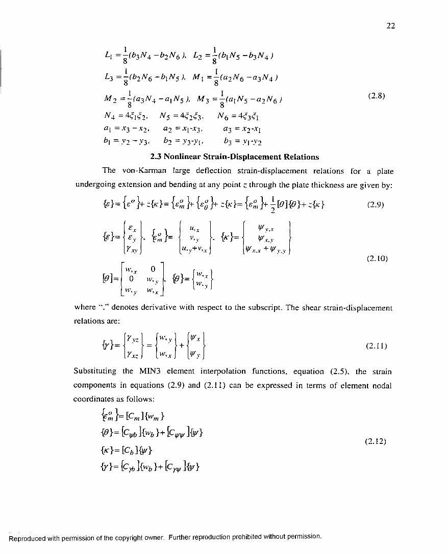
2 2
L x ~ — ( b 2 N 4 - b 2 N 6 ), L 2 = ~ ( b \ N 5 - b 2 N 4 )o o
L 2 = —( b 2 N 6 - b i N 5 ), M { = — ( a 2 N 6 - a 2 N 4 ) o o
M 2 = - ( a 2 N 4 - a { N $ ), M 3 = — ( a [ N 5 - a ^ i N f r ) 8 8
(2 .8 )
N 4 - 4 ^ \ q 2 < (V5 “ 4^2C3- ^ 6 = 4c3C[a { = x 2 - x 2 , a 2 = x x- x 3, = .v2 --V!
b \ = ,v2 ~ y 3 ’ b 2 = >*3-Vi, b 2 = >’i -V2
2.3 N onlinear S train-D isplacem ent Relations
The von-Karman large deflection strain-displacement relations for a plate
undergoing extension and bending at any point - through the plate thickness are given by:
{*}= {e" }+ ;{*}= y „ }+ { e " }+ ;{*}= { 4 }+ i [ e ] { S } + c M (2.9)
£ } = ■£ xe y - & , } =
u , xV.y ■. M = -
V y . x
V x . y
V X V u , Y+ v , x V x . x + V y . y
[«] =W , x 00 vv, v
IV, v VV’, r
(2 . 10)
vv,,VV.,
where denotes derivative with respect to the subscript. The shear strain-displacement
relations are:
y yz w , v V x- = ■
- M >
Yxz v v \ r V vI '
( 2 . 11)
Substituting the MIN3 element interpolation functions, equation (2.5), the strain
components in equations (2.9) and (2.11) can be expressed in terms of element nodal
coordinates as follows:
& ^Pif/b ]{lvfc \p y / y / ]{(^}
M = [ Q J M
{ / } - \C y b ]{wfc }+ \ C y V ]{^}
(2 . 12)
Reproduced with permission of the copyright owner. Further reproduction prohibited without permission.

where the strain interpolation matrices are given by equations (2.13) through (2.16).
[C, „ ]= L H V ± y
.L^vJvv+L^./ J’V(2.13)
(2.14)
(2.16)
(2.15)
Expressions for these strain interpolation matrices as functions o f element geometry and
area coordinates are given in Appendix A.
Based on the analogy given in chapter 1 between electrical and mechanical
quantities for piezoelectric materials, the electrical field-potential relations are analogous
to mechanical strain-displacement relations. Assuming that the electrical degrees of
freedom are constant over each piezoelectric layer in the element, the electrical field is
related to the electrical DOF by:
Both traditional isotropic piezoelectric materials and anisotropic piezoelectric actuators,
such as active fiber composite (AFC) [82] and macro-fiber composite (MFC) [83], are
covered by the presented formulation. For isotropic piezoelectric materials, the
polarization direction is the ‘"3” direction; consequently, {E,} is the electrical field in the
3 direction and /i( is the thickness of the piezoelectric layer. For anisotropic piezoelectric
2.4 Electrical Field-Potential Relations
(2.17)
Reproduced with permission of the copyright owner. Further reproduction prohibited without permission.
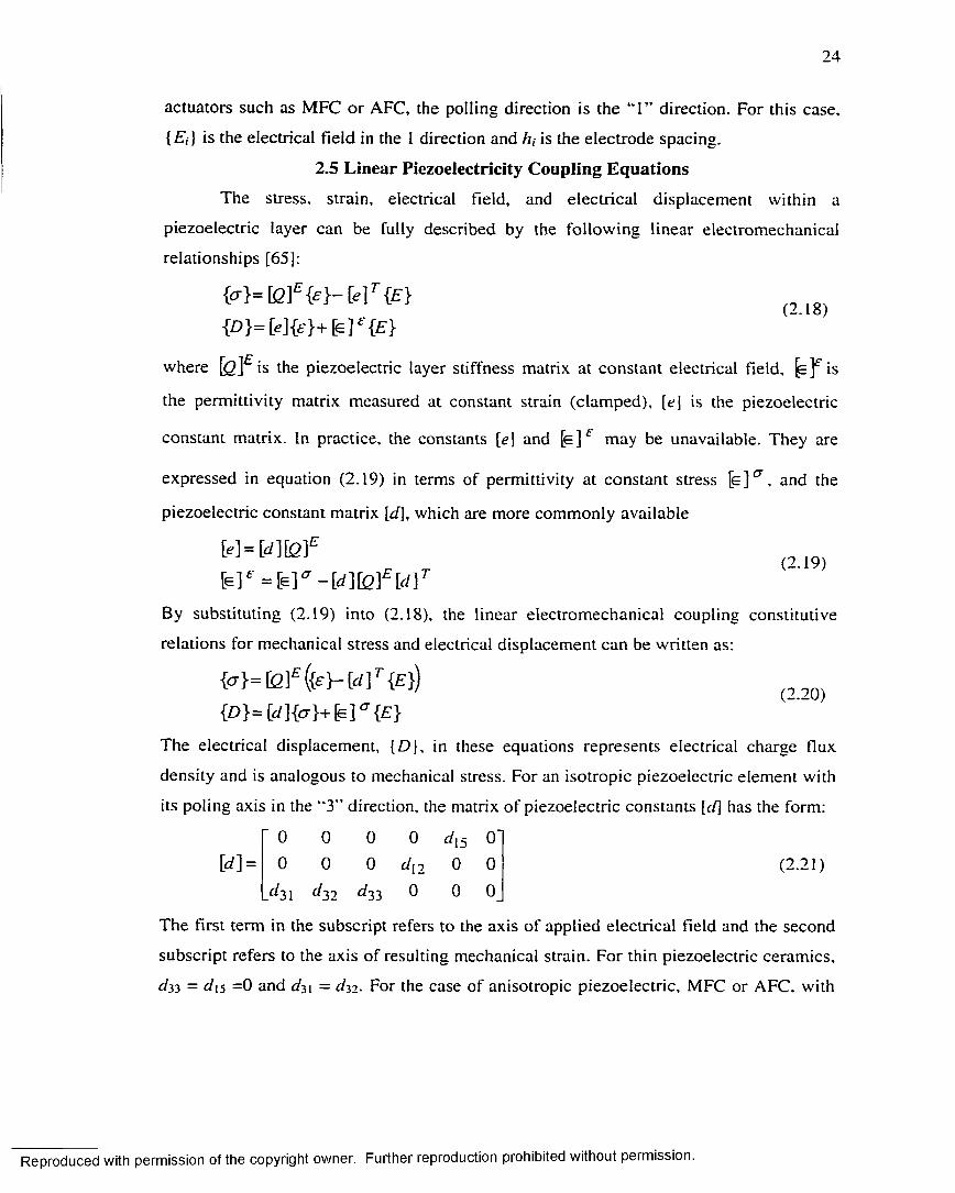
24
actuators such as MFC or AFC, the polling direction is the “ 1” direction. For this case,
{£,} is the electrical field in the 1 direction and h i is the electrode spacing.
2.5 Linear Piezoelectricity Coupling Equations
The stress, strain, electrical field, and electrical displacement within a
piezoelectric layer can be fully described by the following linear electromechanical
relationships [65]:
(, Ig){£>}=[e]£r}+[e]f {£}
where \q Y " is the piezoelectric layer stiffness matrix at constant electrical field, is
the permittivity matrix measured at constant strain (clamped), [e] is the piezoelectric
constant matrix. In practice, the constants [e] and [ e ] f may be unavailable. They are
expressed in equation (2.19) in terms of permittivity at constant stress [e]*7 , and the
piezoelectric constant matrix [ d \ , which are more commonly available
[ e ] = [ d ] \ Q ) E(2.19)
[e ] f = [ G ] a - [ d ] [ Q ] E [ d ] T
By substituting (2.19) into (2.18), the linear electromechanical coupling constitutive
relations for mechanical stress and electrical displacement can be written as:
M = [ f i ] £ ( fr H r f]r {E}) (, 90){ D } = fc /]M + fe ]CT{£}
The electrical displacement, {D}, in these equations represents electrical charge flux
density and is analogous to mechanical stress. For an isotropic piezoelectric element with
its poling axis in the “3” direction, the matrix of piezoelectric constants [r/] has the form:
' 0 0 0 0 d \ 5 00 0 0 d \ 2 0 0
.^31 ^32 d 33 0 0 0
The first term in the subscript refers to the axis of applied electrical field and the second
subscript refers to the axis of resulting mechanical strain. For thin piezoelectric ceramics,
< 33 = d is =0 and d j i = <32. For the case of anisotropic piezoelectric, MFC or AFC, with
Reproduced with permission of the copyright owner. Further reproduction prohibited without permission.

25
the poling axis in the “ 1” direction, the constants d - u and d 32 are replaced by d \ \ and d \ 2
which are determined experimentally [83].
2.6 Constitutive Equations
Lamina stress-strain relations are derived based on the Mindlin plate theory and
on the linear electromechanical piezoelectric coupling equations. It is assumed that all
laminas are perfectly bonded with zero glue thickness. For a laminated fiber reinforced
composite panel with embedded or bonded piezoelectric layers, the kth layer stress-strain
relationships in the material principal axes (1,2,3) are given by:
(2 .22 )0-1 Qw 012 0 n
/’ £\ d i\
\O’ 2 • = 012 0T> 0 * e2 ' - E a t - d i2 •
r12. k 0 o' 066. k y 12 0
The klh layer could be either structure lamina (£,* = = 0) or piezoelectric layer. The
transverse shear stress-strain relations are also given by:
^ 23! _r13 J*
<244 0 . 0 055
V23
k(2.23)
For regular isotropic piezoelectric layers i = 3, corresponding to applied or sensed
electrical field in the “3” directions while for MFC or AFC piezoelectric actuators / = 1,
corresponding to applied or sensed electrical field in the *T” direction.
In laminate reference axes (x, y, z), the constitutive equations are:
(2.24)' O n 012 016
/d x
\
• = 012 022 026 £ y ~ E ' k ’ d y •
k 016 026 066 k Y x \ d xy k >
| r .v: 044 045' K \l r -vc.K = 045 055. t 1
(2.25)
(2.26)
In matrix compact format these equations can be written as:
{<7}t = E l ({<?}-£,*{<*},)
where, \ Q ] and \ Q S ] are the lamina transformed reduced stiffness matrices for plane
stress and transverse shear respectively, and { d } is the transformed piezoelectric
Reproduced with permission of the copyright owner. Further reproduction prohibited without permission.

26
constants vector. Details of the derivation of transformed stiffness and piezoelectric
constants using laminated composite theory are given in Appendix B.
In addition to mechanical stress, the electrical displacement o f piezoelectric
layers, given in equation (2 .20), can be written as:
D« = ¥ 1 ( t?} - E i t ¥ \ E ik (2.27)
Thus, equations (2.26) and (2.27) represent the constitutive relations for a general
composite lamina or a piezoelectric layer.
2.7 Laminate Resultant Forces and Moments
In a general composite laminate, stress is different from one layer to another. The
resultant stresses for the laminate, or forces and moments per unit length, are obtained by
integrating stress over the laminate thickness, h, as:
h! 2({w }{M })= J{cr}t ( I , : ) *
- h i 2hi 2
{*}= J H d z
(2.28)
- h t 2
Using the lamina constitutive relations, the force and moment resultants are written as:
"A B ~ £ ° N 0
B D . K A V (2.29)
where the laminate extension, extension-bending, bending, and shear stiffness matrices,
[A], [£], [ D ] , [A5], are defined as:
/i/2
(M,[fl].[0]) = J leU ,:,:2}/;—h i 2
h / 2 _[ A J = \ \ Q s \ d z
- h / 2
and the piezoelectric resultant force and moment are:
h / 2 _
( K ) . W } ) = \ \ Q \ { d } k E l t ( l , z ) d z- h / 2
(2.30)
(2.31)
Reproduced with permission of the copyright owner. Further reproduction prohibited without permission.

27
These force and moment resultants can be expressed in terms of element nodal DOF
using equation (2 . 12) for { ? } and { k }, and equation (2 .17) for E ik as follows:
{W}= [A][C„, ]{«-„ }+2- M[0]( [c*, ] k }+ [c„ ]fcr})+ [B}[Cb }
{M}= [J][C.]{,, }+Y&ttajflc*, I k }+ [c„ ]M)+[o][c,, }{«}= [ a , j[c ]k }+ [4S ][cw ]K
(2.32)
and the resultant piezoelectric force and moment as:
K F - k -i [bJ K IV }= ~ \-P m ]
where the piezoelectric matrices [TV] and [ P m ] are defined as:
KJ=[lcl{rf},A, - IQ\{d\hk ... \5 lp{d}„ph,v ]
= ... E l - K K w - ; * ) 2 (2.34)
[i2 \ i p I — )” J
2.8 Aerodynamic Pressure Loading
Assuming an airflow that is parallel to the panel surface, the aerodynamic
pressure loading is expressed using the first-order piston theory. This theory relates the
aerodynamic pressure and panel transverse deflection as follows:
(2.33)}= 1 feJW }
A P a = -2 qa
J3' . M i - 2 1 A
vv, r c o s a + w , .. s in a -i ---------------w .rM i - l V „
(2.35)
where q a = p a V z /2 is the dynamic pressure, p a is the air density, V „ is the airflow
velocity, vv is the panel transverse displacement, is the Mach number, a is the flow
yaw angle, and /? = y j M i - 1 . Using non-dimensional parameters, equation (2.35) can
be written as:
A — [vv, v cos a + w, v sin a ] + — l~ w, tA P a = “
where
f r> - _ „ r » \(2.36)
a 3 o a 4 j
Reproduced with permission of the copyright owner. Further reproduction prohibited without permission.

28
, _ 2 q a a Z _ p a V x { M l - 2 )Rr\ ’ 3 a ~P D 110 p h ( D 0 ( j
(2.37)
are the non-dimensional dynamic pressure, non-dimensional aerodynamic damping,
aerodynamic damping coefficient, and panel reference frequency, respectively. Duo is the
first entry of the laminate bending stiffness matrix [D] determined with all fibers of the
composite layers are in the x-direction as a reference, p , a , and h are the panel density,
length and thickness, respectively.
Equation (2.36) shows that the aerodynamic loading on the panel is function of
both local panel slopes in the .v and y directions and of the panel vibration velocity;
therefore panel flutter is a self-excited vibration. Using the MIN3 element interpolation
functions, the aerodynamic pressure can be expressed in terms of element nodal DOF as
follows:
2.9.1 Generalized Hamilton’s Principle
Element matrices and nonlinear coupled electrical and structural equations of
motion for a composite laminated plate element with piezoelectric layers are derived
using the generalized Hamilton’s principle. In addition to aerodynamic loading, a random
surface pressure is also considered to allow the study of panel response under combined
aerodynamic and acoustic loading. The generalized Hamilton’s principle is:
where T is the kinetic energy, U is the strain energy, W eiec is the electrical energy, and
W e.xt is the work done by externally applied forces and electrical voltage. These energy
terms are defined by the following volume integrals:
(2.38)
( L t f » J K } + ! « » • * > } )2.9 Element Equations of Motion and Matrices
(2.39)
(2.40)Vol “
Reproduced with permission of the copyright owner. Further reproduction prohibited without permission.

29
^ = J \ { e } T (2.41)Vol ~
K l « = / (2.42)Vol
The work done by external forces and voltage is given by the surface integrals:
W e x t = J iw7 iFs } I S - J (2.43)5, S2
where {Fs} represents the surface loading on the element due to aerodynamic pressure
and acoustic pressure, 5/ is the area of the surface loading. V is the applied voltage, p iS is
the surface charge density of the piezoelectric layer, and S 2 is the area of piezoelectric
layer. All variations at times // and t 2 must vanish in the Hamilton’s principle, and thus it
can be written as:
V° l (2.44)+ { S e Y {£> } ]r/V + J {<5W}r { F s y i s - J S V p c s d S = 0
Si s 2
The element matrices are determined by evaluating equation (2.44) term by term to arrive
at the element nonlinear dynamic equations of motion.
2.9.2 Element Stiffness and Electromechanical Coupling Matrices
Element stiffness matrices including piezoelectric electromechanical coupling
terms are derived using the variation of strain energy and electrical energy terms.
S t r a i n E n e r g y :
Using the definition of stress force and moment resultant, the strain energy variation term
can be written as:
S U = 7 {^1+ { S f c f { M }+ a s {S y f (2.45)
where a s is the MIN3 element shear correction factor, which is defined as function of the
ratio of the diagonal shear and bending stiffness coefficients associated with the
rotational degrees of freedom:
Reproduced with permission of the copyright owner. Further reproduction prohibited without permission.

The exact definition of element shear and bending stiffness matrices will be given later.
More details about the selection of the shear correction factor are given in [52].
Substituting for strain and stress resultants in terms of element interpolation matrices and
element nodal DOF into equation (2.45), the strain energy variation can be expressed as:
*/ = J {({&■„, }r [c,„ f + {&■„ }r [cVi, r rnT + {Svf [c„ F l e f )
[A][c,„ ]{»•„, } + - [A ][s ] [c f* ] K }
+ {[A][0][cw ]fr}+[S][C (, ]{(ir}+ [/>* ][«„ I K }]
(2.46)
+
^[B][<9][C^ ]{¥ }+ [D][Cb ]{¥ }+ [PM ] [B0 ]{w0 }
as ({ v’6 }T \Cyb Y + {V}r \cw F )(U, ] [Cyt ]{wb }+ U , ] [Cw ]{¥ }) }dA
(2.47)
(2.48)
Electrical Energy:
By substituting equation (2.27) for electrical displacement, the variation of electrical
energy can be written as:
r i i /2 t ~ \ "■ 5 W W = J £ t t )</: (2.49)
A L-/j / 2
Using the definition of piezoelectric matrices [/V] and [Pa/], the electrical energy
variation becomes:
S W elei. = J { 5 E ( }r ( [ P , v f f M + K I K { £ / } ) < « ( 2 .5 0 )
where the new piezoelectric matrix [P<,] is defined as:
Reproduced with permission of the copyright owner. Further reproduction prohibited without permission.

31
0 e ?^ Itfip
0
- U V „ P \ Q l p V htn p
(2.51)
Using the strain-displacement relations, the electrical energy variation can be expressed
in terms of nodal DOF as follows:
= j l s T K F [Jvf [cm]{wm}+-[e][cvb]{w6}A 1 ^
+ ^ [e ] [c „ » ,]M )+ [P M f [ Q , ] M + M K } l d A
(2.52)
J J
The linear and nonlinear element stiffness and electromechanical coupling matrices can
be found now from the variation of both strain and electrical energies by writing the sum
of S U and S W eiec in matrix form as follows:
S w b T '0 0 08 y / 0 [ * v }\pni
S w ni*
0 [ k \n i tp [ k ] m
S w 0K
0 \.k]<pip \-k \0m
0 [ ^ ' i h ip [ ^ 1 h m [ * l k
[ ^ 1 \ipb [*iV [^•1 \tpm U'lV[^■11 mlp 0 0
}<pb [ ^ • i h ip 0 0
o n [ k s ]b V 0 0 "
[k] <P0+ a . [ ^ • s 1 ipb [ k s 1 \p 0 0
+[k] m 0
j0 0 0 0
[ k ] 0 _ 0 0 0 0
" [* . v 0 h \-k\N 0 hip 0 o '
+ \.k\tf(t) \yjb r * i w V 0 0+
0 0 0 00 0 0 0
(^•1 Nm h h \p 0 o ' \ - k \N b h tp 0 o '
t^-' l Nm Jipb h 0 0+ tpb \-k\N iA ip 0 0
0 0 0 0 0 0 0 00 0 0 0 0 0 0 0 _
+
~ i k 2 \b \.k2 h ip 0 0 " >w b
[ k 2 ]ipb [ k 2 \v 0 0 ¥
0 0 0 0 w m0 0 0 0
/w<p
= S U + d W elec (2.53)
where the element sub-matrices in equation (2.53) are defined by the following equations.
Reproduced with permission of the copyright owner. Further reproduction prohibited without permission.

32
L i n e a r s t i f f n e s s s u b - m a t r i c e s :
[ k ] w = \ [ C b ]T [ D ] [ C b ] d A (2.54)<4
= \ [ C b ]T [ B ] [ C m ) d A = [ k \ Tm ¥ (2.55).4
[*]„, = j [ C m f [ A ] [ C m ]clA (2.56)A
P i e z o e l e c t r i c c o u p l i n g s u b - m a t r i c e s
[ k \ „ I0 = \ [ C m \ T [ P N \ [ B 0 ] d A = [ k ] l n (2.57)A
[* W = l [ C b ]T [ P M ] [ B 0 ] d A = [ k \ l ¥ (2.58)A
P i e z o e l e c t r i c c a p a c i t a n c e s u b - m a t r i x
{ k \ o = \ [ B 0 \ T [ P 0 \ d A (2.59)A
S h e a r s t i f f n e s s s u b - m a t r i c e s
[ k s ]b = $ [ C } b ]T [ A s }[C. r b ] d A (2.60)A
\ .k s \b i/ / = \ [ C y b i r \ .As \ [ C y ¥ ] d A = \ k s (2.61)A
[ k s V = J [ C w ]r [As. ][Cm lcM (2.62)A
F i r s t - o r d e r n o n l i n e a r s t i f f l e s s m a t r i x
The following nonlinear element sub-matrices are first order functions of the element
transverse displacement through [ 6 \
1[ k x \ b v = ~ \ i C v b ]T { 6 } T [ B ] [ C b ] d A = [ k x ] T¥b (2.63)“ A
I k i h , , , = ^ \ [ C ¥ b ]T [ d } T { A ] [ C m ] d A = [ k l ]Tmh (2.64)
A
1
A
[*ilr = ^ f i C b ] T [ B ] [ e ] [ C W9, \ d A + J [ C ^ ] r [0]r [fi][C6kM (2.65)“ A A
[*1 W = ]^A = [* ,]«* (2 .66)A
Reproduced with permission of the copyright owner. Further reproduction prohibited without permission.

33
F i r s t - o r d e r p i e z o e l e c t r i c c o u p l i n g m a t r i c e s
The following nonlinear element sub-matrices are first order functions of the element
transverse displacement through geometric matrix [ 6 \
[ * i W = ^ J [ c V J r [ 0 ] 7> / v ] [ S 0 ] < M = [ * , & ( 2 - 6 7 )
[ t i U = { p N \ { B 0 \ d A =[A,1 r<P¥ (2 .68)
The following nonlinear element sub-matrices are first order functions of the element
electrical displacement through piezoelectric resultant force {Af<j}.
= - \ \ [ C v h]T [N0 }[Cv/b)dA
C T T[ * l i V 0 — — T j [ A 0 \[CVV \clA —~ A
t W V = - ^ \ { C v v \T [ N0 ][C¥ ¥ ]dA
( 2 . 6 9 )
( 2 . 7 0 )
( 2 . 7 1 )
where the force resultant matrix [A is found from the force resultant vector (Ar) as
follows:
N xN v , M = ( 2 . 7 2 )
First-order nonlinear stiffness m atrix due to { N , „ }
The following sub-matrices are first-order nonlinear functions of plate membrane
displacement {vv„,} through the membrane resultant force {A/„, }=[/!]{
1 * 1 Atm = ^ l i C ¥ b \ T i N m \[C„f b \dA ( 2 . 7 3 )
\btff — 7 f lCi /rbl [A * ] [C W \dA — [ A r i^ ~
l A / „ , 1 1 \dA
( 2 . 7 4 )
( 2 . 7 5 )
F i r s t - o r d e r n o n l i n e a r s t i f f n e s s m a t r i x d u e t o { N b }
The following sub-matrices are first-order nonlinear functions of plate rotational
displacement { \ p \ through the membrane resultant force {A/b }=[#]{ k ]
Reproduced with permission of the copyright owner. Further reproduction prohibited without permission.

34
l*i,v* h = ^ - J i c vb lT I N b ] [C vb \dA~ A
1*1 Nb h<y = \T [ N b \ [ C VV I dA = \ ^ b“ A
I k \Nb V = | j t C W ? l N b II'C W 1 ^
(2.76)
(2.77)
(2.78)
S e c o n c l - o r d e r n o n l i n e a r s t i f f n e s s m a t r i x
The following nonlinear element sub-matrices are second-order functions of the element
transverse displacement through geometric matrix [ 6 \
1*2 U = - \ [ C ¥ b ]r [ 0 \ T [ A \ [ e \ [ C y b \dA
1*2 W via = [ k 2 \ lb~ A
1*2 V = \T \ e \ T [ A w e w C y y VIA
(2.79)
(2.80)
(2.81)
2.9.3 Element Mass Matrices
Element mass matrices are determined using the variation of kinetic energy term
in the generalized Hamilton’s principle. Using MIN3 element interpolation function, the
kinetic energy variation can be written as
s r = { p h { { S » - m }r ( { H „ }LH „ J { .v „ , } + { H v } |W „ })A
+ k&vb f iH w }+ W f {h wy/ })( LH w ]{Swb }+ L" w y ^ } % iAEquation (2.82) can be written in matrix form as:
(2.82)
S T =
SwbT
M b I ' » V 0 O'S i y I I™]#, [ m ] v 0 0 V
S wm 9 0 0 [ '” 1 m 0 w ,n5 w 0 0 0 0 0 <v0
(2.83)
where the element mass sub-matrices are defined as:
[ m ] b = J l w „ . /a
I '« W = j l " W J
(2.84)
(2.85)a
Reproduced with permission of the copyright owner. Further reproduction prohibited without permission.
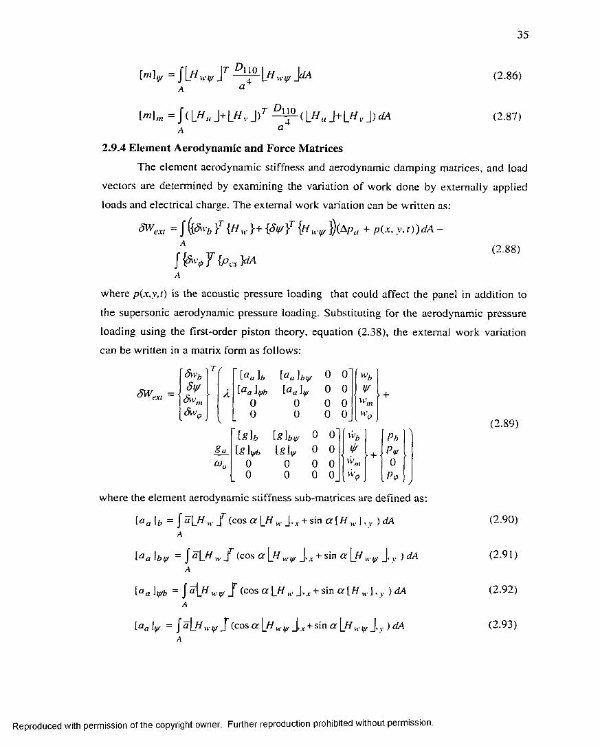
35
Imiy = JL«,v.„J7' ^ !j 2-L« ,,« ,> >
D,
(2.86)a
(2.87)[m ]„ , = J ( L ff„ J + I H „ J ) r - U 5 . ( LH u ] + l H , ] ) d A
<4 “
2.9.4 Element Aerodynamic and Force Matrices
The element aerodynamic stiffness and aerodynamic damping matrices, and load
vectors are determined by examining the variation of work done by externally applied
loads and electrical charge. The external work variation can be written as:
SW ext = J ({^ V'Z> } T i H u-}+ {H wifr })(AP</ + P U , y , t ) ) d A -
(2 .88 )J Y { P c s )d A
where p ( x , y , t ) is the acoustic pressure loading that could affect the panel in addition to
the supersonic aerodynamic pressure loading. Substituting for the aerodynamic pressure
loading using the first-order piston theory, equation (2.38), the external work variation
can be written in a matrix form as follows:
s w ^ = \
Swb t f
8y/ XSwm
\-a a 0 0 * w b
[c*a lysb \.a a ^l// 0 0 V
0 0 0 0 w m0 0 0 0 WP
Sa_CD,,
[j> \bt/f 0 o' w b Pb\
[.? 1 if/b [S 1 y/ 0 0 V • -1- - Plf/►
0 0 0 0 00 0 0 0 _ LP 0 /
(2.89)
where the element aerodynamic stiffness sub-matrices are defined as:
\ b = { a \ J f w J (cos a \ _H w J, v + sin a [ H w ], v ) d A A
\.a a 1b !]/ ~ \ c i [ H lt, (COS DC \_H _), x ^ in CX [_ // wiff _|» v )
A
[« a \ y b = J a\_H wl// J (cos a \_H w J ,x + sin a [ H w J , v ) dAA
[ a a V = J H W v J (cos a \_H w w J,x + sin a | H u. v J, v, ) clA
(2.90)
(2.91)
(2.92)
(2.93)
Reproduced with permission of the copyright owner. Further reproduction prohibited without permission.

36
The element aerodynamic damping matrices are the same as element bending mass
matrices given by equation (2.84) through (2.86)
[ § ~ \ . m \ b ' \ -S \b i f / \ .§ \ y / = (2.94)
Finally, the element load vectors due to acoustic random pressure and applied electrical
charge are defined as:
\ P b }= J [ Hj p ( x , \ \ t ) d AA
(2.95)
\ p v } = \ [H p ( x * y , t ) d AA
(2.96)
W }= “ J K j }dA (2.97)A
For the case of panel flutter analysis and suppression, the acoustic pressure. p ( x , v , t ), will
be set to zero. However, some of the analysis cases given in Chapter 4 will consider the
combined effect of acoustic loading and supersonic aerodynamic pressure.
2.9.5 Element Equations of Motion
Using the element stiffness, mass, aerodynamic matrices and load vectors, the
fully coupled nonlinear electromechanical equations of motion for a composite laminate
with piezoelectric layers subject to supersonic aerodynamic and acoustic loading using
the MIN3 element can be written as:
’ ["*k [ m ] h v 0 0" ii'b ~ [ g \ b [«? \btf/ 0 0‘[ m \ v 0 0 ¥ ■ + — ti> \if/b 0 0 ¥
0 0 0 V o 0 0 0 0 vvm0 0 0 0 0 0 0 0 w 0
(1-®a ^blf/ 0 o ' ' 0 0 0 0 1
A \-a a ]tf/b 0
t aci 0
0
0
0
0+
0
0^l//0 +
V0 0 0 0 0 [ k ] 0 _
~ [ k s ]b \b y / 0 o ' 0 \bi f / [*•'1 h r n t ^ ' l I b 0
cc j }y/b [^•5 0 0 [ * I [ * i V t ^ - l ]y/ni [ ^•1 \y /0
0 0 0 0 [*1 h n b [ ^ 1 \m ij/ 0 0
0 0 0 0 _ [ ^ 1 \<pb [ 1 \0 \jf 0 0
Reproduced with permission of the copyright owner. Further reproduction prohibited without permission.

37
N 0 f^"IN<p ^bif/ 0 o ' 0 0 '
\.^ \N 0 ^ ip b 0 0+ 0 0
0 0 0 0 0 0 0 00 0 0 0 0 0 0 0
[ 'lA! b h t 'lA'b h i / / 0 o ' [ •2 [^2 W 0 0 w b P b[ k \ N b \ y b [ k [ Nb V 0 0 + [^2 ]y/f> [*2V 0 0 ¥ __ Ptft
0 0 0 0 0 0 0 0 w m 00 0 0 0 0 0 0 0 / P q
One important thing to note for this equation is that, all element matrices are symmetric
except the aerodynamic stiffness matrices, which are skew symmetric. For abbreviation
from now on, the element bending DOF {vry,} and { y / \ are combined together in a single
vector. Thus, the 4 matrices with subscripts b , b y / , y /b , and y/a re all combined in a single
matrix denoted with the subscript b .
2.10 System Equations of Motion
The system equation of motion for the complete plate can be found by following
the standard finite element assembly, and using the specified structural and electrical
boundary conditions. The electrical DOF also follows the traditional finite element
assembly procedure where the electrical boundary condition stipulates equal potential
across element boundaries for each continuous piezoelectric patch. Using the new
notation for bending DOF:
f o } = 2 b } (2.99)all elenints *■ '
where the summation sign represents the finite element assembly procedure. Combining
the shear and linear bending stiffness matrices in a single stiffness matrix [AH, then the
system equations of motion for a composite panel embedded with piezoelectric layers and
subject to supersonic aerodynamic pressure and acoustic pressure can be written as:
\ M b 0 0" g ~Ga 0 o ' W b '0 M m 0 ■ W m 0 0 0 W m - +0 0 0
%u 0 0 0 0 %
/ "A* 0 o'~ Kb ^bni
1 1£ < 0 o '
A 0 0 0 + Knib Km K/)10 + 0 0 0V
0 0 0 1 * % K<pm 0 0 0
Reproduced with permission of the copyright owner. Further reproduction prohibited without permission.

38
K \ b + K \ Nm + K 1NbK lK \
mbpb
K l b m00
ATIbp00
K 2 0 0 0 0 0 0 0 0
w b Pb- = ■ 0
Pp(2 . 100)
where [A/], [ G aJ, [ A a ], and [AT] are the system mass, aerodynamic damping, aerodynamic
stiffness and linear stiffness matrices, respectively; [ATI] and [ K 2 ] are the first-order and
second-order nonlinear stiffness matrices, which are linear and quadratic functions of the
unknown displacements { W b } and { W , „ } respectively; and [ K 1 n 0] is the piezoelectric first
order stiffness matrix which depends linearly on the electrical DOF { W 0 }. In the absence
of acoustic pressure loading, { P b } = 0, equation (2.100) reduces to the problem of
nonlinear panel flutter under yawed supersonic flow. However, by setting A and g a to
zero, equation (2 . 100) describes nonlinear random response of composite panels
subjected to high acoustic excitations. The formulation is kept in a general form with
both effects to allow the study of nonlinear panel response under combined acoustic and
aerodynamic loading. However, {P/,} will be dropped when nonlinear panel flutter
analysis and control are considered.
2.11 Piezoelectric Actuator and Sensor Equations
The system equation (2.100) represents a system of coupled electrical-structural
nonlinear equations. Collecting the structure degrees of freedom {W b ) and {W m ] in one
vector denoted as {Wj, equation (2 . 100) can then be simplified as follows:
( 2 . 101)
M 00 0
K 2 0
fA
'A O'+ ~ K W
r
+V 0 0 _%V i
Av0 ) | / 0 J
Any piezoelectric layer in the composite laminate could be used as a sensor, actuator, or a
self-sensing actuator. First, the case of a plate equipped with piezoelectric sensors and
actuators is examined, then the case of self-sensing piezoelectric actuators.
2.11.1 Piezoelectric Material as Actuators and Sensors
For this case it is assumed that each piezoelectric patch is either used as a sensor
or as actuator. The electrical DOF are partitioned into sensor DOF and actuator DOF, or a
sensor voltage vector and an actuator voltage vector as follows:
Reproduced with permission of the copyright owner. Further reproduction prohibited without permission.
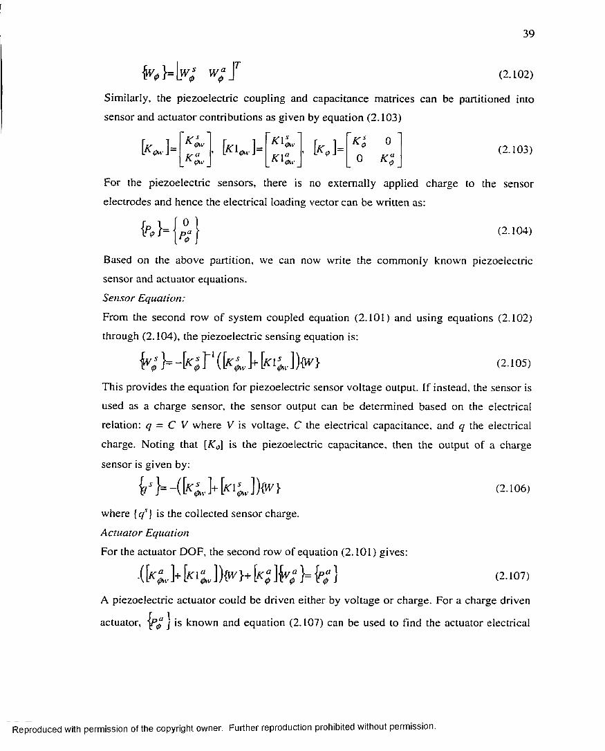
39
(2. 102)
Similarly, the piezoelectric coupling and capacitance matrices can be partitioned into
sensor and actuator contributions as given by equation (2.103)
0
K(2.103)
For the piezoelectric sensors, there is no externally applied charge to the sensor
electrodes and hence the electrical loading vector can be written as:
r o(2.104)
Based on the above partition, we can now write the commonly known piezoelectric
sensor and actuator equations.
S e n s o r E q u a t i o n :
From the second row of system coupled equation (2.101) and using equations (2.102)
through (2.104), the piezoelectric sensing equation is:
K 1 }= - f a F ' ( J+ 1 * 1 ] ){l4,> < 2 i 0 5 )
This provides the equation for piezoelectric sensor voltage output. If instead, the sensor is
used as a charge sensor, the sensor output can be determined based on the electrical
relation: q - C V where V is voltage, C the electrical capacitance, and q the electrical
charge. Noting that [K\>] is the piezoelectric capacitance, then the output of a charge
sensor is given by:
{ l ‘ }= - f e . 1+ f c l j J V } (2 - >06)
where { q * } is the collected sensor charge.
A c t u a t o r E q u a t i o n
For the actuator DOF, the second row of equation (2.101) gives:
•([* > ,]+ [k ; }= £ > /] (2.107)
A piezoelectric actuator could be driven either by voltage or charge. For a charge driven
actuator, ] is known and equation (2.107) can be used to find the actuator electrical
Reproduced with permission of the copyright owner. Further reproduction prohibited without permission.

40
DOF { w ° ] as a function of the structural DOF {W } and the known applied charge as
follows:
K ° 1= f a J"1 { f a } - ( f a , ]+ f a * . ] M (2- io s )The actuator electrical DOF is then substituted in the first row of equation (2.101) to
obtain the actuator equation for a charge driven actuator. However, in the usual actuator
application, a driving voltage is used instead of a charge. In this case, the actuator
voltage ] is known and the charge drawn onto the piezoelectric electrodes in response
to this voltage is not o f interest. Therefore, equation (2.107) is ignored. For the voltage
driven piezoelectric actuator, the actuator equation can be written as follows:
—-^-[M }+ -^ -[G ]^V J+ (A [A ]+ [^ ll.]+[^'l]+[AT2 ] ){W }= { P } + { P a c l }(2.109)c o - u 0
where {Facr} represents the piezoelectric force due to the voltage at both sensor and
actuator and is given by:
{P a c , > = - ( f a . * ] + f a t * ] ) f a M f a * ] + f a t * ] ) K “ J < 2 -1 10 >
Since the actuation voltage is much bigger than the sensor voltage, the sensor term in
equation (2 . 110) is neglected and the actuator equation for a voltage driven actuator is
finally given as:
- y [ M ] }+ [ G ] }+ ( A [ A ] + [ K w ]+ [ K 1]+M o 01 o (2 .111)
l K 2 ] ) { 1 V } = { P } - ( f a * ] + f a i t * ] ) f a }
2.11.2 Piezoelectric Material as Self-Sensing Actuators
For these devices, each layer of piezoelectric material is used as sensor and
actuator simultaneously. Therefore, there is no need to partition {W 0 ] for this case.
Equation (2.101) can be then written as two separate equations to represent actuation and
sensing as follows:
—V [ M ] } + [ G ] f y } + ( A [ A ] + [ K w ]+ [ATI]co ~ M a (2 . 112)
+ [JC2 ] ) { W }= {/>}- ( fa „ * ]+ f a l ] ) f a ]
Reproduced with permission of the copyright owner. Further reproduction prohibited without permission.

41
(2.113)
The key to self-sensing piezoelectric actuators is measuring the electrical charge drawn to
the electrodes, ( P 0} . This electrical charge can then be combined with the piezoelectric
capacitance and applied electrical voltage, the term [ K P] { W 0 ) in equation (2.113), to get a
signal proportional to the structure DOF. Analog circuits such as the ones given in [80]
and [81] can be used to implement the right hand side of equation (2.113). In practice, the
compensation for the piezoelectric capacitance is not perfect and could affect the sensor
performance. In this study, the difference between the piezoelectric capacitance and the
electric circuit compensation will be neglected, i.e., perfect implementation of the right
hand side of equation (2.113) is assumed. Therefore, the sensor output charge for self
sensing piezoelectric actuators is given by:
Thus, equations (2.112) and (2.114) are the actuator and sensor equations, respectively,
for self-sensing piezoelectric actuators.
(2.114)
Reproduced with permission of the copyright owner. Further reproduction prohibited without permission.

42
Acoustic pressure
Yawedsupersonicflow Bonded or embedded
Piezoelectric layers
Composite laminate
Figure 2 .1 Composite panel under yawed supersonic flow and acoustic pressure loading
Reproduced with permission of the copyright owner. Further reproduction prohibited without permission.

43
Zn-t-1
ZlZ2
{W*} = {VU..., Vk Vnp}
i
/ "
i1
\\jr
np
vk
x-►
V,
Piezoelectric layers
Figure 2.2 Composite laminate composed of n layers with n p piezoelectric layers
Reproduced with permission of the copyright owner. Further reproduction prohibited without permission.

44
(x2, y2)
(x l , y l ) { i» ^2,^3} = {Ai, A2, A3}/A A = ZAj
Figure 2.3 MIN3 element geometry and area coordinates
Reproduced with permission of the copyright owner. Further reproduction prohibited without permission.

45
CHAPTER III
MODAL REDUCTION AND SOLUTION PROCEDURE
3.1 Introduction
The nonlinear dynamic equations derived in the pervious chapter represent the
equation of motion in the structural node DOF. These equations could be used to solve
nonlinear panel response for flutter and combined aerodynamic and acoustic loading.
However, it is not efficient to do so due to the large number of structure node DOF and
due to the nonlinear stiffness matrices, which have to be updated. Additionally, a reduced
order system that only retains the important modes of the system should be used for
control system design.
In this chapter, the system governing equations are transformed into the modal
coordinates using the panel linear vibration modes to obtain a set of nonlinear dynamic
modal equations o f lesser number. The reduced modal equations can be easily used to
solve the problems of linear and nonlinear flutter boundaries and to analyze panel
response under combined acoustic and aerodynamic pressures. Linear and nonlinear
panel flutter problems can be solved using either time domain methods such as numerical
integration, or frequency domain methods (eigenvalue problem solution). However, the
problem o f nonlinear panel response under combined aerodynamic and acoustic loading
must be solved using time domain methods. The reduced modal equations o f motion will
also be used to design control laws and to simulate panel flutter suppression. The
following are the main assumptions used in the modal reduction and solution procedure:
• General composite laminate, symmetric or unsymmetric.
• Inplane inertia is neglected. This is justified as the frequencies of inplane
vibration modes are much higher frequency than the out of plane bending modes.
• Self-sensing piezoelectric actuators are assumed. Therefore, equations (2.112) and
(2.114) represent the coupled actuation and sensing equations, respectively.
• The piezoelectric actuators bonded to the surface or embedded within the
laminate produce only bending moment and not inplane force. In other words, the
piezoelectric resultant force, is zero. This is achieved by having a pair of
Reproduced with permission of the copyright owner. Further reproduction prohibited without permission.
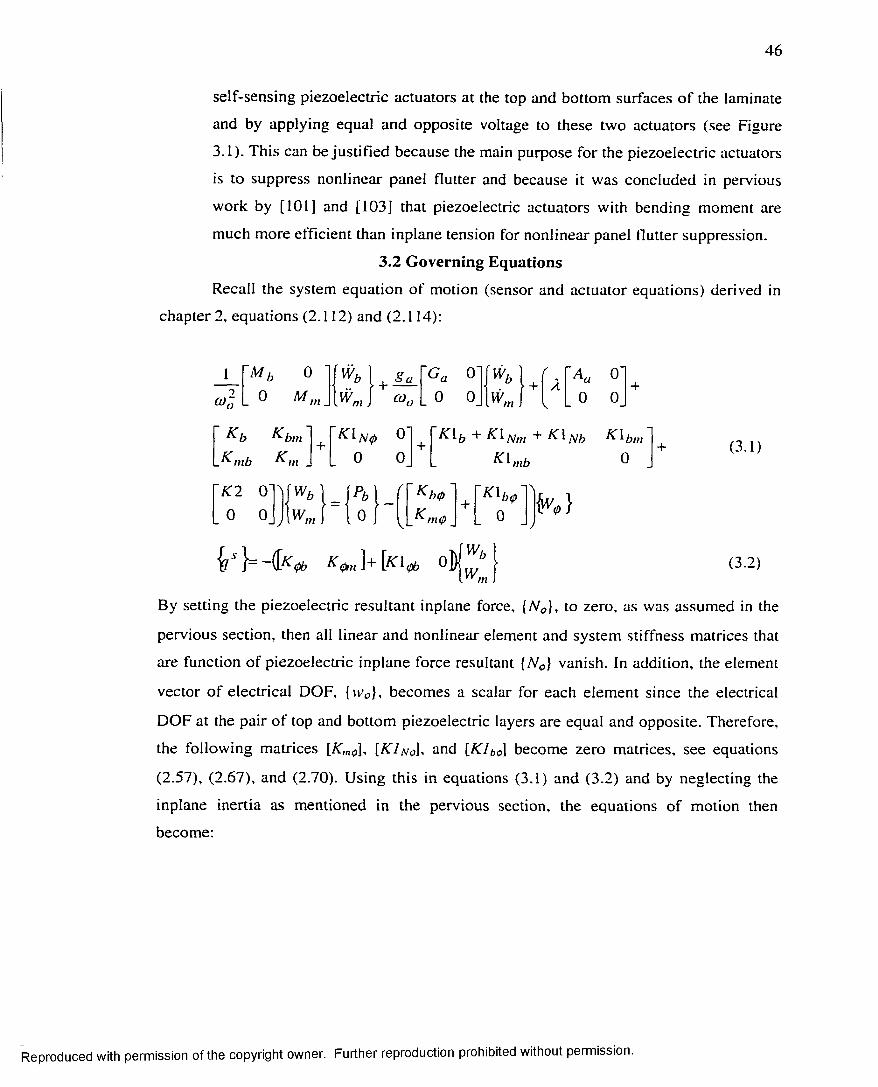
46
self-sensing piezoelectric actuators at the top and bottom surfaces of the laminate
and by applying equal and opposite voltage to these two actuators (see Figure
3.1). This can be justified because the main purpose for the piezoelectric actuators
is to suppress nonlinear panel flutter and because it was concluded in pervious
work by [101] and [103] that piezoelectric actuators with bending moment are
much more efficient than inplane tension for nonlinear panel flutter suppression.
3.2 G overning Equations
Recall the system equation of motion (sensor and actuator equations) derived in
chapter 2, equations (2.112) and (2.114):
M b0
0
' K b
K m b
K 2 0 0 0
K bm+
K m J
>1- ) 1 w (I vy m J
W h
W ,+
mS a CO,
~Ga O' { * b \ 1+(/I o'
_ 0 0 K , J 0 0_K l N <p o
o
P b
o+
K \ b + K i Nm + K \ Nb
K 1 mb
+
+ (3.1)
f K b0+
1
5 C-
____
_J \
V 1 > I
0 JK )
'Wu
\ W ,(3.2)
m
By setting the piezoelectric resultant inplane force, {yV<j}, to zero, as was assumed in the
pervious section, then all linear and nonlinear element and system stiffness matrices that
are function of piezoelectric inplane force resultant [A^] vanish. In addition, the element
vector o f electrical DOF, {vv'0}, becomes a scalar for each element since the electrical
DOF at the pair o f top and bottom piezoelectric layers are equal and opposite. Therefore,
the following matrices [ATra()], [ K 1 n 0 \ , and [K l b0] become zero matrices, see equations
(2.57), (2.67), and (2.70). Using this in equations (3.1) and (3.2) and by neglecting the
inplane inertia as mentioned in the pervious section, the equations of motion then
become:
Reproduced with permission of the copyright owner. Further reproduction prohibited without permission.

47
~ M b O ' \+8“ ~Ga o 'R L(
A X ,O '
+~ K b K bm
_ 0 0 _ R, °>o 0 0 R, [ \ 0 0 . K nib K m .
A c t u a t o r E q u a t i o n :
11
U o
' K \ b + K \ N m + K \ N b
mb
S e n s o r E q u a t i o n :
+
~ K 2 O' j+
J . 0 0 /' W hw,m
' R. o f
K b 00 K ) <3-3>
W = - k * o fo l ^ lW',„f
(3.4)
It is worth mentioning that the pure transverse displacement sensor signal in equation
(3.4) is obtained by summing the charge outputs from the pair of top and bottom
piezoelectric layers (see Figure 3.1). Equation (3.3) can be partitioned to two separate
equations for bending and inplane DOF. The inplane DOF, {W,„}, can be expressed in
terms of the bending DOF, { W h \ . as:
{ W ,„ }= I" ' ([£„,(, ! + ( « ,„ ; , I) { W b } (3.5)
and the system equations in terms of the bending displacement { W i,} as:
- L . [ M b ] ^ b Y — [ G a 1R H ([*J + [ K n l 1) i w b }= { P b R ] R }(3.6)CO~ W o
where the linear and nonlinear stiffness matrices are given by:
[ K l 1 = ( i [ A a ] + [ K b \ ~ [ K b m \ { K m ]- { [ K m b ]) (3.7)
(3.8)[Kfl /L 1 - - [ K b m 1 I K^mb 1 + ) +
+ [ K 2 \ - [ K i b m \ [ K m ] - l ( [ K m b \ + [ K l m b \)
The system equation of motion in structural DOF, equation (3.6), has two major
drawbacks. First, the element nonlinear stiffness matrices have to be evaluated and the
system nonlinear stiffness [ K ^ l \ is assembled and updated at each iteration or numerical
integration step. Second, the number of structure node DOF {W b) is usually very large
which is not suitable for control laws design and computationally costly for both
frequency domain and time domain solution methods. To overcome these drawbacks, the
system equations are reduced using modal transformation and modal reduction based on
the values of modal participation. This results in a system of coupled nonlinear modal
Reproduced with permission of the copyright owner. Further reproduction prohibited without permission.

48
equations with much lesser number of DOF that could be used for control design,
numerical integration, and frequency domain solution.
3.3 Modal Transformation and Reduction
Assuming that the panel deflection can be expressed as a linear combination of
some known function as
K } = i > r (D{0r }=[<!>]{<7} (3.9)r= I
where the number o f retained linear modes n is much smaller than the number of
structure node DOF in bending, {W b ) . The normal mode {$-}, which is normalized with
the maximum component to unity, and the linear natural frequency cor are obtained from
the linear vibration of the system.
c o r 2 [ M b ][<pr ) = [ K b ]{<t>r } (3.10)
Since the nonlinear matrices [ K l mb\, [K l bm], [ K l Nb], and [ K 2 ] are all function of the
unknown bending DOF { W b } , they can be expressed as the sum of products of modal
coordinates and nonlinear modal stiffness matrices as
( [ K l „ l b l [ K \ b m \ [A Tl^]) = ^ q r i K \ m b ]( r \ [ K l b fJ r>, [ K l tWb1 r>)
(3’l l )
r = I j = 1
where the super-indices of those nonlinear modal stiffness matrices denote that they are
assembled from the corresponding element nonlinear stiffness matrices. Those element
nonlinear stiffness matrices are evaluated with the corresponding element components
[ w b } {r ) obtained from the known system linear mode {<j)r }- Therefore, those nonlinear
modal stiffness matrices are constant matrices. This is a great advantage, as these
matrices do not need to be evaluated at the element level and assembled at each iteration
or time integration step.
The first-order nonlinear stiffness matrix [A7m„] is a linear function o f the inplane
displacement { W „ ,} . From equation (3.5), {W m ) consists o f two terms as:
Reproduced with permission of the copyright owner. Further reproduction prohibited without permission.

49
Y q r [ K \ m b ] ^ U ] { « } l r = l J (3.12)
n n n
= ' S Cli'{0r}m ~ ^ ^ c l r c l s (0r.v I w r= i r= l 5=1
where the two inplane modes corresponding to the r-th bending mode {<pr } are defined as:
Thus, the nonlinear stiffness matrix [ K I Nm\ can be expressed as the sum of two nonlinear
modal stiffness matrices as:
[* l/v » .]= -2 > < -[K l/v » ,f r) (3.14)r = 1 r = l , v = l
The nonlinear modal stiffness matrices [ K l Nm](r) and [K 2 Nm ](rs> are assembled from the
corresponding element nonlinear stiffness matrices. Those element nonlinear stiffness
matrices are evaluated with the corresponding element components obtained from
the known inplane modes {#-},„ and {0„}m, respectively. Thus, the nonlinear modal
stiffness matrices are constant matrices. Using equations (3.11) and (3.14), the system
equation, (3.6), is transformed to the following reduced nonlinear system in the modal
coordinates
- V [ M b ^ | c ]{<)}+ 2 { r <or [/ ]& }+C0o CO- (3.15)
( Ik l 1+ K ] + [ x m ] ) { q } = & h [ ic b ( , ] { j y „ }
And the sensing equation in the modal coordinates is:
{7 5 } = - [ ^ f e } (3.16)
As for the electrical DOF, there is no need to do reduction since the number of electrical
DOF, { W 0 ) , is usually small.
The modal matrices are given by:
® v 7 j , [ C ] , [ ^ ] ) = [ 0 f ( [ M 6 ],[C ],[ /i:L ])[cI)l (3.17)
and the quadratic and cubic terms in modal coordinates are:
Reproduced with permission of the copyright owner. Further reproduction prohibited without permission.

50
K ]= [<*>f £ qr ][Arm r 1 [/nm61‘1+mb r> -[KiNm t ‘r =1 (3.18)
+[K1 Nb 1rl - [K\bm f r) [K m r 11 [Kmb ])[4>]
n n[k w ] = t-f f s s ‘u M " ' r ' -
r= l„ l (3.19)
[Kif,„,]<r» [*:mr ,[ i„,1>]<),)[0]and the modal load vector and piezoelectric control force are:
\ F b }= W {P h } (3.20)
[ ^ ] = t < i - r k j = [ ^ r (3.2i)
The nonlinear first order modal matrix [AT(/] usually represents a softening effect while the
second order nonlinear matrix [ K qq] represents a hard spring or stiffening effect. For the
special case of symmetric panels, [ K q \ is zero (due to [B ] = 0) and the modal equations of
motion reduces to a multi DOF coupled Duffing system. Structural damping modal
matrix, [ c ] = 2 £ r a ) r ( M r / c o ^ ) [ l ] , has been added to the system modal equation (3.15)
where £ r, Q)r, and M r are the modal damping, frequency, and mass, respectively, and [/] is
the identity matrix. The modal damping ratio can be determined based on testing or on
performance of similar structures.
The advantages of the modal equations of motion given by equation (3.15) are: (i)
there is no need to assemble and update the nonlinear stiffness matrices at each iteration
since all the nonlinear modal matrices are constant, and (ii) the number of modal
equations is much smaller than the structure equations. This approach has been
successfully used for nonlinear panel flutter of composite panels at elevated temperature
by Zhou et al. [104]. This approach has also been demonstrated for nonlinear panel flutter
of composite panels under yawed supersonic flow by Abdel-Motagaly et al. [51] and for
nonlinear response of composite panels under combined acoustic and aerodynamic
loading by Abdel-Motagaly et al. [64],
The determination of the number of modes required for a specific problem is not a
trivial task and requires some special attention to make sure the important modes are
Reproduced with permission of the copyright owner. Further reproduction prohibited without permission.

51
retained. The few influential modes to be kept can be determined by the modal
participation value, which is defined as:
For the problem o f nonlinear panel flutter, the number o f modes used can be determined
based on accurate and converged magnitude and frequency of limit-cycle oscillation
(LCO). By doing this, it is guaranteed to get accurate flutter mode shape, which is crucial
for panel flutter suppression problem. For the problem of acoustic loading in the form of
uniform random pressure input, the lowest few symmetric modes are usually used. In
summary, modal reduction is problem dependent and should be performed based on a
systematic modal convergence and participation procedure.
3.4.1 Time Domain Method
Nonlinear panel response could be simply solved by using numerical integration
of the modal dynamic equations of motion. For the case of combined loading, the random
surface pressure is generated and the panel response is determined at each time step. For
the case of nonlinear panel flutter, numerical integration is carried out using any arbitrary
initial conditions at a given value of nondimensional dynamic pressure, A . After some
time, the solution converges to a limit cycle and the limit cycle oscillation (LCO)
amplitude and frequency can then be determined at the given A . This approach is accurate
and general as it could easily handle both structural and aerodynamic damping. However,
the frequency domain solution introduced in the next subsection is more effective
computationally for the case of nonlinear panel flutter when the interest is only to
determine the panel LCO response and the flutter mode shape. For control design and
simulation, numerical integration must be used.
3.4.2 Frequency Domain Method
3.4.2.1 Critical Flutter Boundary
Linear panel flutter equations of motion can be determined by neglecting the
nonlinear stiffness matrices, and by setting the piezoelectric actuation and random surface
pressure to zero in equation (3.15).
P a r t i c i p a t i o n o f t h e r - t h m o d e = \ q r \ / Ski (3.22)
3.4 Solution Procedure
Reproduced with permission of the copyright owner. Further reproduction prohibited without permission.

52
[ M b M + ^ [C ]{?}+ 2C r O r [/]{?}+ W L ]fe}= {0}CO
(3.23)
This equation represents a dynamic eigenvalue problem and a solution for the unknown
modal coordinates {q ) can be assumed in the form of:
where [ q , , ] is the eigenvector and Q = 0 + i c o is the panel motion parameter (J.3 is
damping rate and co is frequency). Flutter will occur if the panel motion becomes
unstable, i.e., when the damping rate becomes positive. Using the fact that [G] = [M h \ and
neglecting the structural damping, the linear panel flutter eigenvalue problem can be
written as follows:
where the eigenvalue, Kj, is defined in terms of aerodynamic damping and reference
frequency as:
As the nondimensional dynamic pressure, A , increases, the panel symmetric stiffness
matrix will be perturbed by the skew symmetric aerodynamic matrix (see equation (3.7)
for the definition of [Aj.]). This will result in one eigenvalues K) to increase and another
eigenvalue K j to decrease until they coalesce. If A is increased further, the two
eigenvalues become complex conjugate:
For the case of zero aerodynamic damping, g a = 0, the damping rate is zero at the
coalescence of the two eigenvalues and hence this defines the flutter critical boundary,
A cr , (i.e. at Ki - 0). In the presence of aerodynamic damping, the damping rate will vanish
after the coalescence. Substituting (3.26) into (3.27) and using the definition of Q, it is
found that 0 = 0 when Ki/ K r = g a . The value of A cr in the presence of aerodynamic
damping is thus slightly higher than that with no aerodynamic damping. Based on linear
theory, the panel motion will grow exponentially beyond A cr_ In reality, this is not the
case due to inplane stretching forces. Thus, the nonlinear matrices must be considered to
(3.24)
(3.25)
X/.2 — Kr + I K i (3-27)
Reproduced with permission of the copyright owner. Further reproduction prohibited without permission.

53
determine the panel limit-cycle oscillation (LCO) response beyond the critical flutter
boundary.
3A.2.2 Nonlinear Flutter Limit-Cycle Oscillation
The reduced nonlinear modal equations for the nonlinear eigenvalue problem of
panel flutter could be solved using the linearized updated mode with nonlinear time
function (LUM/NTF) approximate method introduced and applied by Gray [11] for
nonlinear hypersonic panel flutter and by Xue [39] for nonlinear supersonic panel flutter.
The LUM/NTF method is an iterative method. It was originally applied in the structure
node DOF and thus requires evaluation and assembly of element matrices at each
iteration. An efficient solution procedure, presented here for the first time, is to apply the
LUM/NTF method to the reduced modal equations. The presented solution procedure is
efficient and has a great advantage in computation time and thus could be used for the
study of nonlinear LCO amplitude and for flutter mode shape determination of composite
panels.
The LUM/NTF solution procedure is based on using harmonic response
assumption and on linearization of nonlinear time functions. Since the intent is to
determine LCO amplitude and frequency, the solution of the modal DOF is assumed in a
harmonic form similar to equation (3.25):
{<y}= { q 0 = { q 0 } ( c o s c u t + i s i n c o t ) (3.28)
Using equation (3.15), the nonlinear panel flutter eigenvalue problem can be written as
follows:
( - K j [ M b ]+ \ K L ]+ [ K q ]+ [if w ] ){ ,„ = {0} (3.29)
For a stable limit cycle, the modal solution in equation (3.28) can be written by setting /?
to zero and by choosing either cos(tu t ) or sin(ry t ) for the harmonic solution. Using this
modal solution, equation (3.29) becomes:
(- K j [m b ]cos cut + cos cut + \ fC q ]cos 2 cut + [K q q ]C°S3 O x ) { Q o }= {0} (3.30)
Using linear approximation for the nonlinear time functions (cos2cut and cos3tuf), the
linearized eigenvalue problem for LCO of nonlinear panel flutter can be written as:
Reproduced with permission of the copyright owner. Further reproduction prohibited without permission.
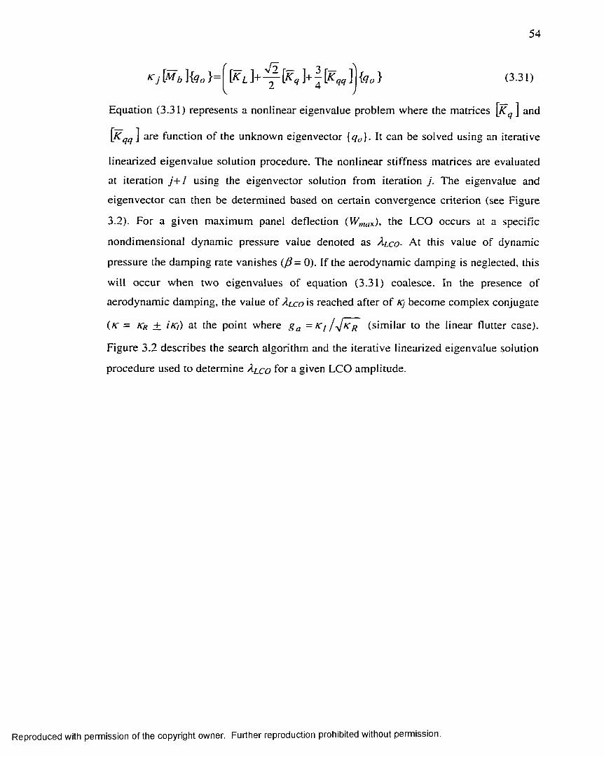
54
2 4v y
Equation (3.31) represents a nonlinear eigenvalue problem where the matrices \ K q ] and
[ K q q ] are function of the unknown eigenvector { q 0 }- It can be solved using an iterative
linearized eigenvalue solution procedure. The nonlinear stiffness matrices are evaluated
at iteration j + I using the eigenvector solution from iteration j . The eigenvalue and
eigenvector can then be determined based on certain convergence criterion (see Figure
3.2). For a given maximum panel deflection ( W m a x ) , the LCO occurs at a specific
nondimensional dynamic pressure value denoted as A l c o - At this value of dynamic
pressure the damping rate vanishes (/? = 0). If the aerodynamic damping is neglected, this
will occur when two eigenvalues of equation (3.31) coalesce. In the presence of
aerodynamic damping, the value of A l c o is reached after of Kj become complex conjugate
( k = K r ± iK i ) at the point where g a = * 7 1 4 K R (s im ile to the linear flutter case).
Figure 3.2 describes the search algorithm and the iterative linearized eigenvalue solution
procedure used to determine A ^ c o for a given LCO amplitude.
Reproduced with permission of the copyright owner. Further reproduction prohibited without permission.

Sensor chargesoutput, q
Self-sensing piezoelectric actuators
W62= - W4>1
Figure 3.1 Configuration of self-sensing piezoelectric actuators for bending
moment actuation and transverse displacement sensing
Reproduced with permission of the copyright owner. Further reproduction prohibited without permission.

56
S t e p I : For a Given LCO amplitude W m a x , Assume {q a}
S t e p 2 : Assume a value for X
S t e p 3 : Solve the linearized eigen equation for the j-th iteration:
K j \ M b ] (< ? o } j = ( [ ^ z . ] + [ ^ N L } y
[K N L . ] = ^ - [ K q f e o } j _ ! ) ] + ^ \K qq } j - [ ) ]
where { q 0 }j is the updated modal solution
S t e p 4 : Get { W h \ from { q „ } } using { W b ] = [ 0 ] ( q „ a n d Find ( W ntax) j
then adjust { q „ ) j to result in the required W max using:
r -i r i ( ^ m a x ) g iv e nh o i i - h o i j - M — T—
v r max / j
S t e p 5 : Test for convergence of {r/„}, if not go to step 3
S t e p 6 : Check for coalescence of the eigenvalues:
- if not, A = A + A A then go to step 2
- if yes A l c o = A then exit
Figure 3.2 Iterative solution procedure for nonlinear panel flutter limit-cycle response
Reproduced with permission of the copyright owner. Further reproduction prohibited without permission.

57
CHAPTER IV
FINITE ELEMENT ANALYSIS RESULTS
4.1 Introduction
Validation of the MIN3 finite element modal formulation and analysis results are
presented in this chapter. The MIN3 finite element modal formulation is validated by
comparison with other Finite element and analytical solutions. The validation tests
performed include: linear free vibration, piezoelectric static actuation, linear and
nonlinear panel flutter, time and frequency domain solutions, and nonlinear panel
response under random acoustic pressure loading.
Using the verified MIN3 Modal formulation, analysis results for the effect of
arbitrary flow yaw angle on nonlinear supersonic panel flutter for isotropic and composite
panels are presented using the frequency domain solution method. The effect of
combined supersonic aerodynamic and acoustic pressure loading on the nonlinear
dynamic response of isotropic and composite panels is also considered.
Results are presented for isotropic material (Aluminum) and for graphite/epoxy
Fiber reinforced composite with different laminate stacking sequence. The properties of
the different materials used in this chapter are given in Table 4.1. As for the panel
geometry, the MIN3 triangular element is used to model square, rectangular, and
triangular panels using different mesh sizes. Figure 4.1 shows a typical MIN3 finite
element mesh used to model both rectangular and triangular panels.
4.2 Finite Element Validation
4.2.1 Natural Frequencies
The First validation test is comparing the First few natural frequencies versus
analytical values for a simply supported square isotropic panel performed to verify the
linear stiffness and mass matrices. The panel dimensions are 12x12x0.05 in.,
corresponding to panel length, a , panel width, b , and panel thickness, h , respectively. The
analytical natural frequencies (rad/s) are determined using the classical plate theory
solution and are given by:
Reproduced with permission of the copyright owner. Further reproduction prohibited without permission.

where D = -— . Table 4.2 show the first six natural frequencies calculated using12(1- 1/ - )
equation (4.1) and a 12x12 MIN3 Finite element mesh (total of 288 elements). It can be
seen that the difference between the MIN3 solution and analytical solution is less than
0.5%.
4.2.2 Piezoelectric Static Actuation
The piezoelectric finite element formulation is validated using the cantilevered
bimorph beam shown in Figure 4.2 (symmetric half o f the beam). The bimorph beam
consists of two identical PVDF piezoelectric layers with polling axis in the 3 direction
but with opposite polarities. Hence, this beam will bend when electrical field is applied in
the vertical direction. The mechanical and electrical constants for PVDF are given in
Table 4.1. A unit electrical voltage is applied across the thickness and the beam lateral
deflection at different points is determined. The results obtained using a 5x2 MIN3
elements mesh are compared against the analytical solution of [69], the solid finite
element of [78], and the QUAD4 finite element of [77]. Table 4.3 shows that the
deflections obtained using the MIN3 element formulation are in good agreement with
other analytical and finite element solutions.
4.2.3 Linear and Nonlinear Flutter
The MIN3 modal finite element solution using the lowest 25 modes and a 12x12
mesh is used to compare the critical nondimensional dynamic pressure, A cr, values versus
the CQ conforming quadrilateral element solution [46] and analytical solutions [15] for
simply supported isotropic rectangular panels with different aspect ratios and at different
flow yaw angles. All solutions assume zero aerodynamic damping and A c r is
nondimensional with respect to the panel length, a . Table 4.4 shows that, the solution of
the MIN3 modal formulation is in very good agreement with the CQ element and with
the analytical solution for different aspect ratios and different flow angles with maximum
difference of less than 2%.
Reproduced with permission of the copyright owner. Further reproduction prohibited without permission.

59
The limit-cycie oscillations (LCO) response for a simply supported (with
immovable inplane edges) square (12x12x0.05 in.) isotropic panel with zero yaw angle
using a 12x12 MIN3 mesh and 6 modes in the x direction are shown in Figure 4.3.
Results using both frequency domain and time domain solution methods are shown in
this Figure. The LCO obtained by [15] with a 6-mode model using G alerkin 's method and
numerical integration is also shown in this figure for comparison. The aerodynamic
damping coefficient, c a , is set to 0.1 (see equation 2.37). Both time and frequency domain
solutions using the modal MIN3 element formulation are shown to be in good agreement
with the analytical solution.
For composite panels, the limit-cycle results of a simply supported 8-layer [0/45/-
45/90]s graphite/epoxy square (12x12x0.048 in.) panel obtained by [40] using the C 1
conforming rectangular plate element and time domain-modal formulation are compared
with those obtained using the present formulation with time domain solution. The
complete plate is modeled with 12x12 mesh and using 6 modes in x direction. The LCO
response at zero yaw angle, shown in Figure 4.4, demonstrates the accuracy of the MIN3
element and the present Finite element formulation.
4.2.4 Nonlinear Random Response
The last validation test is intended to verify the panel nonlinear random vibration
under acoustic pressure loading. Table 4.5 shows the root mean square (RMS) of the
panel maximum deflection divided by panel thickness ( W may/ h ) obtained using present
formulation and other available solution methods for different sound pressure levels,
SPL, (see section 4.4.1 for the details o f the acoustic pressure loading). The MIN3 Finite
element modal formulation is used for a rectangular isotropic panel (15x12x0.04 in.)
using a 12x12 mesh. The lowest four symmetric modes are included for uniform input
random pressure distribution analysis. The Fokker-Planck-Kolmogorov (FPK) equation
method [62] is an exact solution for the single DOF forced DufFing equation. The Finite
element/equivalent linearization (FE/EL) method [63] assumes that the equivalent
linearized system is stationary Gaussian, whereas the present time domain numerical
integration method does not assume that the displacement response is Gaussian.
Therefore, the present method should be more accurate.
Reproduced with permission of the copyright owner. Further reproduction prohibited without permission.

6 0
4.3 Effect of Flow Yaw angle on Nonlinear Panel Flutter
The effect of flow yaw angle, a , on nonlinear panel flutter LCO is presented in
this section. The panels considered include: isotropic and composite material, square,
rectangular, and triangular panels. The frequency domain solution method is used in this
section since it is more efficient computationally than the time domain numerical
integration method. The aerodynamic damping coefficient, ca, is set to 0.01 for all cases
and structural aerodynamic damping is neglected.
4.3.1 Isotropic Panels
A simply supported square isotropic panel (12x12x0.05 in.) with immovable
inplane edges ( u = v = 0) at different flow angles is studied in detail. First, convergence
of the LCO response using various finite element mesh sizes is studied. Three mesh sizes
o f 8x 8 (128 elements), 10x 10 (200 elements) and 12x 12 (288 elements) are used to
model the simply supported square isotropic panel. Limit-cycle amplitude values versus
nondimensional dynamic pressure using 16 modes, mode (1,1) to (4,4), for the three
mesh sizes at a = 45° are shown in Figure 4.5. The maximum difference of the
nondimensional dynamic pressure between the 10x10 and 12x12 models in Figure 4.5 is
less than 1 % .
Modal convergence is also studied in detail for the square panel at different flow
angles. The panel is modeled using a 12x12 mesh or 288 MIN3 elements. The number of
structure DOF { W t , } is of 407 and it is reduced to the modal coordinates to include the
selected n modes. The modal participation values using 4 modes in .t direction and 4
modes in y direction (4x4 modes, total of 16 modes) for two limit-cycle amplitudes
W mCLXl h = 0.01 and 0.8 at a - 0°, 45° and 90° are given in Tables 4.6. The modal
participation values indicate that a 4-mode model in the flow direction would yield
accurate and convergent limit-cycle results for a = 0 and 90°, while a combination of .r
direction and y direction modes is required for a = 45°. The modal convergence is further
confirmed by the convergence o f the nondimensional dynamic pressure versus the
number of modes used in model reduction as shown in Figure 4.6 for 0° yaw angle and in
Figure 4.7 for 45° yaw angle. These figures confirm that, a 16 modes model is required
for all yaw angles to yield convergent LCO amplitude. For the 0° yaw angle case, Figure
Reproduced with permission of the copyright owner. Further reproduction prohibited without permission.

61
4.6 shows that using the well-known 6 modes in x direction and using 16 modes, (1,1) to
(4,4), yield almost the same LCO amplitude. From symmetry, the same will apply for the
90° yaw angle case. The 16 modes model is used in order to have one model for all yaw
angle that can be used for the control system design in the next chapters.
The variation of limit-cycle amplitude versus nondimensional dynamic pressure
for a = 0°, 15°, 30°, and 45° are given in Figure 4.8. It is seen that increasing the flow
angle has the effect of slightly increasing the critical nondimensional dynamic pressure,
A cr , at zero limit-cycle amplitude (linear flutter boundary) for this square isotropic panel.
However, as the LCO amplitude, W niax/ h , increases the difference in X between different
flow angles decreases at fixed W maJ h . This effect is due to the different nonlinear effect
resulting from having different flutter mode shapes as the flow angle changes. Figure 4.9
shows the effect o f aspect ratio (a / b ) on the nondimensional dynamic pressure at a = 0
and 45°. It is seen that increasing the flow angle for isotropic panels with ( a / b ) > 1 causes
the nondimensional dynamic pressure to increase at fixed limit-cycle amplitude.
The flutter deflection shapes at W mcLX/ h = 1.0 for flow angles of a = 0°, 45°, and
90° are given in Figure 4.10. It is clear how the flow angle greatly changes the flutter
deflection shape. This necessitates having different controllers and different actuator and
sensor locations for different flow angles as will be studied in detail in Chapter 6 .
4.3.2 Composite Panels
Two simply supported rectangular (15x12x0.048 in.) graphite/epoxy composite
panels with two different laminate stacking sequences are considered. Both panels are
modeled using a 12x12 MIN3 finite element mesh. The first laminate considered is an 8-
layer [0/45/-45/90]s panel. Table 4.7 shows the modal participation values for this panel
using the lowest 16 modes in increasing frequency order. Figure 4.11 shows the LCO
amplitude convergence using different number o f modes and confirms that convergent
LCO amplitude can be obtained using the 16 modes model for this panel. Figure 4.12
shows the effect o f flow yaw angle on the nonlinear panel flutter response and Figure
4.13 shows the same effect on flutter deflection shape. Figure 4.12 shows that as a
increases from 0 to 90°, A increases at the same LCO amplitude, W maxf h . However, as
W ,„ a x /h increases the difference in X decreases due to the different nonlinear effect for the
Reproduced with permission of the copyright owner. Further reproduction prohibited without permission.

6 2
different flutter deflection shapes resulting for different flow angles, as shown in Figure
4.13.
The second composite panel considered is a 3-layer [-40/40/-40] laminate. Modal
convergence is given by Table 4.8 and Figure 4.14 which confirm the validity of a 16
modes model for this panel. Figures 4.15 and 4.16 show the effect o f flow yaw angle on
nonlinear panel flutter response and on flutter deflection shape, respectively. It is seen
how the nondimensional dynamic pressure, A , at 45° yaw angle is less than that of 0° and
90° at the same limit-cycle amplitude. The laminate considered is a good example to
demonstrate the importance of the effect of the flow yaw angle on the nonlinear panel
flutter. It is also seen that, unlike the isotropic case, the flutter deflection shape for a — 0°
and 90° is clearly not symmetric about x or y. This is because the [-40/40/-40] composite
laminate is anisotropic.
4.3.3 Triangular Panel
To take advantage of the triangular MIN3 element, a clamped isotropic triangular
panel is also considered. The panel dimensions are 12x12x0.05 in. and the panel is
modeled using a 10x10 Finite element mesh (see Figure 4.1). Figure 4.17 shows modal
convergence for this panel using the lowest 16, 25 and 36 modes. Based on this Figure a
25 modes model is used for this panel. Figure 4.18 shows the effect o f flow yaw angle on
nonlinear panel response. It is noted that the linear flutter boundary for <2=0° and 180° is
the same, but A becomes different as the LCO amplitude increases because of the
different nonlinear effect for the different flutter deflection shape of 0° and 180° yaw
angles. The same applies for a = 45° and 225°. It is also seen that the worst case for this
panel is when the flow is yawed with 315° (^-5°), i.e., along the tilted edge.
4.4 Effect of Combined Supersonic Flow and Acoustic Pressure Loading
4.4.1 Random Surface Pressure
The input acoustic surface pressure is assumed as a band limited Gaussian random
white noise that is uniformly distributed over the panel surface. The pressure time
sequence is generated by using a randomly generated Gaussian pressure Filtered by a
Chebyshev low pass Filter with the speciFied cut-off frequency, f c . The pressure power
spectral density (PDS) is given by:
Reproduced with permission of the copyright owner. Further reproduction prohibited without permission.

63
S ( . f ) = P o i q y 0 < / < f c(4.2)
= 0 f > f c
where p a is the reference pressure (p a = 2 .9xl0 '9 psi) and SPL is the sound pressure
spectrum level measured in decibels. The power spectral density (PSD) of the input
pressure at SPL = 90 dB is shown in Figure 4.19. In practice, the acoustic pressure
loading could be determined from recorded flight data. The formulation derived in
Chapters 2 and 3 combined with time domain numerical integration solution is general in
the sense that it could handle both stationary Gaussian as well as non-stationary non-
Gaussian random loads.
4.4.2 Isotropic Panel
The response of a simply supported square isotropic panel (12x12x0.05 in.)
under combined aerodynamic and acoustic pressure loading is studied in detail. The panel
is modeled using a 12x12 MIN3 element mesh. The modes considered are (1,1) to (6,1)
for panel flutter and (1,1), (1,3), (3,1), and (3,3) for random uniform pressure loading. No
modal participation values are needed for this well studied problem. The aerodynamic
damping coefficients, c a , is assumed to be 0.01 and a structural modal damping of 1% is
added to all modes. No flow yaw angle is introduced for this analysis.
Figure 4.20 shows the root mean square (RMS) of panel maximum deflection
divided by panel thickness for SPL = 0, 100, 110, and 120 dB. The case of 0 dB SPL
corresponds to the case of nonlinear panel flutter and the points at A = 0 correspond to
conventional nonlinear panel response under acoustic excitation only. The maximum
deflection is located at three quarter length from the leading edge (3a/4, a/2) for panel
flutter and at plate center (a/2, a/2) for pure acoustic excitation. The maximum location
for the combined load cases is somewhere between 3a/4 and a / 2 depending on the values
of SPL and A . It is seen from Figure 4.20 that a stiffening effect causes the RMS of
maximum deflection to decrease as A increases until flutter A cr is approached. This is due
to the anti-symmetric aerodynamic stiffness matrix perturbation, which increases the
frequency of mode (1,1) and decreases the frequency of mode (2,1). Mode (1,1) is a
major contributor mode to the panel random response while the anti-symmetric mode
(2,1) has no effect on the panel random response. The RMS of maximum deflection starts
Reproduced with permission of the copyright owner. Further reproduction prohibited without permission.

64
increasing again as soon as k cr is reached. This figure clearly demonstrates the
importance o f the effect of combined aerodynamic and acoustic loading on the panel
nonlinear response.
Time and frequency response of the panel maximum deflection is studied in detail
for five different combinations of SPL and k . The results are given in Figures 4.21
through 4.25. Figures 4.21 and 4.22 represent the panel response at low (100 dB) and
high (120 dB) SPL, respectively. At low SPL, the panel experiences small deflection
within the linear random vibration with mode (1,1) being the dominant mode. At high
SPL, the panel experiences large deflection nonlinear random vibration. The nonlinear
behavior at SPL = 120 dB is demonstrated in Figure 4.22 via the broadening and shifting
to higher values of the frequency peaks in the deflection PSD. At k = 800 and 0 dB SPL,
the panel response is the expected pure panel flutter limit-cycle oscillation with a single
dominant frequency, as shown in Figure 4.23. For the combined load case of k — 800 and
SPL = 100, shown in Figures 4.24, the panel response is dominated by the panel flutter
behavior as the random pressure effect is small compared to the aerodynamic loading.
This is clear from the single dominant frequency in the deflection PSD plot. For the case
of k = 800 and SPL = 120, shown in Figure 4.25, the panel response is dominated more
by random vibration since the SPL is high. This is demonstrated in the PSD plot by the
broadening of the frequency peaks.
4.4.3 Composite Panel
The effect of combined loading for a clamped rectangular (15x12x0.048 in.) 8-
layer [0/45/-45/90]s graphite/epoxy panel is also considered. The panel is modeled using
a 12x12 MIN3 Finite element mesh. The system equation of motion is reduced using the
lowest n linear vibration modes. Table 4.9 shows the effect o f the number of modes used
on the RMS of panel maximum deflection at k - 800 and SPL = 120 dB. It is shown that
a 16, 20, or 25 modes model would yield convergent results. The modal convergence is
further verified by the modal participation of the lowest 25 modes given in Table 4.10.
By retaining the 13 modes with participation values > 1 % in the analysis, a very accurate
RMS o f W max/ h can also be obtained, as shown in Table 4.9. Figure 4.26 shows the panel
nonlinear response under combined loading for different values of k and SPL. These
Reproduced with permission of the copyright owner. Further reproduction prohibited without permission.

65
results are obtained by using the most dominant 13 modes defined by modal participation
>1%. Similar to the isotropic case, this figure shows clearly the importance of
considering both aerodynamic and acoustic loading in the analysis o f composite panels
especially at high SPL.
4.5 Summary
Validation of the MIN3 modal finite element formulation and analysis results for
nonlinear panel flutter and for nonlinear panel response under combined aerodynamic
and acoustic pressures are presented in this chapter. The finite element formulation is
validated by comparison with other finite element and analytical solutions including
validation of linear free vibration frequencies, piezoelectric static actuation, linear and
nonlinear panel flutter, and nonlinear panel response under random acoustic pressure
loading. Analysis results for the effect o f arbitrary flow yaw angle on nonlinear
supersonic panel flutter for both isotropic and composite panels are presented using the
modal LUM/NTF solution method. Results are presented for square, rectangular, and
triangular panels. The results showed that the effect of flow yaw angle completely
changes the shape of the panel limit-cycle deflection. It also showed the effect of the yaw
angle to be a very important parameter especially for composite panels where the flow
direction may increase or decrease the nondimensional dynamic pressure at fixed limit-
cycle amplitude depending on the panel lamination. The effect of combined supersonic
aerodynamic and acoustic pressures loading on the nonlinear dynamic response of
isotropic and composite panels is also presented. It is found that for panels at supersonic
flow, only acoustic pressure (sonic fatigue) is to be considered for low dynamic pressures
( A « A c r ) while both acoustic and aerodynamic pressures have to be considered for
significant and high aerodynamic pressures.
Reproduced with permission of the copyright owner. Further reproduction prohibited without permission.
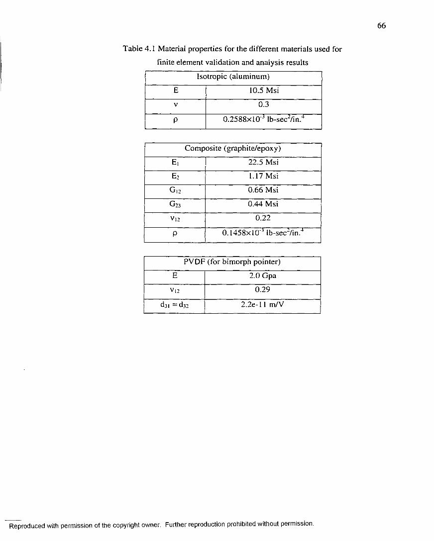
6 6
Table 4.1 Material properties for the different materials used for
finite element validation and analysis results
Isotropic (aluminum)
E 10.5 Msi
V 0.3
P 0.2588x1 O'3 lb-sec2/in.4
Composite (graphite/epoxy)
H, 22.5 Msi
H: 1.17 Msi
G ,2 0.66 Msi
G23 0.44 Msi
V12 0.22
P 0.1458x10'3 lb-sec2/in.4
PVDF (for bimorph pointer)
E 2.0 Gpa
V12 0.29
d3l = d32 2.2e-l 1 m/V
Reproduced with permission of the copyright owner. Further reproduction prohibited without permission.

67
Table 4.2 Comparison between natural frequencies using MIN3 element
and using analytical solution for square isotropic panel
Mode (n , m )Frequency (Hz)
12x12 MIN3 Analytical
( 1, 1) 66.5482 66.4903
(2 , 1) 165.9355 166.2259
(2 ,2 ) 266.8552 265.9614
(3,1) 332.4625 332.4517
(3,2) 430.1436 432.1872
(3,3) 564.7975 565.1679
Table 4.3 Comparison of static deflection for the piezoelectric bimorph
beam (10‘7 m) using different methods (see Figure 4.2)
Position 1 2 3 4 5
Analytical [69] 0.138 0.552 1.242 2.208 3.450
Solid FE [78] 0.138 0.552 1.242 2.208 3.450
QUAD4 [77] 0.14 0.55 1.24 2.21 3.45
MIN3 0.149 0.587 1.289 2.256 3.487
Reproduced with permission of the copyright owner. Further reproduction prohibited without permission.
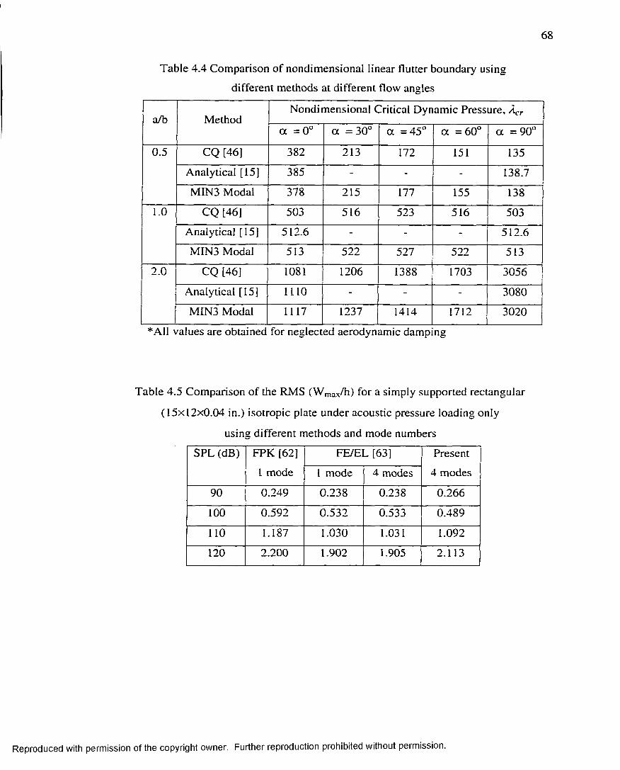
6 8
Table 4.4 Comparison of nondimensional linear flutter boundary using
different methods at different flow angles
a/b MethodNondimensional Critical Dynamic Pressure, A cr
ft II o 0 a = 30° a =45° a =60° a =90°
0.5 CQ [46] 382 213 172 151 135
Analytical [15] 385 - - - 138.7
MIN3 Modal 378 215 177 155 138
1.0 CQ [46] 503 516 523 516 503
Analytical [15] 512.6 - - - 512.6
MIN3 Modal 513 522 527 522 513
2.0 CQ [46] 1081 1206 1388 1703 3056
Analytical [15] 1110 - - - 3080
MIN3 Modal 1117 1237 1414 1712 3020
*AI1 values are obtained for neglected aerodynamic damping
Table 4.5 Comparison of the RMS (W max/h) for a simply supported rectangular
(15x12x0.04 in.) isotropic plate under acoustic pressure loading only
using different methods and mode numbers
SPL (dB) FPK [62]
1 mode
FE/EL [63] Present
4 modesI mode 4 modes
90 0.249 0.238 0.238 0.266
100 0.592 0.532 0.533 0.489
110 1.187 1.030 1.031 1.092
120 2.200 1.902 1.905 2.113
Reproduced with permission of the copyright owner. Further reproduction prohibited without permission.
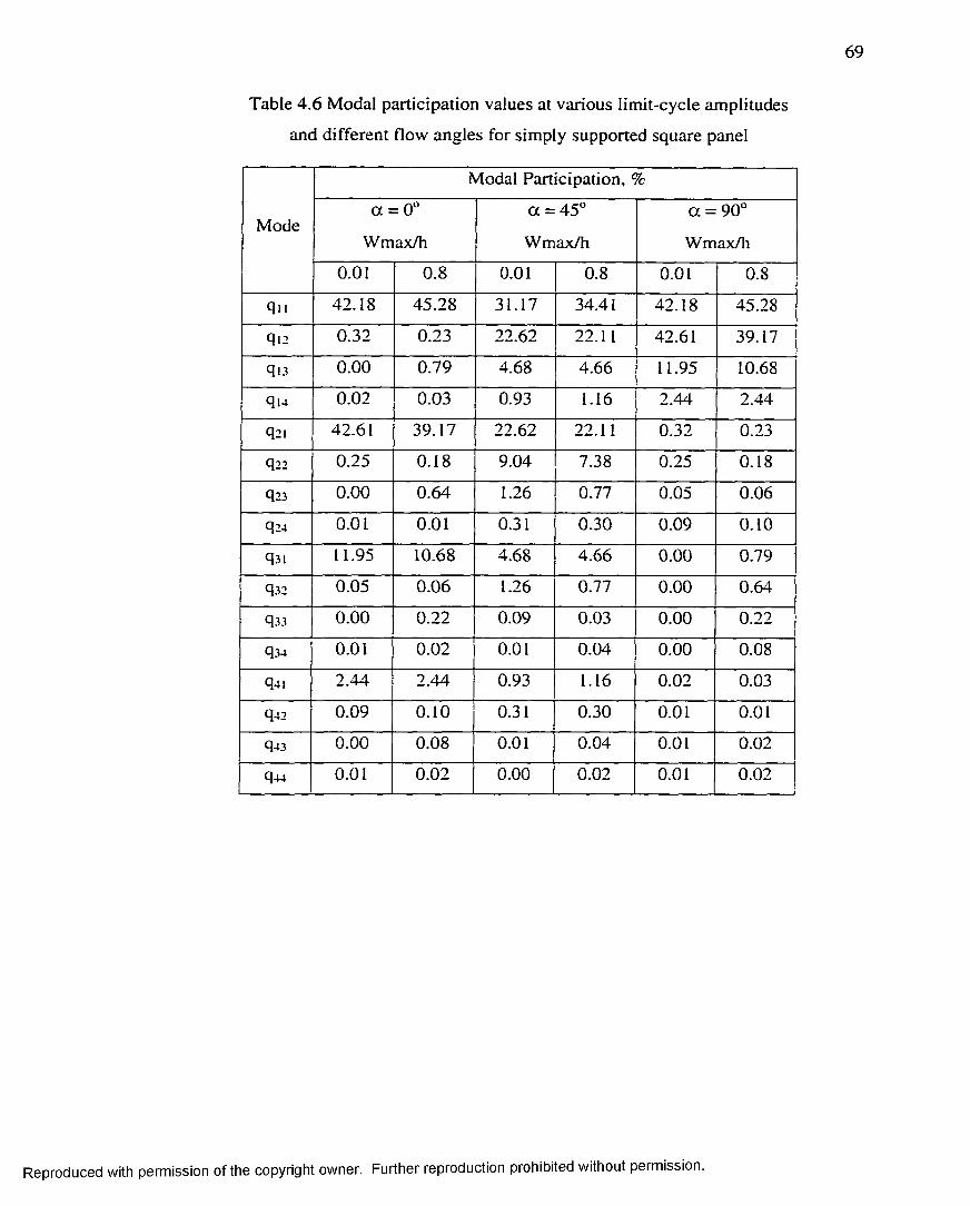
69
Table 4.6 Modal participation values at various limit-cycle amplitudes
and different flow angles for simply supported square panel
Mode
Modal Participation, %
a = 0°
Wmax/h
a = 45°
Wmax/h
a = 90°
Wmax/h
0.01 0.8 0.01 0.8 0.01 0.8
qu 42.18 45.28 31.17 34.41 42.18 45.28
qi2 0.32 0.23 22.62 22.11 42.61 39.17
qi3 0.00 0.79 4.68 4.66 11.95 10.68
q u 0.02 0.03 0.93 1.16 2.44 2.44
q2i 42.61 39.17 22.62 22.11 0.32 0.23
q22 0.25 0.18 9.04 7.38 0.25 0.18
q23 0.00 0.64 1.26 0.77 0.05 0.06
q24 0.01 0.01 0.31 0.30 0.09 0.10
q3i 11.95 10.68 4.68 4.66 0.00 0.79
q32 0.05 0.06 1.26 0.77 0.00 0.64
q33 0.00 0.22 0.09 0.03 0.00 0.22
q34 0.01 0.02 0.01 0.04 0.00 0.08
q4i 2.44 2.44 0.93 1.16 0.02 0.03
q42 0.09 0.10 0.31 0.30 0.01 0.01
q43 0.00 0.08 0.01 0.04 0.01 0.02
q44 0.01 0.02 0.00 0.02 0.01 0.02
Reproduced with permission of the copyright owner. Further reproduction prohibited without permission.

70
Table 4.7 Modal participation values at various limit-cycle amplitudes and different flow
angles for simply supported rectangular graphite/epoxy [0/45/-45/90]s panel
Modal Participation, %
Modea == 0° a = 45° a =
oOO'Wmax/h Wmax/h Wmax/h
0.01 0.8 0.01 0.8 0.01 0.8
qi 24.85 29.87 22.74 25.24 25.62 27.43
qa 16.54 12.64 29.59 24.37 41.11 36.57
q3 31.92 33.52 17.47 21.17 3.61 4.04
q-t 5.58 3.45 5.22 4.65 7.19 6.38
qs 1.16 0.07 11.93 9.91 13.13 12.15
q6 15.37 15.03 3.35 5.74 0.12 1.65
q? 0.48 1.01 1.47 0.43 1.55 2.29
qs 0.68 0.21 0.92 0.83 0.28 0.78
q« 0.04 0.07 3.27 3.00 4.08 4.27
qio 0.01 0.18 0.07 0.04 0 .1 1 0.81
qn 3.10 3.38 0.77 1.60 0.01 0.00
qi2 0.02 0.07 0.36 0.01 0.20 0.10
qi3 0.16 0.09 0.39 0.61 0.01 0.01
qi4 0.00 0.06 2.21 2.00 2.89 2.88
qis 0.01 0.09 0.01 0.03 0.01 0.52
qi6 0.00 0.17 0.16 0.30 0.00 0.05
Reproduced with permission of the copyright owner. Further reproduction prohibited without permission.

71
Table 4.8 Modal participation values at various limit-cycle amplitudes and different flow
angles for simply supported rectangular graphite/epoxy [-40/40/-40] panel
Mode
Modal Participation, %
a = 0°
Wmax/h
a = 45°
Wmax/h
a = 90°
Wmax/h
0.01 0.8 0 .0 1 0.8 0.01 0.8
qi 25.33 26.38 28.85 28.95 25.65 25.90
qa 41.18 35.26 44.90 40.35 39.10 32.55
q3 4.17 7.01 2.55 2.80 7.94 10.76
q4 11.38 9.79 12.06 11.55 9.87 8.67
qs 2.83 2.73 0.73 1.00 3.45 3.54
qe 6.15 6.75 6.15 7.25 4.52 5.25
q? 1.46 2.54 1.67 2.22 3.08 4.51
qs 2.32 2.13 0.18 0.27 2.10 2.13
qy 0.84 1.22 0.74 1.31 0.32 0.70
qio 1.05 1.55 0.89 1.61 1.06 1.58
qu 1.22 1.21 0.01 0.07 0.95 1.05
qi= 0.13 0.51 0.17 0.67 0.04 0.44
qi3 0.24 0.39 0.20 0.33 0.64 0.97
q u 0.74 1.17 0.65 1.22 0.64 1.01
qi5 0.83 1.02 0.09 0.00 0.42 0.74
q i6 0.07 0.26 0.07 0.32 0.15 0.13
Reproduced with permission of the copyright owner. Further reproduction prohibited without permission.

Table 4.9 Modal convergence for clamped rectangular [0/45/-45/90]s
graphite/epoxy panel at SPL = 120 dB and A = 800
Number of Modes RMS( Wmax/h)
1 0.5557
2 0.5845
6 0.7814
9 0.7798
16 0.8279
20 0.8110
25 0.8183
Selected 13 modes 0.8124
Table 4.10 Modal participation for a clamped rectangular [0/45/-45/90]s
graphite/epoxy panel at SPL = 120 dB and A = 800
Mode Participation, % Mode Participation, %
9i 36.72 914 4.19
92 5.24 915 0.38
93 19.3 916 0.99
94 4.25 917 1.38
95 4.01 918 2.55
96 7.67 919 0.21
97 1.71 920 0.27
98 0.76 921 0.53
99 0.33 922 0.33
9io 1.54 923 0.54
9u 4.77 924 0.14
912 0.35 925 1.54
913 0.28
Reproduced with permission of the copyright owner. Further reproduction prohibited without permission.

73
ik
b
k --------
Figure 4.1 Typical MIN3 elements mesh used to model rectangular and triangular panels
Reproduced with permission of the copyright owner. Further reproduction prohibited without permission.

74
Piezoelectric bi morph beam
I mm
mm0 cm
Clamped end
Figure 4.2 Clamped piezoelectric bimorph beam modeled using MIN3 elements
Reproduced with permission of the copyright owner. Further reproduction prohibited without permission.

Wm
ax/h
75
1
0.8
0.6
0.4
0.2 o M IN3 Frequency Domain — M IN3 Time Dom ain A— Analytical
o '—500 550 600 700650 750 800
Nondim ensional Dynamic Pressure
Figure 4.3 Validation of flutter limit-cycle amplitude for simply
supported square isotropic panel
Reproduced with permission of the copyright owner. Further reproduction prohibited without permission.

Wm
ax/h
76
0.8
0.6
0.4
0.2 • M IN3 Time Domains Rectangular Time Domain
280 300 320 340 360 380 400 420Nondimensional Dynamic Pressure
Figure 4.4 Validation of flutter limit-cycle amplitude for simply
supported square [0/45/-45/90]s laminate
Reproduced with permission of the copyright owner. Further reproduction prohibited without permission.

Wm
ax/h
77
1
0.8
0.6
0.4
0.2 12x 1210x 108 x8
e
o '—500 550 600 650 700 750 800
Nondimensional Dynamic Pressure
Figure 4.5 Finite element mesh convergence for simply supported
isotropic square panel at 45° flow angle and using 16 modes
Reproduced with permission of the copyright owner. Further reproduction prohibited without permission.

78
0.8
0.6■s2pm
£0.4
4 m odes 9 m odes 16 m odes 25 m odes6 m odes in x d irection
0.2
300 400 500 600 700 800 900Nondim ensional Dynamic Pressure
Figure 4.6 Modal convergence for simply supported isotropic
square panel at 0° flow angle
Reproduced with permission of the copyright owner. Further reproduction prohibited without permission.

Wm
ax/h
79
0.8
0.6
0.4
4 m odes 9 m odes 16 m odes 25 m odes
0.2
400 450 500 550 600 650 700 750 800Nondimensional Dynamic Pressure
Figure 4.7 Modal convergence for simply supported isotropic
square panel at 45° flow angle
Reproduced with permission of the copyright owner. Further reproduction prohibited without permission.

Wm
ax/h
8 0
0.8
0.6
0.4
0 degQ 15 deg
—©— 30 deg — 45 deg
0.2
500 550 600 650 700 750 800Nondimensional Dynamic Pressure
Figure 4.8 Effect of flow yaw angle on limit-cycle amplitude for
simply supported isotropic square panel
Reproduced with permission of the copyright owner. Further reproduction prohibited without permission.

81
0.8a /h = a /b = 2
0.6
I0.4
0.2
0 deg 45 deg
500 1000 1500 2000 2500Nondim ensional Dynamic Pressure
Figure 4.9 Effect o f panel aspect ratio at different yaw angles on limit-cycle amplitude
for simply supported isotropic panels
Reproduced with permission of the copyright owner. Further reproduction prohibited without permission.

8 2
0.5>-
0 0y (in.) x (in.)
?0.5-|
0 0y (in.) x (in.)
a = 45°
?o.sH
0 0y (in.) x (in.)
a = 90°
Figure 4.10 Flutter mode shape at different flow angles for
simply supported isotropic square panel
Reproduced with permission of the copyright owner. Further reproduction prohibited without permission.

83
0.8
0.6
0.4
■s— 4 modes -©— 9 modes 16 modes
25 modes
0.2
150 200 250 300 350 400 450Nondimensional Dynamic Pressure
Figure 4.11 Modal convergence for simply supported rectangular
graphite/epoxy [0/45/-45/90]s panel at 45° flow angle
Reproduced with permission of the copyright owner. Further reproduction prohibited without permission.

84
0.8
0.6. s*5?cs£
£0.4
0.2 0 deg 45 deg 90 deg
150 200 250 300 350 400 450Nondim ensional Dynamic Pressure
Figure 4.12 Effect of flow yaw angle on limit-cycle amplitude for simply supported
rectangular graphite/epoxy [0/45/-45/90]s panel
Reproduced with permission of the copyright owner. Further reproduction prohibited without permission.
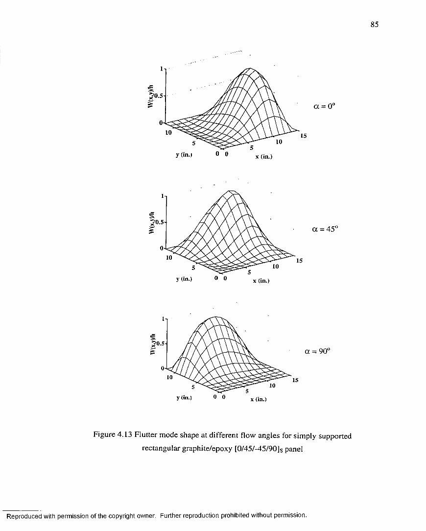
85
0 oy (in.) x (in.)
a = 0°
15
'0.5
0 0y (in.) x (in.)
a = 45°
15
0 0y (in.) x (in.)
a = 90°
15
Figure 4.13 Flutter mode shape at different flow angles for simply supported
rectangular graphite/epoxy [0/45/-45/90]s panel
Reproduced with permission of the copyright owner. Further reproduction prohibited without permission.

Wm
ax/h
8 6
0.8
0.6
0.4
4 m odes 9 modes 16 m odes 25 modes
0.2
A
100 120 140 160Nondim ensional Dynamic Pressure
180 2 2 02 0 0
Figure 4.14 Modal convergence for simply supported rectangular
graphite/epoxy [-40/40/-40] panel at 45° flow angle
Reproduced with permission of the copyright owner. Further reproduction prohibited without permission.

87
0 .8
0.6J5*5?csc
£0.4
0.2 0 deg 45 deg 90 deg
150 200 250 300Nondim ensional Dynamic Pressure
Figure 4.15 Effect of flow yaw angle on limit-cycle amplitude for simply supported
rectangular graphite/epoxy [-40/40/-40] panel
Reproduced with permission of the copyright owner. Further reproduction prohibited without permission.

8 8
0.5
0 0y (in.) x (in.)
a = 0°
15
0 0y (in.) x (in.)
1
§r^o.5
0
y ( ‘n-) 0 0 x (in.)
Figure 4.16 Flutter mode shape at different flow angles for simply supported
rectangular graphite/epoxy [40/-40/40] panel
Reproduced with permission of the copyright owner. Further reproduction prohibited without permission.

89
rA
0 .8
0.6
0.4
0.2 16 m odes 25 modes 36 modesA
3600 3800 4000 4200 4400 4600 4800 5000Nondimensional Dynamic Pressure
Figure 4.17 Modal convergence for simply supported triangular
isotropic panel at 45° flow angle
Reproduced with permission of the copyright owner. Further reproduction prohibited without permission.

Wm
ax/h
90
0.8
0.6
0.4
0 deg 180 deg 45 deg 225 deg 315 deg
0.2
30002500 3500 4000 4500 5000Nondimensional Dynamic Pressure
Figure 4.18 Effect of flow yaw angle on limit-cycle amplitude for
simply supported triangular isotropic panel
Reproduced with permission of the copyright owner. Further reproduction prohibited without permission.

(psi
)7H
z
-10
-12
500 1000 Frequency (Hz)
1500 2000
Figure 4.19 Power spectral density o f random input pressure at SPL = 90dB
Reproduced with permission of the copyright owner. Further reproduction prohibited without permission.

92
1.5
OdB 100 dB H O dB 120 dB
0.5
100 200 300 400 500 600 700 800Nondim ensional Dynamic Pressure
Figure 4.20 RMS of maximum deflection for simply supported square isotropic panel
under combined acoustic and aerodynamic pressures
Reproduced with permission of the copyright owner. Further reproduction prohibited without permission.

93
0.6
0.4
0.2
-0.4
- 0.6
- 0.80.1 0.2 0J 0.4
Time (Sec)
20
2-40
-60
-80200 400 600
Frequency (Hz)800 1000 1200
Figure 4.21 Time and frequency response for simply supported square
isotropic panel at SPL = 100 dB and X = 0
Reproduced with permission of the copyright owner. Further reproduction prohibited without permission.

>■
0.1 0.2 0_3 0.4Time (Sec)
20
-30
-40
-50 •
-60200 400 800600
Frequency (Hz)1000 1200
Figure 4.22 Time and frequency response for simply supported square
isotropic panel at SPL = 120 dB and X = 0
Reproduced with permission of the copyright owner. Further reproduction prohibited without permission.

-1.51---------------- '---------------- >--------------------------------0.42 0.44 0.46 0.48 0.5
Time (Sec)
40
20
-40
-60
-80
-100500 1000
Frequency (Hz)1500 2000
Figure 4.23 Time and frequency response for simply supported square
isotropic panel at SPL = 0 dB and X = 800
Reproduced with permission of the copyright owner. Further reproduction prohibited without permission.
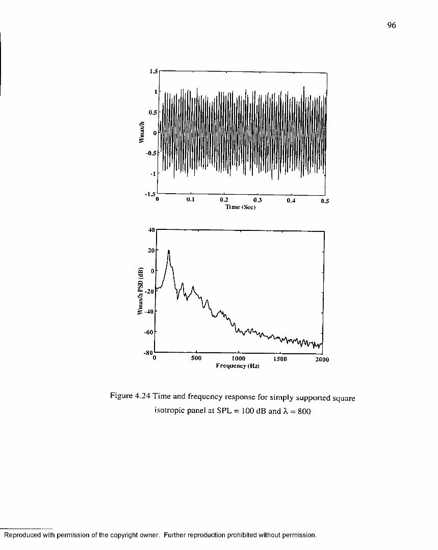
96
■»ss5£
0.1 03 0.4Time (Sec)
40
-20
> -40
-60
-80500 1000 1500 2000
Frequency (Hz)
Figure 4.24 Time and frequency response for simply supported square
isotropic panel at SPL = 100 dB and X = 800
Reproduced with permission of the copyright owner. Further reproduction prohibited without permission.

97
0.1 0 .2 0 .3Time (Sec)
20
> -40
-60
-80500 1000
Frequency (Hz)1500 2000
igure 4.25 Time and frequency response for simply supported square
isotropic panel at SPL = 120 dB and A. = 800
Reproduced with permission of the copyright owner. Further reproduction prohibited without permission.
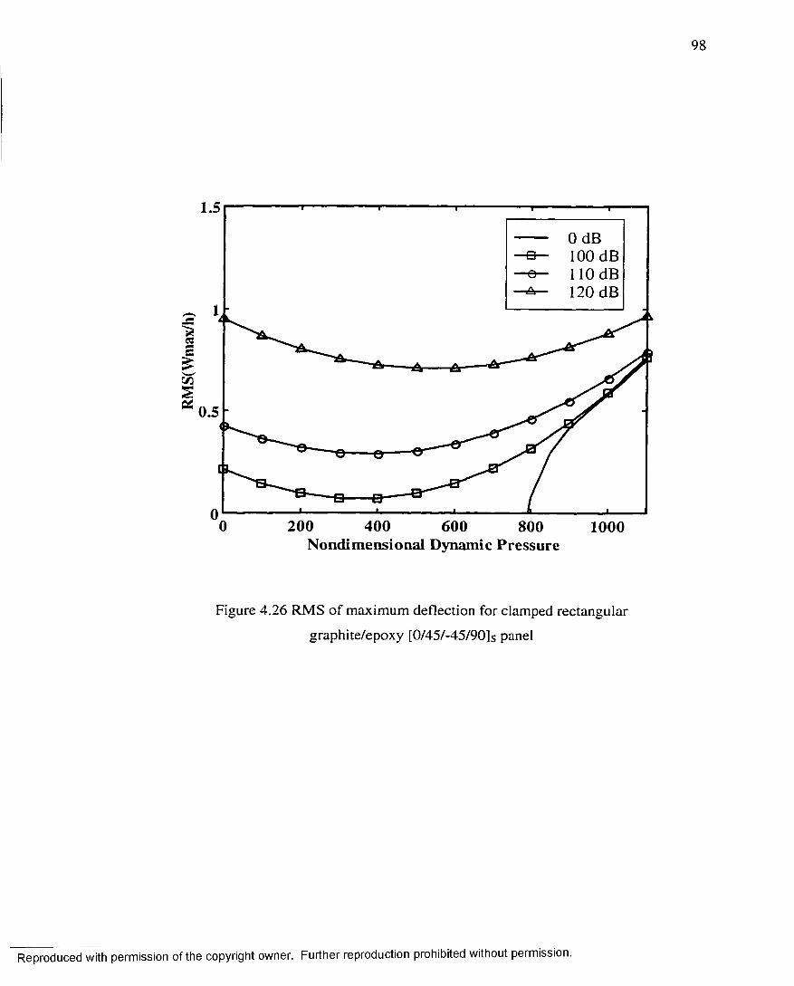
RM
S(W
max
/h)
98
1.5
0 dB 100 dB 110 dB 120 dB•& r
0.5
200 400 600 800Nondim ensional Dynamic Pressure
1000
Figure 4.26 RMS of maximum deflection for clamped rectangular
graphite/epoxy [0/45/-45/90]s panel
Reproduced with permission of the copyright owner. Further reproduction prohibited without permission.

99
CHAPTER V
CONTROL METHODS AND OPTIMAL PLACEMENT OF
PIEZOELECTRIC SENSORS AND ACTUATORS
5.1 Introduction
Many control strategies such as classical, optimal, Ho*, nonlinear, fuzzy logic, and
adaptive control have been utilized for vibration control in the literature. Two major
properties, the nonlinearity and the large dimension of the model, can characterize the
nature o f the problem of nonlinear panel flutter with yawed supersonic flow. Modem
control techniques such as optimal control and H,*, are very suitable for such systems, as
they can easily handle large dimension and no prior knowledge of the controller structure
is required.
In this study, optimal control strategies are the main focus for the suppression of
nonlinear panel flutter. The linear quadratic Gaussian (LQG) control, which combines
both linear quadratic regulator (LQR) optimal feedback and Kalman filter state estimator,
is considered as systematic linear dynamic compensator. To address the issue of the
flutter nonlinear dynamics involved, an extended Kalman filter for nonlinear systems is
also considered and combined with optimal feedback to form a nonlinear dynamic
compensator. Finally, a more practical approach based on optimal output feedback is
used to alleviate the problem of state estimation. Closed loop criteria based on the norm
of feedback control gains for actuators and on the norm of Kalman filter gains for sensors
are used to determine the optimal location of self-sensing piezoelectric actuators.
5.2 State Space Representation
For control design and simulation, the nonlinear modal equations of motion given
in Chapter 3, equations (3.15) and (3.16), need to be cast in the standard state space form.
In state space representation, the system equations o f motion are written in the form of
coupled first order differential equations. State space models provide a standard and
efficient representation of systems with large number o f DOF and of multi-input multi
output (MIMO) systems in the time domain. Linearization about reference equilibrium
points can be used to obtain a linear state space models that could be used for the design
Reproduced with permission of the copyright owner. Further reproduction prohibited without permission.

100
of modern optimal and robust control laws. The system states, AT, are defined as the panel
modal deflections and modal velocities:
X = (5.1)
The control input, U, and sensor output, Y, are the self-sensing piezoelectric actuators
input voltage and sensor charge output, respectively:
< / = K ) r = (5.2)
Thus, the system modal equations o f motion in the continuous time domain state space
form are:
X =(A + J A q ) x + BU
Y = CX + DU
where the system matrices are given by:
[0 ] [/]. - ^ K r 1^ ] -coi[Mbr ic d\
[o] [or-col[Mb l {i K q }+[Kqq]j [0]
(5.3)
[ A ] =
U a q ] = (5.4)
[B] =_[0] _ '
- co l [Mb l l [Kb(p] * [ c M k J [0]], [Z>] = [0]
The modal damping matrix [c^ ] contains both modal aerodynamic and modal structural
damping terms. The system matrix [ A A q ] represents the effect of nonlinear stiffness
matrices of the panel. By using linearization about the system reference point (point with
no deflection, {<7} = 0 ), the nonlinear system matrix vanishes and the state space model in
(5.3) reduces to a linear state space model given by:
X = AX + B U Y - C X + D U
If the sensor electrical circuit is set up to measure the time rate of electrical charge
(current) instead of the electrical charge, then the output matrix C is:
[C ]= [[0 ] [ / ^ ] ] (5.6)
Reproduced with permission of the copyright owner. Further reproduction prohibited without permission.

101
It has to be noted that for non-ideal self-sensing piezoelectric actuators, i.e., with no
perfect compensation for the piezoelectric capacitance term, the D matrix will be nonzero
and will contain the residual feedforward effect resulting from imperfect compensation.
As discussed in chapter 2, this effect is usually small and hence neglected in this study.
5.3 Control Methods
5.3.1 Linear Quadratic Regulator (LQR)
One of the most commonly used methods to design full state feedback control for
linear systems is the LQR which seeks a solution for the linear full state feedback
problem defined as:
U = - K X (5.7)
that minimizes a quadratic performance index, / , that is function of both system states
and control effort.
J = ° ] [ x T Q X + U T R u ] d t (5.8)0
where Q is a symmetric positive semi-definite state weighting and R is a symmetric
positive definite control effort weighting. The solution for the controller gains that
minimize the performance index of equation (5.8) for the linear state space system give
by equation (5.5) is:
K = R ~ 1 B T P (5.9)
where P is a positive definite symmetric matrix determined from the solution of the
Riccati equation defined as:
P = A T P + P A - P B R ~ 1 B T P + Q (5.10)
In general, the optimal feedback gain sequence is time varying. For linear time invariant
systems, the value o f the optimal gain converges very quickly to a fixed value. The final
fixed value gain could be used as a suboptimal solution since it is easier for
implementation. For the case of fixed gain suboptimal feedback gain, the Riccati equation
reduces to the well know algebraic Riccati equation (ARE):
A 7 P + P A - P B R ~ 1 B T P + Q = 0 (5.11)
Reproduced with permission of the copyright owner. Further reproduction prohibited without permission.

1 0 2
The weighting matrices Q and R are used as control design tuning parameters. The
selection of Q and R requires some trials to achieve certain system response
characteristics.
5.3.2 Optimal Linear State Estimation
The application of LQR is not feasible in most cases because it is difficult to have
sensors that measure all system states. In addition, sensor outputs are usually noisy and
the system dynamics is not known exactly. One solution to this problem is the use of
probabilistic approach for both process dynamics and sensor noise. This leads to the well
known Kalman filter state estimator. Kalman filter is a set of recursive mathematical
equations that provide a solution to the least squares optimal state estimation problem in
the presence of process and sensor noise.
Consider a standard linear state space model as the one given in equation (5.5)
with added process and sensor noise:
where rj and v are uncorrelated process and measurement Gaussian white noise with zero
mean and known covariance matrices, Q e = E { r j r f } and R e = E{vvr }. Kalman filter
achieves optimal state estimation by minimizing the covariance matrix o f state estimation
error defined as:
leads to the standard linear Kalman filter estimator described by the following dynamic
equations:
In these equations, the error covariance matrix, Pe, and the estimator gain, Ke, are time
varying quantities. For the special case of linear time invariant systems with time
invariant process and sensor noise, the error covariance time derivative converges very
quickly to zero; hence, the Kalman filter gains become a constant matrix. For this case.
X = A X + B U + n Y = C X + D U + V
(5.12)
(5.13)
where X is the estimated state vector. The minimization of the error covariance matrix
X = A X + B U + K e ( Y - C X )
Pe = A P e + P e A T - P eC T R ; 1CPe + Q e
K e = PeC T R g 1
(5.14)
Reproduced with permission of the copyright owner. Further reproduction prohibited without permission.

103
the error covariance matrix is determined using the solution of the estimator algebraic
Riccati equation (ARE) given by:
A P e + P e A T - P e C T R ~ l C P e + Q e = 0 (5.15)
As for the case of LQR, some tuning is required to select R e and Q e in order to achieve
good filter performance.
5.3.3 Linear Quadratic Gaussian Controller (LQG)
LQR and Kalman filter can be combined together to form the more practical
controller referred to LQG compensator shown in Figure (5.1). In LQG, the controller
output is based on the estimated states instead of the actual states:
U = - K X (5.16)
The LQG controller is based on the linear systems separation principle that allows
separate design of a feedback control gain and of an observer gain to form a dynamic
compensator. Since the Kalman filter is a dynamic system, the LQG is then a linear
dynamic regulator of the same kind used in classical control theory. However, unlike
classical control, the design of LQG is systematic and does not require any knowledge of
the controller structure. This makes LQG very suitable for designing stable control
systems for high order MIMO systems such as the application at hand, nonlinear panel
flutter suppression.
One popular method to design robust LQG compensator is to use the loop-transfer
recovery technique (LQG/LTR). This technique is based on recovering the guaranteed
robustness properties of the LQR (infinite gain margin and 60 degrees phase margin) to
the corresponding LQG controller. This can be achieved by tuning the LQG Kalman filter
weighting matrices Q e and R e to asymptotically recover LQR loop transfer function. One
way to select the Kalman filter weighting is:
R e = m > Q e = v 2 B B T (5.17)
As v goes to infinity, the loop transfer function of LQG controller approaches the loop
transfer function of LQR. However, the value of v should not be increased indefinitely as
this leads to very high Kalman gains. The LQG/LTR is a frequency domain loop shaping
approach that could be used to satisfy specific robustness bounds on the open loop
transfer function.
Reproduced with permission of the copyright owner. Further reproduction prohibited without permission.

104
5.3.4 Extended Kalman Filter (EKF)
One major drawback with the application of linear Kalman filter to the problem of
nonlinear panel flutter suppression is that it assumes linearized system equations about
the reference no deflection point. Hence, the nonlinear effects are not considered at all in
the estimation process. As it will be shown in Chapter 6 , this could deteriorate the state
estimation performance for large limit cycle amplitudes. One solution to such a problem
is to use Kalman filter that performs the linearization about a trajectory that is
continuously updated with the estimated states. Such filter is referred to as extended
Kalman filter (EKF) [109], The equations of an EKF for the nonlinear state space model
o f panel flutter, equation (5.3), are given by:
X = A X + BU + K e (Y —CX)
Pe = A P e + Pe A T — PeC T R ~ l CPe + Q e6 e e e v e ( 5 [ g )
K e = P eC T R ; 7
A = A + AAq (X)
where the term AAq (X) represents the nonlinear state space matrix evaluated using the
current state estimate. Unlike the standard Kalman filter, the EKF gain sequence cannot
be predetermined and has to be evaluated on-line. This adds more computational cost but
should not be a problem especially with the advanced and fast real time processors
available today. The EKF deviates from the standard linear Kalman filter because of the
nonlinear feedback of the measurement into the system model and because the various
random variables are no longer Gaussian after undergoing nonlinear transformation.
Thus, the EKF is simply an ad hoc state estimator for nonlinear systems. However, it has
proven to be successful in various applications [109-112],
5.3.5 Nonlinear Controller using EKF and LQR
The EKF can be combined with LQR to form a nonlinear dynamic output
compensator for the control o f nonlinear panel flutter, see Figure (5.2). Such controller is
nonlinear because the estimated state and consequently the control effort, U, is a dynamic
nonlinear function of the measured sensor output. The advantage of this controller over
the LQG controller is the more accurate state estimation for the nonlinear panel flutter
dynamics.
Reproduced with permission of the copyright owner. Further reproduction prohibited without permission.

105
5.3.6 Optimal Output Feedback Control
A simpler control strategy for MIMO systems that avoid the need for state
estimation is to design an output feedback compensator of the form:
The output feedback gain matrix, Ky, can be determined using optimal control by
minimizing the quadratic performance index given in equation (5.8). However, this leads
to a feedback control gain that is dependent on the states initial conditions which is
undesirable. This problem can be avoided by minimizing the expected value of the
performance index, E{J}\ hence, the minimization is performed over a distribution of
possible values for the initial conditions. The design equations for optimal output
feedback control are given by [108]:
The expected initial state is usually assumed uniformly distributed on the unit sphere in
order to drive any initial state to zero. It can be seen from equation (5.20) that the
solution for the optimal output feedback gain requires a solution of three coupled
nonlinear algebraic matrix equations. These equations can be solved using the gradient-
based iterative method described in Appendix C [108].
The method adopted for actuator placement in this study is the method of norm of
optimal feedback control gain matrix (NFCG) used for panel flutter suppression by [74]
and [100]. This method determines the effectiveness o f a piezoelectric actuator by using
the norm o f feedback gain designed using LQR and thus is a closed loop criterion.
The higher the value of N F C G , the more effective is the actuator for panel flutter
suppression.
U = —K y Y (5.19)
a J p + PAc + C T K Ty R K y C + Q = 0
A c s + s a J + X o = 0K y = R ' 1 B T P S CT (CSCT )~l
(5.20)
where
A c = A - B K C , (5.21)
5.4 Optimal Placement of Piezoelectric Sensors and Actuators
NFCG = |^ ijQR | (5.22)
Reproduced with permission of the copyright owner. Further reproduction prohibited without permission.

106
The NFCG method is extended for optimal sensor location by using the norm of Kalman
filter estimator gain (NKFEG).
N K F E G = \\K Kaiman || (5 .23)
The higher the value of NKFEG, the more effective is the sensor for the problem of state
estimation.
For the problem of panel flutter suppression, a number o f piezoelectric patches
equal to the number of finite element mesh size are used. The effectiveness of each
element as an actuator and as a sensor is determined using the above two criteria. The
shape and location of optimal actuator and sensor is then determined by combining the
most effective elements. Although each piezoelectric patch might act as both actuator and
sensor (self-sensing actuators), the optimal location for actuator and sensor might not be
the same.
Reproduced with permission of the copyright owner. Further reproduction prohibited without permission.

107
LQG
U = - K XLQR
System
Kalman Filter
Figure 5.1 Block diagram representation of the LQG controller
Reproduced with permission of the copyright owner. Further reproduction prohibited without permission.

108
Nonlinear Dynamic Controller
U = - K X
LQR
NonlinearSystem
Nonlinear State Estimator
(EKF)
Figure 5.2 Nonlinear dynamic compensator for nonlinear
panel flutter suppression using EKF and LQR
Reproduced with permission of the copyright owner. Further reproduction prohibited without permission.

109
CHAPTER VI
NONLINEAR PANEL FLUTTER SUPPRESSION RESULTS
6.1 Introduction
Simulation studies for the suppression of nonlinear panel flutter using
piezoelectric material under yawed supersonic flow are presented in this chapter. The
time domain nonlinear finite element modal equations of motion are used to simulate the
panel nonlinear flutter using the Runge-Kutta integration method. The studies presented
have two main objectives. The first objective is the comparison of the controllers
presented in Chapter 5 to determine the effect of different control strategies on the panel
flutter suppression performance. The closed loop system performance is also studied
under system parameter variations. This detailed controller performance study is
performed for the case of zero flow yaw angle. The second objective is controlling
nonlinear panel flutter under yawed supersonic for a specific range of yaw angles (the
range selected in this study is from 0° to 90°).
Panel flutter suppression under yawed supersonic flow is considered for isotropic
square, composite rectangular graphite/epoxy, and isotropic triangular panels. The
properties for both isotropic and composite materials were given in Table 4.1. The main
piezoelectric ceramic used in this study is the isotropic PZT5A. The mechanical and
electrical material properties of PZT5A are given in Table 6.1. The piezoelectric layers
are embedded on the top and bottom layers o f the panel to avoid disturbing the flow filed
over the panel. Each piezoelectric layer will be used as either self-sensing actuator or as
actuator only.
6.2 Square Isotropic Panel
A square simply supported isotropic panel (12x12x0.05 in.) is first used to study
different control methods and to study the control of panel flutter under a range of flow
yaw angles. Piezoelectric layers are embedded on the top and bottom surfaces of the
panel. The piezoelectric thickness is selected as 0.01 in. compared to the panel total
thickness of 0.05 in. Using this thickness, the actuation voltage is then limited to 152
Reproduced with permission of the copyright owner. Further reproduction prohibited without permission.

110
Volts (see Table 6.1). The aerodynamic damping coefficient, c a , is assumed 0.01 and a
structural modal damping ratio of 1% is added for all modes.
The panel is modeled using 10x10 finite element mesh and the nonlinear modal
equations of motion are derived using a selected number of modes based on modal
participation and modal convergence. For the case of zero flow yaw angle, four modes in
the flow direction, mode (1,1) to (4,1), are used for modal reduction. This allows for a
low order open loop system and, also, provides reasonably good accuracy for the flutter
limit-cycle oscillation (LCO) amplitude (see modal participation values at a = 0° in Table
4.6). This low order model is used for the detailed controller performance study. For the
case of arbitrary yaw angle, the panel nonlinear modal equations of motion are derived
using 16-mode model, mode (1,1) to (4,4). This makes the state space system of order 32.
6.2.1 Optimal Placement of Self-Sensing Piezoelectric Actuators
The first step is determining the optimal location of the embedded piezoelectric
layers to achieve optimal actuation and optimal sensing. The panel is divided into 10x10
mesh size and is completely covered on top and bottom with piezoelectric layers (total of
100 piezoelectric actuators/sensors). The modal equations of motion are derived using the
16-mode model in order to be able to determine the optimal actuator and sensor locations
for different yaw angles. The linearized system equations of motion about the zero
displacement point, equation (5.5), are used to design both optimal feedback control
(LQR) and optimal observer (Kalman filter). The resulting optimal feedback gain, K , and
observer gain, K e, are matrices with sizes 100x32 and 32x10, respectively. They
represent the feedback and the estimator gain vectors for each patch of the 100
piezoelectric patches used. The methods of NFCG and NKFEG are then used to
determine the effectiveness of each piezoelectric patch for optimal actuation and sensing.
Figures 6.1 and 6.2 show contours of the values of NFCG and NKFEG for the
cases of 0° and 45° flow yaw angles, respectively (A is set to 1000 for this case). These
figures show clearly how the optimal actuator and sensor locations change completely for
different flow angles. This indicates the importance of considering the flow yaw angle
effect for the problem of panel flutter suppression. It is also seen that the optimal sensor
location is at the trailing edge (TE), where the maximum panel deflection point is located,
while the optimal actuator location is at the panel leading edge (LE) in the flow direction.
Reproduced with permission of the copyright owner. Further reproduction prohibited without permission.

I l l
The optimal sensor location agrees with the standard structural vibration applications by
placing the sensors at the maximum deflection point which gives minimum noise to
signal ration. However, the optimal actuator location doesn’t agree with the placement
guidelines that are well known for structural vibration, which usually places piezoelectric
actuators at the maximum curvature or maximum strain location. This is due to the
aerodynamic loading involved in the panel flutter problem, which is proportional to the
transverse deflection slopes (vvr and wv). Thus for A > A cr, considering the flutter
deflection shape shown in Figure 4.10, the panel is subjected to a distributed pressure
with maximum amplitude at the panel TE. It is found that the most effective piezoelectric
actuators to counteract this forcing aerodynamic pressure are those located at the panel
LE. This conclusion is in agreement with the experimental testing results performed by
[106],
Figures 6.3 and 6.4 show the selected piezoelectric actuator and sensor location
based on the NFCG and NKFEG methods for 0° and 45° yaw angles, respectively.
Rectangular shaped piezoelectric patches are used to obtain practical sensor and actuator
shapes. However, the optimal sensor and actuator shape can be refined by using more
elements or triangular patches. The optimal sizing of piezoelectric actuators is outside the
scope of this study and hence the size of both pieces is assumed by using the most
effective 12 elements. This assumption is based on the studies performed by [74] which
showed that the optimal size of actuator is between 10% and 20% of the panel area for
nonlinear panel flutter suppression. Since self-sensing piezoelectric actuators are utilized
in this study, the size of both patches located at the LE (optimal actuator) and at the TE
(optimal sensor) is assumed to be the same, as both of them will be used as actuators. In
practice, other types of sensors may be used such as accelerometers, displacement
sensors, or strain gages. A case with single LE actuator and displacement sensors is
considered when designing optimal output feedback control law.
6.2.2 Controller Study
A study of the performance of different controllers described in Chapter 5 is
performed in this section. Two main categories o f controllers are used. The first category
is state feedback using LQR based on estimated states. Linear state estimation using
standard Kalman filter is considered which leads to the LQG controller. In addition.
Reproduced with permission of the copyright owner. Further reproduction prohibited without permission.

1 1 2
nonlinear state estimation using extended Kalman filter (EKF) is introduced. The second
category considered is the optimal output feedback control.
The performance of different controllers is compared using their ability to
suppress the panel nonlinear flutter. The measure used to asses performance is the
maximum flutter-free dynamic pressure, A m a x, defined as the maximum dynamic pressure
at which the control system can suppress the LCO of nonlinear panel flutter given the
limitation of the actuator maximum voltage (saturation). This quantity is governed by
controller performance, piezoelectric saturation voltage, and LCO amplitude. To obtain
conservative values for A max, the controller will be activated after the convergence of
LCO.
For the comparison performed in this section, the panel at 0° yaw angle with the
embedded PZT5A piezoelectric self-sensing actuators shown in Figure 6.3 is considered.
The panel is modeled using the 4-mode model (state space model is of 8 lh order). Figure
6.5 shows the change of panel frequencies as the nondimensional dynamic pressure, A ,
increases for the panel with no piezoelectric material and with piezoelectric material
added. It is seen how the addition of piezoelectric material decreases the panel stiffness
compared to the original panel. This occurs because the piezoelectric material has heavier
mass and slightly softer Young’s modulus. Figure 6.6 shows the open loop poles at 3
different values of A . It is seen how increasing A beyond A cr results in 2 unstable poles
(after mode (1,1) and (2,1) coalescence) and increasing it further results in 4 unstable
modes as the other two modes, (3,1) and (4,1), coalesce.
6.2.2.1 LQR Controller
First a full state feedback using LQR is designed for the linearized model
assuming all the states available. As discussed in Chapter 5, this is not a practical control
method unless it is combined with state estimation. The state-weighting matrix, Q , is
selected using the energy method and the control-weighting matrix, R , is selected as a
constant multiplied by the identity matrix.
K 0 .0 M
Different values of ra re tested until satisfactory performance is achieved using r = 1000.
Figure 6.7 shows the performance of the LQR control for nonlinear panel flutter
Q = R = r [ l ] (6 . 1)
Reproduced with permission of the copyright owner. Further reproduction prohibited without permission.

113
suppression at A = 1500. The controller is activated at t = 100 msec and it suppresses the
LCO using the two self-sensing actuators at LE and TE within few cycles. A „ iax using this
controller was found to be 1760 compared to 512 for the original panel and to 449 for the
panel with embedded piezoelectric material and with no control applied.
6.2.2.2 LQG Controller
A Kalman filter estimator is designed based on the system linearized equations of
motion. Many values are used for the design parameters Q e and R e to arrive at
satisfactory estimator performance. The performance of the Kalman filter estimation is
shown in Figures 6.8 and 6.9 for A = 1000 and 2000 respectively. It is seen how the
estimated LCO amplitude degrade as A increases. This is expected as the Kalman filter
uses a linear model that does not consider the nonlinear effects at all, so it is trying to
estimate a nonlinear process using a linear model. As A increases, the effect of
nonlinearity increases and hence the estimated LCO amplitude using Kalman filter is not
accurate. The design parameters of the Kalman filters are selected as: Q e = [/], R e =
[C][C]T.
Figure 6.10 shows that, unlike the LQR, the LQG controller cannot suppress the
flutter LCO at A = 1500. Comparing this figure to the LQR performance, shown in Figure
6.7, shows how the introduction of linear state estimation degrades the control system
performance. The achieved A m a x using LQG is 920 compared to 1760 using LQR control,
which is about 50% performance reduction due to linear state estimation. Figure 6.11
shows the performance of the LQG controller at the maximum flutter-free dynamic
pressure.
6.2.2.3 Nonlinear Output Controller (EKF+LQR)
An extended Kalman filter estimator (EKF), which takes into account the system
nonlinear dynamic by linearizing about the estimated state vector, is implemented using
the same parameters as those of a Kalman filter (Q e, R e ). The performance of state
estimation using EKF is shown in Figure 6.12 at A — 2000. Comparing this to Figure 6.9
shows how superior the performance of EKF is compared to the standard Kalman filter. It
has to be noted that, in practice, the estimation performance will be further degraded due
to sensor noise and system model uncertainty.
Reproduced with permission of the copyright owner. Further reproduction prohibited without permission.

114
Combing the EKF with LQR control results in a dynamic nonlinear compensator.
Figure 6.13 shows the performance of the EKF+LQR for nonlinear panel flutter
suppression at A = 1500. Using this controller, A m ax was found to be 1750. To show the
performance of EKF+LQR control even with uncertainty in the model nonlinear matrix
used by the EKF, the controller is used with +/-25% uncertainty in the system nonlinear
matrix, A A q , used in propagating the state estimate, see equation (5.16). Figure 6.14
shows that the flutter LCO can be successfully suppressed using the EKF+LQR
controller with +/-25% uncertainty in A A q . Therefore, using nonlinear state estimation
instead of the standard linear state estimation for the problem of nonlinear panel flutter
gives much better results even with some uncertainty in the nonlinear model matrix.
In all the controllers above, LQR, LQG, and EKF+LQR, the simulation results
indicated that the self-sensing piezoelectric patch at the TE is not as effective as the LE
patch from actuation point of view. However, the TE piezoelectric patch is acting as the
optimal sensor to achieve better state estimation. Without this sensor, i.e., if the LE
sensor is only used, the estimation performance will be degraded dramatically due to the
high noise to signal ratio for the LE sensor resulting from smaller displacement at this
location.
6.2.2.4 Optimal Output Feedback Controller
The iterative algorithm given in Appendix C is used to solve the coupled
nonlinear equations given by equation (5.20) for optimal output feedback gain matrix. An
initial stabilizing gain, K a , has to be first determined using some trail and error. The
weighting matrices Q and R are the same as for the LQR case. For the panel
configuration of 2 self-sensing piezoelectric actuators, the resulting output feedback gain
matrix is of size 2x2. Using this configuration, an output feedback gain was successfully
designed to suppress flutter LCO up to A m ax = 1000. Figure 6.15 shows the performance
o f the optimal output feedback controller at the maximum flutter-free dynamic pressure.
It is noticed that this controller introduces less damping to the system compared to the
full state feedback control. In practice, low pass filters have to be used to filter out the
feedback signals from the sensors. This could degrade the optimal feedback performance
even more.
Reproduced with permission of the copyright owner. Further reproduction prohibited without permission.

115
Another panel configuration that uses only the LE actuator and uses two
displacement sensors located at (a/2, a/2) and (3a/4, a/2) is considered. The output
feedback gain for this configuration is o f size 1x2. Figure 6.16 shows that the optimal
output feedback can suppress LCO up to A mclx = 1100 for this case.
In conclusion, the optimal output feedback performance for panel flutter
suppression is less than using EKF+LQR control. However, the optimal output feedback
is much simpler for practical implementation as it does not require the on-line adaptation
needed for EKF. The achieved values of A m ax for the different controllers used are
summarized in Table 6.2.
6.2.2.5 Controller Robustness
A study for the effect of system parameter variation on the performance of both
EKF+LQR and optimal output feedback controllers is given in this section. First with
regard to the dynamic pressure A , it was found that for LQR and optimal output feedback,
the feedback gain determined at A nw x suppresses LCO for all values of A < A m a x.
However, for accurate state estimation X needs to be known since the system model is a
function of A . Figure 6.17 shows the effect of +25% mismatch in A between design model
and reality (simulation model) for both LQR and EKF+LQR controllers when the
simulation model has A = 1200. It is seen how the performance of EKF+LQR is degraded
in this case, mainly due to inaccurate state estimation.
The second type of system parameter variation considered is in the panel stiffness.
In section 6 .2.2.3, it was shown that, the EKF+LQR controller has a satisfactory
performance with +/-25% uncertainty in the design model nonlinear stiffness matrix. In
this section a +/-25% variation in the modal linear stiffness is considered, which
corresponds to about +/-13% uncertainty in the panel natural frequencies. Figure 6.18
shows the effect of +/-25% variation in modal linear stiffness using EKF+LQR controller
at A — 1500. It is seen that the LCO cannot be suppressed with such system parameter
variation. The performance of EKF+LQR is degraded with parameter variations because
both the state estimation and the state feedback design are affected by the linear stiffness
variation. Figure 6.19 shows the same effect for the optimal output feedback controller at
A = 1100 (using the configuration of single LE actuator and 2 displacement sensors). The
Reproduced with permission of the copyright owner. Further reproduction prohibited without permission.

116
optimal output feedback controller is shown to be more robust to linear stiffness variation
than the EKF+LQR controller.
6.2.3 Panel Flutter Control with Yawed Flow
In this section, nonlinear panel flutter suppression with flow yaw angle is
considered. The nonlinear dynamic output compensator (EKF+LQR) is used in this study
as it provides the best performance. First, the flow yaw angle, a , is considered as simply
a perturbation that is not considered in the design at all, i.e., not considered in the
piezoelectric placement or in the controller design. Figure 6.20 shows the performance of
the controller designed for a = 0° when the actual flow is at a = 45° and A = 800. The
results clearly indicate that the flutter LCO cannot be suppressed for a = 45° using the
control system designed for a = 0° even at such low dynamic pressure. This shows that
flow yaw angle has to be considered in the design of active control systems for nonlinear
panel flutter suppression. Figure 6.21 shows the effect of flow angle on the optimal
location of self-sensing piezoelectric actuators for a = 0, 15, 30, 45, and 90° flow yaw
angles. The flow LE piezoelectric patch is the optimal actuator location d6etermined
using NFCG while the TE patch is the optimal sensor location determined using NKFEG.
It is seen how the change of flow angle has a major effect o f the optimal actuator and
sensor locations.
The objective is to design active control system including piezoelectric placement
for the panel knowing that the panel will be subjected to a specific range of flow yaw
angles. The range assumed in this study is from 0 to 90°. Performing optimization for
piezoelectric placement over a range of a is not a simple task. The methodology
proposed in this study is to optimize the piezoelectric sensor and actuator placement for
different angles within the specified range, as was shown in Figure 6.21, then group the
resulting optimal location together to find a single piezoelectric configuration that works
over the entire range of angles.
Figure 6.22 shows optimal actuator and sensor location that covers all the yaw
angles from 0 to 90°. The optimal actuator consists o f 2 LE piezoelectric pieces in the
directions normal to 0 and 90° while the optimal sensor consists o f 2 TE piezoelectric
pieces in the directions normal to 0 and 90°. As mentioned before, the piezoelectric
patches required for optimal sensing can be replaced by other types of sensor such as
Reproduced with permission of the copyright owner. Further reproduction prohibited without permission.

117
strain gages or can be smaller in size. However, since they will be used as actuators too,
piezoelectric patches o f the same size are used. Thus, the configuration o f Figure 6.22
results in an outer square covering 48% of the panel surface with embedded PZT5A. The
embedded piezoelectric is divided into 4 equal self-sensing actuators referred to as: OLE
and 90LE for the leading edge patches perpendicular to the 0 and 90° flow directions, and
OTE and 90TE for the trailing edge patches perpendicular to the 0 and 90° flow
directions. Examining this configuration further, it is seen that it does not only cover yaw
angles from 0 to 90° but due to the panel symmetry and the usage o f self-sensing
actuators, this configuration will cover all angles from 0 to 360°.
The performance of the EKF+LQR controller for nonlinear panel flutter
suppression with yawed flow is now considered. Three different configurations for
piezoelectric placement are considered for comparison. The first and second
configurations are simply using the optimal placement determined at a = 0° and 45°,
respectively, while the third configuration uses the optimized piezoelectric over the range
o f 0 to 90° with 4 self-sensing actuators, as was shown in Figure 6.22. Figure 6.23 shows
a comparison of the achieved A m ax using these 3 configurations for flow yaw angles
changing from 0 to 90°. It is seen that the piezoelectric optimized for 0° flow angle
provides acceptable performance up to a = 45° with A m axl A cr - 3.03 ( A c r = 512), but
A m a J A c r decreases to about 1.56 at a = 90° compared to 3.41 at a = 0°. Therefore, this
configuration is not a good candidate for yaw angles from 0 to 90°. However, it provides
acceptable performance from 0 to 45° and consequently from -4-5° to 45° due to the panel
symmetry. The second configuration, piezoelectric optimized for a = 45°, is shown to
provide good flutter suppression performance over the entire range yaw angles from 0 to
90°. The best performance is achieved at a = 45° with A m axl A cr = 3.71 while A rnax! A cr =
3.0 at a = 0° and 90°. The third configuration with 4 self-sensing piezoelectric actuators
is shown to provide the best performance of all configurations with a minimum of
A m a x /A c r = 3.52 over the entire range of yaw angles. However, the second configuration
uses only 24% covered panel compared to 48% for the third configuration. Figures 6.24
through 6.26 show the time history of maximum LCO and the control inputs to the four
self-sensing piezoelectric actuators using the EKF+LQR controller at A = 1500 for a =
Reproduced with permission of the copyright owner. Further reproduction prohibited without permission.

118
0°, 45°, and 90°, respectively. They clearly indicate the effectiveness of proposed
controller and piezoelectric configuration in suppressing nonlinear panel flutter at
different flow yaw angles.
6.3 Composite Panel
Nonlinear panel flutter suppression with yawed supersonic flow is also considered
for a rectangular (15x12x0.048 in.) simply supported graphite/epoxy [0/45/-45/90]s
panel. PZT5A actuators that have the thickness of 0.006 in. are embedded at the top and
bottom layers, i.e., replacing the 0° layer. The maximum actuator applied voltage is
limited to 91.2 Volts in this case. The panel is modeled using 10x10 MIN3 finite element
mesh and the nonlinear modal equations of motion are derived using the lowest 16
modes. The aerodynamic damping coefficient, c a, is assumed 0.01 and the modal
structural damping ratio = 1%.
Adding too much piezoelectric material for this case will largely change the panel
characteristics as it replaces the 0° layer and hence change the original panel directional
properties. In addition, PZT5A mass density is very high compared to graphite/epoxy
(about 5 times higher). To avoid adding too much piezoelectric material and changing the
panel characteristics, piezoelectric material is only used as actuator for this panel and
displacement sensors are used to provide output measurements for the estimation process.
Similar to the isotropic panel case, the optimal actuator location is determined by
dividing the panel into 10x 10 piezoelectric actuator elements at the top and bottom then
using LQR state feedback gain matrix from these actuators to select the elements with the
highest NFCG. Figure 6.27 shows optimal piezoelectric actuator using this method for a
— 0, 15, 30, 45, and 90° flow yaw angles at A. = 800. Considering a yaw angle range from
0 to 90°, the approximate shape of optimal piezoelectric actuator that cover all angles
within this range is shown in Figure 6.28. It is basically the union of all elements at
different angles shown in Figure 6.27. The piezoelectric actuator shown in Figure 6.27 is
divided into two separate actuators one perpendicular to the 0° flow direction and the
other to the 90° flow direction. Three displacement sensors are used at the locations of
(3a/4, b l 2), (3a/4, 3 b / 4 ) , and { a l l , 3b/4) corresponding to the approximate location of
maximum deflection for 0°, 45°, and 90° yaw angles, respectively.
Reproduced with permission of the copyright owner. Further reproduction prohibited without permission.
119
Like to the isotropic panel, the performance of the EKF+LQR controller for
nonlinear panel flutter suppression is studied using three different configurations for
piezoelectric actuator placement: the optimal actuator for the case o f a = 0°, the optimal
actuator for a = 45°, and the optimized actuator over the range of 0 to 90° with 2
independent actuators, as shown in Figure 6.28. Figure 6.29 shows a comparison of the
achieved A m ax using these 3 configurations for flow yaw angles changing from 0 to 90°.
The critical dynamic pressure changes largely with flow angle for the original panel with
no piezoelectric actuators added as was shown in Figure 4.12 ( A cr= 315, 250, and 185 for
flow angles o f 0°, 45°, and 90°, respectively). The conclusion drawn from this figure are
very similar to those of the isotropic panel case and are summarized as follows:
• The actuator optimized for 0° flow angle does not provide good flutter
suppression performance over the range of 0 to 90°. However, it is reasonably
good for yaw angles from -45 to 45°.
• The best performance over the flow angles range of [0,90°] is achieved using the
actuator optimized for this range with 2 LE actuators (OLE and 90LE).
• The actuator optimized for 45° angle provides reasonably good performance for
all angles from 0 to 90° and has the advantage of being half the size of the
actuator optimized for all angles from 0 to 90°.
Thus, the panel maximum flutter free dynamic pressure can be increased to a minimum
of 750 over all yaw angles from 0 to 90° using the actuator optimized for 45° or to a
minimum of 900 using the actuator optimized for all angles from 0 to 90°. This is
compared to the minimum flutter-free dynamic pressure of 185 occurring at a = 90° for
the original panel. Figures 6.30 through 6.32 show the time history of maximum LCO
and the control inputs to the two piezoelectric actuators using the EKF+LQR controller at
A = 900 and for a = 0°, 45°, and 90° respectively. It shows the effectiveness of proposed
controller and piezoelectric configuration in suppressing nonlinear panel flutter at
different flow yaw angles for composite panels.
6.4 Triangular Panel
The triangular (12x12x0.05 in.) clamped isotropic panel studied in Chapter 4 is
considered for nonlinear panel flutter suppression. PZT5A layers with a thickness of 0.01
Reproduced with permission of the copyright owner. Further reproduction prohibited without permission.

120
in. are used. The panel is modeled using 10x10 MIN3 finite element mesh and the
nonlinear modal equations of motion are derived using the lowest 16 modes. The flow
yaw angles range selected for this panel is between 90° and 180°. This range is selected
since it encompasses the worst case yaw angle where the flow is parallel to the tilted edge
(or= 135° or 315°), as was shown in Chapter 4.
The optimal actuator location is determined by dividing the panel into 100
triangular piezoelectric elements at the top and bottom then using the NFCG method.
Figure 6.33 shows optimal piezoelectric actuator location using this method for different
yaw angles between 90° and 180°. An approximate shape and location of a single
piezoelectric actuator for the flow range from 90° to 180° is determined by combining the
optimum actuators at different angles within this range of yaw angles as given in Figure
6.34. A single displacement sensor is used at (0.2a, 0.46). This sensor location is
determined based on the locations o f maximum panel deflection at different flow angles
which are (0.2a, 0.36), (0.2a, 0.46), and (0.2a, 0.56) for a = 90, 135, and 180°,
respectively.
The performance of the EKF+LQR controller for nonlinear panel flutter
suppression is given in Figure 6.35. The panel maximum flutter free dynamic pressure is
increased to a minimum of 6350 compared to a minimum of 2620 for the uncontrolled
panel. The piezoelectric material and active control system for this panel is not as
effective as the case of square isotropic panel (3.5 times increase in X cr for the square
isotropic panel versus only 2.4 increase for the triangular panel). This is mainly due to the
smaller size and clamped boundary conditions of the triangular panel, which make it
stiffen
6.5 Summary
Simulation studies for the suppression of nonlinear panel flutter using
piezoelectric materials and different optimal control strategies are presented in this
chapter. The control strategies considered include LQG controller, LQR combined with
extended Kalman filter (EKF), and optimal output feedback. The nonlinear dynamic
output compensator compromised of LQR and EKF results in a 3.5 times increase in the
critical dynamic pressure compared to only 1.8 times for the LQG controller. Using
optimal output feedback controller, the panel critical dynamic pressure was increased
Reproduced with permission of the copyright owner. Further reproduction prohibited without permission.

121
about 2 times. However, the optimal output feedback is much simpler for practical
implementation as it does not require the on-line adaptation needed for EKF. Suppression
of nonlinear panel flutter under yawed supersonic flow is considered using the LQR and
EKF nonlinear controller. The NFCG and NKFEG methods are used to determine the
optimal location of piezoelectric actuators and sensors, respectively. Optimal actuator and
sensor location for a range of flow yaw angles is determined by grouping the optimal
locations for different angles within the specified range. Using this method with four self
sensing actuators, the critical flutter boundary was increased 3.5 times over the entire
range of yaw angles from 0 to 360° for square isotropic panel. For a rectangular
graphite/epoxy composite panel, the critical flutter dynamic pressure is increased to a
minimum of 900 over all yaw angles from 0 to 90° compared to 185 for the original
uncontrolled panel. Results for a clamped triangular isotropic panel showed that the
critical flutter dynamic pressure can be increased about 2.5 times for a flow yaw angle
range from 90 to 180°.
Reproduced with permission of the copyright owner. Further reproduction prohibited without permission.

1 2 2
Table 6.1 Mechanical and electrical properties PZT5A piezoelectric ceramics
PZT5A
H, 9.9 Msi (69 Gpa)
e 2 9.9 Msi (69 Gpa)
G [2 3.82 Msi (26.3 Gpa)
g 23 3.82 Msi (26.3 Gpa)
d3i -6.73x10 'y in/V (-171X101- m/V)
d32 -6.73x10 v in/V (-171X101" m/V)
P 0.72x1 O'J lb-sec‘/in.4(7700 K g/m ’)
Vi2 0.31*
he Same as layer thickness
Emax 15240 V/in (600 V/mm)
* hc: Electrode spacing
Table 6.2 Comparison of different controllers performance
for nonlinear panel flutter suppression
Controller ■max
LQR 1760
LQG 920
EKF+LQR 1750
Optimal OFB 1000-1100
Reproduced with permission of the copyright owner. Further reproduction prohibited without permission.

123
0.8
0.6
0.4
0.2
0.2 0.60.4 0.8x/a
(a)
0.8
0.6
£0.4
0.2
0.2 0.60.4 0.8x/a
(b)
Figure 6.1 Contours of (a) NFCG and (b) NKFEG for simply
supported square isotropic panel at 0° flow angle
Reproduced with permission of the copyright owner. Further reproduction prohibited without permission.

124
0.8
0.6
0.4
0.2
0.2 0.4 0.6 0.8x/a
(a)
0.8
0.6
0.4
0.2
0.2 0.4 0.6 0.8x/a
(b)
Figure 6.2 Contours of (a) NFCG and (b) NKFEG for simply
supported square isotropic panel at 45° flow angle
Reproduced with permission of the copyright owner. Further reproduction prohibited without permission.

125
Optimal Actuator Optimal Sensor
Figure 6.3 Selected self-sensing piezoelectric actuators placement and size for optimal
actuation and optimal sensing on square isotropic panel at 0° flow angle
Reproduced with permission of the copyright owner. Further reproduction prohibited without permission.

126
Optimal Actuator Optimal Sensor
Figure 6.4 Self-sensing piezoelectric actuators placement and size for optimal actuation
and optimal sensing on square isotropic panel at 45° flow angle
Reproduced with permission of the copyright owner. Further reproduction prohibited without permission.

Freq
uenc
y (H
z)
127
600
500
400
300
2 0 0
100No Piezo With Piezo
0 500 15001000 2000D yn am ic P re ssu re
Figure 6.5 Variation of First 4 linear modes versus X for isotropic
panel with and without added piezoelectric material
Reproduced with permission of the copyright owner. Further reproduction prohibited without permission.

Imag
inar
y
128
X X = 0, + X = 1000, V X = 2000
40 0 0
3 0 0 0
2000
1000
1000
-he-2000
-3 0 0 0
-4 0 0 01 0 0 ' 1-----------------------1000 -500 0 500 1000
Real
Figure 6.6 Open loop poles for isotropic square panels with embedded piezoelectric
material at different values of nondimensional dynamic pressure
Reproduced with permission of the copyright owner. Further reproduction prohibited without permission.

2
1
0
1
2
80 90 100 110 120
a 100ci.GLE
't e
© uu
1-100
9080 100 110 120Time (msec)
Figure 6.7 Limit-cycle amplitude and control inputs time history
for square isotropic panel using LQR control at X = 1500
Reproduced with permission of the copyright owner. Further reproduction prohibited without permission.

Permission of the
1.5
0.5
£ -0.5
-1.5
-2.5
85n " « (m sec)
100
F i g u r e 6 . 8 CnmmPanson be,ween
c o a m p l i t u d e us/no amplitude and tan fi,te r« A = 1000
“ pyright owner F„Bh

131
I++
ActualEstimated
75 8070 85 90 95 100Time (msec)
Figure 6.9 Comparison between actual LCO amplitude and estimated
LCO amplitude using Kalman filter at X = 2000
Reproduced with permission of the copyright owner. Further reproduction prohibited without permission.

Con
trol
Inp
ut
132
-2 •
80 90 100 110 120 130 140 150
100
LE't e-100 ■
80 90 100 110 120 130 140 150Time (msec)
Figure 6 .10 Performance of LQG controller at X = 1500
Reproduced with permission of the copyright owner. Further reproduction prohibited without permission.

Con
trol
Inp
ut
133
2
I
0
1
280 100 120 140 160 180 2 0 0
100
£-100
80 100 120 140 160 180 200Time (m sec)
Figure 6.11 Performance of LQG controller at the maximum
suppressible dynamic pressure, Xmax = 920
Reproduced with permission of the copyright owner. Further reproduction prohibited without permission.

134
2.5ActualEstimated
1.5
0.5-c■ac
£0.5
-1.5
-2.590 92 94 96 98 100
Time (m sec)
Figure 6.12 Comparison between actual and estimated LCO amplitude
using extended Kalman filter at k = 2000
Reproduced with permission of the copyright owner. Further reproduction prohibited without permission.
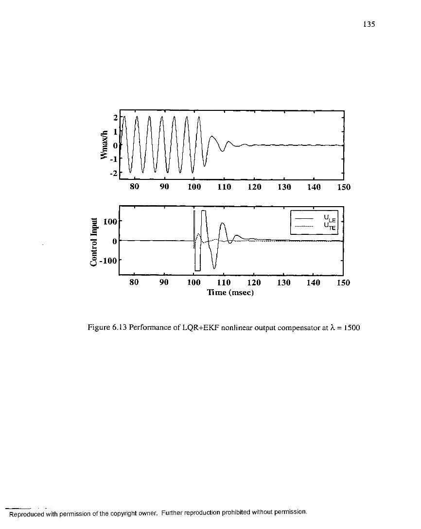
Con
trol
Inp
ut
135
2
1
0
1
2
80 90 100 110 120 130 140 150
£100
-100
80 90 100 110 120 130 140 150Time (msec)
Figure 6.13 Performance of LQR+EKF nonlinear output compensator at X = 1500
Reproduced with permission of the copyright owner. Further reproduction prohibited without permission.

136
21012
80 90 120100 1 1 0 130 140 150
LETE
1 00
0
- 1 0 0
80 90 120100 1301 1 0 140 150T i m e ( m s e c )
(a)
21012
80 90 100 1201 10 130 140 150
LETE
100a.s
- 1 0 0
80 90 120100 1 1 0 130 140 1 50T i m e ( m s e c )
(b)
Figure 6.14 Performance of LQR+EKF nonlinear output controller at X = 1500
with (a) -25% and (b) +25% uncertainty in the model nonlinear stiffness matrix
Reproduced with permission of the copyright owner. Further reproduction prohibited without permission.

Con
trol
Inp
ut
137
2
1
0
1
280 100 120 140 160 180 2 0 0
100
LE'TE
100
80 100 120 140 160 180 2 0 0Time (msec)
Figure 6.15 Performance of optimal output feedback controller
using two self-sensing actuators at Amax = 1000
Reproduced with permission of the copyright owner. Further reproduction prohibited without permission.

Con
trol
In
put
138
2
1
0
-1
280 100 120 180140 160 200
100
80 100 120 140 160 180 200Time (msec)
Figure 6.16 Performance of optimal output feedback controller using single
leading edge actuator and two displacement sensors at A.max = 1100
Reproduced with permission of the copyright owner. Further reproduction prohibited without permission.
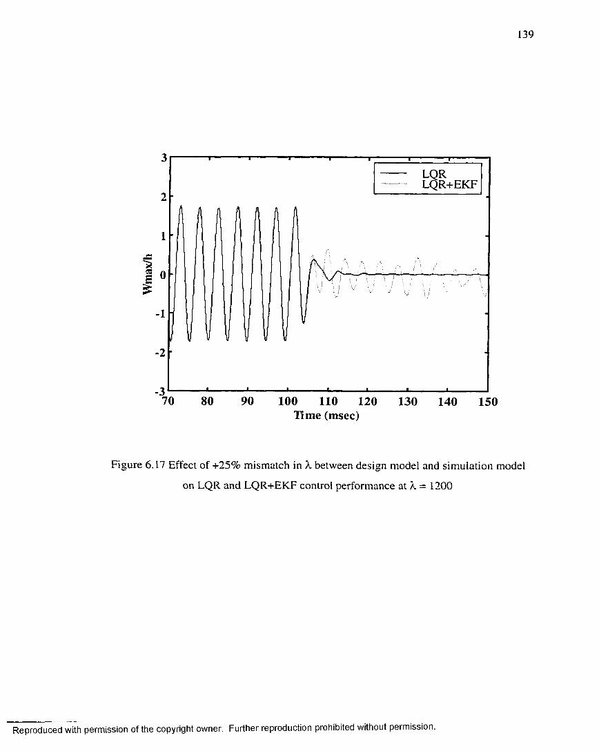
139
LQRLQR+EKF
csE
£
70 80 90 100 110 120 130 140 150lim e (msec)
Figure 6.17 Effect of +25% mismatch in X between design model and simulation model
on LQR and LQR+EKF control performance at X = 1200
Reproduced with permission of the copyright owner. Further reproduction prohibited without permission.

140
3
2
1
0
-1
-2
-3
80 100 120 140 160 180 200Time (msec)
Figure 6.18 Effect of design model linear stiffness variation on
The LQR+EKF controller performance at X = 1500
Reproduced with permission of the copyright owner. Further reproduction prohibited without permission.

+25%-25%1.5
0.5
E£
-0.5
-1.5
80 100 120 140 160 180 200l im e (msec)
Figure 6.19 Effect of design model linear stiffness variation on optimal
output feedback controller performance at X = 1100
Reproduced with permission of the copyright owner. Further reproduction prohibited without permission.

2
1
0
1
280 90 100 110 120 130 140 150
s 100
0
LE't e-100
80 90 100 120110 130 140 150Time (m sec)
Figure 6.20 Performance of EKF+LQR controller designed for
zero flow angle at X = 800 and 45 deg flow angle
Reproduced with permission of the copyright owner. Further reproduction prohibited without permission.

a = 0° a = 1 5 °
a = 45°
S i l l
a = 90°
Figure 6.21 Optimal actuator and sensor placement at different flow
angles from 0 to 90° for square isotropic panel
Reproduced with permission of the copyright owner. Further reproduction prohibited without permission.

144
Figure 6.22 Placement o f four self-sensing piezoelectric actuators for optimal actuation
and optimal sensing over the range of [0, 90°] flow angle for square isotropic panel
Reproduced with permission of the copyright owner. Further reproduction prohibited without permission.

145
2200
A.,max
1600
No PiezoPiezo optim ized for 0 deg Piezo optim ized for 45 deg Piezo optimized for [0-90] deg range
30 40 50 60Flow Yaw Angle (deg)
Figure 6.23 Comparison of panel flutter suppression performance using LQR+EKF
control at different flow yaw angles and using different piezoelectric placement
configurations for a square isotropic panel
Reproduced with permission of the copyright owner. Further reproduction prohibited without permission.

Con
trol
Inp
ut
Con
trol
In
put
146
2
0
280 90 100 110 120 130 140 150
100OLE'oTE
-100
80 90 100 110 120 130 140 150
10090LE'90TE
80 90 100 110 120 130 140 150Time (msec)
Figure 6.24 Performance of LQR+EfCF controller for square isotropic panel with 4 self
sensing piezoelectric actuators at 0° flow yaw angle and X = 1500
Reproduced with permission of the copyright owner. Further reproduction prohibited without permission.

Con
trol
In
put
Con
trol
Inp
ut
147
2
0
280 90 100 110 120 130 150140
100OLE'oTE
-100
80 90 100 110 120 130 140 150
10090LE'90TE
-100
80 90 100 110 120 130 140 150Time (msec)
Figure 6.25 Performance of LQR+EKF controller for square isotropic panel with 4 self
sensing piezoelectric actuators at 45° flow yaw angle and A. = 1500
Reproduced with permission of the copyright owner. Further reproduction prohibited without permission.

Con
trol
In
put
Con
trol
Inp
ut
148
2
0
280 90 100 110 120 130 140 150
100OLE'oTE
80 90 100 110 120 130 140 150
10090LE'90TE
9080 100 110 120 130 140 150Time (msec)
Figure 6.26 Performance of LQR+EKF controller for square isotropic panel with 4 self
sensing piezoelectric actuators at 90° flow yaw angle and A. = 1500
Reproduced with permission of the copyright owner. Further reproduction prohibited without permission.

149
a = 0 ° a = 1 5 °
a = 30° a = 45°
a = 90°
Figure 6.27 Optimal actuator placement at different flow angles
for [0/45/-45/90]s composite rectangular panel
Reproduced with permission of the copyright owner. Further reproduction prohibited without permission.

150
Figure 6.28 Optimal placement of 2 embedded piezoelectric actuators that cover
flow angles from 0° to 90° for [0/45/-45/90Js composite rectangular panel
Reproduced with permission of the copyright owner. Further reproduction prohibited without permission.

151
1600
1400
1200
100
-B-
'-max
0
No PiezoPiezo optim ized fo r 0 degPiezo optim ized fo r 45 degPiezo optim ized fo r [0,90] deg range
0 10 20 30 40 50 60F low Yaw Angle (deg)
70 80 90
Figure 6.29 Comparison of panel flutter suppression performance using LQR+EKF
control at different flow yaw angles and using different piezoelectric actuator
configurations for [0/45/-45/90]s rectangular composite panel
Reproduced with permission of the copyright owner. Further reproduction prohibited without permission.

Con
trol
Inp
ut
152
2
0
2
80 90 100 110 120 130 140 150
100
90
-50
-10080 90 100 110 120 130 140 150
Tim e (m sec)
Figure 6.30 Performance of LQR+EKF controller for rectangular
composite panel at 0° flow yaw angle and X = 900
Reproduced with permission of the copyright owner. Further reproduction prohibited without permission.

Con
trol
In
put
153
2
0
2
80 90 100 110 120 130 140 150
100
50 90
-50
-10080 90 100 110 120 130 140 150
Tim e (m sec)
Figure 6.31 Performance of LQR+EKF controller for rectangular
composite panel at 45° flow yaw angle and A = 900
Reproduced with permission of the copyright owner. Further reproduction prohibited without permission.

1
0.5
0
-0.5
180 90 100 110 130120 140 150
100
g, 50 90
.© -50
-10080 10090 110 120 140 150130
Tim e (m sec)
Figure 6.32 Performance of LQR+EKF controller for rectangular
composite panel at 90° flow yaw angle and k = 900
Reproduced with permission of the copyright owner. Further reproduction prohibited without permission.

155
t v\ \ V\ \ [x \\ \ \ \\ \ V \ \\ \ \ \\ \ \ \
a = 90°
a = 120°
a = 150°
a = 105°
a = 165°
a = 180°
Figure 6.33 Optimal actuator placement at different flow angles
for clamped triangular isotropic panel
Reproduced with permission of the copyright owner. Further reproduction prohibited without permission.

156
Figure 6.34 Optimal placement of a single self-sensing piezoelectric actuator that
approximately cover all angles from 90° to 180° for triangular clamped isotropic panel
Reproduced with permission of the copyright owner. Further reproduction prohibited without permission.
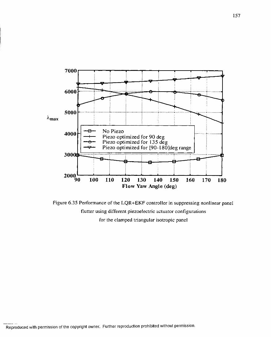
157
7000
6000
5000max
■H— No Piezo-i— Piezo optim ized for 90 deg •©— Piezo optim ized for 135 deg
Piezo optim ized for [90- I80]deg range
4000
300
200090
Flow Yaw Angle (deg)
Figure 6.35 Performance of the LQR+EKF controller in suppressing nonlinear panel
flutter using different piezoelectric actuator configurations
for the clamped triangular isotropic panel
Reproduced with permission of the copyright owner. Further reproduction prohibited without permission.

158
CHAPTER VII
SUMMARY AND CONCLUSIONS
A coupled structural-electrical modal finite element formulation for composite
panels, with integrated piezoelectric sensors and actuators, is presented and used to
analyze nonlinear supersonic panel flutter considering the effect of airflow yaw angle and
the effect o f additional high acoustic pressure loading. The finite element formulation is
also used for nonlinear panel flutter suppression with yawed airflow using optimal
control methods. The first-order shear deformation theory is used for laminated
composite panels and the von-Karman nonlinear strain-displacement relations are
employed for large deflection response. Structural-electrical coupling is considered using
the linear piezoelectricity constitutive relations. The first-order piston theory and
simulated Gaussian white noise are employed to model supersonic aerodynamic and
acoustic pressures, respectively. The coupled nonlinear equations of motion are derived
using the three-node triangular MIN3 plate element with improved transverse shear.
Additional electrical DOF per each piezoelectric layer is used to handle piezoelectric
sensors and actuators. Thus, the modified MIN3 element is a coupled structural-electrical
shear-deformable element for the nonlinear analysis o f smart composite structures. The
system equations of motion in the structure node DOF are transformed into the modal
coordinates using the panel linear vibration modes to obtain a set of nonlinear dynamic
modal equations o f lesser number. Modal participation is defined and used to determine
the number of modes required for accurate solutions. A new and efficient solution
procedure is presented using the LUM/LTF approximate method to solve the reduced
nonlinear modal equations for nonlinear panel flutter limit-cycle response. The presented
solution procedure has the advantage of using much less computational effort than
solving the system equations of motion in the structure node DOF.
The presented finite element modal formulation is validated by comparison with
other finite element and analytical solutions. Analysis results for the effect of arbitrary
flow yaw angle on nonlinear supersonic panel flutter for isotropic and composite panels
are presented using the modal LUM/NTF solution method. Results showed that the flow
Reproduced with permission of the copyright owner. Further reproduction prohibited without permission.
159
yaw angle completely changes the shape of the Iimit-cycle deflection. It also showed that
the effect of the yaw angle is a very important parameter especially for composite panels
where the flow direction may increase or decrease the nondimensional dynamic pressure
at Fixed limit-cycle amplitude depending on the panel lamination. The effect of combined
supersonic aerodynamic and acoustic pressure loading on the nonlinear dynamic response
of isotropic and composite panels is also presented. It is found that for panels at
supersonic flow, only acoustic pressure (sonic fatigue) is to be considered for low
dynamic pressures ( A « A cr ) and both acoustic and aerodynamic pressures must be
considered for significant and high aerodynamic pressures.
Simulation studies for the suppression of nonlinear panel flutter using
piezoelectric self-sensing actuators and using different optimal control strategies are
presented. The control strategies considered include LQG controller, LQR combined with
extended Kalman Filter (EKF) for nonlinear systems, and optimal output feedback. The
LQG controller performance was found to be much worse than the corresponding LQR
controller performance. This is mainly due to the use of linear Kalman filter to estimate
the states of nonlinear flutter dynamics. The state estimation is improved by using EKF.
The nonlinear dynamic output compensator compromised o f LQR control and EKF gives
much better performance for nonlinear panel flutter suppression with about 3.5 times
increase in the critical dynamic pressure compared to 1.8 times using LQG controller. By
using optimal output feedback controller the panel critical dynamic pressure was
increased about 2 times which is less than that of EKF+LQR controller. However, the
optimal output feedback is much simpler for practical implementation as it does not
require the on-line adaptation needed for EKF.
Nonlinear panel flutter suppression with airflow yaw angle is considered using the
EKF+LQR controller. Closed loop criteria based on the norm of feedback control gains
(NFCG) for actuators and on the norm of Kalman Filter estimator gains (NKFEG) for
sensors are used to determine the optimal location of self-sensing piezoelectric actuators
for different yaw angles. Optimal actuator and sensor location for a range of flow yaw
angles is determined by grouping the optimal locations for different angles within the
specified range. Using this method with four self-sensing actuators, the critical flutter
boundary was increased about 3.5 times over the entire range o f yaw angles from 0 to
Reproduced with permission of the copyright owner. Further reproduction prohibited without permission.

160
360° for square isotropic panel. For rectangular graphite/epoxy composite panel with two
actuators, the panel critical flutter dynamic pressure is increased to a minimum of 900
over all yaw angles from 0 to 90° compared to 185 for the original uncontrolled panel.
Results for a triangular isotropic panel with clamped boundaries showed that the critical
flutter dynamic pressure can be increased about 2.5 times for a flow yaw angle range
from 90 to 180° using the same methodology with a single piezoelectric actuator.
The main contributions of this research can be summarized as follows:
• Analysis o f nonlinear panel flutter of composite panels with yawed supersonic
flow using finite element method.
• Analysis of nonlinear composite panels response under combined aerodynamic
and high acoustic pressure loading.
• The consideration of state estimation problem for nonlinear panel flutter
suppression and the use of nonlinear state estimation based on EKF for improved
controller performance.
• Nonlinear flutter suppression o f isotropic and composite panels with yawed
supersonic flow.
Other minor contributions include, the derivation of coupled structural-electrical
nonlinear MIN3 element for composite panels, the modal LUM/NTF solution method,
optimal sensor location based on the NKFEG method, and the study of triangular panels.
Future extensions to the current research may include adding thermal load effects,
using more rigorous optimization method for optimal piezoelectric sensors and actuator
location such as genetic algorithms or gradient methods, and using robust and nonlinear
control strategies. In addition, a feasibility study is required to compare the performance
o f nonlinear panel flutter suppression using piezoelectric actuators and using other types
o f smart and adaptive structures such as shape memory alloys and active constrained
layer damping. Finally, experimental validation is highly desirable to verify the
performance o f nonlinear panel flutter suppression using the proposed methods.
Reproduced with permission of the copyright owner. Further reproduction prohibited without permission.

161
REFERENCES
1. Dowell, E. H., “Panel flutter: a review of the aeroelastic stability of plates and
shells,” A I A A J o u r n a l , Vol. 8, No. 3, 1970, pp. 385-399.
2. Mei, C., Abdel-Motagaly, K., Chen, R., “Review of nonlinear panel flutter at
supersonic and hypersonic speeds,” A p p l i e d M e c h a n i c s R e v i e w , Vol. 52, No 10,
1999, pp. 305-332.
3. Gray, C. E., Jr and Mei, C. “Large amplitude finite element flutter analysis of
composite panels in hypersonic flow,” A I A A J o u r n a l , Vol. 31, No. 6 , 1993, pp.
1090-1099.
4. Bismarck-Nasr, M. N., “Finite element analysis of aeroelasticity of plates and
shells,” A p p l i e d M e c h a n i c s R e v i e w , Vol. 45, No 12, 1992, pp. 461-482.
5. Zhou, R. C., Xue, D. Y. and Mei, C., “On analysis of nonlinear panel flutter at
supersonic speeds,” First Industry/Academy Symposium on Research for Future
Supersonic and Hypersonic Vehicles, NC A&T State University, Greensboro,
NC, 1994, pp. 343-348.
6 . Dowell, E. H., A e r o e l a s t i c i t y o f p l a t e s a n d s h e l l s , Noordhoff Int. Pub., Leynden,
The Netherlands, 1975.
7. Librescu, L., “Elastostatics and kinetics of anisotropic and heterogeneous shell-
type structures,” Noordhoff Int. Pub., Leynden, The Netherlands, 1975.
8 . Ashley, H. and Zartarian, G„ “Piston theory- a new aerodynamic tool for
aerolastician,” J o u r n a l o f A e r o n a u t i c a l S c i e n c e , Vol. 23, No. 12, 1956, pp. 1109-
1118.
9. Ventres, C. S. and Dowell, E. H., “Comparison of theory and experiment for
nonlinear flutter of loaded plates,” A I A A J o u r n a l , Vol. 8 , No. 11, 1970, pp. 2022-
2030.
10. Dowell, E. H„ “Nonlinear oscillations o f a fluttering plate II,” A I A A J o u r n a l , Vol.
5, No. 10, 1967, pp. 1856-1862.
11. Gray, C. E. Jr., “Large amplitude finite element flutter analysis of composite
panels in hypersonic flow,” Ph.D. Thesis, Old Dominion University, Norfolk,
VA, 1991.
Reproduced with permission of the copyright owner. Further reproduction prohibited without permission.

162
12. Eisely, J. G., ‘T he flutter of two-dimensional buckled plate with clamped edges in
supersonic flow,” AFOSR-TN-56-296, 1956.
13. Fung, Y. C., “On two-dimensional panel flutter,” J o u r n a l o f A e r o n a u t i c a l
S c i e n c e , Vol. 25, No. 3, 1958, pp. 145-160.
14. Bolotin, V. V., N o n c o n s e r v a t i v e p r o b l e m s o f t h e t h e o r y o f e l a s t i c s t a b i l i t y ,
McMillan Co., New York, 1963, 199-312.
15. Dowell, E. H., “Nonlinear oscillations o f a fluttering plate I,” A I A A J o u r n a l , Vol.
4, No. 7, 1966, pp. 1267-1275.
16. Ventres, C. S., “Nonlinear flutter of clamped plates,” Ph.D. Thesis, Princeton
University, Princeton, NJ, 1970.
17. Kobayashi, S., "Flutter of a simply supported rectangular panels in a supersonic
flow- two dimensional panel flutter, I simply supported, II clamped panels,”
T r a n s . J a p a n S o c . o f A e r o n . a n d S p a c e S c i . , Vol. 5, 1962, pp. 79-118.
18. Weiliang, Y. and Dowell, E. H., “Limit-cycle oscillations of a fluttering cantilever
plate,” A I A A J o u r n a l , Vol. 29, No. 11, 1991, pp. 1929-1936.
19. Kuo, C. C., Morino, L. and Dungundji, L., “Perturbation and harmonic balance
for treating nonlinear panel flutter,” A I A A J o u r n a l , Vol. 10, No. I I , 1972, pp.
1479-1484.
20. Eastep, F. E. and McIntosh, S. C., “The analysis o f nonlinear panel flutter and
response under random excitation or nonlinear aerodynamic loading,” A I A A
J o u r n a l , Vol. 9, No. 3, 1971, pp.411-418.
21. Eslami, H. and Ibrahim, S. R., “Nonlinear flutter of specially orthotropic
laminated panels,” P r o c e e d i n g s o f t h e A I A A / A S M E / A S C E / A H S / A S C 2 7 t h
S t r u c t u r e , S t r u c t u r a l D y n a m i c s a n d M a t e r i a l s C o n f e r e n c e , AIAA, San Antonio,
TX, 1986, pp. 393-302.
22. Yuen, S. W. and Lau, S. L., “Effects of inplane load on nonlinear panel flutter by
incremental harmonic balance method.” A I A A J o u r n a l , Vol. 29, No. 9, 1991, pp.
1472-1479.
23. Morino, L., “A perturbation method for treating nonlinear panel flutter problems,”
A I A A J o u r n a l , Vol. 7, No. 3, 1969, pp. 405-410.
Reproduced with permission of the copyright owner. Further reproduction prohibited without permission.

163
24. Morino, L. and Kuo, C. C., Detailed extensions o f perturbation methods for
nonlinear panel flutter,” A S R L T R - I 6 4 - 2 , MIT, Cambridge, MA, 1971.
25. Smith L. and Morino, L., “Stability analysis o f nonlinear differential autonomous
systems with applications to flutter,” A I A A J o u r n a l , Vol. 14, No. 3, 1976, pp.
333-341.
26. Olson, M. D., “Finite element approach to panel flutter,” A I A A J o u r n a l , Vol. 5,
No. 12, 1967, pp. 226-227.
27. Olson, M. D., “Some flutters solutions using finite element,” A I A A J o u r n a l , Vol.
8 , No. 4, 1970, pp. 747-752.
28. Yang, T. Y. and Sung, S. H., "Finite element in three-dimensional supersonic
unsteady potential flow,” .4/A4 J o u r n a l , Vol. 15, No. 12, 1677-1683.
29. Mei, C., “ A finite element approach for nonlinear panel flutter,” A I A A J o u r n a l ,
Vol. 15, No. 8, 1977, pp. 1107-1110.
30. Mei, C. and Rogers, J. L. Jr., “Application of NASTRAN to large deflection
supersonic flutter of panels,” NASA TM-X-3429, 1976, pp. 67-97.
31. Rao, K. S. and Rao, G. V., “Large amplitude supersonic flutter of panels with
ends elastically restrained against rotation,” I n t . J o u r n a l o f C o m p u t e r s a n d
S t r u c t u r e s , Vol. 11, No. 3, 1980, pp. 197-201.
32. Sarma, B. S. and Varadan, T. K„ “Nonlinear panel flutter by finite element
method,” A I A A J o u r n a l , Vol. 26, No. 5, pp. 566-574.
33. Mei, C. and Weidman, D. J., “Nonlinear panel flutter- a finite element approach,”
C o m p u t a t i o n a l m e t h o d s f o r e F l u i d - S t r u c t u r e I n t e r a c t i o n P r o b l e m s , AMP-Vol. 26,
ASME, New York, 1977, pp. 139-165.
34. Mei, C. and Wang, H. C., “Finite element analysis o f large amplitude supersonic
flutter o f panels,” I n t . C o n f . o n F i n i t e E l e m e n t M e t h o d s , Shanghai, PRC, Gordon
and Breach Sci. Pub., Inc., 1982, pp. 944-951.
35. Han, A. D. and Yang, T. Y., “Nonlinear panel flutter using high order triangular
finite elements,” A I A A J o u r n a l , Vol. 21, No. 10, 1983, pp. 1453-1461.
36. Dixon, I. R. and Mei, C, “Finite element analysis o f large amplitude panel flutter
o f thin laminates,” A I A A J o u r n a l , Vol. 31, No. 4, 1993, pp. 701-707.
Reproduced with permission of the copyright owner. Further reproduction prohibited without permission.
164
37. Reed, W. H., Hanson, P. W. and Alford, W. J., “Assessment of flutter model
testing relating to the National Aerospace Plane,” NASP CR 1002, 1987.
38. Xue, D. Y. and Mei, C., “Finite element nonlinear panel flutter with arbitrary
temperatures in supersonic flow,” A I A A J o u r n a l , Vol. 31, No. 1, 1993, pp. 154-
162.
39. Xue, D. Y., “A finite element frequency domain solution of nonlinear panel flutter
with temperature effects and fatigue life analysis,” Ph.D. Thesis, Old Dominion
University, Norfolk, VA, 1991.
40. Zhou, R. C., Xue, D. Y. and Mei, C., “Finite element time domain modal
formulation for nonlinear flutter of composite panels,” A I A A J o u r n a l , Vol. 32,
No. 10, 1994, pp. 2044-2052.
41. Kordes, E. E. and Noll, R. B., “Theoretical flutter analysis of flat rectangular
panels in uniform coplanar flow with arbitrary direction,” NASA TN D-1156,
Flight Research Center, Edwards, CA, January 1962.
42. Bohon, H. L., “Flutter of flat rectangular orthotropic panels with biaxial loading
and arbitrary flow direction,” NASA TN D-1949, Langley Research Center,
Hampton, VA, September 1963.
43. Durvasula, S., “Flutter of simply supported, parallelogrammic, flat panels in
supersonic flow,” A I A A J o u r n a l , Vol. 5, No. 9, Sept. 1967, pp. 1668-1673.
44. Durvasula, S., “Flutter of clamped panels in supersonic flow,” A I A A J o u r n a l , Vol.
8 , 1971, pp. 461-466.
45. Kariappa, V., Somashekar, B. R., and Shah, C. G., “Discrete element approach to
flutter of skew panels with in-plane forces under yawed supersonic flow,” A I A A
J o u r n a l , Vol. 8 , No. 11, Nov. 1970, pp. 2017-20922.
46. Sander, G., Bon, C., Geradin, M„ “Finite element analysis of supersonic panel
flutter,” I n t e r n a t i o n a l J o u r n a l f o r N u m e r i c a l M e t h o d s i n E n g i n e e r i n g , Vol. 7,
1973, pp. 379-394.
47. Shyprykevich, P. and Sawyer, J. W. “Orthotropic panel flutter at arbitrary yaw
angles- experiment and correlation with theory,” AIAA Paper No. 73-192, Jan.
1973.
Reproduced with permission of the copyright owner. Further reproduction prohibited without permission.

165
48. Sawyer, J. W„ “Flutter of elastically supported orthotropic panels including the
effects o f flow angle,” NASA TN D-7491, Langley Research Center, Hampton,
VA, May 1974.
49. Friedmann, P. and Hanin, M., “Supersonic nonlinear flutter of orthotropic or
isotropic panels with arbitrary' flow direction,” I s r a e l J o u r n a l o f T e c h n o l o g y , Vol.
6(1-2), 1968, pp. 46-57.
50. Chandiramani, N. K., Plaut, R. H. and Librescu, L., “Nonperiodic flutter of
buckled composite panel,” S a d h a n a J o u r n a l , Vol. 20, No. 2-4, 1995, pp. 671-689.
51. Abdel-Motagaly, K., Chen, R., and Mei, C., “Nonlinear flutter of composite
panels under yawed supersonic flow using finite elements,” A I A A J o u r n a l , Vol.
37, No. 9, Sept. 1999, pp. 1025-1032.
52. Tessler, A. and Hughes, T. J. R., “A three-node Mindlin plate element with
improved transverse shear,” C o m p u t e r M e t h o d s i n A p p l i e d M e c h a n i c s a n d
E n g i n e e r i n g , Vol. 50, 1985, pp. 71-91.
53. Chen, R., “Finite element nonlinear random response of composite panels of
arbitrary shape to acoustic and thermal loads,” Ph.D. Dissertation, Old Dominion
University, Norfolk, VA, 1995.
54. Gibson, R., P r i n c i p l e s o f c o m p o s i t e m a t e r i a l m e c h a n i c s , 1994, McGraw-Hill, Inc.
55. Clarkson, B. L., “Review of sonic fatigue technology,” NASA CR-4587, 1994.
56. Wolfe, H. F„ Shroyer, C. A., Brown, D. L., and Simmons, L., “An experimental
investigation of nonlinear behavior of beams and plates excited to high levels
dynamic response,” U.S Air Force Research Lab. WL-TR-96-3057, Wright-
Patterson AFB, OH, 1995.
57. Rudder, F. F., and Plumblee, H. E., “Sonic fatigue design guide for military
aircraft,” Air Force Flight Dynamic Lab., AFFDL-TR-74-112, Wright-Patterson
AFB, OH, 1975.
58. Holehouse, I., “Sonic fatigue design guide techniques for advanced composite
airplane structures,” Air Force Wright Aeronautical Labs., AFWAL-TR-80-3019,
Wright-Patterson AFB, OH, 1980.
Reproduced with permission of the copyright owner. Further reproduction prohibited without permission.

166
59. Vaicaitis, R., “Time domain approach for nonlinear response and sonic fatigue of
NASP thermal protection system,” P r o c e e d i n g s o f t h e
A I A A / A S M E / A S C E / A H S / A S C 3 2 nd S t r u c t u r e s , S t r u c t u r a l D y n a m i c s , a n d
M a t e r i a l s C o n f e r e n c e , AIAA, Washington, DC, 1991, pp. 2685-2708.
60. Arnold, R. R., and Vaicaitis, R„ “Nonlinear response and fatigue of surface
panels by time domain Monte Carlo approach,” U.S. Air Force Wright Research
and Development Center, WRDC-TR-90-3081, W right-Patterson AFB, OH,
1992.
61. Vaicaitis, R., and Kavallieratos, P. A., “Nonlinear response of composite panels to
random excitation,” P r o c e e d i n g s o f t h e A I A A / A S M E / A S C E / A H S / A S C 3 4 t h
S t r u c t u r e s , S t r u c t u r a l D y n a m i c s , a n d M a t e r i a l s C o n f e r e n c e , AIAA, Washington,
DC, 1993, pp. 1041-1049.
62. Bolotin, V., V., R a n d o m v i b r a t i o n o f e l a s t i c s y s t e m s , Martinus-Nijhoff,
Dordrecht, The Netherlands, 1984, pp. 290-292, 314-316.
63. Chiang, C. K., “ A finite element large deflection multiple-mode random response
analysis o f complex panel with initial stresses subjected to acoustic loading,”
Ph.D. Thesis, Old Dominion University, Norfolk, VA, 1983.
64. Abdel-Motagaly, K., Duan, B., and Mei, C., “Nonlinear response of composite
panels under combined acoustic excitation and aerodynamic pressure,” A I A A
J o u r n a l , Vol.38, No.9, 2000, pp. 1534-1542.
65. Rao, S. S., and Sunar, M., “ Piezoelectricity and its use in disturbance sensing and
control of flexible structures: A survey,” A p p l i e d M e c h a n i c s R e v i e w , Vol. 47, No
4, 1994, pp. 113-123.
66 . Crawley, E. F., “Intelligent structures for aerospace: A technology overview and
assessment,” A I A A J o u r n a l , Vol. 32. No. 8 , August 1994, pp. 1689-1699.
67. Lee, C. K., “Theory of laminated piezoelectric plates for the design o f distributed
sensors/actuators. Part I: Governing equations and reciprocal relationships,”
J o u r n a l o f A c o u s t i c a l S o c i e t y o f A m e r i c a , Vol. 87, No. 3, March 1999, pp. 1144-
1158.
Reproduced with permission of the copyright owner. Further reproduction prohibited without permission.

167
68 . Hagood, N. W„ Chung, W. H., and Flotow, A. V., “Modelling of piezoelectric
actuator dynamics for active control,” J o u r n a l o f I n t e l l i g e n t M a t e r i a l S y s t e m s ,
a n d S t r u c t u r e s , Vol. 1, July 1990, pp. 327-354.
69. Tzou, H. S., P i e z o e l e c t r i c S h e l l s : D i s t r i b u t e d s e n s i n g a n d c o n t r o l o f c o n t i n u a ,
Kluwer Academic Press, Netherlands, 1993.
70. Allik, H., and Hughes, T. Jr., “Finite element methods for piezoelectric
vibration,” I n t e r n a t i o n a l J o u r n a l f o r N u m e r i c a l M e t h o d s i n E n g i n e e r i n g , Vol. 2,
1970, pp. 151-157.
71. Tzou, H. S., and Tseng, C. I., “Distributed modal identification and vibration
control of continua: Piezoelectric finite element formulation and analysis,”
J o u r n a l o f D y n a m i c S y s t e m s , M e a s u r e m e n t , a n d C o n t r o l , Vol. 113, Sept. 1991,
pp.500-505.
72. Ha, S. K., Keilers, C., and Chang, F., “Finite element analysis of composite
structures containing distributed sensors and actuators,” A I A A J o u r n a l , Vol. 30.
No. 3, 1992, pp. 772-780.
73. Hwang, W., and Park, H. C., “Finite element modeling of piezoelectric sensors
and actuators,” A I A A J o u r n a l , Vol. 31, No. 5, 1993, pp. 930-937.
74. Zhou, R. C., “Finite element analysis for nonlinear flutter suppression of
composite panels at elevated temperatures using piezoelectric material,” Ph.D.
Thesis, Old Dominion University, Norfolk, VA, 1994.
75. Liu, G. R., Peng, X. Q., and Lam, K. Y., “Vibration control simulation of
laminated composite plates with integrated piezoelectrics,” J o u r n a l o f S o u n d a n d
V i b r a t i o n , Vol. 220, No. 5, 1999, pp. 927-847.
76. Suleman, A., and Venkayya, V. B., “A simple finite element formulation for
laminated composite plate with piezoelectric layers,” J o u r n a l o f I n t e l l i g e n t
M a t e r i a l S y s t e m s a n d S t r u c t u r e s , Vol. 6 , Nov. 1995, pp.776-782.
77. Detwiler, D. T., Shen, M. H., Venkayya, V. B., “Finite element analysis of
laminated composite structures containing distributed piezoelectric actuators and
sensors,” F i n i t e E l e m e n t s i n A n a l y s i s a n d D e s i g n Vol. 20, 1995, pp. 87-100.
Reproduced with permission of the copyright owner. Further reproduction prohibited without permission.

168
78. Sze, K. Y., and Yao, L. Q., “Modelling" smart structures with segmented
piezoelectric sensors and actuators,” J o u r n a l o f S o u n d a n d V i b r a t i o n , Vol. 235,
No. 3, 2000, pp. 495-520.
79. Bevan, J. S., ‘‘Piezoceramic actuator placement for acoustic control of panels,”
Ph.D. Thesis, Old Dominion university, Norfolk, VA, 2000.
80. Dosch, J. J., Inman, D. J., and Garcia, E., “A self-sensing piezoelectric actuator
for collocated control,” J o u r n a l o f I n t e l l i g e n t M a t e r i a l S y s t e m s , a n d S t r u c t u r e s ,
Vol. 3, Jan. 1992, pp. 166-185.
81. Anderson. E. H.. and Hagood, N. W„ “Simultaneous piezoelectric
sensing/actuation: Analysis and application to controlled structures, ” J o u r n a l o f
S o u n d a n d V i b r a t i o n , Vol. 174, No. 5, 1994, pp. 617-639.
82. Bent, A. A., and Hagood, N. W., “Improved performance in piezoelectric fiber
composites using interdigitated electrodes,” P r o c e e d i n g s S P I E , S y m p o s i u m o n
S m a r t S t r u c t u r e s a n d M a t e r i a l s , Vol. 2441, San Diego, CA, Feb. 1995, pp. 196-
212 .
83. Wilkie, W. K., Bryant, R. G., High, J. W„ Fox, R. L., Hellbaum, R. F., Jalink, Jr.
A., Little, B. D. and Mirick, P. H., “Low-Cost Piezocomposite Actuator for
Structural Control Applications,” P r o c e e d i n g S P I E , 7 th I n t e r n a t i o n a l S y m p o s i u m
o n S m a r t S t r u c t u r e s a n d M a t e r i a l s , Newport Beach, CA, Vol. 3991, March 2000,
pp. 323-334.
84. Morgan-Matroc, Inc., G u i d e t o m o d e r n p i e z o e l e c t r i c c e r a m i c s , Electric Ceramics
Division, Bedford, OH, 1993.
85. Maghami, P. G., and Joshi, S. M., “Sensor-actuator placement for flexible
structures with actuator dynamics,” J o u r n a l o f G u i d a n c e , C o n t r o l , a n d D y n a m i c s ,
Vol. 16, No.2, 1993.
86 . Lim, K. B., Lake, R. C., and Heeg, J., “Effective piezoceramic actuator placement
for an experimental flexible wing,” AIAA 96-3758, 35th Aerospace Science
Meeting and Exhibit, Jan. 1997, Reno, NV.
87. Devasia, S, Meressi, T„ Paden, B., and Bayo, E., “Piezoelectric actuator design
for vibration suppression: Placement and sizing,” J o u r n a l o f G u i d a n c e , C o n t r o l ,
a n d D y n a m i c s , Vol. 16, No.5, 1993.
Reproduced with permission of the copyright owner. Further reproduction prohibited without permission.

169
88 . Yang, S. M., and Lee, Y. J., “Vibration suppression with optimal sensor/actuator
location and feedback gain,” S m a r t M a t e r . S t r u c t . , Vol. 2, 1993.
89. Wang, B., Burdisso, R. A., and Fuller, C. R., “Optimal placement of piezoelectric
actuators for active acoustic control,” J o u r n a l o f I n t e l l i g e n t M a t e r i a l s y s t e m s a n d
s t r u c t u r e s . Vol. 5, Jan. 1994, pp. 67-77.
90. Nam, C., Kim, Y., and Weisshaar, T. A., “Optimal sizing and placement o f piezo
actuators for active flutter suppression,” S m a r t M a t e r . S t r u c t . , Vol. 5, 1996.
91. Kang, Y. K, Park, H. C., Hwang, W„ and Han, K. S., “Optimum placement of
piezoelectric sensor/actuator for vibration control o f laminated beams,” A I A A
J o u r n a l , Vol. 34, No. 9, 1996.
92. Chattopadhyay, A., and Seeley, C. E., “A multiobjective design optimization
procedure for control of structures using piezoelectric materials,” J o u r n a l o f
I n t e l l i g e n t M a t e r i a l s y s t e m s a n d s t r u c t u r e s . Vol. 5, May 1994, pp. 403-411.
93. Scott, R. C. and Weisshaar, T. A., “Controlling panel flutter using adaptive
materials,” P r o c e e d i n g o f t h e A I A A / A S M E / A S C E / A H S / A S C 3 2 nd S t r u c t u r e ,
S t r u c t u r a l D y n a m i c s a n d M a t e r i a l s C o n f e r e n c e , Baltimore, MD, 1991, pp. 2218-
2229. Also J o u r n a l o f A i r c r a f t , Vol. 31, No. 1, 1994, pp. 213-222.
94. Hajela, P. and Glowasky, R., “Application of piezoelectric elements in supersonic
panel flutter suppression,” AIAA paper 91-3191, Sept. 1991.
95. Suleman, A. and Goncalves, M. A., “Optimization issues in applications of
piezoelectric actuators in panel flutter control,” P r o c e e d i n g s o f t h e S P I E - T h e
i n t e r n a t i o n a l S o c i e t y f o r O p t i c a l E n g i n e e r i n g , Vol. 3039, 1997. pp. 335-347.
96. Suleman. A., “Adaptive composites modelling and application in panel flutter and
noise suppression,” C o m p u t e r s a n d S t r u c t u r e s , Vol. 76, 2000, pp. 365-378.
97. Surace, G., Ruotolo, R., and DI Terlizzi, D., “Active control laws for panel
exposed to supersonic air flow,” P r o c e e d i n g s o f t h e 1 4 th I n t e r n a t i o n a l M o d a l
A n a l y s i s C o n f e r e n c e , Dearborn, Michigan, Feb. 1996, pp. 285-291.
98. Frampton, K. D., Clark, R. L.and Dowell, E. H., “Active control of panel flutter
with piezoelectric transducers,” J o u r n a l o f A i r c r a f t , Vol. 33, No. 4, 1996, pp.768-
774.
Reproduced with permission of the copyright owner. Further reproduction prohibited without permission.

170
99. Abou-Amer, S., “Control o f panel flutter at high supersonic speed,” Ph.D. Thesis,
Illinois Institute of Technology, Chicago, IL, 1991.
100. Lai, Z., “Vibration control with piezoelectric actuation applied to nonlinear
panel flutter suppression,” Ph.D. Thesis, Old Dominion University, Norfolk, VA,
1994.
101. Lai, Z., Xue, D. Y., Huang, J. K. and Mei, C., “Nonlinear panel flutter
suppression with piezoelectric actuation,” J o u r n a l o f I n t e l l i g e n t M a t e r i a l S y s t e m s
a n d S t r u c t u r e s , Vol. 6 , No. 2, 1995, pp. 274-282.
102. Lai, Z., Huang, J., and Mei, C., “Shape and placement o f piezoelectric sensors
for panel flutter Iimit-cycle suppression,” A I A A J o u r n a l , Vol. 34, No. 4, 1996, pp.
855-857.
103. Zhou, R. C., Lai, Z., Xue, D. Y., Haung, J. K. and Mei, C., “Suppression of
nonlinear panel flutter with piezoelectric actuators using finite element methods,”
A I A A J o u r n a l , Vol. 33, No. 6 , 1995, pp. 1098-1105.
104. Zhou, R. C., Mei, C. and Haung, J. K.,“ Suppression of nonlinear panel flutter at
supersonic speeds and elevated temperatures,” A I A A J o u r n a l , Vol. 34, No. 2,
1996, pp. 347-354.
105. Dongi, F., Dinkier, D. and Kroplin, B„ “Active panel flutter suppression using
self-sensing piezoactuators,” A I A A J o u r n a l , Vol. 34, No. 6 , 1996, pp. 1224-1230.
106. Ho, M. T., Chen, R. and Chu, L. C., “Wind-tunnel testing of panel flutter control
using piezoelectric actuation and iterative gain tuning,” S P I E C o n f . S m a r t S t r u c t
a n d M a t l s , 1997, pp. 564-577.
107. Kim, S. J., and Moon, S. H., “Comparison of active and passive suppression of
nonlinear panel flutter using finite element method,” P r o c e e d i n g o f t h e
A I A A / A S M E / A S C E / A H S / A S C 4 1 s' S t r u c t u r e , S t r u c t u r a l D y n a m i c s a n d M a t e r i a l s
C o n f e r e n c e , Atlanta, GA, 2000, pp. 691-699.
108. Lewis, F. L., and Syrmos, V. L., O p t i m a l c o n t r o l , 2nd Edition, John Wiley and
Sons, Inc., 1995.
109. Brown, R. G., and Hwang, P. Y.C., Introduction to random signals and applied
Kalman filtering, 3rd Edition, John Wiley and Sons, Inc., 1997.
Reproduced with permission of the copyright owner. Further reproduction prohibited without permission.

171
110. Azemi, A., and Yaz, E. E., “Comparative study of several nonlinear stochastic
estimators,” P r o c e e d i n g s o f t h e 3 & h I E E E C o n f e r e n c e o n D e c i s i o n a n d C o n t r o l ,
Phoenix, AZ, Dec. 1999, pp. 4549-4554.
111. Mracek, C. P., Cloutier, J. R., and D’Souza, C. A., “A new technique for
nonlinear estimation,” P r o c e e d i n g s o f t h e 1 9 9 6 I E E E i n t e r n a t i o n a l C o n f e r e n c e
C o n t r o l A p p l i c a t i o n s , Dearborn, MI, Sept. 1996, pp. 338-343
112. Ewing, C. M., “An analysis of the state dependent Riccati equation method
nonlinear estimation technique,” P r o c e e d i n g s o f t h e A I A A G u i d a n c e , N a v i g a t i o n ,
a n d C o n t r o l C o n f e r e n c e a n d E x h i b i t , Denver, CO, August 2000, pp. 1093-1103,
113. Santos, A., and Bitmead, R. R., Nonlinear control for an autonomous underwater
vehicle (AUV) preserving linear design capabilities,” P r o c e e d i n g s o f t h e 3 4 th
I E E E C o n f e r e n c e o n D e c i s i o n a n d C o n t r o l , New Orleans, LA, Dec. 1995, pp.
3817-3822.
Reproduced with permission of the copyright owner. Further reproduction prohibited without permission.

172
APPENDIX A
M I N 3 E L E M E N T S T R A I N I N T E R P O L A T I O N M A T R I C E S
Expressions for the strain interpolation matrices as function of element geometry
and element area coordinates are given in this Appendix for the MIN3 triangular element.
414 2
h )
i2A
-t 2-v 3 - -r 3-v 2 V'2 - >’3 X3 — *2
.v3y 1 - .v ly3 v3 - y l - , r 3
_-vl-v2 ~-v2-vI -vl - -v2 x 2 ~ x l
x u = x i ~ x j
y n = y i -> ’/
[ Q J = - L-2A
-V230
Vl30
V120
_x 32 -v13 r 21
0
-v32
V23
0
-v13-v13
0
x 2 lV[2
[ C v b ] - 2 A>’23 >’3 1 ^12
_-r 32 -r 13 -r 21_
0 0 0 y*>3
v32 -r 13 -r 21 0
_.v 23 -v 31 -VI2 -v32
Vl30
-v 12
0.v
[ c 1= —IV iffy/ J „ ,2A-11 C12 C 13 C 14
13 *21 _
C i5 C 16
C 2 I ^22 ^-23 ^ 24 ^ 25 ^26
2A*32
_-v 23
*13V31
* 2 1
V12.
[c 1= —L 2A
C21 + C-22 +<s 2. C l l C 12
^ 2 3 + 4 3 ^24 C 25
Q 3 C l 4 + 4 l C 15+ £ 2
where
C[ 1 - 0 . 5 ( y l2^2 ~ 3'3I^3 )3,23
C 12 = 0 -5 ( y 23^3 ~ >12^1 ).v 31
(A .l)
(A.2)
(A.3)
(A.4)
(A.5)
(A.6 )
(A.7)
C 26
C [6 + lo 3 .
(A.8 )
Reproduced with permission of the copyright owner. Further reproduction prohibited without permission.

c 13 =0.5(3^31^1 - y 2 3 4 i ) y \2
C \4 = 0 . 5 ( x l 3 4 3 - * 21^ 2)^23 - 0.5x2i^i3,31 + 0 -5 .vl3^ iy i2
Q 5 = 0 . 5 ( . r 2 i ^ i - - ' • • 32^ 3)^31 ~ 0 . 5 x 32^ 2 y i 2 + 0 . 5 . v 2 i <£2 >'23
C \ 6 = 0 . 5 ( . v 32^ 2 - - v 3 , ^ i ) y i 2 - 0 . 5 . r i 3 ^ 3 y 23 + 0 . 5 . r 32£ 3 3 / 3 i
C2i =0.5(yi2^2 - y 3i^3 ).r32 -0.5.v2i£iy3i + 0.5.Vi3£ iy i2
C 22 = 0 . 5 ( y 23£ 3 — 3 ; i 2 ^ l ) LVl 3 — 0 . 5 . r 32^ 2 y i 2 + 0 . 5 . v 2 i ^ 2 v 2 3
C 23 = 0 . 5 ( y 3 i ^ i — V 2 3 ^ 2 X v 2 1 ~ 0 . 5 . v i 3^ 3 >'23 + 0 . 5 . v 32£ 3 v 3 1
C 2 4 = 0 . 5 ( . v 13^ 3 — 1^2 )-r 3 2
C 25 = 0 . 5 ( . v 2 i ^ i — -V3 2 - = 3 )-v I 3
C 26 = 0 . 5 ( . v 3 i ^ 2 - . v 1 3 £ , > v 2 1
Reproduced with permission of the copyright owner. Further reproduction prohibited without permission.

174
APPENDIX B
COORDINATE TRANSFORMATION
B .l Transformation of Lamina Stiffness Matrices
For a composite orthotropic lamina (see Figure B .l), the reduced lamina stiffness
matrix, [ Q ] , and shear stiffness matrix, [Q s], relate the lamina stress and strain in the
lamina material coordinate system (123 axes) as follows:
° 1 2 u 2t2O . = Q \2 0-22
.r I2 . 0 0
00
2 6 6 .£*2
V l 2
I 23
k l3 .244 0. 0 255 J
17'23
iri3(B.l)
These matrices are function of the material engineering constants:
2 n = 2i2 =^ 1 2 ^ - 2
2 2 2 —1 — 2 21 1 — 2 1 21 1 — ^ 12^21
Q . 6 6 ~ G l 2 ' Q 6 6 = (^ 2 3 ' Q&6 = ^ 13 ( B -2 )
The transformed stiffness and shear matrix for a general lamina with lamination angle 6
can be expressed in the laminate global coordinate axes (.rvz) by using the following
stress and strain transformation:
(B.3)&1 ' c 2 s 2 2 CS ' ° x 'O 2 » = s 2 c 2 - 2 CS O y • = [Ta } O y
.r 12 - c s c s 1 0 c 2 - s 2 Tn- . ^ XX
' c 2 S 2 CS ex£2 ■ = s 2 c 2 - c s £y ■ = IT£ } £y
Y \2 - 2 CS 2 CS c 2 - s 2 y * y . /■*>-.
[7 23
k i3 .
\y 23[ V l 3
cs
cs
- S 'c
- s c
\y v-S
* v z
y vcVxz J [Vxz
(B.4)
(B.5)
(B.6)
where C = c o s# S = s in # Substituting equations (B.3) through (B.6 ) in equation (B.l),
the lamina transformed reduced stiffness matrices are then:
Reproduced with permission of the copyright owner. Further reproduction prohibited without permission.
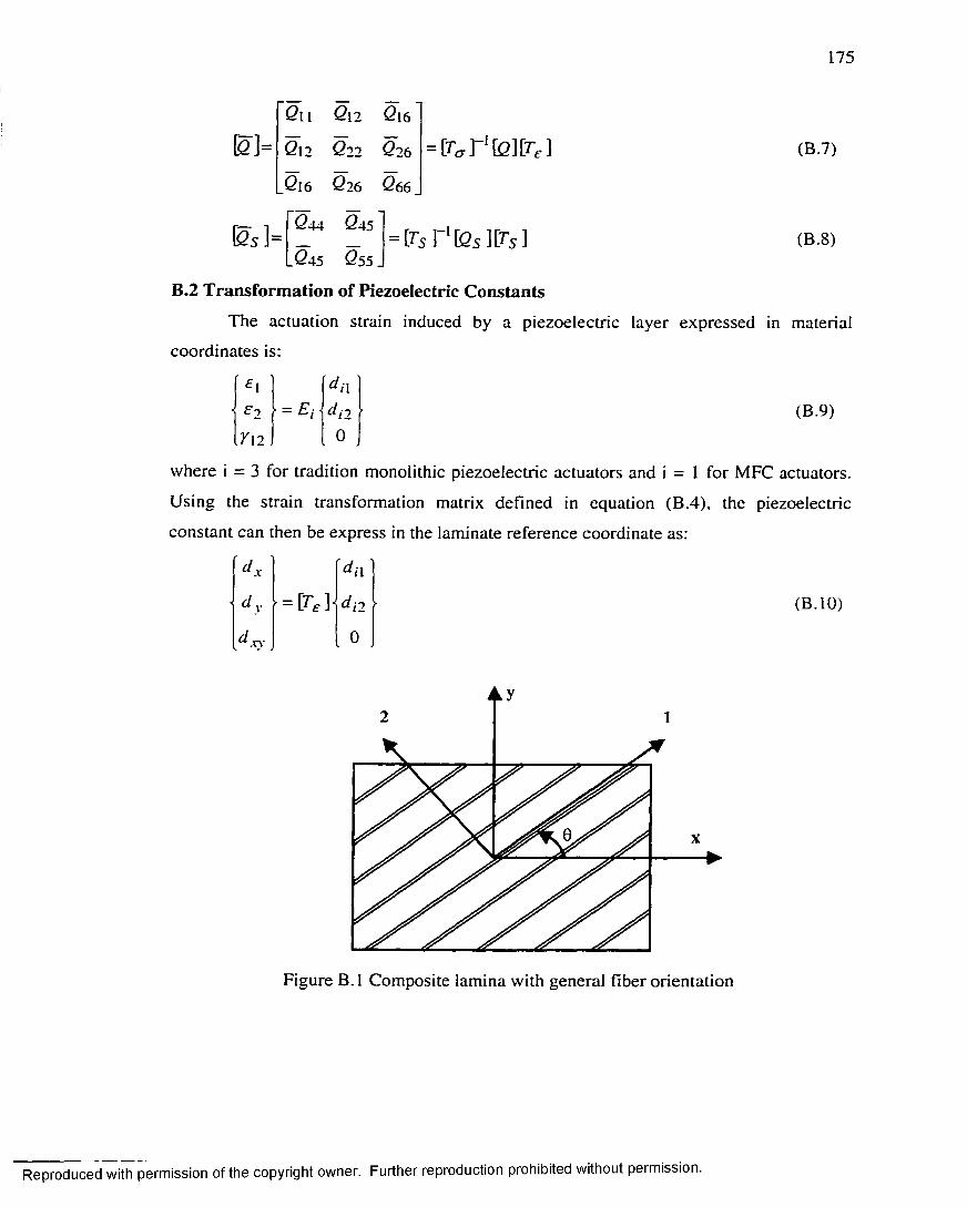
175
= [ T a T l \ Q ] [ T £ ] (B.7)
011 012 016
012 022 026
.016 026 066.
044 045
.045 055.
B.2 Transformation of Piezoelectric Constants
The actuation strain induced by a piezoelectric layer expressed in material
B s h = [TS r l \ Q s ] i T S ] (B.8)
coordinates is:
£1 d i{■ = E r d i l
712 0(B.9)
where i = 3 for tradition monolithic piezoelectric actuators and i = 1 for MFC actuators.
Using the strain transformation matrix defined in equation (B.4), the piezoelectric
constant can then be express in the laminate reference coordinate as:
(B. 10)
d x d a
d y II d \ 2
d x y 0
Figure B. 1 Composite lamina with general fiber orientation
Reproduced with permission of the copyright owner. Further reproduction prohibited without permission.

176
APPENDIX C
SOLUTION PROCEDURE FOR OPTIMAL OUTPUT FEEDBACK
Given the system state space matrices (A, B, C, D), performance index weighting
matrices (Q , R ), and initial conditions distribution (AT0), then the optimal output feedback
gain can be determined using the following iterative solution procedure:
1. Determine an initial stabilizing gain matrix, Ka, such that A-BKaC is stable.
2 . k-th iteration:
- Set A c = A-B{Ky)kC
- Solve for P k and S* matrices using (K y ) k and the following equations:
a J P + PAC + C T K y R K y C + Q = 0
A c S + s a J + X q = 0
- Set Jk = 0.5tr(PkX0)
If | J k - J k - i I < Tolerance, go to step 3, otherwise:
Determine the gain update direction:
AK y = R ~ 1B T P S C T (C S C T r 1 ~ ( K y )k
Update the gain using (K y )k + i = (K y ) k + a A K y
where a is a chosen constant
Repeat step 2
3. Terminate and set Ky= (Ky)k+i
Reproduced with permission of the copyright owner. Further reproduction prohibited without permission.

177
CURRICULUM VITA
for
KHALED ABDEL-MOTAGALY
DEGREES:
• Doctor of Philosophy (Aerospace Engineering), Old Dominion University,
Norfolk, VA, Dec. 2001
• Master o f Science (Aerospace Engineering), Cairo University, Cairo, Egypt, July
1995
• Bachelor o f Science (Aerospace Engineering), Cairo University, Cairo, Egypt, July
1991
PROFESSIONAL CHRONOLOGY:
• Titan Systems Corp.- LinCom division, Houston, TX
Senior Systems Engineer, July 1999 - Present
• Eagle Aeronautics, Newport News, VA
Research Scientist, Jan. 1999 - June 1999
• Aerospace Engineering Dept., Old Dominion University, Norfolk, VA
Research and Teaching Assistant, Jan 1996 - Dec. 1998
• Aerospace Engineering Dept., University o f Cincinnati, Cincinnati, OH
Teaching Assistant, Sept. 1995 - Dec. 1995
• Aerospace Engineering Dept., Cairo University, Cairo, Egypt
Research and Teaching Assistant, Aug. 1991 - Aug. 1995
HONORS AND AWARDS:
• Member o f the national honor society Phi Kappa Phi
• Graduate Scholarship, Old Dominion University, Norfolk, VA, Jan. 1996 - Dec.
1998
• Graduate Scholarship, University of Cincinnati, Cincinnati, OH, Sept. 1995 - Dec.
1995
• Graduate Scholarship, Cairo University, Egypt, Dec. 1992 - Aug. 1995
• Egyptian Engineering Syndicate excellence award for the top aerospace
engineering student, 1991
Reproduced with permission of the copyright owner. Further reproduction prohibited without permission.

178
• Honor degree, Cairo University, Egypt, 1991
• Student of the Year, Aerospace Engineering Department, Cairo University, Egypt,
1990-1991
SCHOLARLY ACTIVITIES COMPLETED:
R e f e r e e d J o u r n a l A r t i c l e s :
• Abdel-Motagaly, K., Duan, B., and Mei, C„ "Nonlinear response of composite
panels under combined acoustic excitation and aerodynamic pressure,” A I A A
J o u r n a l , Vol.38, No.9, Sept. 2000, pp. 1534-1542.
• Abdel-Motagaly, K„ Chen, R., and Mei, C., "Nonlinear flutter o f composite panels
under yawed supersonic flow using finite elements," A I A A J o u r n a l , Vol. 37, No. 9,
Sept. 1999, pp. 1025-1032.
• Mei, C., Abdel-Motagaly, K., and Chen, R., "Review of nonlinear panel flutter at
supersonic and hypersonic speeds,” A p p l i e d M e c h a n i c s R e v i e w , Vol. 52, No 10,
Oct. 1999, pp. 305-332.
• Hassan, S. D., El-Bayoumi, G. M., and Abdel-Motagaly, K., "Two new learning
algorithms for rules generation in self-organizing fuzzy logic controllers,” J o u r n a l
o f E n g i n e e r i n g a n d A p p l i e d S c i e n c e , Faculty of Engineering, Cairo University,
Vol. 43, No. 4, Aug. 1996, pp. 765-780.
• Hassan, S. D„ El-Bayoumi, G. M., and Abdel-Motagaly, K., "Longitudinal
autopilot design for a large scale flexible missile using LQR,” E n g i n e e r i n g
R e s e a r c h J o u r n a l , University of Helwan, Cairo, Egypt, Vol. 5, No. 6 , June 1995,
pp. 91-104.
S e l e c t e d R e f e r e e d P r o c e e d i n g s :
• Abdel-Motagaly, K„ Rombout, O., Gonzalez, R., Berrier, K., Hasan, D., Strack,
D„ and Rishikof, B., "Studies on the Attitude Control System Design for the
Crew Return Vehicle (X38),” A d v a n c e s i n t h e A s t r o n o m i c a l S c i e n c e s , G u i d a n c e
a n d C o n t r o l , Volume 104, 2000, pp. 281-297.
• Abdel-Motagaly, K., Duan, B., and Mei, C., “Nonlinear panel response at high
acoustic excitations and supersonic speeds,” P r o c e e d i n g s o f t h e 4 C fh A I A A
S t r u c t u r e , S t r u c t u r e D y n a m i c s , a n d M a t e r i a l s C o n f e r e n c e , St. Louis, MO, April
1999, pp. 1518-1529.
Reproduced with permission of the copyright owner. Further reproduction prohibited without permission.

179
• Abdel-Motagaly, K., Chen, R., and Mei, C., “Effect o f flow angularity on
nonlinear supersonic flutter o f composite panels,” P r o c e e d i n g s o f t h e 4 ( f h A I A A
S t r u c t u r e , S t r u c t u r e D y n a m i c s , a n d M a t e r i a l s C o n f e r e n c e , St. Louis, MO, April
1999, pp. 1963-1972.
• Aledhaibi, A., Abdel-Motagaly, K., and Huang, J., ’’Design of self-organizing
fuzzy control for robot manipulator,” Proceedings of the 4 t h . J o i n t C o n f e r e n c e o n
I n f o r m a t i o n S c i e n c e s ( J C I S ) , Vol. I, Oct. 1998, Research Triangle Park, NC, pp.
73-75.
• Abdel-Motagaly, K. and Alberts, T., “Robust control design for a flexible
manipulator using Hoo/j.1 synthesis,” P r o c e e d i n g o f t h e A I A A G u i d a n c e ,
N a v i g a t i o n , a n d C o n t r o l C o n f e r e n c e , Boston, Massachusetts, Aug. 1998, pp. 365-
372.
• Abdel-Motagaly, K. and C. Mei, “On the control of nonlinear free vibration of a
simply supported beam,” P r o c e e d i n g s o f t h e 3 9 th A I A A S t r u c t u r e , S t r u c t u r e
D y n a m i c s , a n d M a t e r i a l s C o n f e r e n c e , Long Beach, CA, April 1998, pp. 3266-
3278.
• Lee, R. Y., Abdel-Motagaly, K., and Mei, C., “Fuzzy logic control for nonlinear
free vibration o f composite plates with piezoactuators,” P r o c e e d i n g s o f t h e 3 9 th
A I A A S t r u c t u r e , S t r u c t u r e D y n a m i c s , a n d M a t e r i a l s C o n f e r e n c e , Long Beach,
CA, April 1998, pp. 867-875.
• Hassan, S. D„ El-Bayoumi, G. M., and Abdel-Motagaly, K., “Application of
fuzzy logic control to the longitudinal autopilot o f a large scale flexible missile,”
3 r d I n t e r n a t i o n a l C o n f e r e n c e o n E n g i n e e r i n g M a t h e m a t i c s a n d P h y s i c s , Cairo,
Egypt, Dec. 1997, pp. 296-308.
• Hassan, S. D„ El-Bayoumi, G. M., and Abdel-Motagaly, K., “Attitude control of
large scale flexible missile using self-organizing fuzzy logic control,” 6 th
I n t e r n a t i o n a l C o n f e r e n c e in M e c h a n i c a l D e s i g n a n d P r o d u c t i o n , Cairo, Egypt,
Jan. 1996, pp.741-754.
Reproduced with permission of the copyright owner. Further reproduction prohibited without permission.