BY

JOHN M. KUL.ICKI

CELAL N. KOSTEM

ANALYSIS OF BEAMS

FRITZ -ENGINEERING LABORATORY REPORT No. 378A.5

FURTHER STUDIES ON THE NONLINEAR FINITE ELEMENT

FURTHER STUDIES ON THE NONLINEAR FINITE ELEMENT

ANALYSIS OF BEAMS

by

John M.. Kulicki

Celal No Kostem

This work was conducted as a part of the projectOverloading Behavior of Beam-Slab Highway Bridges,sponsored by the National Science Foundation.

Fritz Engineering Laboratory

Department of Civil Engineering

Lehigh University

Bethlehem, Pennsylvania

April, 1973

Fritz Engineering Laboratory Report No. 378A.5

TABLE OF CONTENTS

ABSTRACT

1. INTRODUCTION

2. THEORETICAL CONSIDERATION

2.1 The Finite Element Method

2.2 Stress-Strain Curves

1

3

3

6

Concrete in Compression

Concrete in Tension

7

8

2.3 Iteration Scheme

3. PARAMETRIC STUDY

3.1 Introduction and Scope

3 .. 2 The Effect of Iteration Tolerance

3 .. 3 The Effect of a Uniform Load

3,,4 The Effect of Reinforcement Yield Point - fs

3 .. 5 The Effect of Draped Strand

3.6 The Effect of Varying CompressiveStress-Strain Par~meters

3.6 .. 1 The Effect of HmH

3 .. 6.2 The Effect of Compressive Strength - £1C

3.6.3 The Effect of TTN TT

3 0 6,,4 The Effect of Youngfs Modulus -- E3.6.5 The Effect of Varying the Analytic

Compressive Stress-Strain Curve

3.7 The Effect of Tensile Stress Tolerance - FTOL

3.8 The Effect of Tensile Strength - Ft3~9 The Effect of Elemental Discretization

10

12

12

15

18

19

20

21

21

24

25

26

26

28

29

29

3010

3.11

3.12

3.13

The Effect of Concrete Layer Discretization

The Effect of Reinforcement Discretization

The Effect of Tensile andCompressive Unloading

The Effect of the Rate ofCompressive Unloading

Comparison with a Laboratory Test ofa Steel Wide Flange Beam

36

38

40

43

44

4. CONCLUSIONS FROM THE PARAMETRIC STUDY 49

401

4.2

4.3

4.4

4.5

4.6

4.7

4.8

4.9

4.10

Iteration Tolerance

Yield Point of Prestressing Strand,Draped Strand and Uniform Loads

Stress-Strain Curve Parameters

Effect of Estimating Material Properties

Tensile Tolerance

Elemental Discretization

Number of Layers

Cracking and Crushing InducedStress Unloading

Steel Wide Flange Beam

General Comments

49

49

49

50

50

50

51

51

52

52

5. FIGURES

6. REFERENCES

7 . ACKNOWLEDGMENTS

S3

103

105

1. INTRODUCTION

This report contains a parametric study conducted using

program BEAM. This program performs an inelastic load deflection

analysis on nonhomogeneous beams or beam-columns using an incre­

mental, iterative, tangent stiffness Finite Element analysis. A

layered beam element is used. The method is based on the assump­

tion that plane sections is an adequate representation of the

cross-sectional strain field and that the cross section is symmet­

ric about the plane of loading. Previous work on other theoreti­

cal considerations pertaining to the method of analysis used in

the computer program and comparisons of analytic and experimental

load deflection curves for two reinforced and eleven prestressed

concrete beams were reported in Ref. 8. Reference 9 is a userTs

manual which describes the application of the program. An exten­

sion of the method to the inelastic analysis of beam-columns has

been reported in Refs 10. A working knowledge of Ref. 8 would

serve as a desirable background to the material contained in this

report.

Chapter 2 contains a review of relevant theory and a

brief description of the iteration scheme used in the computer

program. Chapter 3 contains the results of varying selected para­

meters used (a) to describe the material stress-strain curves,

(b) to model the beam or beam-column to be analyzed, or (c) to de­

scribe internal processing within the program!o Results of several

-1-

other investigation and a comparison with a laborat"ory test of a

steel wide flange beam are also presented. Chapter 4 contains

conclusions drawn from this parametric study.

The computer work used to generate this study was per­

formed on the CDC 6400 installation at the Lehigh University Com­

puting Center. The SCOPE 303 operating system (Ref. 3) and the

RUN (Ref. 1) and FTN (Ref. 2) compilers were used.

-2-

2. THEORETICAL CONSIDERATION

This chapter is essentially the same as Chapter 3 of

Ref. 10. Both of these chapters are a condensation of a detailed

theoretical derivation presented in Ref. 8.

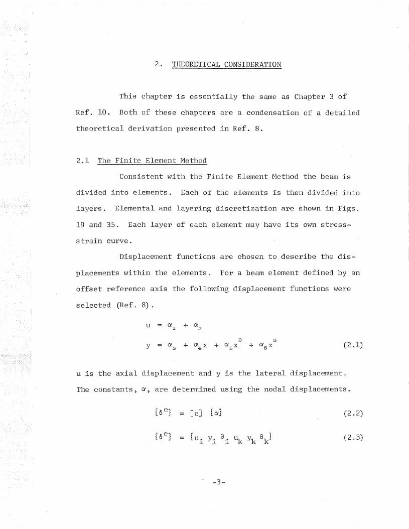
2.1 The Finite Element Method

Consistent with the Finite Element Method the beam is

divided into elements. Each of the elements is then divided into

layers. Elemental and layering discretization are shown in Figs.

19 and 35. Each layer of each element may have its own stress-

strain curve.

Displacement functions are chosen to describe the dis­

placements within the elements. For a beam element defined by an

offset reference axis the following displacement functions were

u is the axial displacement and y is the lateral displacement.

The constants, a, are determined using the nodal displacements.

selected (Ref. 8).

2 3Y = Q'3 + C'4 X + C\l5 X + U'e X (2.1)

(2.2)

(2.3)

-3-

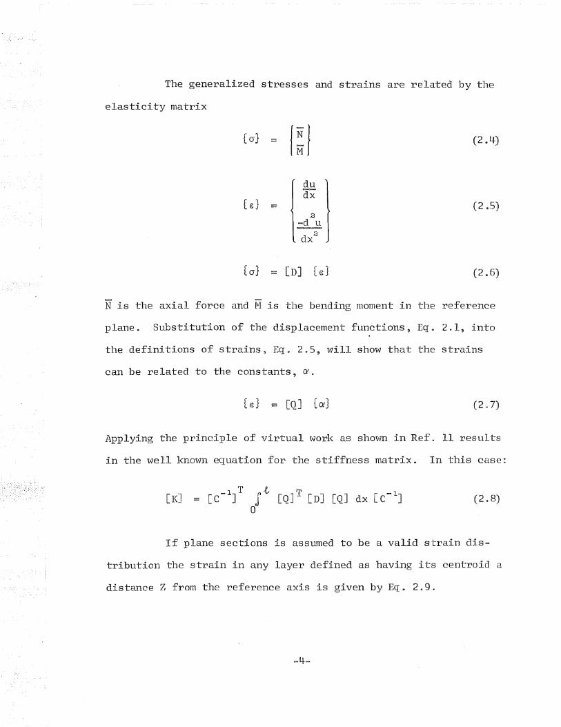
The generalized stresses and strains are related by the

elasticity matrix

(2.4)

(2 .5)

(2.6)

N is the axial force and M is the bending moment in the reference

plane. Substitution of the displacement functions, Eg. 2.1, into

the definitions of strains, Eqo 2.5, will show that the strains

can be related to the constants, a.

[e} = [Q] {Of} (2.7)

Applying the principle of virtual work as shown in Ref. 11 results

in the well known equation for the stiffness matrix. In this case:

(2.8)

If plane sections is assumed to be a valid strain dis-

tribution the strain in any layer defined as having its centroid a

distance Z from the reference axis is given by Ego 2.9.

-4-

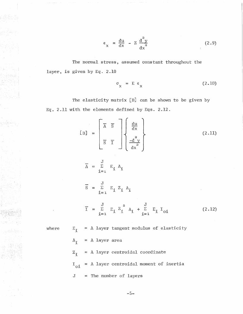
€X = du

dx

2

Z 3-Y2

dx(2.9)

The normal stress, assumed constant throughout the

layer, is given by Eq. 2.10

(J = E ex x

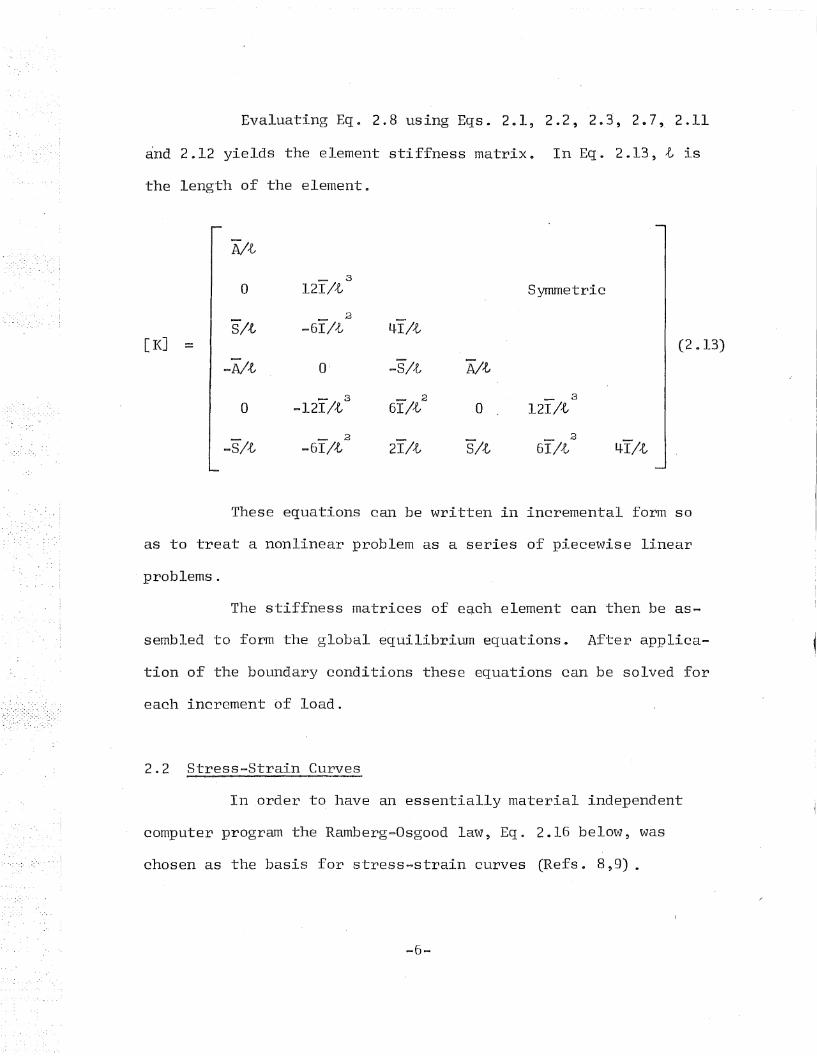
The elasticity matrix [D] can be shown to be given by

Eg. 2.11 with the elements defined by Egs. 2.12.

A S

[D] :::

S I

dudx

2

.::S!-Y2

dx

(2 .11)

JA ::: ~

i=lE. A.

1 1

JS = ~

i::: 1

E. z. A.111

I :::

J~

i:::l

2

E. Z.1 1

JA. + 2:

1 i:::lE. I .

1 01(2 .12)

where E. ::: A layer tangent modulus of elastici ty1

A. ::: A layer area1

Z. = A layer centroidal coordinate1

I . ::: A layer centroidal moment of inertia01

J ::: The number of layers

-5-

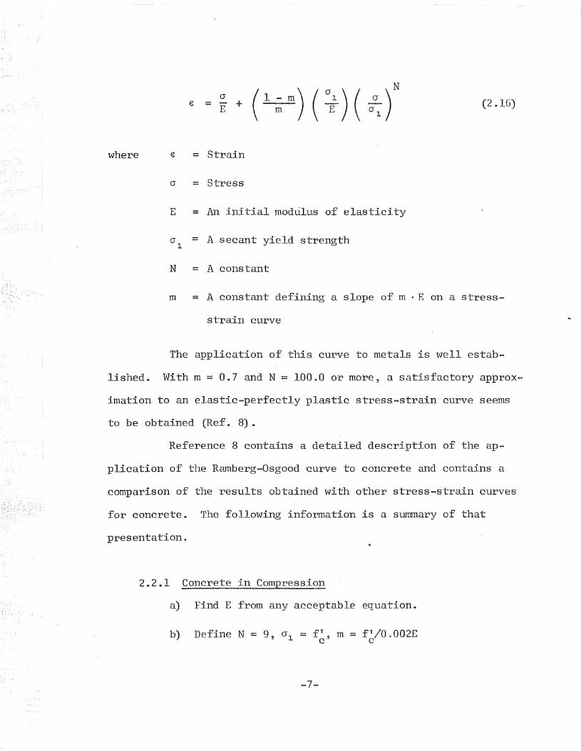
Evaluating Eg. 2.8 using Egs. 2.1, 2.2, 2.3, 2.7, 2.11

and 2.12 yields the element stiffness matrix. In Eg. 2.13, t is

the length of the element.

A!0

12I/{,3

0 Symmetric

sit -6I/-t2

41/t[K] = (2 .13)

-Aft 0 -sit A!t- 3

6f/~2

12I'/t3

0 -121/t 0

-sit -61/t2

21/t sit 6I/t2

41/t

These equations can be written in incremental form so

as to treat a nonlinear problem as a series of piecewise linear

problems.

The stiffness matrices of eqch element can then be as-

sembled to form the global equilibrium equations. After applica-

tioll of the boundary conditions these equations can be solved for

each increment of load.

2.2 Stress-Strain Curves

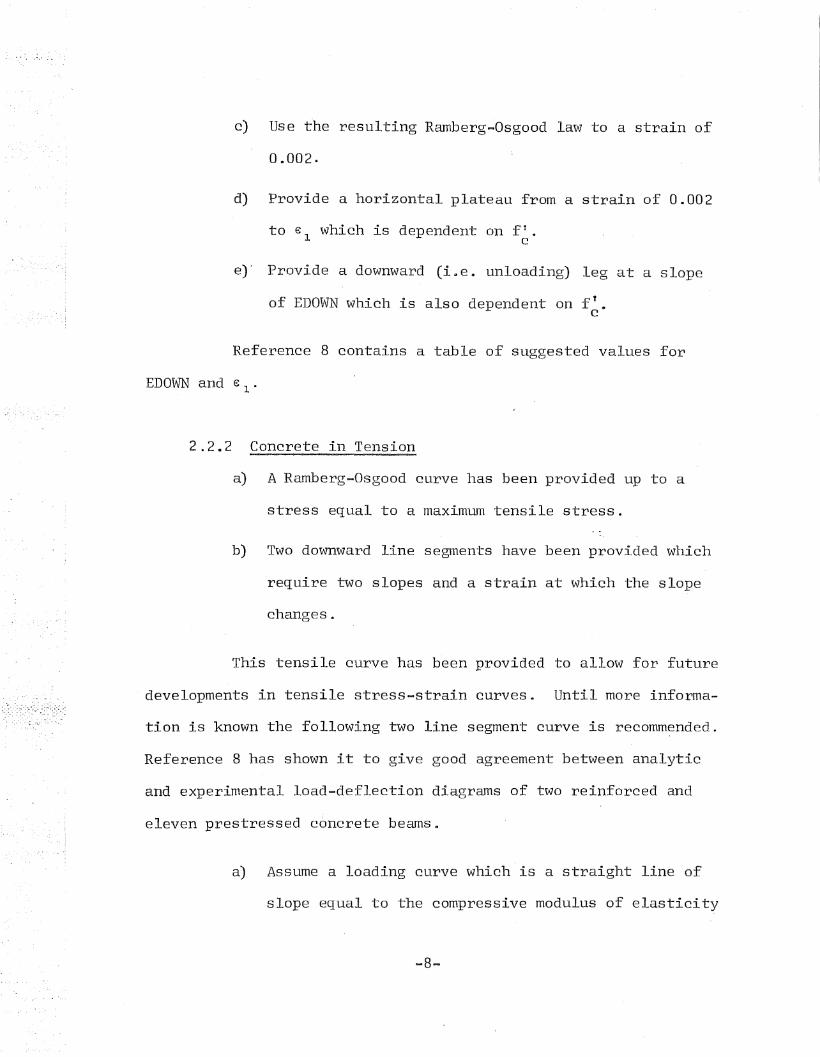
In order to have an essentially material independent

computer program the Ramberg-Osgood law, Eg. 2.16 below, was

chosen as the basis for stress-strain curves (Refs. 8,9).

-6-

(2 .16)

where e = Strain

(J = Stress

E = An initial modulus of elasticity

(J = A secant yield strength1

N = A constant

m = A constant defining a slope of m · E on a stress-

strain curve

The application of this curve to metals is well estab-

lished. With m = 0.7 and N = 100eO or more, a satisfactory approx-

imation to an elastic-perfectly plastic stress-strain curve seems

to be obtained (Ref. 8).

Reference 8 contains a detailed description of the ap-

plication of the Ramberg-Osgood curve to concrete and contains a

comparison of the results obtained with other stress-strain curves

for concrete. The following information is a summary of that

presentation.

2.2.1

a)

b)

Concrete in Compression

Find E from any acceptable equation.

Define N = 9, G 1 = f1, m = f'/0.002£c c

-7-

c) Use the resulting Ramberg-Osgood law to a strain of

0.002.

d) Provide a horizontal plateau from a strain of 0.002

to 8 1 which is dependent on f~.

e)' Provide a downward (ioe. unloading) leg at a slope

of EDOWN which is also dependent on f1.C

Reference 8 contains a table of suggested values for

2.2.2 Concrete in Tension

a) A Ramberg-Osgood curve has been provided up to a

stress equal to a maximum tensile stress.

b) Two downward line segments have been provided which

require two slopes and a strain at which the slope

changes.

This tensile curve has been provided to allow for future

developments in tensile stress-strain curves. Until more informa-

tion is known the following two line segment curve is recomm~nded.

Reference 8 has shown it to give good agreement between analytic

and experimental load.-deflection diagrams of two reinforced and

eleven prestressed concrete beams.

a) Assume a loading curve which is a straight line of

slope equal to the compressive modulus of elasticity

-8-

and terminating at the maximwn tensi-le stress. Set­

ting m = 1.0, 01 = Ft in the Ramberg-Osgood curve

with IT S- Ft will provide this straight line.

b) Assume an unloading curve which is linear downward

at a slope, EDOWNT, of 800.0 ksi.

Strain hardening can also be handled by supplying a nega­

tive slope on the downward legs used in the tensile and compressive

stress-strain curves. Reference 9 contains a detailed description

of the options allowed by the original computer program.

The downward legs of the stress-strain curves are used

to convert strain increments into tfficticious stresses" which are

in turn used to unload layers which have been found to exceed

cracking or crushing criteria. The TTficticious stre~sesTT are also

used to compute nodal forces which hold the rest of the beam in

equilibrium. -This process produces a globally adequate but not

locally exact redistribution of stresses.

Each layer may have its own stress-strain curve. In

this way non-homogeneous beams or beam-columns can be analyzed.

The assumption of plane sectio~s implies, of course, that no rela­

tive slip between materials of a given beam-column may occur.

When dealing with concrete members this means that perfect bond

has been assumed.

-9-

2.3 Iteration Scheme

The iteration procedure for a given load increment is

started by solving the global equilibrium equations for the incre­

ments of displacement (Refs. 8,9). Strain increments are computed

from the displacement increments. Using the latest level of

stress available new tangent moduli are computed for each layer,

the global stiffness matrix is regenerated and the equilibrium

equations are solved again. If the new increments of displacement

are within a relative tolerance of the previous set, convergence

is said to have occurred. If convergence has not occurred ·the

process is repeated. If convergence is not attained in several

trials the load increment is reduced and the process is repeated.

If no convergence is attained after a number of reductions in load

the process is stopped. If convergence is attained in relatively

few trials the load increment to be applied for the next load step

is increased so as to reduce the total number of load steps used.

Once convergence has been attained for the load step,

consideration is given to cracking and crushing if appropriate.

The first phase in this step is a pre-scanning process in which

all the layers are checked to see if they have exceeded the allow­

able tensile or compressive stress tolerances by an excessive

amount. If this occurs the basic load step is reduced and the pro­

blem of finding a converged displacement increment for the basic

load step is repeated.

-10-

Once it has been determined that no stress criteria are

exceeded by more than their tolerances any alteration in stiffness

required by the cracking or crushing of a layer is made. The

TTficticious forces TT described in Ref. 8 are computed. The global

equilibrium problem corresponding to that set of TTficticious

forces TT is solved until convergence is attained. The layers are

then rechecked to see if subsequent cracking or crushing has 'oc­

curred. If so the cracking-crushing analysis is repeated. It is

the process of cracking generating more cracking and/or crushing

generating more crushing which simulates the in-plane instability

condition in concrete beams.

Alterations in the stiffness matrix arising from plastic

flow like phenomena are aut?matically accounted for by employing

the appropriate Ramberg-Osgood curve o

A detailed description of the computer program which

performs this analysis as well as the input required and the out­

put generated can be found in Ref. 9.

-11-

3. PARAMETRIC STUDY

3.1 Introduction and Scope

This chapter describes a parametric study conducted with

and on program BEAM (Refs. 8,9). The object of this study is

twofold:

1. To investigate the sensitivity of the analysis technique

to such variables as elemental discretization.

2. To investigate the behavior of beams when one or more

characteristic parameters are altered.

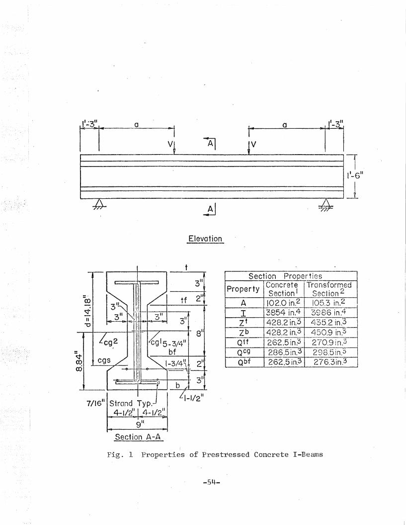
All investigations were carried Qut_ using the prestressed

concrete I-beam E-5 discussed in Ref. 8 and shown in Fig. 1, except

as noted. In most cases the two concentrated loads shown in Fig.

1 were applied with the distance natf equal to four feet. In some

cases a uniform load was applied. Most of the values of applied

load in the figures to be presented are given as a TTload ratioTT.

A load ratio is defined as the value of one of the concentrated

loads, V, shown in Fig. 1 divided by 20., or the value of a uni­

form load divided by the starting value of its intensity. Two

different length uniformly loaded beams will be considered. For

the beam which is 12 ft. 6 in. long the starting value of uniform

load intensity was 4.5 kips per foot. For the beam which· was 17

ft. 6 in. long the starting value was 2.4 kips per foot. All de­

flections and positions given in the figures are in inches.

-12-

The parameters investigated in this report are listed

below:

1. The effect of the variation of the iteration tolerance

using values of 1%, 5%, 10%, and 20%·.

2. The effect of a uniform load, as opposed to third point

loading (Ref. 8).

3. The effect of varying the yield strength of the strand

from 225. to 265. ksi.

4. The effect of draped strand, as opposed to straight

strand.

5. The effect of the variation of the Ramberg-Osgood para­

meter TTmTT for the values of 0.52, 0.72, and 0.92.

6. The effect of the variation of the Ramberg-Osgood para­

meter uN TT using the values of 7.0, 9.0, and 11.0.

7. The effect of varying the compressive strength of the

concrete ±600. psi from the base value of 6,610. psi.

8. The effect of varying Youngfs modulus ±600. ksi from the

base value of 4600. ksi.

9. The effect of varying the compressive strength ±600. psi

and using the procedure discussed in Section 2.2.1 to

compute the other stress-strain curve parameters.

10. The effect of the variation of the tolerance on the ten­

sile strength for the values of 1%, 10%, and 20%.

-13-

11. The effect of varying the tensile strength of the con­

crete ±lOO. psi from the base value of 530. psi.

12. The effect of using 2, 4, and 8 elements of equal length

with a small element at the centerline.

13. The effect of using 2, 4, and 8 elements of equal length

with a small element at a support.

14. The effect of using 3 steel layers with 6, 9, and 12

concrete layers.

15. The effect of using 12 concrete layers with 1, 2, and 3

steel layers.

16., The effect of no compressive unloading, no tensile un­

loading, no compressive and no tensile unloading and,

finally, including both types of unloading.

17. The effect of varying the rate of compressive unloading

from 1000. ksi to 4000. ksi.

Each of these studies will now be discussed in detail.

The laboratory test beams used as comparative standards

in this study all exhibited under-reinforced behavior. Needless

to say some of the conclusions drawn here would be different for

over-reinforced beams. In general, those conclusions dealing with

small changes in external load and involving the yielding of the

strand should be regarded as being especially applicable to the

under-reinforced case.

-14-

It will also be noticed that many of the load deflection

curves presented in this report have a short, almost horizontal

plateau after the original essentially linear response. As ex­

plain~d in Ref. 8, this is largely a result of the discretization

used and an approximation made for the dead load bending stress.

Comparisons with laboratory tests of I-beams contained in Ref. 8

have shown that this plateau does not alter the generally excel­

lent agreement between analytic and experimental load deflection

curves.

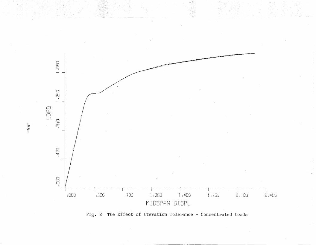
3.2 The Effect of Iteration Tolerance

Figure 2 shows the effect of varying the convergence

tolerance on the load deflection diagram. The four curves shown

correspond to 1%, 5%, 10%, and 20% relative error tolerance on the

displacement field. It can be seen that this wide range of error

tolerance has a surprisingly small effect on the load-deflection

curve for the centerline of the beam. This can be explained as

follows:

1. The incremental displacement vector is initially null for

each increment of load. This means that the first itera­

tion of each increment is never accepted as meeting the

error tolerance. If the final vector from the preceding

trial were used as the comparative standard it is appar­

ent that many trials could be within say a 10% tolerance

-15-

of this standard on the first iteration of the next load

step. The null initial vector requires more computational

effort but the results seem to justify it. Experience

has shown that perhaps one-third of the load steps are

solved with only two iterations making it even more appar­

ent that the error tolerance insensitivity is related to

the null initial incremental displacemen~ vector.

2. The error tolerance is the maximum allowed for any dis­

placement. This means that most, and possibly all, of

the other displacements have less than the maximum error.

3. The error tolerance is a relative, absolute value so that

the error could b~ positive or negative. This would re­

duce the accumulation of error in some indefinable manner.

It would not, however, increase the accumulation of error.

4. The same displacement component would probably not consis­

tently be the one with the maximum error. This would

tend to distribute the error and aid in making the accumu­

lated error significantly smaller than the maximum allow­

able error.

s. Figure 2 shows the effect on midspan vertical defl~ction

which is the largest displacement component for this beam.

It seems plausable that the smaller values would be more

susceptible to error than the larger ones. It might

-16-

therefore be possible to plot some other displacement and

see a greater effect of the error tolerance.

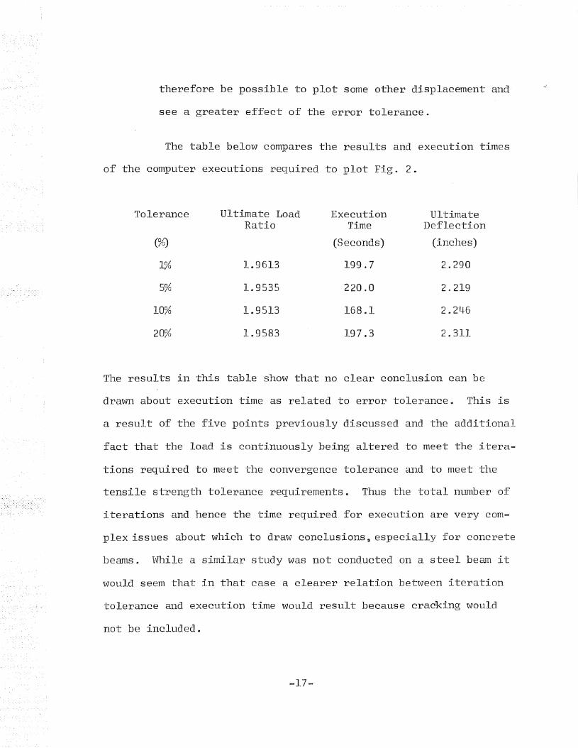
The table below compares the results and execution times

of the computer executions required to plot Fig. 2.

Tolerance Ultimate Load Execution UltimateRatio Time Deflection

(%) (Seconds) (inches)

1% 1.9613 199.7 2.290

5% 1.9535 220.0 2.219

10% 1.9513 168.1 2.246

20% 1.9583 197.3 2.311

The results in this table show that no clear conclusion can be

drawn about execution time as related to error tolerance. This is

a result of the five points previously discussed and the additional

fact that the load is continuously being altered to meet the itera-

tions required to meet the convergence tolerance and to meet the

tensile strength tolerance requirements. Thus the total number of

iterations and hence the time required. for execution are very com-

plex issues about which to draw conclusions, especially for concrete

beams. While a similar study was not conducted on a steel beam it

would seem that in that case a clearer relation between iteration

tolerance and execution time would result because cracking would

not be included.

-17-

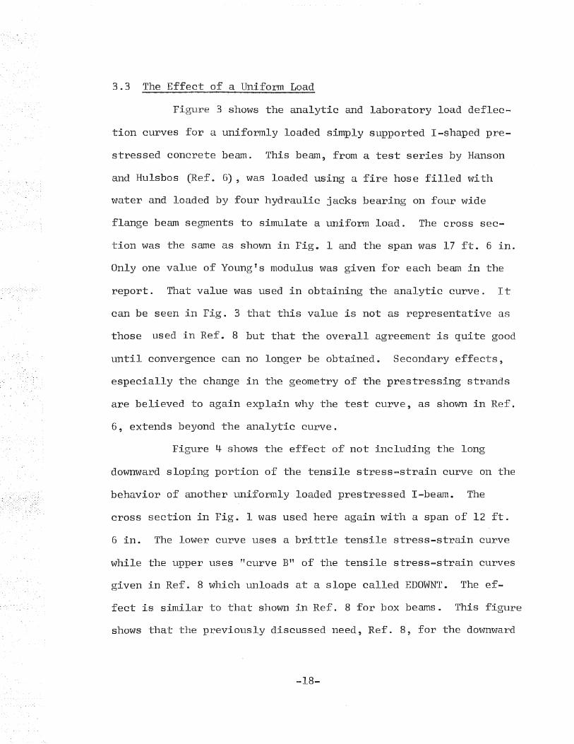
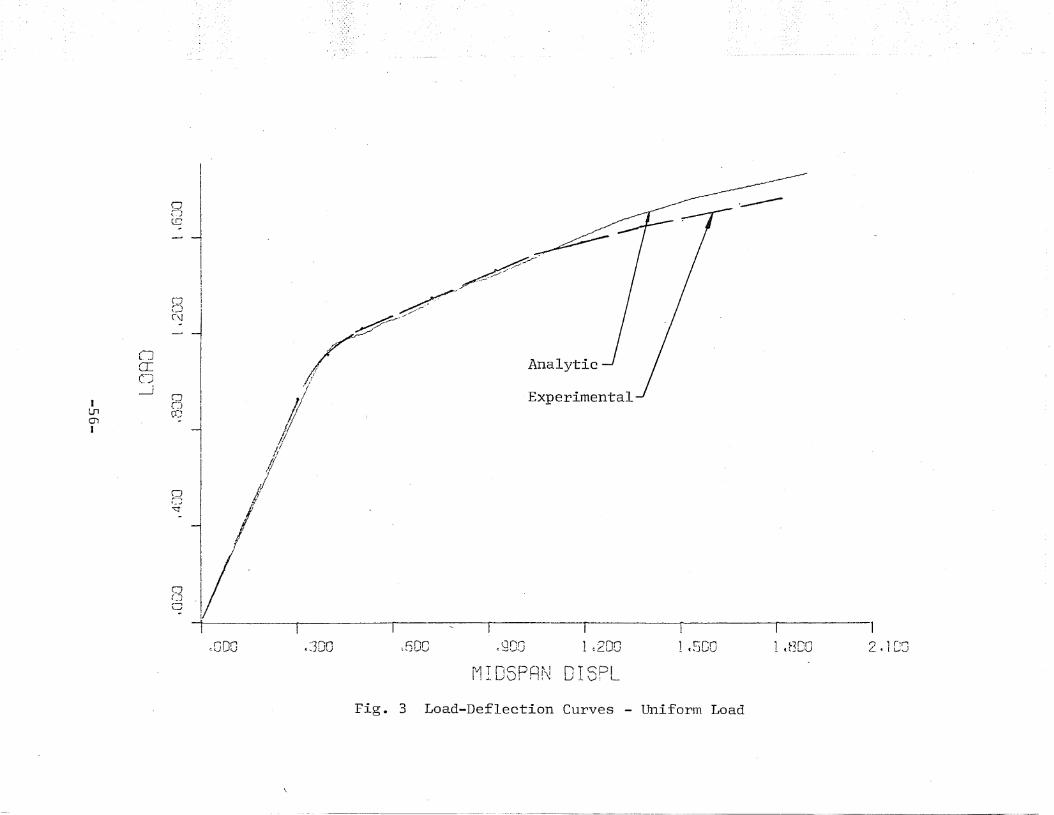
3.3 The Effect of a Uniform Load

Figure 3 shows the analytic and laboratory load deflec-

tioD curves for a uniformly loaded simply supported I-shaped pre-

stressed concrete beam. This beam, from a test series by Hanson

and Hulsbos (Ref. 6), was loaded using a fire hose filled with

water and loaded by four hydraulic jacks bearing on four wide

flange beam segments to simulate a uniform load. The cross sec-

tion was the same as shown in Fig. 1 and the span was 17 ft. 6 in.

Only one value of YoungTs modulus was given for each beam in the

report. That value was used in obtaining the analytic curve. It

can be seen in Fig. 3 that this value is not as representative as

those used in Ref. 8 but that the overall agreement is quite good

until convergence can no longer be obtained. Secondary effects,

especially the change in the geometry of the prestressing strands

are believed to again explain why the test curve~ as shown in Ref.

6, extends beyond the analytic curve.

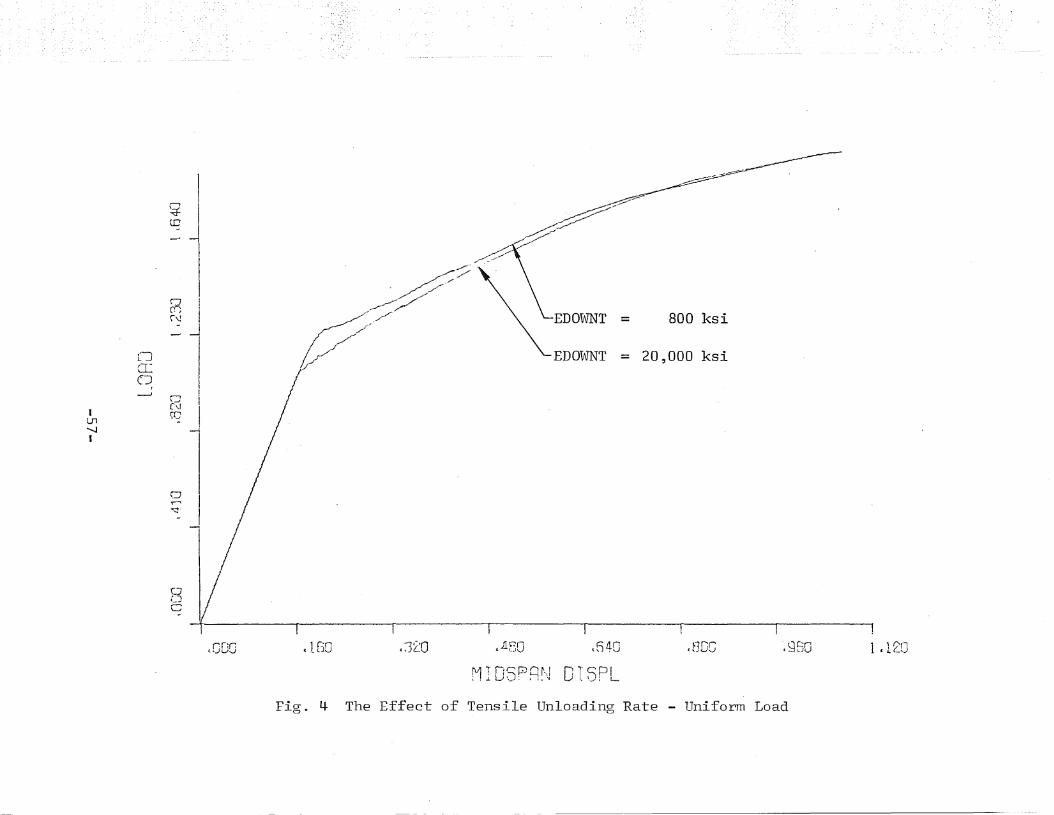
Figure 4 shows the effect of not including the long

downward sloping portion of the tensile stress-strain curve on the

behavior of another uniformly loaded prestressed I-beam. The

cross section in Fig. 1 was used here again with a span of 12 ft.

6 in. The lower curve uses a brittle tensile stress-strain curve

while the upper uses Hcurve Eft of the tensile stress-strain curves

given in Ref. S which unloads at a slope called EDOWNT. The ef-

fect is similar to that shown in Ref. S for box beams. This figure

shows that the previously discussed need, Ref. 8, for the downward

-18-

leg of concrete tensile stress-strain curves is not an outgrowth

of the pure bending loading used in the comparisons with the labo­

ratory tests included in Ref. 8.

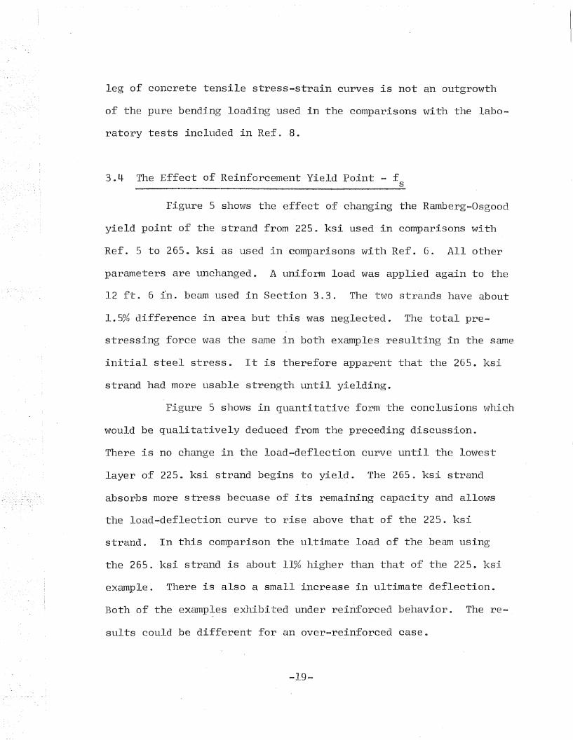
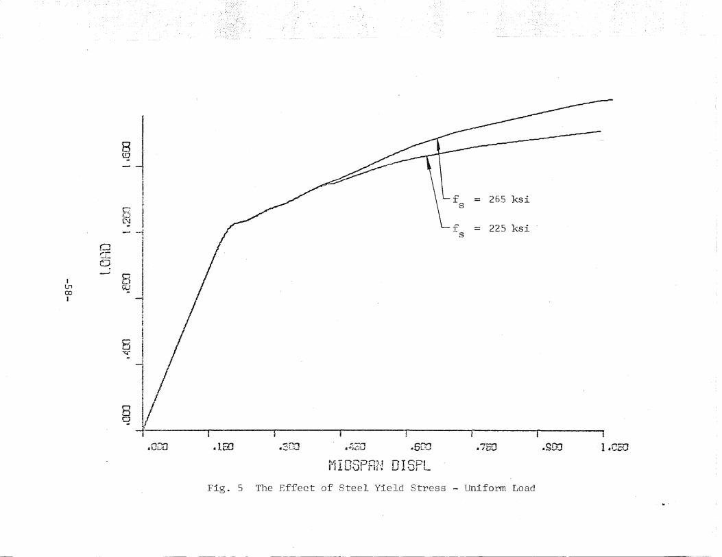
3.4 The Effect of Reinforcement Yield Point - f s

Figure 5 shows the effect of changing the Ramberg-Osgood

yield point of the strand from 225. ksi used in comparisons with

Ref. 5 to 265. ksi as used in comparisons with Ref. 6. All other

parameters are unchanged. A uniform load was applied again to the

12 ft. 6 In. beam used in Section 3.3. The two strands have about

1.5% difference in area but this was neglected. The total pre­

stressing force was the same in both examples resulting in the same

initial steel stress. It is therefore apparent that the 265. ksi

strand had more usable strength until yielding.

Figure 5 shows in quantitative form the conclusions which

would be qualitatively deduced from the preceding discussion.

There is no change in the load-deflection curve until the lowest

layer of 225. ksi strand begins to yield. The 265. ksi strand

absorbs more stress becuase of its remaining capacity and allows

the load-deflection curve to rise above that of the 225. ksi

strand. In this comparison the ultimate load of the beam using

the 265. ksi strand is about 11% higher than that of the 225. ksi

example. There is also a small 'increase in ultimate deflection.

Both of the examples exhibited under reinforced behavior. The re­

sults could be different for an over-reinforced case.

-19-

This example contains results similar to those which

would be expected from using untensioned strand to improve the

ultimate moment capacity of a given prestressed concrete beam.

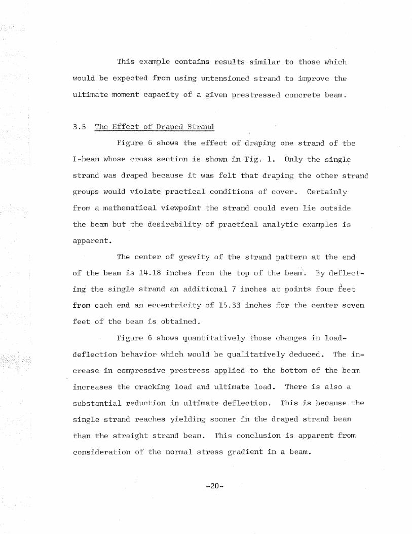
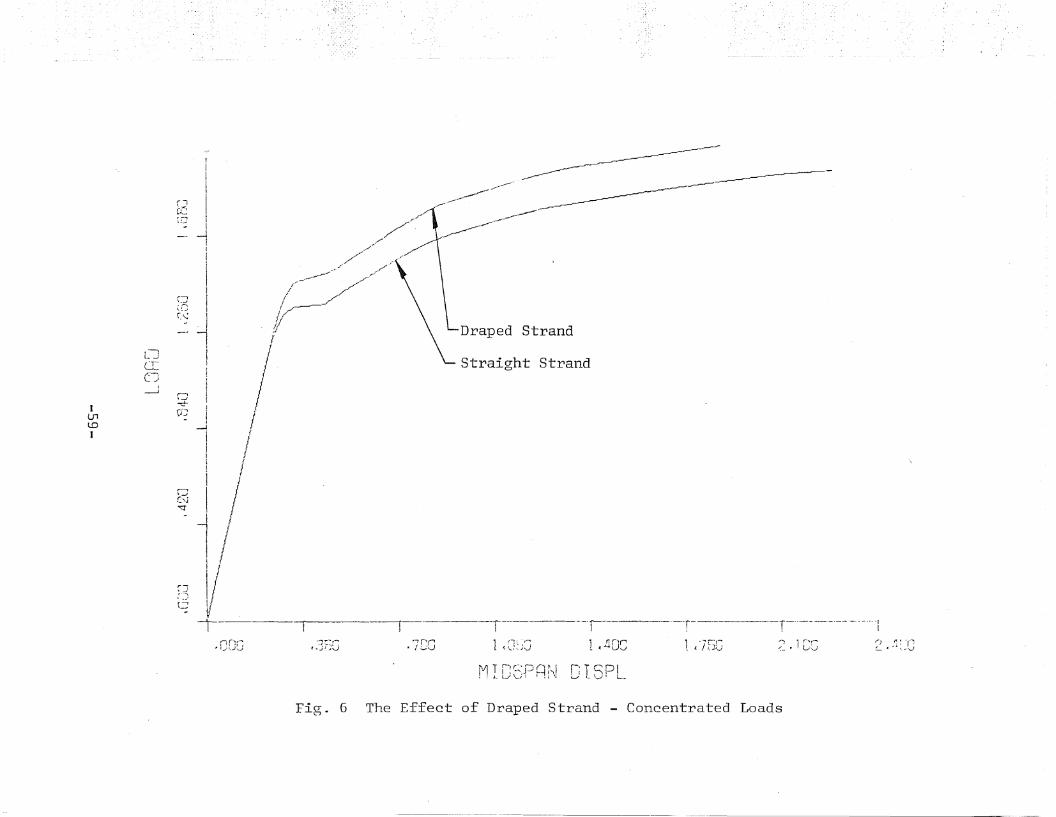
3.5 The Effect of Draped Strand

Figure 6 shows the effect of draping one strand of the

I~beam whose cross section is shown in Fig. 1. Only the singl~

strand was draped because it was felt that draping the other strand

groups would violate practical conditions of cover. Certainly

from a mathematical viewpoint the strand could even lie outside

the beam but the desirability of practical analytic examples is

apparent.

The center of gravity of the strand pattern at the end

of the beam is 14.18 inches from the top of the bean1". By deflect­

ing the single strand an additional 7 inches at points four feet

from each end an eccentricity of 15.33 inches for the center seven

feet of the beam is obtained.

Figure 6 shows quantitatively those changes in load­

deflection behavior which would be qualitatively deduced. The in­

crease in compressive prestress applied to the bottom of the beam

increases the cracking load and ultimate load. There is also a

substantial reduction in ultimate deflection. This is because the

single strand reaches yielding sooner in the draped strand beam

than the straight strand beam. This conclusion is apparent from

consideration of the normal stress gradient in a beam.

-20-

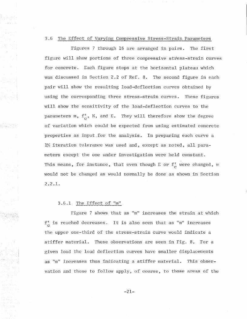
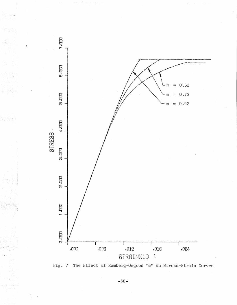
3.6 The Effect of Varying Compressive Stress-Strain Parameters

Figures 7 through 16 are arranged in pairs. The first

figure will show portions of three compressive stress-strain curves

for concrete. Each figure stops at the horizontal plateau which

was discussed in Section 2.2 of Ref. 8. The second figure in each

pair will show the resulting load-deflection curves obtained by

using the corresponding three stress-strain curves. These figures

will show the sensitivity of the load-deflection curves to the

parameters m, fT, N, and E. They will therefore show the degreec

of variation which could be expected from using estimated concrete

properties as input/for the analysis. In preparing each curve a

1% iteration tolerance was used and, except as noted, all para-

meters except the one under investigation were held constant.

This means, for instance, that even though E or f1 were changed~ mc

would not be changed as would normally be done as shown in Section

2.2.1.

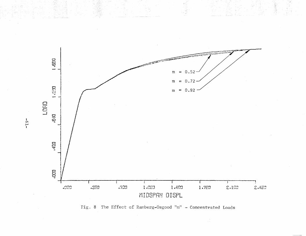
3.6.1 The Effect of TTmTT

Figure 7 shows that as TTmtT increases the strain at which

fT is reached decreases. It is also seen that as TTmTT increasesc

the upper one-third of the stress-strain curve would indicate a

stiffer material. These observations are seen in Fig'. 8. For a

given load the load deflection curves have smaller displacements

as TTmTT increases thus indicating a stiffer material. This obser-

vation and those to follow apply, of course, to those areas of the

-21-

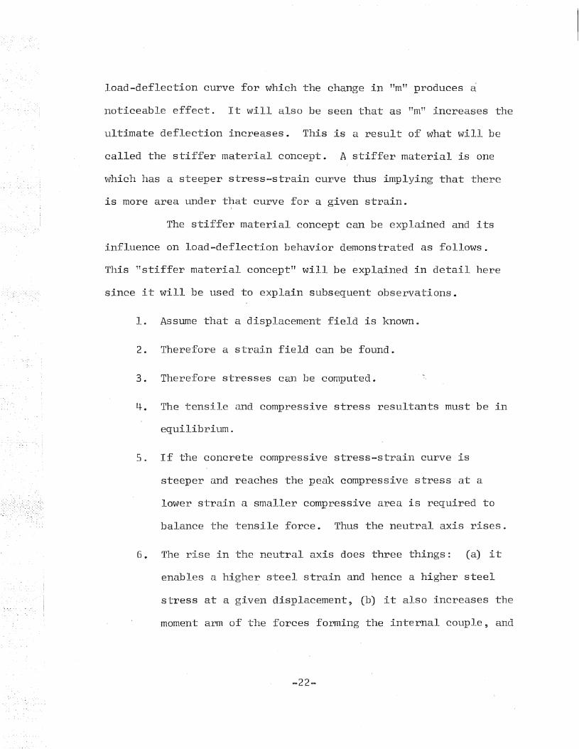
load-deflection curve for which the change in TTmTT produces a

noticeable effect.. It will also be seen that as tTmTT increases the

ultimate deflection increases. This is a result of what will be

called the stiffer material concept. A stiffer material is one

which has a steeper stress-strain curve thus implying that there

is more area under that curve for a given strain.

The stiffer material concept can be explained and its

influence on load-deflection behavior demonstrated as follows.

Tllis TTstiffer material concept TT will be explained in detail here

since it will be used to explain subsequent observations.

1. Assume that a displacement field is known.

2. Therefore a strain field can be found.

3. Therefore stresses can be computed.

4. The tensile and compressive stress resultants must-be in

equilibrium.

5. If the concrete compressive stress-strain curve is

steeper and reaches the peak compressive stress at a

lower strain a smaller compressive area is required to

balance the tensile force. Thus the neutral axis rises.

6. The rise in the neutral axis does three things: (a) it

enables a higher steel strain and hence a higher steel

stress at a given displacement, (b) it also increases the

moment arm of the forces forming the internal couple, and

-22-

(c) while the steel strain is higher the concrete strain

can be lower with a stiffer material and still produce a

given compressive resultant. All of these actions contri­

bute to the support of a larger external load at a given

displacement or, conversely, a lower displacement at a

given load.

7. At the load required for the less stiff stress-strain

curve to reach unloading the stiffer stress-strain curve

would have resulted in a lower displacement and a lower

st~ain. Even when a beam made of the stiffer material

reaches a deflection corresponding to the ultimate deflec­

tion of the less stiff beam the concrete strain is still

lower because of the higher neutral axis. Therefore, it

takes a larger displacement to reach the unloading portion

of the stress-strain curve and hence the ultimate load of

the stiffer material beam. The increase in ultimate de­

flection is 'much larger than the increase in ultimate

load in the example being discussed.

It will also be observed that in the variation of 11 mTT the

stiffer material produces load-deflection curves which approach

their ultimate load at a lower gradient than the less stiff mate­

rial. This is caused by the fact that the stiffer curves resulting

from a higher TTmTT reached their horizontal plateau at a somewhat

lower strain than the less stiff curves and hence cause a reduced

-23-

stiffness when they reach that plateau. It is also noted that

this plateau is longer for higher values of TTmTT.

For m = 0.52 Fig. 7 also shows that while the observa-

tions above hold for this case too they are exaggerated by the

smaller compressive stress at ultimate load. This explains why

the difference in ultimate load is greater in the pair m = 0.52,

m = 0.72 than in the pair m = 0.72, m = 0.92.

The change in ultimate load is quite small in this under-

reinforced example. This is because internal equilibrium must be

maintained as the steel yields. Thus the total ultimate tensile

and compressive stress resultants would be essentially the same for

all values of TTm1T. But as seen in Fig. 7 the moment arm of the

internal couple would tend ~o increase slightly as TTmTf increases..

and as the ultimate load is reached. This results In a slightly

higher ultimate moment as TTmTT increases.

Figure 8 shows that variation of TTmTT from 0.52 to 0.92

has relatively little effect on the shape of the load deflection

curve except, perhaps, at the ultimate load. If the recommenda-

tions in Ref. 8 on defining the compressive stress-strain curve

are followed the value of TTmTT will be found as shown in Section

2.2.1 of this report an'd will not be subject to judgment.

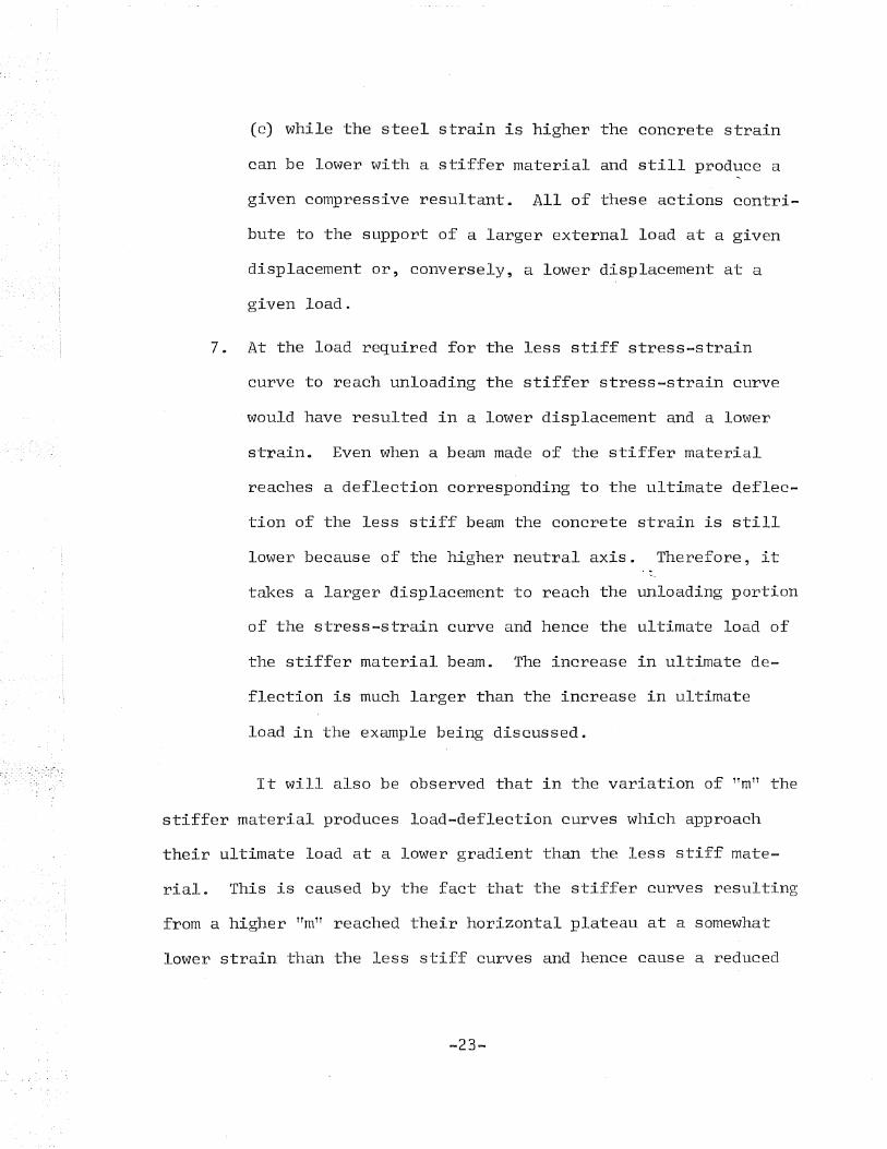
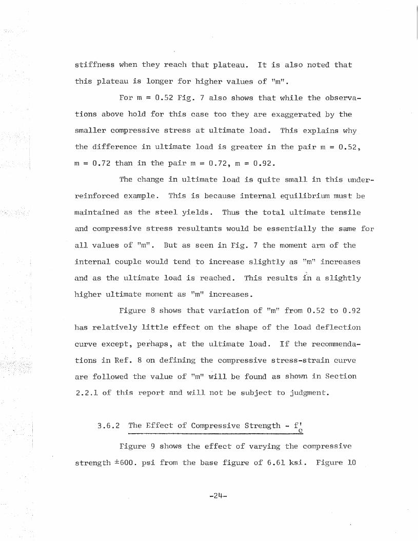
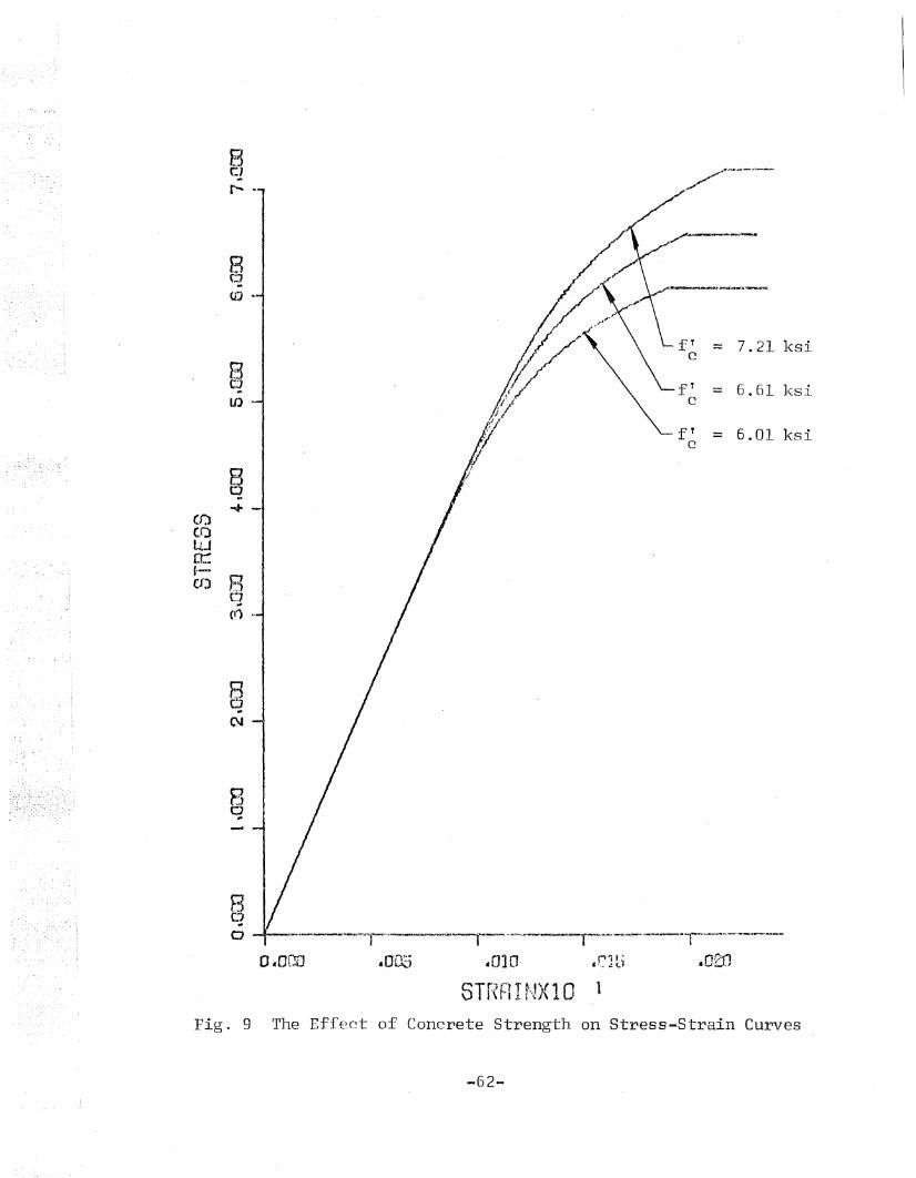
3.6.2 The Effect of Compressive Strength - fTc

Figure 9 shows the effect of varying the compressive

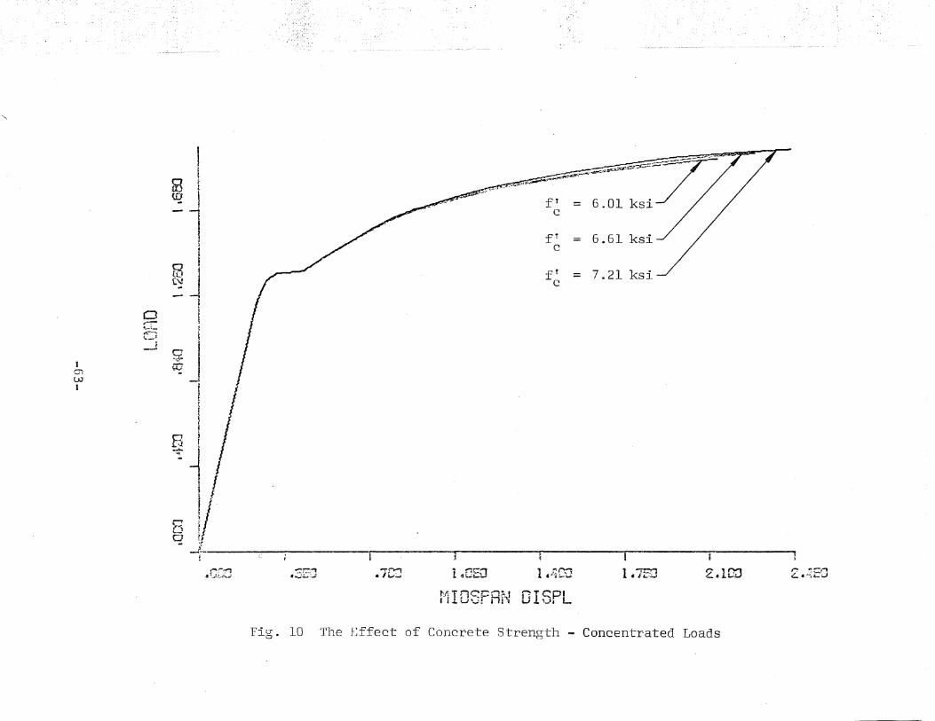
strength ±600. psi from the base figure of 6.61 ksi. Figure 10

-24--

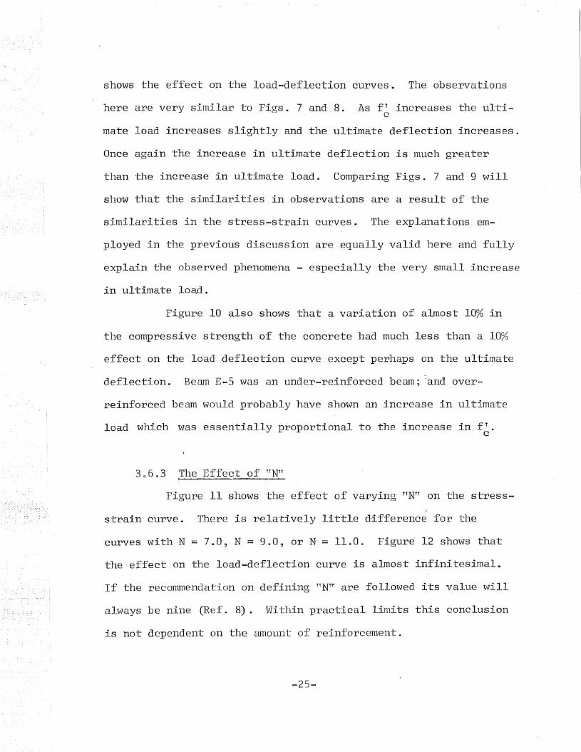
shows the effect on the load-deflection curves. The observations

here are very similar to Figs. 7 and 8. As £1 increases the ulti­c

mate load increases slightly and the ultimate deflection increases.

Once again the increase in ultimate deflection is much greater

than the increase in ultimate load. Comparing Figs. 7 and 9 will

show that the similarities in observations are a result of the

similarities in the stress-strain curves. The explanations em-

played in the previous discussion are equally valid here and fully

explain the observed phenomena - especially the very small increase

in ultimate load.

Figure 10 also shows that a variation of almost 10% in

the compressive strength of the concrete had much less than a 10%

effect on the load deflection curve except perhaps on the ultimate

deflection. Beam E-5 was an under-reinforced beam; :and over-

reinforced beam would probably have shown an increas:e in ultima·te

load which was essentially proportional to the increase in fT.C

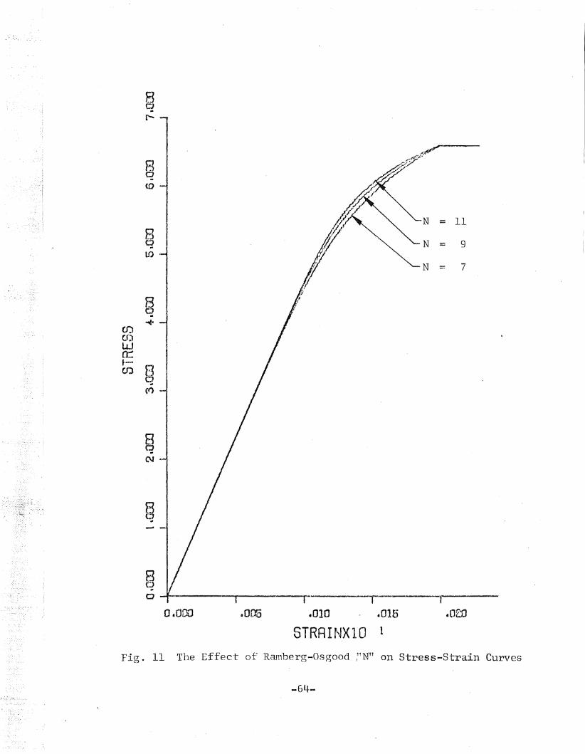
306.3 The Effect of TTNTT

Figure 11 shows the effect of varying TTNTT on the stress-/

strain curve. There is relatively little difference for the

curves with N = 7.0, N::: 9.0, or N::: 11.0. Figure' 12 shows that

the effect on the load-de.flection curve is almost infinitesimal.

If the recommendation on defining TTN'''' are followed its value will

always be nine (Ref. 8). Within practical limits this conclusion

is not dependent on the amount of reinforcement.

-25-

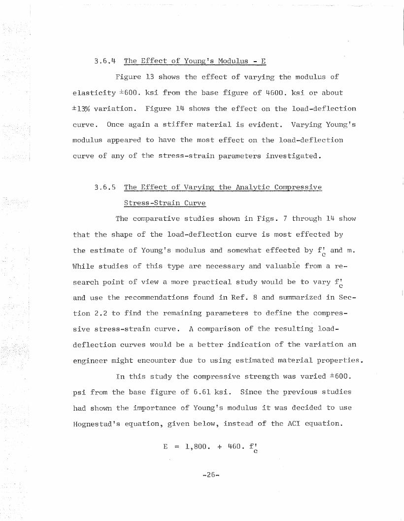
3.6.4 The Effect of YoungTs Modulus - E

Figure 13 shows the effect of varying the modulus of

elasticity ±600. ksi from the base figure of 4600. ksi or about

±13% variation. Figure 14 shows the effect on the load-deflection

curve. Once again a stiffer material is evident. Varying YoungTs

modulus appeared to have the most effect on the load-deflection

curve of any of the stress-strain parameters investigated.

3.6.5 The Effect of Varying the Analytic Compressive

Stress-Strain Curve

The comparative studies shown in Figs. 7 through 14 show

that the shape of the load-deflection curve is most effected by

the estimate of YoungTs modulus and somewhat effected by fT and m.c

While studies of this type are necessary and valuable from a re-

search point of view a more practical study would be to vary fTc

and use the recommendations found in Ref. 8 and summarized in Sec-

tion 2.2 to find the remaining parameters to define the compres-

sive stress-strain curve. A comparison of the resulting load-

deflection curves would be a better indication of the variation an

engineer might encounter due to using estimated material properties.

In this study the compressive strength was varied ±600.

psi from the base figure of 6~61 ksi. Since the previous studies

had shown the importance of YoungTs modulus it was decided to use

HognestadTs equation, given below, instead of the ACI equation.

E = 1,800. + 460. fTc

-26-

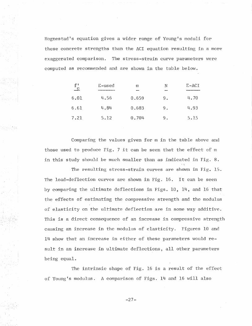
Hognestad's equation gives a wider range of YoungTs moduli for

these concrete strengths than the ACI equation resulting in a more

exaggerated comparison. The stress-strain curve parameters were

computed as recommended and are shown in the table below.

f1C

6.01

6.61

7.21

E-used

4.56

4.84

5.12

m

0.659

0.683

0.704

N

9.

9 •

9 ..

E-ACI

4.70

4.93

5.15

Comparing the values given for m in the table above and

those used to produce Fig. 7 it can be seen that the effect of m

in this study should be much smaller· than as indicated in Fig. 8.

The resulting stress-strain curves are shown in Fig. 15.

The load-deflection curves are shown in Fig. 16. It can be seen

by comparing the ultimate deflections in Figs. 10, 14, and 16 that

the effects of estimating the compressive strength and the modulus

of elasticity on the ultimate deflection are in some way additive.

This is a direct consequence of an increase in compressive strength

causing an increase in the modulus of elasticity. Figures 10 and

14 show that an increase in either of these parameters would re-

suIt in an increase in ·ultimate deflections, all other parameters

being equal.

The intrinsic shape of Fig. 16 is a result of the effect

of Young's modulus. A comparison of Figs. 14 and 16 will also

-27-

show that the extent of variation shown in Fig. 16 as almost one-

half that in Fig. 14e This is roughly the same as the extent of

change in YoungTs modulus corresponding to the two figures.

Figure 16 shows that, with the possible exception of

ultimate deflection, the effect of uncertainties inherent in engi-

neering estimates of material properties do not greatly alter the

resulting analytic load deflection behavior of a beam under in-

vestigation. This fact is in agreement with observed behavior of

test beams which are similar but not truly identical. While this

knowledge is necessary for confident usage of the computer program

it should not serve as an excuse for careless input.

3.7 The Effect of Tensile Stress Tolerance - rTOL

Figure 17 shows the result of varying the tolerance on

the tensile cracking strength from 1% to 10% to 2~~. The effect

is quite small and localized near the region of the load-deflection

curve corresponding to the rapid growth of cracking. The variation

of the tensile tolerance had the most profound and consistent ef-

feet on the execution speed of any parameter tested. Most para-

meters made little consistent difference but changing the tensile

tolerance from 1% to 20% reduced the execution time approximately

40%. This large change in computational effort is probably due to

a smaller number of load reductions required to meet the cracking

criterion. Each load reduction causes the original and well as

the ficticious loads to be resolvede This represents a considerable

-28-

effort each time the load reduction is necessary. In view of the

relatively small effect on the load-deflection curve produced by a

large tensile tolerance it would appear that using a large toler­

ance on preliminary studies should be considered as a cost reducing

factor~

308 The Effect of Tensile Strength - Ft

Figure 18 shows the effect of varying the tensile

strength of the concrete ±lOO. psi from the base value of 530. psi

which was already adjusted for dead, load tensile stress as indi­

cated in the discussion in Section 302.2 of Ref. 8. Figure 18

shows that the variation in tensile strength effects that region

of the load deflection curve at and beyond first cracking 0 The

increase in cracking load reflects the increase in tensile strength

as would be expected 0 The effect on the shape of the load­

deflection curve diminishes as the ultimate load is approached.

There is relatively little effect on the ultimate deflection or

ultimate load. The last two observations are consistent with the

discussion in Section 2.2 of Ref. 8 e

3.9 The Effect of Elemental Discretization

Figures 19 through 34 will be discussed separately and

in sub-groupso The 17 ft. 6 in. beam used in Se~tion 3.3 will

also be used here~ The areas of discussion are:

-29-

10 The effect of the total number of elements on the load­

deflection behavior.

2. The effect of the total number of elements on the con­

verged solution in the linear elastic region.

3. The effect of the total number of elements on the con­

verged solution in the nonlinear region.

4. The effect of the type elemental discretization, i.e.

the position of the small element, on all of the above.

Figure 19 shows the elemental discretization used. The

example number used to keep track of the various computer execu­

tions will be used in the discussion to distinguish the various

examples. As shown, the three figures in Fig. 19 will be con­

sidered as TT r ightT1 for some examples because the centerline of the

beam will be on the right side of each sketch. The simple support

will be on the left. Symmetry was used in these examples. Some

of the test examples were TTleft TT, that is to say that the center­

line of each sketch in Fige 19 is now on the left and the support

is on the right. The obvious difference is the location of the

small element in each case. The various example numbers are shown

in the table below.

-30-

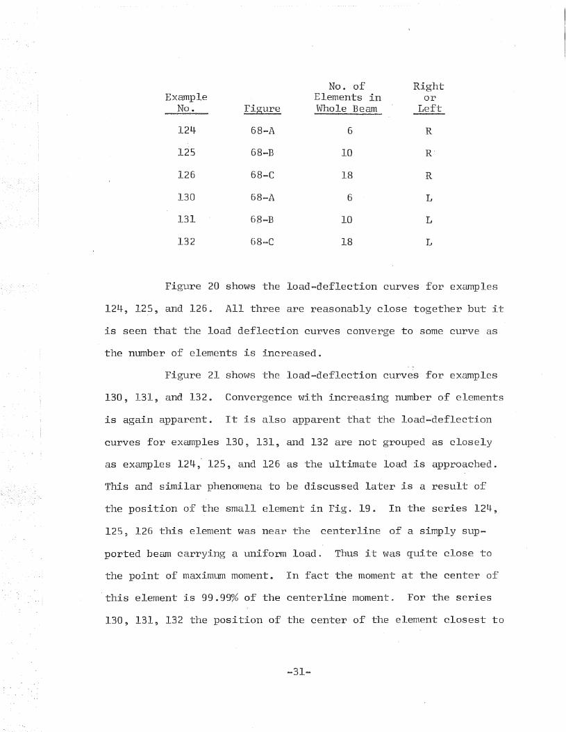
No. of RightExample Elements in or

No. Figure Whole Beam Left

124 68-A 6 R

125 68-B 10 R'

126 68-C 18 R

130 68-A 6 L

131 6S-B 10 L

132 68-C 18 L

Figure 20 shows the load-deflection curves for examples

124, 12?, and 126. All three are reasonably close together but it

is seen that the load deflection curves converge to some curve as

the number of elements is increased.

Figure 21 shows the load-deflection curves for examples

130, 131, and 132. Convergence with increasing number of elements

is again apparent. It is also apparent that the load~deflection

curves for examples 130, 131, and 132 are not grouped as closely

as examples 124, 125, and 126 as the ultimate load is approached.

This and similar phenomena to be discussed later is a result of

the position of ~he small element in Fig. 19. In the series 124,

125, 126 this elerrlent was near the centerline of a simply sup-

ported beam carrying a uniform load. Thus it was quite close to

the point of maximum moment. In fact the moment at the center of

'this element is 99.99% of the centerline moment. For the series

130, 131, 132 the position of the center of the element closest to

-31-

the centerline reached moments of 93.9%, 98.5, and 99.6% of the

centerline moment respectively. This position at which stress is

measured results in increased predicted values of cracking load, as

seen in the printed output,and ultimate load. There is also a de­

lay in the initiation and progression of inelastic actions. The

computed ultimate loads for examples 130, 131, and 132 have the

ratios 1.088, 1.014, and 1.000 compared to the moment ratios from

the percentages of centerline moment of 1.061, 1.011, and 1.000.

Thus the position of the point where stress is measured (the layer

centroid) accounts for most of the range of ultimate loads. Ele­

mental discretization probably accounts for the rest. The range

of ultimate deflections is probably also influenced by the geomet­

ric factors of slope at the most stressed element and the distance

from its layer centroid to the centerline node.

Figure 20 shows that the small element near the center­

line produced a much smaller range of ultimate loads and ultimate

deflections. The ultimate load ratios were 0.999, 0.997, and

1.000 based on example 126. These values are so close that the

approximations inherent in the numerical solution of nonlinear

problems precludes any conclusions as to the crudest discretiza­

tion, example 124, having a 1Tcloserr1 ultimate load than example 125.

Comparison of the elastic range of Figs. 20 and 21 show

that the effect of the number of elements is quite small in that

range. The effect appears to increase as nonlinear behavior pro­

ceedsa These figures show that both types of discretization

-32-

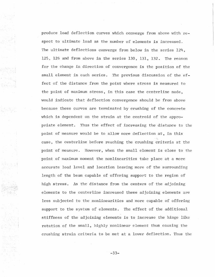
produce load deflection curves which converge from above with re-

spect to ultimate load as the number of elements is increased.

The ultimate deflections converge from below in the series 124,

125, 126 and from above in the series 130, 131, 132. The reason

for the change in direction of convergence is the position of the

small element in each series. The previous discussion of the ef-

feet of the distance from the point where stress is measured to

the point of maximum stress, in this case the centerline node,

would indicate that deflection convergence should be from above

because these curves are terminated by crushing of the concrete

which is dependent on the strain at the centroid of the appro-

priate element. Thus the effect of increasing the distance to the

point of measure would be to allow more deflection at, in this

case, the centerline before reaching the crushing criteria at the

point of measure. However, when the small element is close to the

point of maximum moment the nonlinearities take place at a more

accurate load level and location leaving more of the surrounding

length of the beam capable of offering support to the region of

high stress. As the distance from the centers of the adjoining

elements to the centerline increased these adjoining elements are

less subjected to the nonlinearities and more capable of offering

support to the system of elements. The effect of the additional

stiffness of the adjoining elements is to increase the hinge like

rotation of the small, highly nonlinear element thus causing the

crushing strain criteria to be met at a lower deflection. Thus the

-33-

deflection of the beam is reduced and deflection convergence is

from below as the number of elements is increased and the small

element is kept near the point of maximum moment.

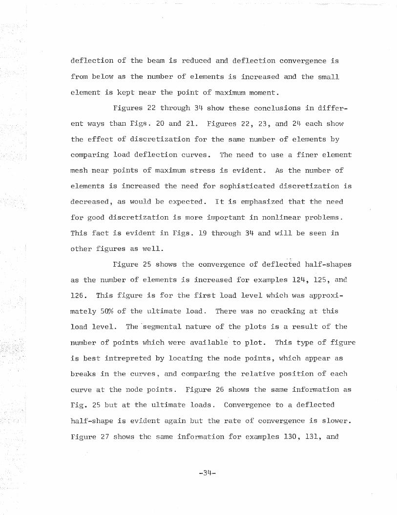
Figures 22 through 34 show these conclusions in differ­

ent ways than Figs. 20 and 21. Figures 22,- 23, and 24 each show

the effect of discretization for the same number of elements by

comparing load deflection curves. The need to use a finer element

mesh near points of maximum stress is evident. As the number of

elements is increased the need for sophisticated discretization is

decreased, as would be expected. It is emphasized that the need

for good discretization is more important in nonlinear problems.

This fact is evident in Figs 0 19 through 34 and will be seen in

other figures as well.

Figure 2S shows the convergence of deflected half-shapes

as the number of elements is increased for examples l2~, 125, and

126. This figure is for the first load level which was approxi­

mately 50% of the ultimate load. There was no cracking at this

load level. The 'segmental nature of the plots is a result of the

number of points which were available to plot. This type of figure

is best intrepreted by locating the node points, which appear as

breaks in the curves, and comparing the relative position of each

curve at the node points. Figure 26 shows the same information as

Fig. 25 but at the ultimate loads. Convergence to a deflected

half-shape is evident again but the rate of convergence is slower.

Figure 27 shows the same information for examples 130, 131, and

-34-

132 as Fig. 25 did for examples 124, 125, and 126. Likewise Fig.

28 is analogous to Fig. 26.

Figures 29 to 34 show the effect of discretization.

Figure 29 shows the deflected half-shape of examples 124 and 130.

The effect of the location of the small element is again apparent.

This figure and Figs. 30 and 31 show conditions at the ultimate

load. Figure 30 shows the same information as Fig. 29 for ex­

amples 125 and 131. Figure 31 applies to examples 126 and 132.

Consideration of the last three figures as a group shows again

that as the number of elements increases the need for sophisti­

cated discretization decreases and that an adequate number of ele­

ments and a sensible discretization are necessary when nonlinear

problems are attacked.

Figures 32 to 34 show the same information as Figs. 29

to 31 except that they apply to a load level which is still linear.

They show that, for linear response and for this application, the

effect of discretization is quite small. It is noted that in

this application 'there were no extreme stress gradients and that

the shape function used here is a conforming shape function (Ref.

11). The conclusion about discretization in the linear range

should not be generalized beyond this application to beams. The

conclusion that more care is necessary in discretising a region

for a nonlinear problem appears to be general.

The loads for which Figs. 32 to 3~ are plotted were

slightly different. This difference is small but since each pair

-35-

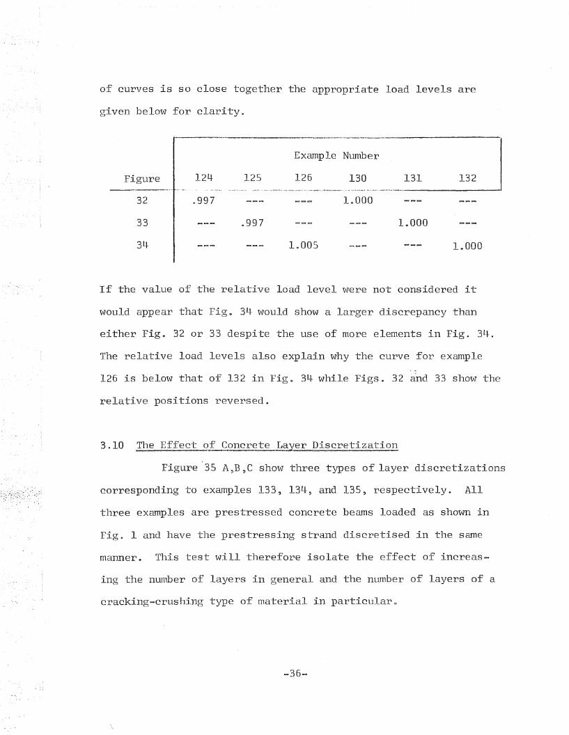
of curves is so close together the appropriate load levels are

given below for clarity A

Example NillTIber

Figure 124 125 126 130 131 132

32 .997

33

34

.,997

1.005

1.000

1.000

If the value of the relative load level were not considered it

would appear that Fige 34 would show a larger discrepancy than

either Fig. 32 or 33 despite the use of more elements in Fig. 34.

The relative load levels also explain why the curve for example

126 is below that of 132 in Fig. 34 while Figs. 32 and 33 show the

relative positions reversed.

3.10 The Effect of Concrete Layer Discretization

Figure 35 A,B,C show three types of layer discretizations

corresponding to examples 133, l3~, and 135, respectively. All

three examples are prestressed concrete beams loaded as shown in

Fig. 1 and have the prestressing strand discretised in the same

manner. This test will therefore isolate the effect of increas-

ing the number of layers in general and the number of layers of a

cracking-crushing type of material in particularo

-36-

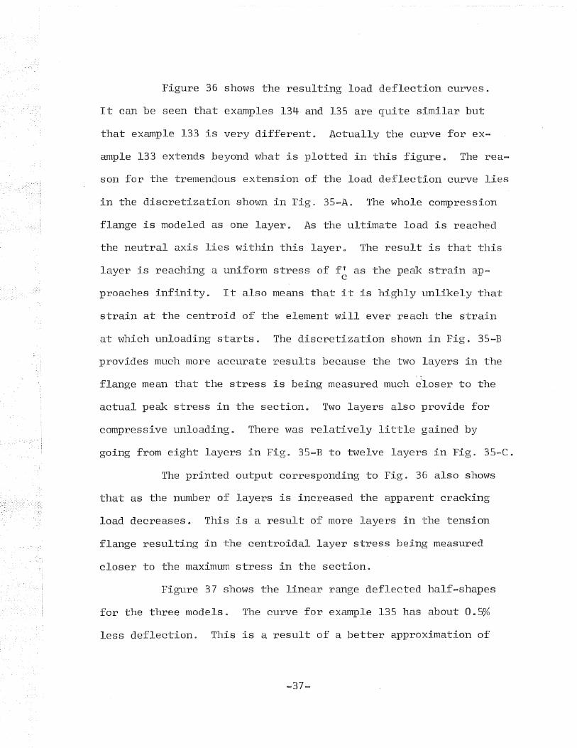
Figure 36 shows the resulting load deflection curves.

It can be seen that examples 134 and 135 are quite similar but

that example 133 is very different. Actually the curve for ex-

ample 133 extends beyond what is plotted in this figure. The rea-

son for the tremendous extension of the load deflection curve lies

in the discretization shown in Fig~ 35-AQ The whole compression

flange is modeled as one layer. As the ultimate load is reached

the neutral axis lies within this layer@ The result is that this

layer is reaching a uniform stress of fT as the peak strain ap­e

proaches infinity 0 It also means that it is highly unlikely that

strain at the centroid of the element will ever reach the strain

at which unloading starts. The discretization shown in Fig. 35-B

provides much more accurate results because the two layers in the. ~

flange mean that the stress is being measured much closer to the

actual peak stress in the section. Two layers also provide for

compressive unloading a There was relatively little gained by

going from eight layers in Figa 35-B to twelve layers in Fig. 35-Ce

The pri'nted output corresponding to Fig e 36 also shows

that as the number of layers is increased the apparent cracking

load decreases., This is a result of more layers in the tension

flange resulting in the centroidal layer stress being measured

closer to the maximum stress in the sectionD

Figure 37 shows the linear range deflected half-shapes

for the three models. The curve for example 135 has about 0.5%

less deflection~ This is a result of a better approximation of

-37-.

the moment of inertia of the trapazoidal section of the I-beam by

the two layers as shown in Fig. 35-C.

Figure 38 shows the deflected half-shapes at ultimate

loads for examples 134 and 135 and a selected curve for example

133$ It can be seen that there is a somewhat larger difference in

examples 134 and 135 at ultimate load than in the linear case.

This is to be expected. Again, numerical aspects have to be con­

sidered when drawing conclusions from results which are so close

together. It appears reasonable to conclude that as the number of

layers increases the solutions converge to some deflected shape,

especially if the additional layers are added with judgment. It

should be apparent that, from a strict consideration of the number

of layers, dividing the bottom flange of the beam in Fig. 35-A into

ten layers would have almost no effect on the results of example

133 as the ultimate load is approached. It might, however result

in a more realistic speed of release of the strain energy from

cracking. This would be minimized by the fact that the cracking

extended far above the bottom flange at ultimate load. In this

context the result of better layering of the tensile flange

reaches a point of diminishing returns.

3.11 The Effect of Reinforcement Discretization

Figure 39 shows the effect of discretization of the pre­

stressing strands of the load-deflection curve. Example 102 had

three rows of strand corresponding to the three rows shown in Fig.

-38-

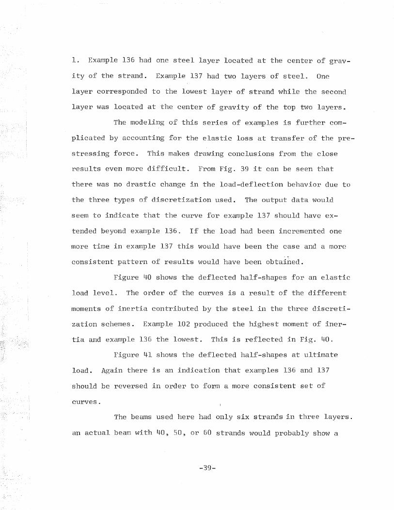
l~ Example 136 had one steel layer located at the center of grav­

ity of the strand. Example 137 had two layers of steel. One

layer corresponded to the lowest layer of strand while the second

layer was loqated at the center 6f gravity of the top two layers.

The modeling of this series of examples is further com­

plicated by accounting for the elastic loss at transfer of the pre­

stressing force. This makes drawing conclusion~ from the close

results even more difficult. From Fig. 39 it can be seen that

there was no drastic change in the load-deflection behavior due to

the three types of discretization used. The output data would

seem to indicate that the curve for example 137 should have ex­

tended beyond example 136. If the load had been incremented one

more time in example 137 this would have been the case and a more

consistent pattern of results would have been obtained.

Figure 40 shows the deflected half-shapes for an elastic

load level. The order of the curves is a result of the different

moments of inertia contributed by the steel in the three discreti­

zation schemes. Example 102 produced the highest moment of iner­

tia and example 136 the lowest. This is reflected in Fig. 40.

Figure 41 shows the deflected half-shapes at ultimate

load. Again there is an indication that examples 136 and 137

should be reversed in order to form a more consistent set of

curves.

The beams used here had only six strands in three layers.

an actual beam with 40, 50, or 60 strands would probably show a

greater range of results. Secondary effects due to stress concen-

trations around the strand, crack arresting and similar effects

are beyond the scope of this analysis. Computer printed plots

showing the stress field and the growth of cracks did indicate

that example 136 produced faster crack growth than example 137

which was, in turn, faster than 102. These results probably re-

fleet the more accurate modeling of moment of inertia contributed

by the strand.

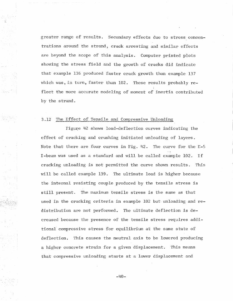
3.12 The Effect of Tensile and Compressive Unloading

Figu~e 42 shows load-deflection curves indicating the

effect of cracking and crushing initiated unloading of layers.

Note that there are four curves in Fig. 42. The curve for the £-5

I-beam was used as a standard and will be called example 102. If

cracking unloading is not permitted the curve shown results. This

will be called example 139. The ultimate load is higher because

the internal resisting couple produced by the tensile stress is

still present. The maximum tensile stress is the same as that

used in the cracking criteria in example 102 but unloading and re-

distribution are not performed. The ultimate deflection is de-

creased because the presence of the tensile stress requires addi-

tional" compressive stress for equilibrium at the same state of

deflection. This causes the neutral axis to be lowered producing

a higher concrete strain for a given displacement. This means

that compressive unloading starts at a lower displacement and

-40-

results, eventually, in a failure to converge. Looked at another

way, the difference in displacement results from the redistribution

of stresses after cracking. The loss of elemental stiffness is

the same in both cases.

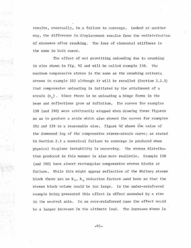
The effect of not permitting unloading due to crushing

is also shown in Fig. 42 and will be called example 138. The

maximum compressive stress is the same as the crushing criteria

stress in example 102 although it will be recalled (Section 2.2.1)

that compressive unloading is initiated by the attainment of a

strain (81

) a Since there is no unloading a hinge forms in the

beam and deflections grow ad infinitum. The curves for examples

138 (and 140) were arbitrarily stopped when drawing these figures

so as to produce a scale which also showed the curves for examples" .

102 and 139 to a reasonable size. Figure 42 shows the value of

the downward leg of the compressive stress-strain curve; as stated

in Section 2.3 a numerical failure to converge is produced when

physical in-plane instability is occurring. The stress distribu-

tioD produced in this manner is "also more realistic. Example 138

(and 140) have almost rectangular compressive stress blocks at

failure. "While this might appear reflective of the Whitney stress

block there are no k 1 , k3

reduction factors used here so that the

stress blocl< volume could be too large. In the under-reinforced

example being presented this effect is offset somewhat by a rise

in the neutral axis. In an over-reinforced case the effect would

be a larger increase" in the ultimate load. The increase shown in

-41-

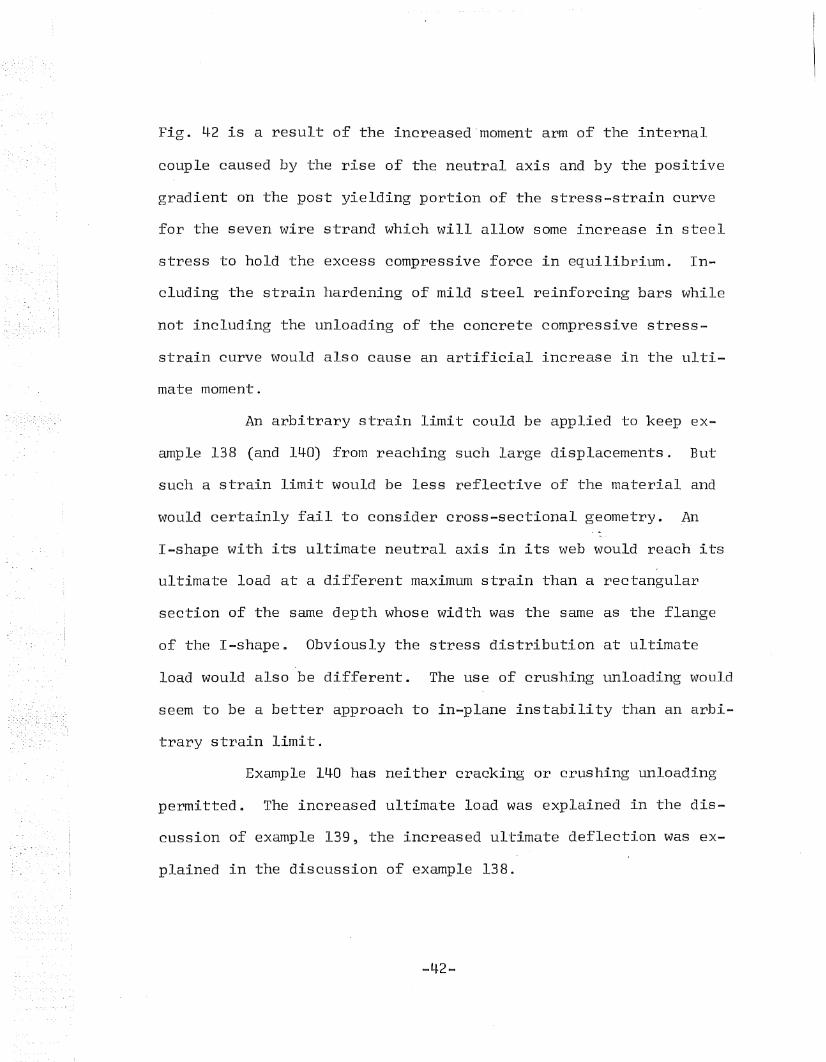
Fig. 42 is a result of the increased'moment arm of the internal

couple caused by the rise of the neutral axis and by the positive

gradient on the post yielding portion of the stress-strain curve

for the seven wire strand which will allow some increase in steel

stress to hold the excess compressive force in equilibrium. In-

eluding the strain hardening of mild steel reinforcing bars while

not including the unloading of the concrete compressive stress-

strain curve would also cause an artificial increase in the ulti-

mate moment.

An arbitrary strain limit could be applied to keep ex-

ample 138 (and 140) from reaching such large displacements. But

such a strain limit would be less reflective of the material and

would certainly fail to consider cross-sectional geometry. An

I-shape with its ultimate neutral axis in its web would reach its

ultimate load at a different maximum strain than a rectangular

section of the same depth whose width was the same as the flange

of the I-shape. Obviously the stress distribution at ultimate

load would also be different. The use of crushing unloading would

seem to be a better approach to in-plane instability than an arbi-

trary strain limit.

Example 140 has neither cracking or crushing unloading

permitted. The increased ultimate load was explained in the dis-

cussion of example 139, the increased ultimate deflection was ex-

plained in the discussion of example 138.

-42-

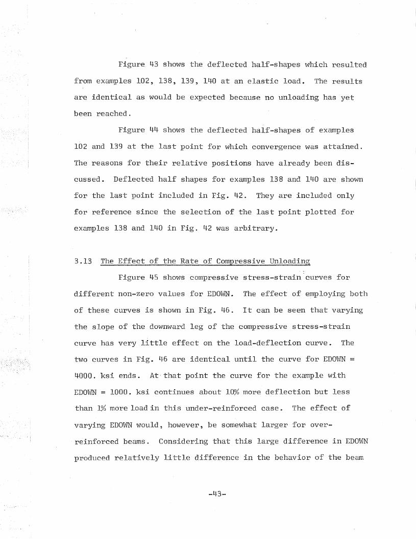
Figure 43 shows the deflected half-shapes which resulted

from examples 102, 138, 139, 140 at an elastic load. The results

are identical as would be expected because no unloading has yet

been reached.

Figure 44 shows the deflected half-shapes of examples

102 and 139 at the last point for which convergence was attained.

The reasons for their relative positions have already been dis-

cussed. Deflected half shapes for examples 138 and 140 are shown

for the last point included in Fig. 42. They are included only

for reference since the selection of the last point plotted for

examples 138 and 140 in Fig. 42 was arbitrary.

3.13 The Effect of the Rate of Compressive Unloading

Figure 45 shows compressive stress-strain curves for

different non-zero values for EDOWN. The effect of e~ploying both

of these curves is shown in Fig. 46. It can be seen that varying

the slope of the downward leg of the compressive stress-strain

curve has very little effect on the load-deflection curve. The

two curves in Fig. 46 are identical until the curve for EDOWN =

4000. ksi ends. At-that point the curve for the example with

EDOWN = 1000. ksi continues about 10% mor'e deflection but less

than 1% more load in this under-reinforced case. The effect of

varying EDOWN would, however, be somewhat larger for over-

reinforced beams. Considering that this large difference in EDOWN

produced relatively little difference in the behavior of the beam

-43-

it would appear that the values for EDOWN given in Table I of Ref.

8 can be used with confidence. The conclusion here ,that varying

the value of EDOWN does not greatly effect the load deflection

curves in this case does not negate the previous conclusions about

the need for a non-zero downward slope for cracking or crushing

analysis.

A parametric study relative to the effect of EDOWNT, the

rate of tensile unloading, was included in Section 2.2 of Ref. 8.

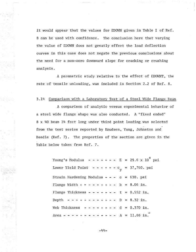
3.14 Comparison with a Laboratory Test of a Steel Wide Flange Beam

A comparison of analytic versus experimental behavior of

a steel wide flange shape was also conducted. A TTfixed ended"

8 x 40 beam 14 feet long under third point loading was selected

from the test series reported by Knudsen, Yang, Johnston and

Beedle (Ref. 7). The properties of the section are given in the

Table below taken from Ref. 7.

Yqung's Modulus6- - - - - - - E = 29.6 x 10 psi

Lower Yield Point - - - - - - a = 37,760. psiy

Strain Hardening Modulus - - - c = 630. psi

Flange Width - - - - - - - - - b = 8.06 in.

Flange Thickness - - - t = 0.552 in.

Depth - - - - - - - - D = 8.32 in.

Web Thickness d = 0.370 in.a

Area - - - - - - - - - - - A = 11.66 in.

-4-4-

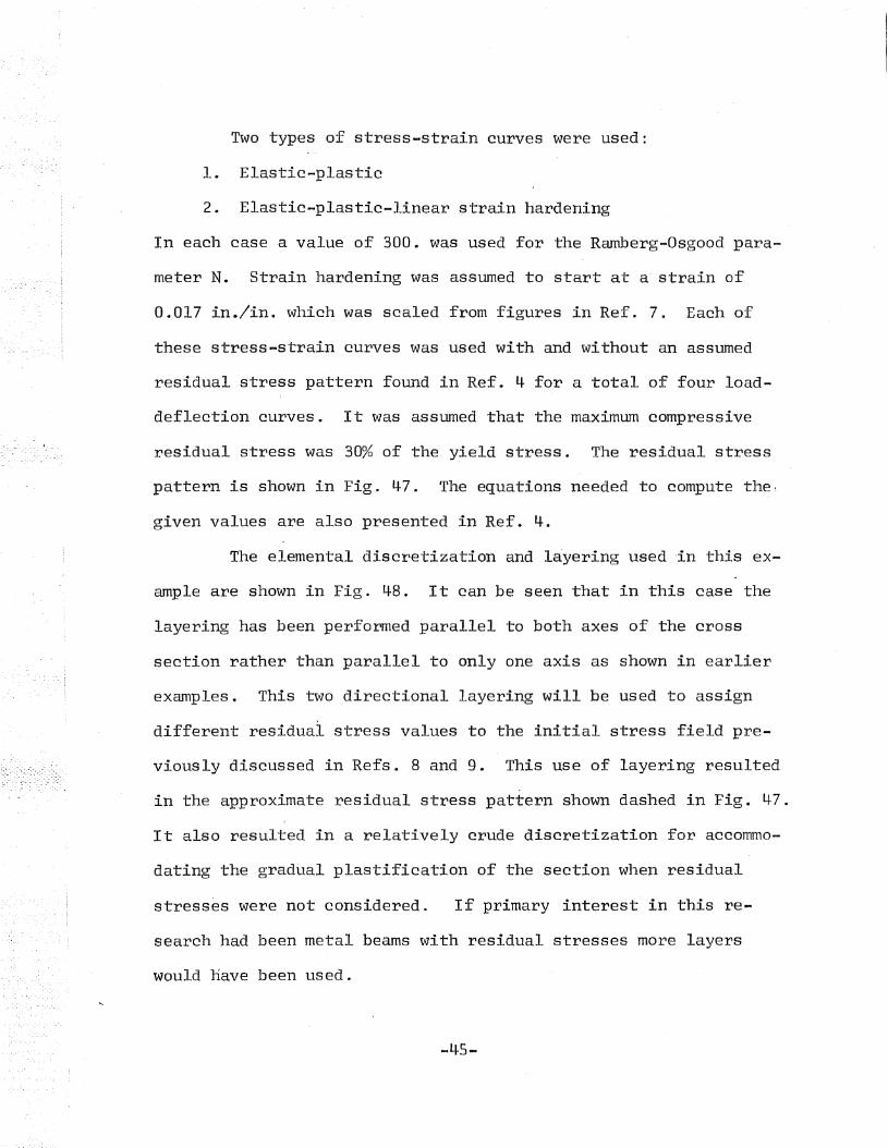
Two types of stress-strain curves were used:

1. Elastic-plastic

2. Elastic-plastic-linear strain hardening

In each case a value of 300. was used for the Ramberg-Osgood para­

meter N. Strain hardening was assumed to start at a' strain of

0.017 in./in. which was scaled from figures in Ref. 7. Each of

these stress-strain curves was used with and without an assumed

residual stress pattern found in Ref. 4 for a total of four load­

deflection curves. It was assumed that the maximum compressive

residual stress was 30% of the y~eld stress. The residual stress

pattern is shown in Fig. 47. The equations needed to compute th~~

given values are also presented in Ref. 4.

The elemental discretization and layering used ,in this ex­

ample are shown in Fig. 48. It can be seen that in this case the

layering has been performed parallel to both axes of the cross

section rather than parallel to only one axis as shown in earlier

examples. This two directional layering will be used to assign

different residual stress values to the initial stress field pre­

viously discussed in Refs. 8 and 9. This use of layering resulted

in the approximate residual stress pattern shown dashed in Fig. 47.

It also resulted in a relatively crude discretization for accommo­

dating the gradual plastification of the section when residual

stresses were not considered. If primary interest in this re­

search had been metal beams with residual stresses more layers

would have been used.

-45-

The individual layers could also have been assigned

separate stress-strain curves to try to account for the change in

strain at the onset of strain hardening caused by the residual

stresses. This was not actually done and any attempt to do so

would have been an .approximation.

The four load deflection curves resulting from the com.­

bination of stress-strain curves with and without residual stresses

is shown in Fig. ~9. Also shown is the experimental load deflec­

tion curve and the results obtained by nwnerical integration of

the distribution of curvature along the beam. This numerical in­

tegration scheme is said to be theoretically exact (Ref. 7)~ but

its application involves a trial and error numerical scheme so

that some error is to be expected. The numerical integration

scheme also included strain hardening but did not include residual

stresses. It can be seen that while there were only seven numeri­

cal integration points given they agree quite well with the strain

hardening results presented here. It can also be seen that the

experimental and' analytic results differ significantly between de­

flections of about 0.3 inches to about 0.9 inches. This differ­

ence reaches about 7~~ at a displacement of about 0.4 inches but

is less over the rest of the range. There are several reasons for

this discrepancy:

1. The TTfixed end TT of the beam was framed into a su,pporting

connection which was not perfectly rigid. During this

-46-

test series several support condit~ons were tried and

this particular specimen had the most end rigidity.

2. The residual stress pattern assumed is only approximately

representative of wide flange beams. The welding re­

quired at the TTfixed ends TT would change the residual

stress pattern drasticallyo

3. As previously mentioned, the layering used was relatively

crude, although experience would indicate that, this would

be a minor source of error.

Knudsen et al. made several references to the residual

stress in the TTaS deliveredTT beams and indicated that this was a

large source of error in comparisons with their calculations~ Re­

ference to Fig. 49 shows that the compensation offered by the as­

sumed residual stress pattern is reasonable as/plastification

reaches the pure moment section of the byam. It also suggests

that a higher le~el of residual stresses than that assumed is in­

dicated. Plastification of the TTfi:x.ed ends TT, however, shows rela­

tively little effect of the assumed residual stresses indicating

that the welding in that area and the lack of total fixity are

large factors in the apparent discrepancy.

The simple plastic theory would predict a collapse load._

of 107. kips for this beam. The elastic-plastic stress-strain

curve with N = 300. yielded the following results without residual

stresses.

-47-

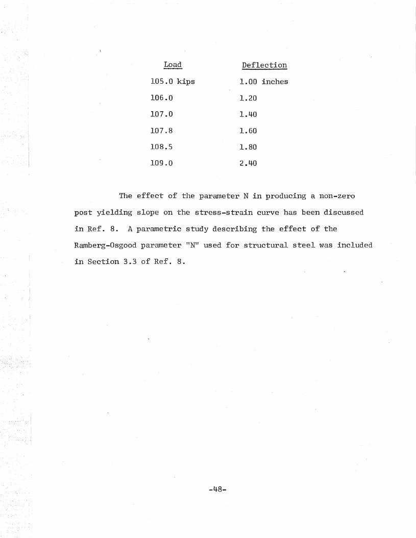
Load Deflection

105.0 kips 1.00 inches

106.0 1.20

107 .0 1.40

107.8 1.60

108.5 1.80

109.0 2.40

The effect of the parameter N in producing a non-zero

post yielding slope on the stress-strain curve has been discussed

in Ref. 8. A parametric study describing the effect of the

Ramberg-Osgood parameter TTNTT used for structural steel was included

in Section 3.3 of Ref. 8.

-48-

4. CONCLUSIONS FROM THE PARAMETRIC STUDY

4.1 Iteration Tolerance

This method is relatively insensitive to the iteration

tolerance,.· Since at least two] iterations will be needed for each

load step the results should, theoretically, be better. than a

non-iterative method which would be approached as the iteration

tolerance increased. This assumes that the same size load steps

would be used.

4.2 Yield Point of Prestressing Strand, Draped Strand

and Uniform Loads

The method gives logically defendable results for such

conditions other than those used for comparisons in Ref. 8 as in-

creasing the yield point of the prestressing strand, using draped

strand or a uniform load. This last condition was compared with

results of laboratory tests in this report.

4.3 Stress-Strain Curve Parameters

The load-deflection curves of under-reinforced concrete

beams was seen to be effected by the concrete compression curve

parameters in the following manner.

a)

b)

c)

E and fT caused the most change.c

m caused less but still significant changes.

N caused almost no change.

-49-

These conclusions could also be extended to over-reinforced beams

by modifying the stiffer. material concept to include the fact that

stiffer materials would in general increase the ultimate strength

of over-reinforced beams.

4.4 Effect of Estimating Material Properties

The normal uncertainties about material properties do

not render the method ineffective. Inaccurate material assump­

tions will have the most effect on calculated ultimate deflections

in under-reinforced beams.

4.5 Tensile Tolerance

The tensile tolerance has the most significant and con­

sistent effect on execution speed of the program.

4.6 Elemental Discretization

a) As the number of elements increases the load-deflection

curves converge to some curve. Good discretization speeds

the convergence to this curve but its effect decreases as

the number of elements increases.

b) Sophisticated discretization can lead to improved results

all the way along the nonlinear portion of the load­

deflection curve. Note the effect of the position of the

small element in Section 3.9.

-50-

c) In general, the use of fewer elements causes an over­

estimation of the ultimate load although good discreti­

zation can reduce the error considerably.

d) The direction of convergence to ultimate deflection is

dependent on the type of discretization.

e) This method of analysis for beams gives good results in

the linear range even when very few elements are used.

4.7 Number of Layers

In general, the use of more layers improves the results

but good results can be obtained with a few well placed layers.

Care must be taken that the ultimate neutral axis not fall within

the only remaining uncracked layer. In the linear range the solu­

tion is independent of the number of elements as long as the pro­

perties defining the elasticity matrix are correct.

4.8 Cracking and Crushing Induced Stress Unloading

Tensile unloading is necessary for an accurate load­

deflection curve. A better physical representation of the beam

or beam-column as well as improved stresses and a simulation of

in-plane instability result if compressive unloading is also used.

In over-reinforced beams, not including compressi,ve unloading

would overestimate the ultimate load.

-51-

4.9 Steel Wide Flange Beam

This method of analysis is also valid for steel beams

until local or lateral torsional buckling occur. The effects of

residual stresses and strain hardening can also be included if

parameters which define them can be determined.

4.10 General Comments

As with all numerical analysis it is difficult to gen­

eralize the results of this type of parametric study with absolute

confidence. Rather, information of this type should be considered

as a guide. It is possible that some example could be devised

which would refute almost anyone of the conclusions.

-52-

5. FIGURES

-53-

a.. ,a

V~ lV

-~

A .#

Elevation

3854 in,4 3986 in.4

1l·28.2 In.'' 450.9 in.:) -J262.5in.3 2-10.9 in.::> I

AIzt

Qcg

Qbf

ZbQtf

Section PropertiesConcrete T-r-a·-n-sf-~o-rm-l-e-d---;

Property Section I Section 2

102.0 in.2 IC)5.3 in.2

t

Section A-A

7/16 Strand Typ.4-1/211 4-1/2"

9 11.

-- I

3":..:::::::.::::t

- iL tf 2u

co

~¢II,

- 311 .r: lJ :211.. . I ;:)

3"-0 \lI ~.

- 8"j

~g2 [~ i~15-3/411bf

cgs /' _~1-3/4~ 211

/' -t

t

311-r= -'(~ilb J"T

T J L1-1/2"II

¢coro

Fig. 1 Properties of Prestressed Concrete I-Beams

-54-

2 ~ J1~:G

I -1 --1

1 (11 00 l t 75fJ 2 ~ 1CO

_~>c~.,-.-

1 ,CEO

----r--(JE5CJ c 700(ooc

CJ[~)

o

C::.l:n(\..1

I!

Q~l,. ... J

'n\---

II

Ii

1I

I IC"'I1tr( -,',

:1~~ J

1

I!

CJCl~

o--l

IU1lf11

~!1T nSPc)~JI.... u.,..JJ '\J r~T:""'PLU.I..J; _

Fig. 2 The Effect of Iteration Tolerance - Concentrated Loads

IU1enI

oo<.C''-:l

1j!

o I

~~

u Io I

---l 0 Ilj

if~ II

RL ....'!

~.

/

'/pi

1///

j/i/

/I!

o

~----­~~--

~~-~-_?'

~~/

Analytic

Experimental

.-------

:600

o I'. -- I1.J,.:.., -\......I

1 I I I

~OOO l~JOO (QeDr1 e200

1-- I

1c5CO 1c800 241 eel

MID5PRN OI5PLFig. 3 Load-Deflection Curves - Uniform Load

•.-;:;:.---=:;:;.-

~~~~

EDOWNT = 20,000 ksi

~J

I

-'"...

, /~/

P/:::;:://

./-//'

//'/

EDOWNT = 800 ksi

CJCoJC

,000 (1riO ,320 .n. ~-:'r'"t I..JU (R40 ((30C t9BO i ,12e

MI 05PR~'1J 0T5PL

Fig. 4 The Effect of Tensile Unloading Rate - Uniform Load

Il

ji

I

I

11/ji

8to

-=1t

i!

~ \Lf = 265 ksi~

8 I(\:

--i r L-f = 225 ksi

Ij

Qt._)(A..!

8~-

8o

--'

o,,';-'-.....~.~

oIlJ100I

I~--- I --f-~---~-~l--~-----~~---! t I i

.oon .1m .soo 4.420 e6m .750 .9.00 1.CED(\.A "!" n:""'"\~~l\ 1 0I L"r-:.rfi 1 Ljurr-if'J ~'J·rL

Fig. 5 The Effect of Steel Yield Stress - Uniform Load

r.~

(,\_....

~-5

~~

--- --------------------------------.....-----~

Straight Strand

Draped Strand

-------T----------------·'r-------------r-----·--------r--·----·-·--·---·+··-·\

....,~ ~~~

.... ~ ~

,1

Ii

\1 Il~-..c"\

.l.,.~

~o I

JI r[ /./! ,/

I,/'

//~

'I f---------- .-// //

I ! /'-1 ,r! II ;/

o I-d-. !(.:".] !

~ /I /I I

c I ;1C"J"!

1/~

I

j

.---J

L~G~

CJ

IlJ1lDI

~c[JG t:3EG ~7CG 1 (:~T:J:J 1 r:nr_ ~4UJ 1 ,)fjC; 2. j CC~ ~) _.'2: ~c

tvl T r-~; (~~.pc_~ f'll r; Tc:: P Lj! J_U\......... I 1.;\ L..- ~\.•). ~

Fig. 6 The Effect of Draped Strand - Concentrated Loads

'~-""---

0.52

8 m = 0.72(:]LD ., m == 0.92

Bq

8r.J(0"'"

f3Sfo -"--"'--"'-~""--""--"'~'''''''''''-''---~.'r------r''''''-''''

cOG] .005 .012 .018

S1'RFl I f\JX 10 1

8<:1~

Fig. 7 TIle Effect of Ramberg-Osgood 1T m'1 on Stress-Strain Curves

-60-

JUlf-IJ

~l--j

II

8 I'-"f J

~1g I0_ ~

o i--1 j

~Ji

I~1

I

8o

~~4.i-r-L::":...J .3EO .7w 1cOw

m

m = o. 72

m = 0.92

1 ,400 1.7ED 24!lCJ 2e4C0

r1 I DSPAf\l 0ISPL

Fig. 8 The Effect of Ramberg-Osgood TTmTT - Concentrated Loads

= 7.21 ksi

= 6.61 l<si

f t = 6.01 ksic

8o~

BC]o ..·-----''''''''"'r'"'-....- ........''''..-...--r-----~ .......'---·--T-·"'.....,.,.·---..----·-1-·-...."' ...-'-----

0.000 .O~) .010 .C}G .020

STf<FI I f\J}( 10

8o-+-

8C1

<D-

8-olD-

(f)(ljwtr:~f) B(1

(f') ."

Fig. 9 The Effect of Concrete Strength on Stress-Strain Curves

-62-

'''.

f f = 7.21 ksic

fT =6.61ksic

_- _.,"-" ..~"'-'---A;---."'".;.dr~'.,:::;~;;:....7/-~....:::;;....-~-,·-· ....·"

fT - /c - 6.01 ksi

"::'7:::1.-'~~J..G~:0

Ifti ~I·fJ:!.

-lt

If3 1L:! J- i

I~

ig I~J

i!t

!tf

R;

'! ~ /

81;'o !

~.-----------'r-f-----..,r-I-------r~-----':-I----~J----~!

.7CJ 1 aOSJ 1 c~~m 1.7EO Z.lm 2 .~~ED

o"..-.:­......~­~ ...I... _.f,

--1

IO"'JWI

~i~ T1J~~nH~ J u"'" I ~PIf f.l. Lr'...-:t I j~ ,_), L

Fig. 10 -The Effect of Concrete Strength - Concentrated Loads

I.O£D

1

0.000

-64-

Bt:>..o .........'----....,------Y"'-r-'----.... -1~'"

.005 .010 ,OIl;

STRRI~JX10

8C]

8qr-.

~.;:~;/'"

B :74//0

(0 .

N = 11

80 N = 9to

N = 7

8q--t-

Cf)(J)W0::~..-

BCJ)q(f)

Fig. 11 The Effect of Ramberg-Osgood ,nN" on Stress-Strain Curves

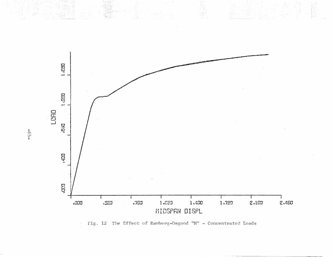
I01U1I

occo--l

8UJ

~l.:J

~to

~l---1

iI

8 'l

q -Y I ii' i I I.000 43Ea .700 l-sCED 1.400 1 .750 2.100 2.450

~.,:e; r ~{""'~R" f 0 I f""~Lj'IIuvl·· 'l~ vi

Fig. 12 The Effect of Ramberg-Osgood TTNTi

- Concentrated Loads

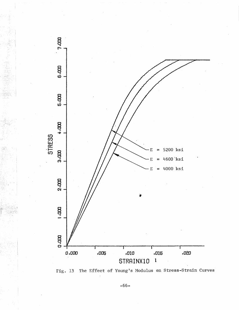
8o(0

8qO---t-----...,...-----...-------r------.------

~......

CJ)CJ)lLJ0::

-t-

~E = 5200 ksi

toE 4600 -'ksi(f) =E = 4000 ksi

8qC\I

'.8q

0.000 .oaa .010 .015

STRAINXIO 1

.oec

Fig. 13 The Effect of YoungTs Modulus on Stress-Strain Curves

-66-

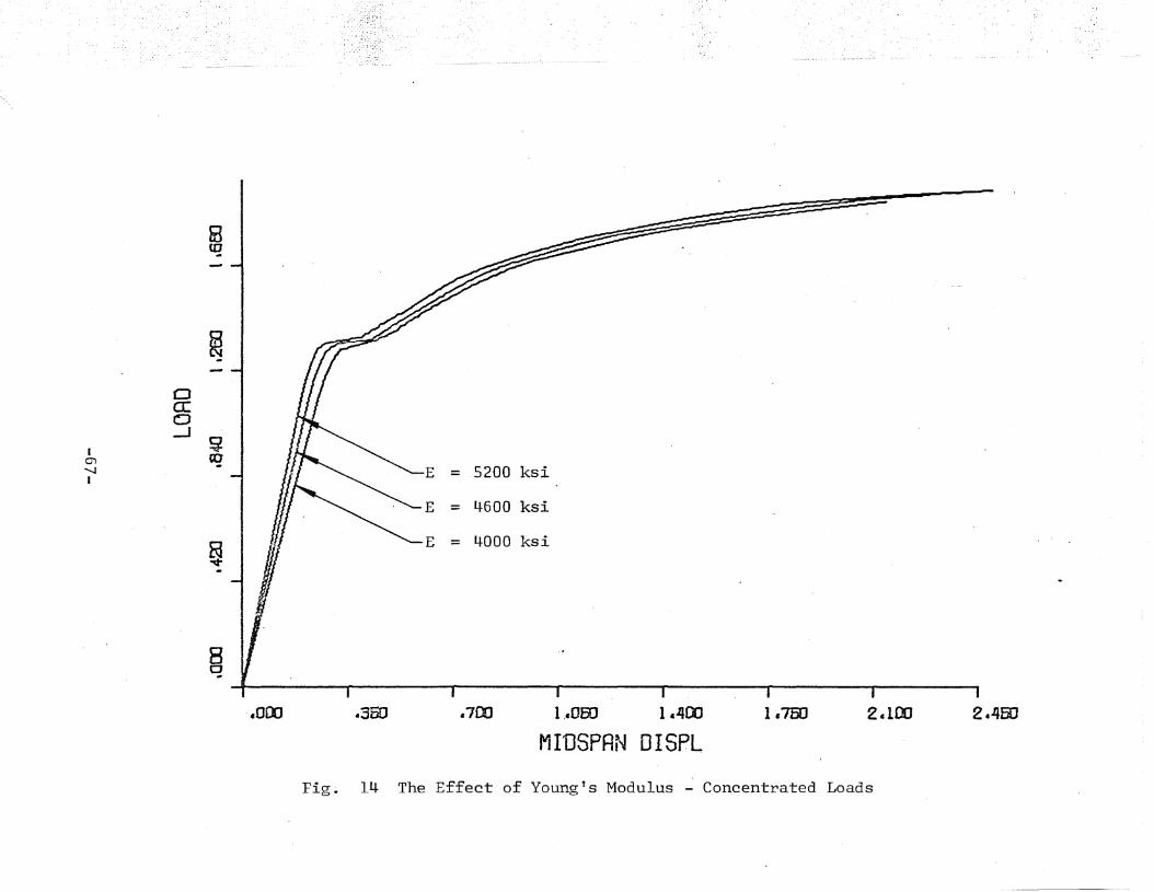
faID

~..."

0a:0.-J

~Ien «J'........ -I I/~~~E

= 5200 ksiI

E = 4600 ksi

@ I HI ~L = 4000 ksiv-

8q

·.000 .350 .700 1,.OEO 1.400 1.750 2.100 2.450

MIDSPRf\j 0ISPL

Fig. 14 The Effect of YoungTs Modulus - Concentrated Loads

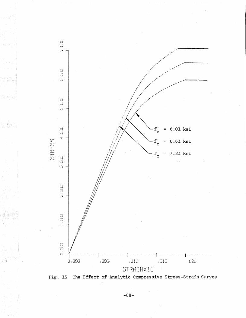
-,c015OcOOO

L7 --"---------

oLJCJ

\JJ

CJL)CJ

CJCJCJ

oL)C

C~

CJCjo

0 = 6.01 ksiC)0o.q.

([) fT = 6.61 ksi(f) cl.L_lCL: fT 7.21 ksiJ-- =(f) Lj C

L)<:"1(7'J

5TRRINXIOFig. 15 The Effect of Analytic Compressive Stress-Strain Curves

-68-

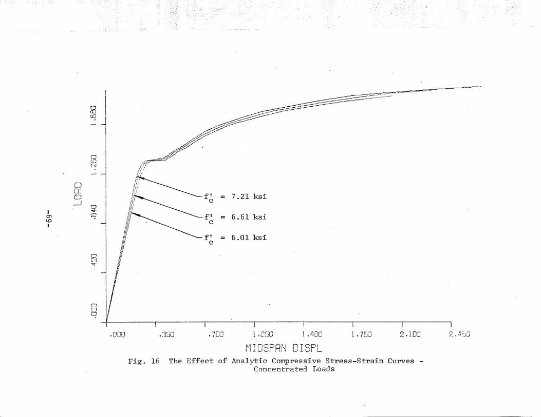
I I I I I l

.700 1 tOI50 1 «"'~OO 1 c7FjO 241.00 ~,j~)G

/~~~~-~-~

/-

.lElO

1{1

lilIff

~~ ~f~ = 7.21 ksiI()

d ~ft = 6.61 ksil~ c

$~ft = 6.01 ksiI c

f/

,.000

oCJo

oC·[~.

~ I~~

i

~'-... ~\,1

~JII

oITo.---.J

IenLCI

MI DSPRf~j 015PLFig. 16 The Effect of Analytic Compressive Stress-Strain Curves ­

Concentrated Loads

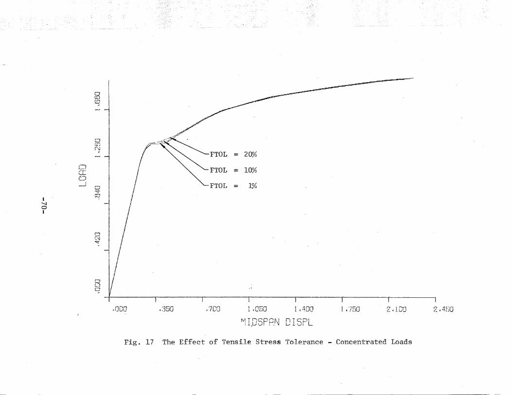
8ta~ I

--1II

0, ..-,u. ..f\l

FTOL = 20%

0I / ~~FTOL = 10%I

IT I0---J

0 I / "--FTOL = 1%-~

roI -'-JaI

0C\l-q--

oL.Jo

I I J I ---- ----------------l---------~ I

~OOO (:350 ~ 700 1c050 1 4 /~OO 1(750 2 c LCD 2 c "~EjO

f)1 I.05PPN 0I 5PL

Fig. 17 The Effect of Tensile Stress Tolerance - Concentrated Loads

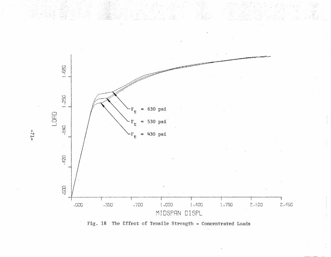
&3\S'

0:0(\J

: -l 1/~ ," " F

t= 630 psi

0 t 1 " "CL0

I I""

"-- F = 530 psiI t-----J

0-.c-

I

9?~ "'-F = -430 psi'-J I~ tI

o(\.1ooq'

aC~

o

~oco c3fjO ,700 1,050 1 t"~OO1 ' ..... 'C.r;I. ( ! .. )U 2.100 2 c llrJG

MI05PRf~ [J I 5PL

Fig. 18 The Effect of Tensile Strength - Concentrated Loads

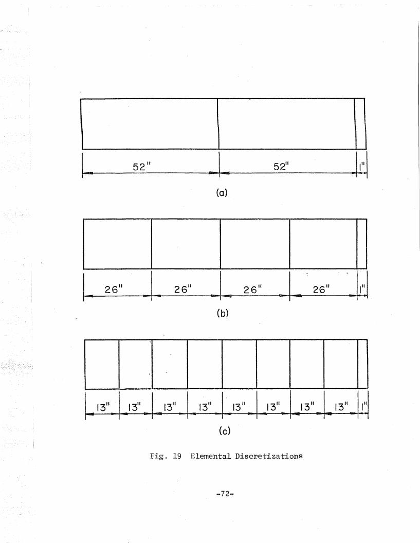
(0)

I~_26~"_~I_2 -----u611 _...............1__ 2-.-6II ~... 26"

(b)

I

1311 1311 1311

1311 13 II 13

11 1311

1311 III

- - - ::-- -- --

Fig. 19 Elemental Discretizations

-72-

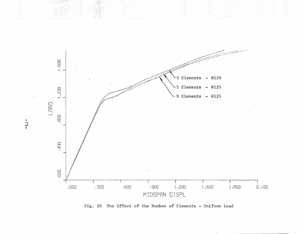
oL.J<.c

00r\J

--0

}IT

I0

I---J

0

IJC.)

I.CD

II'-JW

II

00'l'-

oLJo

'. ~ ~~;;;;;;;-::..:~:-:::.:---_.

~~:'~~:::~---------

~~/0'~_./J-./

_~.~<"/"'_ 3~/~_';-. ~. Elements - #124

_~ 5 Elements - #125

"- 9 Elements - #126

<000 .300 ~600 (r~DO 1 c200 1~SOOI I

1 (HOD 2.100

MfOSPRN DISPL

Fig. 20 The Effect of the Number of Elements - Uniform Load

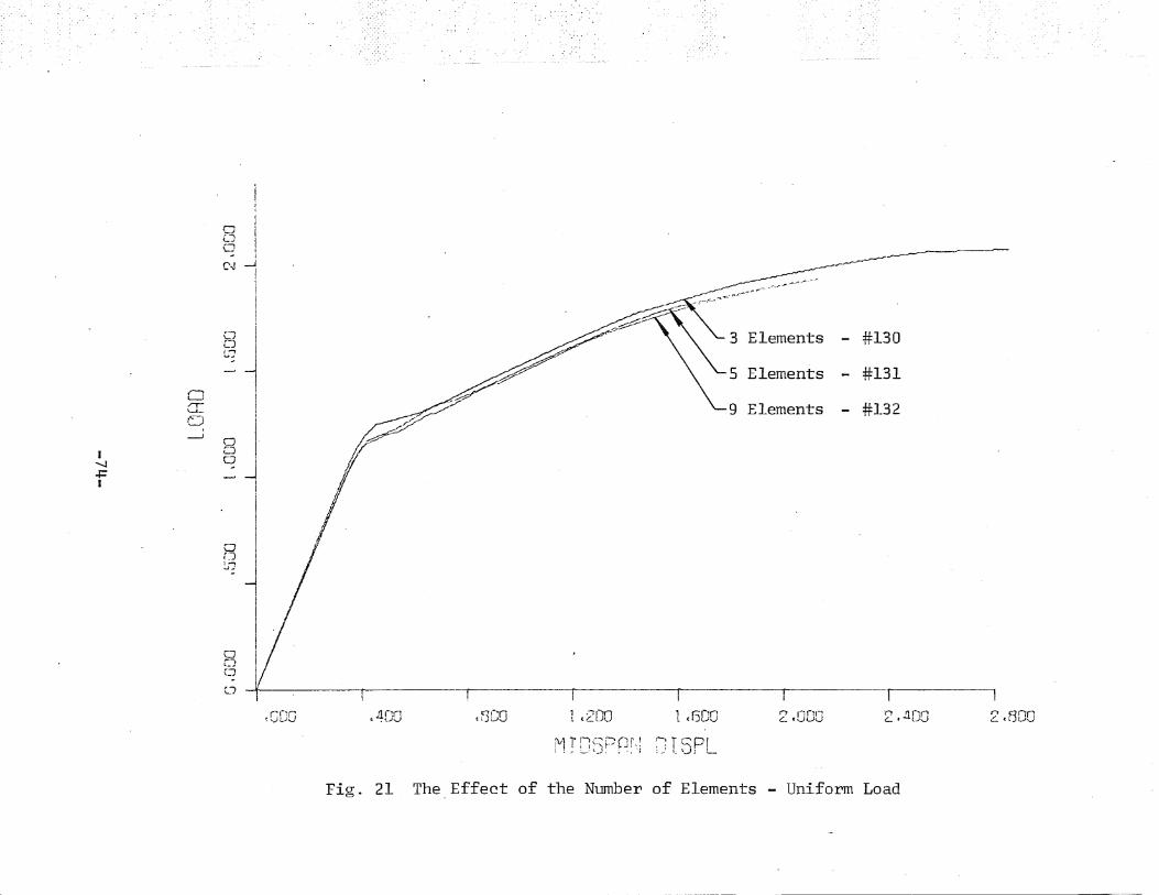
C)

oLJCJ

1 I

#131

- #130

.--------.

----------

9 Elements - #132

~

~

jII

IC'~ ~

!1j

~I

JI

oCJ~~

o;,L ....''I\.......

LjLJL-:'

---'

00=0

1--.J

I0

...........

0

-1=0

I

~GDO .ant!l: .(.';v tSCO 1 (2DO 1 (600 2,000 2.~DO 2c600

fVl r f-; ~~ p (] r-.~I •.'. :.....: _J. ;',' 015PL

Fig. 21 The Effect of the Number of Elements - Uniform Load

~ >

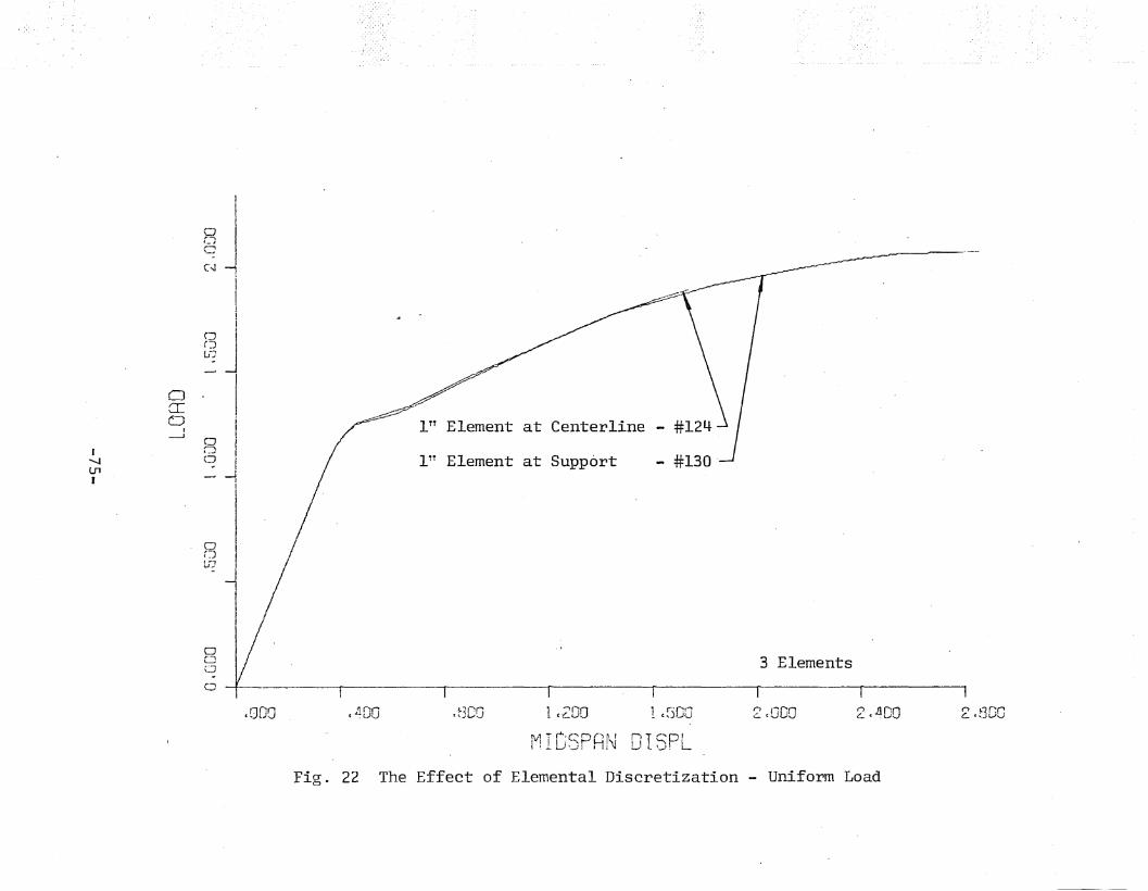
1

~JI_J

cC-J

It

I!I

i

OJ(:lUJ

0ICI

0 I r- ITT Element at CenterlineI I--J

0I 0

/ ITT Element at Support......... 0 IlJ1 __ -JI I

tI

or~1 -..,w ....

ooCJ 3 Elements

2 <t3GO2<400,000O-t- r I I I [ I I

(400 ~t3CO 1 (·200 1 (~50rJ 2<000

M;- C,c"'PR~ I n I r ... p'l!l ...J I i\l L..J.0. L

Fig. 22 The Effect of Elemental Discretization - Uniform Load

..----

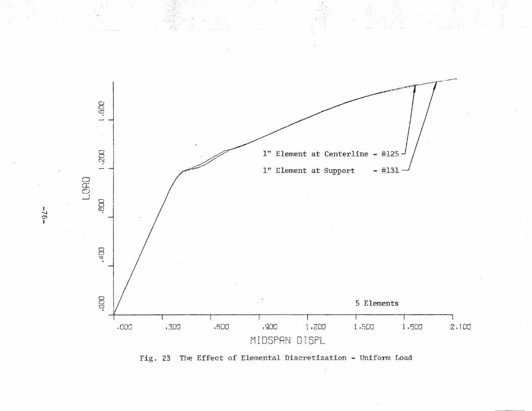
8\.C

0

I ;/ ITT Element at Centerline - #125cN

ITT Element at Support - #131I '"0

IT0

I---J

8I co

'..JC1J

oo~.

ooo 5 Elements

cODO (300 coOO ~900 1.200 1 ~500 1.800 2.100

MI 05PR~J 015PL

Fig. 23 -The Effect of Elemental Discretization - Uniform Load

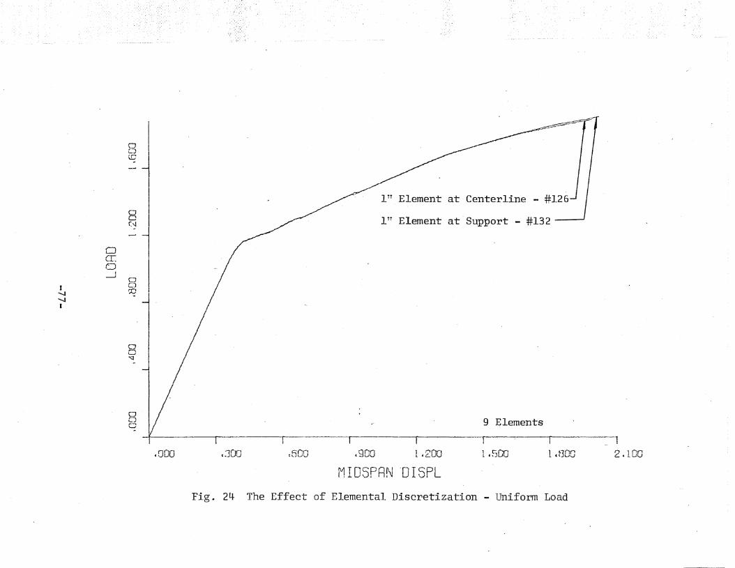
ITT Element at Centerline -

ITT Element at Support - #132

ao(C

00C'\l

----0IT0-'

I0

...........

Cl

........ro

I

oo~

oLJC 9 Elements

cODa cJOG :600 ,900 1,200 1.SOO 1 cr300 2 clOG

MID5PAN "DI5PL

Fig. 24 The Effect of Elemental Discretization - Uniform Load

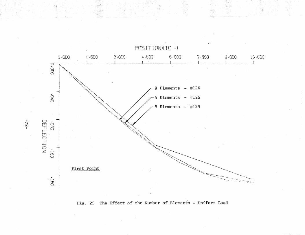
P0"0 I TIONX10 .- l

9,000 LG.500I I

7,500

#125

- '#124

- #126

6,D[JO

3 Elements

5 Elements

9 Elements

4.~OO3,0001,500

First Point

".'~"'~-It....

"\~

''''.,~,~~"'\"".

" '-

'.:"""'"'.~~ ",

..._~~"'~ ~

'.:'Z.....,~'......~.~

.,.~:~~~>"'-

'~~,"'-"'....~..,- "'

'~~';~""..,~~ ~~

'~~

..' ....~.~

.....~- ............

.....' ~

'~"..........:::.~

~~ '---,........~, ........-------

-~._.-- .---.,~.~----...::.::~:=.::~.::- '-- " :.c..~,>_

0.000

"'no

o Ii I ! I I I

aoLJ

~1o

I 0CJ'.J rr1 wOJ

--rt c."JIr-i-rln~l---t

0 ..z ....f')0

Fig. 2S The Effect of the Number of Elements - Uniform Load

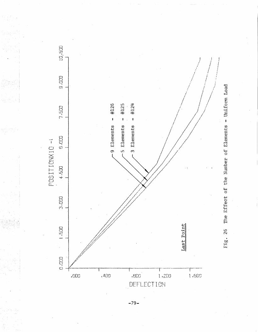
t.DN

1•fiDO1 t2[JQ

JlI/;

/ (

r i, .." I/

!

", ; iI

r } /l /I // /UJ L.l1 =t I/

N N N i / Ir-I r-I r-I /' f /* :tt: :tt: I

I / /"I .1/

I /en en rn

;/.J-J .J-J .J-JJ=: ~ J=: /Q) OJ OJE S S J

)

QJ OJ OJ ) /1r-I r-I r-I

/r..L1 r.J..1 r.J..1

m L.n M I)'

/~

I,4DO.000

ooLlJ

CJo';-1WoO

o'..... ..J

oou~

CJC)o

oCJo<.rJ-

--J----I

xzo~

Ir--~l

(f)o(L

o

DE·<F--f [L~T I (1 hI.- 1_••. , WI

-79-

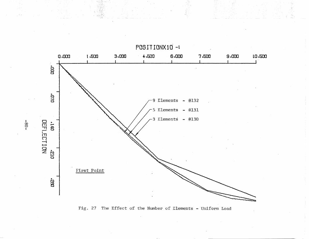
POSITIONX10 -1

0.000 1,500 3,000 < +.600 6,000 7.500 9.000 LO .500

..a8

.0

c3 I ~, ;-9 Elements - #132

5 Elements - #131

I 0 ---. '- '- / / / 3 Elements - #13000

a

a rrI ,..-.I "b,

rnn-1.......Q

III:z: f':)j.o..I

c

First Point

.t")

B

Fig. 27 The Effect of the Number of Elements - Uniform Load

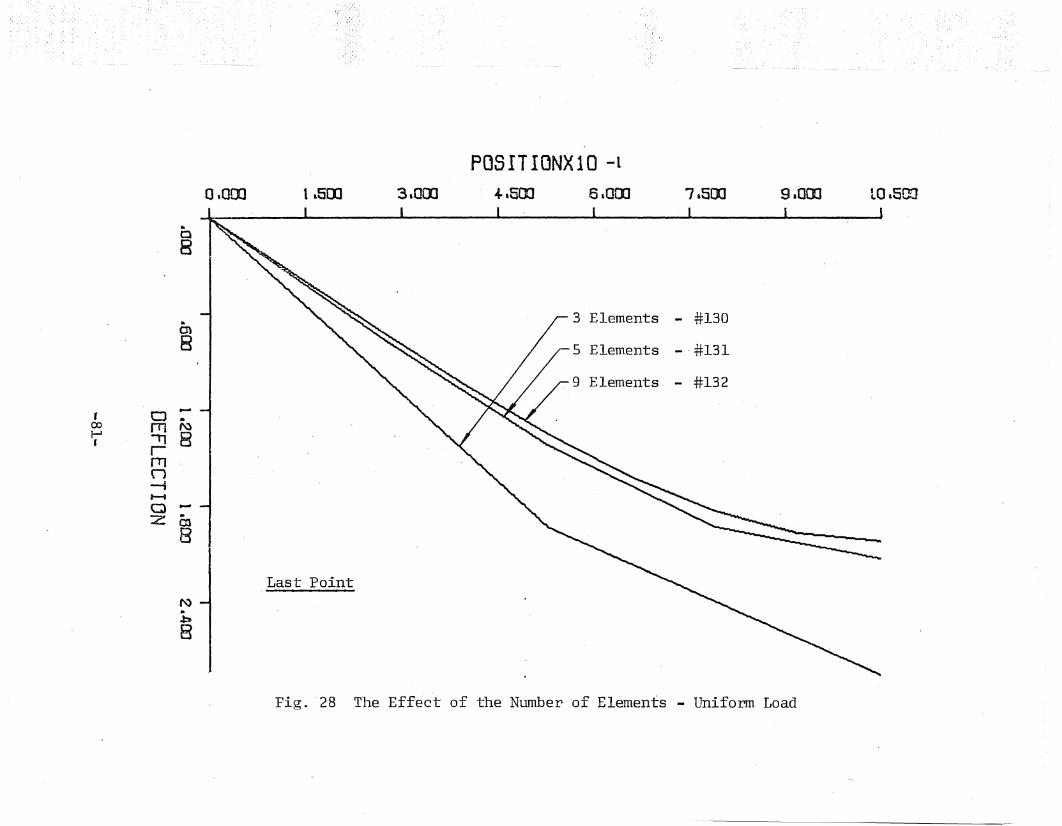
POSITIONX10 --l

0,000 1 .500 3.000 ~,5OJ 6,000 7.500 9.000 to.EOO

..c8

. I

en, ...............

8 I

/ 3 Elements - #130

'" '-"- / - 5 Elements - . #131

, 0:-- I ,~//

Elements

co

- #132

f-'rnl\.)

I .." 8rrnn--tt--IQ .....:z en

8

Last Pointf\).~

8

Fig. ·28 The Effect of the Number of Elements - Uniform Load

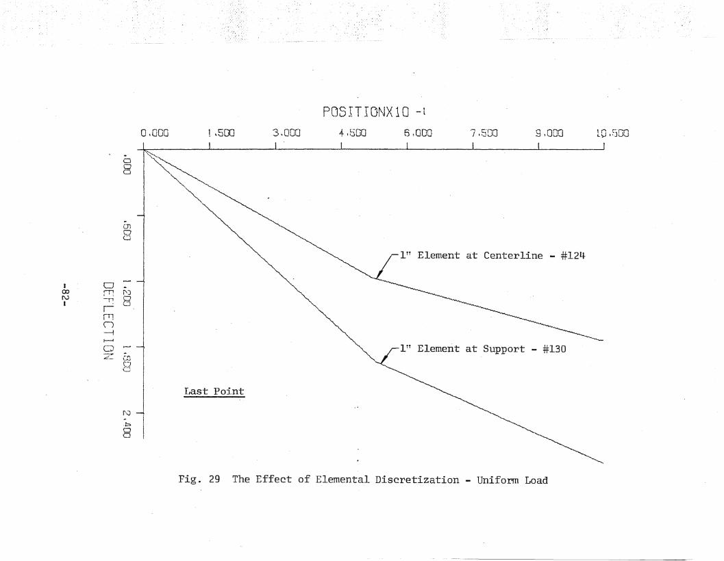
POSIT I uNX10 - 1

0\000

§ I'~

J-01oo

1~500 3~OOO 4-,500 6~OOO 7~500 9,000 LOl500

I 000N

illI 11

riTln-It--f

0Z

1')oo

wC~)

C

r·~ J.~~ i8 I

Last Point

ITT Element at Centerline - #124

ITT Element at Support - #130

Fig. 29 The Effect of Elemental Discretization - Uniform Load

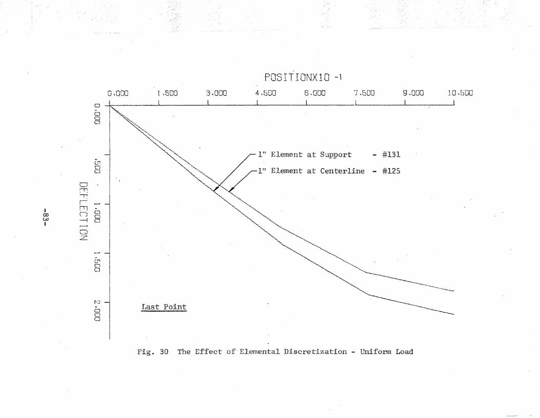
P05ITIONX10 -1

1TT Element at Centerline

#131

- #125

7 \500 9 .000 10 ~fjGO

1 1 1

ITT Element at Support

o,oeo 1 \500 3,000 4.500 6\000

§t~ l I I I

~~

~"""- ~,~

c.J!CJ0

CJ;r:----ro1rrl ...

I(J c....J

CXJ 0UJ ----1 c..~I r---t

0z·

1-

-c..~C/0

---..._- .._-..._--r<J-aCJo

Last Point

Fig. 30 The Effect of-Elemental Discretization - Uniform Load

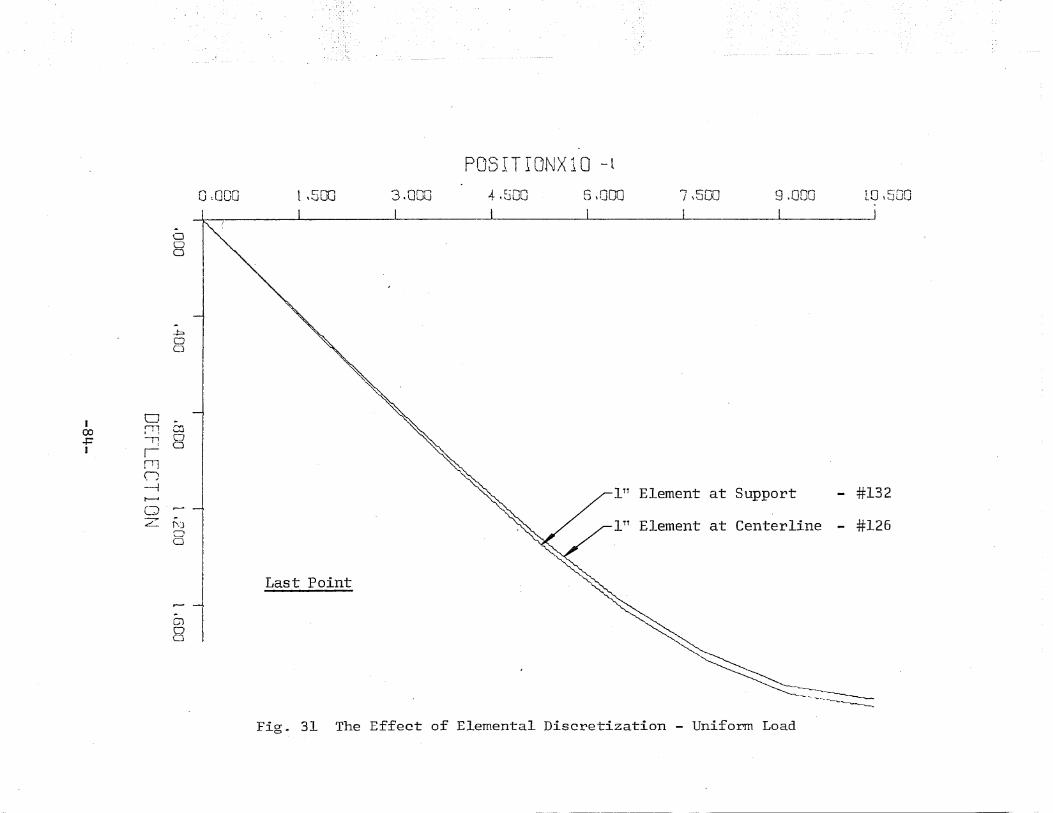
P03 ITION X10 - t

o~ooo 1\500 3.000 4- tEjOO 6,000 7 \500 9.000 1.0\500

...aoo

111 Element at Centerline - #126

,~~=~-~

- #132ITT Element at Support

Last Point

.....poo

enoa

f\)oo

I

I

§l

I 0co :rl+=' '1I I

rr1n---J~

(-;:Jz

Fig. 31 The Effect of Elemental Discretization - Uniform Load

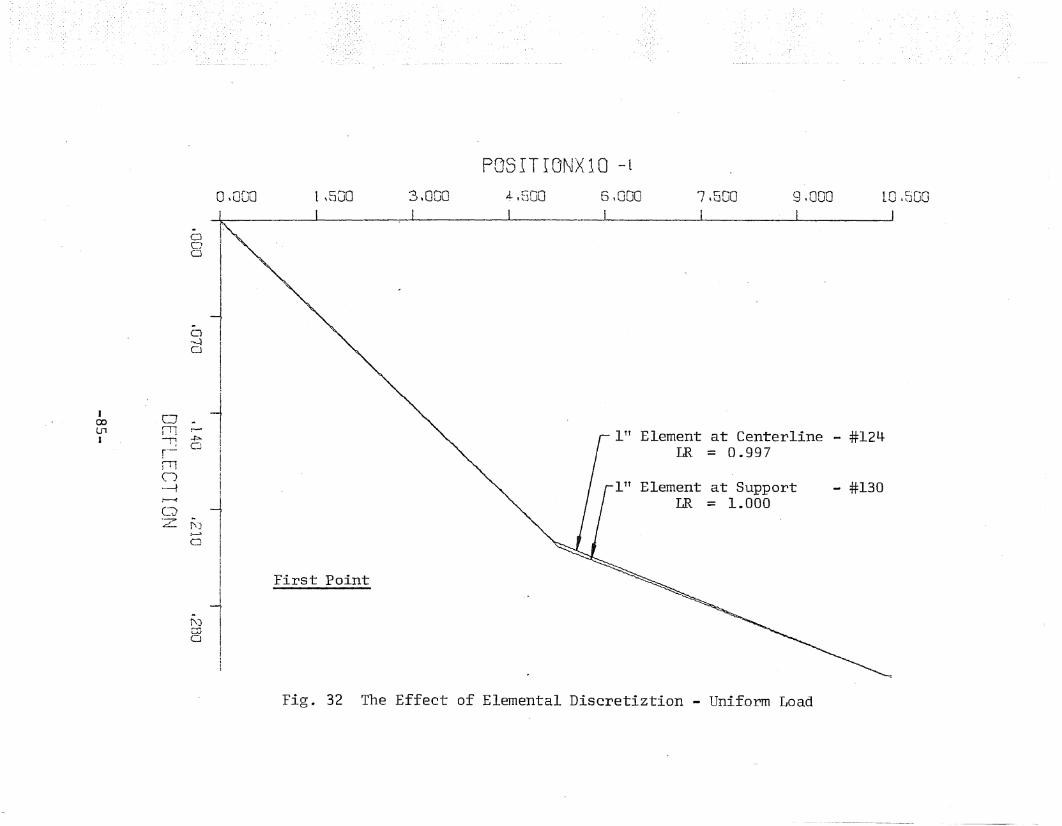
P05ITIONX10 -1

0,000

..oC)o

t \500 3,000 4- ,~JOO 6,000 7,500 9,000 LO ,fjGO

Element at Centerline - #124LR = 0.997

I 000Ln nlI ;;

r--J1ln.~

:----t

C-:J·z

o

cJ II

:-1~~ Io i

II

Jj":J~

o

I

~II!I

First Point

Element at SupportLR = 1.000

- #130

Fig. 32 The Effect of Elemental Discretiztion - Uniform Load

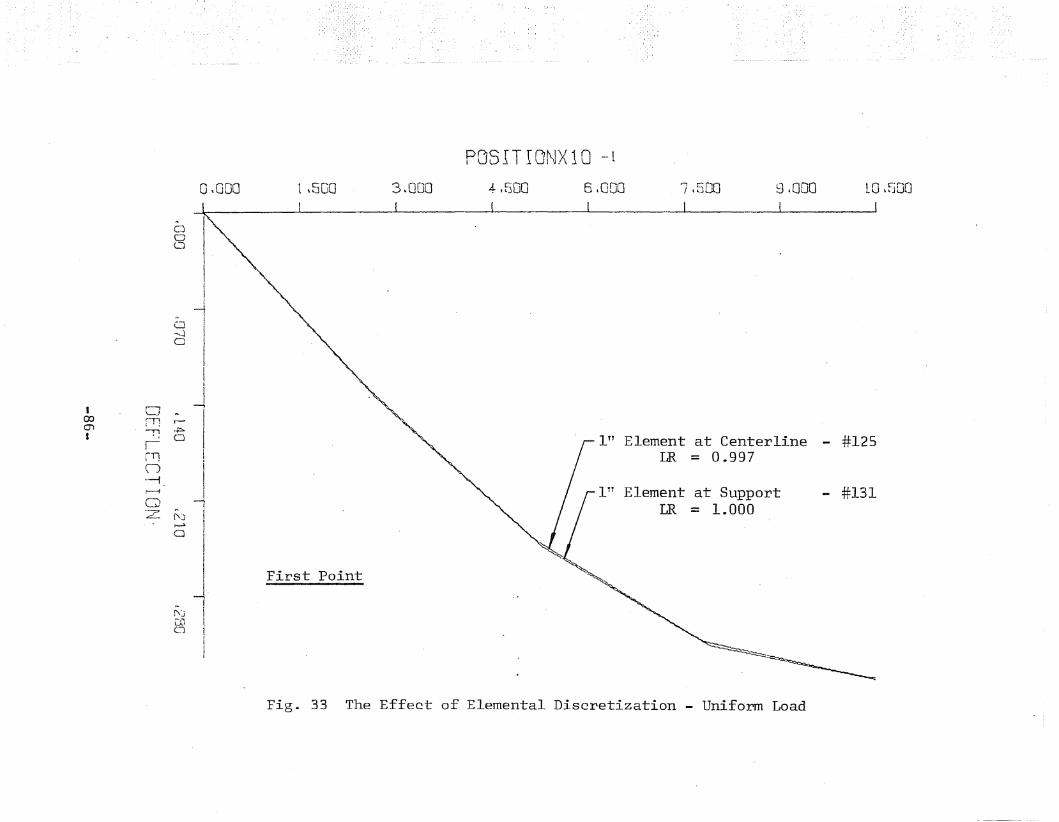
PDS ITI ONX 10 - t

0,000 1,5DO 3,000 41500 6,000 7 l5DO g~OOO LO \fjOO

ooo

..o-.:Io

II

---l11

II

I 0J

00.... Im ill r-

I ~...p....0

t

I Iill I

I

n i--1 I:----f

i

QI

.~

4~ f\.) I~

a

I~

~" I' JCD I(,--:1 j

1IIII

First Point

Element at Centerline - #125LR = 0.997

Element at Support - #131LR = 1.000

~Fig. 33 The Effect of Elemental Discretization - Uniform Load

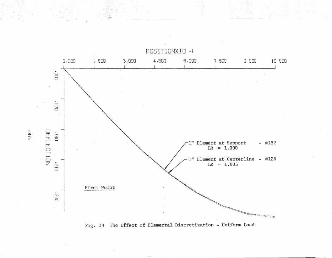
POS IT IONX 10 -l

o~ooo

.§\

I

S~a I

~ III

1,500 3,000 41500 6\000 7 l500 9.000 10.FjGO

~~--=--:o.o,,---;::_-::, :::=:

1 11 Element at Centerline - #126LR = 1.005

Ico

0......... ;T1

I -r:!fIln-tt--{

0Z

,-...po.a

~ I

Jf\J jCD !o !

I

First Point

111 Element at SupportLR = 1.000

- #132

Fig. 34 The Effect of Elemental Discretization - Uniform Load

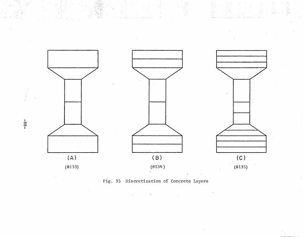
I00COI

(A)

(#133)

( B)

(#134 )

(C )

(#135)

Fig. 35 Discretization of Concrete Layers

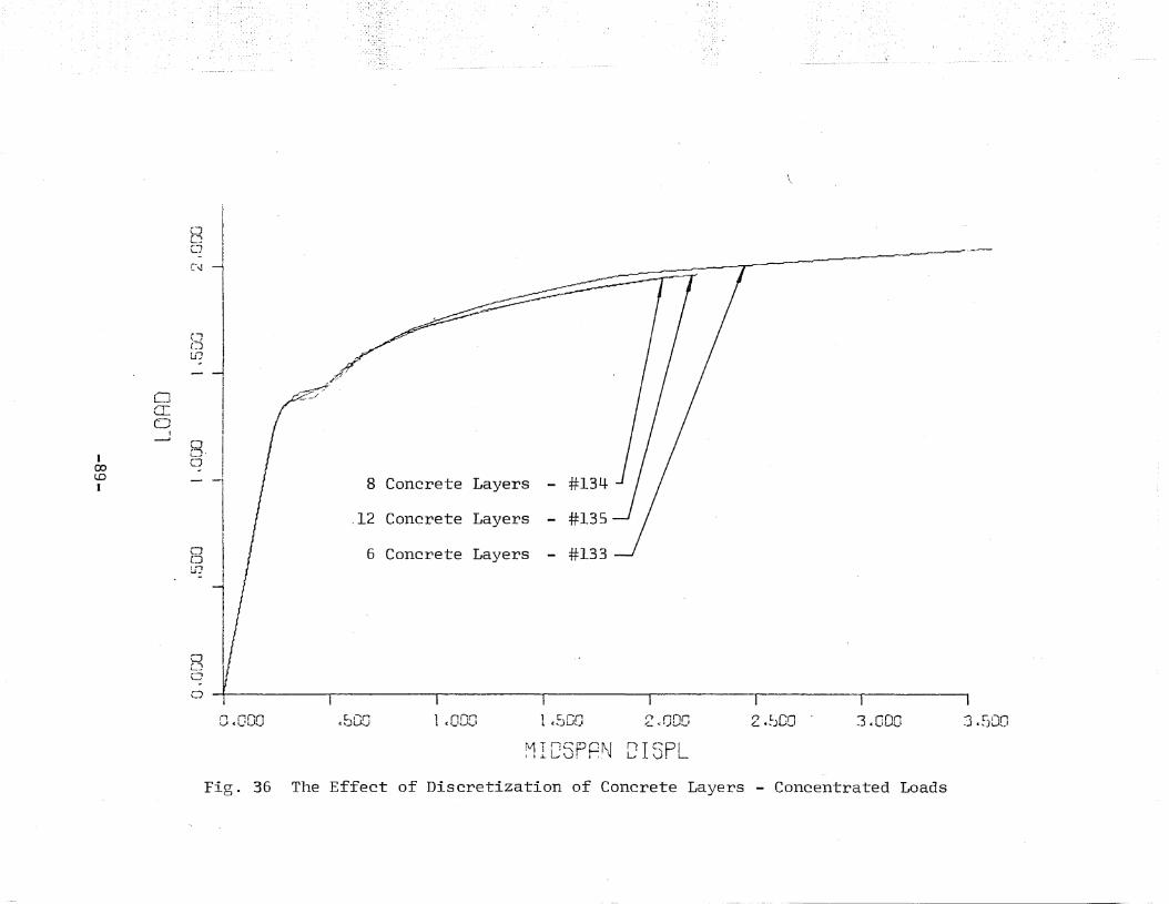
o'"""L_

a

\

Ic;L-:1Lj-

C.J

I~

I ~C;(~

1..iJ I

/I ..//

0 IITI0

f I~

8·I

I LJ00 ...lD -I 1 8 Concrete LayersI

I I .12 Concrete Layers

0I

I 6 Concrete LayersCJLJ'"] I

2 .~JOO .2~ODO1 4;JCQ1 <000cSGO0.000

o ~ I i j i I I I

3.000 3.500

MTr:~PQN n Ic~PLI i.l..L...oV. J._ L.V

Fig. 36 The Effect of Discretization of Concrete Layers - Concentrated Loads

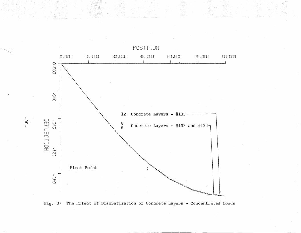
P j>;~ TT rON,.....1L/~. , _

4~ ,G[jO30 lOfJOl5.DeJO[JI(]DO 60.000 75,000 90,000o -l I I I I I I l

12 Concrete Layers - #135 I

86 Concrete Layers - #133 and #134

,-- 'II.. ~..;

a

I~ ...~

~--.~~~

~.~

-"':~,,:: ..,......

Fig. 37 The Effect of Discretization of Concrete Layers - Concentrated Loads

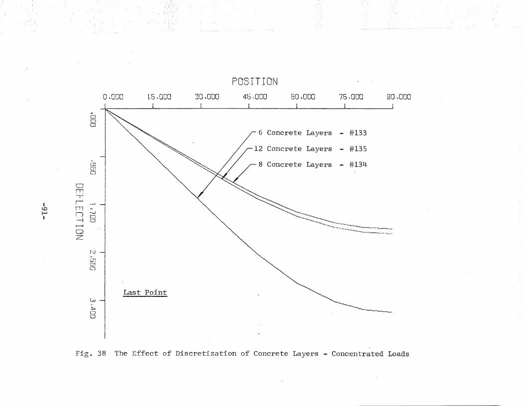
POSITION0,000 lS~OOO 30,000· 4~) ~OOO 60,000 75tOOO 90,000

IlDf-JI

...aoa

..C1j[51o

ofT1--;t

r­rn ...n (3-4 CJ~

C)Z

r~J

-Gr"}[,'1LJ

w,~

oo

Last Point

6 Concrete Layers - #133

12 Concrete Layers - #135

8 Concrete Layers - #134

""-----~ --~_._----------~-~-~--

Fig. 38 The Effect of Discretization of Concrete Layers - Concentrated Loads

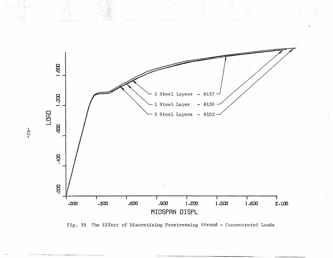
8~

Bo· J i':'

BU?

§ I "...-- " "-... - 2 Steel Layers - #137

-

I /' 1 Steel Layer - #136

CJ ~ 3 Steel Layersa: - #102C)--I

§ILONI

.000 .-300 .600 .900 1.200 1.500 1.600 2.100

MIDSPAN DISPL

Fig. 39 The Effect of Discretising -Prestressing Strand - Concentrated Loads

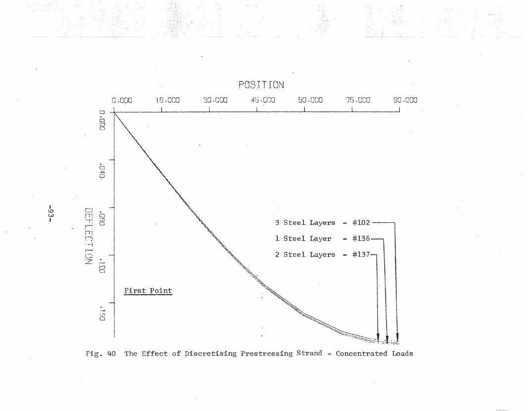
PDS I TIOf\J

o ,OeJO 15,O[JO 30tCOO 4~j ,GDO SOIODO 'Ie r"r"'nI") 'U~)I...,..; 90,[][JO

oooC~

...o~o

ICJr..o ..

lJJ f1: LJI --rJ ~~

!0

ill\J"--1r--i

0Z

..r....-,C}

~j)

o

First Point

3 Steel Layers - #102 i

1 Steel L?ye.r - #136

" 2 Steel Layers - #137~-

""-,,~~~,

~-.:',,~

~~

~~~

--...::..~--~

--~.:;..~~:~-::~ .,-~ ....--Fig. 40 The Effect of Discretising Prestressing Strand - Concentrated Loads

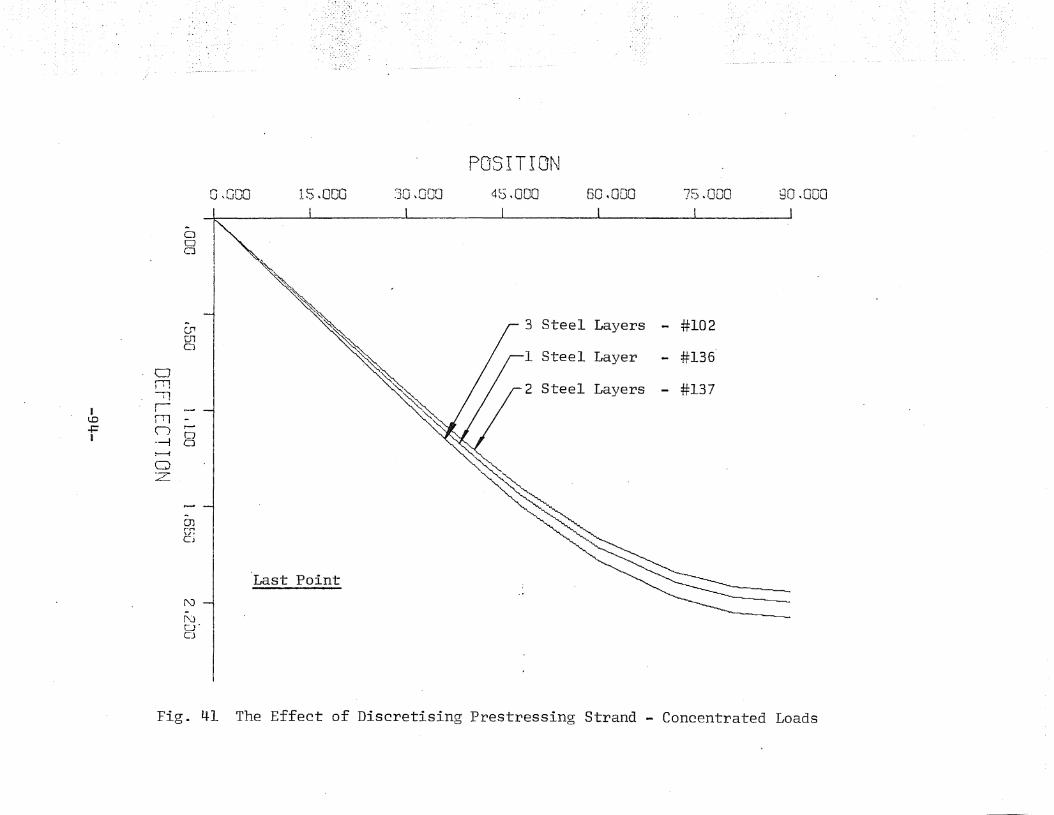
o,~GOO 15~OOO :30,000

POSITION4~) .000 60.000 7S~OOO 90,000

Il.D+:I

G"Dlo

CJill-nr­t

rTl:(J 0.---1 0~

C)

z

OJr-ncj

N

NU"CJ

Last Point

3 Steel Layers

1 Steel Layer

2 Steel Layers

- #102

- #136

- #137

Fig. 41 The Effect of Discretising Prestressing Strand - Concentrated Loads

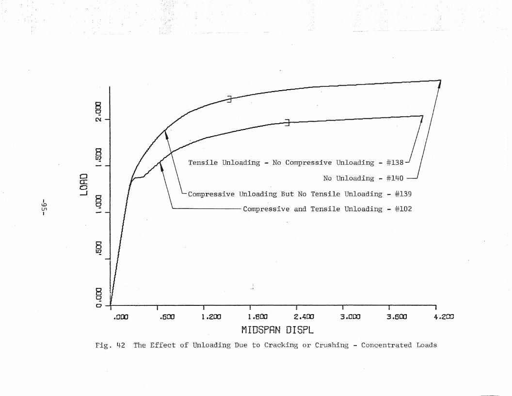
No Unloading - #140

Tensile Unloading - No Compressive Unloading - #138

Compressive Unloading But No Tensile Unloading - #139

, Compressive and Tensile Unloading - #102

Bqo , iii'"

8U7

N

§

8Lq-

Cla:c::J--l

J 8t..DlJl

qI

.000 .600 1.200 1.600 2.400 3.000 3.600 4.200

MIDSPAN DISPLFig. 42 The Effect of Unloading Due to Cracking or Crushing - Concentrated Loads

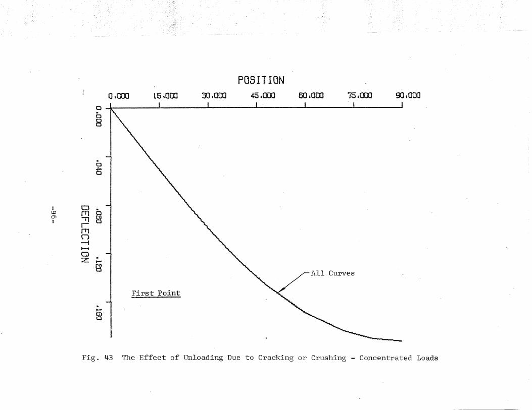
0.000 L5.000 30.000

POSITION45.000 60.000 75.000 90,000

All Curves

First Point

.o~

o -l I , , ' J !..a8

.to-

El

CJ •fT1 0

" BrJI1.n--It-t

Q.Z ,...

e1

ILDenI

Fig. 43 The Effect of Unloading Due to Cracking or Crushing - Concentrated Loads

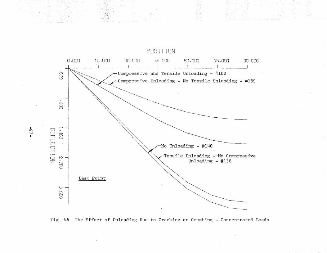
POSITION0,000 L5.000 30,iJOO 4~J ,000 50,000 7~) tODD 90,000

Cl......-)

Q

10

tooo

Compressive and Tensile Unloading - #102

~CompressiveUnloading - No Tensile Unloading - #139

~

~~~ ..

. ~-----I

~_Jl.D'-J f"l; 'J-J

I ~ C'JI! CJr

iil.n~~

(:J r\)

Z........,JrI

(~

I

I . Last PointI

~j --t~;

IC"7CJ

i

No Unloading - #140

Tensile Unloading --No CompressiveUnloading - #138

'~

~-----------Fig. 44 The Effect of Unloading Due to Cracking or Crushing - Concentrated Loads

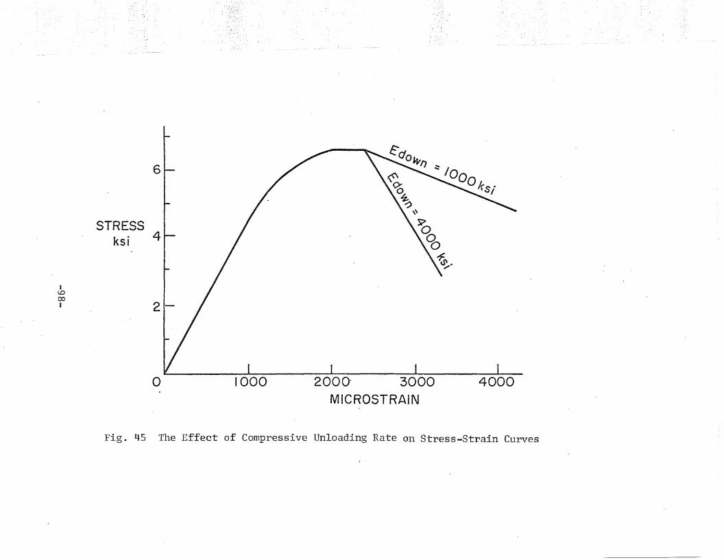
40-00

~/OO

°lrsi

2000' 3000MICROSTRAIN

1000

2

6

4

o

STRESSksi

JtD00I

Fig. ~5 The Effect of Compressive Unloading Rate on Stress-Strain Curves

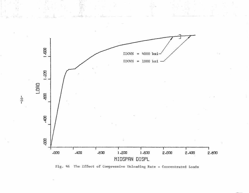
-I ~--------- ----,--- I I -.

1.200 1.500 2 .000 2.400 2 .800

f1 IDSPAN 0ISPL.500.400.000

~

§

~ I ~ EDOWN = 4-000 'ksi

EDOWN = 1000 ksi, J

~-CJa:LJ--1

§ILDlDI

Fig. 46 -The Effect of Compressive Unloading Rate - Concentrated Loads

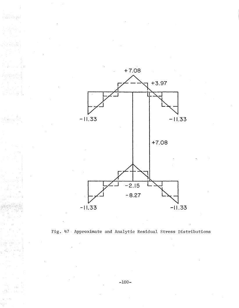
+3.97

+7.08

-11.33 -11.33

+7.08

-11.33

-2.15

-8.27

-11.33

Fig. 47· Approximate and Analytic Residual Stress Distributions

-100-

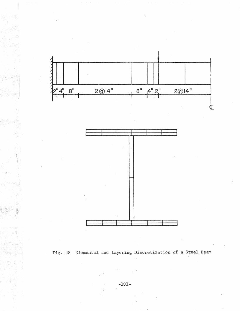
8 11 4 11 2 11 2@14 11I

~.. +-t1---mq--=--------1~

I.I

/.I//;"

//A--""""-......a-----a...-------------I ....I---L-l.. ...L- --I/

/2"411;' I I

t I

II

II

II

II

II

II

1I

.-

rr

II

II

-,I

,I

II

II

Fig. 48 Elemental and Layering Discretization of a Steel Beam

-101-

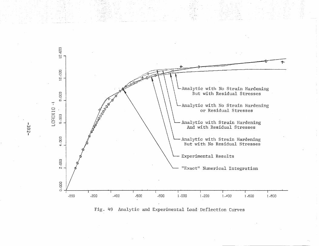
Bo(..J-..I

1TExactTT Numerical Integration

Experimental Results

Analytic with No Strain Hardeningor Residual Stresses

Analytic with Strain HardeningAnd with Residual Stresses

. Analytic with Strain HardeningBut with No Residual Stresses

\-~AnalYtic with No Strain HardeningBut with Residual Stresses

8o(\oj

oot.J

o

00C!

- (Co

,0~

X0

00

IIT 0

f-J

0 to

0-.J

NI

0aC?'"d-

oooo

.000 .200 .400 .500 .600 1.000 1.200 llA OO 11600 1.SCO

Fig. 49 Analytic and Experimental Load"Deflection Curves

6 • REFERENCES

1. FORTRAN REFERENCE MANUAL, REVISION E, Control DataCorporation, Sunnyvale, California, 1971.

2. FORTRAN EXTENDED REFERENCE MANUAL, REVISION H, ControlData Corporation, Sunnyvale, California, 1971.

3. SCOPE 3.3 REFERENCE MANUAL, REVISION C, Control DataCorporation, Sunnyvale, California, 1971.

4. Galambos, T. V.STRUCTURAL MEMBERS AND FRAMES, 'Prentice-Hall, 1968.

s. Hanson, J. M. and Hulsbos, C. L.OVERLOAD BEHAVIOR OF PRESTRESSED CONCRETE BEAMS WITHWEB REINFORCEMENT, Fritz Engineering Laboratory ReportNo. 223.25, February 1963.

6. Hanson, J. M. and Hulsbos, C. L.ULTIMATE SHEAR STRENGTH OF PRESTRESSED CONCRETE BEAMSWITH WEB REINFORCEMENT, Fritz Engineering LaboratoryReport No. 223.27, April 1965.

7. Knudsen, K. E., Yang, C. H., Johnston, B. G. and Beedle, L. S.PLASTIC STRENGTH AND DEFLECTIONS OF CONTINUOUS BEAMS,The Welding Journal Research Supplement, May 1953.

8. Kulicki, J. M. and Kostem, C. N.THE INELASTIC ANALYSIS OF REINFORCED AND PRESTRESSEDCONCRETE BEAMS, Fritz Engineering Laboratory ReportNo. 378B.l, November 1972.

9. Kulicki, J. M. and Kostem, C. N.A USER'S MANUAL FOR PROGRAM BEAM, Fritz EngineeringLaboratory Report No. 378B.2, February 1973.

-103-

10. Kulicki, J. M. and Kostem, C. N.APPLICATIONS OF THE FINITE ELEMENT METHOD TO INELASTICBEAM COLUMN PROBLEMS, Fritz Engineering LaboratoryReport No. 400.11, March 1973.

11. Zienkiewicz, o. C.THE FINITE ELEMENT METHOD IN ENGINEERING SCIENCE,McGraw-Hill, London, England, 1971.

-104-

7 • ACKNOWLEDGMENTS

This study was conducted in the Department of Civil

Engineering at the Fritz Laboratory, Lehigh University, Bethlehem,

Pennsylvania.

The authors wish to extend their thanks to the staff of

the Lehigh University Computing Center for their cooperation.

Thanks is also extended to Mrs. Ruth Grimes who typed the manu­

script and to Mr. John Gera and Mrs. Sharon Balogh who traced some

of the figures.

-105-